Bit Error Rate Analysis
Analyze BER performance of communications systems
Description
The Bit Error Rate Analysis app calculates the bit error rate (BER)
as a function of the energy per bit to noise power spectral density ratio
(Eb/N0).
Using this app, you can:
-
Generate BER data for a communications system and analyze performance using:
-
Monte Carlo simulations of MATLAB® functions and Simulink® models.
-
Theoretical closed-form expressions for selected types of
communications systems. -
Run systems contained in MATLAB simulation functions or Simulink models. After you create a function or model that
simulates the system, the Bit Error Rate Analysis app
iterates over your choice of
Eb/N0
values and collects the results.
-
-
Plot one or more BER data sets on a single set of axes. You can graphically
compare simulation data with theoretical results or simulation data from a
series of communications system models. -
Fit a curve to a set of simulation data.
-
Plot confidence levels of simulation data.
-
Send BER data to the MATLAB workspace or to a file for further processing.
For more information, see Analyze Performance with Bit Error Rate Analysis App.

Open the Bit Error Rate Analysis App
-
MATLAB Toolstrip: On the Apps tab, under
Signal Processing and Communications, click the app
icon. -
MATLAB command prompt: Enter
bertool.
Examples
expand all
Compute BER Using Theoretical Tab
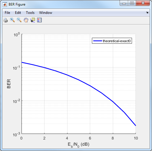
Generate a theoretical estimate of BER performance for a
16-QAM link in AWGN.
Open the Bit Error Rate Analysis app.
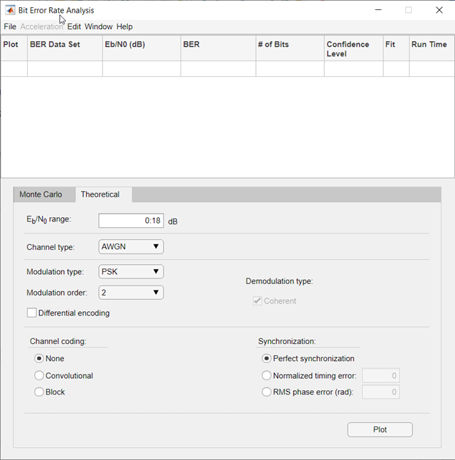
On the Theoretical tab, set these parameters to the specified values:
Eb/N0
range to 0:10, Modulation
type to QAM, and Modulation
order to 16.
Plot the BER curve by clicking Plot.
Compute BER Using Monte Carlo Tab and MATLAB Function Simulation
Simulate the BER by using a custom MATLAB function. By default, the app uses the
viterbisim.m simulation.
Open the Bit Error Rate Analysis app.
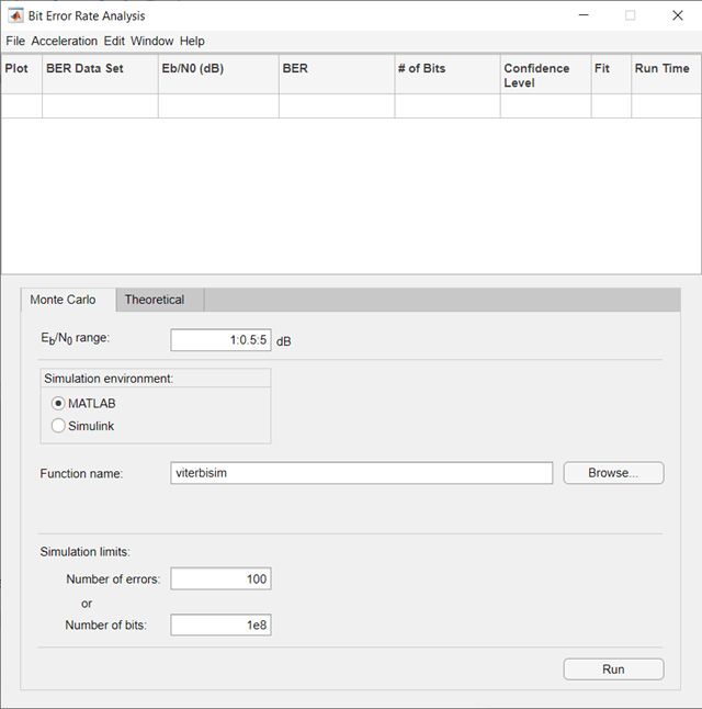
On the Monte Carlo tab, set the Eb/N0
range parameter to 1:.5:6. Run the
simulation and plot the estimated BER values by clicking
Run.
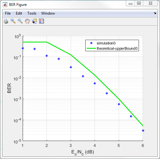
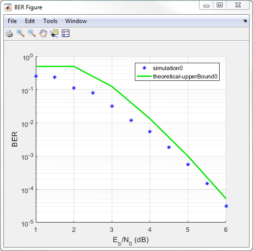
On the Theoretical tab, set Eb/N0
range to 1:6 and set Modulation
order to 4. Enable convolutional
coding by selecting Convolutional. Click
Plot to add the theoretical upper bound of the BER
curve to the plot.
Prepare MATLAB Function for Use in Bit Error Rate Analysis App
Add code to the simulation function template given in the
Template for Simulation Function topic to run in the Monte
Carlo tab of the Bit Error Rate Analysis.
Prepare Function
Copy the template from the Template for Simulation Function topic into a new MATLAB file in the MATLAB Editor. Save the file in a folder on your MATLAB path, using the file name
bertool_simfcn.
Place lines of code that initialize parameters or create objects used in
the simulation in the template section marked Set up initial. This code maps simulation variables to the
parameters
template input arguments. For example, snr maps to
EbNo.
% Set up initial parameters.
siglen = 1000; % Number of bits in each trial
M = 2;         % DBPSK is binary
snr = EbNo;    % Because of binary modulation

% Create an ErrorRate calculator System object to compare
% decoded symbols to the original transmitted symbols.
errorCalc = comm.ErrorRate;
Place the code for the core simulation tasks in the template section
marked Proceed with simulation. This code includes the
core simulation tasks, after all setup work has been performed.
    msg = randi([0,M-1],siglen,1); % Generate message sequence
    txsig = dpskmod(msg,M);        % Modulate
    hChan.SignalPower = ...        % Calculate and assign signal power
        (txsig'*txsig)/length(txsig);
    rxsig = awgn(txsig,snr,'measured'); % Add noise
    decodmsg = dpskdemod(rxsig,M);      % Demodulate
    berVec = errorCalc(msg,decodmsg);   % Calculate BER
    totErr = totErr + berVec(2);
    numBits = numBits + berVec(3);
After you insert these two code sections into the template, the
bertool_simfcn function is compatible with the
Bit Error Rate Analysis app. The resulting code resembles
this code segment.
function [ber,numBits] = bertool_simfcn(EbNo,maxNumErrs,maxNumBits,varargin)
%
%   See also BERTOOL and VITERBISIM.

% Copyright 2020 The MathWorks, Inc.

% Initialize variables related to exit criteria.
totErr = 0;  % Number of errors observed
numBits = 0; % Number of bits processed

% --- Set up the simulation parameters. ---
% --- INSERT YOUR CODE HERE.
% Set up initial parameters.
siglen = 1000; % Number of bits in each trial
M = 2;         % DBPSK is binary.
snr = EbNo;    % Because of binary modulation
% Create an ErrorRate calculator System object to compare
% decoded symbols to the original transmitted symbols.
errorCalc = comm.ErrorRate;

% Simulate until the number of errors exceeds maxNumErrs
% or the number of bits processed exceeds maxNumBits.
while((totErr < maxNumErrs) && (numBits < maxNumBits))

    % Check if the user clicked the Stop button of BERTool.
    if isBERToolSimulationStopped(varargin{:})
      break
    end

    % --- Proceed with the simulation.
    % --- Update totErr and numBits.
    % --- INSERT YOUR CODE HERE.
    msg = randi([0,M-1],siglen,1); % Generate message sequence
    txsig = dpskmod(msg,M);        % Modulate
    hChan.SignalPower = ...        % Calculate and assign signal power
        (txsig'*txsig)/length(txsig);
    rxsig = awgn(txsig,snr,'measured'); % Add noise
    decodmsg = dpskdemod(rxsig,M);      % Demodulate
    berVec = errorCalc(msg,decodmsg);   % Calculate BER
    totErr = totErr + berVec(2);
    numBits = numBits + berVec(3);
end % End of loop

% Compute the BER.
ber = totErr/numBits;
The function has inputs to specify the app and scalar quantities for
EbNo, maxNumErrs, and
maxNumBits that are provided by the app. The Bit
Error Rate Analysis app is an input because the function monitors
and responds to the stop command in the app. The
bertool_simfcn function excludes code related to
plotting, curve fitting, and confidence intervals because the Bit Error
Rate Analysis app enables you to do similar tasks interactively
without writing code.
Use Prepared Function
Run bertool_simfcn in the Bit Error Rate
Analysis app.
Open the Bit Error Rate Analysis app, and then select the
Monte Carlo tab.
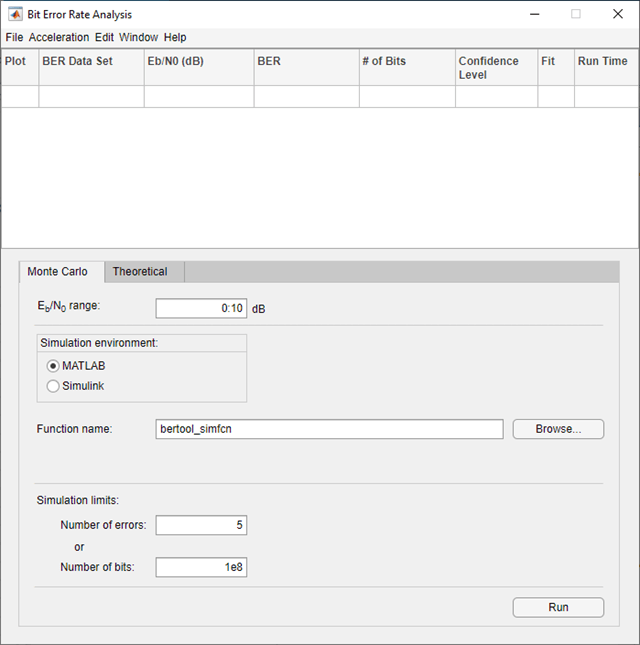
Set these parameters to the specified values:
Eb/N0
range to 0:10, Simulation
environment to MATLAB, Function
name to bertool_simfcn, Number
of errors to 5, and Number of
bits to 1e8.

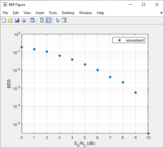
Click Run.
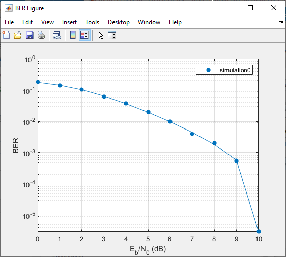
The Bit Error Rate Analysis app computes the results and then
plots them. In this case, the results do not appear to fall along a smooth
curve because the simulation required only five errors for each value in
EbNo.
Fit a curve to the series of points in the BER Figure window, by selecting
the Fit parameter in the data viewer.

The Bit Error Rate Analysis app plots the fitted curve, as
shown in this figure.
Compute Error Rate Simulation Sweeps Using Bit Error Rate Analysis App
Use the Bit Error Rate Analysis app to compute the BER as a function of Eb/N0. The app analyzes performance with either Monte Carlo simulations of MATLAB® functions and Simulink® models or theoretical closed-form expressions for selected types of communications systems. The code in the mpsksim.m function provides an M-PSK simulation that you can run from the Monte Carlo tab of the app.
Open the Bit Error Rate Analysis app from the Apps tab or by running the bertool function in the MATLAB command window.
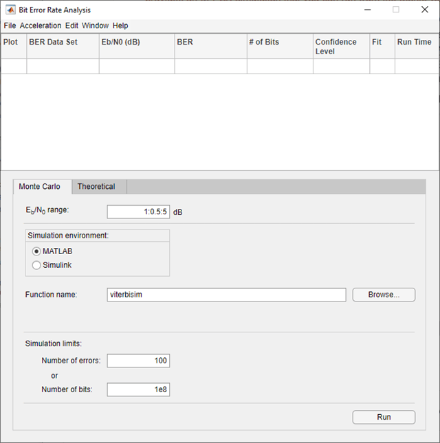
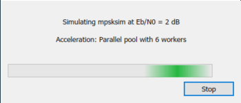
On the Monte Carlo tab, set the Eb/N0 range parameter to 1:1:5 and the Function name parameter to mpsksim.

Open the mpsksim function for editing, set M=2, and save the changed file.
Run the mpsksim.m function as configured by clicking Run on the Monte Carlo tab in the app.
After the app simulates the set of Eb/N0 points, update the name of the BER data set results by selecting simulation0 in the BER Data Set field and typing M=2 to rename the set of results. The legend on the BER figure updates the label to M=2.


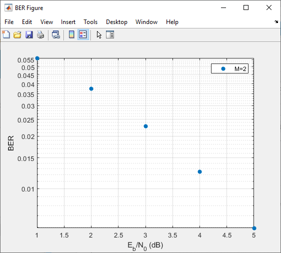
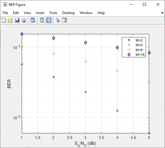
Update the value for M in the mpsksim function, repeating this process for M = 4, 8, and 16. For example, these figures of the Bit Error Rate Analysis app and BER Figure window show results for varying M values.

Parallel SNR Sweep Using Bit Error Rate Analysis App
The default configuration for the Monte Carlo processing of the Bit Error Rate Analysis app automatically uses parallel pool processing to process individual Eb/N0 points when you have the Parallel Computing Toolbox™ software but for the processing of your simulation code:
-
Any
parforfunction loops in your simulation code execute as standardforloops. -
Any
parfeval(Parallel Computing Toolbox) function calls in your simulation code execute serially. -
Any
spmd(Parallel Computing Toolbox) statement calls in your simulation code execute serially.
Copyright 2020 The MathWorks, Inc.
Prepare Simulink Model for Use with Bit Error Rate Analysis App
Use a Simulink simulation model to run in the Monte Carlo
tab of the Bit Error Rate Analysis app. Compare the BER performance
of the Simulink simulation results with theoretical BER results.
Prepare Model
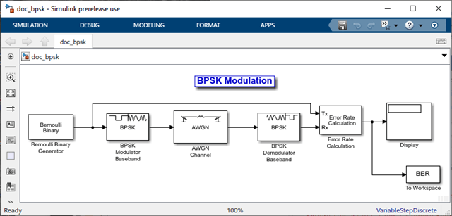
Open the model by entering doc_bpsk at the MATLAB command prompt.

Initialize parameters in the MATLAB workspace to avoid using undefined variables as block
parameters.
EbNo = 0;
maxNumErrs = 100;
maxNumBits = 1e8;
Ensure that the Bit Error Rate Analysis app uses the correct
amount of noise each time it runs the simulation, by opening the dialog box
for the AWGN Channel block and verifying
that the Es/No parameter is set to
EbNo.
Note
For BPSK modulation,
Es/N0
is equivalent to
Eb/N0.
Ensure that the Bit Error Rate Analysis app uses the correct
stopping criteria for each iteration by:
-
Opening the dialog box for the Error Rate
Calculation block and verifying that
Target number of errors is set to
maxNumErrsand that Maximum
number of symbols is set to
maxNumBits. -
Verifying that the simulation stop time is set to
Inf.
Enable the Bit Error Rate Analysis app to access the BER
results that the Error Rate Calculation block computes, by
ensuring that the BER variable name parameter in the
app matches the Variable name parameter set in the
To Workspace block that connects to the output of the
Error Rate Calculation block.
Use Prepared Model
Run the doc_bpsk model in the Bit Error Rate
Analysis app.
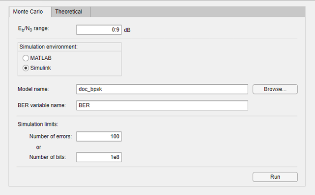
Open the Bit Error Rate Analysis app, and then select the
Monte Carlo tab.
Set these parameters to the specified values:
Eb/N0
range to 0:9, Simulation
environment to Simulink,
Function name to doc_bpsk,
Number of errors to 100, and
Number of bits to 1e8.

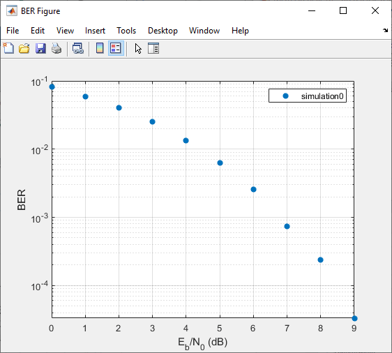
Click Run.
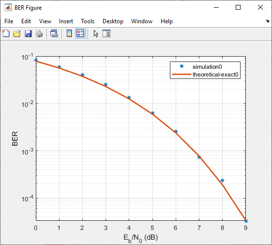
The Bit Error Rate Analysis app computes the results and then
plots them.

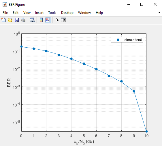
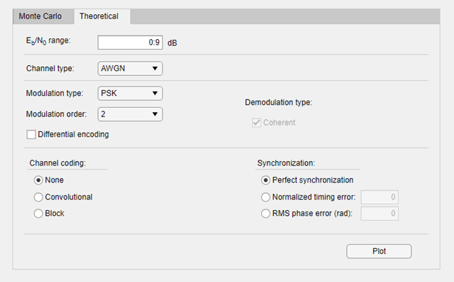
Compare these simulation results with the theoretical results, by clicking
the Theoretical tab in the Bit Error Rate
Analysis app and setting
Eb/N0
range to 0:9.

Click Plot.
The Bit Error Rate Analysis app plots the theoretical curve in
the BER Figure window along with the earlier simulation results.

Parameters
Theoretical
Eb/N0 range — Range of Eb/N0
values
0:18 (default) | scalar | vector
Range of
Eb/N0
values over which the BER is evaluated, specified as a scalar or vector.
Units are in dB.
Example: 5:10 specifies the evaluation of
Eb/N0
values over the range [5, 10] at 1 dB increments.
Channel type — Type of channel over which BER is evaluated
AWGN (default) | Rayleigh | Rician
Type of channel over which the BER is evaluated, specified as
AWGN, Rayleigh, or
Rician. The
Rayleigh and
Rician options correspond to flat fading
channels.
Modulation type — Modulation type of communications link
PSK (default) | DPSK | OQPSK | PAM | QAM | FSK | MSK | CPFSK
Modulation type of the communications link, specified as
PSK, DPSK,
OQPSK, PAM,
QAM, FSK,
MSK, or
CPFSK.
Modulation order — Modulation order of communications link
2 (default) | 4 | 8 | 16 | 32 | 64
Modulation order of the communications link, specified as
2, 4,
8, 16,
32, or 64.
Differential encoding — Differential encoding of input data
off (default) | on
Select this parameter to enable differential encoding of the input
data.
Correlation coefficient — Correlation coefficient
0 (default) | real scalar in the range [-1, 1]
Correlation coefficient, specified as a real scalar in the range [-1,
1].
Dependencies
To enable this parameter, set Modulation type to
FSK.
Modulation index — Modulation index
0.5 (default) | positive real scalar
Modulation index, specified as a positive real scalar.
Dependencies
To enable this parameter, set Modulation type to
CPFSK.
Demodulation type — Coherent demodulation of input data
on (default) | off
-
Select this parameter to enable coherent demodulation of the
input data. -
Clear this parameter to enable noncoherent demodulation of the
input data.
Dependencies
To enable this parameter, set Modulation type to
FSK or
MSK.
Channel coding — Channel coding type used when estimating theoretical BER
None (default) | Convolutional | Block
Channel coding type used when estimating the theoretical BER, specified as
None, Convolutional, or
Block.
Synchronization — Synchronization error
Perfect synchronization (default) | Normalized timing error | RMS phase noise level
Synchronization error in the demodulation process, specified as
Perfect synchronization, Normalized
timing error, or RMS phase noise
(rad).
-
When you set Synchronization to
Perfect synchronization no synchronization
errors are encountered in the demodulation process. -
When you set Synchronization to
Normalized timing error, you can set the
normalized timing error as a scalar in the range [0, 0.5]. -
When you set Synchronization to RMS
phase noise (rad), you can set the RMS phase noise
level as a nonnegative scalar. Units are in radians
Dependencies
To enable this parameter, set Modulation type to
PSK, Modulation
order to 2, and
Channel coding to
None.
Decision method — Decoding decision method
Hard (default) | Soft
Decoding decision method used to decode the received data, specified as
Hard or
Soft.
Dependencies
To enable this parameter, set Channel coding to
Convolutional or set Channel
coding to Block and set
Coding type to
General.
Trellis — Convolutional code trellis
poly2trellis(7,[171 133]) (default) | structure
Convolutional code trellis, specified as a structure variable. You can
generate this structure by using the poly2trellis function.
Dependencies
To enable this parameter, set Channel coding to
Convolutional.
Coding type — Block coding type
General (default) | Hamming | Golay | Reed-Solomon
Block coding type used in the BER evaluation, specified as
General, Hamming,
Golay, or
Reed-Solomon.
Dependencies
To enable this parameter, set Channel coding to
Block.
N — Codeword length
positive integer
Codeword length, specified as a positive integer.
Dependencies
To enable this parameter, set Channel coding to
Block and set Coding type
to General.
K — Message length
positive integer
Message length, specified as a positive integer such that
K is less than N.
Dependencies
To enable this parameter, set Channel coding to
Block and set Coding type
to General.
dmin — Minimum distance of (N,K) block code
positive integer
Minimum distance of the (N,K)
block code, specified as a positive integer.
Dependencies
To enable this parameter, set Channel coding to
Block and set Coding type
to General.
Monte Carlo
Eb/N0 range — Range of Eb/N0
values
1:0.5:5 (default) | scalar | vector
Range of
Eb/N0
values over which the BER is evaluated, specified as a scalar or vector.
Units are in dB.
Example: 4:2:10 specifies evaluation of
Eb/N0
over the range [4, 10] at 2 dB increments.
Simulation environment — Simulation environment
MATLAB (default) | Simulink
Simulation environment, specified as MATLAB or
Simulink.
Function name — Name of MATLAB function
viterbisim (default)
Name of the MATLAB function for the app to run for the Monte Carlo
simulation.
Dependencies
To enable this parameter, set Simulation
environment to MATLAB.
Model name — Name of Simulink model
commgraycode (default)
Name of the Simulink model for the app to run for the Monte Carlo
simulation.
Dependencies
To enable this parameter, set Simulation
environment to Simulink.
BER variable name — Name of variable containing BER simulation data
grayBER (default)
Name of the variable containing the BER simulation data. To output the BER
simulation data to the MATLAB workspace, you can assign this variable name as the
Variable name parameter value in a To
Workspace block.
Dependencies
To enable this parameter, set the Simulation
environment to Simulink.
Number of errors — Number of errors to be measured before simulation stops
100 (default) | positive integer
Number of errors to be measured before the simulation stops, specified as
a positive integer. Typically, to produce an accurate BER estimate,100
measured errors are enough.
Number of bits — Number of bits to be processed before simulation stops
1e8 (default) | positive integer
Number of bits to be processed before the simulation stops, specified as a
positive integer. This parameter is used to prevent the simulation from
running too long.
Note
The Monte Carlo simulation stops when either the number of errors or
number of bits threshold is reached.
Tips
-
You can stop the simulation by clicking Stop on the Monte
Carlo Simulation dialog box.

Version History
Introduced before R2006a
expand all
R2020b: Semianalytic tab in the Bit Error Rate Analysis has been removed
The Semianalytic tab and functionality in the Bit Error
Rate Analysis app has been removed. To generate semianalytic BER results,
you can still use the semianalytic function.
For example, this code shows you how to use the semianalytic
function to programmatically generate semianalytic BER results for a BPSK-modulated
signal.
data = [0 1 1 0 0 1 1 1 1 0 1 1 0 0 0 0].';
bpskmod = comm.BPSKModulator
txSig = rectpulse(bpskmod(data),16);
rxSig = rectpulse(bpskmod(data),16); % Before receive filter
modType = ‘psk’;
modOrder = 2;
sps = 16; % samples per symbol
num = ones(16,1) / 16; % Filter numerator
den = 1 % Filter denominator
EbNo = 0:18; % dB
BER = semianalytic(txSig,rxSig,modType,modOrder,sps,num,den,EbNo);
semilogy(EbNo,BER)
This topic describes how to compute error statistics for various communications
systems.
Computation of Theoretical Error Statistics
The biterr function, discussed in the
Compute SERs and BERs Using Simulated Data section, can help you gather empirical error
statistics, but validating your results by comparing them to the theoretical error
statistics is good practice. For certain types of communications systems,
closed-form expressions exist for the computation of the bit error rate (BER) or an
approximate bound on the BER. The functions listed in this table compute the
closed-form expressions for the BER or a bound on it for the specified types of
communications systems.
| Type of Communications System | Function |
|---|---|
| Uncoded AWGN channel | berawgn
|
| Uncoded Rayleigh and Rician fading channel | berfading
|
| Coded AWGN channel | bercoding |
| Uncoded AWGN channel with imperfect synchronization | bersync
|
The analytical expressions used in these functions are discussed in
Analytical Expressions Used in BER Analysis. The reference pages of these functions also list
references to one or more books containing the closed-form expressions implemented
by the function.
Theoretical Performance Results
-
Plot Theoretical Error Rates
-
Compare Theoretical and Empirical Error Rates
Plot Theoretical Error Rates
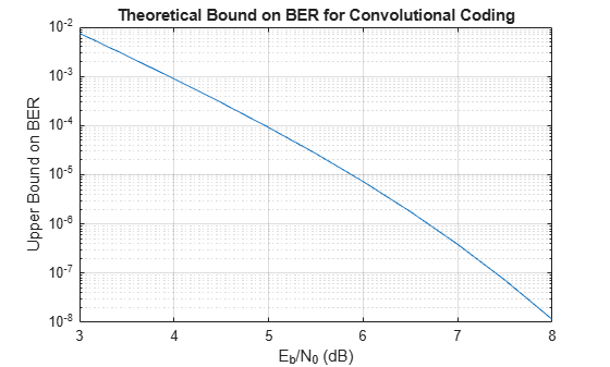
This example uses the bercoding function to compute upper bounds on BERs for convolutional coding with a soft-decision decoder.
coderate = 1/4; % Code rate
Create a structure, dspec, with information about the distance spectrum. Define the energy per bit to noise power spectral density ratio (Eb/N0) sweep range and generate the theoretical bound results.
dspec.dfree = 10; % Minimum free distance of code
dspec.weight = [1 0 4 0 12 0 32 0 80 0 192 0 448 0 1024 ...
    0 2304 0 5120 0]; % Distance spectrum of code
EbNo = 3:0.5:8;
berbound = bercoding(EbNo,'conv','soft',coderate,dspec);
Plot the theoretical bound results.
semilogy(EbNo,berbound)
xlabel('E_b/N_0 (dB)');
ylabel('Upper Bound on BER');
title('Theoretical Bound on BER for Convolutional Coding');
grid on;
Compare Theoretical and Empirical Error Rates
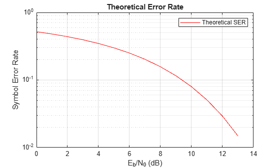
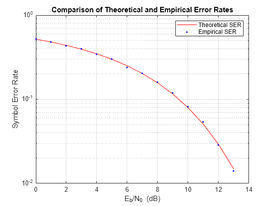
Using the berawgn function, compute the theoretical symbol error rates (SERs) for pulse amplitude modulation (PAM) over a range of Eb/N0 values. Simulate 8 PAM with an AWGN channel, and compute the empirical SERs. Compare the theoretical and then empirical SERs by plotting them on the same set of axes.
Compute and plot the theoretical SER using berawgn.
rng('default') % Set random number seed for repeatability
M = 8;
EbNo = 0:13;
[ber,ser] = berawgn(EbNo,'pam',M);

semilogy(EbNo,ser,'r');
legend('Theoretical SER');
title('Theoretical Error Rate');
xlabel('E_b/N_0 (dB)');
ylabel('Symbol Error Rate');
grid on;
Compute the empirical SER by simulating an 8 PAM communications system link. Define simulation parameters and preallocate variables needed for the results. As described in [1], because N0=2×(NVariance)2, add 3 dB to the Eb/N0 value when converting Eb/N0 values to SNR values.
n = 10000; % Number of symbols to process
k = log2(M); % Number of bits per symbol
snr = EbNo+3+10*log10(k); % In dB
ynoisy = zeros(n,length(snr));
z = zeros(n,length(snr));
errVec = zeros(3,length(EbNo));
Create an error rate calculator System object™ to compare decoded symbols to the original transmitted symbols.
errcalc = comm.ErrorRate;
Generate a random data message and apply PAM. Normalize the channel to the signal power. Loop the simulation to generate error rates over the range of SNR values.
x = randi([0 M-1],n,1); % Create message signal
y = pammod(x,M); % Modulate
signalpower = (real(y)'*real(y))/length(real(y));

for jj = 1:length(snr)
    reset(errcalc)
    ynoisy(:,jj) = awgn(real(y),snr(jj),'measured'); % Add AWGN
    z(:,jj) = pamdemod(complex(ynoisy(:,jj)),M); % Demodulate
    errVec(:,jj) = errcalc(x,z(:,jj)); % Compute SER from simulation
end
Compare the theoretical and empirical results.
hold on;
semilogy(EbNo,errVec(1,:),'b.');
legend('Theoretical SER','Empirical SER');
title('Comparison of Theoretical and Empirical Error Rates');
hold off;
Performance Results via Simulation
-
Section Overview
-
Compute SERs and BERs Using Simulated Data
Section Overview
This section describes how to compare the data messages that enter and leave
a communications system simulation and how to compute error statistics using the
Monte Carlo technique. Simulations can measure system performance by using the
data messages before transmission and after reception to compute the BER or SER
for a communications system. To explore physical layer components used to model
and simulate communications systems, see PHY Components.
Curve fitting can be useful when you have a small or imperfect data set but
want to plot a smooth curve for presentation purposes. To explore the use of
curve fitting when computing performance results via simulation, see the Curve Fitting for Error Rate Plots section.
Compute SERs and BERs Using Simulated Data
The example shows how to compute SERs and BERs using the biterr and symerr functions, respectively. The symerr function compares two sets of data and computes the number of symbol errors and the SER. The biterr function compares two sets of data and computes the number of bit errors and the BER. An error is a discrepancy between corresponding points in the two sets of data.
The two sets of data typically represent messages entering a transmitter and recovered messages leaving a receiver. You can also compare data entering and leaving other parts of your communications system (for example, data entering an encoder and data leaving a decoder).
If your communications system uses several bits to represent one symbol, counting symbol errors is different from counting bit errors. In either the symbol- or bit-counting case, the error rate is the number of errors divided by the total number of transmitted symbols or bits, respectively.
Typically, simulating enough data to produce at least 100 errors provides accurate error rate results. If the error rate is very small (for example, 10-6 or less), using the semianalytic technique might compute the result more quickly than using a simulation-only approach. For more information, see the Performance Results via Semianalytic Technique section.
Compute Error Rates
Use the symerr function to compute the SERs for a noisy linear block code. Apply no digital modulation, so that each symbol contains a single bit. When each symbol is a single bit, the symbol errors and bit errors are the same.
After artificially adding noise to the encoded message, compare the resulting noisy code to the original code. Then, decode and compare the decoded message to the original message.
m = 3; % Set parameters for Hamming code
n = 2^m-1;
k = n-m;
msg = randi([0 1],k*200,1); % Specify 200 messages of k bits each
code = encode(msg,n,k,'hamming');
codenoisy = bsc(code,0.95); % Add noise
newmsg = decode(codenoisy,n,k,'hamming'); % Decode and correct errors
Compute the SERs.
[~,noisyVec] = symerr(code,codenoisy);
[~,decodedVec] = symerr(msg,newmsg);
The error rate decreases after decoding because the Hamming decoder correct errors based on the error-correcting capability of the decoder configuration. Because random number generators produce the message and noise is added, results vary from run to run. Display the SERs.
disp(['SER in the received code: ',num2str(noisyVec(1))])
SER in the received code: 0.94571
disp(['SER after decoding: ',num2str(decodedVec(1))])
SER after decoding: 0.9675
Comparing SER and BER
These commands show the difference between symbol errors and bit errors in various situations.
Create two three-element decimal vectors and show the binary representation. The vector a contains three 2-bit symbols, and the vector b contains three 3-bit symbols.
bpi = 3; % Bits per integer
a = [1 2 3];
b = [1 4 4];
int2bit(a,bpi)
ans = 3×3

     0     0     0
     0     1     1
     1     0     1
ans = 3×3

     0     1     1
     0     0     0
     1     0     0
Compare the binary values of the two vectors and compute the number of errors and the error rate by using the biterr and symerr functions.
format rat % Display fractions instead of decimals
[snum,srate] = symerr(a,b)
snum is 2 because the second and third entries have bit differences. srate is 2/3 because the total number of symbols is 3.
[bnum,brate] = biterr(a,b)
bnum is 5 because the second entries differ in two bits, and the third entries differ in three bits. brate is 5/9 because the total number of bits is 9. By definition, the total number of bits is the number of entries in a for symbol error computations or b for bit error computations times the maximum number of bits among all entries of a and b, respectively.
Performance Results via Semianalytic Technique
The technique described in the Performance Results via Simulation
section can work for a large variety of communications systems but can be
prohibitively time-consuming for small error rates (for example,
10-6 or less). The semianalytic technique is an
alternative way to compute error rates. The semianalytic technique can produce
results faster than a nonanalytic method that uses simulated data.
For more information on implementing the semianalytic technique using a
combination of simulation and analysis to determine the error rate of a
communications system, see the semianalytic function.
Error Rate Plots
-
Section Overview
-
Creation of Error Rate Plots Using
semilogy
Function -
Curve Fitting for Error Rate Plots
-
Use Curve Fitting on Error Rate Plot
Section Overview
Error rate plots can be useful when examining the performance of a
communications system and are often included in publications. This section
discusses and demonstrates tools you can use to create error rate plots, modify
them to suit your needs, and perform curve fitting on the error rate data and
the plots.
Creation of Error Rate Plots Using semilogy Function
In many error rate plots, the horizontal axis indicates
Eb/N0
values in dB, and the vertical axis indicates the error rate using a logarithmic
(base 10) scale. For examples that create such a plot using the semilogy function, see Compare Theoretical and Empirical Error Rates and Plot Theoretical Error Rates.
Curve Fitting for Error Rate Plots
Curve fitting can be useful when you have a small or imperfect data set but
want to plot a smooth curve for presentation purposes. The berfit function includes
curve-fitting capabilities that help your analysis when the empirical data
describes error rates at different
Eb/N0
values. This function enables you to:
-
Customize various relevant aspects of the curve-fitting process, such
as a list of selections for the type of closed-form function used to
generate the fit. -
Plot empirical data along with a curve that
berfitfits to the
data. -
Interpolate points on the fitted curve between
Eb/N0
values in your empirical data set to smooth the plot. -
Collect relevant information about the fit, such as the numerical
values of points along the fitted curve and the coefficients of the fit
expression.
Note
The berfit function is
intended for curve fitting or interpolation, not extrapolation.
Extrapolating BER data beyond an order of magnitude below the smallest
empirical BER value is inherently unreliable.
Use Curve Fitting on Error Rate Plot
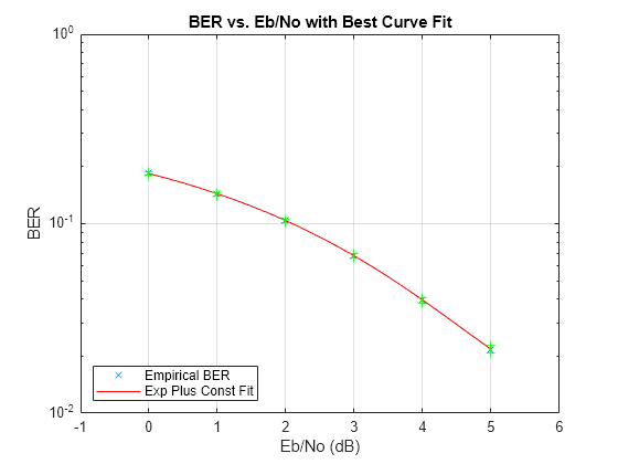
This example simulates a simple differential binary phase shift keying (DBPSK) communications system and plots error rate data for a series of Eb/N0 values. It uses the berfit and berconfint functions to fit a curve to a set of empirical error rates.
Initialize Simulation Parameters
Specify the input signal message length, modulation order, range of Eb/N0 values to simulate, and the minimum number of errors that must occur before the simulation computes an error rate for a given Eb/N0 value. Preallocate variables for final results and interim results.
Typically, for statistically accurate error rate results, the minimum number of errors must be on the order of 100. This simulation uses a small number of errors to shorten the run time and to illustrate how curve fitting can smooth a set of results.
siglen = 100000; % Number of bits in each trial
M = 2; % DBPSK is binary
EbN0vec = 0:5; % Vector of EbN0 values
minnumerr = 5; % Compute BER after only 5 errors occur
numEbN0 = length(EbN0vec); % Number of EbN0 values

ber = zeros(1,numEbN0); % Final BER values
berVec = zeros(3,numEbN0); % Updated BER values
intv = cell(1,numEbN0); % Cell array of confidence intervals
Create an error rate calculator System object™.
errorCalc = comm.ErrorRate;
Loop the Simulation
Simulate the DBPSK-modulated communications system and compute the BER using a for loop to vary the Eb/N0 value. The inner while loop ensures that a minimum number of bit errors occur for each Eb/N0 value. Error rate statistics are saved for each Eb/N0 value and used later in this example when curve fitting and plotting.
for jj = 1:numEbN0
    EbN0 = EbN0vec(jj);
    snr = EbN0; % For binary modulation SNR = EbN0
    reset(errorCalc)

    while (berVec(2,jj) < minnumerr)
        msg = randi([0,M-1],siglen,1); % Generate message sequence
        txsig = dpskmod(msg,M); % Modulate
        rxsig = awgn(txsig,snr,'measured'); % Add noise
        decodmsg = dpskdemod(rxsig,M); % Demodulate
        berVec(:,jj) = errorCalc(msg,decodmsg); % Calculate BER
    end
Use the berconfint function to compute the error rate at a 98% confidence interval for the Eb/N0 values.
    [ber(jj),intv1] = berconfint(berVec(2,jj),berVec(3,jj),0.98);
    intv{jj} = intv1;
    disp(['EbN0 = ' num2str(EbN0) ' dB, ' num2str(berVec(2,jj)) ...
        ' errors, BER = ' num2str(ber(jj))])
end
EbN0 = 0 dB, 18392 errors, BER = 0.18392
EbN0 = 1 dB, 14307 errors, BER = 0.14307
EbN0 = 2 dB, 10190 errors, BER = 0.1019
EbN0 = 3 dB, 6940 errors, BER = 0.0694
EbN0 = 4 dB, 4151 errors, BER = 0.04151
EbN0 = 5 dB, 2098 errors, BER = 0.02098
Use the berfit function to plot the best fitted curve, interpolating between BER points to get a smooth plot. Add confidence intervals to the plot.
fitEbN0 = EbN0vec(1):0.25:EbN0vec(end); % Interpolation values
berfit(EbN0vec,ber,fitEbN0);
hold on;
for jj=1:numEbN0
    semilogy([EbN0vec(jj) EbN0vec(jj)],intv{jj},'g-+');
end
hold off;
See Also
Apps
- Bit Error Rate Analysis
Functions
berawgn|bercoding|berconfint|berfading|berfit|bersync
Related Topics
- Analyze Performance with Bit Error Rate Analysis App
- Analytical Expressions Used in BER Analysis
Анализируйте эффективность BER систем связи
Описание
Приложение Bit Error Rate Analysis вычисляет частоту ошибок по битам (BER) в зависимости от энергии на бит к отношению спектральной плотности мощности шума (E b/N0). Используя это приложение, вы можете:
-
Сгенерируйте данные о BER для системы связи и анализируйте использование эффективности:
-
Симуляции Монте-Карло MATLAB® функции и Simulink® модели.
-
Теоретические выражения закрытой формы для выбранных типов систем связи.
-
Запустите системы, содержавшиеся в функциях симуляции MATLAB или моделях Simulink. После того, как вы создаете функцию или модель, которая симулирует систему, приложение Bit Error Rate Analysis выполняет итерации по вашему выбору значений E b/N0 и собирает результаты.
-
-
Постройте один или несколько наборов данных BER на одном наборе осей. Можно графически сравнить данные моделирования с теоретическими результатами или данные моделирования от ряда моделей системы связи.
-
Соответствуйте кривой к набору данных моделирования.
-
Постройте доверительные уровни данных моделирования.
-
Отправьте данные о BER в рабочее пространство MATLAB или в файл для последующей обработки.
Для получения дополнительной информации смотрите Использование Приложение Bit Error Rate Analysis.
Откройте приложение Bit Error Rate Analysis
-
Панель инструментов MATLAB: На вкладке Apps, под Signal Processing and Communications, кликают по значку приложения.
-
Командная строка MATLAB: Войти
bertool.
Примеры
развернуть все
Вычислите BER Используя теоретическую вкладку
Сгенерируйте теоретическую оценку эффективности BER для 16-QAM ссылки в AWGN.
Откройте приложение Bit Error Rate Analysis.

На вкладке Theoretical, установленной эти параметры на заданные значения: Eb/N0 range к 0:10, Modulation type к QAM, и Modulation order к 16.
Постройте кривую BER путем нажатия на Plot.

Вычислите BER Используя симуляцию вкладки и функции MATLAB Монте-Карло
Симулируйте BER при помощи пользовательской функции MATLAB. По умолчанию приложение использует viterbisim.m симуляция.
Откройте приложение Bit Error Rate Analysis.
На вкладке Monte Carlo, установленной параметр Eb/N0 range на 1:.5:6. Запустите симуляцию и постройте предполагаемые значения BER путем нажатия на Run.
На вкладке Theoretical, набор Eb/N0 range к 1:6 и набор Modulation order к 4. Включите сверточное кодирование путем выбора Convolutional. Нажмите Plot, чтобы добавить теоретическую верхнюю границу кривой BER к графику.
Подготовьте функцию MATLAB к использованию в приложении Bit Error Rate Analysis
Добавьте код в шаблон функции симуляции, данный в Шаблоне для темы Функции Симуляции, чтобы запуститься во вкладке Monte Carlo Bit Error Rate Analysis.
Подготовьте функцию
Скопируйте шаблон с Шаблона для темы Функции Симуляции в новый файл MATLAB в редакторе MATLAB. Сохраните файл в папке на своем пути MATLAB, с помощью имени файла bertool_simfcn.
Поместите строки кода, которые инициализируют параметры или создают объекты, используемые в симуляции в разделе шаблона, отмеченном Set up initial parameters. Эта симуляция кодированных карт переменные к входным параметрам шаблона. Например, snr карты к EbNo.
% Set up initial parameters.
siglen = 1000; % Number of bits in each trial
M = 2;         % DBPSK is binary
snr = EbNo;    % Because of binary modulation

% Create an ErrorRate calculator System object to compare
% decoded symbols to the original transmitted symbols.
errorCalc = comm.ErrorRate;
Поместите код для базовых задач симуляции в разделе шаблона отметил Proceed with simulation. Этот код включает базовые задачи симуляции, после того, как вся настройка работает, был выполнен.
    msg = randi([0,M-1],siglen,1); % Generate message sequence
    txsig = dpskmod(msg,M);        % Modulate
    hChan.SignalPower = ...        % Calculate and assign signal power
        (txsig'*txsig)/length(txsig);
    rxsig = awgn(txsig,snr,'measured'); % Add noise
    decodmsg = dpskdemod(rxsig,M);      % Demodulate
    berVec = errorCalc(msg,decodmsg);   % Calculate BER
    totErr = totErr + berVec(2);
    numBits = numBits + berVec(3);
После того, как вы вставляете эти две секции кода в шаблон, bertool_simfcn функция совместима с приложением Bit Error Rate Analysis. Получившийся код напоминает этот сегмент кода.
function [ber,numBits] = bertool_simfcn(EbNo,maxNumErrs,maxNumBits,varargin)
%
%   See also BERTOOL and VITERBISIM.

% Copyright 2020 The MathWorks, Inc.

% Initialize variables related to exit criteria.
totErr = 0;  % Number of errors observed
numBits = 0; % Number of bits processed

% --- Set up the simulation parameters. ---
% --- INSERT YOUR CODE HERE.
% Set up initial parameters.
siglen = 1000; % Number of bits in each trial
M = 2;         % DBPSK is binary.
snr = EbNo;    % Because of binary modulation
% Create an ErrorRate calculator System object to compare
% decoded symbols to the original transmitted symbols.
errorCalc = comm.ErrorRate;

% Simulate until the number of errors exceeds maxNumErrs
% or the number of bits processed exceeds maxNumBits.
while((totErr < maxNumErrs) && (numBits < maxNumBits))

    % Check if the user clicked the Stop button of BERTool.
    if isBERToolSimulationStopped(varargin{:})
      break
    end

    % --- Proceed with the simulation.
    % --- Update totErr and numBits.
    % --- INSERT YOUR CODE HERE.
    msg = randi([0,M-1],siglen,1); % Generate message sequence
    txsig = dpskmod(msg,M);        % Modulate
    hChan.SignalPower = ...        % Calculate and assign signal power
        (txsig'*txsig)/length(txsig);
    rxsig = awgn(txsig,snr,'measured'); % Add noise
    decodmsg = dpskdemod(rxsig,M);      % Demodulate
    berVec = errorCalc(msg,decodmsg);   % Calculate BER
    totErr = totErr + berVec(2);
    numBits = numBits + berVec(3);
end % End of loop

% Compute the BER.
ber = totErr/numBits;
Функция имеет входные параметры, чтобы задать приложение и скаляры для EbNo, maxNumErrs, и maxNumBits это обеспечивается приложением. Приложение Bit Error Rate Analysis является входом, потому что функция контролирует и отвечает на команду остановки в приложении. bertool_simfcn функция исключает код, связанный с графическим выводом, аппроксимированием кривыми и доверительными интервалами, потому что приложение Bit Error Rate Analysis позволяет вам сделать подобные задачи в интерактивном режиме без написания кода.
Используйте подготовленную функцию
Запустите bertool_simfcn в приложении Bit Error Rate Analysis.
Откройте приложение Bit Error Rate Analysis, и затем выберите вкладку Monte Carlo.
Установите эти параметры на заданные значения: Eb/N0 range к 0:10, Simulation environment к MATLAB, Function name к bertool_simfcn, Number of errors к 5, и Number of bits к 1e8.
Нажмите Run.
Приложение Bit Error Rate Analysis вычисляет результаты и затем строит их. В этом случае результаты, кажется, не падают вдоль плавной кривой, потому что симуляция потребовала только пяти ошибок для каждого значения в EbNo.

Соответствуйте кривой к серии точек в Окне рисунка BER путем выбора параметра Fit в средстве просмотра данных.

Приложение Bit Error Rate Analysis строит кривую по экспериментальным точкам, как показано в этом рисунке.
Вычислите развертки симуляции коэффициента ошибок Используя приложение Bit Error Rate Analysis
Используйте приложение Bit Error Rate Analysis, чтобы вычислить BER в зависимости от Eb/N0. Приложение анализирует эффективность или с симуляциями Монте-Карло функций MATLAB® и моделей Simulink® или с теоретическими выражениями закрытой формы для выбранных типов систем связи. Код в функции mpsksim.m предоставляет симуляцию M-PSK, которую можно запустить от вкладки Monte Carlo приложения.
Откройте приложение Bit Error Rate Analysis от вкладки Apps или путем выполнения bertool функция в командном окне MATLAB®.

На вкладке Monte Carlo, набор Eb/N0 параметр области значений к 1:1:5 и параметр Имени функции к mpsksim.

Откройте mpsksim функция для редактирования, набор M=2, и сохраните измененный файл.
Запустите mpsksim.m функционируйте, как сконфигурировано путем нажатия, работает на вкладке Monte Carlo в приложении.
После того, как приложение симулирует набор Eb/N0 точки, обновите имя результатов набора данных BER путем выбора simulation0 в поле BER Data Set и вводе M=2 переименовать набор результатов. Легенда на фигуре BER обновляет метку к M=2.


Обновите значение для M в mpsksim функция, повторяя этот процесс для M= 4 , 8, и 16. Например, эти рисунки приложения Bit Error Rate Analysis и Окна рисунка BER показывают результаты для различного M значения.


Параллельная развертка ОСШ Используя приложение Bit Error Rate Analysis
Настройка по умолчанию для обработки Монте-Карло приложения Bit Error Rate Analysis автоматически использует параллельную обработку пула, чтобы обработать индивидуума Eb/N0 точки, когда у вас есть программное обеспечение Parallel Computing Toolbox™, но для обработки вашего кода симуляции:
-
Любой
parforфункциональные циклы в вашем коде симуляции выполняются как стандартныйforциклы. -
Любой
parfeval(Parallel Computing Toolbox) вызовы функции в вашем коде симуляции выполняется последовательно. -
Любой
spmdВызовы оператора (Parallel Computing Toolbox) в вашем коде симуляции выполняются последовательно.

Подготовьте модель Simulink к использованию с приложением Bit Error Rate Analysis
Используйте имитационную модель Simulink, чтобы запуститься во вкладке Monte Carlo приложения Bit Error Rate Analysis. Сравните эффективность BER результатов симуляции Simulink теоретическими результатами BER.
Подготовьте модель
Откройте модель путем ввода doc_bpsk в командной строке MATLAB.
Инициализируйте параметры в рабочем пространстве MATLAB, чтобы избегать использования неопределенных переменных как параметров блоков.
EbNo = 0;
maxNumErrs = 100;
maxNumBits = 1e8;
Убедитесь, что приложение Bit Error Rate Analysis использует правильное количество шума каждый раз, когда это запускает симуляцию путем открытия диалогового окна для блока AWGN Channel и проверки, что параметр Es/No устанавливается на EbNo.
Примечание
Для модуляции BPSK E s/N0 эквивалентен E b/N0.
Убедитесь, что приложение Bit Error Rate Analysis использует правильный критерий остановки для каждой итерации:
-
Открытие диалогового окна для блока Error Rate Calculation и проверка, что Target number of errors установлен в
maxNumErrsи что Maximum number of symbols установлен вmaxNumBits. -
Проверка, что время остановки симуляции установлено в
Inf.
Позвольте приложению Bit Error Rate Analysis получить доступ к результатам BER, которые блок Error Rate Calculation вычисляет путем гарантирования, что параметр BER variable name в приложении совпадает с набором параметров Variable name в блоке To Workspace (Simulink), который соединяется с выходом блока Error Rate Calculation.
Совет
Больше чем один блок To Workspace существует. Выберите блок To Workspace из подбиблиотеки DSP System Toolbox™ / Sinks.
Используйте подготовленную модель
Запустите doc_bpsk модель в приложении Bit Error Rate Analysis.
Откройте приложение Bit Error Rate Analysis, и затем выберите вкладку Monte Carlo.
Установите эти параметры на заданные значения: Eb/N0 range к 0:9, Simulation environment к Simulink, Function name к doc_bpsk, Number of errors к 100, и Number of bits к 1e8.
Нажмите Run.
Приложение Bit Error Rate Analysis вычисляет результаты и затем строит их.
Сравните эти результаты симуляции с теоретическими результатами путем нажатия на вкладку Theoretical в приложении Bit Error Rate Analysis и установке Eb/N0 range к 0:9.
Нажмите Plot.
Приложение Bit Error Rate Analysis строит теоретическую кривую в Окне рисунка BER наряду с более ранними результатами симуляции.
Параметры
Теоретический
Eb/N0 range — Область значений значений E b/N0
0:18
Область значений значений E b/N0, по которым BER оценен в виде скаляра или вектора. Величины в дБ.
Пример: 5:10 задает оценку значений E b/N0 в области значений [5, 10] в шаге на 1 дБ.
Channel type — Тип канала, по которому оценен BER
AWGN (значение по умолчанию) | Rayleigh | Rician
Тип канала, по которому BER оценен в виде AWGN, Rayleigh, или Rician. Rayleigh и Rician опции соответствуют плоским исчезающим каналам.
Modulation type — Тип модуляции линии связи
PSK (значение по умолчанию) | DPSK | OQPSK | PAM | QAM | FSK | MSK | CPFSK
Тип модуляции линии связи в виде PSK, DPSK, OQPSK, PAM, QAM, FSK, MSK, или CPFSK.
Modulation order — Порядок модуляции линии связи
2 4| 8
Порядок модуляции линии связи в виде 2, 4, 8, 16, 32, или 64.
Differential encoding — Дифференциальное кодирование входных данных
off (значение по умолчанию) | on
Выберите этот параметр, чтобы включить дифференциальное кодирование входных данных.
Correlation coefficient Коэффициент корреляции
0
Коэффициент корреляции в виде действительного скаляра в области значений [-1, 1].
Зависимости
Чтобы включить этот параметр, установите Modulation type на FSK.
Modulation index — Индекс модуляции
0.5
Индекс модуляции в виде положительного действительного скаляра.
Зависимости
Чтобы включить этот параметр, установите Modulation type на CPFSK.
Demodulation type — Когерентная демодуляция входных данных
on (значение по умолчанию) | off
-
Выберите этот параметр, чтобы включить когерентную демодуляцию входных данных.
-
Очистите этот параметр, чтобы включить некогерентную демодуляцию входных данных.
Зависимости
Чтобы включить этот параметр, установите Modulation type на FSK или MSK.
Channel coding — Тип кодирования канала используется при оценке теоретического BER
None (значение по умолчанию) | Convolutional | Block
Тип кодирования канала, используемый при оценке теоретического BER в виде None, Convolutional или Block.
Synchronization — Ошибка синхронизации
Perfect synchronization (значение по умолчанию) | Normalized timing error | RMS phase noise level
Ошибка синхронизации в процессе демодуляции в виде Perfect synchronization, Normalized timing error или RMS phase noise (rad).
-
Когда вы устанавливаете Synchronization на Perfect synchronization, ни с какими ошибками синхронизации не сталкиваются в процессе демодуляции.
-
Когда вы устанавливаете Synchronization на Normalized timing error, можно установить нормированную ошибку синхронизации как скаляр в области значений [0, 0.5].
-
Когда вы устанавливаете Synchronization на RMS phase noise (rad), можно установить уровень шума фазы RMS как неотрицательный скаляр. Модули исчисляются в радианах
Зависимости
Чтобы включить этот параметр, установите Modulation type на PSK, Modulation order к 2, и Channel coding к None.
Decision method — Декодирование метода решения
Hard (значение по умолчанию) | Soft
Декодирование метода решения раньше декодировало принятые данные в виде Hard или Soft.
Зависимости
Чтобы включить этот параметр, установите Channel coding на Convolutional или установите Channel coding на Block и установите Coding type на General.
Trellis — Решетка сверточного кода
poly2trellis(7,[171 133]) (значение по умолчанию) | структура
Решетка сверточного кода в виде переменной структуры. Можно сгенерировать эту структуру при помощи poly2trellis функция.
Зависимости
Чтобы включить этот параметр, установите Channel coding на Convolutional.
Coding type — Тип блочного кодирования
General (значение по умолчанию) | Hamming | Golay | Reed-Solomon
Тип блочного кодирования используется в оценке BER в виде General, Hamming, Golay, или Reed-Solomon.
Зависимости
Чтобы включить этот параметр, установите Channel coding на Block.
N — Длина кодовой комбинации
положительное целое число
Длина кодовой комбинации в виде положительного целого числа.
Зависимости
Чтобы включить этот параметр, установите Channel coding на Block и установите Coding type на General.
K — Передайте длину
положительное целое число
Передайте длину в виде положительного целого числа, таким образом, что K меньше N.
Зависимости
Чтобы включить этот параметр, установите Channel coding на Block и установите Coding type на General.
dmin — Минимальное расстояние (N, K) блочный код
положительное целое число
Минимальное расстояние (N, K) блочный код в виде положительного целого числа.
Зависимости
Чтобы включить этот параметр, установите Channel coding на Block и установите Coding type на General.
Монте-Карло
Eb/N0 range — Область значений значений E b/N0
1:0.5:5
Область значений значений E b/N0, по которым BER оценен в виде скаляра или вектора. Величины в дБ.
Пример: 4:2:10 задает оценку E b/N0 в области значений [4, 10] в шаге на 2 дБ.
Simulation environment — Среда симуляции
MATLAB (значение по умолчанию) | Simulink
Среда симуляции в виде MATLAB или Simulink.
Function name — Имя функции MATLAB
viterbisim (значение по умолчанию)
Имя функции MATLAB для приложения, чтобы запуститься для симуляции Монте-Карло.
Зависимости
Чтобы включить этот параметр, установите Simulation environment на MATLAB.
Model name — Имя модели Simulink
commgraycode (значение по умолчанию)
Имя модели Simulink для приложения, чтобы запуститься для симуляции Монте-Карло.
Зависимости
Чтобы включить этот параметр, установите Simulation environment на Simulink.
BER variable name — Имя переменных, содержащих данные моделирования BER
grayBER (значение по умолчанию)
Имя переменной, содержащей данные моделирования BER. Чтобы вывести данные моделирования BER к рабочему пространству MATLAB, можно присвоить это имя переменной как значение параметров Variable name в блоке To Workspace (Simulink).
Совет
Больше чем один блок To Workspace существует. Выберите блок To Workspace из подбиблиотеки DSP System Toolbox / Sinks.
Зависимости
Чтобы включить этот параметр, установите Simulation environment на Simulink.
Number of errors — Количество ошибок, которые будут измерены перед симуляцией, останавливается
100
Количество ошибок, которые будут измерены перед симуляцией, останавливается в виде положительного целого числа. Как правило, чтобы произвести точную оценку BER, 100 измеренных ошибок достаточно.
Number of bits — Количество битов, которые будут обработаны перед симуляцией, останавливается
1e8 (значение по умолчанию) | положительное целое число
Количество битов, которые будут обработаны перед симуляцией, останавливается в виде положительного целого числа. Этот параметр используется, чтобы препятствовать тому, чтобы симуляция запускалась слишком долго.
Примечание
Симуляция Монте-Карло останавливается, когда или количество ошибок или количество порога битов достигнуты.
Советы
-
Можно остановить симуляцию путем нажатия на Stop на диалоговом окне Monte Carlo Simulation.
Вопросы совместимости
развернуть все
Полуаналитическая вкладка в Bit Error Rate Analysis была удалена
Поведение изменяется в R2020b
Вкладка Semianalytic и функциональность в приложении Bit Error Rate Analysis были удалены. Чтобы сгенерировать полуаналитические результаты BER, можно все еще использовать semianalytic функция.
Например, этот код показывает вам, как использовать semianalytic функционируйте, чтобы программно сгенерировать полуаналитические результаты BER для модулируемого BPSK сигнала.
data = [0 1 1 0 0 1 1 1 1 0 1 1 0 0 0 0].';
bpskmod = comm.BPSKModulator
txSig = rectpulse(bpskmod(data),16);
rxSig = rectpulse(bpskmod(data),16); % Before receive filter
modType = ‘psk’;
modOrder = 2;
sps = 16; % samples per symbol
num = ones(16,1) / 16; % Filter numerator
den = 1 % Filter denominator
EbNo = 0:18; % dB
BER = semianalytic(txSig,rxSig,modType,modOrder,sps,num,den,EbNo);
semilogy(EbNo,BER)
Представлено до R2006a
Содержание
- Bit error rate analysis tool matlab
- Computation of Theoretical Error Statistics
- Theoretical Performance Results
- Plot Theoretical Error Rates
- Compare Theoretical and Empirical Error Rates
- Performance Results via Simulation
- Section Overview
- Compute SERs and BERs Using Simulated Data
- Bit Error Rate Analysis
- Description
- Open the Bit Error Rate Analysis App
- Examples
- Compute BER Using Theoretical Tab
- Compute BER Using Monte Carlo Tab and MATLAB Function Simulation
- Prepare MATLAB Function for Use in Bit Error Rate Analysis App
- Bit error rate analysis tool matlab
- Computation of Theoretical Error Statistics
- Theoretical Performance Results
- Plot Theoretical Error Rates
- Compare Theoretical and Empirical Error Rates
- Performance Results via Simulation
- Section Overview
- Compute SERs and BERs Using Simulated Data
This topic describes how to compute error statistics for various communications systems.
Computation of Theoretical Error Statistics
The biterr function, discussed in the Compute SERs and BERs Using Simulated Data section, can help you gather empirical error statistics, but validating your results by comparing them to the theoretical error statistics is good practice. For certain types of communications systems, closed-form expressions exist for the computation of the bit error rate (BER) or an approximate bound on the BER. The functions listed in this table compute the closed-form expressions for the BER or a bound on it for the specified types of communications systems.
| Type of Communications System | Function |
|---|---|
| Uncoded AWGN channel | berawgn |
| Uncoded Rayleigh and Rician fading channel | berfading |
| Coded AWGN channel | bercoding |
| Uncoded AWGN channel with imperfect synchronization | bersync |
The analytical expressions used in these functions are discussed in Analytical Expressions Used in BER Analysis. The reference pages of these functions also list references to one or more books containing the closed-form expressions implemented by the function.
Theoretical Performance Results
Plot Theoretical Error Rates
This example uses the bercoding function to compute upper bounds on BERs for convolutional coding with a soft-decision decoder.
Create a structure, dspec , with information about the distance spectrum. Define the energy per bit to noise power spectral density ratio ( E b / N 0 ) sweep range and generate the theoretical bound results.
Plot the theoretical bound results.
Compare Theoretical and Empirical Error Rates
Using the berawgn function, compute the theoretical symbol error rates (SERs) for pulse amplitude modulation (PAM) over a range of E b / N 0 values. Simulate 8 PAM with an AWGN channel, and compute the empirical SERs. Compare the theoretical and then empirical SERs by plotting them on the same set of axes.
Compute and plot the theoretical SER using berawgn .
Compute the empirical SER by simulating an 8 PAM communications system link. Define simulation parameters and preallocate variables needed for the results. As described in [1], because N 0 = 2 × ( N Variance ) 2 , add 3 dB to the E b / N 0 value when converting E b / N 0 values to SNR values.
Create an error rate calculator System object™ to compare decoded symbols to the original transmitted symbols.
Generate a random data message and apply PAM. Normalize the channel to the signal power. Loop the simulation to generate error rates over the range of SNR values.
Compare the theoretical and empirical results.
Performance Results via Simulation
Section Overview
This section describes how to compare the data messages that enter and leave a communications system simulation and how to compute error statistics using the Monte Carlo technique. Simulations can measure system performance by using the data messages before transmission and after reception to compute the BER or SER for a communications system. To explore physical layer components used to model and simulate communications systems, see PHY Components.
Curve fitting can be useful when you have a small or imperfect data set but want to plot a smooth curve for presentation purposes. To explore the use of curve fitting when computing performance results via simulation, see the Curve Fitting for Error Rate Plots section.
Compute SERs and BERs Using Simulated Data
The example shows how to compute SERs and BERs using the biterr and symerr functions, respectively. The symerr function compares two sets of data and computes the number of symbol errors and the SER. The biterr function compares two sets of data and computes the number of bit errors and the BER. An error is a discrepancy between corresponding points in the two sets of data.
The two sets of data typically represent messages entering a transmitter and recovered messages leaving a receiver. You can also compare data entering and leaving other parts of your communications system (for example, data entering an encoder and data leaving a decoder).
If your communications system uses several bits to represent one symbol, counting symbol errors is different from counting bit errors. In either the symbol- or bit-counting case, the error rate is the number of errors divided by the total number of transmitted symbols or bits, respectively.
Typically, simulating enough data to produce at least 100 errors provides accurate error rate results. If the error rate is very small (for example, 10 — 6 or less), using the semianalytic technique might compute the result more quickly than using a simulation-only approach. For more information, see the Performance Results via Semianalytic Technique section.
Compute Error Rates
Use the symerr function to compute the SERs for a noisy linear block code. Apply no digital modulation, so that each symbol contains a single bit. When each symbol is a single bit, the symbol errors and bit errors are the same.
After artificially adding noise to the encoded message, compare the resulting noisy code to the original code. Then, decode and compare the decoded message to the original message.
Compute the SERs.
The error rate decreases after decoding because the Hamming decoder correct errors based on the error-correcting capability of the decoder configuration. Because random number generators produce the message and noise is added, results vary from run to run. Display the SERs.
Источник
Bit Error Rate Analysis
Analyze BER performance of communications systems
Description
The Bit Error Rate Analysis app calculates the bit error rate (BER) as a function of the energy per bit to noise power spectral density ratio ( Eb/ N). Using this app, you can:
Generate BER data for a communications system and analyze performance using:
Monte Carlo simulations of MATLAB ® functions and Simulink ® models.
Theoretical closed-form expressions for selected types of communications systems.
Run systems contained in MATLAB simulation functions or Simulink models. After you create a function or model that simulates the system, the Bit Error Rate Analysis app iterates over your choice of Eb/ N values and collects the results.
Plot one or more BER data sets on a single set of axes. You can graphically compare simulation data with theoretical results or simulation data from a series of communications system models.
Fit a curve to a set of simulation data.
Plot confidence levels of simulation data.
Send BER data to the MATLAB workspace or to a file for further processing.
Open the Bit Error Rate Analysis App
MATLAB Toolstrip: On the Apps tab, under Signal Processing and Communications, click the app icon.
MATLAB command prompt: Enter bertool .
Examples
Compute BER Using Theoretical Tab
Generate a theoretical estimate of BER performance for a 16-QAM link in AWGN.
Open the Bit Error Rate Analysis app.
On the Theoretical tab, set these parameters to the specified values: Eb/N range to 0:10 , Modulation type to QAM , and Modulation order to 16 .
Plot the BER curve by clicking Plot.
Compute BER Using Monte Carlo Tab and MATLAB Function Simulation
Simulate the BER by using a custom MATLAB function. By default, the app uses the viterbisim.m simulation.
Open the Bit Error Rate Analysis app.
On the Monte Carlo tab, set the Eb/N range parameter to 1:.5:6 . Run the simulation and plot the estimated BER values by clicking Run.
On the Theoretical tab, set Eb/N range to 1:6 and set Modulation order to 4 . Enable convolutional coding by selecting Convolutional. Click Plot to add the theoretical upper bound of the BER curve to the plot.
Prepare MATLAB Function for Use in Bit Error Rate Analysis App
Add code to the simulation function template given in the Template for Simulation Function topic to run in the Monte Carlo tab of the Bit Error Rate Analysis.
Copy the template from the Template for Simulation Function topic into a new MATLAB file in the MATLAB Editor. Save the file in a folder on your MATLAB path, using the file name bertool_simfcn .
Place lines of code that initialize parameters or create objects used in the simulation in the template section marked Set up initial parameters . This code maps simulation variables to the template input arguments. For example, snr maps to EbNo .
Place the code for the core simulation tasks in the template section marked Proceed with simulation . This code includes the core simulation tasks, after all setup work has been performed.
After you insert these two code sections into the template, the bertool_simfcn function is compatible with the Bit Error Rate Analysis app. The resulting code resembles this code segment.
The function has inputs to specify the app and scalar quantities for EbNo , maxNumErrs , and maxNumBits that are provided by the app. The Bit Error Rate Analysis app is an input because the function monitors and responds to the stop command in the app. The bertool_simfcn function excludes code related to plotting, curve fitting, and confidence intervals because the Bit Error Rate Analysis app enables you to do similar tasks interactively without writing code.
Use Prepared Function
Run bertool_simfcn in the Bit Error Rate Analysis app.
Open the Bit Error Rate Analysis app, and then select the Monte Carlo tab.
Set these parameters to the specified values: Eb/N range to 0:10 , Simulation environment to MATLAB , Function name to bertool_simfcn , Number of errors to 5 , and Number of bits to 1e8 .
The Bit Error Rate Analysis app computes the results and then plots them. In this case, the results do not appear to fall along a smooth curve because the simulation required only five errors for each value in EbNo .
Fit a curve to the series of points in the BER Figure window, by selecting the Fit parameter in the data viewer.
The Bit Error Rate Analysis app plots the fitted curve, as shown in this figure.
Источник
This topic describes how to compute error statistics for various communications systems.
Computation of Theoretical Error Statistics
The biterr function, discussed in the Compute SERs and BERs Using Simulated Data section, can help you gather empirical error statistics, but validating your results by comparing them to the theoretical error statistics is good practice. For certain types of communications systems, closed-form expressions exist for the computation of the bit error rate (BER) or an approximate bound on the BER. The functions listed in this table compute the closed-form expressions for the BER or a bound on it for the specified types of communications systems.
| Type of Communications System | Function |
|---|---|
| Uncoded AWGN channel | berawgn |
| Uncoded Rayleigh and Rician fading channel | berfading |
| Coded AWGN channel | bercoding |
| Uncoded AWGN channel with imperfect synchronization | bersync |
The analytical expressions used in these functions are discussed in Analytical Expressions Used in BER Analysis. The reference pages of these functions also list references to one or more books containing the closed-form expressions implemented by the function.
Theoretical Performance Results
Plot Theoretical Error Rates
This example uses the bercoding function to compute upper bounds on BERs for convolutional coding with a soft-decision decoder.
Create a structure, dspec , with information about the distance spectrum. Define the energy per bit to noise power spectral density ratio ( E b / N 0 ) sweep range and generate the theoretical bound results.
Plot the theoretical bound results.
Compare Theoretical and Empirical Error Rates
Using the berawgn function, compute the theoretical symbol error rates (SERs) for pulse amplitude modulation (PAM) over a range of E b / N 0 values. Simulate 8 PAM with an AWGN channel, and compute the empirical SERs. Compare the theoretical and then empirical SERs by plotting them on the same set of axes.
Compute and plot the theoretical SER using berawgn .
Compute the empirical SER by simulating an 8 PAM communications system link. Define simulation parameters and preallocate variables needed for the results. As described in [1], because N 0 = 2 × ( N Variance ) 2 , add 3 dB to the E b / N 0 value when converting E b / N 0 values to SNR values.
Create an error rate calculator System object™ to compare decoded symbols to the original transmitted symbols.
Generate a random data message and apply PAM. Normalize the channel to the signal power. Loop the simulation to generate error rates over the range of SNR values.
Compare the theoretical and empirical results.
Performance Results via Simulation
Section Overview
This section describes how to compare the data messages that enter and leave a communications system simulation and how to compute error statistics using the Monte Carlo technique. Simulations can measure system performance by using the data messages before transmission and after reception to compute the BER or SER for a communications system. To explore physical layer components used to model and simulate communications systems, see PHY Components.
Curve fitting can be useful when you have a small or imperfect data set but want to plot a smooth curve for presentation purposes. To explore the use of curve fitting when computing performance results via simulation, see the Curve Fitting for Error Rate Plots section.
Compute SERs and BERs Using Simulated Data
The example shows how to compute SERs and BERs using the biterr and symerr functions, respectively. The symerr function compares two sets of data and computes the number of symbol errors and the SER. The biterr function compares two sets of data and computes the number of bit errors and the BER. An error is a discrepancy between corresponding points in the two sets of data.
The two sets of data typically represent messages entering a transmitter and recovered messages leaving a receiver. You can also compare data entering and leaving other parts of your communications system (for example, data entering an encoder and data leaving a decoder).
If your communications system uses several bits to represent one symbol, counting symbol errors is different from counting bit errors. In either the symbol- or bit-counting case, the error rate is the number of errors divided by the total number of transmitted symbols or bits, respectively.
Typically, simulating enough data to produce at least 100 errors provides accurate error rate results. If the error rate is very small (for example, 10 — 6 or less), using the semianalytic technique might compute the result more quickly than using a simulation-only approach. For more information, see the Performance Results via Semianalytic Technique section.
Compute Error Rates
Use the symerr function to compute the SERs for a noisy linear block code. Apply no digital modulation, so that each symbol contains a single bit. When each symbol is a single bit, the symbol errors and bit errors are the same.
After artificially adding noise to the encoded message, compare the resulting noisy code to the original code. Then, decode and compare the decoded message to the original message.
Compute the SERs.
The error rate decreases after decoding because the Hamming decoder correct errors based on the error-correcting capability of the decoder configuration. Because random number generators produce the message and noise is added, results vary from run to run. Display the SERs.
Источник
The Bit Error Rate Analysis app calculates BER as a
function of the energy per bit to noise power spectral density ratio
(Eb/N0)
and enables you to analyze BER performance of communications systems.
Note
The Bit Error Rate Analysis app is designed for
analyzing BERs. For example, if your simulation computes a symbol error rate (SER),
convert the SER to a BER before comparing the simulation results with theoretical
results in the app.
This topic describes the Bit Error Rate Analysis app and provides
examples that show how to use the app.
-
Open Bit Error Rate Analysis App
-
Bit Error Rate Analysis App Environment
-
Compute Theoretical BERs Using Bit Error Analysis App
-
Run MATLAB Simulations in Monte Carlo Tab
-
Requirements for Using MATLAB Functions with Bit Error Rate Analysis App
-
Compute Error Rate Simulation Sweeps Using Bit Error Rate Analysis App
-
Run Simulink Simulations in Monte Carlo Tab
-
Requirements for Using Simulink Models with Bit Error Rate Analysis App
-
Manage BER Data
Open Bit Error Rate Analysis App
You can open the Bit Error Rate Analysis app by using either
of these options.
-
MATLAB® Toolstrip: On the Apps tab, under
Signal Processing and Communications, click
Bit Error Rate Analysis. -
MATLAB command prompt: Use the
bertoolfunction.
If the app is already open, another instance of the app opens.

Bit Error Rate Analysis App Environment
-
Components of Bit Error Rate Analysis App
-
Interaction Between Bit Error Rate Analysis App Components
Components of Bit Error Rate Analysis App
The app consists of these three main components: an upper pane, a lower pane,
and a separate BER Figure window.
-
The upper pane of the app is a data set viewer. The data set viewer
lists sets of BER data from the current app session along with high
level settings and options for showing the data. By default, this data
set viewer is empty.Sets of BER data, generated during the active Bit Error Rate Analysis app
session or imported into the session, appear in the data viewer. This
figure shows thesimulation0BER data set loaded in
the data viewer pane.
-
The lower pane of the app has tabs labeled
Theoretical and Monte
Carlo. The tabs correspond to the different methods you
can use to generate BER data with the app.Note
For direct comparisons between theoretical results and simulation
results generated when using the Bit Error Rate Analysis
app, be sure that your MATLAB function or Simulink® model simulation run from the Monte
Carlo tab exactly matches the system defined by the
parameters in the Theoretical tab.For more information, see the Compute Theoretical BERs Using Bit Error Analysis App,
Run MATLAB Simulations in Monte Carlo Tab, and Run Simulink Simulations in Monte Carlo Tab
sections. -
A separate BER Figure window displays the BER data sets that have
Plot selected in the data viewer. The BER
Figure window does not open until the Bit Error Rate Analysis
app has at least one data set to display.

Interaction Between Bit Error Rate Analysis App Components
The components of the app act as one integrated tool.
-
If you select a data set in the data viewer, the app reconfigures the
tabs to reflect the parameters associated with that data set and
highlights the corresponding data in the BER Figure window. This feature
is useful if the data viewer displays multiple data sets and if you want
to recall the meaning and origin of each data set. -
If you select data plotted in the BER Figure window, the app reflects
the parameters associated with that data in the app panes and highlights
the corresponding data set in the data viewer.Note
You cannot click a data point while the app is generating
Monte Carlo simulation results. Before selecting data for more
information, you must wait until the app generates all of the
data points. -
If you configure the Theoretical tab in a way
that is already reflected in an existing data set, the app highlights
that data set in the data viewer. This feature prevents the app from
duplicating its computations and entries in the data viewer but still
enables the app to show results that you requested. -
If you close the BER Figure window, you can reopen the figure window
by selecting from the
menu in the app. -
If you select options in the data viewer that affect the BER plot, the
BER Figure window automatically reflects your selections. Such options
relate to data set names, confidence intervals, curve fitting, and the
presence or absence of specific data sets in the BER plot.
Note
-
If you want to observe the addition of theoretical data to a plot
with Monte Carlo simulation data displayed but do not yet have any
data sets in the Bit Error Rate Analysis app, you can
follow the workflow described in the Use Theoretical Tab in Bit Error Rate Analysis App
section. -
If you save the BER Figure window using the
menu, the resulting file
contains the contents of the window, but not the Bit Error Rate
Analysis app data that led to the plot. To save an entire
Bit Error Rate Analysis app session, see the Save Bit Error Rate Analysis app Session
section.
Compute Theoretical BERs Using Bit Error Analysis App
-
Section Overview
-
Use Theoretical Tab in Bit Error Rate Analysis App
-
Available Sets of Theoretical BER Data
Section Overview
You can use the Bit Error Rate Analysis app to generate
and analyze theoretical BER data. Theoretical data can be useful for comparison
with your simulation results. However, closed-form BER expressions exist for
only certain kinds of communications systems. For more information, see Analytical Expressions Used in BER Analysis.
To access app capabilities related to theoretical BER data, follow these
steps.
-
Open the Bit Error Rate Analysis app, and select the
Theoretical tab.
-
Set the parameters to reflect the communications system performance
that you want to analyze. -
Click Plot.

For an example that shows how to generate and analyze theoretical BER data
using the Bit Error Rate Analysis app, see the Use Theoretical Tab in Bit Error Rate Analysis App section.
For information about the combinations of parameters available on the
Theoretical tab and the underlying functions that
perform BER computations, see the Available Sets of Theoretical BER Data section.
Use Theoretical Tab in Bit Error Rate Analysis App
This example shows how to use the app to generate and plot theoretical BER
data. In particular, the example compares the performance of different
modulation orders for QAM in a communications system that includes an AWGN
channel.
Run Theoretical BER Example
-
Open the Bit Error Rate Analysis app, and select the
Theoretical tab. -
Set these parameters to the values specified in this
table.Parameter Value Eb /
N0 range0:18(default)Channel type AWGN(default)Modulation type QAMModulation order 4 -
Click Plot. The app creates an entry in the
data viewer and plots the data in the BER Figure window. Although the
specified
Eb/N0
range is 0:18, the plot includes only BER values that exceed
10-8.
-
Change the Modulation order parameter to
16, and click
Plot. The app creates another entry in the data
viewer and plots the new data in the same BER Figure window (not
pictured). -
Change the Modulation order parameter to
64, and click
Plot. The app creates another entry in the data
viewer and plots the new data in the same BER Figure window. -
Click one of the curves to view the modulation order for that curve.
The app responds to this action by adjusting the parameters in the
Theoretical tab to reflect the values that
correspond to that curve. -
Remove the curve corresponding to 64-QAM from the plot (but not from
the data viewer), by clearing Plot for the last
entry in the data viewer. To restore the curve for 64-QAM to the plot,
in the data viewer, select Plot for that
curve.
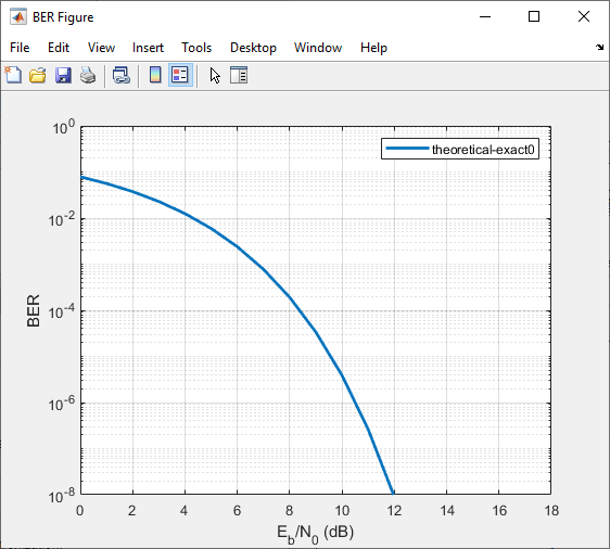
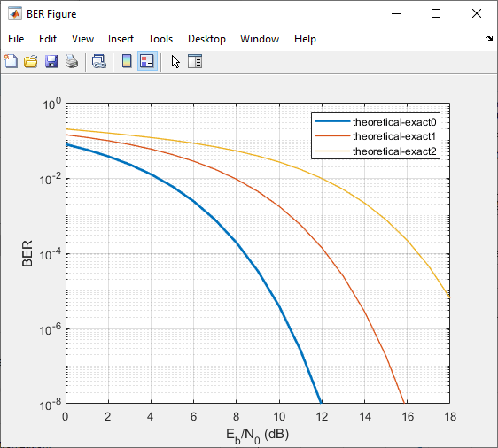
Available Sets of Theoretical BER Data
The Bit Error Rate Analysis app can generate a large set of
theoretical BERs. Parameters in the Theoretical tab enable
you to configure the channel type, modulation type and order, error detection
and correction channel coding, and synchronization error used when the app
computes the theoretical BER. The app adjusts the combination of selectable
parameter values based on your choices so that the configuration is always valid
or uses a dialog box to inform you of valid parameter values.
The app computes the theoretical BER for these modulation types, assuming Gray
ordered binary transmission data. The app uses these BER functions to perform
underlying computations and limits the modulation order to practical
limits.
-
berawgn— For AWGN
channel systems with no coding and perfect synchronization -
berfading— For
fading channel systems with no coding and perfect synchronization -
bercoding— For
systems with channel coding -
bersync— For
systems with BPSK modulation, no coding, and imperfect
synchronization -
berconfint—
For error probability estimate and confidence interval of Monte Carlo
simulation -
berfit— For
fitting curves to nonsmooth empirical BER data
To compute the BER for higher modulation orders than permitted in the app, use
the BER functions. For more information about specific combinations of
parameters, see the reference pages for the BER functions listed in the
Bit Error Rate Calculation and Estimation
function group of the Test and Measurement category.
Run MATLAB Simulations in Monte Carlo Tab
-
Section Overview
-
Use MATLAB Function with Bit Error Rate Analysis App
-
Assign Function Stopping Criteria
-
Plot Confidence Intervals
-
Curve Fit BER Points
Section Overview
Using the Monte Carlo tab with the Simulation
environment parameter set to MATLAB, you can
use the Bit Error Rate Analysis app in conjunction with your own
MATLAB communications system simulation functions to generate and analyze
BER data. The app calls the simulation specified by the Function
name parameter for each specified
Eb/N0
value, collects the BER data from the simulation, and creates a plot. The app
also enables you to adjust the
Eb/N0
range and the stopping criteria for the simulation.
To make your own simulation functions compatible with the app, see the Prepare MATLAB Function for Use in Bit Error Rate Analysis App example on the Bit Error Rate Analysis app reference
page.
Use MATLAB Function with Bit Error Rate Analysis App
This example shows how the Bit Error Rate Analysis app can run the
viterbisim
MATLAB simulation.
To run this example, follow these steps.
-
Open the Bit Error Rate Analysis app, and select the
Monte Carlo tab. -
Set these parameters to the specified values shown in this
table.Parameter Value Eb /
N0 range0:5Simulation
environmentMATLAB (default) Function name viterbisim(default)Number of Errors 100(default)Number of bits 1e8(default)
-
Click Run. The app runs the simulation function
once for each specified
Eb/N0
value and gathers BER data.Note
While the Bit Error Rate Analysis app runs the
configured simulation, it cannot process certain other tasks,
including plotting data from the other tabs of the user
interface. However, you can stop the simulation by clicking
Stop in the Monte Carlo Simulation
dialog box.After computing the BER for each of the specified
Eb/N0
values, the app creates a listing in the data viewer.The app also plots the data in the BER Figure window.

-
Adjust the
Eb/N0
range parameter to[5 5.2 5.3]and the
Number of bits parameter to
1e5. Click Run to produce
a new set of results.The app runs the simulation function using the new
Eb/N0
values and computes new BER data. The app then creates another listing
in the data viewer.
The app also plots the new data set in the BER Figure window,
adjusting the horizontal axis to accommodate the new
Eb/N0
values.The BER values for the 5 dB
Eb/N0
setting differ between the two sets of data because the number of bits
processed by the two simulations was different. If you want the computed
BER to converge to a stable value, set the number of bits high enough to
ensure that at least 100 bit errors occur. For more information about
the criteria used by the Bit Error Rate Analysis app to
terminate simulations, see the Assign Function Stopping Criteria section.
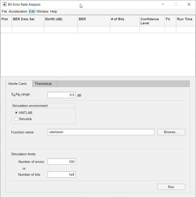
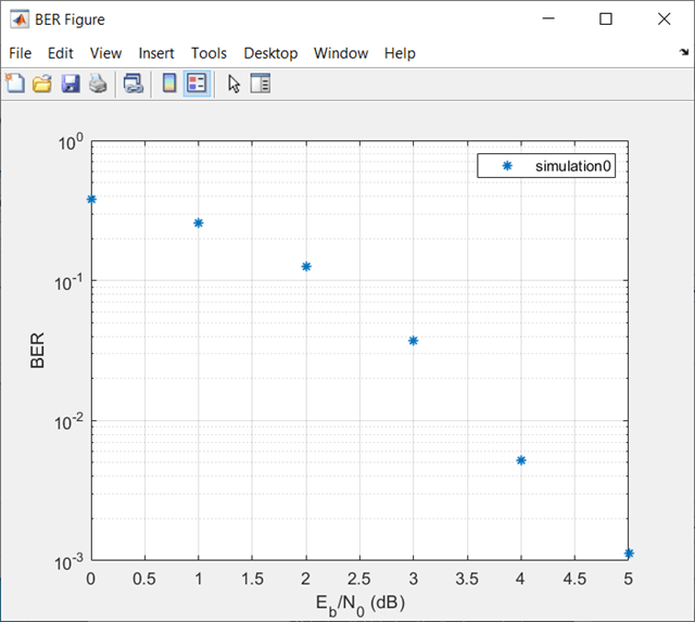
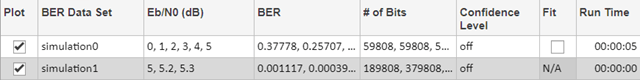

Assign Function Stopping Criteria
When you create a MATLAB simulation function for use with the Bit Error Rate
Analysis app, control the simulation run duration by setting the
target number of errors and maximum number of bits. The simulation stops the
current
Eb/N0
when either limit is reached. For more information about this requirement, see
the Requirements for Using MATLAB Functions with Bit Error Rate Analysis App section.
After you create your function, set the target number of errors and maximum
number of bits on the Monte Carlo tab of the app.
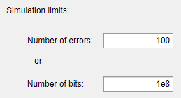
Typically, a Number of errors parameter value of at least
100 produces an accurate error rate. The Number
of bits value prevents the simulation from running too long.
Depending on the
Eb/N0
value and other aspects of the communications system modeled (such as modulation
characteristics and channel conditions), reaching 100 bit errors might not be
realistic. However, if fewer than 100 errors occur because the Number
of bits parameter value is too small, the returned error rate
might be misleading. You can use confidence intervals to gauge the accuracy of
the error rates that your simulation produces. As you increase the confidence
level, the accuracy of the computed error rate decreases.
As an example, follow the procedure described in the Use MATLAB Function with Bit Error Rate Analysis App section and set
the Confidence Level parameter value to
95 for each of the two data sets. The
confidence intervals for the second data set are larger than those for the
first data set because the BER values associated with the second data set
are based on only a small number of observed errors.
Note
As long as your function is set up to detect and react to the
Stop button in the Bit Error Rate
Analysis app, you can use the button to prematurely stop a series
of simulations. For more information, see Assign Function Stopping Criteria.
Plot Confidence Intervals
After you run a simulation with the Bit Error Rate Analysis app,
the resulting data set in the data viewer has an active menu in the
Confidence Level column. By default the
Confidence Level value is
off, meaning the simulation data in the BER
Figure window does not show confidence intervals.
To show confidence intervals in the BER Figure window, set
Confidence Level to 90%,
95%, or 99%.
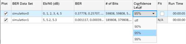
The plot in the BER Figure window automatically responds the
Confidence Level value change. This figure shows a
sample plot.
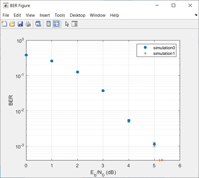
For an example that plots confidence intervals for a Simulink simulation, see the Use Simulink Model with Bit Error Rate Analysis App section.
To find confidence intervals for levels not listed in the Confidence
Level menu, use the berconfint function.
Curve Fit BER Points
After you run a simulation with the Bit Error Rate Analysis app,
the BER Figure window plots individual BER data points. To fit a curve to a data
set that contains at least four points, select Fit for that
data in the data viewer.

The plot in the BER Figure window automatically responds to this selection.
This plot shows a curve fit to a set of BER results.
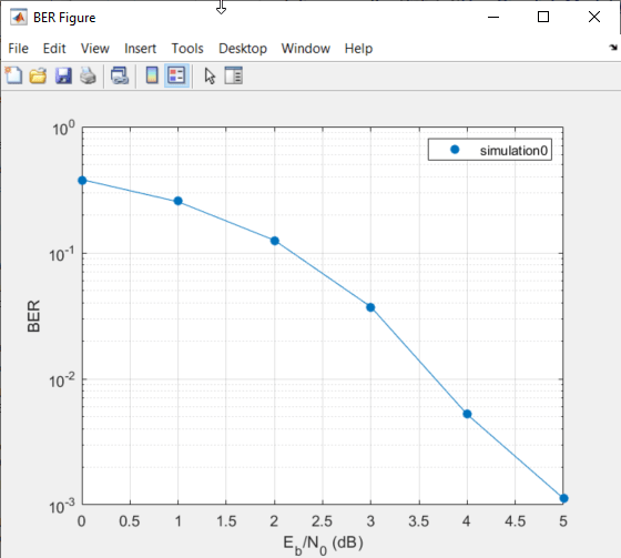
For greater flexibility in the process of fitting a curve to BER data, use the
berfit function.
Requirements for Using MATLAB Functions with Bit Error Rate Analysis App
When you create a MATLAB function for use with the Bit Error Rate Analysis app,
ensure the function interacts properly with the user interface. This section
describes the inputs, outputs, and basic operation of a function that is compatible
with the app.
Input Arguments
The Bit Error Rate Analysis app evaluates your entries in fields of the
user interface and passes data to the function as these input arguments (in
sequential order).
-
One value from the
Eb/N0
range vector each time the Bit Error Rate
Analysis app runs the simulation function -
Number of errors value
-
Number of bits value
Output Arguments
Your simulation function must compute and return these output arguments (in
sequential order). The Bit Error Rate Analysis app uses these output
arguments when reporting and plotting results.
-
Bit error rate of the simulation
-
Number of bits processed when computing the BER
Simulation Function Operation
Your simulation function must perform these tasks:
-
Simulate the communications system for the
Eb/N0
value specified in the first input argument. -
Stop simulating when the number of errors or number of processed bits
equals or exceeds the corresponding threshold specified in the second or
third input argument, respectively. -
Detect whether you click Stop in the Bit
Error Rate Analysis app to stop the simulation in that
case.
Template for Simulation Function
Use this template when adapting your code to work with the Bit Error Rate
Analysis app. You can open the template in an editor by entering
edit bertooltemplate at the MATLAB command prompt. If you develop a simulation function without using
the template, be sure your function satisfies the requirements described in the
Requirements for Using MATLAB Functions with Bit Error Rate Analysis App section.
function [ber,numBits] = bertooltemplateTemp(EbNo,maxNumErrs,maxNumBits,varargin)
%BERTOOLTEMPLATE Template for a BERTool (Bit Error Rate Analysis app) simulation function.
%   This file is a template for a BERTool-compatible simulation function.
%   To use the template, insert your own code in the places marked "INSERT
%   YOUR CODE HERE" and save the result as a file on your MATLAB path. Then
%   use the Monte Carlo pane of BERTool to execute the script.
%
%   [BER, NUMBITS] = YOURFUNCTION(EBNO, MAXNUMERRS, MAXNUMBITS) simulates
%   the error rate performance of a communications system. EBNO is a vector
%   of Eb/No values, MAXNUMERRS is the maximum number of errors to collect
%   before stopping the simulation, and MAXNUMBITS is the maximum number of
%   bits to run before stopping the simulation. BER is the computed bit error
%   rate, and NUMBITS is the actual number of bits run. Simulation can be
%   interrupted only after an Eb/No point is simulated.
%
%   [BER, NUMBITS] = YOURFUNCTION(EBNO, MAXNUMERRS, MAXNUMBITS, BERTOOL)
%   also provides BERTOOL, which is the handle for the BERTool app and can
%   be used to check the app status to interrupt the simulation of an Eb/No
%   point.
%
%   For more information about this template and an example that uses it,
%   see the Communications Toolbox documentation.
%
%   See also BERTOOL and VITERBISIM.

% Copyright 2020 The MathWorks, Inc.

% Initialize variables related to exit criteria.
totErr  = 0; % Number of errors observed
numBits = 0; % Number of bits processed

% --- Set up the simulation parameters. ---
% --- INSERT YOUR CODE HERE.

% Simulate until either the number of errors exceeds maxNumErrs
% or the number of bits processed exceeds maxNumBits.
while((totErr < maxNumErrs) && (numBits < maxNumBits))

    % Check if the user clicked the Stop button of BERTool.
    if isBERToolSimulationStopped(varargin{:})
      break
    end

    % --- Proceed with the simulation.
    % --- Be sure to update totErr and numBits.
    % --- INSERT YOUR CODE HERE.

end % End of loop

% Compute the BER.
ber = totErr/numBits;
About Template for Simulation Function
The simulation function template either satisfies the requirements listed in
the Requirements for Using MATLAB Functions with Bit Error Rate Analysis App section or indicates where you need to insert
code. In particular, the template:
-
Has appropriate input and output arguments
-
Includes a placeholder for code that simulates a system for the
given
Eb/N0
value -
Uses a loop structure to stop simulating when either the number of
errors exceedsmaxNumErrsor the number of bits
exceedsmaxNumBits, whichever occurs firstNote
Although the
whilestatement of the loop
describes the exit criteria, your own code inserted into the
section markedProceed with simulationmust
compute the number of errors and the number of bits. If you do
not perform these computations in your own code, clicking
Stop in the Monte Carlo Simulation
dialog box is the only way to terminate the loop. -
Detects when the user clicks Stop in the
Monte Carlo Simulation dialog box in each iteration of the
loop
Use Simulation Function Template
Follow these steps to update the simulation function template with your own
simulation code.
-
Place the code for setup tasks in the template section marked
Set up parameters. For example, initialize
variables such as those containing the modulation alphabet size,
filter coefficients, a convolutional coding trellis, or the states
of a convolutional interleaver. -
Place the code for these core simulation tasks in the template
section markedProceed with simulation. Determine
the core simulation tasks, assuming that all setup work has already
been performed. For example, core simulation tasks include
filtering, error-control coding, modulation and demodulation, and
channel modeling. -
Also in the template section marked
Proceed with, include code that updates the values of
simulation
thetotErrandnumBits
variables. ThetotErrvalue represents the number
of errors observed so far. ThenumBitsvalue
represents the number of bits processed so far. The computations to
update these variables depend on how your core simulation tasks
work.Note
Updating the numbers of errors and bits is important for
ensuring that the loop terminates. -
Omit from your simulation code any setup code that initializes
EbNo,maxNumErrs, or
maxNumBitsvariables, because the app passes
these quantities to the function as input arguments after evaluating
the data entered on the Monte Carlo tab. -
Adjust your code or the code of the template as necessary to use
consistent variable names and meanings. For example, if your
original code uses a variable calledebn0and the
function declaration (first line) for the template uses the variable
nameEbNo, you must change one of the names so
that they match. As another example, if your original code uses SNR
instead of
Eb/N0
values, you must convert values appropriately.
Compute Error Rate Simulation Sweeps Using Bit Error Rate Analysis App
Use the Bit Error Rate Analysis app to compute the BER as a function of Eb/N0. The app analyzes performance with either Monte Carlo simulations of MATLAB® functions and Simulink® models or theoretical closed-form expressions for selected types of communications systems. The code in the mpsksim.m function provides an M-PSK simulation that you can run from the Monte Carlo tab of the app.
Open the Bit Error Rate Analysis app from the Apps tab or by running the bertool function in the MATLAB command window.

On the Monte Carlo tab, set the Eb/N0 range parameter to 1:1:5 and the Function name parameter to mpsksim.
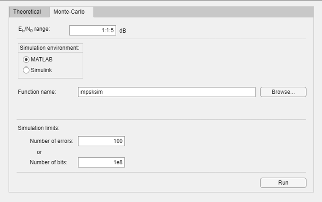
Open the mpsksim function for editing, set M=2, and save the changed file.
Run the mpsksim.m function as configured by clicking Run on the Monte Carlo tab in the app.
After the app simulates the set of Eb/N0 points, update the name of the BER data set results by selecting simulation0 in the BER Data Set field and typing M=2 to rename the set of results. The legend on the BER figure updates the label to M=2.


Update the value for M in the mpsksim function, repeating this process for M = 4, 8, and 16. For example, these figures of the Bit Error Rate Analysis app and BER Figure window show results for varying M values.
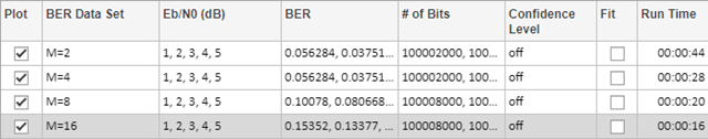

Parallel SNR Sweep Using Bit Error Rate Analysis App
The default configuration for the Monte Carlo processing of the Bit Error Rate Analysis app automatically uses parallel pool processing to process individual Eb/N0 points when you have the Parallel Computing Toolbox™ software but for the processing of your simulation code:
-
Any
parforfunction loops in your simulation code execute as standardforloops. -
Any
parfeval(Parallel Computing Toolbox) function calls in your simulation code execute serially. -
Any
spmd(Parallel Computing Toolbox) statement calls in your simulation code execute serially.

Copyright 2020 The MathWorks, Inc.
Run Simulink Simulations in Monte Carlo Tab
-
Section Overview
-
Use Simulink Model with Bit Error Rate Analysis App
-
Assign Model Stopping Criteria
Section Overview
You can use the Bit Error Rate Analysis app in conjunction with
Simulink models to generate and analyze BER data. The Simulink model simulates the performance of the communications system that
you want to study, while the Bit Error Rate Analysis app manages a
series of simulations using the model and collects the BER data.
Note
To use Simulink models within the Bit Error Rate Analysis app, you
must have the Simulink software.
To access the capabilities of the Bit Error Rate Analysis app
related to Simulink models, open the Monte Carlo tab, and then
set the Simulation environment parameter to
Simulink. If using parallel processing, the output must
be saved to a workspace variable so that the parallel running engine can collect
the results. For example, save the output of the Error Rate Calculation block to a
workspace variable by using a To Workspace (Simulink) block configured to
save the output to the name specified for the BER variable
name and with the Save format set to
Array.
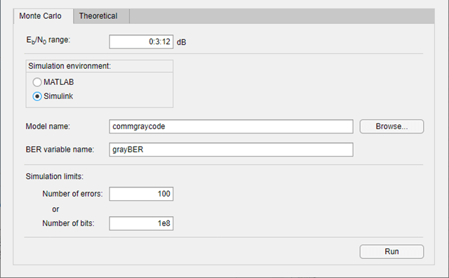
For details about confidence intervals and curve fitting for simulation data,
see the Plot Confidence Intervals and Curve Fit BER Points sections, respectively.
Use Simulink Model with Bit Error Rate Analysis App
This example shows how the Bit Error Rate Analysis app can manage a
series of simulations of a Simulink model and how you can vary the plot. This figure shows the
commgraycode model.
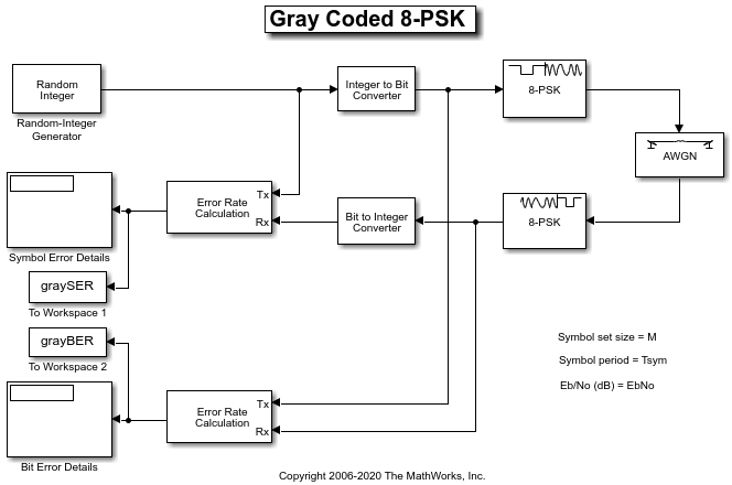
To run this example, follow these steps.
-
Open the Bit Error Rate Analysis app. On the
Monte Carlo tab, enter the Simulink model name and a BER variable name. The default value for
the Model name parameter is
commgraycode. the default value for the
BER variable name parameter is
grayBER. -
Click Run.
The Bit Error Rate Analysis app loads the model into
memory. The model initializes several variables in the MATLAB workspace. The app runs the simulation model once for each
Eb/N0
value, gathers the BER results, and creates a listing for the BER
results in the data viewer.
The Bit Error Rate Analysis app plots the data in the BER
Figure window. -
To fit a curve to the series of points in the BER Figure window,
select Fit for thesimulation0
data in the data viewer.The Bit Error Rate Analysis app plots the curve.
-
To indicate a 99% confidence interval around each point in the
simulation data, set Confidence Level to
99%in the data viewer.The Bit Error Rate Analysis app displays error bars to
represent the confidence intervals.

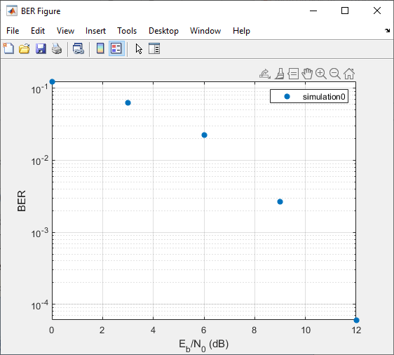
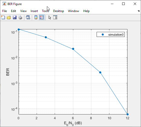
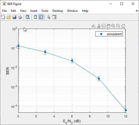
For another example that uses the Bit Error Rate Analysis app to
manage a series of Simulink simulations, see the Prepare Simulink Model for Use with Bit Error Rate Analysis App example on the Bit Error Rate Analysis app reference
page.
Assign Model Stopping Criteria
When you create a Simulink model for use with the Bit Error Rate Analysis app, you
must set it up so that the simulation ends when it either detects a target
number of errors or processes a maximum number of bits, whichever occurs first.
For more information about this requirement, see the Requirements for Using Simulink Models with Bit Error Rate Analysis App section.
After creating your Simulink model, set the target number of errors and the maximum number of
bits on the Monte Carlo tab of the Bit Error Rate
Analysis app.
Typically, a Number of errors parameter value of at least
100 produces an accurate error rate. The Number
of bits value prevents the simulation from running too long,
especially at large
Eb/N0
values. However, if the Number of bits value is so small
that the simulation collects very few errors, the error rate might not be
accurate. You can use confidence intervals to gauge the accuracy of the error
rates that your simulation produces. Larger confidence intervals result in less
accurate computed error rates.
You can also click Stop in the Monte Carlo Simulation
dialog box to stop a series of simulations prematurely.
Requirements for Using Simulink Models with Bit Error Rate Analysis App
When you create a Simulink model for use with the Bit Error Rate Analysis app, ensure
the model interacts properly with the user interface. This section describes the
inputs, outputs, and basic operation of a model that is compatible with the
app.
Input Variables
-
The channel block must use the
EbNovariable rather
than a hard-coded value for
Eb/N0.
For example, to model an AWGN channel, use the AWGN Channel block with the
Mode parameter set toSignal toand the Eb/No
noise ratio (Eb/No)
(dB) parameter set toEbNo. -
The simulation must stop either when the error count reaches the value
of themaxNumErrsvariable or when the number of
processed bits reaches the value of themaxNumBits
variable, whichever occurs first. You can configure the Error Rate Calculation block
in your model to use these criteria to stop the simulation.
Output Variables
-
The simulation must send the final error rate data to the MATLAB workspace as a variable whose name you enter in the
BER variable name parameter in the Bit
Error Rate Analysis app. The output error statistics variable
must be a three-element vector that lists the BER, the number of bit
errors, and the number of processed bits. -
The three-element vector format for the output error statistics is
supported by the Error Rate Calculation
block.
Simulation Model Operation
-
To avoid using an undefined variable name in blocks of the Simulink model, initialize these variables in the MATLAB workspace by using the preload callback function of the
model or by assigning them at the MATLAB command prompt.EbNo = 0; maxNumErrs = 100; maxNumBits = 1e8;
Tip
Using the preload function callback of the model to initialize the
runtime variables enables to you reopen the model in a future
MATLAB session with runtime variables preconfigured to run in
the app.The Bit Error Rate Analysis app provides the actual values
based on values in the Monte Carlo tab, so the
initial values in the model or workspace are not important. -
The app assumes the
Eb/N0
is used in the channel modeling. If your model uses the AWGN Channel block, and the
Mode parameter is not set to
Signal to noise ratio (Eb/No), adapt the
block to use the
Eb/N0
mode instead. For more information, see the AWGN Channel block reference
page. -
To compute the error rate, use the Error Rate Calculation block
with these parameter settings: select Stop
simulation, set Target number of
errors tomaxNumErrs, and set
Maximum number of symbols to
maxNumBits. -
If your model computes an SER instead of a BER, use the Integer to Bit Converter (Simulink)
block to convert symbols to bits. -
To send data from the Error Rate Calculation block
to the MATLAB workspace, set the Output data
parameter toPort, attach a To Workspace (Simulink) block to
the Error Rate Calculation block,
and set the Limit data points to last parameter of
the To Workspaceblock to1. The
Variable name parameter in the To
Workspace block must match the value you enter in the
BER variable name parameter of the Bit
Error Rate Analysis app. -
Frame-based simulations often run faster than sample-based simulations
for the same number of bits processed. With a frame-based simulation,
because the simulation processes a full frame of data each frame, the
number of errors or number of processed bits might exceed the values you
enter in the Bit Error Rate Analysis app. -
If your model uses a callback function to initialize variables in the
MATLAB workspace upon loading the model, before you click
Run in the Bit Error Rate Analysis
app, make sure that one of these conditions is met:-
The model is in memory (whether in a window or not), and the
variables are intact. -
The model is not currently in memory. In this case, the
Bit Error Rate Analysis app loads the model into
memory and runs the callback functions.
-
-
If you clear or overwrite the variables set in the model, clear the
model from memory by calling thebdclose(Simulink) function at
the MATLAB command prompt.When
you click Run in the Monte
Carlo tab, the app reloads the model.
Manage BER Data
-
Managing Data in Data Viewer
-
Export Bit Error Rate Analysis app Data Set
-
Save Bit Error Rate Analysis app Session
-
Import Bit Error Rate Analysis app Data Set
-
Open Previous Bit Error Rate Analysis app Session
Managing Data in Data Viewer
The data viewer gives you flexibility to rename and delete data sets and to
reorder columns in the data viewer.
-
To rename a data set in the data viewer, double-click its name in the
BER Data Set column and type a new name.
-
To delete a data set from the data viewer, select the data set, then
select .Note
If the data set originated from the
Theoretical tab, the Bit Error Rate
Analysis app deletes the data without asking for
confirmation. You cannot undo this operation.
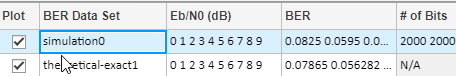
Export Bit Error Rate Analysis app Data Set
The Bit Error Rate Analysis app enables you to export individual
data sets to the MATLAB workspace or to MAT-files. Exporting data enables you to process
the data outside the Bit Error Rate Analysis app. For example, to
create customized plots using data from the Bit Error Rate Analysis
app, export the app data set to the MATLAB workspace and use any of the plotting commands in MATLAB. To reimport a structure later, see the Import Bit Error Rate Analysis app Data Set section.
To export an individual data set, follow these steps.
-
In the data viewer, select the data set you want to export.
-
Select . Set
Export to to indicate the format and
destination of the data.-
Workspace arrays— Export
the selected data set to a pair of arrays in the
MATLAB workspace. Use this option if you want to
access the data in the MATLAB workspace (outside the app) and if you do
not need to import the data into the Bit Error Rate
Analysis app later.Under Variable names, set
Eb/N0
and BER parameters to specify the
variable names for the
Eb/N0
values and BER values, respectively.
If you want the Bit Error Rate Analysis app
to use your chosen variable names even if variables by
those names already exist in the workspace, select
Overwrite variables. -
Workspace structure—
Export the selected data set to a structure in the
MATLAB workspace. If you export data using this
option, you can import the data structure into the
Bit Error Rate Analysis app later.Set the Structure name parameter
to specify a workspace structure name.If you want the Bit Error Rate Analysis app
to use your chosen variable name even if a variable with
that name already exist in the workspace, select
Overwrite variables. -
MAT-file— Export the
selected data set to a structure in a MAT-file. If you
export data using this option, you can import a MAT-file
data structure into the Bit Error Rate
Analysis app later.Set the Structure name in file
parameter to specify a MAT-file name. The structure name
in the file will also use this name.
-
-
Click OK. If you set Export
to toMAT-file, the
Bit Error Rate Analysis app prompts you for the path
to the MAT-file that you want to create.
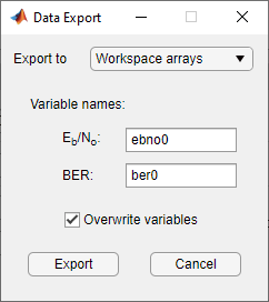
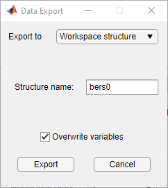
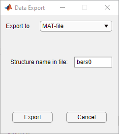
Examine an Exported Structure
This section describes the contents of the structure that the Bit Error
Rate Analysis app exports to the workspace or to a MAT-file. This
table describes the fields of the exported data structure. When you want to
manipulate exported data, the fields that are most relevant are
paramsEvaled and data.
| Field | Description |
|---|---|
params |
The parameter values in the Bit Error Rate Analysis app, some of which might be invisible and hence irrelevant for computations |
paramsEvaled |
The parameter values evaluated and used by the Bit Error Rate Analysis app when computing the data set |
data |
The Eb/N0, BER, and number of bits processed |
dataView |
Information about the appearance in the data viewer, which is used by the Bit Error Rate Analysis app when reimporting the data |
cellEditabilities |
Indication whether the data viewer has an active Confidence Level or Fit entry, which is used by the Bit Error Rate Analysis app when reimporting the data |
Parameter Fields
The params and paramsEvaled fields are
similar to each other, except that params describes the exact
state of the user interface, whereas paramsEvaled indicates
the values that are actually used for computations. For example, in a
theoretical system with an AWGN channel, params records but
paramsEvaled omits a diversity order parameter. The
diversity order is not used in the computations because it is relevant for only
systems with Rayleigh channels. As another example, if you type
[0:3]+1 in the user interface as the range of
Eb/N0
values, params indicates [0:3]+1, whereas
paramsEvaled indicates 1 2 3 4.
The length and exact contents of paramsEvaled depend on the
data set because only relevant information appears. If the meaning of the
contents of paramsEvaled is not clear upon inspection, one
way to learn more is to reimport the data set into the Bit Error Rate
Analysis app and inspect the parameter values that appear in the user
interface.
Data Field
If your exported workspace variable is called ber0, the
field ber0.data is a cell array that contains the numerical
results in these vectors:
-
ber0.data{1}lists the
Eb/N0
values. -
ber0.data{2}lists the BER values corresponding to
each of the
Eb/N0
values. -
ber0.data{3}indicates, for simulation results, how
many bits the Bit Error Rate Analysis app processed when
computing each of the corresponding BER values.
Save Bit Error Rate Analysis app Session
The Bit Error Rate Analysis app enables you to save an entire
session. This feature is useful if your session contains multiple data sets that
you want to return to in a later session. To reimport a saved session, see the
Open Previous Bit Error Rate Analysis app Session
section.
To save an entire Bit Error Rate Analysis app session, follow these steps.
-
Select .
-
When the Bit Error Rate Analysis app prompts you, enter
the path to the file that you want to create.
The Bit Error Rate Analysis app saves the data in a MAT file or a
binary file that records all data sets currently in the data viewer along with
the user interface parameters associated with the data sets.
Note
If your Bit Error Rate Analysis app session requires particular
workspace variables, save those separately in a MAT-file using the
save command in MATLAB.
Import Bit Error Rate Analysis app Data Set
The Bit Error Rate Analysis app enables you to reimport individual
data sets that you previously exported to a structure. For more information
about exporting data sets from the Bit Error Rate Analysis app, see
the Export Bit Error Rate Analysis app Data Set section.
To import an individual data set that you previously exported from the
Bit Error Rate Analysis app to a structure, follow these steps.
-
Select .

-
Set the Import from parameter to either
Workspace structureor
MAT-file. If you select
Workspace structure, type the name of
the workspace variable in the Structure name
parameter. -
Click OK. If you set Import
from toMAT-file, the
Bit Error Rate Analysis app prompts you to select the
file that contains the structure you want to import.
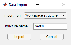
After you dismiss the Data Import dialog box (and the file selection dialog
box, in the case of a MAT-file), the data viewer shows the newly imported data
set and the BER Figure window the corresponding plot.
Open Previous Bit Error Rate Analysis app Session
The Bit Error Rate Analysis app enables you to open previous saved
sessions. For more information about exporting data sets from the Bit Error
Rate Analysis app, see the Save Bit Error Rate Analysis app Session section.
To replace the data sets in the data viewer with data sets from a previous
Bit Error Rate Analysis app session, follow these steps.
-
Select .
Note
If the Bit Error Rate Analysis app already contains
data sets, your are asked whether you want to save the current
session. If you answer no and continue with the loading process,
the Bit Error Rate Analysis app discards the current
session upon opening a new session from the file. -
When the Bit Error Rate Analysis app prompts you, enter
the path to the file you want to open. It must be a file that you
previously created using the
option in the Bit Error Rate Analysis app.
After the Bit Error Rate Analysis app reads the session file, the
data viewer shows the data sets from the file.
If the Bit Error Rate Analysis app session requires particular
workspace variables that you saved separately in a MAT-file, you can retrieve
them by using the load function at the
MATLAB command prompt. For example, to load the Bit Error Rate
Analysis app session named
ber_analysis_filename.mat enter this command.
load ber_analysis_filename.mat
See Also
Apps
- Bit Error Rate Analysis
Functions
berawgn|bercoding|berconfint|berfading|berfit|bersync
Related Topics
- Bit Error Rate Analysis Techniques
- Analytical Expressions Used in BER Analysis
You might be a communication system designer, or a newbie in communication. While designing or applying any of the modulation scheme with or without modulation for any type of channel you need to have the information of the Bit Error Rate for a particular SNR, so that you can decide on the various parameters of your system (for e.g., transmit power). Or sometime you just want to compare your developed system or scheme with the currently available theoretical references of the BER values. For that need MATLAB’s communication system toolbox has been bundled with a tool, in which you just need to select a few options & there you will get the result you want for the BERs.
So assuming you did already installed MATLAB’s Communication System Toolbox, for starting the Bit Error Analysis Tool you just need to type & enter the command in the MATLAB’s command window as «bertool«.
That will popup a window like this,
 |
| The Bit Error Analysis Tool in MATLAB’s Communication System Toolbox: BERTOOL |
The file menu has some options for the user.

That is, New Session, Open Session, Save Session, Import Data & Export Data. The Export Data, will be enabled when you have already did a simulation, which you can later on import, through, Import Data option.
In the tabs below, the Theoretical Tab, you may be seeing various options, one of them is the Eb/No range setting.
 |
| Eb/No Range Set in BERTOOL: Bit Error Analysis Tool in MATLAB Communication System Toolbox |
If you want it to be in the range -6 to 20 dB you just need to specify it as, -6:20 in the above input box. This will serve as your x-axis while the BER plot has been generated.
Below that, there is also an option to select the channel type, it provides us with three options,
AWGN, Rayleigh, & Rician. After the selection you will get various other options related to these channel that you can tweak in to further control your channel.
 |
| Channel Type AWGN in BERTOOL : Bit Error Analysis Tool in MATLAB Communication System Toolbox |
 |
| Channel Type Rayleigh in BERTOOL : Bit Error Analysis Tool in MATLAB Communication System Toolbox |
 |
| Channel Type Rician in BERTOOL : Bit Error Analysis Tool in MATLAB Communication System Toolbox |
It provides Various options in Modulation Schemes even.
Namely, PSK, DPSK, OQPSK, PAM, QAM, FSK, MSK, & CPFSK.
 |
| Modulation Type in BERTOOL: Bit Error Analysis Tool in MATLAB Communication System Toolbox |
 |
| Selection of Modulation Order, in BERTOOL |
So, for a M-Ary modulation scene you got various options, i.e., from 2 to 64.
Select & browse through various modulation schemes & you will be seeing various options enabling & disabling with them.
Like while selecting the PSK & OQPSK, you will see an option to enable Differential Encoding to appear & demodulation type option is disabled. And while selecting PAM, QAM, FSK you will not see any option of Differential Encoding.
Like wise you need to select what your communication system requires.
For Channel Coding part, You need to select Either, None, Convolutional or Block type of Coding.
While selecting the Convolutional coding, you need to specify the trellis polynomial & what decision method you will use while decoding it.
 |
| Channel Coding Methods in MATLAB «bertool» : Bit Error Analysis Tool in MATLAB Communication System Toolbox |
Another coding type will be the Block Code. Below are the various options available with it.
 |
| Block Coding Option in MATLAB «bertool» : Bit Error Analysis Tool in MATLAB Communication System Toolbox |
At last to generate a MATLAB BER vs SNR plot just press the button, «Plot».
I have selected, to plot from 0 to 18 dB SNR, AWGN Channel. 4-QAM modulation, with convolutional code, hard decision & the Trellis polynomial is represented by, poly2trellis(7, [171 133]). The result is,
 |
| BER Plot, MATLAB 4-QAM, AWGN Channel, With Convolutional Coding/Decoding. |
So when you run a simulation you get to see something new at the top, which is the data associated with the simulation that you can save, & reload for the next time if you want.
 |
| The data after the simulation has completed. MATLAB bertool. |
The semianalytic mode of MATLAB BERtool, has the same functionality, but it gives more flexibility in terms of deciding the bits/symbols to get an analysis of. And additionally the receiver filter coefficient has been added.
 |
| The Semianalytic Mode for the BERTOOL MATLAB. |
You at last can do, Monte Carlo simulation also in MATLAB’s BERTOOL. With various options.
 |
| Option of Monte Carlo Simulation in bertool, in MATLAB |
So, have a happy day with the BERTOOL of MATLAB. I am sure that this tool will be handy for you, if you need a serious wireless system design.

An active & prominent author at Digital iVision Labs! Specializing in MATLAB, C++, Arduino, OpenCV, NI Labview, Web Designing & other Electronics stuffs! Just started M.Tech. From IIIT Delhi, looking for excellent PhD Opportunities with prominent researchers. Drop a mail: vibhutesh[at]gmail.com or Follow him at….
This is machine translation
Translated by ![]()
Mouseover text to see original. Click the button below to return to the English version of the page.
Note: This page has been translated by MathWorks. Click here to see
To view all translated materials including this page, select Country from the country navigator on the bottom of this page.
Theoretical Results
Common Notation
The following notation is used throughout this Appendix:
| Quantity or Operation | Notation |
|---|---|
| Size of modulation constellation |
M |
| Number of bits per symbol |
k=log2M |
| Energy per bit-to-noise power-spectral-density ratio |
EbN0 |
| Energy per symbol-to-noise power-spectral-density ratio |
EsN0=kEbN0 |
| Bit error rate (BER) |
Pb |
| Symbol error rate (SER) |
Ps |
| Real part |
Re[⋅] |
| Largest integer smaller than |
⌊⋅⌋ |
The following mathematical functions are used:
| Function | Mathematical Expression |
|---|---|
| Q function |
Q(x)=12π∫x∞exp(−t2/2)dt |
| Marcum Q function |
Q(a,b)=∫b∞texp(−t2+a22)I0(at)dt |
| Modified Bessel function of the first kind of order ν |
Iν(z)=∑k=0∞(z/2)υ+2kk!Γ(ν+k+1) where Γ(x)=∫0∞e−ttx−1dt is the gamma function. |
| Confluent hypergeometric function |
F11(a,c;x)=∑k=0∞(a)k(c)kxkk! where the Pochhammer symbol, (λ)k, is defined as (λ)0=1, (λ)k=λ(λ+1)(λ+2)⋯(λ+k−1). |
The following acronyms are used:
| Acronym | Definition |
|---|---|
| M-PSK | M-ary phase-shift keying |
| DE-M-PSK | Differentially encoded M-ary phase-shift keying |
| BPSK | Binary phase-shift keying |
| DE-BPSK | Differentially encoded binary phase-shift keying |
| QPSK | Quaternary phase-shift keying |
| DE-QPSK | Differentially encoded quadrature phase-shift keying |
| OQPSK | Offset quadrature phase-shift keying |
| DE-OQPSK | Differentially encoded offset quadrature phase-shift keying |
| M-DPSK | M-ary differential phase-shift keying |
| M-PAM | M-ary pulse amplitude modulation |
| M-QAM | M-ary quadrature amplitude modulation |
| M-FSK | M-ary frequency-shift keying |
| MSK | Minimum shift keying |
| M-CPFSK | M-ary continuous-phase frequency-shift keying |
Analytical Expressions Used in berawgn
-
M-PSK
-
DE-M-PSK
-
OQPSK
-
DE-OQPSK
-
M-DPSK
-
M-PAM
-
M-QAM
-
Orthogonal M-FSK with Coherent Detection
-
Nonorthogonal 2-FSK with Coherent Detection
-
Orthogonal M-FSK with Noncoherent Detection
-
Nonorthogonal 2-FSK with Noncoherent Detection
-
Precoded MSK with Coherent Detection
-
Differentially Encoded MSK with Coherent Detection
-
MSK with Noncoherent Detection (Optimum Block-by-Block)
-
CPFSK Coherent Detection (Optimum Block-by-Block)
M-PSK. From equation 8.22 in [2]
The following expression is very close, but not strictly equal,
to the exact BER (from [4] and equation 8.29 from [2]):
where wi’=wi+wM−i, wM/2’=wM/2, wiis the Hamming weight of bits
assigned to symbol i, and
Special case of M=2, e.g., BPSK (equation
5.2-57 from [1]):
Special case of M=4, e.g., QPSK (equations
5.2-59 and 5.2-62 from [1]):
DE-M-PSK. M=2, e.g., DE-BPSK (equation 8.36
from [2]):
M=4, e.g., DE-QPSK (equation 8.38
from [2]):
From equation 5 in [3]:
OQPSK. Same BER/SER as QPSK [2].
DE-OQPSK. Same BER/SER as DE-QPSK [3].
M-DPSK. From equation 8.84 in [2]:
The following expression is very close, but not strictly equal,
to the exact BER [4]:
where wi’=wi+wM−i, wM/2’=wM/2, wi is the Hamming weight of bits
assigned to symbol i, and
Special case of M=2 (equation 8.85
from [2]):
M-PAM. From equations 8.3 and 8.7 in [2], and
equation 5.2-46 in [1]:
From [5]:
M-QAM. For square M-QAM, k=log2M is even (equation
8.10 from [2], and
equations 5.2-78 and 5.2-79 from [1]):
From [5]:
For rectangular (non-square) M-QAM, k=log2M is odd, M=I×J, I=2k−12, and J=2k+12:
From [5]:
where
and
Orthogonal M-FSK with Coherent Detection. From equation 8.40 in [2] and
equation 5.2-21 in [1]:
Nonorthogonal 2-FSK with Coherent Detection. For M=2 (from equation 5.2-21 in [1] and equation 8.44 in [2]):
ρis the complex correlation coefficient:
where s˜1(t) and s˜2(t) are complex lowpass signals,
and
For example:
where Δf=f1−f2.
(from equation 8.44 in [2], where h=ΔfTb)
Orthogonal M-FSK with Noncoherent Detection. From equation 5.4-46 in [1] and equation 8.66 in [2]:
Nonorthogonal 2-FSK with Noncoherent Detection. For M=2 (from equation 5.4-53 in [1] and equation 8.69 in [2]):
where
Precoded MSK with Coherent Detection. Same BER/SER as BPSK.
Differentially Encoded MSK with Coherent Detection. Same BER/SER as DE-BPSK.
MSK with Noncoherent Detection (Optimum Block-by-Block). Upper bound (from equations 10.166 and 10.164 in [6]):
where
CPFSK Coherent Detection (Optimum Block-by-Block). Lower bound (from equation 5.3-17 in [1]):
Upper bound:
where h is the modulation index, and Kδmin is the number of paths having
the minimum distance.
Analytical Expressions Used in berfading
-
Notation
-
M-PSK with MRC
-
DE-M-PSK with MRC
-
M-PAM with MRC
-
M-QAM with MRC
-
M-DPSK with Postdetection EGC
-
Orthogonal 2-FSK, Coherent Detection with MRC
-
Nonorthogonal 2-FSK, Coherent Detection with MRC
-
Orthogonal M-FSK, Noncoherent Detection with EGC
-
Nonorthogonal 2-FSK, Noncoherent Detection with No Diversity
Notation. The following notation is used for the expressions found in berfading.
| Value | Notation |
|---|---|
| Power of the fading amplitude r | Ω=E[r2], where E[⋅] denotes statistical expectation |
| Number of diversity branches |
L |
| SNR per symbol per branch |
γ¯l=(ΩlEsN0)/L=(ΩlkEbN0)/L For identically-distributed diversity γ¯=(ΩkEbN0)/L |
| Moment generating functions for each diversity branch |
Rayleigh fading: Mγl(s)=11−sγ¯l Rician fading: Mγl(s)=1+K1+K−sγ¯le[Ksγ¯l(1+K)−sγ¯l] where K is the ratio of For |
The following acronyms are used:
| Acronym | Definition |
|---|---|
| MRC | maximal-ratio combining |
| EGC | equal-gain combining |
M-PSK with MRC. From equation 9.15 in [2]:
From [4] and [2]:
where wi’=wi+wM−i, wM/2’=wM/2, wi is the Hamming weight of bits
assigned to symbol i, and
For the special case of Rayleigh fading with M=2 (from equations C-18, C-21,
and Table C-1 in [6]):
where
If L=1:
DE-M-PSK with MRC. For M=2 (from equations 8.37 and 9.8-9.11
in [2]):
M-PAM with MRC. From equation 9.19 in [2]:
From [5] and [2]:
M-QAM with MRC. For square M-QAM, k=log2M is even (equation
9.21 in [2]):
From [5] and [2]:
For rectangular (nonsquare) M-QAM, k=log2M is odd, M=I×J, I=2k−12, J=2k+12, γ¯l=Ωllog2(IJ)EbN0, and
From [5] and [2]:
M-DPSK with Postdetection EGC. From equation 8.165 in [2]:
From [4] and [2]:
where wi’=wi+wM−i, wM/2’=wM/2, wi is the Hamming weight of bits
assigned to symbol i, and
For the special case of Rayleigh fading with M=2, and L=1 (equation 8.173 from [2]):
Orthogonal 2-FSK, Coherent Detection with MRC. From equation 9.11 in [2]:
For the special case of Rayleigh fading (equations 14.4-15 and
14.4-21 in [1]):
Nonorthogonal 2-FSK, Coherent Detection with MRC. Equations 9.11 and 8.44 in [2]:
For the special case of Rayleigh fading with L=1 (equation 20 in [8] and equation 8.130 in [2]):
Orthogonal M-FSK, Noncoherent Detection with EGC. Rayleigh fading (equation 14.4-47 in [1]):
Rician fading (equation 41 in [8]):
where
and I[a,b](i)=1 if a≤i≤b and 0 otherwise.
Nonorthogonal 2-FSK, Noncoherent Detection with No Diversity. From equation 8.163 in [2]:
where
Analytical Expressions Used in bercoding and BERTool
-
Common Notation for This Section
-
Block Coding
-
Convolutional Coding
Common Notation for This Section
| Description | Notation |
|---|---|
| Energy-per-information bit-to-noise power-spectral-density ratio |
γb=EbN0 |
| Message length |
K |
| Code length |
N |
| Code rate |
Rc=KN |
Block Coding. Specific notation for block coding expressions: dmin is the minimum distance of the
code.
Soft Decision
BPSK, QPSK, OQPSK, PAM-2, QAM-4, and precoded MSK (equation 8.1-52 in
[1]):
DE-BPSK, DE-QPSK, DE-OQPSK, and DE-MSK:
BFSK, coherent detection (equations 8.1-50 and 8.1-58 in [1]):
BFSK, noncoherent square-law detection (equations 8.1-65 and 8.1-64 in
[1]):
DPSK:
Hard Decision
General linear block code (equations 4.3, 4.4 in [9], and 12.136 in [6]):
Hamming code (equations 4.11, 4.12 in [9], and 6.72, 6.73 in [7]):
(24, 12) extended Golay code (equation 4.17 in [9], and 12.139 in [6]):
where βm is the average number of channel symbol errors that remain
in corrected N-tuple when the channel caused
m symbol errors (table 4.2 in [9]).
Reed-Solomon code with N=Q−1=2q−1:
for FSK (equations 4.25, 4.27 in [9], 8.1-115, 8.1-116 in [1], 8.7, 8.8 in [7], and 12.142, 12.143 in [6]), and
otherwise.
If log2Q/log2M=q/k=h where h is an integer (equation 1 in
[10]):
where s is the symbol error rate (SER) in an uncoded
AWGN channel.
For example, for BPSK, M=2 and Ps=1−(1−s)q
Otherwise, Ps is given by table 1 and equation 2 in [10].
Convolutional Coding. Specific notation for convolutional coding expressions: dfree is the free distance of the
code, and ad is the number of paths of distance d from
the all-zero path that merge with the all-zero path for the first
time.
Soft Decision
From equations 8.2-26, 8.2-24, and 8.2-25 in [1], and equations 13.28 and 13.27 in [6]:
with transfer function
where f(d) is the exponent of N as a function of
d.
Results for BPSK, QPSK, OQPSK, PAM-2, QAM-4, precoded MSK, DE-BPSK,
DE-QPSK, DE-OQPSK, DE-MSK, DPSK, and BFSK are obtained as:
where Pb is the BER in the corresponding uncoded AWGN channel. For
example, for BPSK (equation 8.2-20 in [1]):
Hard Decision
From equations 8.2-33, 8.2-28, and 8.2-29 in [1], and equations 13.28, 13.24, and 13.25 in [6]:
where
when d is odd, and
when d is even (p is the bit error
rate (BER) in an uncoded AWGN channel).
Performance Results via Simulation
-
Section Overview
-
Using Simulated Data to Compute Bit and Symbol Error Rates
-
Example: Computing Error Rates
-
Comparing Symbol Error Rate and Bit Error Rate
Section Overview
One way to compute the bit error rate or symbol error rate for a communication system is to
simulate the transmission of data messages and compare all messages before and
after transmission. The simulation of the communication system components using
Communications Toolbox™ is covered in other parts of this guide. This section describes
how to compare the data messages that enter and leave the simulation.
Another example of computing performance results via simulation
is in Curve Fitting for Error Rate Plots in the discussion of curve
fitting.
Using Simulated Data to Compute Bit and Symbol Error Rates
The biterr function compares two sets of
data and computes the number of bit errors and the bit error rate.
The symerr function compares two sets of data
and computes the number of symbol errors and the symbol error rate.
An error is a discrepancy between corresponding points in the two
sets of data.
Of the two sets of data, typically one represents messages entering
a transmitter and the other represents recovered messages leaving
a receiver. You might also compare data entering and leaving other
parts of your communication system, for example, data entering an
encoder and data leaving a decoder.
If your communication system uses several bits to represent
one symbol, counting bit errors is different from counting symbol
errors. In either the bit- or symbol-counting case, the error rate
is the number of errors divided by the total number (of bits or symbols)
transmitted.
Note
To ensure an accurate error rate, you should typically simulate
enough data to produce at least 100 errors.
If the error rate is very small (for example, 10-6 or
smaller), the semianalytic technique might compute the result more
quickly than a simulation-only approach. See Performance Results via the Semianalytic Technique for more
information on how to use this technique.
Example: Computing Error Rates
The script below uses the symerr function
to compute the symbol error rates for a noisy linear block code. After
artificially adding noise to the encoded message, it compares the
resulting noisy code to the original code. Then it decodes and compares
the decoded message to the original one.
m = 3; n = 2^m-1; k = n-m; % Prepare to use Hamming code.
msg = randi([0 1],k*200,1); % 200 messages of k bits each
code = encode(msg,n,k,'hamming');
codenoisy = rem(code+(rand(n*200,1)>.95),2); % Add noise.
% Decode and correct some errors.
newmsg = decode(codenoisy,n,k,'hamming');
% Compute and display symbol error rates.
noisyVec = step(comm.ErrorRate,code,codenoisy);
decodedVec = step(comm.ErrorRate,msg,newmsg);
disp(['Error rate in the received code: ',num2str(noisyVec(1))])
disp(['Error rate after decoding: ',num2str(decodedVec(1))])
The output is below. The error rate decreases after decoding
because the Hamming decoder corrects some of the errors. Your results
might vary because this example uses random numbers.
Error rate in the received code: 0.054286
Error rate after decoding: 0.03
Comparing Symbol Error Rate and Bit Error Rate
In the example above, the symbol errors and bit errors are the
same because each symbol is a bit. The commands below illustrate the
difference between symbol errors and bit errors in other situations.
a = [1 2 3]'; b = [1 4 4]';
format rat % Display fractions instead of decimals.
% Create ErrorRate Calculator System object
serVec = step(comm.ErrorRate,a,b);
srate = serVec(1)
snum = serVec(2)
% Convert integers to bits
hIntToBit = comm.IntegerToBit(3);
a_bit = step(hIntToBit, a);
b_bit = step(hIntToBit, b);
% Calculate BER
berVec = step(comm.ErrorRate,a_bit,b_bit);
brate = berVec(1)
bnum = berVec(2)
The output is below.
snum =

      2


srate =

     2/3


bnum =

      5


brate =

     5/9
bnum is 5 because the second entries differ
in two bits and the third entries differ in three bits. brate is
5/9 because the total number of bits is 9. The total number of bits
is, by definition, the number of entries in a or b times
the maximum number of bits among all entries of a and b.
Performance Results via the Semianalytic Technique
The technique described in Performance Results via Simulation works well for a large
variety of communication systems, but can be prohibitively time-consuming
if the system’s error rate is very small (for example, 10-6 or
smaller). This section describes how to use the semianalytic technique
as an alternative way to compute error rates. For certain types of
systems, the semianalytic technique can produce results much more
quickly than a nonanalytic method that uses only simulated data.
The semianalytic technique uses a combination of simulation
and analysis to determine the error rate of a communication system.
The semianalytic function in Communications Toolbox helps
you implement the semianalytic technique by performing some of the
analysis.
When to Use the Semianalytic Technique
The semianalytic technique works well for certain types of communication
systems, but not for others. The semianalytic technique is applicable
if a system has all of these characteristics:
-
Any effects of multipath fading, quantization, and
amplifier nonlinearities must precede the effects
of noise in the actual channel being modeled. -
The receiver is perfectly synchronized with the carrier,
and timing jitter is negligible. Because phase noise and timing jitter
are slow processes, they reduce the applicability of the semianalytic
technique to a communication system. -
The noiseless simulation has no errors in the received
signal constellation. Distortions from sources other than noise should
be mild enough to keep each signal point in its correct decision region.
If this is not the case, the calculated BER is too low. For instance,
if the modeled system has a phase rotation that places the received
signal points outside their proper decision regions, the semianalytic
technique is not suitable to predict system performance.
Furthermore, the semianalytic function
assumes that the noise in the actual channel being modeled is Gaussian.
For details on how to adapt the semianalytic technique for non-Gaussian
noise, see the discussion of generalized exponential distributions
in [11].
Procedure for the Semianalytic Technique
The procedure below describes how you would typically implement
the semianalytic technique using the semianalytic function:
-
Generate a message signal containing at least ML symbols,
where M is the alphabet size of the modulation and L is the length
of the impulse response of the channel in symbols. A common approach
is to start with an augmented binary pseudonoise (PN) sequence of
total length(log2M)ML.
An augmented PN sequence is a PN sequence with
an extra zero appended, which makes the distribution of ones and zeros
equal. -
Modulate a carrier with the message signal using baseband modulation.
Supported modulation types are listed on the reference page forsemianalytic.
Shape the resultant signal with rectangular pulse shaping, using
the oversampling factor that you will later use to filter the modulated
signal. Store the result of this step astxsigfor
later use. -
Filter the modulated signal with a transmit filter. This filter
is often a square-root raised cosine filter, but you can also use
a Butterworth, Bessel, Chebyshev type 1 or 2, elliptic, or more general
FIR or IIR filter. If you use a square-root raised cosine filter,
use it on the nonoversampled modulated signal and specify the oversampling
factor in the filtering function. If you use another filter type,
you can apply it to the rectangularly pulse shaped signal. -
Run the filtered signal through a noiseless channel.
This channel can include multipath fading effects, phase shifts,
amplifier nonlinearities, quantization, and additional filtering,
but it must not include noise. Store the result of this step asrxsigfor
later use. -
Invoke the
semianalyticfunction
using thetxsigandrxsigdata
from earlier steps. Specify a receive filter as a pair of input arguments,
unless you want to use the function’s default filter. The function
filtersrxsigand then determines the error probability
of each received signal point by analytically applying the Gaussian
noise distribution to each point. The function averages the error
probabilities over the entire received signal to determine the overall
error probability. If the error probability calculated in this way
is a symbol error probability, the function converts it to a bit error
rate, typically by assuming Gray coding. The function returns the
bit error rate (or, in the case of DQPSK modulation, an upper bound
on the bit error rate).
Example: Using the Semianalytic Technique
The example below illustrates the procedure described above,
using 16-QAM modulation. It also compares the error rates obtained
from the semianalytic technique with the theoretical error rates obtained
from published formulas and computed using the berawgn function.
The resulting plot shows that the error rates obtained using the two
methods are nearly identical. The discrepancies between the theoretical
and computed error rates are largely due to the phase offset in this
example’s channel model.
% Step 1. Generate message signal of length >= M^L.
M = 16; % Alphabet size of modulation
L = 1; % Length of impulse response of channel
msg = [0:M-1 0]; % M-ary message sequence of length > M^L

% Step 2. Modulate the message signal using baseband modulation.
%hMod = comm.RectangularQAMModulator(M);  % Use 16-QAM.
%modsig = step(hMod,msg'); % Modulate data
modsig = qammod(msg',M); % Modulate data
Nsamp = 16;
modsig = rectpulse(modsig,Nsamp); % Use rectangular pulse shaping.

% Step 3. Apply a transmit filter.
txsig = modsig; % No filter in this example

% Step 4. Run txsig through a noiseless channel.
rxsig = txsig*exp(1i*pi/180); % Static phase offset of 1 degree
% Step 5. Use the semianalytic function.
% Specify the receive filter as a pair of input arguments.
% In this case, num and den describe an ideal integrator.
num = ones(Nsamp,1)/Nsamp;
den = 1;
EbNo = 0:20; % Range of Eb/No values under study
ber = semianalytic(txsig,rxsig,'qam',M,Nsamp,num,den,EbNo);

% For comparison, calculate theoretical BER.
bertheory = berawgn(EbNo,'qam',M);

% Plot computed BER and theoretical BER.
figure; semilogy(EbNo,ber,'k*');
hold on; semilogy(EbNo,bertheory,'ro');
title('Semianalytic BER Compared with Theoretical BER');
legend('Semianalytic BER with Phase Offset',...
   'Theoretical BER Without Phase Offset','Location','SouthWest');
hold off;
This example creates a figure like the one below.

Theoretical Performance Results
-
Computing Theoretical Error Statistics
-
Plotting Theoretical Error Rates
-
Comparing Theoretical and Empirical Error Rates
Computing Theoretical Error Statistics
While the biterr function discussed above
can help you gather empirical error statistics, you might also compare
those results to theoretical error statistics. Certain types of communication
systems are associated with closed-form expressions for the bit error
rate or a bound on it. The functions listed in the table below compute
the closed-form expressions for some types of communication systems,
where such expressions exist.
| Type of Communication System | Function |
|---|---|
| Uncoded AWGN channel | berawgn |
| Coded AWGN channel | bercoding |
| Uncoded Rayleigh and Rician fading channel | berfading |
| Uncoded AWGN channel with imperfect synchronization | bersync |
Each function’s reference page lists one or more books containing
the closed-form expressions that the function implements.
Plotting Theoretical Error Rates
The example below uses the bercoding function
to compute upper bounds on bit error rates for convolutional coding
with a soft-decision decoder. The data used for the generator and
distance spectrum are from [1] and [12], respectively.
coderate = 1/4; % Code rate
% Create a structure dspec with information about distance spectrum.
dspec.dfree = 10; % Minimum free distance of code
dspec.weight = [1 0 4 0 12 0 32 0 80 0 192 0 448 0 1024 ...
   0 2304 0 5120 0]; % Distance spectrum of code
EbNo = 3:0.5:8;
berbound = bercoding(EbNo,'conv','soft',coderate,dspec);
semilogy(EbNo,berbound) % Plot the results.
xlabel('E_b/N_0 (dB)'); ylabel('Upper Bound on BER');
title('Theoretical Bound on BER for Convolutional Coding');
grid on;
This example produces the following plot.

Comparing Theoretical and Empirical Error Rates
The example below uses the berawgn function
to compute symbol error rates for pulse amplitude modulation (PAM)
with a series of Eb/N0 values. For comparison, the code simulates
8-PAM with an AWGN channel and computes empirical symbol error rates.
The code also plots the theoretical and empirical symbol error rates
on the same set of axes.
% 1. Compute theoretical error rate using BERAWGN.
rng('default')      % Set random number seed for repeatability
%
M = 8; EbNo = 0:13;
[ber, ser] = berawgn(EbNo,'pam',M);
% Plot theoretical results.
figure; semilogy(EbNo,ser,'r');
xlabel('E_b/N_0 (dB)'); ylabel('Symbol Error Rate');
grid on; drawnow;

% 2. Compute empirical error rate by simulating.
% Set up.
n = 10000; % Number of symbols to process
k = log2(M); % Number of bits per symbol
% Convert from EbNo to SNR.
% Note: Because No = 2*noiseVariance^2, we must add 3 dB
% to get SNR. For details, see Proakis' book listed in
% "Selected Bibliography for Performance Evaluation."
snr = EbNo+3+10*log10(k);
% Preallocate variables to save time.
ynoisy = zeros(n,length(snr));
z      = zeros(n,length(snr));
berVec = zeros(3,length(EbNo));

% PAM modulation and demodulation system objects
%h  = comm.PAMModulator(M);
%h2 = comm.PAMDemodulator(M);

% AWGNChannel System object
hChan = comm.AWGNChannel('NoiseMethod', 'Signal to noise ratio (SNR)');


% ErrorRate calculator System object to compare decoded symbols to the
% original transmitted symbols.
hErrorCalc = comm.ErrorRate;

% Main steps in the simulation
x = randi([0 M-1],n,1); % Create message signal.
%y = step(h,x); % Modulate.
y = pammod(x,M); % Modulate.
hChan.SignalPower = (real(y)' * real(y))/ length(real(y));

% Loop over different SNR values.
for jj = 1:length(snr)
    reset(hErrorCalc)
    hChan.SNR = snr(jj); % Assign Channel SNR
    ynoisy(:,jj) = step(hChan,real(y)); % Add AWGN
%    z(:,jj) = step(h2,complex(ynoisy(:,jj))); % Demodulate.
    z(:,jj) = pamdemod(complex(ynoisy(:,jj)),M); % Demodulate.

    % Compute symbol error rate from simulation.
    berVec(:,jj) = step(hErrorCalc, x, z(:,jj));
end

% 3. Plot empirical results, in same figure.
hold on; semilogy(EbNo,berVec(1,:),'b.');
legend('Theoretical SER','Empirical SER');
title('Comparing Theoretical and Empirical Error Rates');
hold off;
This example produces a plot like the one in the following figure.
Your plot might vary because the simulation uses random numbers.

Error Rate Plots
-
Section Overview
-
Creating Error Rate Plots Using
semilogy -
Curve Fitting for Error Rate Plots
-
Example: Curve Fitting for an Error Rate Plot
Section Overview
Error rate plots provide a visual way to examine the performance
of a communication system, and they are often included in publications.
This section mentions some of the tools you can use to create error
rate plots, modify them to suit your needs, and do curve
fitting on error rate data. It also provides an example of curve
fitting. For more detailed discussions about the more general
plotting capabilities in MATLAB®, see the MATLAB documentation
set.
Creating Error Rate Plots Using semilogy
In many error rate plots, the horizontal axis indicates Eb/N0 values
in dB and the vertical axis indicates the error rate using a logarithmic
(base 10) scale. To see an example of such a plot, as well as the
code that creates it, see Comparing Theoretical and Empirical Error Rates. The part
of that example that creates the plot uses the semilogy function
to produce a logarithmic scale on the vertical axis and a linear scale
on the horizontal axis.
Other examples that illustrate the use of semilogy are
in these sections:
-
Example: Using the Semianalytic Technique, which also illustrates
-
Plotting two sets of data on one pair of axes
-
Adding a title
-
Adding a legend
-
-
Plotting Theoretical Error Rates, which also illustrates
-
Adding axis labels
-
Adding grid lines
-
Curve Fitting for Error Rate Plots
Curve fitting is useful when you have a small or imperfect data set but want to plot a smooth
curve for presentation purposes. The berfit function in
Communications Toolbox offers curve-fitting capabilities that are well suited to the
situation when the empirical data describes error rates at different
Eb/N0 values. This function
enables you to
-
Customize various relevant aspects of the curve-fitting
process, such as the type of closed-form function (from a list of
preset choices) used to generate the fit. -
Plot empirical data along with a curve that
berfitfits
to the data. -
Interpolate points on the fitted curve between Eb/N0 values
in your empirical data set to make the plot smoother looking. -
Collect relevant information about the fit, such as
the numerical values of points along the fitted curve and the coefficients
of the fit expression.
Note
The berfit function is intended for curve
fitting or interpolation, not extrapolation.
Extrapolating BER data beyond an order of magnitude below the smallest
empirical BER value is inherently unreliable.
For a full list of inputs and outputs for berfit,
see its reference page.
Example: Curve Fitting for an Error Rate Plot
This example simulates a simple DBPSK (differential binary phase
shift keying) communication system and plots error rate data for a
series of Eb/N0 values. It uses the berfit function
to fit a curve to the somewhat rough set of empirical error rates.
Because the example is long, this discussion presents it in multiple
steps:
-
Setting Up Parameters for the Simulation
-
Simulating the System Using a Loop
-
Plotting the Empirical Results and the Fitted Curve
Setting Up Parameters for the Simulation. The first step in the example sets up the parameters to be used
during the simulation. Parameters include the range of Eb/N0 values
to consider and the minimum number of errors that must occur before
the simulation computes an error rate for that Eb/N0 value.
Note
For most applications, you should base an error rate computation
on a larger number of errors than is used here (for instance, you
might change numerrmin to 100 in
the code below). However, this example uses a small number of errors
merely to illustrate how curve fitting can smooth out a rough data
set.
% Set up initial parameters.
siglen = 100000; % Number of bits in each trial
M = 2; % DBPSK is binary.
% DBPSK modulation and demodulation System objects
hMod  = comm.DBPSKModulator;
hDemod = comm.DBPSKDemodulator;
% AWGNChannel System object
hChan = comm.AWGNChannel('NoiseMethod', 'Signal to noise ratio (SNR)');
% ErrorRate calculator System object to compare decoded symbols to the
% original transmitted symbols.
hErrorCalc = comm.ErrorRate;
EbNomin = 0; EbNomax = 9; % EbNo range, in dB
numerrmin = 5; % Compute BER only after 5 errors occur.
EbNovec = EbNomin:1:EbNomax; % Vector of EbNo values
numEbNos = length(EbNovec); % Number of EbNo values
% Preallocate space for certain data.
ber = zeros(1,numEbNos); % final BER values
berVec = zeros(3,numEbNos); % Updated BER values
intv = cell(1,numEbNos); % Cell array of confidence intervals
Simulating the System Using a Loop. The next step in the example is to use a for loop
to vary the Eb/N0 value (denoted by EbNo in the
code) and simulate the communication system for each value. The inner while loop
ensures that the simulation continues to use a given EbNo value
until at least the predefined minimum number of errors has occurred.
When the system is very noisy, this requires only one pass through
the while loop, but in other cases, this requires
multiple passes.
The communication system simulation uses these toolbox functions:
-
randito generate a random message
sequence -
dpskmodto perform DBPSK modulation -
awgnto model a channel with
additive white Gaussian noise -
dpskdemodto perform DBPSK demodulation -
biterrto compute the number
of errors for a given pass through thewhileloop -
berconfintto compute the final
error rate and confidence interval for a given value ofEbNo
As the example progresses through the for loop,
it collects data for later use in curve fitting and plotting:
-
ber, a vector containing the bit
error rates for the series ofEbNovalues. -
intv, a cell array containing the
confidence intervals for the series ofEbNovalues.
Each entry inintvis a two-element vector that
gives the endpoints of the interval.
% Loop over the vector of EbNo values.
berVec = zeros(3,numEbNos); % Reset
for jj = 1:numEbNos
    EbNo = EbNovec(jj);
    snr = EbNo; % Because of binary modulation
    reset(hErrorCalc)
    hChan.SNR = snr; % Assign Channel SNR
    % Simulate until numerrmin errors occur.
    while (berVec(2,jj) < numerrmin)
        msg = randi([0,M-1], siglen, 1); % Generate message sequence.
        txsig = step(hMod, msg); % Modulate.
        hChan.SignalPower = (txsig'*txsig)/length(txsig);  % Calculate and
        % assign signal power
        rxsig = step(hChan,txsig); % Add noise.
        decodmsg = step(hDemod, rxsig); % Demodulate.
        if (berVec(2,jj)==0)
            % The first symbol of a differentially encoded transmission
            % is discarded.
            berVec(:,jj) = step(hErrorCalc, msg(2:end),decodmsg(2:end));
        else
            berVec(:,jj) = step(hErrorCalc, msg, decodmsg);
        end
    end
    % Error rate and 98% confidence interval for this EbNo value
    [ber(jj), intv1] = berconfint(berVec(2,jj),berVec(3,jj)-1,.98);
    intv{jj} = intv1; % Store in cell array for later use.
    disp(['EbNo = ' num2str(EbNo) ' dB, ' num2str(berVec(2,jj)) ...
        ' errors, BER = ' num2str(ber(jj))])
end
This part of the example displays output in the Command Window
as it progresses through the for loop. Your exact
output might be different, because this example uses random numbers.
EbNo = 0 dB, 189 errors, BER = 0.18919
EbNo = 1 dB, 139 errors, BER = 0.13914
EbNo = 2 dB, 105 errors, BER = 0.10511
EbNo = 3 dB, 66 errors, BER = 0.066066
EbNo = 4 dB, 40 errors, BER = 0.04004
EbNo = 5 dB, 18 errors, BER = 0.018018
EbNo = 6 dB, 6 errors, BER = 0.006006
EbNo = 7 dB, 11 errors, BER = 0.0055028
EbNo = 8 dB, 5 errors, BER = 0.00071439
EbNo = 9 dB, 5 errors, BER = 0.00022728
EbNo = 10 dB, 5 errors, BER = 1.006e-005
Plotting the Empirical Results and the Fitted Curve
The final part of this example fits a curve to the BER data
collected from the simulation loop. It also plots error bars using
the output from the berconfint function.
% Use BERFIT to plot the best fitted curve,
% interpolating to get a smooth plot.
fitEbNo = EbNomin:0.25:EbNomax; % Interpolation values
berfit(EbNovec,ber,fitEbNo,[],'exp');

% Also plot confidence intervals.
hold on;
for jj=1:numEbNos
   semilogy([EbNovec(jj) EbNovec(jj)],intv{jj},'g-+');
end
hold off;

BERTool
The command bertool launches
the Bit Error Rate Analysis Tool (BERTool) application.
The application enables you to analyze the bit error rate (BER)
performance of communications systems. BERTool computes the BER as
a function of signal-to-noise ratio. It analyzes performance either
with Monte-Carlo simulations of MATLAB functions and Simulink® models
or with theoretical closed-form expressions for selected types of
communication systems.
Using BERTool you can:
-
Generate BER data for a communication system using
-
Closed-form expressions for theoretical BER performance
of selected types of communication systems. -
The semianalytic technique.
-
Simulations contained in MATLAB simulation functions
or Simulink models. After you create a function or model that
simulates the system, BERTool iterates over your choice of Eb/N0 values
and collects the results.
-
-
Plot one or more BER data sets on a single set of
axes. For example, you can graphically compare simulation data with
theoretical results or simulation data from a series of similar models
of a communication system. -
Fit a curve to a set of simulation data.
-
Send BER data to the MATLAB workspace or to a
file for any further processing you might want to perform.
Note
BERTool is designed for analyzing bit error rates only, not
symbol error rates, word error rates, or other types of error rates.
If, for example, your simulation computes a symbol error rate (SER),
convert the SER to a BER before using the simulation with BERTool.
The following sections describe the Bit Error Rate Analysis
Tool (BERTool) and provide examples showing how to use its GUI.
-
Start BERTool
-
The BERTool Environment
-
Computing Theoretical BERs
-
Using the Semianalytic Technique to Compute BERs
-
Run MATLAB Simulations
-
Use Simulation Functions with BERTool
-
Run Simulink Simulations
-
Use Simulink Models with BERTool
-
Manage BER Data
Start BERTool
To open BERTool, type

The BERTool Environment
-
Components of BERTool
-
Interaction Among BERTool Components
Components of BERTool
-
A data viewer at the top. It is initially empty.

After you instruct BERTool to generate one or more BER data
sets, they appear in the data viewer. An example that shows how data
sets look in the data viewer is in Example: Using a MATLAB Simulation with BERTool. -
A set of tabs on the bottom. Labeled Theoretical, Semianalytic,
and Monte Carlo, the tabs correspond to the different
methods by which BERTool can generate BER data.
Note
When using BERTool to compare theoretical results and Monte
Carlo results, the Simulink model provided must model exactly
the system defined by the parameters on the
Theoretical tab.To learn more about each of the methods, see
-
Computing Theoretical BERs
-
Using the Semianalytic Technique to Compute BERs
-
Run MATLAB Simulations or Run Simulink Simulations
-
-
A separate BER Figure window, which displays some or all
of the BER data sets that are listed in the data viewer. BERTool opens
the BER Figure window after it has at least one data set to display, so
you do not see the BER Figure window when you first open BERTool. For
an example of how the BER Figure window looks, see Example: Using the Theoretical Tab in BERTool.


Interaction Among BERTool Components. The components of BERTool act as one integrated tool. These
behaviors reflect their integration:
-
If you select a data set in the data viewer, BERTool reconfigures
the tabs to reflect the parameters associated with that data set and
also highlights the corresponding data in the BER Figure window. This is
useful if the data viewer displays multiple data sets and you want
to recall the meaning and origin of each data set. -
If you click data plotted in the BER Figure window, BERTool reconfigures
the tabs to reflect the parameters associated with that data and also
highlights the corresponding data set in the data viewer.Note
You cannot click on a data point while BERTool is generating
Monte Carlo simulation results. You must wait until the tool generates
all data points before clicking for more information. -
If you configure the Semianalytic or Theoretical tab
in a way that is already reflected in an existing data set, BERTool highlights
that data set in the data viewer. This prevents BERTool from duplicating
its computations and its entries in the data viewer, while still showing
you the results that you requested. -
If you close the BER Figure window, then you can reopen
it by choosing from the menu
in BERTool. -
If you select options in the data viewer that affect
the BER plot, the BER Figure window reflects your selections immediately.
Such options relate to data set names, confidence intervals, curve
fitting, and the presence or absence of specific data sets in the
BER plot.
Note
If you save the BER Figure window using the window’s menu,
the resulting file contains the contents of the window but not the BERTool data
that led to the plot. To save an entire BERTool session, see Saving a BERTool Session.
Computing Theoretical BERs
-
Section Overview
-
Example: Using the Theoretical Tab in BERTool
-
Available Sets of Theoretical BER Data
Section Overview. You can use BERTool to generate and analyze theoretical BER
data. Theoretical data is useful for comparison with your simulation
results. However, closed-form BER expressions exist only for certain
kinds of communication systems.
To access the capabilities of BERTool related to theoretical
BER data, use the following procedure:
-
Open BERTool, and go to the Theoretical tab.
-
Set the parameters to reflect the system whose performance
you want to analyze. Some parameters are visible and active only when
other parameters have specific values. See Available Sets of Theoretical BER Data for details. -
Click Plot.

For an example that shows how to generate and analyze theoretical
BER data via BERTool, see Example: Using the Theoretical Tab in BERTool.
Also, Available Sets of Theoretical BER Data indicates which combinations
of parameters are available on the Theoretical tab
and which underlying functions perform computations.
Example: Using the Theoretical Tab in BERTool. This example illustrates how to use BERTool to generate and
plot theoretical BER data. In particular, the example compares the
performance of a communication system that uses an AWGN channel and
QAM modulation of different orders.
Running the Theoretical Example
-
Open BERTool, and go to the Theoretical
tab. -
Set the parameters as shown in the following figure.

-
Click Plot.
BERTool creates an entry in the data viewer and plots the data in
the BER Figure window. Even though the parameters request that
Eb/N0 go up to 18,
BERTool plots only those BER values that are at least
10-8. The following figures
illustrate this step.

-
Change the Modulation order parameter to
16, and click
Plot.BERTool creates another entry in the data viewer and plots the new
data in the same BER Figure window (not pictured). -
Change the Modulation order parameter to
64, and click
Plot.BERTool creates another entry in the data viewer and plots the new
data in the same BER Figure window, as shown in the following
figures.
-
To recall which value of Modulation order
corresponds to a given curve, click the curve. BERTool responds by
adjusting the parameters in the Theoretical tab
to reflect the values that correspond to that curve. -
To remove the last curve from the plot (but not from the data
viewer), clear the check box in the last entry of the data viewer in
the Plot column. To restore the curve to the
plot, select the check box again.


Available Sets of Theoretical BER Data. BERTool can generate a large set of theoretical bit-error rates,
but not all combinations of parameters are currently supported. The Theoretical tab
adjusts itself to your choices, so that the combination of parameters
is always valid. You can set the Modulation order parameter
by selecting a choice from the menu or by typing a value in the field.
The Normalized timing error must be between 0
and 0.5.
BERTool assumes that Gray coding is used for all modulations.
For QAM, when log2M is odd (M being
the modulation order), a rectangular constellation is assumed.
Combinations of Parameters for AWGN Channel
Systems
The following table lists the available sets of theoretical BER data for
systems that use an AWGN channel.
| Modulation | Modulation Order |
Other Choices |
|---|---|---|
| PSK | 2, 4 | Differential or nondifferential encoding. |
| 8, 16, 32, 64, or a higher power of 2 |
||
| OQPSK | 4 | Differential or nondifferential encoding. |
| DPSK | 2, 4, 8, 16, 32, 64, or a higher power of 2 |
|
| PAM | 2, 4, 8, 16, 32, 64, or a higher power of 2 |
|
| QAM | 4, 8, 16, 32, 64, 128, 256, 512, 1024, or a higher power of 2 |
|
| FSK | 2 | Orthogonal or nonorthogonal; Coherentor Noncoherent demodulation. |
| 4, 8, 16, 32, or a higher power of 2 |
Orthogonal;Coherent demodulation. |
|
| 4, 8, 16, 32, or 64 | Orthogonal;Noncoherent demodulation. |
|
| MSK | 2 | Coherentconventional or precoded MSK; Noncoherentprecoded MSK. |
| CPFSK | 2, 4, 8, 16, or a higher power of 2 |
Modulation index> 0. |
BER results are also available for the following:
-
block and convolutional coding with hard-decision decoding for all
modulations except CPFSK -
block coding with soft-decision decoding for all binary
modulations (including 4-PSK and 4-QAM) except CPFSK, noncoherent
non-orthogonal FSK, and noncoherent MSK -
convolutional coding with soft-decision decoding for all binary
modulations (including 4-PSK and 4-QAM) except CPFSK -
uncoded nondifferentially-encoded 2-PSK with synchronization
errors
For more information about specific combinations of parameters, including
bibliographic references that contain closed-form expressions, see the
reference pages for the following functions:
-
berawgn— For
systems with no coding and perfect synchronization -
bercoding—
For systems with channel coding -
bersync— For
systems with BPSK modulation, no coding, and imperfect
synchronization
Combinations of Parameters for Rayleigh and Rician
Channel Systems
The following table lists the available sets of theoretical BER data for
systems that use a Rayleigh or Rician channel.
When diversity is used, the SNR on each diversity branch is derived from
the SNR at the input of the channel (EbNo) divided by the
diversity order.
| Modulation | Modulation Order |
Other Choices |
|---|---|---|
| PSK | 2 |
Differential or nondifferential
In the case of |
| 4, 8, 16, 32, 64, or a higher power of 2 |
Diversity

                                                order
≧1 |
|
| OQPSK | 4 | Diversity order ≧1 |
| DPSK | 2, 4, 8, 16, 32, 64, or a higher power of 2 |
Diversity

                                                order
≧1 |
| PAM | 2, 4, 8, 16, 32, 64, or a higher power of 2 | Diversity order ≧1 |
| QAM | 4, 8, 16, 32, 64, 128, 256, 512, 1024, or a higher power of 2 |
Diversity order ≧1 |
| FSK | 2 |
Correlation coefficient ∈[−1,1].
In the case of a |
| 4, 8, 16, 32, or a higher power of 2 | Noncoherent demodulation only.Diversity order ≧1 |
For more information about specific combinations of parameters, including
bibliographic references that contain closed-form expressions, see the
reference page for the berfading function.
Using the Semianalytic Technique to Compute BERs
-
Section Overview
-
Example: Using the Semianalytic Tab in BERTool
-
Procedure for Using the Semianalytic Tab in BERTool
Section Overview. You can use BERTool to generate and analyze BER data via the
semianalytic technique. The semianalytic technique is discussed in Performance Results via the Semianalytic Technique, and When to Use the Semianalytic Technique is
particularly relevant as background material.
To access the semianalytic capabilities of BERTool, open the Semianalytic tab.

For further details about how BERTool applies the semianalytic
technique, see the reference page for the semianalytic function,
which BERTool uses to perform computations.
Example: Using the Semianalytic Tab in BERTool. This example illustrates how BERTool applies the semianalytic
technique, using 16-QAM modulation. This example is a variation on
the example in Example: Using the Semianalytic Technique, but it is tailored
to use BERTool instead of using the semianalytic function
directly.
Running the Semianalytic Example
-
To set up the transmitted and received signals, run steps 1
through 4 from the code example in Example: Using the Semianalytic Technique. The code is
repeated below.% Step 1. Generate message signal of length >= M^L. M = 16; % Alphabet size of modulation L = 1; % Length of impulse response of channel msg = [0:M-1 0]; % M-ary message sequence of length > M^L % Step 2. Modulate the message signal using baseband modulation. %hMod = comm.RectangularQAMModulator(M); % Use 16-QAM. %modsig = step(hMod,msg'); % Modulate data modsig = qammod(msg',M); % Modulate data Nsamp = 16; modsig = rectpulse(modsig,Nsamp); % Use rectangular pulse shaping. % Step 3. Apply a transmit filter. txsig = modsig; % No filter in this example % Step 4. Run txsig through a noiseless channel. rxsig = txsig*exp(1i*pi/180); % Static phase offset of 1 degree
-
Open BERTool and go to the Semianalytic
tab. -
Set parameters as shown in the following figure.

-
Click Plot.

Visible Results of the Semianalytic
Example
After you click Plot, BERTool creates a listing for
the resulting data in the data viewer.
![]()
BERTool plots the data in the BER Figure window.

Procedure for Using the Semianalytic Tab in BERTool. The procedure below describes how you typically implement the
semianalytic technique using BERTool:
-
Generate a message signal containing at least ML symbols,
where M is the alphabet size of the modulation and L is the length
of the impulse response of the channel in symbols. A common approach
is to start with an augmented binary pseudonoise (PN) sequence of
total length(log2M)ML.
An augmented PN sequence is a PN sequence with
an extra zero appended, which makes the distribution of ones and zeros
equal. -
Modulate a carrier with the message signal using baseband modulation.
Supported modulation types are listed on the reference page forsemianalytic.
Shape the resultant signal with rectangular pulse shaping, using
the oversampling factor that you will later use to filter the modulated
signal. Store the result of this step astxsigfor
later use. -
Filter the modulated signal with a transmit filter. This filter
is often a square-root raised cosine filter, but you can also use
a Butterworth, Bessel, Chebyshev type 1 or 2, elliptic, or more general
FIR or IIR filter. If you use a square-root raised cosine filter,
use it on the nonoversampled modulated signal and specify the oversampling
factor in the filtering function. If you use another filter type,
you can apply it to the rectangularly pulse shaped signal. -
Run the filtered signal through a noiseless channel.
This channel can include multipath fading effects, phase shifts,
amplifier nonlinearities, quantization, and additional filtering,
but it must not include noise. Store the result of this step asrxsigfor
later use. -
On the Semianalytic tab of BERTool,
enter parameters as in the table below.Parameter Name Meaning Eb/No
rangeA
vector that lists the values of Eb/N0 for which you want to collect
BER data. The value in this field can be a MATLAB expression
or the name of a variable in the MATLAB workspace.Modulation
typeThese parameters describe the modulation scheme
you used earlier in this procedure.Modulation
orderDifferential
encodingThis
check box, which is visible and active for MSK and PSK modulation,
enables you to choose between differential and nondifferential encoding.Samples
per symbolThe
number of samples per symbol in the transmitted signal. This value
is also the sampling rate of the transmitted and received signals,
in Hz.Transmitted
signalThe txsigsignal
that you generated earlier in this procedureReceived
signalThe rxsigsignal
that you generated earlier in this procedureNumerator Coefficients of the receiver filter that BERTool applies
to the received signalDenominator Note
Consistency among the values in the GUI is important. For example,
if the signal referenced in the Transmitted signal field
was generated using DPSK and you set Modulation type toMSK,
the results might not be meaningful. -
Click Plot.
Semianalytic Computations and
Results
After you click Plot, BERTool performs these
tasks:
-
Filters
rxsigand then determines the error
probability of each received signal point by analytically applying
the Gaussian noise distribution to each point. BERTool averages the
error probabilities over the entire received signal to determine the
overall error probability. If the error probability calculated in
this way is a symbol error probability, BERTool converts it to a bit
error rate, typically by assuming Gray coding. (If the modulation
type is DQPSK or cross QAM, the result is an upper bound on the bit
error rate rather than the bit error rate itself.) -
Enters the resulting BER data in the data viewer of the BERTool
window. -
Plots the resulting BER data in the BER Figure window.
Run MATLAB Simulations
-
Section Overview
-
Example: Using a MATLAB Simulation with BERTool
-
Varying the Stopping Criteria
-
Plotting Confidence Intervals
-
Fitting BER Points to a Curve
Section Overview. You can use BERTool in conjunction with your own MATLAB simulation
functions to generate and analyze BER data. The MATLAB function
simulates the communication system whose performance you want to study. BERTool invokes
the simulation for Eb/N0 values that you specify, collects the BER
data from the simulation, and creates a plot. BERTool also enables
you to easily change the Eb/N0 range and stopping criteria for the
simulation.
To learn how to make your own simulation functions compatible
with BERTool, see Use Simulation Functions with BERTool.
Example: Using a MATLAB Simulation with BERTool. This example illustrates how BERTool can run a MATLAB simulation
function. The function is viterbisim, one of the
demonstration files included with Communications Toolbox software.
To run this example, follow these steps:
-
Open BERTool and go to the Monte Carlo tab.
(The default parameters depend on whether you have Communications
Toolbox software
installed. Also note that the BER variable name field
applies only to Simulink models.) -
Set parameters as shown in the following figure.

-
Click Run.
BERTool runs the simulation function once for each specified
value of Eb/N0 and gathers BER data. (While BERTool is busy with
this task, it cannot process certain other tasks, including plotting
data from the other tabs of the GUI.)Then BERTool creates a listing in the data viewer.
BERTool plots the data in the BER Figure window.

-
To change the range of Eb/N0 while reducing the number
of bits processed in each case, type[5 5.2 5.3]in
the Eb/No range field, type1e5in
the Number of bits field, and click Run.BERTool runs the simulation function again for each new value
of Eb/N0 and gathers new BER data. Then BERTool creates another
listing in the data viewer.
BERTool plots the data in the BER Figure window, adjusting the horizontal
axis to accommodate the new data.The two points corresponding to 5 dB from the two data sets
are different because the smaller value of Number of bits in
the second simulation caused the simulation to end before observing
many errors. To learn more about the criteria that BERTool uses
for ending simulations, see Varying the Stopping Criteria.


For another example that uses BERTool to run a MATLAB simulation
function, see Example: Prepare a Simulation Function for Use with BERTool.
Varying the Stopping Criteria. When you create a MATLAB simulation function for use with BERTool,
you must control the flow so that the simulation ends when it either
detects a target number of errors or processes a maximum number of
bits, whichever occurs first. To learn more about this requirement,
see Requirements for Functions;
for an example, see Example: Prepare a Simulation Function for Use with BERTool.
After creating your function, set the target number of errors
and the maximum number of bits in the Monte Carlo tab
of BERTool.

Typically, a Number of errors value of
at least 100 produces an accurate error rate. The Number
of bits value prevents the simulation from running too
long, especially at large values of Eb/N0. However, if the Number
of bits value is so small that the simulation collects
very few errors, the error rate might not be accurate. You can use
confidence intervals to gauge the accuracy of the error rates that
your simulation produces; the larger the confidence interval, the
less accurate the computed error rate.
As an example, follow the procedure described in Example: Using a MATLAB Simulation with BERTool and set Confidence
Level to 95 for each of the
two data sets. The confidence intervals for the second data set are
larger than those for the first data set. This is because the second
data set uses a small value for Number of bits relative
to the communication system properties and the values in Eb/No
range, resulting in BER values based on only a small number
of observed errors.
Note
You can also use the Stop button in BERTool to
stop a series of simulations prematurely, as long as your function
is set up to detect and react to the button press.
Plotting Confidence Intervals. After you run a simulation with BERTool, the resulting data
set in the data viewer has an active menu in the Confidence
Level column. The default value is off,
so that the simulation data in the BER Figure window does not show confidence
intervals.
To show confidence intervals in the BER Figure window, set Confidence
Level to a numerical value: 90%, 95%,
or 99%.

The plot in the BER Figure window responds immediately to your choice.
A sample plot is below.

For an example that plots confidence intervals for a Simulink simulation,
see Example: Using a Simulink Model with BERTool.
To find confidence intervals for levels not listed in the Confidence
Level menu, use the berconfint function.
Fitting BER Points to a Curve. After you run a simulation with BERTool, the BER Figure window plots
individual BER data points. To fit a curve to a data set that contains
at least four points, select the box in the Fit column
of the data viewer.
The plot in the BER Figure window responds immediately to your choice.
A sample plot is below.

For an example that performs curve fitting for data from a Simulink simulation
and generates the plot shown above, see Example: Using a Simulink Model with BERTool. For an example
that performs curve fitting for data from a MATLAB simulation
function, see Example: Prepare a Simulation Function for Use with BERTool.
For greater flexibility in the process of fitting a curve to
BER data, use the berfit function.
Use Simulation Functions with BERTool
-
Requirements for Functions
-
Template for a Simulation Function
-
Example: Prepare a Simulation Function for Use with BERTool
Requirements for Functions. When you create a MATLAB function for use with BERTool,
ensure the function interacts properly with the GUI. This section
describes the inputs, outputs, and basic operation of a BERTool-compatible
function.
Input Arguments
BERTool evaluates your entries in fields of the GUI and passes data to the
function as these input arguments, in sequence:
-
One value from the Eb/No range vector each
time BERTool invokes the simulation function -
The Number of errors value
-
The Number of bits value
Output Arguments
Your simulation function must compute and return these output arguments,
in sequence:
-
Bit error rate of the simulation
-
Number of bits processed when computing the BER
BERTool uses these output arguments when reporting and plotting
results.
Simulation Operation
Your simulation function must perform these tasks:
-
Simulate the communication system for the
Eb/N0 value
specified in the first input argument. -
Stop simulating when the number of errors or the number of
processed bits equals or exceeds the corresponding threshold
specified in the second or third input argument,
respectively. -
Detect whether you click Stop in BERTool
and abort the simulation in that case.
Template for a Simulation Function. Use the following template when adapting your code to work with BERTool.
You can open it in an editor by entering edit in the MATLAB Command Window. Understanding the Template explains
bertooltemplate
the template’s key sections, while Using the Template indicates how to
use the template with your own simulation code. Alternatively, you can
develop your simulation function without using the template, but be sure it
satisfies the requirements described in Requirements for Functions.
function [ber, numBits] = bertooltemplate(EbNo, maxNumErrs, maxNumBits)
% Import Java class for BERTool.
import com.mathworks.toolbox.comm.BERTool;

% Initialize variables related to exit criteria.
berVec = zeros(3,1); % Updated BER values

% --- Set up parameters. ---
% --- INSERT YOUR CODE HERE.
% Simulate until number of errors exceeds maxNumErrs
% or number of bits processed exceeds maxNumBits.
while((berVec(2) < maxNumErrs) && (berVec(3) < maxNumBits))

   % Check if the user clicked the Stop button of BERTool.
   if (BERTool.getSimulationStop)
      break;
   end

   % --- Proceed with simulation.
   % --- Be sure to update totErr and numBits.
   % --- INSERT YOUR CODE HERE.
end % End of loop

% Assign values to the output variables.
ber = berVec(1);
numBits = berVec(3);
From studying the code in the function template, observe how the
function either satisfies the requirements listed in Requirements for Functions or
indicates where your own insertions of code should do so. In
particular,
-
The function has appropriate input and output
arguments. -
The function includes a placeholder for code that simulates a
system for the given
Eb/N0
value. -
The function uses a loop structure to stop simulating when the
number of errors exceedsmaxNumErrsor the
number of bits exceedsmaxNumBits, whichever
occurs first.Note
Although the
whilestatement of the
loop describes the exit criteria, your own code inserted
into the section markedProceed withmust compute the number of errors
simulation
and the number of bits. If you do not perform these
computations in your own code, clicking
Stop is the only way to terminate
the loop. -
In each iteration of the loop, the function detects when the
user clicks Stop in BERTool.
Here is a procedure for using the template with your own simulation
code:
-
Determine the setup tasks you must perform. For example, you
might want to initialize variables containing the modulation
alphabet size, filter coefficients, a convolutional coding
trellis, or the states of a convolutional interleaver. Place the
code for these setup tasks in the template section marked
Set up parameters. -
Determine the core simulation tasks, assuming that all setup
work has already been performed. For example, these tasks might
include error-control coding, modulation/demodulation, and
channel modeling. Place the code for these core simulation tasks
in the template section markedProceed with.
simulation -
Also in the template section marked
Proceed with, include code that updates the values
simulation
oftotErrandnumBits. The
quantitytotErrrepresents the number of
errors observed so far. The quantitynumBits
represents the number of bits processed so far. The computations
to update these variables depend on how your core simulation
tasks work.Note
Updating the numbers of errors and bits is important for
ensuring that the loop terminates. However, if you
accidentally create an infinite loop early in your
development work using the function template, click
Stop in BERTool to abort the
simulation. -
Omit any setup code that initializes
EbNo,
maxNumErrs, or
maxNumBits, because BERTool passes these
quantities to the function as input arguments after evaluating
the data entered in the GUI. -
Adjust your code or the template’s code as necessary to use
consistent variable names and meanings. For example, if your
original code uses a variable calledebn0and
the template’s function declaration (first line) uses the
variable nameEbNo, you must change one of
the names so they match. As another example, if your original
code uses SNR instead of
Eb/N0,
you must convert quantities appropriately.
Example: Prepare a Simulation Function for Use with BERTool. This section adapts the function template given in Template for a Simulation Function.
Preparing the Function
To prepare the function for use with BERTool, follow these steps:
-
Copy the template from Template for a Simulation Function into a new MATLAB file in the MATLAB Editor. Save it in a folder on your MATLAB path using the file name
bertool_simfcn. -
From the original example, the following lines are setup tasks.
They are modified from the original example to rely on the input
arguments that BERTool provides to the function, instead of defining
variables such asEbNovecand
numerrmindirectly.% Set up initial parameters. siglen = 1000; % Number of bits in each trial M = 2; % DBPSK is binary. % DBPSK modulation and demodulation System objects hMod = comm.DBPSKModulator; hDemod = comm.DBPSKDemodulator; % AWGNChannel System object hChan = comm.AWGNChannel('NoiseMethod', 'Signal to noise ratio (SNR)'); % ErrorRate calculator System object to compare decoded symbols to the % original transmitted symbols. hErrorCalc = comm.ErrorRate; snr = EbNo; % Because of binary modulation hChan.SNR = snr; %Assign Channel SNR
Place these lines of code in the template section marked
Set up parameters. -
From the original example, the following lines are the core
simulation tasks, after all setup work has been performed.msg = randi([0,M-1], siglen, 1); % Generate message sequence. txsig = step(hMod, msg); % Modulate. hChan.SignalPower = (txsig'*txsig)/length(txsig); % Calculate and % assign signal power rxsig = step(hChan,txsig); % Add noise. decodmsg = step(hDemod, rxsig); % Demodulate. berVec = step(hErrorCalc, msg, decodmsg); % Calculate BER
Place the code for these core simulation tasks in the template
section markedProceed with simulation.
The bertool_simfcn function is now compatible with
BERTool. Note that unlike the original example, the function here does
not initialize EbNovec, define
EbNo as a scalar, or use numerrmin
as the target number of errors; this is because BERTool provides input
arguments for similar quantities. The bertool_simfcn
function also excludes code related to plotting, curve fitting, and
confidence intervals in the original example because BERTool enables you to
do similar tasks interactively without writing code.
Using the Prepared Function
To use bertool_simfcn in conjunction with BERTool,
continue the example by following these steps:
-
Open BERTool and go to the Monte Carlo
tab. -
Set parameters on the Monte Carlo tab as
shown in the following figure.
-
Click Run.
BERTool spends some time computing results and then plots them.
They do not appear to fall along a smooth curve because the
simulation required only five errors for each value in
EbNo. -
To fit a curve to the series of points in the BER Figure window,
select the box next to Fit in the data
viewer.BERTool plots the curve, as shown in the following figure.


Run Simulink Simulations
-
Section Overview
-
Example: Using a Simulink Model with BERTool
-
Varying the Stopping Criteria
Section Overview. You can use BERTool in conjunction with Simulink models
to generate and analyze BER data. The Simulink model simulates
the communication system whose performance you want to study, while BERTool manages
a series of simulations using the model and collects the BER data.
Note
To use Simulink models within BERTool, you must have
a Simulink license. Communications
Toolbox software is highly
recommended. The rest of this section assumes you have a license for
both Simulink and Communications
Toolbox applications.
To access the capabilities of BERTool related to Simulink models,
open the Monte Carlo tab.

For further details about confidence intervals and curve fitting
for simulation data, see Plotting Confidence Intervals and Fitting BER Points to a Curve, respectively.
Example: Using a Simulink Model with BERTool. This example illustrates how BERTool can manage a series of
simulations of a Simulink model, and how you can vary the plot.
The model is commgraycode, one of the demonstration
models included with Communications
Toolbox software. The example
assumes that you have Communications
Toolbox software installed.
To run this example, follow these steps:
-
Open BERTool and go to the Monte Carlo tab.
The model’s file name,commgraycode.mdl, appears
as the Simulation MATLAB file or Simulink model parameter.
(Ifviterbisim.mappears there, select to indicate
that Communications
Toolbox software is installed.) -
Click Run.
BERTool loads the model into memory (which in turn initializes
several variables in the MATLAB workspace), runs the simulation
once for each value of Eb/N0, and gathers BER data. BERTool creates
a listing in the data viewer.
BERTool plots the data in the BER Figure window.

-
To fit a curve to the series of points in the BER Figure window,
select the box next to Fit in the data viewer.BERTool plots the curve, as below.
-
To indicate the 99% confidence interval around each
point in the simulation data, set Confidence Level to99%in
the data viewer.BERTool displays error bars to represent the confidence intervals,
as below.


Another example that uses BERTool to manage a series of Simulink simulations
is in Example: Prepare a Model for Use with BERTool.
Varying the Stopping Criteria. When you create a Simulink model for use with BERTool,
you must set it up so that the simulation ends when it either detects
a target number of errors or processes a maximum number of bits, whichever
occurs first. To learn more about this requirement, see Requirements for Models; for an example,
see Example: Prepare a Model for Use with BERTool.
After creating your Simulink model, set the target number
of errors and the maximum number of bits in the Monte Carlo tab
of BERTool.
Typically, a Number of errors value of
at least 100 produces an accurate error rate. The Number
of bits value prevents the simulation from running too
long, especially at large values of Eb/N0. However, if the Number
of bits value is so small that the simulation collects
very few errors, the error rate might not be accurate. You can use
confidence intervals to gauge the accuracy of the error rates that
your simulation produces; the larger the confidence interval, the
less accurate the computed error rate.
You can also click Stop in BERTool to
stop a series of simulations prematurely.
Use Simulink Models with BERTool
-
Requirements for Models
-
Tips for Preparing Models
-
Example: Prepare a Model for Use with BERTool
Requirements for Models. A Simulink model must satisfy these requirements before
you can use it with BERTool, where the case-sensitive variable names
must be exactly as shown below:
-
The channel block must use the variable
EbNorather
than a hard-coded value for Eb/N0. -
The simulation must stop when the error count reaches
the value of the variablemaxNumErrsor when the
number of processed bits reaches the value of the variablemaxNumBits,
whichever occurs first.You can configure the Error Rate Calculation block in Communications
Toolbox software
to stop the simulation based on such criteria. -
The simulation must send the final error rate data
to the MATLAB workspace as a variable whose name you enter in
the BER variable name field in BERTool. The
variable must be a three-element vector that lists the BER, the number
of bit errors, and the number of processed bits.This three-element vector format is supported by the Error Rate
Calculation block.
Tips for Preparing Models. Here are some tips for preparing a Simulink model for use
with BERTool:
-
To avoid using an undefined variable name in the dialog
box for a Simulink block in the steps that follow, set up variables
in the MATLAB workspace using a command such as the one below.EbNo = 0; maxNumErrs = 100; maxNumBits = 1e8;
You might also want to put the same command in the model’s preload
function callback, to initialize the variables if you reopen the model
in a future MATLAB session.When you use BERTool, it provides the actual values based
on what you enter in the GUI, so the initial values above are somewhat
arbitrary. -
To model the channel, use the AWGN Channel block in Communications
Toolbox software
with these parameters:-
Mode =
Signal to

noise ratio (Eb/No) -
Eb/No =
EbNo

-
-
To compute the error rate, use the Error Rate Calculation
block in Communications
Toolbox software with these parameters:-
Check Stop simulation.
-
Target number of errors =
maxNumErrs -
Maximum number of symbols =
maxNumBits

-
-
To send data from the Error Rate Calculation block to the MATLAB workspace, set Output data to
Port, attach a To Workspace block, and
set the latter block’s Limit data points to
last parameter to1. The
Variable name parameter in the To Workspace block must
match the value you enter in the BER variable
name field of BERTool.Tip
More
than one To Workspace block is available. Be sure to
select To Workspace from the DSP System
Toolbox™ / Sinks sublibrary. -
If your model computes a symbol error rate instead
of a bit error rate, use the Integer to Bit Converter block in Communications
Toolbox software
to convert symbols to bits. -
Frame-based simulations often run faster than sample-based
simulations for the same number of bits processed. The number of errors
or number of processed bits might exceed the values you enter in BERTool,
because the simulation always processes a fixed amount of data in
each frame. -
If you have an existing model that uses the AWGN Channel
block using a Mode parameter other thanSignal, you can adapt the block to use
to noise ratio (Eb/No)
the Eb/No mode instead. To learn about how the block’s different modes
are related to each other, press the AWGN Channel block’s Help button
to view the online reference page. -
If your model uses a preload function or other callback
to initialize variables in the MATLAB workspace upon loading,
make sure before you use the Run button in BERTool that
one of these conditions is met:-
The model is not currently in memory. In this case, BERTool loads
the model into memory and runs the callback functions. -
The model is in memory (whether in a window or not),
and the variables are intact.
If you clear or overwrite the model’s variables and want to
restore their values before using the Run button
in BERTool, you can use thebdclosefunction
in the MATLAB Command Window to clear the model from memory.
This causes BERTool to reload the model after you click Run.
Similarly, if you refresh your workspace by issuing aclearor
allclear variablescommand, you should
also clear the model from memory by usingbdclose all. -


Example: Prepare a Model for Use with BERTool. This example uses a Simulink model that is set up for use
with BERTool. The example also illustrates how to compare the BER
performance of a Simulink simulation with theoretical BER results.
The example assumes that you have Communications
Toolbox software
installed.
To prepare the model for use with BERTool, follow these steps,
using the exact case-sensitive variable names as shown:
-
Open the model by entering the following command in
the MATLAB Command Window.
-
To initialize parameters in the MATLAB workspace
and avoid using undefined variables as block parameters, enter the
following command in the MATLAB Command Window.EbNo = 0; maxNumErrs = 100; maxNumBits = 1e8;
-
To ensure that BERTool uses the correct amount of
noise each time it runs the simulation, open the dialog box for the AWGN
Channel block by double-clicking the block. Verify that Es/No is
set toEbNoand click OK.
In this particular model, Es/N0 is
equivalent to Eb/N0 because the modulation type is BPSK. -
To ensure that BERTool uses the correct stopping criteria for each
iteration,-
Open the dialog box for the Error Rate
Calculation block. Verify that
Target number of errors is set
tomaxNumErrs, and that
Maximum number of symbols is
set tomaxNumBits. Click
OK. -
The simulation stop time must be set to
Inf.
-
-
To enable BERTool to access the BER results that the Error Rate Calculation block computes,
the To Workspace block,
BER, is connected to the output of the Error
Rate Calculation block.Tip
More
than one To Workspace block is available. Be sure to
select To Workspace from the DSP System
Toolbox / Sinks sublibrary.

To use the doc_bpsk model with BERTool,
follow these steps:
-
Open BERTool and go to the Monte Carlo tab.
-
Set parameters on the Monte Carlo tab
as shown in the following figure.
-
Click Run.
BERTool spends some time computing results and then plots
them.
-
To compare these simulation results with theoretical
results, go to the Theoretical tab in BERTool and
set parameters as shown below.
-
Click Plot.
BERTool plots the theoretical curve in the BER Figure window along
with the earlier simulation results.


Manage BER Data
-
Exporting Data Sets or BERTool Sessions
-
Importing Data Sets or BERTool Sessions
-
Managing Data in the Data Viewer
Exporting Data Sets or BERTool Sessions. BERTool enables you to export individual data sets to the MATLAB workspace
or to MAT-files. One option for exporting is convenient for processing
the data outside BERTool. For example, to create a highly customized
plot using data from BERTool, export the BERTool data set to the MATLAB workspace
and use any of the plotting commands in MATLAB. Another option
for exporting enables you to reimport the data into BERTool later.
BERTool also enables you to save an entire session, which
is useful if your session contains multiple data sets that you want
to return to in a later session.
This section describes these capabilities:
Exporting Data Sets
To export an individual data set, follow these steps:
-
In the data viewer, select the data set you want to export.
-
Choose .

-
Set Export to to indicate the format and
destination of the data.-
If you want to reimport the data into BERTool later, you
must choose either
Workspace structureor
MAT-file structureto create
a structure in the MATLAB workspace or a MAT-file, respectively.A new field called Structure name
appears. Set it to the name that you want BERTool to use for
the structure it creates.If you selected
Workspaceand you want BERTool to use your
structure
chosen variable name, even if a variable by that name
already exists in the workspace, select Overwrite
variables. -
If you do not need to reimport the
data into BERTool later, a convenient way to access the data
outside BERTool is to have BERTool create a pair of arrays
in the MATLAB workspace. One array contains
Eb/N0
values, while the other array contains BER values. To choose
this option, set Export to to
Workspace arrays.Then type two variable names in the fields under
Variable names.If you want BERTool to use your chosen variable names even
if variables by those names already exist in the workspace,
select Overwrite variables.
-
-
Click OK. If you selected
MAT-file structure, BERTool prompts
you for the path to the MAT-file that you want to create.

To reimport a structure later, see Importing Data Sets.
Examining an Exported Structure
This section briefly describes the contents of the structure that BERTool
exports to the workspace or to a MAT-file. The structure’s fields are
indicated in the table below. The fields that are most relevant for you when
you want to manipulate exported data are paramsEvaled and
data.
| Name of Field | Significance |
|---|---|
params |
The parameter values in the BERTool GUI, some of which might be invisible and hence irrelevant for computations. |
paramsEvaled |
The parameter values that BERTool uses when computing the data set. |
data |
The Eb/N0, BER, and number of bits processed. |
dataView |
Information about the appearance in the data viewer. Used by BERTool for data reimport. |
cellEditabilities |
Indicates whether the data viewer has an active Confidence Level or Fit entry. Used by BERTool for data reimport. |
Parameter Fields
The params and paramsEvaled fields
are similar to each other, except that params describes
the exact state of the GUI whereas paramsEvaled indicates
the values that are actually used for computations. As an example of the
difference, for a theoretical system with an AWGN channel,
params records but paramsEvaled
omits a diversity order parameter. The diversity order is not used in the
computations because it is relevant only for systems with Rayleigh channels.
As another example, if you type [0:3]+1 in the GUI as the
range of Eb/N0 values,
params indicates [0:3]+1 while
paramsEvaled indicates 1 2 3.
4
The length and exact contents of paramsEvaled depend on
the data set because only relevant information appears. If the meaning of
the contents of paramsEvaled is not clear upon
inspection, one way to learn more is to reimport the data set into BERTool
and inspect the parameter values that appear in the GUI. To reimport the
structure, follow the instructions in Importing Data Sets or BERTool Sessions.
Data Field
If your exported workspace variable is called ber0, the
field ber0.data is a cell array that contains the
numerical results in these vectors:
-
ber0.data{1}lists the
Eb/N0
values. -
ber0.data{2}lists the BER values corresponding
to each of the Eb/N0
values. -
ber0.data{3}indicates, for simulation or
semianalytic results, how many bits BERTool processed when computing
each of the corresponding BER values.
To save an entire BERTool session, follow these steps:
-
Choose .
-
When BERTool prompts you, enter the path to the file that
you want to create.
BERTool creates a text file that records all data sets currently in
the data viewer, along with the GUI parameters associated with the data
sets.
Note
If your BERTool session requires particular workspace variables
(such as txsig or rxsig for
the Semianalytic tab), save those separately in
a MAT-file using the save command in
MATLAB.
Importing Data Sets or BERTool Sessions. BERTool enables you to reimport individual data sets that
you previously exported to a structure, or to reload entire sessions
that you previously saved. This section describes these capabilities:
To learn more about exporting data sets or saving sessions from BERTool,
see Exporting Data Sets or BERTool Sessions.
To import an individual data set that you previously exported from
BERTool to a structure, follow these steps:
-
Choose .

-
Set Import from to either
Workspace structureor
MAT-file structure. If you select
Workspace structure, type the
name of the workspace variable in the Structure
name field. -
Click OK. If you select
MAT-file, BERTool prompts you to
select the file that contains the structure you want to
import.

After you dismiss the Data Import dialog box (and
the file selection dialog box, in the case of a MAT-file), the data
viewer shows the newly imported data set and the BER Figure window plots
it.
Opening a Previous BERTool
Session
To replace the data sets in the data viewer with data sets from a
previous BERTool session, follow these steps:
-
Choose .
Note
If BERTool already contains data sets, it asks you
whether you want to save the current session. If you
answer no and continue with the loading process, BERTool
discards the current session upon opening the new
session from the file. -
When BERTool prompts you, enter the path to the file you
want to open. It must be a file that you previously created
using the option in
BERTool.
After BERTool reads the session file, the data viewer shows the data
sets from the file.
If your BERTool session requires particular workspace variables (such
as txsig or rxsig for the
Semianalytic tab) that you saved separately in
a MAT-file, you can retrieve them using the load
command in MATLAB.
Managing Data in the Data Viewer. The data viewer gives you flexibility to rename and delete data
sets, and to reorder columns in the data viewer.
-
To rename a data set in the data viewer, double-click
its name in the BER Data Set column and type
a new name.
-
To delete a data set from the data viewer, select
it and choose .Note
If the data set originated from the Semianalytic or Theoretical tab, BERTool deletes
the data without asking for confirmation. You cannot undo this operation. -
To move a column in the data viewer, drag the column’s
heading to the left or right with the mouse. For example, the image
below shows the mouse dragging the BER column
to the left of its default position. When you release the mouse button,
the columns snap into place.


Error Rate Test Console
The Error Rate Test Console is an object capable of running
simulations for communications systems to measure error rate performance.
The Error Rate Test Console is compatible with communications
systems created with a specific API defined by the testconsole.SystemBasicAPI
class. Within this class definition you define the functionality of
a communications system.
You attach a system to the Error Rate Test Console to run simulations
and obtain error rate data.
You obtain error rate results at different locations in the
system under test, by defining unique test points. Each test point
contains a pair of probes that the system uses to log data to the
test console. The information you register with the test console specifies
how each pair of test probes compares data. For example, in a frame
based system, the Error Rate Test Console can compare transmitted
and received header bits or transmitted and received data bits. Similarly,
it can compare CRC error counts to obtain frame error rates at different
points in the system. You can also configure the Error Rate Test Console
to compare data in multiple pairs of probes, obtaining multiple error
rate results.
You can run simulations with as many test parameters as desired,
parse the results, and obtain parametric or surface plots by specifying
which parameters act as independent variables.
There are two main tasks associated with using the Error Rate
Test Console: Creating
a System and Attaching
a System to the Error Rate Test Console.
When you run a system that is not attached to an Error Rate
Test Console, the system is running in debug mode. Debug mode is useful
when evaluating or debugging the code for the system you are designing.
To see a full-scale example on creating a system and running
simulations, see Bit Error
Rate Simulations For Various Eb/No and Modulation Order Values.
The following sections describe the Error Rate Test Console
and its functionality:
-
Creating a System
-
Methods Allowing You to Communicate with the Error Rate Test
Console at Simulation Run Time -
Debug Mode
-
Run Simulations Using the Error Rate Test Console
-
Bit Error Rate Simulations For Various Eb/No and Modulation
Order Values
Creating a System
You attach a system to the Error Rate Test Console to run simulations
and obtain error rate data. When you attach the system under test,
you also register specific information to the test console in order
to define the system’s test inputs, test parameters, and test probes.
Creating a communications system for use with the Error Rate
Test Console, involves the following steps.
-
Writing a system class, extending the testconsole.SystemBasicAPI
class. -
Writing a registration method
-
Registration is test related
-
Defines items such as test parameters, test probes,
and test inputs
-
-
Writing a setup method
-
Writing a reset method
-
Writing a run method
Methods allows the system to communicate with the test console.
To see the system file, navigate to the following location:
matlabtoolboxcommcomm+commtest
Then, enter the following syntax at the MATLAB command
line:
edit MPSKSYSTEM.m
Writing A Register Method. Using the register method, you register test
inputs, test parameters, and test probes to the Error Rate Test Console.
You register these items to the Error Rate Test Console using the registerTestInput, registerTestParameter,
and registerTestProbe methods.
-
Write a
registermethod for every
communication system you create. -
If you do not implement a
registermethod
for a system, you can still attach the system to the Error Rate Test
Console. While the test console runs the specified number of iterations
on the system, you cannot control simulation parameters or retrieve
results from the simulation.
Registering Test Inputs
In order to run simulations, the system under test requests test inputs
from the Error Rate Test Console. These test inputs provide data, driving
simulations for the system under test.
A system under test cannot request a specific input type until you attach
it to the Error Rate Test Console. Additionally, the specific input type
must be registered to the test console.
Inside the register method, you call the
registerTestInput(sys,inputName) method to
register test inputs.
-
sysrepresents the handle to a user-defined
system object. -
inputNamerepresents the name of the input that
the system registers. This name must coincide with the name of an
available test input in the Error Rate Test Console or an error
occurs.-
‘NumTransmissions’ — calling the
getInputmethod returns the frame
length. The system itself is responsible for generating a
data frame using a data source. -
‘RandomIntegerSource’ — calling the
getInputmethod returns a vector of
symbols with a length the Error Rate Test Console
FrameLengthproperty specifies. If
the system registers this source type, then it must also
register a test parameter named ‘M’ that corresponds to the
modulation order.
-
Registering Test Parameters
Test parameters are the system parameters for which the Error Rate Test
Console obtains simulation results. You specify the sweep range of these
parameters using the Error Rate Test Console and obtain simulation results
for different system conditions.
The system under test registers a system parameter to the Error Rate Test
Console, creating a test parameter. You register a test parameter to the
Error Rate Test Console using the
registerTestParameter(sys,name,default,validRange)
method.
-
sysrepresents the handle to the user-defined
system object -
namerepresents the parameter name that the
system registers to the Error Rate Test Console -
defaultspecifies the default value of the test
parameter – it can be a numeric value or a character vector -
validRangespecifies a range of input values
for the test parameter — it can be a 1×2 vector of numeric
values with upper and lower ranges or a cell array of chars (an
Enum).
A parameter of type char becomes useful when defining system conditions.
For example, in a communications system, a Channel parameter may be defined
so that it takes values such as ‘Rayleigh’, ‘Rician’, or ‘AWGN’. Depending
on the Channel char value, the system may filter transmitted data through a
different channel. This allows the simulation of the system over different
channel scenarios.
If the system registers a test parameter named ‘X’ then the system must
also contain a readable property named ‘X’. If not, the registration process
issues an error. This process ensures that calling the
getTestParameter method in debug mode returns the
value held by the corresponding property.
Registering Test Probes
Test probes log the simulation data the Error Rate Test Console uses for
computing test metrics, such as: number of errors, number of transmissions,
and error rate. To log data into a probe, your communications system must
register the probe to the Error Rate Test Console.
You register a test probe to the Error Rate Test Console using the
registerTestProbe(sys,name,description)
method.
-
sysrepresents the handle to the user-defined
system object -
namerepresents the name of the test
probe -
descriptioncontains information about the test
probes; useful for indicating what the probe is used for. The
description input is optional.
You can define an arbitrary number of probes to log test data at several
points within the system.
Writing a Setup Method. The Error Rate Test Console calls the setup method
at the beginning of simulations for each new sweep point. A sweep
point is one of several sets of simulation parameters for which the
system will be simulated. Using the getTestParameter method
of the system under test, the setup method requests
the current simulation sweep values from the Error Rate Test Console
and sets the various system components accordingly. The setup method
sets the system to the conditions the current test parameter sweep
values generate.
Writing a setup method for each communication
system you create is not necessary. The setup method
is optional.
Writing a Reset Method. Use the reset method to reset states of various
system components, such as: objects, data buffers, or system flags.
The Error Rate Test Console calls the reset method
of the system:
-
at the beginning of simulations for a new sweep point.
(This condition occurs when you set theResetModeof
the Error Rate Test Console to “Reset at new simulation point’.) -
at each simulation iteration. (This condition occurs
when you set theResetModeof the Error Rate Test
Console to ‘Reset at every iteration’.)
Writing a reset method for each communication
system you create is not mandatory. The reset method
is optional.
Writing a Run Method. Write a run method for each communication
system you create. The run method includes the
core functionality of the system under test. At each simulation iteration,
the Error Rate Test Console calls the run method
of the system under test.
When designing a communication system, ensure at run time that
your system sets components to the current simulation test parameter
sweep values. Depending on your unique design, at run time, the communication
system:
-
requests test inputs from the test console using the
getInputmethod -
logs test data to its test probes using the
setTestProbeDatamethod -
logs user-data to the test console using the
setUserDatamethod -
Although it is recommended you do this at setup time,
the system can also request the current simulation sweep values using
thegetTestParametermethod.
Methods Allowing You to Communicate with the Error Rate Test Console at Simulation Run Time
-
Getting Test Inputs From the Error Rate Test Console
-
Getting the Current Simulation Sweep Value of a Registered
Test Parameter -
Logging Test Data to a Registered Test Probe
-
Logging User-Defined Data To The Test Console
Getting Test Inputs From the Error Rate Test Console. At simulation time, the communications system you design can
request input data to the Error Rate Test Console. To request a particular
type of input data, the system under test must register the specific
input type to the Error Rate Test Console. The system under test
calls getInput(obj,inputName) method to request test inputs to the
test console.
-
obj represents the handle of the Error Rate Test Console
-
inputName represents the input that the system under
test gets from the Error Rate Test Console
For an Error Rate Test Console, ‘NumTransmissions’ or ‘RandomDiscreetSource’
are acceptable selections for inputName.
The system under test provides the following inputs:
-
‘NumTransmissions’ — calling the
getInputmethod
returns the frame length. The system itself is responsible for generating
a data frame using a data source. -
‘RandomIntegerSource’ — calling the
getInputmethod
returns a vector of symbols with a length the Error Rate Test ConsoleFrameLengthproperty
specifies. If the system registers this source type, then it must
also register a test parameter named ‘M’ that corresponds to the modulation
order.
Getting the Current Simulation Sweep Value of a Registered
Test Parameter. For each simulation iteration, the system under test may require
the current simulation sweep values from the registered test parameters.
To obtain these values from the Error Rate Test console, the system
under test calls the getTestParameter(sys,name) method.
Logging Test Data to a Registered Test Probe. At simulation time, the system under test may log data to a
registered test probe using the setTestProbeData(sys,name,data) method.
-
sysrepresents the handle to the
system -
namerepresents the name of a registered
test probe -
datarepresents the data the probe
logs to the Error Rate Test Console.
Logging User-Defined Data To The Test Console. At simulation time, the system under test may log user-data
to the Error Rate Test Console by calling the setUserData method.
This user-data passes directly to the specific user-defined metric
calculator functions. Log user-data to the Error Rate Test Console
as follows:
setUserData(sys,data)
-
sysrepresents the handle to the
system -
datarepresents the data the probe
logs to the Error Rate Test Console.
Debug Mode
When you run a system that is not attached to an Error Rate
Test Console, the system is running in debug mode. Debug mode is useful
when evaluating or debugging the code for the system you are designing.
A system that extends the testconsole.SystemBasicAPI class can
run by itself, without the need to attach it to a test console. This
scenario is referred to as debug mode. Debug mode is useful when evaluating
or debugging the code for the system you are designing. For example,
if you define break points when designing your system, you can run
the system in debug mode and confirm that the system runs without
errors or warnings.
-
Implementing A Default Input Generator Function For Debug Mode
Implementing A Default Input Generator Function For Debug Mode. If your system registers a test input and calls the getInput method
at simulation run time then for it to run in debug mode, the system
must implement a default input generator function. This method should
return an input congruent to the test console.
input = generateDefaultInput(obj)
Run Simulations Using the Error Rate Test Console
-
Creating a Test Console
-
Attaching a System to the Error Rate Test Console
-
Defining Simulation Conditions
-
Registering a Test Point
-
Getting Test Information
-
Running a Simulation
-
Getting Results and Plotting Data
-
Parsing and Plotting Results for Multiple Parameter Simulations
Running simulations with the Error Rate Test Console involves
the following tasks:
-
Creating a test console
-
Attaching a system
-
Defining simulation conditions
-
Specifying stop criterion
-
Specifying iteration mode
-
Specifying reset mode
-
Specifying sweep values
-
-
Registering test points
-
Running simulations
-
Getting results and plotting
Creating a Test Console. You create a test console in one of the following ways:
-
h = commtest.ErrorRatereturns
an error rate test console, h. The error rate test console runs simulations
of a system under test to obtain error rates. -
h = commtest.ErrorRate(sys)returns
an error rate test console, h, with an attached system under test,
sys. -
h = commtest.ErrorRate(sys,'PropertyName',PropertyValue,...)returns
an error rate test console, h, with an attached system under test,
sys. Each specified property, ‘PropertyName’, is set to the specified
value, PropertyValue. -
h = commtest.ErrorRate('PropertyName',PropertyValue,...)returns
an error rate test console, h, with each specified property ‘PropertyName’,
set to the specified value, PropertyValue.
Attaching a System to the Error Rate Test Console. You attach a system to the Error Rate Test Console to run simulations
and obtain error rate data. There are two ways to attach a system
to the Error Rate Test Console.
-
To attach a system to the Error Rate Test Console,
type the following at the MATLAB command line:attachSystem(testConsole, mySystem) -
To attach a system at construction time of an Error
Rate Test Console, see Creating a Test Console. -
mySystemis the name of the system
under test
If system under test A is currently attached to the Error Rate
Test Console H1, and you call attachSystem(H2,A),
then A detaches from H1 and attaches to Error Rate Test Console H2.
This causes system A to display a warning message, stating that it
has detached from H1 and attached to H2.
Defining Simulation Conditions
Stop Criterion
The Error Rate Test Console controls the simulation stop criterion using
the SimulationLimitOption property. You define the
criterion to stop a simulation when reaching either a specific number of
transmissions or a specific number of errors.
-
Setting
SimulationLimitOptionproperty to
‘Number of transmissions’ stops the simulation for each sweep
parameter point when the Error Rate Test Console counts the number
of transmissions specified in
MaxNumTransmissions -
Setting
SimulationLimitOptionproperty to
‘Number of errors’ stops the simulation for a sweep parameter point
when the Error Rate Test Console counts the number of errors
specified inMinNumErrors. The
ErrorCountTestPointproperty should be set to
the name of the registered test point containing the error count
being compared to theMinNumErrorsproperty to
control the simulation length. -
Setting
SimulationLimitOptionproperty to
‘Number of errors or transmissions’ stops the simulation for each
sweep parameter point when the Error Rate Test Console completes the
number of transmissions specified in
MaxNumTransmissionsor when obtaining the
number of errors specified inMinNumErrors,
whichever happens first.
Iteration Mode
The iteration mode defines the way that the Error Rate Test Console
combines test parameter sweep values to perform simulations. The
IterationMode property of the test console controls
this behavior.
-
Setting
IterationModeto ‘Combinatorial’
performs simulations for all possible combinations of registered
test parameter sweep values. -
Setting
IterationModeto ‘Indexed’ performs
simulations for all indexed sweep value sets. The
ith sweep
value set consists of the
ith element from
every sweep value vector for each registered test parameter. All
sweep value vectors must be of equal length, with the exception of
those that are unit length.
Specifying and Obtaining Sweep
Values
The Error Rate Test Console performs simulations for a set of sweep
points, which consist of combinations of sweep values specified for each
registered test parameter. The way the test console forms sweep points
depends on the IterationMode settings. The iteration mode
defines the way in which sweep values for different test parameters combine
to produce simulation results.
Using the setTestParameterSweepValues method, you
specify sweep values for each test parameter that the system under test
registers to the Error Rate Test Console.
setTestParameterSweepValues(obj,name,value)
where
-
objrepresents handle to the Error Rate Test
Console. -
namerepresents the name of the registered test
parameter (this name must correspond to a test parameter registered
by the system under test or an error occurs) -
valuerepresents the sweep values you specify
for the test parameter named ‘name’. Depending on the application,
sweep values may be a vector with numeric values or a cell array of
characters. The test console issues an error if you attempt to set
sweep values that are out of the specified valid range for a test
parameter (valid ranges are defined by the system when attaching to
a test console).
You obtain the list of test parameters registered by the system under test
using the info method of the Error Rate Test
Console.
You obtain the sweep values for a specific registered test parameter using
the getTestParameterSweepValues method of the Error Rate
Test Console. You obtain the valid ranges of a specific registered test
parameter using the getTestParameterValidRanges method of
the Error Rate Test Console.
If you do not specify sweep values for a particular test parameter, the
Error Rate Test Console. always uses the parameter’s default value to run
simulations. (Default values for test parameters are defined by the system
when attaching to a test console at registration time.)
Reset Mode
You control the reset criteria for the system under test using the
SystemResetMode property of the Error Rate Test
Console.
-
Setting
SystemResetModeto ‘Reset at new
simulation point’ resets the system under test resets at the
beginning of iterations for a new simulation sweep point. -
Setting
SystemResetModeto ‘Reset at every
iteration’ resets the system under test at every
simulation.
Registering a Test Point. You obtain error rate results at different points in the system
under test, by defining unique test points. Each test point groups
a pair of probes that the system under test uses to log data and the
Error Rate Test Console uses to obtain data. In order to create a
test point for a pair of probes, the probes must be registered to
the Error Rate Test Console.
The Error Rate Test Console calculates error rates by comparing
the data available in a pair of probes.
Test points hold error and transmission counts for each sweep
point simulation.
The info method displays which test points are registered to
the test console.
registerTestPoint(h, name, actprobe, expprobe) registers
a new test point with name, name, to the error rate test console, h.
The test point must contain a pair of registered test probes actprobe and expprobe whose
data will be compared to obtain error rate values. actprobe contains
actual data, and expprobe contains expected data.
Error rates will be calculated using a default error rate calculator
function that simply performs one-to-one comparisons of the data
vectors available in the probes.
registerTestPoint(h, name, actprobe, expprobe, fcnhandle) adds
a function handle, fcnhandle, that points to a
user-defined error calculator function that will be used instead of
the default function to compare the data in probes actprobe and exprobe,
to obtain error rate results.
Writing a user-defined error calculator
function
A user-defined error calculator function must comply with the following
syntax:
[ecnt tcnt] = functionName(act, exp, udata) where
ecnt output corresponds to the error count, and
tcnt output is the number of transmissions used to
obtain the error count. Inputs act and
exp correspond to actual and expected data. The error
rate test console will set these inputs to the data available in the pair of
test point probes actprobe and
expprobe previously mentioned.
udata is a user data input that the system under test
may pass to the test console at run time using the setUserData method. udata may contain data
necessary to compute errors such as delays, data buffers, and so on. The
error rate test console will pass the same user data logged by the system
under test to the error calculator functions of all the registered test
points. You call the info method to see the names of the registered test
points and the error rate calculator functions associated with them, and to
see the names of the registered test probes.
Getting Test Information. Returns a report of the current test console settings.
info(h) displays:
-
Test console name
-
System under test name
-
Available test inputs
-
Registered test inputs
-
Registered test parameters
-
Registered test probes
-
Registered test points
-
Metric calculator functions
-
Test metrics
Running a Simulation. You run simulations by calling the run method
of the Error Rate Test Console.
run(testConsole) runs a specified number
of iterations of an attached system under test for a specified set
of parameter values. If a Parallel
Computing Toolbox™ license is
available and a parpool is open, then you can distribute the iterations
among the available number of workers.
Getting Results and Plotting Data. Call the getResults method of the error rate
test console to obtain test results.
r = getResults(testConsole)returns the simulation
results, r, for the test console, testConsole. r is an object of type testconsole.Results and
contains the simulation data for all the registered test points.
You call the getData method of results object
r to get simulation results data. You call the plot and semilogy method
of the results object r to plot results data. See testconsole.Results for more information.
Parsing and Plotting Results for Multiple Parameter Simulations. The DPSKModulationTester.mat file contains an Error Rate Test
Console with a DPSK modulation system. This system defines three test
parameters:
-
The bit energy to noise power spectral density ratio,
EbNo(in
decibels) -
The modulation order,
M -
The maximum Doppler shift,
MaxDopplerShift(in
hertz)
These parameters have the following sweep values:
-
EbNo= [-2:4] dB -
M= [2 4 8 16] -
MaxDopplerShift= [0 0.001 0.09]
Hz
Because simulations generally take a long time to run, a simulation
was run offline. DPSKModulationTester.mat file contains a saved Error
Rate Test Console with the saved results. The simulations were run
to obtain at least 2500 errors and 5e6 frame transmissions per simulation
point.
Load the simulation results by entering the following at the MATLAB command
line:
load DPSKModulationTester.mat
To parse and plot results for multiple parameter simulations,
perform the following steps:
-
Using the
getSweepParameterValuesmethod,
display the sweep parameter values used in the simulation for each
test parameter. For example, you display the sweep values forMaxDopplerShiftby
entering:getTestParameterSweepValues(testConsole,'MaxDopplerShift')MATLAB returns the following result:
-
Get the results object that parses and plots simulation
results by entering the following at the command line:DPSKResults = getResults(testConsole)MATLAB returns the following result:
DPSKResults = TestConsoleName: 'commtest.ErrorRate' SystemUnderTestName: 'commexample.DPSKModulation' IterationMode: 'Combinatorial' TestPoint: 'BitErrors' Metric: 'ErrorRate' TestParameter1: 'EbNo' TestParameter2: 'None' -
Use the
setParsingValuesmethod to enable
the plotting of error rate results versus Eb/No for a modulation order
of 4 and maximum Doppler shift of 0.001 Hz. To do so, enter the following:.setParsingValues(DPSKResults,'M',4,'MaxDopplerShift',0.001) -
Use the
getParsingValuesmethod to verify
the current parsing values settings:getParsingValues(DPSKResults)MATLAB returns the following:
ans =

               EbNo: -2
                  M: 4
    MaxDopplerShift: 1.0000e-003
If not specified, the parsing value for a test parameter defaults
to its first sweep value. In this example, the first sweep value for
EbNo equals -2 dB. However, in this example,TestParameter1is
set to EbNo; therefore, the Error Rate Test Console plots results
for all EbNo sweep values, not just for the value listed by thegetParsingValuesmethod. -
Obtain a log-scale plot of bit error rate versus Eb/No
for a modulation order of 4 and a maximum Doppler shift of 0.001 Hz:MATLAB generates the following figure.

-
Set the
TestParameter2property of the
results object to ‘MaxDopplerShift’. This setting enables the plotting
of multiple error rate curves versus Eb/No for each sweep value of
the maximum Doppler shift.DPSKResults.TestParameter2 = 'MaxDopplerShift'; -
Obtain log-scale plots of bit error rate versus Eb/No
for a modulation order of 2 at each of the maximum Doppler shift sweep
values.setParsingValues(DPSKResults,'M',2) semilogy(DPSKResults)MATLAB generates the following figure.
-
Obtain the same type of curves as in the previous step,
but now for a modulation order of 16.setParsingValues(DPSKResults,'M',16) semilogy(DPSKResults)MATLAB generates the following figure.
-
Obtain error rate plots versus the modulation order for
each Eb/No sweep value by settingTestParameter1equal
to M andTestParameter2equal to EbNo. You can plot
the results for the case when the maximum Doppler shift is 0 Hz by
using thesetParsingValuesmethod:DPSKResults.TestParameter1 = 'M'; DPSKResults.TestParameter2 = 'EbNo'; setParsingValues(DPSKResults, 'MaxDopplerShift',0) semilogy(DPSKResults)MATLAB generates the following figure.
-
Obtain a data matrix with the bit error rate values previously
plotted by entering the following:BERMatrix = getData(DPSKResults)MATLAB returns the following result:
BERMatrix =

  Columns 1 through 7

    0.2660    0.2467    0.2258    0.2049    0.1837    0.1628    0.1418
    0.3076    0.2889    0.2702    0.2504    0.2296    0.2082    0.1871
    0.3510    0.3384    0.3258    0.3120    0.2983    0.2837    0.2685
    0.3715    0.3631    0.3535    0.3442    0.3350    0.3246    0.3147

  Columns 8 through 13

    0.1217    0.1022    0.0844    0.0677    0.0534    0.0406
    0.1658    0.1451    0.1254    0.1065    0.0890    0.0728
    0.2531    0.2369    0.2204    0.2042    0.1874    0.1704
    0.3044    0.2945    0.2839    0.2735    0.2626    0.2512
The rows of the matrix correspond to the values of the test
parameter defined by theTestParameter1property,
M. The columns correspond to the values of the test parameter defined
by theTestParameter2property, EbNo. -
Plot the results as a 3-D data plot by entering the following:
MATLAB generates the following plot:
In this case, the parameter defined by the
TestParameter1property,
M, controls the x-axis and the parameter defined by theTestParameter2property,
EbNo, controls the y-axis.


Bit Error Rate Simulations For Various Eb/No and Modulation Order Values
Tasks for running bit error rate simulations for various En/No
and modulation order values.
-
Load the Error Rate Test Console
-
Run the Simulation and Obtain Results
-
Generate an Error Rate Results Figure Window
-
Run Parallel Simulations Using Parallel
Computing Toolbox Software -
Create a System File and Attach It to the Test Console
-
Configure the Error Rate Test Console and Run a Simulation
-
Optimize System Performance Using Parameterized Simulations
Load the Error Rate Test Console. The Error Rate Test Console is a simulation tool for obtaining
error rate results. The MATLAB software includes a data file
for use with the Error Rate Test Console. You will use the data file
while performing the steps of this tutorial. The data file contains
an Error Rate Test Console object with an attached Gray coded modulation
system. This example Error Rate Test Console is configured to run
bit error rate simulations for various EbNo and modulation order,
or M, values.
-
Load the file containing the Error Rate Test Console
and attached Gray coded modulation system. At the MATLAB command
line, enter:load GrayCodedModTester_EbNo_M -
Examine the test console by displaying its properties.
At the MATLAB command line, enter:MATLAB returns the following output:
testConsole =

                   Description: 'Error Rate Test Console'
           SystemUnderTestName: 'commexample.GrayCodedMod_EbNo_M'
                 IterationMode: 'Combinatorial'
               SystemResetMode: 'Reset at new simulation point'
         SimulationLimitOption: 'Number of errors or transmissions'
    TransmissionCountTestPoint: 'DemodBitErrors'
           MaxNumTransmissions: 100000000
           ErrorCountTestPoint: 'DemodBitErrors'
                  MinNumErrors: 100
Notice that SystemUnderTest is a Gray coded modulation system.
Because the SimulationLimitOption is ‘Number of error or transmission’,
the simulation runs until reaching 100 errors or 1e8 bits.
Run the Simulation and Obtain Results. In this example, you use tic and toc to
compare simulation run time.
-
Run the simulation, using the
ticandtoccommands
to measure simulation time. At the MATLAB command line, enter:tic; run(testConsole); tocMATLAB returns output similar to the following:
Running simulations...
Elapsed time is 174.671632 seconds.
-
Obtain the results of the simulation using the
getResultsmethod
by typing the following at the MATLAB command line:grayResults = getResults(testConsole)MATLAB returns the following output:
grayResults =

        TestConsoleName: 'commtest.ErrorRate'
    SystemUnderTestName: 'commexample.GrayCodedMod_EbNo_M'
          IterationMode: 'Combinatorial'
              TestPoint: 'DemodBitErrors'
                 Metric: 'ErrorRate'
         TestParameter1: 'EbNo'
         TestParameter2: 'None'
In the next section, you use the results object to obtain error
values and plot error rate curves.
Generate an Error Rate Results Figure Window. The semilogy method generates a figure containing
error rate curves for the demodulator bit error test point (DemodBitErrors)
of the Gray coded modulation system. The next figure shows an Error
Rate and Eb over No curve
for the demodulator bit errors test point. This test point collects
bit errors by comparing the bits the system transmits with the bits
it receives. The x-axis displays the TestParameter1 property
of grayResults, which contains EbNo values.
-
Generate the figure by entering the following at the MATLAB command
line:This script generates the following figure.
-
Set the
TestParameter2property
toM. At the MATLAB command line, enter:grayResults.TestParameter2 = 'M'Previously, the simulation ran for multiple modulation order
(M) values. The x-axis displays theTestParameter1property
ofgrayResults, which contains EbNo values. Although
the simulation ran for multiple M values, this run contains data for
M=2. -
Plot multiple error rate curves by entering the following
at the MATLAB command line.This script generates the following figure.


Run Parallel Simulations Using Parallel
Computing Toolbox Software. If you have a Parallel
Computing Toolbox user license and
you create a parpool, the test console runs the simulation in parallel.
This approach reduces the processing time.
Note
If you do not have a Parallel
Computing Toolbox user license
you are unable to perform this section of the tutorial.
-
If you have a Parallel
Computing Toolbox license,
run the following command to start your default parpool:If you have a multicore computer, then the default parpool
uses the cores as workers. -
Using the workers, run the simulation. At the MATLAB command
line, enter:
tic; run(testConsole); toc
MATLAB returns output similar to the following:
4 workers available for parallel computing. Simulations ...,
will be distributed among these workers.
Running simulations...
Elapsed time is 87.449652 seconds.
Notice that the simulation runs more than three times as fast
than in the previous section.
Create a System File and Attach It to the Test Console. In the previous sections, you used an existing Gray coded modulator
system file to generate data. In this section, you create a system
file and then attach it to the Error Rate Test Console.
This example outlines the tasks necessary for converting legacy
code to a system file you can attach to the Error Rate Test Console.
Use commdoc_gray as the starting point for your system file. The files
you use in this section of the tutorial reside in the following folder:
matlabhelptoolboxcommexamples
-
Copy the system basic API template, SystemBasicTemplate.m,
as MyGrayCodedModulation.m. -
Rename the references to the system name in the file.
First, rename the system definition by changing the class name to
MyGrayCodedModulation. Replace the following lines, lines 1 and 2,
of the file:classdef SystemBasicTemplate < testconsole.SystemBasicAPI %SystemBasicTemplate Template for creating a system
with these lines:
classdef MyGrayCodedModulation < testconsole.SystemBasicAPI
%MyGrayCodedModulation Gray coded modulation system
-
Rename the constructor by replacing:
function obj = SystemBasicTemplate
%SystemBasicTemplate Construct a system
with
function obj = MyGrayCodedModulation
%MyGrayCodedModulation Construct a Gray coded modulation system
-
Enter a description for your system. Update the
obj.Descriptionparameter
with the following information:obj.Description = 'Gray coded modulation';
Because you are not using the
resetandsetupmethods
for this system, leave these methods empty. -
Copy lines 12–44 from commdoc_gray.m to the
body of therunmethod. -
Copy Lines 54–57 from commdoc_gray.m to the
body of therunmethod. -
Change EbNo to a test parameter. This change allows
the system to obtain EbNo values from the Error Rate Test Console.
As a test parameter, EbNo becomes a variable, which allows simulations
to run for different values. Locate the following line of syntax in
the file:Replace it with:
EbNo = getTestParameter(obj,'EbNo');
-
Add modulation order, M, as a new test parameter for
the simulation. Locate the following syntax:M = 16; % Size of signal constellation
Replace
it with:M = getTestParameter(obj,'M');
-
Register the test parameters to the test console.
-
Declare EbNo as a test parameter by placing the following
line of code in the body of theregistermethod:registerTestParameter(obj,'EbNo',0,[-50 50]);
The
parameter defaults to 0 dB and can take values between -50 dB and
50 dB. -
Declare M as a test parameter by placing the following
line of code in the body of theregistermethod:registerTestParameter(obj,'M',16,[2 1024]);
The parameter defaults to 16 QAM Modulation and can take values
from 2 through 1024.
-
-
Add EbNo and M to the test parameters list in the
MyGrayCodedModulationFile file.% Test Parameters properties EbNo = 0; M = 16; endThis adds EbNo and M to the possible test
parameters list. EbNo defaults to a value of 0 dB. M defaults to a
value of 16. -
Define test probe locations in the
runmethod.
In this example, you are calculating end-to-end error rate. This calculation
requires transmitted bits and received bits. Add one probe for obtaining
transmitted bits and one probe for received bits.-
Locate the random binary data stream creation code
by searching for the following lines:% Create a binary data stream as a column vector. x = randi([0 1],n,1); % Random binary data stream
-
Add a probe, TxBits, after the random binary data
stream creation:% Create a binary data stream as a column vector. x = randi([0 1],n,1); % Random binary data stream setTestProbeData(obj,'TxBits',x);
This code sends the random binary data stream, x,
to the probe TxBits. -
Locate the demodulation code by searching for the
following lines:% Demodulate signal using 16-QAM. z = demodulate(hDemod,yRx);
-
Add a probe, RxBits, after the demodulation code.
% Demodulate signal using 16-QAM. z = demodulate(hDemod,yRx); setTestProbeData(obj,'RxBits',z);
This code sends the binary received data stream, z,
to the probe RxBits. -
-
Register the test probes to the Error Rate Test Console,
making it possible to obtain data from the system. Add these probes
to the functionregister(obj)by adding two lines
to theregistermethod:function register(obj) % REGISTER Register the system with a test console % REGISTER(H) registers test parameters and test probes of the % system, H, with a test console. registerTestParameter(obj,'EbNo',0,[-50 50]); registerTestParameter(obj,'M',16,[2 1024]); registerTestProbe(obj,'TxBits') registerTestProbe(obj,'RxBits') end -
Save the file. The file is ready for use with the
system. -
Create a Gray coded modulation system. At the MATLAB command
line, enter:mySystem = MyGrayCodedModulation
MATLAB returns the following output:
mySystem = Description: 'Gray coded modulation' EbNo: 0 M: 16 -
Create an Error Rate Test Console by entering the
following at the MATLAB command line:testConsole = commtest.ErrorRate
The MATLAB software returns the following output:
testConsole = Description: 'Error Rate Test Console' SystemUnderTestName: 'commtest.MPSKSystem' FrameLength: 500 IterationMode: 'Combinatorial' SystemResetMode: 'Reset at new simulation point' SimulationLimitOption: 'Number of transmissions' TransmissionCountTestPoint: 'Not set' MaxNumTransmissions: 1000 -
Attach the system file MyGrayCodedModulation to the
error rate test console by entering the following at the MATLAB command
line:attachSystem(testConsole, mySystem)
Configure the Error Rate Test Console and Run a Simulation. Configure the Error Rate Test Console to obtain error rate metrics
from the attached system. The Error Rate Test Console defines metrics
as number of errors, number of transmissions, and error rate.
-
At the MATLAB command line, enter:
registerTestPoint(testConsole, 'DemodBitErrors', 'TxBits', 'RxBits');
This line defines the test point, DemodBitErrors, and compares
bits from the TxBits probe to the bits from the RxBits probe. The
Error Rate Test Console calculated metrics for this test point. -
Configure the Error Rate Test Console to run simulations
for EbNo values. Start at 2 dB and end at 10 dB, with a step size
of 2 dB and M values of 2, 4, 8, and 16. At the MATLAB command
line, enter:setTestParameterSweepValues(testConsole, 'EbNo', 2:2:10) setTestParameterSweepValues(testConsole, 'M', [2 4 8 16])
-
Set the simulation limit to the number of transmissions.
testConsole.SimulationLimitOption = 'Number of transmissions'
-
Set the maximum number of transmissions to 1000.
testConsole.MaxNumTransmissions = 1000
-
Configure the Error Rate Test Console so it uses the
demodulator bit error test point for determining the number of transmitted
bits.testConsole.TransmissionCountTestPoint = 'DemodBitErrors'
-
Run the simulation. At the MATLAB command line,
enter: -
Obtain the results of the simulation. At the MATLAB command
line, enter:grayResults = getResults(testConsole) -
To obtain more accurate results, run the simulations
for a given minimum number of errors. In this example, you also limit
the number of simulation bits so that the simulations do not run indefinitely.
At the MATLAB command line, enter:testConsole.SimulationLimitOption = 'Number of errors or transmissions'; testConsole.MinNumErrors = 100; testConsole.ErrorCountTestPoint = 'DemodBitErrors'; testConsole.MaxNumTransmissions = 1e8; testConsole -
Run the simulation by entering the following at the MATLAB command
line. -
Generate the new results in a Figure window by entering
the following at the MATLAB command line.grayResults = getResults(testConsole); grayResults.TestParameter2 = 'M' semilogy(grayResults)This script generates the following figure.

Optimize System Performance Using Parameterized Simulations. In the previous example, the system only utilizes the run method.
Every time the object calls the run method, which
is every 3e4 bits for this simulation, the object sets the M and SNR
values. This time interval includes: obtaining numbers from the test
console, calculating intermediate values, and setting other variables.
In contrast, the system basic API provides a setup method
where the Error Rate Test Console configures the system once for each
simulation point. This change relieves the run method
from getting and setting simulation parameters, thus reducing simulation
time.
The run method of a system also creates a
new modulator (hMod) and a new demodulator (hDemod). Creating a modulator
or a demodulator is much more time consuming than just modifying a
property of these objects. Create a modulator and a demodulator object
once when the system is constructed. Then, modify its properties in
the setup method of the system to speed up the simulations.
-
Save the file MyGrayCodedModulation as MyGrayCodedModulationOptimized.
-
In the MyGrayCodedModulationOptimized file, replace
the constructor name and the class definition name.-
Locate the following lines of code:
classdef MyGrayCodedModulation < testconsole.SystemBasicAPI
%MyGrayCodedModulation Gray coded modulation system
-
Replace them with:
classdef MyGrayCodedModulationOptimized < testconsole.SystemBasicAPI
%MyGrayCodedModulationOptimized Gray coded modulation system
-
-
In the MyGrayCodedModulationOptimized file,
replace the constructor name.-
Locate the following lines of code:
function obj = MyGrayCodedModulation
%MyGrayCodedModulation Construct a Gray coded modulation system
-
Replace them with:
function obj = MyGrayCodedModulationOptimized
%MyGrayCodedModulationOptimized Construct a Gray
%coded modulation system
-
-
Move the oversampling rate definition from the
runmethod
to thesetupmethod.nSamp = 1; % Oversampling rate
-
Move code related to setting M to the
setupmethod.
Cut the following lines from therunmethod and
paste to thesetupmethod.M = getTestParameter(obj,'M'); k = log2(M); % Number of bits per symbol -
In the
setupmethod, replace M
with the object property M.obj.M = getTestParameter(obj,'M'); k = log2(obj.M); % Number of bits per symbol
This change provides access to the M value from the
runmethod. -
Move code related to setting EbNo to the
setupmethod.
Cut the following lines from therunmethod and
paste to thesetupmethod.EbNo = getTestParameter(obj,'EbNo'); SNR = EbNo + 10*log10(k) - 10*log10(nSamp);
-
In the
setupmethod, replace EbNo
with the object property EbNo. This change provides access to the
EbNo value from the run method.obj.EbNo = getTestParameter(obj,'EbNo'); SNR = obj.EbNo + 10*log10(k) - 10*log10(nSamp);
-
Create a new internal variable called SNR to store
the calculated SNR value. Define the SNR property as a private property;
it is not a test parameter. With this change, the system calculates
SNR in thesetupmethod and accesses it from therunmethod.
Add the following lines of code the system file, after the Test Parameters
block.%================================================================= % Internal variables properties (Access = private) SNR end -
In the
setupmethod, replace SNR
with object property SNR.obj.SNR = obj.EbNo + 10*log10(k) - 10*log10(nSamp);
-
In the
runmethod, replace M with obj.M and SNR with obj.SNR.hMod = comm.RectangularQAMModulator(obj.M); % Create a 16-QAM modulator yNoisy = awgn(yTx,obj.SNR,'measured');
Notice that the
runmethod creates the QAM
modulator and demodulator. -
Move the QAM modulator and demodulator creation out of the
runmethod. Move
following lines from therunmethod to the
constructor (i.e the method named
MyGrayCodedModulationOptimized)%% Create Modulator and Demodulator hMod = comm.RectangularQAMModulator(obj.M); % Create a 16-QAM modulator hMod.BitInput = true; % Accept bits as inputs hMod.SymbolMapping = 'Gray'; % Gray coded symbol mapping hDemod = comm.RectangularQAMDemodulator(obj.M); % Create a 16-QAM demodulator hDemod.BitOutput = true; % Output bits hDemod.SymbolMapping = 'Gray'; % Gray coded symbol mapping
Create private properties called Modulator and Demodulator to
store the modulator and demodulator objects.% Internal variables properties (Access = private) SNR Modulator Demodulator end
-
In the constructor method, replace
hModandhDemodwith
the object propertyobj.Modulatorandobj.Demodulatorrespectively.% Create a 16-QAM modulator obj.Modulator = comm.RectangularQAMModulator(obj.M, ... 'BitInput',true,'SymbolMapping','Gray'); % Create a 16-QAM demodulator obj.Demodulator = comm.RectangularQAMDemodulator(obj.M, ... 'BitOutput',true,'SymbolMapping','Gray');
In the
runmethod, replacehModandhDemodwith
object propertiesobj.Modulatorandobj.Demodulator.y = modulate(obj.Modulator,x); z = demodulate(obj.Demodulator,yRx);
-
Locate the setup region of the file.
function setup(obj)
% SETUP Initialize the system
% SETUP(H) gets current test parameter value(s) from the test
% console and initializes system, H, accordingly.
-
Set the M value of the modulator and demodulator by
adding the following lines of code to the setup.obj.Modulator.M = obj.M; obj.Demodulator.M = obj.M;
-
Save the file.
-
Create an optimized system. At the MATLAB command
line, enter:myOptimSystem = MyGrayCodedModulationOptimized -
Create an Error Rate Test Console and attach the system
to the test console. At the MATLAB command line, type:testConsole = commtest.ErrorRate(myOptimSystem) -
At the MATLAB command line, type:
registerTestPoint(testConsole, 'DemodBitErrors', 'TxBits', 'RxBits');This line defines the test point, DemodBitErrors, and compares
bits from the TxBits probe to the bits from the RxBits probe. The
Error Rate Test Console calculated metrics for this test point. -
Configure the Error Rate Test Console to run simulations
for EbNo values. Start at 2 dB and end at 10 dB, with a step size
of 2 dB and M values of 2, 4, 8, and 16. At the MATLAB command
line, type:setTestParameterSweepValues(testConsole, 'EbNo', 2:2:10) setTestParameterSweepValues(testConsole, 'M', [2 4 8 16])
-
Configure the Error Rate Test Console so it uses the
demodulator bit error test point for determining the number of transmitted
bits.testConsole.TransmissionCountTestPoint = 'DemodBitErrors'
-
To obtain more accurate results, run the simulations
for a given minimum number of errors. In this example, you also limit
the number of simulation bits so that the simulations do not run indefinitely.
At the MATLAB command line, type:testConsole.SimulationLimitOption = 'Number of errors or transmissions'; testConsole.MinNumErrors = 100; testConsole.ErrorCountTestPoint = 'DemodBitErrors'; testConsole.MaxNumTransmissions = 1e8; testConsole -
Run the simulation. At the MATLAB command line,
type:tic; run(testConsole); tocMATLAB returns the following information:
Running simulations...
Elapsed time is 191.748359 seconds.
Notice that these optimization changes reduce the simulation
run time about 10%. -
Generate the new results in a Figure window. At the MATLAB command
line, type:grayResults = getResults(testConsole); grayResults.TestParameter2 = 'M' semilogy(grayResults)
This script generates the
following figure.


Предмет исследования
В СКМ MATLAB имеется инструмент BERTool (Bit Error Rate Tool), позволяющий автоматизировать расчеты зависимости вероятности ошибок от отношения С/Ш для выбранного модема и канала связи. Окно инструмента содержит закладки:
Theoretical. Расчеты выполняются по теоретическим формулам.
Semianalitic. Расчеты выполняются полуаналитическими методами.
Monte Carlo. расчеты выполняются методами Монте-Карло.
Каждая закладка содержит средства графического инструмента пользователя для выбора параметров модели.
Контрольные вопросы:
1.Назначение инструмента BERTool.
2.BERTool. Закладка Theoretical.
3.BERTool. Закладка Semianalitic.
4.BERTool. Закладка Monte Carlo.
Задание
Выполнить сравнительный анализ модемов и кодеков в заданном диапазоне изменения отношения С/Ш при известном числе кодовых комбинаций М.
Варианты заданий
№M С/Ш в дБ
|
0 |
2 |
0…15 |
|
1 |
4 |
0…16 |
|
2 |
8 |
0…17 |
|
3 |
16 |
0…20 |
|
4 |
2 |
0…22 |
|
5 |
4 |
0…23 |
|
6 |
8 |
0…24 |
|
7 |
16 |
0…26 |
|
8 |
8 |
0…24 |
|
9 |
16 |
0…26 |
146

11.1. Модемы
Выполнить сравнительный анализ модемов PAM, PSK, FSK, QAM. Диапазон изменения отношения С/Ш 0…18, число кодовых комбинаций М=16.
Командой BERTool вызываем инструмент.
147
Используем закладку Theoretical. В ее полях выбираем параметры:
В поле Eb/N0 заносим диапазон 0:18.
В поле Channel Type (тип канала) выбираем из списка канал с добавлением белого шума AWGN.
В поле Modulation type (тип модуляции) последовательно выбираем нужные типы.
В поле Modulation order (порядок модуляции) выбираем М=16.
Для каждого типа модема выполняем команду Plot, которая рисует график зависимости вероятности ошибок от отношения С/Ш. На графике для каждой зависимости отображается легенда с именем графика.
Изменим имена графиков на имена модемов. Для этого используем список графиков, отображаемый в верхней части окна инструмента. Двойной щелчок по имени по умолчанию выделяет это имя, которое можно редактировать.
После перечисленных действий окно инструмента имеет следующий вид:
148

149

А это нарисованные графики:
Можно сделать выводы:
PAM – ошибки самые большие. Однако пропускная способность канала лучшая из-за самого узкого спектра частот передаваемого сигнала.
FSK – самые низкие ошибки. Однако пропускная способность канала худшая из-за самого широкого спектра частот передаваемого сигнала.
150
Соседние файлы в предмете [НЕСОРТИРОВАННОЕ]
- #
- #
- #
- #
- #
- #
- #
- #
- #
- #
- #
Dear all,
Matlab 8 and above have communication system toolbox. you will find Bit Error Rate Analysis tool box there.
In BER Analysis Tool box we have various option to choose modulation scheme, Order of modulation, Constellation types, Encoding scheme, type of channel, channel coding, synchronization etc…
Available option :
Channel Type : AWGN ( for wired communication), Reyleigh, Rasian (for Wireless Communication)
Modulation Type : PSK, PAM, FSK, QAM, DQPSK..
Modulation Order : 2 to 64
We have option to perform analysis by theoretical, Semi analytic and by Simulation (Monte Carlo).
How to USE:
1) Open Matlab. go to tab APPS

2) In Signal Processing and Communication tool box you will find Bit Error Rate analysis tool click on that.
the BER tool will open.

Now select Analysis method (theoretical or Monte Carlo) and select parameters like modulation scheme and order, channel types etc.
Click on RUN or PLOT button.

You will find compression of BER of BPSK, QPSK, and 2-FSK in above figure. we can observe that theoretical BER of QPSK and BPSK is same and BER of FSK is more then BPSK and QPSK.
enjoy..!!!
Standard
Состав и назначение пакета расширения Communications System Toolbox
Пакет расширения Communications System Toolbox обладает такими возможностями, как:
- обширный набор MATLAB-функций и системных объектов для проектирования, моделирования и анализа коммуникационных систем и поддержки их блочного имитационного моделирования на основе пакета расширения Simulink;
- обширный набор алгоритмов кодирования сигналов при разных видах модуляции;
- реализация методов моделирования прохождения сигналов по каналам связи с ослаблением и помехами;
- средства получения АЧХ и ФЧХ сигналов и обрабатывающих их устройств, создания виртуальных осциллографов и графопостроителей;
- средства построения специальных диаграмм («глазковых», звездных и др.), а также визуализации канальных характеристик и оценки битовых ошибок;
- библиотека с обширным набором блоков имитационного моделирования современных коммутационных и связных систем и устройств с возможностью индивидуальной установки параметров каждого блока;
- поддержка адаптивных алгоритмов динамических коммутационных систем с использованием OFDM-, OFDMA- и MIMO-техники, а также поддержка операций с фиксированной точкой;
- обширный набор демонстрационных примеров из области проектирования и моделирования коммутационных систем различного назначения — проводных и беспроводных.

Рис. 1. Окно справки внутри окна командного режима с данными о новых возможностях пакета Communications System Toolbox
Знакомство с возможностями пакета Communications System Toolbox нужно начать со справки, окно которой со списком пакетов расширения открывается при активизации кнопки с вопросительным знаком в титульной строке панели каталогов. Выбрав пакет Communications, получим его окно справки (рис. 1). В этом окне открыта позиция с данными о новых возможностях пакета расширения Communications System Toolbox. Следует отметить, что наряду с новыми возможностями в эту версию системы MATLAB 8.0 вошли все средства предшествующих версий системы и пакет расширения системы блочного моделирования Simulink — Communications System Blockset. Разделы последнего Toolbox представлены на рис. 2.

Рис. 2. Разделы справки по пакету Communications System Toolbox
Идеология работы с пакетом в командном режиме
Работа в командном режиме в принципе обеспечивает все возможности пакета. Она основана на использовании функций пакета, которые в общем случае имеют следующий вид, присущий MATLAB-функциям [2, 3]:
[Xo, Yo, Zo,…]=Имя_функции(Xi, Y,,Zi,…);
В ответ на такое обращение, где индексом i обозначены матрицы входа (input), функция создает в рабочем пространстве MATLAB выходные матрицы с индексом o (output). Многие функции помимо этого создают и другие объекты, например графические (графики, диаграммы, гистограммы и т. д.). При этом списки выходных параметров могут не задаваться. Знак «;» запрещает вывод выходных матриц на индикацию дисплеем.
Например, в следующем наборе команд:
>> EbNo = 0:13;
>> berdata = [.2 .15 .13 .12 .08 .09 .08 .07 .06 .04 .03 .02 .01 .004];
>> berfit(EbNo,berdata); % Plot the best fit.
задается эмпирический набор 14 данных — ошибок в системе связи — как функция параметра EbNo (отношение энергии бита к спектральной плотности шумов), и по нему методом наименьших квадратов строится кривая регрессии ошибок (рис. 3). Эта операция часто осуществляется при анализе коммуникационных систем.

Рис. 3. Набор ошибок и кривая их регрессии
Для анализа oшибок служит специальное окно с графическим интерфейсом пользователя (GUI), которое вызывается из каталога приложений APPS MATLAB 8.0 или командой в окне программного режима работы:
>> bertool
Окно Bit Error Rate Analysis Tool (BERATool) показано на рис. 4. В нем можно задать тип канала, вид модуляции сигнала, тип кодирования и т. д. А затем, нажав кнопку Plot внизу окна, можно построить график битовой погрешности BER в зависимости от параметров Eb/No. Таким образом, анализатор ошибок BERATool заменяет множество функций системы MATLAB.

Рис. 4. GUI окно анализатора ошибок Bit Error Rate Analysis Tool
При анализе коммутационных систем и устройств широко применяется обычная графика системы MATLAB — графики функций одной и нескольких переменных в линейном и логарифмическом масштабе, гистограммы, спектры и т. д. Особое место в анализе коммуникационных систем занимают звездные и «глазковые» диаграммы. Звездная диаграмма — это набор точек на комплексной плоскости, соответствующих концу радиус-вектора сигнала в различных стадиях его кодоимпульсной модуляции. А «глазковая» диаграмма строится как наборы отрезков входного и выходного сигналов, взятые в противофазе и обычно с нормированным уровнем. По степени открытия или закрытия «глазковых» диаграмм можно судить о зонах работоспособности коммуникационных систем.
Наглядное представление об этих диаграммах дает пример, описанный в скрипт-файле — sсatteryeydemo.m, находящийся в директории commdemo демонстрационных файлов пакета. На рис. 5 он показан в редакторе скрипт-файлов системы MATLAB 8.0 (видно только начало большого листинга) вместе с результатами его исполнения в виде интересующих нас диаграмм (справа от листинга программы). Диаграмма Figure 1 представляет собой звездную диаграмму сигнала с квадратурной модуляцией (четыре фазовых состояния), остальные — «глазковые» диаграммы для различных сигналов.

Рис. 5. Пример построения звездной и «глазковых» диаграмм в MATLAB
Еще один пример графической иллюстрации средствами MATLAB приведен на рис. 6. Показан график ошибок и две динамические звездные диаграммы. У таких диаграмм число точек и их местоположение меняются во времени.

Рис. 6. Графическая иллюстрация средствами MATLAB ошибок и динамических звездных диаграмм
«Глазковые» и звездные диаграммы непо-движны только для стационарных сигналов, параметры которых постоянны во времени. В системах связи сигналы чаще всего являются нестационарными, и «глазковые» и звездные диаграммы оказываются динамическими и меняются во времени. Характер изменения этих диаграмм во времени отражает многие динамические свойства сигналов.
На рис. 7 представлена канальная модель беспроводной связи по стандарту IEE8216 (WiMAX) с иллюстрацией спектра, полученного методом Уэлча, и временными диаграммами двойного прохождения сигнала по каналам связи. Используется типичная графика системы MATLAB. Модель описана на языке системы MATLAB в окне редактора программного кода.

Рис. 7. Канал беспроводной связи IEE8216 (канальная модель)
Переход к использованию средств Simulink
В справке по пакету Communications System имеются десятки примеров в виде MATLAB-скриптов, иллюстрирующих возможности MATLAB при анализе, проектировании и создании коммуникационных устройств. Но уже приведенные примеры демонстрируют достоинства и недостатки этой идеологии.
Достоинством является полная и наглядная программная совместимость с базовой системой MATLAB и использование ее обширных возможностей при анализе и графической визуализации процессов. Пользователь работает напрямую с программой в окне редактора программных кодов, которые открыты для него и допускают дополнения и редактирование. Коды представлены на языке программирования системы MATLAB, который давно признан лучшим языком программирования для научно-технических расчетов.
Главным недостатком является чрезмерная детализация вычислений на уровне программных кодов. Порой один ошибочный знак останавливает работу большой программы, после чего необходима кропотливая работа по ее разбору и отладке. Программы получаются большими и требуют детальных комментариев (они вводятся после знака %), которых особенно много в фирменных программах. При разборе программ пользователь должен обладать основательными специальными знаниями.
Поэтому уже в последних реализациях MATLAB 7 наметилась прогрессивная тенденция к объединению Communications System Toolbox для системы MATLAB c пакетом Communications Blockset для пакета блочного имитационного моделирования Simulink.
При этом работа происходит на уровне пакета Simulink, а все MATLAB-функции входят в набор средств для создания блоков Simulink и коммутационного пакета расширения. Если пользователь пользуется его блоками, то ему просто необязательно знать MATLAB-функции.
Тем не менее возможно и их применение в составе Simulink-программ для реализации специфических для MATLAB возможностей.
В последней реализации системы MATLAB+Simulink 8.0 эта тенденция привела к полному объединению двух коммуникационных пакетов расширения под общим именем Communications System Toolbox.
Библиотека блоков пакета Communications System Toolbox
Библиотека нового пакета расширения Communications System Toolbox, как и библиотеки других пакетов, доступна в браузере библиотек Simulink [4], его окно показано на рис. 8. Оно вызывается кнопкой Simulink Library в панели каталога HOME. Там же показано частично открытое дерево библиотек коммуникационного пакета разных уровней.

Рис. 8. Окно браузера библиотек 8.0 с деревом библиотек пакета Communications System Toolbox и окно раздела библиотек 1 го уровня
На первом уровне находятся разделы библиотеки, представленные прямоугольниками с золотым фоном. Прямоугольник с синим фоном при активизации обеспечивает переход на страницу справки с перечнем демонстрационных примеров в MATLAB (скриптов) и в Simulink (диаграмм моделей). Окно разделов библиотек показано справа от окна браузера. Оно открывается командой Open Communications System Toolbox во всплывающей подсказке при нажатии правой клавиши мыши, когда курсор указывает на соответствующую ветку дерева библиотеки.
Активизируя мышью каждый прямоугольник раздела библиотеки, можно получить окно с блоками 2‑го уровня библиотеки (рис. 9а). Эти блоки в основном представляют модели конкретных устройств, оформленные как субблоки и маски.

Рис. 9. Блоки разделов библиотеки:
а) 2 го уровня;
б) 3 го уровня
Часть блоков условно можно отнести к 3‑му уровню: они показаны на рис. 9б. Более низкий уровень вовсе не означает меньшую значимость блоков. Он является лишь показателем расположения блока на дереве библиотеки.
«Глазковые» и звездные диаграммы в Simulink-моделях
В Simulink-части коммуникационного пакета «глазковые» и звездные диаграммы создаются виртуальными графопостроителями. На рис. 10а представлена диаграмма модели с блоками раздела библиотеки Skins на примере модели системы GMSK с модулятором MSK (манипуляция с минимальным фазовым сдвигом). Управление формой и параметрами «глазковых» диаграмм обеспечивается окном их параметров, оно показано справа от диаграммы модели.
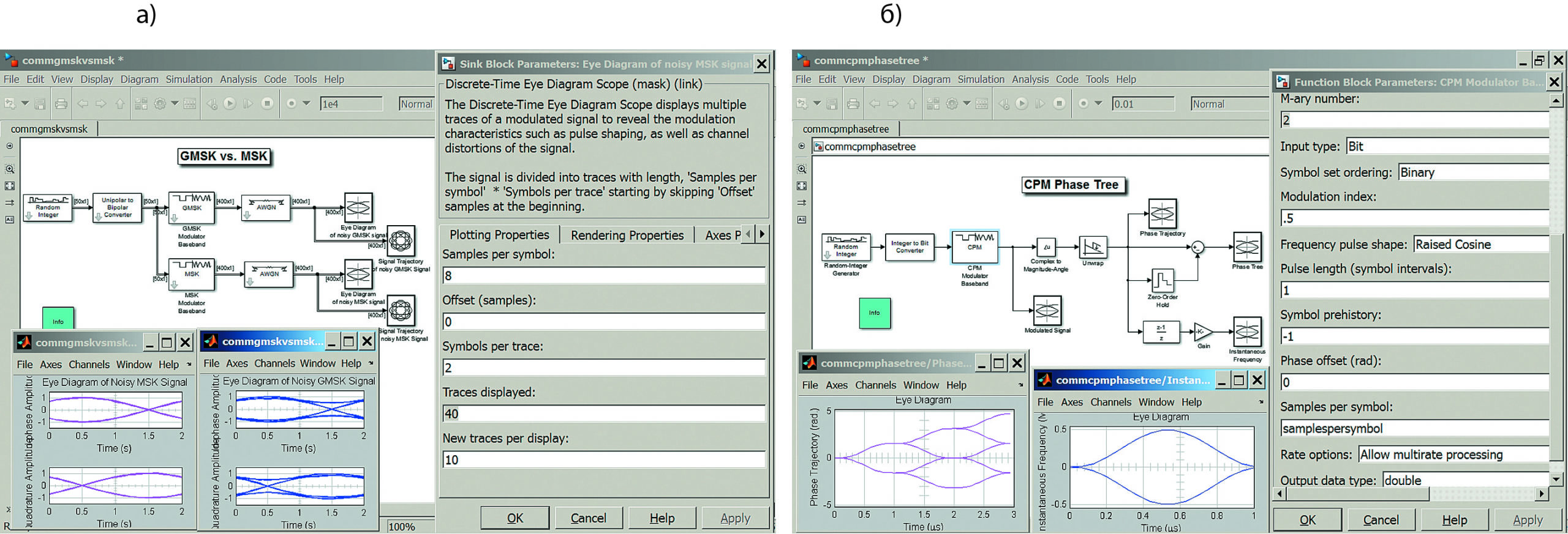
Рис. 10. Диаграмма Simulink:
а) модели с «глазковыми» диаграммами;
б) модели построения фазового дерева
Еще один пример создания «глазковых» диаграмм приведен на рис. 10б. Одна из «глазковых» диаграмм строит фазовое дерево. Такие диаграммы обычно применяются для представления многокомпонентных сигналов.
Реализация манипуляции с минимальным фазовым сдвигом с применением аппарата операций с плавающей точкой показана на рис. 11. Эти операции выполняются на аппаратном уровне, что позволяет уменьшить время моделирования.

Рис. 11. Диаграмма со спектром сигнала и сложными звездными диаграммами
Моделирование узлов коммутационных систем
Пакет расширения Communications System Toolbox позволяет моделировать различные узлы коммуникационных систем. На рис. 12 показана диаграмма модели цифрового синтезатора частоты. Его частота определяется высокостабильной частотой обычного кварцевого опорного генератора, умноженной на M и деленной на частоту делителя частоты N. Используется система фазовой автоподстройки управляемого напряжением генератора. Результат преобразуется в симметричные прямоугольные импульсы — меандр (он изображен слева под диаграммой модели).

Рис. 12. Диаграмма модели цифрового синтезатора частоты
В подобных синтезаторах частоты, часто реализованных в виде специальных интегральных микросхем, особое значение имеет время выхода на установившийся режим работы при включении схемы и переключении ее частоты (осциллограмма справа под диаграммой модели). Это время может быть малым, что обеспечивает решение с применением таких синтезаторов в широком круге практических задач.
В современных системах связи часто используются адаптивные эквалайзеры (рис. 13). Эквалайзер обычно корректирует характеристики коммутационных систем, обеспечивая минимум ошибок и повышенную надежность работы систем.

Рис. 13. Диаграмма модели адаптивного эквалайзера LMS, RLS и CMA
Сейчас мы не будем вникать в особенности работы эквалайзера. Графическая иллюстрация работы адаптивного эквалайзера представлена на рис. 14. Хорошо видна сложность работы этого устройства и обилие представляющих ее графиков различного типа. Их анализ, безусловно, полезен тем, кто исследует и разрабатывает подобные устройства.

Рис. 14. Графическая иллюстрация работы эквалайзера, представленного на рис. 13
Применение адаптивного эквалайзера в линии связи показано на рис. 15. Алгоритм работы эквалайзера реализован функцией MATLAB. В справке по пакету описано несколько вариантов построения и применения эквалайзеров.

Рис. 15. Адаптивный эквалайзер в линии связи
Моделирование проводной коммуникационной системы ADSL
Максимальная скорость модемов в начале внедрения Интернета составляла 56–64 кбит/c и была ограничена обычным способом передачи сигналов по телефонным линиям. Со временем оказалось, что эта скорость может быть повышена на 2–3 порядка при использовании волнового принципа передачи сигналов высокочастотной области спектра, передаваемых по обычным телефонным линиям. Так появились проводные системы широкополосной связи ISDN, а позже ADSL (рис. 17) [6]. Такие системы используют многотоновые сигналы и принцип частотного разделения данных при их передаче и приеме.

Рис. 16. 256 канальный дискретный многотоновый сигнал в ADSL
На рис. 16 показан спектр сигнала в ADSL-линии. Диаграмма модели многотонового модулятора приведена на рис. 17. Система сохраняет в низкочастотной области все возможности обычной телефонной связи и добавляет множество новых возможностей, например распараллеливание телефонной связи, службу контроля номеров вызывающего абонента и др. Правда, в данной модели эти возможности не моделируются.

Рис. 17. Диаграмма модели многотонового модулятора системы ADSL
Моделирование процессов в коммуникационных устройствах
В коммуникационных системах происходят сложные процессы во всех областях определения сигналов — энергетической (амплитудной), временной, частотной, фазовой и логической (цифровой). Сложность этих процессов нередко вынуждает разработчиков коммутационных систем исследовать их по частям и моделировать даже отдельные процессы. Система MATLAB с пакетом расширения Communications System Toolbox приспособлена для этого.
На рис. 18 показано моделирование фазового шума в 256‑канальной системе связи с квадратурной амплитудной модуляцией. Хорошо видно, что шум значительно увеличивает число битовых ошибок и искажает звездную диаграмму. При этом звездочки превращаются в черточки.

Рис. 18. Эффекты фазового шума при 256 QAM
Диаграмма моделирования системы синхронизации представлена на рис. 19. Не вдаваясь в тонкости работы системы синхронизации, отметим лишь резкое нарастание ошибок в начале процесса, когда синхронизация еще не установилась. Пожалуй, самое ценное при таком моделировании — исследование переходных процессов в ходе синхронизации и оценка характера и времени переходных процессов при синхронизации.

Рис. 19. Диаграмма моделирования синхронизации
С помощью особых методов кодирования и ввода избыточных кодов можно создавать системы с защитой от ошибок. Пример моделирования одной из таких систем приведен на рис. 20.

Рис. 20. Организация защищенных коммуникаций
Иногда полезно моделирование коммуникационных систем на физическом уровне. Несколько таких примеров дано в справке по описываемому пакету. На рис. 21 показан один из них.

Рис. 21. Анализ WDCMA на уровне физического слоя
Результаты моделирования на этом уровне часто отличаются обилием различных графиков и осциллограмм (рис. 22). Это является признаком сложности процессов, происходящих в коммуникационных системах.

Рис. 22. Графическая иллюстрация процессов на уровне физического слоя
Канальная интерференция существенно влияет на качество передачи информации в системах связи. На рис. 23 показано это обстоятельство на примере интерференции в каналах.

Рис. 23. Канальная интерференция
В телеграфии и радиотелеграфии особое значение имеет передача по линиям связи символьных сигналов. На рис. 24 показана диаграмма модели передачи символа Гарднера, именуемого «собачкой» и применяемого в написании адресов электронной почты. Здесь используется M‑PSK-модулятор и PSK-демодулятор.

Рис. 24. Диаграмма модели передачи символа Гарднера
Моделирование полных коммуникационных систем
Важное место занимает моделирование полных коммуникационных систем, имеющих передатчик, каналы связи и приемник. На рис. 28 показана диаграмма модели такой системы ADSL, основанной на асимметричном частотном методе полос передачи и приема сигналов данных по обычному телефонному кабелю. Этот вид связи применяется до сих пор (в том числе для предоставления услуг Интернета на умеренных скоростях в полосе частот от 0 до 4 кГц) [7].
На рис. 25 приведена диаграмма модели 256‑канальной коммуникационной системы ADSL. Представлены блоки передатчика (Transmitter) и приемника (Receiver) этой системы из блоков, входящих в состав пакета Communications System Toolbox: это позволяет резко упростить моделирование подобных систем.

Рис. 25. Диаграмма модели 256 канальной коммуникационной системы ADSL
Еще одна диаграмма полной модели коммуникационной системы с квадратурно-позиционной модуляцией QPSK показана на рис. 26. Приведены также результаты работы этой системы, представленные многочисленными диаграммами и осциллограммами, полученными от виртуальных приборов.

Рис. 26. Диаграмма модели коммуникационной системы QPSK
Моделирование беспроводных систем коммуникаций Bluetooth
Наличие большого числа различных блоков, порою решающих сложные функциональные задачи, позволяет осуществить макромоделирование и моделирование современных беспроводных систем коммуникаций, например, таких как Bluetooth и Wi-Fi [6]. Эти системы работают на СВЧ и благодаря широкому распространению реализованы в виде твердотельных интегральных микросхем. Они функционируют на небольших расстояниях (десятки-сотни метров), и на их работу существенное влияние оказывают стены и расположение комнат в зданиях, различные препятствия на пути распространения радиоволн и прочие факторы.
На рис. 27 показана диаграмма беспроводной системы связи Bluetooth со скачкообразным изменением частоты (Frequency Hopping). Скорость изменения частоты достигает 1600 скачков в секунду, а скорость передачи данных — до 1 Мбит. Передача данных идет в частотном диапазоне 2,4 ГГц на малые расстояния (десятки метров). Системы Bluetooth широко применяются для связи между компьютерами, сотовыми телефонами и другими офисными, промышленными и медицинскими аппаратами. Обратите внимание на отсутствие ошибок при большом объеме передаваемой информации.

Рис. 27. Диаграмма модели беспроводной Bluetooth коммуникационной системы
Система беспроводной связи Bluetooth неплохо справляется с передачей звуковой информации и изображений, например с одного мобильного устройства на другое. Пример такой передачи показан на рис. 28.

Рис. 28. Диаграмма модели голосовой Bluetooth-связи
Моделирование систем связи стандарта Wi-Fi
Еще более широкими возможностями обладают беспроводные сети класса Wi-Fi. Пакет Communications System Toolbox имеет достаточный набор блоков, чтобы моделировать современные сети Wi-Fi, например стандартов IEEE 812.11. На рис. 29 показана диаграмма модели линии связи IEEE 812.11a (WLAN) на уровне физического слоя. Модель поддерживает скорости передачи данных в 6, 9, 12, 18, 24, 36, 48 и 54 Мбит/c.

Рис. 29. Диаграмма модели линии связи IEEE 812.11a
Графическая иллюстрация работы системы IEEE 812.11a представлена на рис. 30 и отличается разнообразием диаграмм и спектров. Они, разумеется, полезны специалистам по разработке и эксплуатации таких систем.

Рис. 30. Графическая иллюстрация работы IEEE 812.11a
Моделирование систем связи стандарта WiMAX
Стандарт IEEE 802.16, названный WiMAX (Worldwide Interoperability for Microwave Access — «международное взаимодействие для микроволнового доступа»), был разработан для организации единых беспроводных сетей в городском масштабе — WMAN (Wireless Metropolitan Area Network) [6]. Группа стандартов WiMAX позволяет осуществлять беспроводную связь на расстоянии до 50 км, то есть даже вне зоны прямой видимости. Система используется во всем мире с пользовательской скоростью передачи данных до 75 Мбит/c. Диаграмма модели IEEE 802.16 2004 представлена на рис. 31.

Рис. 31. Диаграмма модели IEEE 802.16 2004
На рис. 32 показана диаграмма WiMAX с блоком кодирования, улучшающим показатели системы. В России WiMAX находится в начале своего развития.

Рис. 32. Диаграмма модели IEEE 802.16 2004 с блоком кодирования
Моделирование системы спутниковой связи
Спутниковые системы связи также можно моделировать в пакете расширения Communications System Toolbox. Примером может служить диаграмма модели такой системы, показанная на рис. 33. Она использует вид манипуляции 16‑QAM (16‑позиционная система квадратурной амплитудной манипуляции).

Рис. 33. Диаграмма модели спутниковой системы связи
Единые средства анализа и визуализации коммуникационных систем
Представленные выше средства анализа и визуализации коммуникационных систем, применяемые в матричной системе MATLAB, в настоящее время внедряются в новейшие измерительные приборы — цифровые осциллографы (в том числе многодоменные), измерительные генераторы, анализаторы спектра, цепей и сигналов [7]. Это создает единую основу для исследования, проектирования и моделирования современных коммуникационных устройств и систем. MATLAB является идеальной системой для освоения этих средств инженерно-техническими и научными работниками и студентами технических вузов соответствующего профиля.
На рис. 34, к примеру, представлен экран анализатора спектра реального времени корпорации Tektronix серии 6100 с графическими диаграммами и спектром. Они подобны приведенным выше и созданным в системе MATLAB+Simulink 8.0 с пакетом расширения Communications System Toolbox. Но стоимость анализатора спектра на порядок выше стоимости системы MATLAB+Simulink с полным набором пакетов расширения. Поэтому ее применение для проектирования и изучения коммуникационных систем представляется вполне оправданным экономически, актуальным и своевременным, хотя конечным этапом разработки всегда является реальное «железо».

Рис. 34. Реальные графические диаграммы на экране современного анализатора спектра поразительно схожи с диаграммами пакета расширения Communications System Toolbox системы MATLAB+Simulink 8.0 (R2012b)
Заключение
Пакет расширения Communications System Toolbox содержит многочисленные средства (в том числе Simulink-блоки) разнообразных компонентов и систем связи и коммуникаций, работающих по созданным в последние годы стандартам, в частности, ADSL, Bluetooth, Wi-Fi, WiMAX, спутниковой связи и др. Все они превратились в массовые изделия, применяемые во всем мире и реализованные на вполне доступных интегральных микросхемах. Таким образом, MATLAB+Simulink 8.0 (R2012b) стала одной из первых перспективных систем для проектирования и моделирования современных линий связи и коммуникационных систем. Возможности по моделированию генераторов, модуляторов, демодуляторов и т. д., а также по представлению и индикации сигналов позволяют выполнять в этой системе широкий спектр работ.
Литература
- mathworks.com
- Дьяконов В. П. MATLAB R2006/2007/2008 + Simulink 5/6/7. Основы применения. М.: СОЛОН-Пресс, 2008.
- Дьяконов В. П. MATLAB. Полный самоучитель. М.: ДМК-Пресс, 2012.
- Дьяконов В. П. MATLAB и Simulink для радиоинженеров. М.: ДМК-Пресс, 2011.
- Дьяконов В. П. MATLAB 2011b в обработке сигналов и моделировании электронных устройств // Компоненты и технологии. 2012. № 2.
- Дьяконов В. П., Образцов А. А., Смердов В. Ю. Электронные средства связи. М.: СОЛОН-Пресс, 2005.
- Афонский А. А., Дьяконов В. П. Электронные измерения в нанотехнологиях и в микроэлектронике. М.: ДМК-Пресс, 2011.