This topic describes how to compute error statistics for various communications
systems.
Computation of Theoretical Error Statistics
The biterr function, discussed in the
Compute SERs and BERs Using Simulated Data section, can help you gather empirical error
statistics, but validating your results by comparing them to the theoretical error
statistics is good practice. For certain types of communications systems,
closed-form expressions exist for the computation of the bit error rate (BER) or an
approximate bound on the BER. The functions listed in this table compute the
closed-form expressions for the BER or a bound on it for the specified types of
communications systems.
| Type of Communications System | Function |
|---|---|
| Uncoded AWGN channel | berawgn
|
| Uncoded Rayleigh and Rician fading channel | berfading
|
| Coded AWGN channel | bercoding |
| Uncoded AWGN channel with imperfect synchronization | bersync
|
The analytical expressions used in these functions are discussed in
Analytical Expressions Used in BER Analysis. The reference pages of these functions also list
references to one or more books containing the closed-form expressions implemented
by the function.
Theoretical Performance Results
-
Plot Theoretical Error Rates
-
Compare Theoretical and Empirical Error Rates
Plot Theoretical Error Rates
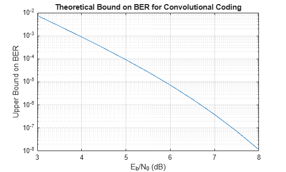
This example uses the bercoding function to compute upper bounds on BERs for convolutional coding with a soft-decision decoder.
coderate = 1/4; % Code rate
Create a structure, dspec, with information about the distance spectrum. Define the energy per bit to noise power spectral density ratio (Eb/N0) sweep range and generate the theoretical bound results.
dspec.dfree = 10; % Minimum free distance of code
dspec.weight = [1 0 4 0 12 0 32 0 80 0 192 0 448 0 1024 ...
    0 2304 0 5120 0]; % Distance spectrum of code
EbNo = 3:0.5:8;
berbound = bercoding(EbNo,'conv','soft',coderate,dspec);
Plot the theoretical bound results.
semilogy(EbNo,berbound)
xlabel('E_b/N_0 (dB)');
ylabel('Upper Bound on BER');
title('Theoretical Bound on BER for Convolutional Coding');
grid on;
Compare Theoretical and Empirical Error Rates
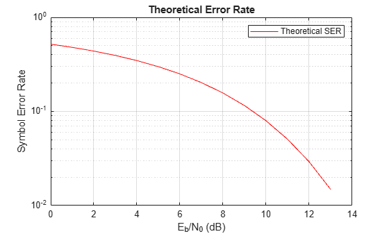
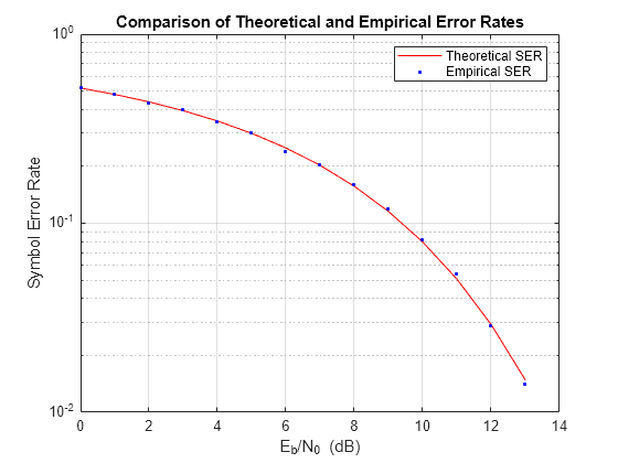
Using the berawgn function, compute the theoretical symbol error rates (SERs) for pulse amplitude modulation (PAM) over a range of Eb/N0 values. Simulate 8 PAM with an AWGN channel, and compute the empirical SERs. Compare the theoretical and then empirical SERs by plotting them on the same set of axes.
Compute and plot the theoretical SER using berawgn.
rng('default') % Set random number seed for repeatability
M = 8;
EbNo = 0:13;
[ber,ser] = berawgn(EbNo,'pam',M);

semilogy(EbNo,ser,'r');
legend('Theoretical SER');
title('Theoretical Error Rate');
xlabel('E_b/N_0 (dB)');
ylabel('Symbol Error Rate');
grid on;
Compute the empirical SER by simulating an 8 PAM communications system link. Define simulation parameters and preallocate variables needed for the results. As described in [1], because N0=2×(NVariance)2, add 3 dB to the Eb/N0 value when converting Eb/N0 values to SNR values.
n = 10000; % Number of symbols to process
k = log2(M); % Number of bits per symbol
snr = EbNo+3+10*log10(k); % In dB
ynoisy = zeros(n,length(snr));
z = zeros(n,length(snr));
errVec = zeros(3,length(EbNo));
Create an error rate calculator System object™ to compare decoded symbols to the original transmitted symbols.
errcalc = comm.ErrorRate;
Generate a random data message and apply PAM. Normalize the channel to the signal power. Loop the simulation to generate error rates over the range of SNR values.
x = randi([0 M-1],n,1); % Create message signal
y = pammod(x,M); % Modulate
signalpower = (real(y)'*real(y))/length(real(y));

for jj = 1:length(snr)
    reset(errcalc)
    ynoisy(:,jj) = awgn(real(y),snr(jj),'measured'); % Add AWGN
    z(:,jj) = pamdemod(complex(ynoisy(:,jj)),M); % Demodulate
    errVec(:,jj) = errcalc(x,z(:,jj)); % Compute SER from simulation
end
Compare the theoretical and empirical results.
hold on;
semilogy(EbNo,errVec(1,:),'b.');
legend('Theoretical SER','Empirical SER');
title('Comparison of Theoretical and Empirical Error Rates');
hold off;
Performance Results via Simulation
-
Section Overview
-
Compute SERs and BERs Using Simulated Data
Section Overview
This section describes how to compare the data messages that enter and leave
a communications system simulation and how to compute error statistics using the
Monte Carlo technique. Simulations can measure system performance by using the
data messages before transmission and after reception to compute the BER or SER
for a communications system. To explore physical layer components used to model
and simulate communications systems, see PHY Components.
Curve fitting can be useful when you have a small or imperfect data set but
want to plot a smooth curve for presentation purposes. To explore the use of
curve fitting when computing performance results via simulation, see the Curve Fitting for Error Rate Plots section.
Compute SERs and BERs Using Simulated Data
The example shows how to compute SERs and BERs using the biterr and symerr functions, respectively. The symerr function compares two sets of data and computes the number of symbol errors and the SER. The biterr function compares two sets of data and computes the number of bit errors and the BER. An error is a discrepancy between corresponding points in the two sets of data.
The two sets of data typically represent messages entering a transmitter and recovered messages leaving a receiver. You can also compare data entering and leaving other parts of your communications system (for example, data entering an encoder and data leaving a decoder).
If your communications system uses several bits to represent one symbol, counting symbol errors is different from counting bit errors. In either the symbol- or bit-counting case, the error rate is the number of errors divided by the total number of transmitted symbols or bits, respectively.
Typically, simulating enough data to produce at least 100 errors provides accurate error rate results. If the error rate is very small (for example, 10-6 or less), using the semianalytic technique might compute the result more quickly than using a simulation-only approach. For more information, see the Performance Results via Semianalytic Technique section.
Compute Error Rates
Use the symerr function to compute the SERs for a noisy linear block code. Apply no digital modulation, so that each symbol contains a single bit. When each symbol is a single bit, the symbol errors and bit errors are the same.
After artificially adding noise to the encoded message, compare the resulting noisy code to the original code. Then, decode and compare the decoded message to the original message.
m = 3; % Set parameters for Hamming code
n = 2^m-1;
k = n-m;
msg = randi([0 1],k*200,1); % Specify 200 messages of k bits each
code = encode(msg,n,k,'hamming');
codenoisy = bsc(code,0.95); % Add noise
newmsg = decode(codenoisy,n,k,'hamming'); % Decode and correct errors
Compute the SERs.
[~,noisyVec] = symerr(code,codenoisy);
[~,decodedVec] = symerr(msg,newmsg);
The error rate decreases after decoding because the Hamming decoder correct errors based on the error-correcting capability of the decoder configuration. Because random number generators produce the message and noise is added, results vary from run to run. Display the SERs.
disp(['SER in the received code: ',num2str(noisyVec(1))])
SER in the received code: 0.94571
disp(['SER after decoding: ',num2str(decodedVec(1))])
SER after decoding: 0.9675
Comparing SER and BER
These commands show the difference between symbol errors and bit errors in various situations.
Create two three-element decimal vectors and show the binary representation. The vector a contains three 2-bit symbols, and the vector b contains three 3-bit symbols.
bpi = 3; % Bits per integer
a = [1 2 3];
b = [1 4 4];
int2bit(a,bpi)
ans = 3×3

     0     0     0
     0     1     1
     1     0     1
ans = 3×3

     0     1     1
     0     0     0
     1     0     0
Compare the binary values of the two vectors and compute the number of errors and the error rate by using the biterr and symerr functions.
format rat % Display fractions instead of decimals
[snum,srate] = symerr(a,b)
snum is 2 because the second and third entries have bit differences. srate is 2/3 because the total number of symbols is 3.
[bnum,brate] = biterr(a,b)
bnum is 5 because the second entries differ in two bits, and the third entries differ in three bits. brate is 5/9 because the total number of bits is 9. By definition, the total number of bits is the number of entries in a for symbol error computations or b for bit error computations times the maximum number of bits among all entries of a and b, respectively.
Performance Results via Semianalytic Technique
The technique described in the Performance Results via Simulation
section can work for a large variety of communications systems but can be
prohibitively time-consuming for small error rates (for example,
10-6 or less). The semianalytic technique is an
alternative way to compute error rates. The semianalytic technique can produce
results faster than a nonanalytic method that uses simulated data.
For more information on implementing the semianalytic technique using a
combination of simulation and analysis to determine the error rate of a
communications system, see the semianalytic function.
Error Rate Plots
-
Section Overview
-
Creation of Error Rate Plots Using
semilogy
Function -
Curve Fitting for Error Rate Plots
-
Use Curve Fitting on Error Rate Plot
Section Overview
Error rate plots can be useful when examining the performance of a
communications system and are often included in publications. This section
discusses and demonstrates tools you can use to create error rate plots, modify
them to suit your needs, and perform curve fitting on the error rate data and
the plots.
Creation of Error Rate Plots Using semilogy Function
In many error rate plots, the horizontal axis indicates
Eb/N0
values in dB, and the vertical axis indicates the error rate using a logarithmic
(base 10) scale. For examples that create such a plot using the semilogy function, see Compare Theoretical and Empirical Error Rates and Plot Theoretical Error Rates.
Curve Fitting for Error Rate Plots
Curve fitting can be useful when you have a small or imperfect data set but
want to plot a smooth curve for presentation purposes. The berfit function includes
curve-fitting capabilities that help your analysis when the empirical data
describes error rates at different
Eb/N0
values. This function enables you to:
-
Customize various relevant aspects of the curve-fitting process, such
as a list of selections for the type of closed-form function used to
generate the fit. -
Plot empirical data along with a curve that
berfitfits to the
data. -
Interpolate points on the fitted curve between
Eb/N0
values in your empirical data set to smooth the plot. -
Collect relevant information about the fit, such as the numerical
values of points along the fitted curve and the coefficients of the fit
expression.
Note
The berfit function is
intended for curve fitting or interpolation, not extrapolation.
Extrapolating BER data beyond an order of magnitude below the smallest
empirical BER value is inherently unreliable.
Use Curve Fitting on Error Rate Plot
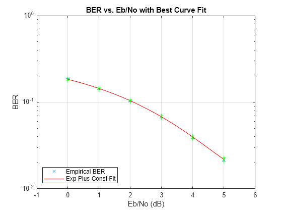
This example simulates a simple differential binary phase shift keying (DBPSK) communications system and plots error rate data for a series of Eb/N0 values. It uses the berfit and berconfint functions to fit a curve to a set of empirical error rates.
Initialize Simulation Parameters
Specify the input signal message length, modulation order, range of Eb/N0 values to simulate, and the minimum number of errors that must occur before the simulation computes an error rate for a given Eb/N0 value. Preallocate variables for final results and interim results.
Typically, for statistically accurate error rate results, the minimum number of errors must be on the order of 100. This simulation uses a small number of errors to shorten the run time and to illustrate how curve fitting can smooth a set of results.
siglen = 100000; % Number of bits in each trial
M = 2; % DBPSK is binary
EbN0vec = 0:5; % Vector of EbN0 values
minnumerr = 5; % Compute BER after only 5 errors occur
numEbN0 = length(EbN0vec); % Number of EbN0 values

ber = zeros(1,numEbN0); % Final BER values
berVec = zeros(3,numEbN0); % Updated BER values
intv = cell(1,numEbN0); % Cell array of confidence intervals
Create an error rate calculator System object™.
errorCalc = comm.ErrorRate;
Loop the Simulation
Simulate the DBPSK-modulated communications system and compute the BER using a for loop to vary the Eb/N0 value. The inner while loop ensures that a minimum number of bit errors occur for each Eb/N0 value. Error rate statistics are saved for each Eb/N0 value and used later in this example when curve fitting and plotting.
for jj = 1:numEbN0
    EbN0 = EbN0vec(jj);
    snr = EbN0; % For binary modulation SNR = EbN0
    reset(errorCalc)

    while (berVec(2,jj) < minnumerr)
        msg = randi([0,M-1],siglen,1); % Generate message sequence
        txsig = dpskmod(msg,M); % Modulate
        rxsig = awgn(txsig,snr,'measured'); % Add noise
        decodmsg = dpskdemod(rxsig,M); % Demodulate
        berVec(:,jj) = errorCalc(msg,decodmsg); % Calculate BER
    end
Use the berconfint function to compute the error rate at a 98% confidence interval for the Eb/N0 values.
    [ber(jj),intv1] = berconfint(berVec(2,jj),berVec(3,jj),0.98);
    intv{jj} = intv1;
    disp(['EbN0 = ' num2str(EbN0) ' dB, ' num2str(berVec(2,jj)) ...
        ' errors, BER = ' num2str(ber(jj))])
end
EbN0 = 0 dB, 18392 errors, BER = 0.18392
EbN0 = 1 dB, 14307 errors, BER = 0.14307
EbN0 = 2 dB, 10190 errors, BER = 0.1019
EbN0 = 3 dB, 6940 errors, BER = 0.0694
EbN0 = 4 dB, 4151 errors, BER = 0.04151
EbN0 = 5 dB, 2098 errors, BER = 0.02098
Use the berfit function to plot the best fitted curve, interpolating between BER points to get a smooth plot. Add confidence intervals to the plot.
fitEbN0 = EbN0vec(1):0.25:EbN0vec(end); % Interpolation values
berfit(EbN0vec,ber,fitEbN0);
hold on;
for jj=1:numEbN0
    semilogy([EbN0vec(jj) EbN0vec(jj)],intv{jj},'g-+');
end
hold off;
See Also
Apps
- Bit Error Rate Analysis
Functions
berawgn|bercoding|berconfint|berfading|berfit|bersync
Related Topics
- Analyze Performance with Bit Error Rate Analysis App
- Analytical Expressions Used in BER Analysis
From Wikipedia, the free encyclopedia
In digital transmission, the number of bit errors is the number of received bits of a data stream over a communication channel that have been altered due to noise, interference, distortion or bit synchronization errors.
The bit error rate (BER) is the number of bit errors per unit time. The bit error ratio (also BER) is the number of bit errors divided by the total number of transferred bits during a studied time interval. Bit error ratio is a unitless performance measure, often expressed as a percentage.[1]
The bit error probability pe is the expected value of the bit error ratio. The bit error ratio can be considered as an approximate estimate of the bit error probability. This estimate is accurate for a long time interval and a high number of bit errors.
Example[edit]
As an example, assume this transmitted bit sequence:
1 1 0 0 0 1 0 1 1
and the following received bit sequence:
0 1 0 1 0 1 0 0 1,
The number of bit errors (the underlined bits) is, in this case, 3. The BER is 3 incorrect bits divided by 9 transferred bits, resulting in a BER of 0.333 or 33.3%.
Packet error ratio[edit]
The packet error ratio (PER) is the number of incorrectly received data packets divided by the total number of received packets. A packet is declared incorrect if at least one bit is erroneous. The expectation value of the PER is denoted packet error probability pp, which for a data packet length of N bits can be expressed as
 ,
,

assuming that the bit errors are independent of each other. For small bit error probabilities and large data packets, this is approximately

Similar measurements can be carried out for the transmission of frames, blocks, or symbols.
The above expression can be rearranged to express the corresponding BER (pe) as a function of the PER (pp) and the data packet length N in bits:
![{displaystyle p_{e}=1-{sqrt[{N}]{(1-p_{p})}}}](https://wikimedia.org/api/rest_v1/media/math/render/svg/f5d380e45b0451c45265e199221fae5bd5b84bf9)
Factors affecting the BER[edit]
In a communication system, the receiver side BER may be affected by transmission channel noise, interference, distortion, bit synchronization problems, attenuation, wireless multipath fading, etc.
The BER may be improved by choosing a strong signal strength (unless this causes cross-talk and more bit errors), by choosing a slow and robust modulation scheme or line coding scheme, and by applying channel coding schemes such as redundant forward error correction codes.
The transmission BER is the number of detected bits that are incorrect before error correction, divided by the total number of transferred bits (including redundant error codes). The information BER, approximately equal to the decoding error probability, is the number of decoded bits that remain incorrect after the error correction, divided by the total number of decoded bits (the useful information). Normally the transmission BER is larger than the information BER. The information BER is affected by the strength of the forward error correction code.
Analysis of the BER[edit]
The BER may be evaluated using stochastic (Monte Carlo) computer simulations. If a simple transmission channel model and data source model is assumed, the BER may also be calculated analytically. An example of such a data source model is the Bernoulli source.
Examples of simple channel models used in information theory are:
- Binary symmetric channel (used in analysis of decoding error probability in case of non-bursty bit errors on the transmission channel)
- Additive white Gaussian noise (AWGN) channel without fading.
A worst-case scenario is a completely random channel, where noise totally dominates over the useful signal. This results in a transmission BER of 50% (provided that a Bernoulli binary data source and a binary symmetrical channel are assumed, see below).
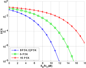
Bit-error rate curves for BPSK, QPSK, 8-PSK and 16-PSK, AWGN channel.

In a noisy channel, the BER is often expressed as a function of the normalized carrier-to-noise ratio measure denoted Eb/N0, (energy per bit to noise power spectral density ratio), or Es/N0 (energy per modulation symbol to noise spectral density).
For example, in the case of QPSK modulation and AWGN channel, the BER as function of the Eb/N0 is given by:
 .[2]
.[2]
People usually plot the BER curves to describe the performance of a digital communication system. In optical communication, BER(dB) vs. Received Power(dBm) is usually used; while in wireless communication, BER(dB) vs. SNR(dB) is used.
Measuring the bit error ratio helps people choose the appropriate forward error correction codes. Since most such codes correct only bit-flips, but not bit-insertions or bit-deletions, the Hamming distance metric is the appropriate way to measure the number of bit errors. Many FEC coders also continuously measure the current BER.
A more general way of measuring the number of bit errors is the Levenshtein distance.
The Levenshtein distance measurement is more appropriate for measuring raw channel performance before frame synchronization, and when using error correction codes designed to correct bit-insertions and bit-deletions, such as Marker Codes and Watermark Codes.[3]
Mathematical draft[edit]
The BER is the likelihood of a bit misinterpretation due to electrical noise  . Considering a bipolar NRZ transmission, we have
 for a «1» and
  for a «0». Each of
  and
and  has a period of
  .
.
Knowing that the noise has a bilateral spectral density  ,
,
is 
and is  .
.
Returning to BER, we have the likelihood of a bit misinterpretation  .
.
 and
and 
where  is the threshold of decision, set to 0 when
  .
.
We can use the average energy of the signal  to find the final expression :

±§
Bit error rate test[edit]
BERT or bit error rate test is a testing method for digital communication circuits that uses predetermined stress patterns consisting of a sequence of logical ones and zeros generated by a test pattern generator.
A BERT typically consists of a test pattern generator and a receiver that can be set to the same pattern. They can be used in pairs, with one at either end of a transmission link, or singularly at one end with a loopback at the remote end. BERTs are typically stand-alone specialised instruments, but can be personal computer–based. In use, the number of errors, if any, are counted and presented as a ratio such as 1 in 1,000,000, or 1 in 1e06.
Common types of BERT stress patterns[edit]
- PRBS (pseudorandom binary sequence) – A pseudorandom binary sequencer of N Bits. These pattern sequences are used to measure jitter and eye mask of TX-Data in electrical and optical data links.
- QRSS (quasi random signal source) – A pseudorandom binary sequencer which generates every combination of a 20-bit word, repeats every 1,048,575 words, and suppresses consecutive zeros to no more than 14. It contains high-density sequences, low-density sequences, and sequences that change from low to high and vice versa. This pattern is also the standard pattern used to measure jitter.
- 3 in 24 – Pattern contains the longest string of consecutive zeros (15) with the lowest ones density (12.5%). This pattern simultaneously stresses minimum ones density and the maximum number of consecutive zeros. The D4 frame format of 3 in 24 may cause a D4 yellow alarm for frame circuits depending on the alignment of one bits to a frame.
- 1:7 – Also referred to as 1 in 8. It has only a single one in an eight-bit repeating sequence. This pattern stresses the minimum ones density of 12.5% and should be used when testing facilities set for B8ZS coding as the 3 in 24 pattern increases to 29.5% when converted to B8ZS.
- Min/max – Pattern rapid sequence changes from low density to high density. Most useful when stressing the repeater’s ALBO feature.
- All ones (or mark) – A pattern composed of ones only. This pattern causes the repeater to consume the maximum amount of power. If DC to the repeater is regulated properly, the repeater will have no trouble transmitting the long ones sequence. This pattern should be used when measuring span power regulation. An unframed all ones pattern is used to indicate an AIS (also known as a blue alarm).
- All zeros – A pattern composed of zeros only. It is effective in finding equipment misoptioned for AMI, such as fiber/radio multiplex low-speed inputs.
- Alternating 0s and 1s — A pattern composed of alternating ones and zeroes.
- 2 in 8 – Pattern contains a maximum of four consecutive zeros. It will not invoke a B8ZS sequence because eight consecutive zeros are required to cause a B8ZS substitution. The pattern is effective in finding equipment misoptioned for B8ZS.
- Bridgetap — Bridge taps within a span can be detected by employing a number of test patterns with a variety of ones and zeros densities. This test generates 21 test patterns and runs for 15 minutes. If a signal error occurs, the span may have one or more bridge taps. This pattern is only effective for T1 spans that transmit the signal raw. Modulation used in HDSL spans negates the bridgetap patterns’ ability to uncover bridge taps.
- Multipat — This test generates five commonly used test patterns to allow DS1 span testing without having to select each test pattern individually. Patterns are: all ones, 1:7, 2 in 8, 3 in 24, and QRSS.
- T1-DALY and 55 OCTET — Each of these patterns contain fifty-five (55), eight bit octets of data in a sequence that changes rapidly between low and high density. These patterns are used primarily to stress the ALBO and equalizer circuitry but they will also stress timing recovery. 55 OCTET has fifteen (15) consecutive zeroes and can only be used unframed without violating one’s density requirements. For framed signals, the T1-DALY pattern should be used. Both patterns will force a B8ZS code in circuits optioned for B8ZS.
Bit error rate tester[edit]
A bit error rate tester (BERT), also known as a «bit error ratio tester»[4] or bit error rate test solution (BERTs) is electronic test equipment used to test the quality of signal transmission of single components or complete systems.
The main building blocks of a BERT are:
- Pattern generator, which transmits a defined test pattern to the DUT or test system
- Error detector connected to the DUT or test system, to count the errors generated by the DUT or test system
- Clock signal generator to synchronize the pattern generator and the error detector
- Digital communication analyser is optional to display the transmitted or received signal
- Electrical-optical converter and optical-electrical converter for testing optical communication signals
See also[edit]
- Burst error
- Error correction code
- Errored second
- Pseudo bit error ratio
- Viterbi Error Rate
References[edit]
- ^ Jit Lim (14 December 2010). «Is BER the bit error ratio or the bit error rate?». EDN. Retrieved 2015-02-16.
- ^
Digital Communications, John Proakis, Massoud Salehi, McGraw-Hill Education, Nov 6, 2007 - ^
«Keyboards and Covert Channels»
by Gaurav Shah, Andres Molina, and Matt Blaze (2006?) - ^ «Bit Error Rate Testing: BER Test BERT » Electronics Notes». www.electronics-notes.com. Retrieved 2020-04-11.
![]() This article incorporates public domain material from Federal Standard 1037C. General Services Administration. (in support of MIL-STD-188).
This article incorporates public domain material from Federal Standard 1037C. General Services Administration. (in support of MIL-STD-188).
External links[edit]
- QPSK BER for AWGN channel – online experiment
The signal-to-noise ratio (SNR) and the resulting BER for a specific modulation format depend on the demodulation scheme employed. This is so because the noise added to the signal is different for different demodulation schemes. In this tutorial we consider the shot-noise limit and discuss BER for the three demodulation schemes discussed in the demodulation schemes tutorial. In the next tutorial we will focus on a more realistic situation in which system performance is limited by other noise sources introduced by lasers and optical amplifiers employed along the fiber link.
1. Synchronous Heterodyne Receivers
Consider first the case of the binary ASK format. The signal used by the decision circuit is given

with φ = 0. The phase difference φ = φs — φLO generally varies randomly because of phase fluctuations associated with the transmitter laser and the local oscillator. We consider such fluctuations later in the next tutorial but neglect them here as our objective is to discuss the shot-noise limit. The decision signal for the ASK format then becomes

where Ip ≡ 2Rd(PsPLO)1/2 takes values I1 and I0 depending on whether a 1 or 0 bit is being detected. We assume no power is transmitted during the 0 bits and set I0 = 0.
Except for the factor of 1/2 in this equation, the situation is analogous to the case of direct detection discussed in the optical receiver sensitivity tutorial. The factor of 1/2 does not affect the BER since both the signal and the noise are reduced by the same factor, leaving the SNR unchanged. In fact, one can use the same result

where the Q factor can be written as

In relating Q to SNR, we used I0 = 0 and set σ0 ≈ σ1. The latter approximation is justified for coherent receivers whose noise is dominated by shot noise induced by the local-oscillator and remains the same irrespective of the received signal power. As shown in the coherent detection tutorial, the SNR can be related to the number of photons Np received during each 1 bit by the simple relation SNR = 2ηNp, where η is the quantum efficiency of the photodetectors employed.
The use of the two equations above with SNR = 2ηNp provides the following expression for the BER:

One can use the same method to calculate the BER in the case of ASK homodyne receivers. The last BER equation and the Q equation above still remain applicable. However, the SNR is improved by 3 dB in the homodyne case.
The last BER equation can be used to calculate the receiver sensitivity at a specific BER. Similar to the direct-detection case discussed in the optical receiver sensitivity tutorial, we define the receiver sensitivity  as the average received power required for realizing a BER of 10-9 or less. From the two equations above, BER = 10-9 when Q ≈ 6, or when SNR = 144 (21.6 dB). We can use the following equation to relate SNR to

if we note that

simply because signal power is zero during the 0 bits. The result is

In the ASK homodyne case, is smaller by a factor of 2 because of the 3-dB homodyne-detection advantage. As an example, for a 1.55-μm ASK heterodyne receiver with η = 0.8 and Δf = 1 GHz, the receiver sensitivity is about 12 nW and reduces to 6 nW if homodyne detection is used.
The receiver sensitivity is often quoted in terms of the number of photons Np using the BER expression above because such a choice makes it independent of the receiver bandwidth and the operating wavelength. Furthermore, η is also set to 1 so that the sensitivity corresponds to an ideal photodetector. It is easy to verify that for realizing a BER of 10-9, Np should be 72 and 36 in the heterodyne and homodyne cases, respectively. It is important to remember that Np corresponds to the number of photons within a single 1 bit. The average number of photons per bit,  , is reduced by a factor of 2 in the case of binary ASK format.
Consider now the case of the BPSK format. The signal at the decision circuit is given by

The main difference from the ASK case is that Ip is constant, but the phase φ takes values 0 or π depending on whether a 1 or 0 is being transmitted. In both cases, Id is a Gaussian random variable but its average value is either Ip/2 or — Ip/2, depending on the received bit. The situation is analogous to the ASK case with the difference that I0 = — I1 in place of being zero. In fact, we can usefor the BER, but Q is now given by

where I0 = — I1 and σ0 = σ1 was used. By using SNR = 2ηNp, the BER is given by

As before, the SNR is improved by 3 dB, or by a factor of 2, in the case of PSK homodyne detection.
The receiver sensitivity at a BER of 10-9 can be obtained by using Q = 6. For the purpose of comparison, it is useful to express the receiver sensitivity in terms of the number of photons Np. It is easy to verify that Np = 18 and 9 for heterodyne and homodyne BPSK detection, respectively. The average number of photons/bit,  , equals Np for the PSK format because the same power is transmitted during 1 and 0 bits. A PSK homodyne receiver is the most sensitive receiver, requiring only 9 photons/bit.
For completeness, consider the case of binary FSK format for which heterodyne receivers employ a dual-filter scheme, each filter passing only 1 or 0 bits. The scheme is equivalent to two complementary ASK heterodyne receivers operating in parallel. This feature allows us to use
for the FSK as well. However, the SNR is improved by a factor of 2 compared with the ASK case because the same amount of power is received even during 0 bits. By using SNR = 4ηNp, the BER is given by

In terms of the number of photons, the sensitivity is given by

The figure below shows the BER as a function of ηNp for the ASK, PSK, and FSK formats, demodulated by using a synchronous heterodyne receiver.

It is interesting to compare the sensitivity of coherent receivers with that of a direct-detection receiver. The table below shows such a comparison.

As discussed in the optical receiver sensitivity tutorial, an ideal direct-detection receiver requires 10 photons/bit to operate at a BER of ≤ 10-9. This value is considerably superior to that of heterodyne schemes. However, it is never achieved in practice because of thermal noise, dark current, and many other factors, which degrade the sensitivity to the extent that

is usually required. In the case of coherent receivers, below 100 can be realized because shot noise can be made dominant by increasing the local-oscillator power.
2. Asynchronous Heterodyne Receivers
The BER calculation for asynchronous receivers is more complicated because the noise does not remain Gaussian when an envelop detector is used. The reason can be understood from this equation showing the signal processed by the decision circuit.

In the case of an ideal ASK heterodyne receiver, φ can be set to zero so that (subscript d is dropped for simplicity)

Even though both ic and is are Gaussian random variable with zero mean and the same standard deviation σ, where σ is the root mean square (RMS) noise current, the probability density function (PDF) of I is not Gaussian. It can be calculated by using a standard technique and is found to be given by

where I0(x) represents a modified Bessel function of the first kind and I varies in the range 0 to ∞ because the output of an envelop detector can have only positive values. This PDF is known as the Rice distribution. When Ip = 0, the Rice distribution reduces to a Rayleigh distribution, well known in statistical optics.
The BER calculation follows the analysis of the optical receiver sensitivity tutorial with the only difference that the Rice distribution needs to be used in place of the Gaussian distribution. The BER is given by

with

where ID is the decision level and I1 and I0 are values of Ip for 1 and 0 bits. The noise is the same for all bits (σ0 = σ1 = σ) because it is dominated by the local oscillator power. The integrals in the equations can be expressed in terms of Marcum’s Q function, defined as

The result for the BER is

The decision level ID is chosen such that the BER is minimum for given values of I1, I0, and σ. It is difficult to obtain an exact analytic expression of ID. However, under typical operating conditions, I0 ≈ 0, I1/σ ≫ 1, and ID is well approximated by I1/2. The BER then becomes

Using SNR = 2ηNp, we obtain the final result,
A comparison with the following equation,

obtained in the case of synchronous ASK receivers shows that the BER is larger in the asynchronous case for the same value of ηNp. However, the difference is so small that the receiver sensitivity at a BER of 10-9 is degraded by only 0.5 dB. If we assume η = 1,
shows that BER = 10-9 for

while

in the synchronous case.
Consider next the PSK format. As mentioned earlier, asynchronous demodulation cannot be used for it. However, DBPSK signals can be demodulated by implementing the delay-demodulation scheme in the microwave regime. The filtered current in this following equation:

is divided into two parts, and one part is delayed by exactly one symbol period Ts. The product of two currents depends on the phase difference between any two neighboring bits and is used by the decision current to determine the bit pattern.
To find the PDF of the decision variable, we write this equation in the form

where

Here, n = ic + iis is a complex Gaussian random process. The current used by the decision circuit can now be written as

If ωIFTs is chosen to be a multiple of 2π and we can approximate ψ with φ, then Id = ±r(t)r(t — Ts) as the phase difference takes its two values of 0 and π. The BER is thus determined by the PDF of the random variable r(t)r(t — Ts).
It is helpful to write this product in the form

where

Consider the error probability when φ = 0 for which Id > 0 in the absence of noise. An error will occur if r+ < r— because of noise. Thus, the conditional probability is given by

This probability can be calculated because the PDFs of r±2 can be obtained by noting that n(t) and n(t — Ts) are uncorrelated Gaussian random variables. The other conditional probability, P(0|π), can be found in the same manner. The final result is quite simple and is given by

A BER of 10-9 is obtained for ηNp = 20. As a reminder, the quantity ηNp is just the SNR per bit in the shot noise limit.
3. Receivers with Delay Demodulation
In the delay-demodulation scheme shown in the demodulation schemes tutorial, one or more MZ interferometers with one-symbol delay are used at the receiver end. In the DBPSK case, a single MZ interferometer is employed. The outputs of the two detectors in this case have average currents given by

The decision variable is formed by subtracting the two currents such that

The average currents for 0 and 1 bits are RdP0 and — RdP0 for Δφ = 0 and π, respectively.
To see how the noise affects the two currents, note that from this equation

that Id can be written in the form

where

is the optical field entering the receiver. Here, n(t) represent the noise induced by vacuum fluctuations that lead to the shot noise at the receiver. A comparison of this equation with
obtained in the case of heterodyne detector with delay implemented in the microwave domain, shows the similarity between the two cases. Following the discussion presented here, one can conclude that the BER in the DBPSK case is again given by
As before, the SNR per bit, ηNp, sets the BER, and a BER of 10-9 is obtained for ηNp = 20.
The analysis is much more involved in the case of the DQPSK format. Proakis has developed a systematic approach for calculating error probabilities for a variety of modulation formats that includes the DQPSK format. Although his analysis is for a heterodyne receiver with delay implemented in the microwave domain, the results apply as well to the case of optical delay demodulation. In particular, when the DQPSK format is implemented with the Gray coding, the BER is given by

where I0 is the modified Bessel function of order zero and Q1(a, b) is Marcum’s Q function introduced earlier.
The following figure shows the BER curves for the DBPSK and DQPSK formats and compares them with the BER curve obtained in the case in which a heterodyne receiver is employed to detect the BPSK or the QPSK format (without differential encoding).

When DBPSK is used in place of BPSK, the receiver sensitivity at a BER of 10-9 changes from 18 to 20 photons/bit, indicating a power penalty of less than 0.5 dB. In view of a such a small penalty, DBPSK is often used in place of BPSK because its use avoids the need of a local oscillator and simplifies the receiver design considerably. However, a penalty of close to 2.4 dB occurs in the case of DQPSK format for which receiver sensitivity changes from 18 to 31 photons/bit.
Because of the complexity of the BER expression above, it is useful to find its approximate analytic form. Using the upper and lower bounds on Marcum’s Q function, this BER expression can be written in the following simple form

This expression is accurate to within 1% for BER values below 3 x 10⁻². If we now employ asymptotic expansions

valid for large values of x, and use a and b from

we obtain

This expression is accurate to within a few percent for values of ηNp > 3.
Having built a simple digital communication system, it is necessary to know how to measure its performance. As the names say, Symbol Error Rate (SER) and Bit Error Rate (BER) are the probabilities of receiving a symbol and bit in error, respectively. SER and BER can be approximated through simulating a complete digital communication system involving a large number of bits and comparing the ratio of symbols or bits received in error to the total number of bits. Hence,
begin{equation}label{eqCommSystemSER}
text{SER} = frac{text{No. of symbols in error}}{text{Total no. of transmitted symbols}}
end{equation}
and
begin{equation}label{eqCommSystemBER}
text{BER} = frac{text{No. of bits in error}}{text{Total no. of transmitted bits}}
end{equation}
Till now, the only imperfection between Tx and Rx entities we have covered is AWGN. It then makes sense that more distortions should corrupt the signal further and result in more errors. Hence, SER or BER plotted against some measure of signal-to-noise ratio (SNR) is the benchmark against which the performance of a system can be measured. Another useful parameter that combines the effects of all impairments into a single value is Error Vector Magnitude (EVM).
Next, we discuss how we choose a specific measure of SNR against which SER and BER should be plotted.
Figure of Merit: $E_b/N_0$
The SNR in a digital communication system is defined as a ratio of signal power in a symbol $P_M$ to noise power $P_w$ as
begin{equation}label{eqCommSystemSNR}
SNR = frac{P_M}{P_w}
end{equation}
where the signal power $P_M$l is modulation average symbol energy per unit symbol time
begin{equation}label{eqCommSystemPowerEnergy}
P_M = frac{E_M}{T_M}
end{equation}
For PAM and QAM modulation schemes, average $E_M$ was defined in their respective articles, see Pulse Amplitude Modulation (PAM) and Quadrature Amplitude Modulation (QAM). Moreover, how to determine the noise power $P_w$ was detailed in the article on AWGN.
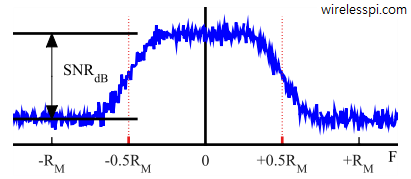
When specified in dB units and using a factor of 10 for power conversions, it is
begin{align}
SNR_{text{dB}} &= P_{M,text{dB}} – P_{w,text{dB}} nonumber \
&= 10 log_{10} P_M – 10log_{10} P_w label{eqCommSystemSNRdB}
end{align}
A visual measure of finding $mathrm{SNR_{dB}}$ is shown in Figure below.
Using Eq eqref{eqCommSystemPowerEnergy} and Eq eqref{eqCommSystemNoisePower1}, notice that the SNR can also be written as
begin{align*}
P_M cdot frac{1}{P_w} &= frac{E_M}{T_M} cdot frac{1}{N_0 B} \
&= E_M R_M cdot frac{1}{N_0B}
end{align*}
The above equation can be rearranged as
begin{equation*}
frac{E_M}{N_0} = frac{P_M}{P_w} cdot frac{B}{R_M}
end{equation*}
Recall that there are $log_2 M$ bits in one symbol,
begin{equation}label{eqCommSystemEMEb}
E_b = frac{1}{log_2M} cdot E_M
end{equation}
where $E_b$ is energy per bit. Similarly, the bit rate is
begin{equation}label{eqCommSystemRMRb}
R_b = log_2 M cdot R_M
end{equation}
Plugging the values for $E_b$ and $R_b$,
begin{equation}label{eqCommSystemEbNo}
frac{E_b}{N_0} = frac{P_M}{P_w} cdot frac{B}{R_b} = text{SNR} cdot frac{B}{R_b}
end{equation}
So we can say that $E_b/N_0$ is equal to SNR scaled by ratio of bandwidth to bit rate.
Now the question is: why is $E_b/N_0$ a natural figure of merit in digital communication systems instead of SNR.
- Intuitively, the ratio of signal power $P_M$ to noise power $P_w$ in the system (i.e., SNR) should be a good criterion for measuring performance of different communication systems. And indeed it is true for analog communication systems where the signal continuity transcends the need to partition the signal into some units of time. On the other hand, a symbol is the basic building block of a digital communication system and signal energy within each symbol turns out to be a more useful parameter.
- As we saw in the article on packing more bits in one symbol, many bits ($log_2M$ to be precise) can be packed into every symbol for an $M$-symbol modulation. Consequently, within every $T_M$ seconds, either 1 bit is travelling through the air (BPSK), or 2 bits (QPSK, 4-PAM), or 4 bits (16-QAM, 16-PSK), and so on. As shown in Eq eqref{eqCommSystemEbNo}, using $E_b/N_0$ instead of SNR automatically incorporates this bits per symbol factor through $R_b$.
- Again from Eq eqref{eqCommSystemEbNo}, bandwidth is also taken into account. A system using less bandwidth than the other will have this factor reflected in its $E_b/N_0$ values.
In summary, $E_b/N_0$ is a normalized SNR measure, which proves really useful when comparing the SER/BER performance of digital modulation schemes with different bits per symbol and bandwidths.
The ratio $E_b/N_0$ is dimensionless as
begin{equation*}
frac{E_b}{N_0} = frac{text{Joules}}{text{Watts/Hz}} = frac{text{Watts} cdot text{seconds}}{text{Watts} cdot text{seconds}}
end{equation*}
It is frequently expressed in decibels as $10log_{10} E_b/N_0$.
Scaling Factors
In most of the figures in this text, you would have noticed a very clear labeling on the x-axis. On the y-axis though, the emphasis has been on the shape rather than the exact values. Now when the SER/BER measurements are to be taken, scaling factors on y-axis become equally important.
Constellation
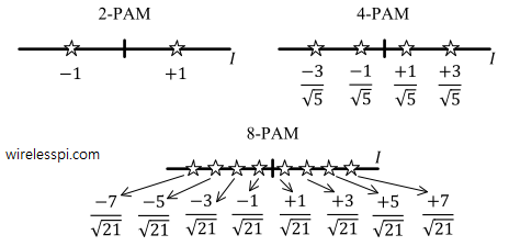
Starting with the symbol constellations, we scale the values such that the average energy per symbol is 1. This can be achieved by dividing the constellation values by the square root of average symbol energy (sum of squares of the constellation points). For example, for a PAM modulation with $A=1$, $E_M$ was shown to be equal to
begin{equation*}
E_{M-text{PAM}} = frac{M^2-1}{3}
end{equation*}
which yields
begin{align*}
E_{2-text{PAM}} &= 1 \
E_{4-text{PAM}} &= 5 \
E_{8-text{PAM}} &= 21 \
vdots
end{align*}
When the constellation points $pm 1$, $pm 3$, $pm 5$, $cdots$, are divided by respective $sqrt{E_M}$, various $M$-PAM constellations become normalized to have average symbol energy equal to $1$, as illustrated in Figure below.
As a verification, consider from Figure above,
begin{align*}
E_{2-text{PAM,norm}} &= frac{1}{2}left(1^2 + 1^2right) = 1 \
E_{4-text{PAM,norm}} &= frac{1}{4}cdot frac{1}{5}left(-3^2 + -1^2 + 1^2 + 3^2 right) = frac{1}{20}cdot 20 = 1 \
E_{8-text{PAM,norm}} &= 1
end{align*}
where the subscript `norm’ stands for normalized.
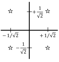
On a similar note, the scaling factor for QAM with $A=1$ was shown as
begin{equation*}
E_{M-text{QAM}} = frac{2}{3} left(M-1right)
end{equation*}
which yields
begin{align*}
E_{4-text{QAM}} &= 2 \
E_{16-text{QAM}} &= 10 \
E_{64-text{QAM}} &= 42 \
vdots
end{align*}
For example, when scaled with square-root of this normalization factor, a normalized $4$-QAM constellation is shown in Figure below. Here, using Pythagoras theorem and realizing that all $4$ symbols have equal energies,
begin{equation*}
E_{4-text{QAM,norm}} = frac{1}{4}cdot 4cdot left(frac{1}{2} + frac{1}{2} right) = 1
end{equation*}
System Design Tradeoffs
Observe that the constellation points come closer to each other for higher-order modulation and normalized average symbol energy. This emphasizes the fact that higher bit rate $R_b$, or more bits per symbol, does not come for free. The tradeoffs involved are
- Power needs to be increased for a fixed bandwidth, because more energy within the same symbol time is needed for maintaining a similar distance between constellation points, or
- Bandwidth needs to be expanded to accommodate a higher symbol rate for fixed power, because same energy then becomes available to spend during a shorter amount of time, or
- An increased error rate needs to accepted for fixed power and bandwidth.
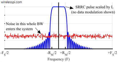
Tx Pulse
To understand the scaling factor for Tx pulse shape, also known as Tx filter, consider the block diagram of a PAM modulator or a QAM modulator. The next step after converting bits to symbols is upsampling the symbol train before it is filtered by a square-root Nyquist filter. This square-root Nyquist filter performs two operations:
- It lowpass filters the spectral replicas arising as a result of increasing the sample rate, see the post on sample rate conversion for details.
- It shapes the symbol sequence so that it is bandlimited in the frequency domain according to given specifications.
We also discussed in sample rate conversion that to maintain the same peak time domain amplitude in the upsampled signal as before, the filter should be designed with a gain equal to the upsampling factor, $L$ in this case. The three available choices, time domain amplitudes and energies were presented there. When we choose this option, the symbol energy gets scaled by $L$ as well as derived in that post. Therefore, denoting energy/symbol in the upsampled and filtered case with $E’_M$,
begin{equation}label{eqCommSystemScalingEnergy}
E_M’ = L cdot E_{Mtext{,norm}} = L
end{equation}
Remember from the post on pulse shaping filter that the peak value in a Square-Root Raised Cosine filter is $1 – alpha + 4alpha/pi$. In an actual implementation of the system, the pulse coefficients should be scaled by this value as well so that the peak value becomes unity and the precision with which the coefficients are represented in a fixed-point arithmetic processor can be maintained. However, here the purpose is only to simulate the BER due to which we ignore this factor.
Noise Power
In the article on AWGN, the noise power $P_w$ within a bandwidth $B$ was derived as
begin{equation}label{eqCommSystemNoisePower1}
P_w = N_0B
end{equation}
For a discrete signal with sampling rate $F_S$, it is understood that the bandwidth has already been constrained by an analog filter within the range $pm 0.5F_S$ to avoid aliasing. Plugging $B=0.5F_S$ in the above equation, the noise power in a sampled bandlimited system is given as
begin{equation*}
P_w = N_0cdot frac{F_S}{2}
end{equation*}
A digital modulation signal is sampled at rate $F_S = L cdot R_M$ where $L$ is samples/symbol. Bit rate $R_b$ can change with different modulation schemes and sample rate $F_S$ can be increased or decreased during the processing chain. On the other hand, the symbol rate $R_M$ is a standard parameter which is directly proportional to the signal bandwidth as shown in the modulation bandwidths, and hence it remains constant throughout the system implementation. For this reason, $R_M$ in most simulation systems is chosen to be equal to $1$ and the other parameters can be scaled accordingly. Then,
begin{equation}
P_w = N_0cdot frac{L}{2} label{eqCommSystemNoisePower2}
end{equation}
Finally, the relationship between noise power $P_w$ and $E_b/N_0$ can be written as
begin{equation*}
P_w = frac{E_b}{E_b/N_0} cdot frac{L}{2}
end{equation*}
which can be modified using $log_2 M$ bits per symbol,
begin{equation}label{eqCommSystemNoisePower3}
P_w = frac{E_M}{log_2 M cdot E_b/N_0} cdot frac{L}{2}
end{equation}
where $E_M$ is the symbol energy. In case normalized energy is used for symbol constellations, it can be replaced with $1$.
Notice that noise power increases by a factor of $L$ due to oversampling the signal. On the other hand, the signal energy increases by a factor of $L$ due to scaling shown in Eq eqref{eqCommSystemScalingEnergy}. The overall result is that both factors cancel out in the numerator and denominator of SNR expression in Eq eqref{eqCommSystemSNR}. This is illustrated in Figure below.
Rx Pulse
Both the signal and noise enter the system before filtered by the Rx pulse. Therefore, any scaling has no effect on the SNR and it only changes the time domain amplitudes. Since the Raised Cosine pulse is a convolution of Tx and Rx Square-Root Raised Cosine pulses defined above, it has a peak amplitude of $1$ and hence maps the symbols exactly on the constellation.
Finally, remember that the group delay defined in pulse shaping filter is now given by the contribution from both Tx and Rx square-root Nyquist filters. For that reason, we remove $LG/2+LG/2=LG$ samples at the start and $LG$ samples at the end of the received sequence.
BER Plots
Now we are at a stage where we can plot the symbol and bit error rates of all three modulation schemes discussed above, namely PAM, QAM and PSK. To avoid any confusion, we leave SER plots and just concentrate on BER plots. SER plots are an obvious byproduct of the simulation setup discussed above.
The BER plots for 2, 4 and 8-PAM modulation are shown in Figure below.

Note that for a fixed $E_b/N_0$, the BER increases with $M$ because the same symbol energy has to be divided among $log_2M$ bits. Similarly, for a fixed BER, more energy is required as $M$ increases to maintain similar distances among constellation points. As an example, for a target BER of $10^{-4}$,
- $E_b/N_0$ needed by $2$-PAM is $8.4$ dB,
- $E_b/N_0$ needed by $4$-PAM is $12.2$ dB,
- $E_b/N_0$ needed by $8$-PAM is $16.5$ dB,
A gray code is a method of assigning bits to symbols in a manner that adjacent symbols differ in only one bit. For example, symbols in a $4$-PAM constellation can be assigned bits 00, 01, 11 and 10 (as opposed to 00,01,10 and 11) such that all symbols have neighbours with only one bit difference. Since Gaussian noise has a higher probability around the mean value, the most likely symbol errors end up in adjacent symbols. As a result, these most likely symbol errors produce one erroneous bit and remaining $M-1$ correct bits. Hence, the relation between BER and SER can be defined as
begin{equation*}
text{BER} = frac {1}{log_2 M} text{SER}
end{equation*}
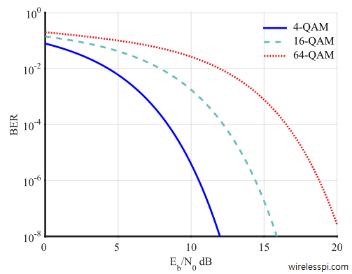
Moving on to QAM, the BER plots for $4$, $16$ and $64$-QAM modulation are shown in Figure beow. Similar conclusions hold for BER vs $E_b/N_0$ as in the case of PAM.
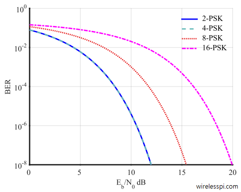
Finally, the BER plots for 2, 4 ,8 and 16-PSK modulation are shown in Figure below. Notice that the plots for BPSK and QPSK overlap with each other because QPSK can be regarded as a pair of orthogonal BPSK systems. We will have more to say about this point in the next section.
Spectral Efficiency
In BER vs $E_b/N_0$ plots above, we noticed that for a target BER of $10^{-4}$, $E_b/N_0$ required by $2$-PAM, $4$-PAM and $8$-PAM are $8.4$ dB, $12.2$ dB and $16.5$ dB, respectively. Does this mean that $8$-PAM is $8$ dB worse than $2$-PAM modulation scheme? The answer is no, because the bandwidth has not been taken into consideration in this comparison. For the same symbol rate (which means same bandwidth), $8$-PAM transmits $3$ bits of information as compared to just $1$ bit of information by $2$-PAM.
For that reason, bandwidth must also be considered to get a complete picture of how different modulations compare to one another. Thus, spectral efficiency is defined as the ratio of bit rate to the bandwidth and its units are bits/s/Hz.
begin{equation}label{eqCommSystemSpectralEfficiency}
text{SE} = frac{R_b}{B} quad text{bits/s/Hz}
end{equation}
In essence, spectral efficiency is a way to figure out how fast the system is per unit of bandwidth. For QAM and PSK constellations with a square-root Nyquist filter of excess bandwidth $alpha$, we saw in the post on modulation bandwidths that the required bandwidth is $(1+alpha)R_M$. In terms of bit rate,
begin{equation*}
B_{text{QAM}} = left(1+alpharight) frac{R_b}{log_2 M}
end{equation*}
from which spectral efficiency can be determined as
begin{equation}label{eqCommSystemSEQAM}
SE_{text{QAM}} = frac{log_2 M}{1+alpha} quad text{bits/s/Hz}
end{equation}
BER for BPSK and QPSK
Going back to our discussion on similar BER for BPSK and QPSK, note that the BPSK system conveys one bit per symbol interval $T_M$, whereas the QPSK system conveys two bits per symbol interval. For a given symbol rate $R_M$ (and hence the same bandwidth) and a given signal power, QPSK has to divide the energy into two bits resulting in smaller $E_b/N_0$ ratio and higher BER. However, its bit rate $R_b$ is twice as compared to BPSK.
On the other hand, for a given bit rate $R_b$ and a given signal power, QPSK symbol interval $T_M$ is twice as long as that of the BPSK, similar energy is available per unit time and hence both BPSK and QPSK have the same BER. However, its symbol rate $R_M$ is half and so it uses half the bandwidth as compared to BPSK.
Turning towards PAM, although the bandwidth required is half as compared to QAM, it transmits half the number of bits as well due to using $I$ channel only. Therefore, its spectral efficiency is similar to QAM.
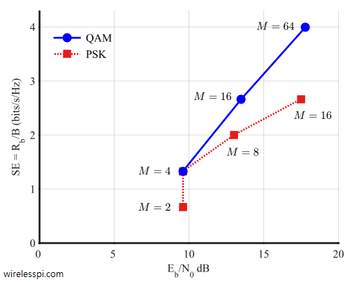
Different constellations with different number of points can be compared by taking all the parameters into account, namely bits/symbol, bandwidth and SNR performance. This can be achieved by plotting the spectral efficiency against the value of $E_b/N_0$ required to obtain a specific target BER. Figure below shows spectral efficiency versus $E_b/N_0$ for QAM and PSK constellations for BER = $10^{-5}$ and excess bandwidth $alpha = 0.5$, where $E_b/N_0$ values can be taken from the x-axis of BER curves in the previous section. Note that QAM provides better spectral efficiency than PSK because it packs the constellation points in a more efficient manner. This is why it is the modulation of choice in most of the high-speed wireless networks today.
In general, better modulations operate at high spectral efficiency and low $E_b/N_0$, i.e., to the top left of this curve.
On a final note, we rewrite Eq eqref{eqCommSystemEbNo} here.
begin{equation*}
frac{E_b}{N_0} = frac{P_M}{P_w} cdot frac{B}{R_b} = text{SNR} cdot frac{B}{R_b}
end{equation*}
The above equation can be written as
begin{equation*}
text{SE} = frac{R_b}{B} = frac{text{SNR}}{E_b/N_0}
end{equation*}
As a result, SE can also be seen as the ratio of SNR to $E_b/N_0$. Thus, the lesser $E_b/N_0$ a modulation scheme requires for a given error rate, the more spectrally efficient it is.