From Wikipedia, the free encyclopedia
In statistics, the mean squared error (MSE)[1] or mean squared deviation (MSD) of an estimator (of a procedure for estimating an unobserved quantity) measures the average of the squares of the errors—that is, the average squared difference between the estimated values and the actual value. MSE is a risk function, corresponding to the expected value of the squared error loss.[2] The fact that MSE is almost always strictly positive (and not zero) is because of randomness or because the estimator does not account for information that could produce a more accurate estimate.[3] In machine learning, specifically empirical risk minimization, MSE may refer to the empirical risk (the average loss on an observed data set), as an estimate of the true MSE (the true risk: the average loss on the actual population distribution).
The MSE is a measure of the quality of an estimator. As it is derived from the square of Euclidean distance, it is always a positive value that decreases as the error approaches zero.
The MSE is the second moment (about the origin) of the error, and thus incorporates both the variance of the estimator (how widely spread the estimates are from one data sample to another) and its bias (how far off the average estimated value is from the true value).[citation needed] For an unbiased estimator, the MSE is the variance of the estimator. Like the variance, MSE has the same units of measurement as the square of the quantity being estimated. In an analogy to standard deviation, taking the square root of MSE yields the root-mean-square error or root-mean-square deviation (RMSE or RMSD), which has the same units as the quantity being estimated; for an unbiased estimator, the RMSE is the square root of the variance, known as the standard error.
Definition and basic properties[edit]
The MSE either assesses the quality of a predictor (i.e., a function mapping arbitrary inputs to a sample of values of some random variable), or of an estimator (i.e., a mathematical function mapping a sample of data to an estimate of a parameter of the population from which the data is sampled). The definition of an MSE differs according to whether one is describing a predictor or an estimator.
Predictor[edit]
If a vector of  predictions is generated from a sample of data points on all variables, and
  is the vector of observed values of the variable being predicted, with
  being the predicted values (e.g. as from a least-squares fit), then the within-sample MSE of the predictor is computed as

In other words, the MSE is the mean  of the squares of the errors
  . This is an easily computable quantity for a particular sample (and hence is sample-dependent).
In matrix notation,

where  is
is  and
and  is the
  column vector.
The MSE can also be computed on q data points that were not used in estimating the model, either because they were held back for this purpose, or because these data have been newly obtained. Within this process, known as statistical learning, the MSE is often called the test MSE,[4] and is computed as

Estimator[edit]
The MSE of an estimator  with respect to an unknown parameter
  is defined as[1]
![{displaystyle operatorname {MSE} ({hat {theta }})=operatorname {E} _{theta }left[({hat {theta }}-theta )^{2}right].}](https://wikimedia.org/api/rest_v1/media/math/render/svg/9a0e1b3bac58f9ba2d2f4ff8b85b2e35a8f4bf78)
This definition depends on the unknown parameter, but the MSE is a priori a property of an estimator. The MSE could be a function of unknown parameters, in which case any estimator of the MSE based on estimates of these parameters would be a function of the data (and thus a random variable). If the estimator is derived as a sample statistic and is used to estimate some population parameter, then the expectation is with respect to the sampling distribution of the sample statistic.
The MSE can be written as the sum of the variance of the estimator and the squared bias of the estimator, providing a useful way to calculate the MSE and implying that in the case of unbiased estimators, the MSE and variance are equivalent.[5]

Proof of variance and bias relationship[edit]
![{displaystyle {begin{aligned}operatorname {MSE} ({hat {theta }})&=operatorname {E} _{theta }left[({hat {theta }}-theta )^{2}right]\&=operatorname {E} _{theta }left[left({hat {theta }}-operatorname {E} _{theta }[{hat {theta }}]+operatorname {E} _{theta }[{hat {theta }}]-theta right)^{2}right]\&=operatorname {E} _{theta }left[left({hat {theta }}-operatorname {E} _{theta }[{hat {theta }}]right)^{2}+2left({hat {theta }}-operatorname {E} _{theta }[{hat {theta }}]right)left(operatorname {E} _{theta }[{hat {theta }}]-theta right)+left(operatorname {E} _{theta }[{hat {theta }}]-theta right)^{2}right]\&=operatorname {E} _{theta }left[left({hat {theta }}-operatorname {E} _{theta }[{hat {theta }}]right)^{2}right]+operatorname {E} _{theta }left[2left({hat {theta }}-operatorname {E} _{theta }[{hat {theta }}]right)left(operatorname {E} _{theta }[{hat {theta }}]-theta right)right]+operatorname {E} _{theta }left[left(operatorname {E} _{theta }[{hat {theta }}]-theta right)^{2}right]\&=operatorname {E} _{theta }left[left({hat {theta }}-operatorname {E} _{theta }[{hat {theta }}]right)^{2}right]+2left(operatorname {E} _{theta }[{hat {theta }}]-theta right)operatorname {E} _{theta }left[{hat {theta }}-operatorname {E} _{theta }[{hat {theta }}]right]+left(operatorname {E} _{theta }[{hat {theta }}]-theta right)^{2}&&operatorname {E} _{theta }[{hat {theta }}]-theta ={text{const.}}\&=operatorname {E} _{theta }left[left({hat {theta }}-operatorname {E} _{theta }[{hat {theta }}]right)^{2}right]+2left(operatorname {E} _{theta }[{hat {theta }}]-theta right)left(operatorname {E} _{theta }[{hat {theta }}]-operatorname {E} _{theta }[{hat {theta }}]right)+left(operatorname {E} _{theta }[{hat {theta }}]-theta right)^{2}&&operatorname {E} _{theta }[{hat {theta }}]={text{const.}}\&=operatorname {E} _{theta }left[left({hat {theta }}-operatorname {E} _{theta }[{hat {theta }}]right)^{2}right]+left(operatorname {E} _{theta }[{hat {theta }}]-theta right)^{2}\&=operatorname {Var} _{theta }({hat {theta }})+operatorname {Bias} _{theta }({hat {theta }},theta )^{2}end{aligned}}}](https://wikimedia.org/api/rest_v1/media/math/render/svg/2ac524a751828f971013e1297a33ca1cc4c38cd6)
An even shorter proof can be achieved using the well-known formula that for a random variable  ,
,  . By substituting with,
  , we have
![{displaystyle {begin{aligned}operatorname {MSE} ({hat {theta }})&=mathbb {E} [({hat {theta }}-theta )^{2}]\&=operatorname {Var} ({hat {theta }}-theta )+(mathbb {E} [{hat {theta }}-theta ])^{2}\&=operatorname {Var} ({hat {theta }})+operatorname {Bias} ^{2}({hat {theta }})end{aligned}}}](https://wikimedia.org/api/rest_v1/media/math/render/svg/864646cf4426e2b62a3caf9460382eec1a77fe4e)
But in real modeling case, MSE could be described as the addition of model variance, model bias, and irreducible uncertainty (see Bias–variance tradeoff). According to the relationship, the MSE of the estimators could be simply used for the efficiency comparison, which includes the information of estimator variance and bias. This is called MSE criterion.
In regression[edit]
In regression analysis, plotting is a more natural way to view the overall trend of the whole data. The mean of the distance from each point to the predicted regression model can be calculated, and shown as the mean squared error. The squaring is critical to reduce the complexity with negative signs. To minimize MSE, the model could be more accurate, which would mean the model is closer to actual data. One example of a linear regression using this method is the least squares method—which evaluates appropriateness of linear regression model to model bivariate dataset,[6] but whose limitation is related to known distribution of the data.
The term mean squared error is sometimes used to refer to the unbiased estimate of error variance: the residual sum of squares divided by the number of degrees of freedom. This definition for a known, computed quantity differs from the above definition for the computed MSE of a predictor, in that a different denominator is used. The denominator is the sample size reduced by the number of model parameters estimated from the same data, (n−p) for p regressors or (n−p−1) if an intercept is used (see errors and residuals in statistics for more details).[7] Although the MSE (as defined in this article) is not an unbiased estimator of the error variance, it is consistent, given the consistency of the predictor.
In regression analysis, «mean squared error», often referred to as mean squared prediction error or «out-of-sample mean squared error», can also refer to the mean value of the squared deviations of the predictions from the true values, over an out-of-sample test space, generated by a model estimated over a particular sample space. This also is a known, computed quantity, and it varies by sample and by out-of-sample test space.
Examples[edit]
Mean[edit]
Suppose we have a random sample of size from a population,  . Suppose the sample units were chosen with replacement. That is, the units are selected one at a time, and previously selected units are still eligible for selection for all draws. The usual estimator for the
  is the sample average

which has an expected value equal to the true mean (so it is unbiased) and a mean squared error of
![{displaystyle operatorname {MSE} left({overline {X}}right)=operatorname {E} left[left({overline {X}}-mu right)^{2}right]=left({frac {sigma }{sqrt {n}}}right)^{2}={frac {sigma ^{2}}{n}}}](https://wikimedia.org/api/rest_v1/media/math/render/svg/b4647a2cc4c8f9a4c90b628faad2dcf80c4aae84)
where  is the population variance.
For a Gaussian distribution, this is the best unbiased estimator (i.e., one with the lowest MSE among all unbiased estimators), but not, say, for a uniform distribution.
Variance[edit]
The usual estimator for the variance is the corrected sample variance:

This is unbiased (its expected value is ), hence also called the unbiased sample variance, and its MSE is[8]

where  is the fourth central moment of the distribution or population, and
  is the excess kurtosis.
However, one can use other estimators for which are proportional to  , and an appropriate choice can always give a lower mean squared error. If we define

then we calculate:
![{displaystyle {begin{aligned}operatorname {MSE} (S_{a}^{2})&=operatorname {E} left[left({frac {n-1}{a}}S_{n-1}^{2}-sigma ^{2}right)^{2}right]\&=operatorname {E} left[{frac {(n-1)^{2}}{a^{2}}}S_{n-1}^{4}-2left({frac {n-1}{a}}S_{n-1}^{2}right)sigma ^{2}+sigma ^{4}right]\&={frac {(n-1)^{2}}{a^{2}}}operatorname {E} left[S_{n-1}^{4}right]-2left({frac {n-1}{a}}right)operatorname {E} left[S_{n-1}^{2}right]sigma ^{2}+sigma ^{4}\&={frac {(n-1)^{2}}{a^{2}}}operatorname {E} left[S_{n-1}^{4}right]-2left({frac {n-1}{a}}right)sigma ^{4}+sigma ^{4}&&operatorname {E} left[S_{n-1}^{2}right]=sigma ^{2}\&={frac {(n-1)^{2}}{a^{2}}}left({frac {gamma _{2}}{n}}+{frac {n+1}{n-1}}right)sigma ^{4}-2left({frac {n-1}{a}}right)sigma ^{4}+sigma ^{4}&&operatorname {E} left[S_{n-1}^{4}right]=operatorname {MSE} (S_{n-1}^{2})+sigma ^{4}\&={frac {n-1}{na^{2}}}left((n-1)gamma _{2}+n^{2}+nright)sigma ^{4}-2left({frac {n-1}{a}}right)sigma ^{4}+sigma ^{4}end{aligned}}}](https://wikimedia.org/api/rest_v1/media/math/render/svg/cf22322412b8454c706d78671e5d94208675a6e0)
This is minimized when

For a Gaussian distribution, where  , this means that the MSE is minimized when dividing the sum by
  . The minimum excess kurtosis is
  ,[a] which is achieved by a Bernoulli distribution with p = 1/2 (a coin flip), and the MSE is minimized for
  Hence regardless of the kurtosis, we get a «better» estimate (in the sense of having a lower MSE) by scaling down the unbiased estimator a little bit; this is a simple example of a shrinkage estimator: one «shrinks» the estimator towards zero (scales down the unbiased estimator).
Further, while the corrected sample variance is the best unbiased estimator (minimum mean squared error among unbiased estimators) of variance for Gaussian distributions, if the distribution is not Gaussian, then even among unbiased estimators, the best unbiased estimator of the variance may not be 
Gaussian distribution[edit]
The following table gives several estimators of the true parameters of the population, μ and σ2, for the Gaussian case.[9]
| True value | Estimator | Mean squared error |
|---|---|---|
 |
= the unbiased estimator of the population mean,  |

|
 |
= the unbiased estimator of the population variance,  |

|
|
= the biased estimator of the population variance,  |

|
|
= the biased estimator of the population variance,  |

|
Interpretation[edit]
An MSE of zero, meaning that the estimator predicts observations of the parameter with perfect accuracy, is ideal (but typically not possible).
Values of MSE may be used for comparative purposes. Two or more statistical models may be compared using their MSEs—as a measure of how well they explain a given set of observations: An unbiased estimator (estimated from a statistical model) with the smallest variance among all unbiased estimators is the best unbiased estimator or MVUE (Minimum-Variance Unbiased Estimator).
Both analysis of variance and linear regression techniques estimate the MSE as part of the analysis and use the estimated MSE to determine the statistical significance of the factors or predictors under study. The goal of experimental design is to construct experiments in such a way that when the observations are analyzed, the MSE is close to zero relative to the magnitude of at least one of the estimated treatment effects.
In one-way analysis of variance, MSE can be calculated by the division of the sum of squared errors and the degree of freedom. Also, the f-value is the ratio of the mean squared treatment and the MSE.
MSE is also used in several stepwise regression techniques as part of the determination as to how many predictors from a candidate set to include in a model for a given set of observations.
Applications[edit]
- Minimizing MSE is a key criterion in selecting estimators: see minimum mean-square error. Among unbiased estimators, minimizing the MSE is equivalent to minimizing the variance, and the estimator that does this is the minimum variance unbiased estimator. However, a biased estimator may have lower MSE; see estimator bias.
- In statistical modelling the MSE can represent the difference between the actual observations and the observation values predicted by the model. In this context, it is used to determine the extent to which the model fits the data as well as whether removing some explanatory variables is possible without significantly harming the model’s predictive ability.
- In forecasting and prediction, the Brier score is a measure of forecast skill based on MSE.
Loss function[edit]
Squared error loss is one of the most widely used loss functions in statistics[citation needed], though its widespread use stems more from mathematical convenience than considerations of actual loss in applications. Carl Friedrich Gauss, who introduced the use of mean squared error, was aware of its arbitrariness and was in agreement with objections to it on these grounds.[3] The mathematical benefits of mean squared error are particularly evident in its use at analyzing the performance of linear regression, as it allows one to partition the variation in a dataset into variation explained by the model and variation explained by randomness.
Criticism[edit]
The use of mean squared error without question has been criticized by the decision theorist James Berger. Mean squared error is the negative of the expected value of one specific utility function, the quadratic utility function, which may not be the appropriate utility function to use under a given set of circumstances. There are, however, some scenarios where mean squared error can serve as a good approximation to a loss function occurring naturally in an application.[10]
Like variance, mean squared error has the disadvantage of heavily weighting outliers.[11] This is a result of the squaring of each term, which effectively weights large errors more heavily than small ones. This property, undesirable in many applications, has led researchers to use alternatives such as the mean absolute error, or those based on the median.
See also[edit]
- Bias–variance tradeoff
- Hodges’ estimator
- James–Stein estimator
- Mean percentage error
- Mean square quantization error
- Mean square weighted deviation
- Mean squared displacement
- Mean squared prediction error
- Minimum mean square error
- Minimum mean squared error estimator
- Overfitting
- Peak signal-to-noise ratio
Notes[edit]
- ^ This can be proved by Jensen’s inequality as follows. The fourth central moment is an upper bound for the square of variance, so that the least value for their ratio is one, therefore, the least value for the excess kurtosis is −2, achieved, for instance, by a Bernoulli with p=1/2.
References[edit]
- ^ a b «Mean Squared Error (MSE)». www.probabilitycourse.com. Retrieved 2020-09-12.
- ^ Bickel, Peter J.; Doksum, Kjell A. (2015). Mathematical Statistics: Basic Ideas and Selected Topics. Vol. I (Second ed.). p. 20.
If we use quadratic loss, our risk function is called the mean squared error (MSE) …
- ^ a b Lehmann, E. L.; Casella, George (1998). Theory of Point Estimation (2nd ed.). New York: Springer. ISBN 978-0-387-98502-2. MR 1639875.
- ^ Gareth, James; Witten, Daniela; Hastie, Trevor; Tibshirani, Rob (2021). An Introduction to Statistical Learning: with Applications in R. Springer. ISBN 978-1071614174.
- ^ Wackerly, Dennis; Mendenhall, William; Scheaffer, Richard L. (2008). Mathematical Statistics with Applications (7 ed.). Belmont, CA, USA: Thomson Higher Education. ISBN 978-0-495-38508-0.
- ^ A modern introduction to probability and statistics : understanding why and how. Dekking, Michel, 1946-. London: Springer. 2005. ISBN 978-1-85233-896-1. OCLC 262680588.
{{cite book}}: CS1 maint: others (link) - ^ Steel, R.G.D, and Torrie, J. H., Principles and Procedures of Statistics with Special Reference to the Biological Sciences., McGraw Hill, 1960, page 288.
- ^ Mood, A.; Graybill, F.; Boes, D. (1974). Introduction to the Theory of Statistics (3rd ed.). McGraw-Hill. p. 229.
- ^ DeGroot, Morris H. (1980). Probability and Statistics (2nd ed.). Addison-Wesley.
- ^ Berger, James O. (1985). «2.4.2 Certain Standard Loss Functions». Statistical Decision Theory and Bayesian Analysis (2nd ed.). New York: Springer-Verlag. p. 60. ISBN 978-0-387-96098-2. MR 0804611.
- ^ Bermejo, Sergio; Cabestany, Joan (2001). «Oriented principal component analysis for large margin classifiers». Neural Networks. 14 (10): 1447–1461. doi:10.1016/S0893-6080(01)00106-X. PMID 11771723.
From Wikipedia, the free encyclopedia
In statistics, the mean squared error (MSE)[1] or mean squared deviation (MSD) of an estimator (of a procedure for estimating an unobserved quantity) measures the average of the squares of the errors—that is, the average squared difference between the estimated values and the actual value. MSE is a risk function, corresponding to the expected value of the squared error loss.[2] The fact that MSE is almost always strictly positive (and not zero) is because of randomness or because the estimator does not account for information that could produce a more accurate estimate.[3] In machine learning, specifically empirical risk minimization, MSE may refer to the empirical risk (the average loss on an observed data set), as an estimate of the true MSE (the true risk: the average loss on the actual population distribution).
The MSE is a measure of the quality of an estimator. As it is derived from the square of Euclidean distance, it is always a positive value that decreases as the error approaches zero.
The MSE is the second moment (about the origin) of the error, and thus incorporates both the variance of the estimator (how widely spread the estimates are from one data sample to another) and its bias (how far off the average estimated value is from the true value).[citation needed] For an unbiased estimator, the MSE is the variance of the estimator. Like the variance, MSE has the same units of measurement as the square of the quantity being estimated. In an analogy to standard deviation, taking the square root of MSE yields the root-mean-square error or root-mean-square deviation (RMSE or RMSD), which has the same units as the quantity being estimated; for an unbiased estimator, the RMSE is the square root of the variance, known as the standard error.
Definition and basic properties[edit]
The MSE either assesses the quality of a predictor (i.e., a function mapping arbitrary inputs to a sample of values of some random variable), or of an estimator (i.e., a mathematical function mapping a sample of data to an estimate of a parameter of the population from which the data is sampled). The definition of an MSE differs according to whether one is describing a predictor or an estimator.
Predictor[edit]
If a vector of predictions is generated from a sample of data points on all variables, and is the vector of observed values of the variable being predicted, with being the predicted values (e.g. as from a least-squares fit), then the within-sample MSE of the predictor is computed as
In other words, the MSE is the mean of the squares of the errors . This is an easily computable quantity for a particular sample (and hence is sample-dependent).
In matrix notation,
where is and is the column vector.
The MSE can also be computed on q data points that were not used in estimating the model, either because they were held back for this purpose, or because these data have been newly obtained. Within this process, known as statistical learning, the MSE is often called the test MSE,[4] and is computed as
Estimator[edit]
The MSE of an estimator with respect to an unknown parameter is defined as[1]
This definition depends on the unknown parameter, but the MSE is a priori a property of an estimator. The MSE could be a function of unknown parameters, in which case any estimator of the MSE based on estimates of these parameters would be a function of the data (and thus a random variable). If the estimator is derived as a sample statistic and is used to estimate some population parameter, then the expectation is with respect to the sampling distribution of the sample statistic.
The MSE can be written as the sum of the variance of the estimator and the squared bias of the estimator, providing a useful way to calculate the MSE and implying that in the case of unbiased estimators, the MSE and variance are equivalent.[5]
Proof of variance and bias relationship[edit]
An even shorter proof can be achieved using the well-known formula that for a random variable , . By substituting with, , we have
But in real modeling case, MSE could be described as the addition of model variance, model bias, and irreducible uncertainty (see Bias–variance tradeoff). According to the relationship, the MSE of the estimators could be simply used for the efficiency comparison, which includes the information of estimator variance and bias. This is called MSE criterion.
In regression[edit]
In regression analysis, plotting is a more natural way to view the overall trend of the whole data. The mean of the distance from each point to the predicted regression model can be calculated, and shown as the mean squared error. The squaring is critical to reduce the complexity with negative signs. To minimize MSE, the model could be more accurate, which would mean the model is closer to actual data. One example of a linear regression using this method is the least squares method—which evaluates appropriateness of linear regression model to model bivariate dataset,[6] but whose limitation is related to known distribution of the data.
The term mean squared error is sometimes used to refer to the unbiased estimate of error variance: the residual sum of squares divided by the number of degrees of freedom. This definition for a known, computed quantity differs from the above definition for the computed MSE of a predictor, in that a different denominator is used. The denominator is the sample size reduced by the number of model parameters estimated from the same data, (n−p) for p regressors or (n−p−1) if an intercept is used (see errors and residuals in statistics for more details).[7] Although the MSE (as defined in this article) is not an unbiased estimator of the error variance, it is consistent, given the consistency of the predictor.
In regression analysis, «mean squared error», often referred to as mean squared prediction error or «out-of-sample mean squared error», can also refer to the mean value of the squared deviations of the predictions from the true values, over an out-of-sample test space, generated by a model estimated over a particular sample space. This also is a known, computed quantity, and it varies by sample and by out-of-sample test space.
Examples[edit]
Mean[edit]
Suppose we have a random sample of size from a population, . Suppose the sample units were chosen with replacement. That is, the units are selected one at a time, and previously selected units are still eligible for selection for all draws. The usual estimator for the is the sample average
which has an expected value equal to the true mean (so it is unbiased) and a mean squared error of
where is the population variance.
For a Gaussian distribution, this is the best unbiased estimator (i.e., one with the lowest MSE among all unbiased estimators), but not, say, for a uniform distribution.
Variance[edit]
The usual estimator for the variance is the corrected sample variance:
This is unbiased (its expected value is ), hence also called the unbiased sample variance, and its MSE is[8]
where is the fourth central moment of the distribution or population, and is the excess kurtosis.
However, one can use other estimators for which are proportional to , and an appropriate choice can always give a lower mean squared error. If we define
then we calculate:
This is minimized when
For a Gaussian distribution, where , this means that the MSE is minimized when dividing the sum by . The minimum excess kurtosis is ,[a] which is achieved by a Bernoulli distribution with p = 1/2 (a coin flip), and the MSE is minimized for Hence regardless of the kurtosis, we get a «better» estimate (in the sense of having a lower MSE) by scaling down the unbiased estimator a little bit; this is a simple example of a shrinkage estimator: one «shrinks» the estimator towards zero (scales down the unbiased estimator).
Further, while the corrected sample variance is the best unbiased estimator (minimum mean squared error among unbiased estimators) of variance for Gaussian distributions, if the distribution is not Gaussian, then even among unbiased estimators, the best unbiased estimator of the variance may not be
Gaussian distribution[edit]
The following table gives several estimators of the true parameters of the population, μ and σ2, for the Gaussian case.[9]
| True value | Estimator | Mean squared error |
|---|---|---|
|
= the unbiased estimator of the population mean, |
|
|
= the unbiased estimator of the population variance, |
|
|
= the biased estimator of the population variance, |
|
|
= the biased estimator of the population variance, |
|
Interpretation[edit]
An MSE of zero, meaning that the estimator predicts observations of the parameter with perfect accuracy, is ideal (but typically not possible).
Values of MSE may be used for comparative purposes. Two or more statistical models may be compared using their MSEs—as a measure of how well they explain a given set of observations: An unbiased estimator (estimated from a statistical model) with the smallest variance among all unbiased estimators is the best unbiased estimator or MVUE (Minimum-Variance Unbiased Estimator).
Both analysis of variance and linear regression techniques estimate the MSE as part of the analysis and use the estimated MSE to determine the statistical significance of the factors or predictors under study. The goal of experimental design is to construct experiments in such a way that when the observations are analyzed, the MSE is close to zero relative to the magnitude of at least one of the estimated treatment effects.
In one-way analysis of variance, MSE can be calculated by the division of the sum of squared errors and the degree of freedom. Also, the f-value is the ratio of the mean squared treatment and the MSE.
MSE is also used in several stepwise regression techniques as part of the determination as to how many predictors from a candidate set to include in a model for a given set of observations.
Applications[edit]
- Minimizing MSE is a key criterion in selecting estimators: see minimum mean-square error. Among unbiased estimators, minimizing the MSE is equivalent to minimizing the variance, and the estimator that does this is the minimum variance unbiased estimator. However, a biased estimator may have lower MSE; see estimator bias.
- In statistical modelling the MSE can represent the difference between the actual observations and the observation values predicted by the model. In this context, it is used to determine the extent to which the model fits the data as well as whether removing some explanatory variables is possible without significantly harming the model’s predictive ability.
- In forecasting and prediction, the Brier score is a measure of forecast skill based on MSE.
Loss function[edit]
Squared error loss is one of the most widely used loss functions in statistics[citation needed], though its widespread use stems more from mathematical convenience than considerations of actual loss in applications. Carl Friedrich Gauss, who introduced the use of mean squared error, was aware of its arbitrariness and was in agreement with objections to it on these grounds.[3] The mathematical benefits of mean squared error are particularly evident in its use at analyzing the performance of linear regression, as it allows one to partition the variation in a dataset into variation explained by the model and variation explained by randomness.
Criticism[edit]
The use of mean squared error without question has been criticized by the decision theorist James Berger. Mean squared error is the negative of the expected value of one specific utility function, the quadratic utility function, which may not be the appropriate utility function to use under a given set of circumstances. There are, however, some scenarios where mean squared error can serve as a good approximation to a loss function occurring naturally in an application.[10]
Like variance, mean squared error has the disadvantage of heavily weighting outliers.[11] This is a result of the squaring of each term, which effectively weights large errors more heavily than small ones. This property, undesirable in many applications, has led researchers to use alternatives such as the mean absolute error, or those based on the median.
See also[edit]
- Bias–variance tradeoff
- Hodges’ estimator
- James–Stein estimator
- Mean percentage error
- Mean square quantization error
- Mean square weighted deviation
- Mean squared displacement
- Mean squared prediction error
- Minimum mean square error
- Minimum mean squared error estimator
- Overfitting
- Peak signal-to-noise ratio
Notes[edit]
- ^ This can be proved by Jensen’s inequality as follows. The fourth central moment is an upper bound for the square of variance, so that the least value for their ratio is one, therefore, the least value for the excess kurtosis is −2, achieved, for instance, by a Bernoulli with p=1/2.
References[edit]
- ^ a b «Mean Squared Error (MSE)». www.probabilitycourse.com. Retrieved 2020-09-12.
- ^ Bickel, Peter J.; Doksum, Kjell A. (2015). Mathematical Statistics: Basic Ideas and Selected Topics. Vol. I (Second ed.). p. 20.
If we use quadratic loss, our risk function is called the mean squared error (MSE) …
- ^ a b Lehmann, E. L.; Casella, George (1998). Theory of Point Estimation (2nd ed.). New York: Springer. ISBN 978-0-387-98502-2. MR 1639875.
- ^ Gareth, James; Witten, Daniela; Hastie, Trevor; Tibshirani, Rob (2021). An Introduction to Statistical Learning: with Applications in R. Springer. ISBN 978-1071614174.
- ^ Wackerly, Dennis; Mendenhall, William; Scheaffer, Richard L. (2008). Mathematical Statistics with Applications (7 ed.). Belmont, CA, USA: Thomson Higher Education. ISBN 978-0-495-38508-0.
- ^ A modern introduction to probability and statistics : understanding why and how. Dekking, Michel, 1946-. London: Springer. 2005. ISBN 978-1-85233-896-1. OCLC 262680588.
{{cite book}}: CS1 maint: others (link) - ^ Steel, R.G.D, and Torrie, J. H., Principles and Procedures of Statistics with Special Reference to the Biological Sciences., McGraw Hill, 1960, page 288.
- ^ Mood, A.; Graybill, F.; Boes, D. (1974). Introduction to the Theory of Statistics (3rd ed.). McGraw-Hill. p. 229.
- ^ DeGroot, Morris H. (1980). Probability and Statistics (2nd ed.). Addison-Wesley.
- ^ Berger, James O. (1985). «2.4.2 Certain Standard Loss Functions». Statistical Decision Theory and Bayesian Analysis (2nd ed.). New York: Springer-Verlag. p. 60. ISBN 978-0-387-96098-2. MR 0804611.
- ^ Bermejo, Sergio; Cabestany, Joan (2001). «Oriented principal component analysis for large margin classifiers». Neural Networks. 14 (10): 1447–1461. doi:10.1016/S0893-6080(01)00106-X. PMID 11771723.
17 авг. 2022 г.
читать 2 мин
Регрессионный анализ — это метод, который мы можем использовать для понимания взаимосвязи между одной или несколькими переменными-предикторами и переменной отклика .
Один из способов оценить, насколько хорошо регрессионная модель соответствует набору данных, — вычислить среднеквадратичную ошибку , которая представляет собой показатель, указывающий нам среднее расстояние между прогнозируемыми значениями из модели и фактическими значениями в наборе данных.
Чем ниже RMSE, тем лучше данная модель может «соответствовать» набору данных.
Формула для нахождения среднеквадратичной ошибки, часто обозначаемая аббревиатурой RMSE , выглядит следующим образом:
СКО = √ Σ(P i – O i ) 2 / n
куда:
- Σ — причудливый символ, означающий «сумма».
- P i — прогнозируемое значение для i -го наблюдения в наборе данных.
- O i — наблюдаемое значение для i -го наблюдения в наборе данных.
- n — размер выборки
В следующем примере показано, как интерпретировать RMSE для данной модели регрессии.
Пример: как интерпретировать RMSE для регрессионной модели
Предположим, мы хотим построить регрессионную модель, которая использует «учебные часы» для прогнозирования «экзаменационного балла» студентов на конкретном вступительном экзамене в колледж.
Мы собираем следующие данные для 15 студентов:
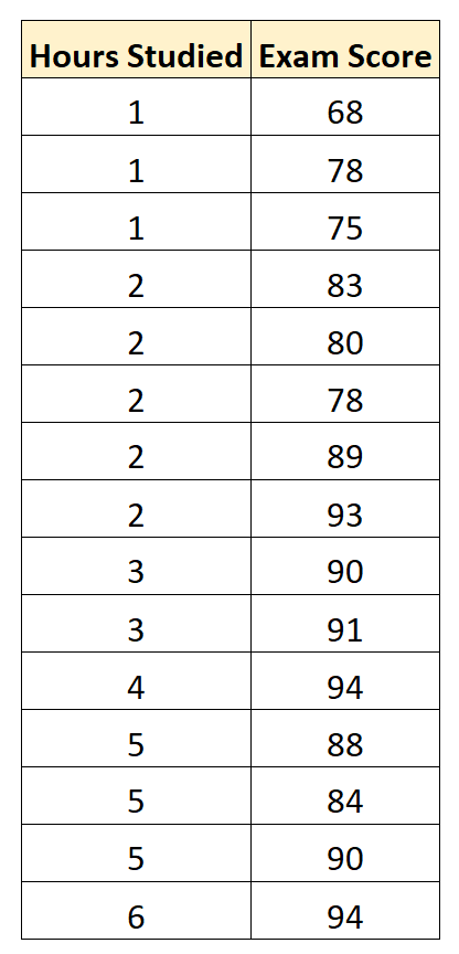
Затем мы используем статистическое программное обеспечение (например, Excel, SPSS, R, Python) и т. д., чтобы найти следующую подогнанную модель регрессии:
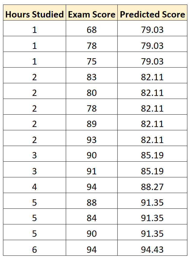
Экзаменационный балл = 75,95 + 3,08 * (часы обучения)
Затем мы можем использовать это уравнение, чтобы предсказать экзаменационную оценку каждого студента, исходя из того, сколько часов они учились:
Затем мы можем вычислить квадрат разницы между каждой прогнозируемой оценкой экзамена и фактической оценкой экзамена. Затем мы можем извлечь квадратный корень из среднего значения этих разностей:
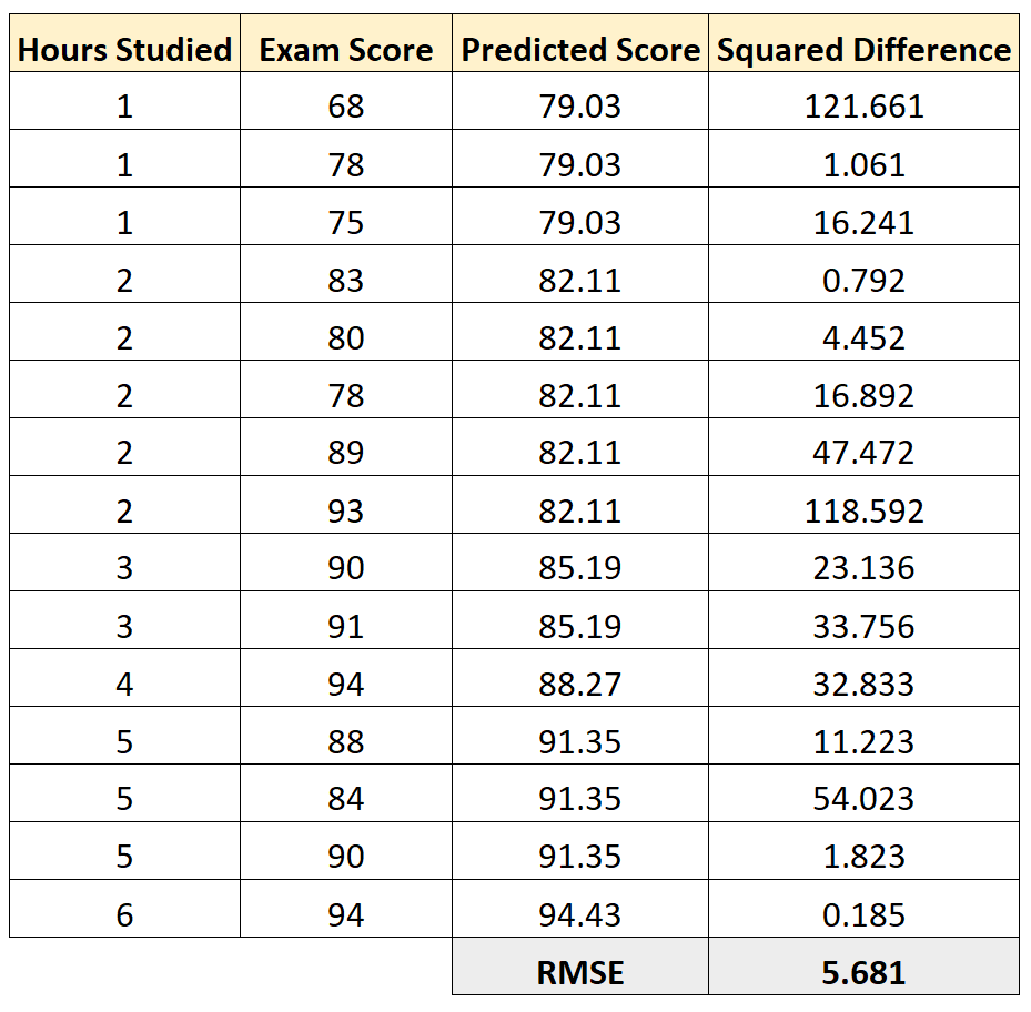
RMSE для этой регрессионной модели оказывается равным 5,681 .
Напомним, что остатки регрессионной модели представляют собой разницу между наблюдаемыми значениями данных и значениями, предсказанными моделью.
Остаток = (P i – O i )
куда
- P i — прогнозируемое значение для i -го наблюдения в наборе данных.
- O i — наблюдаемое значение для i -го наблюдения в наборе данных.
И помните, что RMSE регрессионной модели рассчитывается как:
СКО = √ Σ(P i – O i ) 2 / n
Это означает, что RMSE представляет собой квадратный корень из дисперсии остатков.
Это значение полезно знать, поскольку оно дает нам представление о среднем расстоянии между наблюдаемыми значениями данных и прогнозируемыми значениями данных.
Это отличается от R-квадрата модели, который сообщает нам долю дисперсии переменной отклика, которая может быть объяснена предикторной переменной (переменными) в модели.
Сравнение значений RMSE из разных моделей
RMSE особенно полезен для сравнения соответствия различных моделей регрессии.
Например, предположим, что мы хотим построить регрессионную модель, чтобы предсказать результаты экзаменов студентов, и мы хотим найти наилучшую возможную модель среди нескольких потенциальных моделей.
Предположим, мы подгоняем три разные модели регрессии и находим соответствующие им значения RMSE:
- RMSE модели 1: 14,5
- RMSE модели 2: 16,7
- RMSE модели 3: 9,8
Модель 3 имеет самый низкий RMSE, что говорит нам о том, что она способна лучше всего соответствовать набору данных из трех потенциальных моделей.
Дополнительные ресурсы
Калькулятор среднеквадратичной ошибки
Как рассчитать RMSE в Excel
Как рассчитать RMSE в R
Как рассчитать RMSE в Python
Среднеквадратичная ошибка (Mean Squared Error) – Среднее арифметическое (Mean) квадратов разностей между предсказанными и реальными значениями Модели (Model) Машинного обучения (ML):

Рассчитывается с помощью формулы, которая будет пояснена в примере ниже:
$$MSE = frac{1}{n} × sum_{i=1}^n (y_i — widetilde{y}_i)^2$$
$$MSEspace{}{–}space{Среднеквадратическая}space{ошибка,}$$
$$nspace{}{–}space{количество}space{наблюдений,}$$
$$y_ispace{}{–}space{фактическая}space{координата}space{наблюдения,}$$
$$widetilde{y}_ispace{}{–}space{предсказанная}space{координата}space{наблюдения,}$$
MSE практически никогда не равен нулю, и происходит это из-за элемента случайности в данных или неучитывания Оценочной функцией (Estimator) всех факторов, которые могли бы улучшить предсказательную способность.
Пример. Исследуем линейную регрессию, изображенную на графике выше, и установим величину среднеквадратической Ошибки (Error). Фактические координаты точек-Наблюдений (Observation) выглядят следующим образом:

Мы имеем дело с Линейной регрессией (Linear Regression), потому уравнение, предсказывающее положение записей, можно представить с помощью формулы:
$$y = M * x + b$$
$$yspace{–}space{значение}space{координаты}space{оси}space{y,}$$
$$Mspace{–}space{уклон}space{прямой}$$
$$xspace{–}space{значение}space{координаты}space{оси}space{x,}$$
$$bspace{–}space{смещение}space{прямой}space{относительно}space{начала}space{координат}$$
Параметры M и b уравнения нам, к счастью, известны в данном обучающем примере, и потому уравнение выглядит следующим образом:
$$y = 0,5252 * x + 17,306$$
Зная координаты реальных записей и уравнение линейной регрессии, мы можем восстановить полные координаты предсказанных наблюдений, обозначенных серыми точками на графике выше. Простой подстановкой значения координаты x в уравнение мы рассчитаем значение координаты ỹ:

Рассчитаем квадрат разницы между Y и Ỹ:

Сумма таких квадратов равна 4 445. Осталось только разделить это число на количество наблюдений (9):
$$MSE = frac{1}{9} × 4445 = 493$$
Само по себе число в такой ситуации становится показательным, когда Дата-сайентист (Data Scientist) предпринимает попытки улучшить предсказательную способность модели и сравнивает MSE каждой итерации, выбирая такое уравнение, что сгенерирует наименьшую погрешность в предсказаниях.
MSE и Scikit-learn
Среднеквадратическую ошибку можно вычислить с помощью SkLearn. Для начала импортируем функцию:
import sklearn
from sklearn.metrics import mean_squared_error
Инициализируем крошечные списки, содержащие реальные и предсказанные координаты y:
y_true = [5, 41, 70, 77, 134, 68, 138, 101, 131]
y_pred = [23, 35, 55, 90, 93, 103, 118, 121, 129]
Инициируем функцию mean_squared_error(), которая рассчитает MSE тем же способом, что и формула выше:
mean_squared_error(y_true, y_pred)
Интересно, что конечный результат на 3 отличается от расчетов с помощью Apple Numbers:
496.0Ноутбук, не требующий дополнительной настройки на момент написания статьи, можно скачать здесь.
Автор оригинальной статьи: @mmoshikoo
Фото: @tobyelliott
Для того чтобы модель линейной регрессии можно было применять на практике необходимо сначала оценить её качество. Для этих целей предложен ряд показателей, каждый из которых предназначен для использования в различных ситуациях и имеет свои особенности применения (линейные и нелинейные, устойчивые к аномалиям, абсолютные и относительные, и т.д.). Корректный выбор меры для оценки качества модели является одним из важных факторов успеха в решении задач анализа данных.
- Среднеквадратичная ошибка (Mean Squared Error)
- Корень из среднеквадратичной ошибки (Root Mean Squared Error)
- Среднеквадратичная ошибка в процентах (Mean Squared Percentage Error)
- Cредняя абсолютная ошибка (Mean Absolute Error)
- Средняя абсолютная процентная ошибка (Mean Absolute Percentage Error)
- Cимметричная средняя абсолютная процентная ошибка (Symmetric Mean Absolute Percentage Error)
- Средняя абсолютная масштабированная ошибка (Mean absolute scaled error)
- Средняя относительная ошибка (Mean Relative Error)
- Среднеквадратичная логарифмическая ошибка (Root Mean Squared Logarithmic Error
- R-квадрат
- Скорректированный R-квадрат
- Сравнение метрик
«Хорошая» аналитическая модель должна удовлетворять двум, зачастую противоречивым, требованиям — как можно лучше соответствовать данным и при этом быть удобной для интерпретации пользователем. Действительно, повышение соответствия модели данным как правило связано с её усложнением (в случае регрессии — увеличением числа входных переменных модели). А чем сложнее модель, тем ниже её интерпретируемость.
Поэтому при выборе между простой и сложной моделью последняя должна значимо увеличивать соответствие модели данным чтобы оправдать рост сложности и соответствующее снижение интерпретируемости. Если это условие не выполняется, то следует выбрать более простую модель.
Таким образом, чтобы оценить, насколько повышение сложности модели значимо увеличивает её точность, необходимо использовать аппарат оценки качества регрессионных моделей. Он включает в себя следующие меры:
- Среднеквадратичная ошибка (MSE).
- Корень из среднеквадратичной ошибки (RMSE).
- Среднеквадратичная ошибка в процентах (MSPE).
- Средняя абсолютная ошибка (MAE).
- Средняя абсолютная ошибка в процентах (MAPE).
- Cимметричная средняя абсолютная процентная ошибка (SMAPE).
- Средняя абсолютная масштабированная ошибка (MASE)
- Средняя относительная ошибка (MRE).
- Среднеквадратичная логарифмическая ошибка (RMSLE).
- Коэффициент детерминации R-квадрат.
- Скорректированный коэффициент детеминации.
Прежде чем перейти к изучению метрик качества, введём некоторые базовые понятия, которые нам в этом помогут. Для этого рассмотрим рисунок.
Рисунок 1. Линейная регрессия
Наклонная прямая представляет собой линию регрессии с переменной, на которой расположены точки, соответствующие предсказанным значениям выходной переменной widehat{y} (кружки синего цвета). Оранжевые кружки представляют фактические (наблюдаемые) значения y . Расстояния между ними и линией регрессии — это ошибка предсказания модели y-widehat{y} (невязка, остатки). Именно с её использованием вычисляются все приведённые в статье меры качества.
Горизонтальная линия представляет собой модель простого среднего, где коэффициент при независимой переменной x равен нулю, и остаётся только свободный член b, который становится равным среднему арифметическому фактических значений выходной переменной, т.е. b=overline{y}. Очевидно, что такая модель для любого значения входной переменной будет выдавать одно и то же значение выходной — overline{y}.
В линейной регрессии такая модель рассматривается как «бесполезная», хуже которой работает только «случайный угадыватель». Однако, она используется для оценки, насколько дисперсия фактических значений y относительно линии среднего, больше, чем относительно линии регрессии с переменной, т.е. насколько модель с переменной лучше «бесполезной».
MSE
Среднеквадратичная ошибка (Mean Squared Error) применяется в случаях, когда требуется подчеркнуть большие ошибки и выбрать модель, которая дает меньше именно больших ошибок. Большие значения ошибок становятся заметнее за счет квадратичной зависимости.
Действительно, допустим модель допустила на двух примерах ошибки 5 и 10. В абсолютном выражении они отличаются в два раза, но если их возвести в квадрат, получив 25 и 100 соответственно, то отличие будет уже в четыре раза. Таким образом модель, которая обеспечивает меньшее значение MSE допускает меньше именно больших ошибок.
MSE рассчитывается по формуле:
MSE=frac{1}{n}sumlimits_{i=1}^{n}(y_{i}-widehat{y}_{i})^{2},
где n — количество наблюдений по которым строится модель и количество прогнозов, y_{i} — фактические значение зависимой переменной для i-го наблюдения, widehat{y}_{i} — значение зависимой переменной, предсказанное моделью.
Таким образом, можно сделать вывод, что MSE настроена на отражение влияния именно больших ошибок на качество модели.
Недостатком использования MSE является то, что если на одном или нескольких неудачных примерах, возможно, содержащих аномальные значения будет допущена значительная ошибка, то возведение в квадрат приведёт к ложному выводу, что вся модель работает плохо. С другой стороны, если модель даст небольшие ошибки на большом числе примеров, то может возникнуть обратный эффект — недооценка слабости модели.
RMSE
Корень из среднеквадратичной ошибки (Root Mean Squared Error) вычисляется просто как квадратный корень из MSE:
RMSE=sqrt{frac{1}{n}sumlimits_{i=1}^{n}(y_{i}-widehat{y_{i}})^{2}}
MSE и RMSE могут минимизироваться с помощью одного и того же функционала, поскольку квадратный корень является неубывающей функцией. Например, если у нас есть два набора результатов работы модели, A и B, и MSE для A больше, чем MSE для B, то мы можем быть уверены, что RMSE для A больше RMSE для B. Справедливо и обратное: если MSE(A)<MSE(B), то и RMSE(A)<RMSE(B).
Следовательно, сравнение моделей с помощью RMSE даст такой же результат, что и для MSE. Однако с MSE работать несколько проще, поэтому она более популярна у аналитиков. Кроме этого, имеется небольшая разница между этими двумя ошибками при оптимизации с использованием градиента:
frac{partial RMSE}{partial widehat{y}_{i}}=frac{1}{2sqrt{MSE}}frac{partial MSE}{partial widehat{y}_{i}}
Это означает, что перемещение по градиенту MSE эквивалентно перемещению по градиенту RMSE, но с другой скоростью, и скорость зависит от самой оценки MSE. Таким образом, хотя RMSE и MSE близки с точки зрения оценки моделей, они не являются взаимозаменяемыми при использовании градиента для оптимизации.
Влияние каждой ошибки на RMSE пропорционально величине квадрата ошибки. Поэтому большие ошибки оказывают непропорционально большое влияние на RMSE. Следовательно, RMSE можно считать чувствительной к аномальным значениям.
MSPE
Среднеквадратичная ошибка в процентах (Mean Squared Percentage Error) представляет собой относительную ошибку, где разность между наблюдаемым и фактическим значениями делится на наблюдаемое значение и выражается в процентах:
MSPE=frac{100}{n}sumlimits_{i=1}^{n}left ( frac{y_{i}-widehat{y}_{i}}{y_{i}} right )^{2}
Проблемой при использовании MSPE является то, что, если наблюдаемое значение выходной переменной равно 0, значение ошибки становится неопределённым.
MSPE можно рассматривать как взвешенную версию MSE, где вес обратно пропорционален квадрату наблюдаемого значения. Таким образом, при возрастании наблюдаемых значений ошибка имеет тенденцию уменьшаться.
MAE
Cредняя абсолютная ошибка (Mean Absolute Error) вычисляется следующим образом:
MAE=frac{1}{n}sumlimits_{i=1}^{n}left | y_{i}-widehat{y}_{i} right |
Т.е. MAE рассчитывается как среднее абсолютных разностей между наблюдаемым и предсказанным значениями. В отличие от MSE и RMSE она является линейной оценкой, а это значит, что все ошибки в среднем взвешены одинаково. Например, разница между 0 и 10 будет вдвое больше разницы между 0 и 5. Для MSE и RMSE, как отмечено выше, это не так.
Поэтому MAE широко используется, например, в финансовой сфере, где ошибка в 10 долларов должна интерпретироваться как в два раза худшая, чем ошибка в 5 долларов.
MAPE
Средняя абсолютная процентная ошибка (Mean Absolute Percentage Error) вычисляется следующим образом:
MAPE=frac{100}{n}sumlimits_{i=1}^{n}frac{left | y_{i}-widehat{y_{i}} right |}{left | y_{i} right |}
Эта ошибка не имеет размерности и очень проста в интерпретации. Её можно выражать как в долях, так и в процентах. Если получилось, например, что MAPE=11.4, то это говорит о том, что ошибка составила 11.4% от фактического значения.
SMAPE
Cимметричная средняя абсолютная процентная ошибка (Symmetric Mean Absolute Percentage Error) — это мера точности, основанная на процентных (или относительных) ошибках. Обычно определяется следующим образом:
SMAPE=frac{100}{n}sumlimits_{i=1}^{n}frac{left | y_{i}-widehat{y_{i}} right |}{(left | y_{i} right |+left | widehat{y}_{i} right |)/2}
Т.е. абсолютная разность между наблюдаемым и предсказанным значениями делится на полусумму их модулей. В отличие от обычной MAPE, симметричная имеет ограничение на диапазон значений. В приведённой формуле он составляет от 0 до 200%. Однако, поскольку диапазон от 0 до 100% гораздо удобнее интерпретировать, часто используют формулу, где отсутствует деление знаменателя на 2.
Одной из возможных проблем SMAPE является неполная симметрия, поскольку в разных диапазонах ошибка вычисляется неодинаково. Это иллюстрируется следующим примером: если y_{i}=100 и widehat{y}_{i}=110, то SMAPE=4.76, а если y_{i}=100 и widehat{y}_{i}=90, то SMAPE=5.26.
Ограничение SMAPE заключается в том, что, если наблюдаемое или предсказанное значение равно 0, ошибка резко возрастет до верхнего предела (200% или 100%).
MASE
Средняя абсолютная масштабированная ошибка (Mean absolute scaled error) — это показатель, который позволяет сравнивать две модели. Если поместить MAE для новой модели в числитель, а MAE для исходной модели в знаменатель, то полученное отношение и будет равно MASE. Если значение MASE меньше 1, то новая модель работает лучше, если MASE равно 1, то модели работают одинаково, а если значение MASE больше 1, то исходная модель работает лучше, чем новая модель. Формула для расчета MASE имеет вид:
MASE=frac{MAE_{i}}{MAE_{j}}
MASE симметрична и устойчива к выбросам.
MRE
Средняя относительная ошибка (Mean Relative Error) вычисляется по формуле:
MRE=frac{1}{n}sumlimits_{i=1}^{n}frac{left | y_{i}-widehat{y}_{i}right |}{left | y_{i} right |}
Несложно увидеть, что данная мера показывает величину абсолютной ошибки относительно фактического значения выходной переменной (поэтому иногда эту ошибку называют также средней относительной абсолютной ошибкой, MRAE). Действительно, если значение абсолютной ошибки, скажем, равно 10, то сложно сказать много это или мало. Например, относительно значения выходной переменной, равного 20, это составляет 50%, что достаточно много. Однако относительно значения выходной переменной, равного 100, это будет уже 10%, что является вполне нормальным результатом.
Очевидно, что при вычислении MRE нельзя применять наблюдения, в которых y_{i}=0.
Таким образом, MRE позволяет более адекватно оценить величину ошибки, чем абсолютные ошибки. Кроме этого она является безразмерной величиной, что упрощает интерпретацию.
RMSLE
Среднеквадратичная логарифмическая ошибка (Root Mean Squared Logarithmic Error) представляет собой RMSE, вычисленную в логарифмическом масштабе:
RMSLE=sqrt{frac{1}{n}sumlimits_{i=1}^{n}(log(widehat{y}_{i}+1)-log{(y_{i}+1}))^{2}}
Константы, равные 1, добавляемые в скобках, необходимы чтобы не допустить обращения в 0 выражения под логарифмом, поскольку логарифм нуля не существует.
Известно, что логарифмирование приводит к сжатию исходного диапазона изменения значений переменной. Поэтому применение RMSLE целесообразно, если предсказанное и фактическое значения выходной переменной различаются на порядок и больше.
R-квадрат
Перечисленные выше ошибки не так просто интерпретировать. Действительно, просто зная значение средней абсолютной ошибки, скажем, равное 10, мы сразу не можем сказать хорошая это ошибка или плохая, и что нужно сделать чтобы улучшить модель.
В этой связи представляет интерес использование для оценки качества регрессионной модели не значения ошибок, а величину показывающую, насколько данная модель работает лучше, чем модель, в которой присутствует только константа, а входные переменные отсутствуют или коэффициенты регрессии при них равны нулю.
Именно такой мерой и является коэффициент детерминации (Coefficient of determination), который показывает долю дисперсии зависимой переменной, объяснённой с помощью регрессионной модели. Наиболее общей формулой для вычисления коэффициента детерминации является следующая:
R^{2}=1-frac{sumlimits_{i=1}^{n}(widehat{y}_{i}-y_{i})^{2}}{sumlimits_{i=1}^{n}({overline{y}}_{i}-y_{i})^{2}}
Практически, в числителе данного выражения стоит среднеквадратическая ошибка оцениваемой модели, а в знаменателе — модели, в которой присутствует только константа.
Главным преимуществом коэффициента детерминации перед мерами, основанными на ошибках, является его инвариантность к масштабу данных. Кроме того, он всегда изменяется в диапазоне от −∞ до 1. При этом значения близкие к 1 указывают на высокую степень соответствия модели данным. Очевидно, что это имеет место, когда отношение в формуле стремится к 0, т.е. ошибка модели с переменными намного меньше ошибки модели с константой. R^{2}=0 показывает, что между независимой и зависимой переменными модели имеет место функциональная зависимость.
Когда значение коэффициента близко к 0 (т.е. ошибка модели с переменными примерно равна ошибке модели только с константой), это указывает на низкое соответствие модели данным, когда модель с переменными работает не лучше модели с константой.
Кроме этого, бывают ситуации, когда коэффициент R^{2} принимает отрицательные значения (обычно небольшие). Это произойдёт, если ошибка модели среднего становится меньше ошибки модели с переменной. В этом случае оказывается, что добавление в модель с константой некоторой переменной только ухудшает её (т.е. регрессионная модель с переменной работает хуже, чем предсказание с помощью простой средней).
На практике используют следующую шкалу оценок. Модель, для которой R^{2}>0.5, является удовлетворительной. Если R^{2}>0.8, то модель рассматривается как очень хорошая. Значения, меньшие 0.5 говорят о том, что модель плохая.
Скорректированный R-квадрат
Основной проблемой при использовании коэффициента детерминации является то, что он увеличивается (или, по крайней мере, не уменьшается) при добавлении в модель новых переменных, даже если эти переменные никак не связаны с зависимой переменной.
В связи с этим возникают две проблемы. Первая заключается в том, что не все переменные, добавляемые в модель, могут значимо увеличивать её точность, но при этом всегда увеличивают её сложность. Вторая проблема — с помощью коэффициента детерминации нельзя сравнивать модели с разным числом переменных. Чтобы преодолеть эти проблемы используют альтернативные показатели, одним из которых является скорректированный коэффициент детерминации (Adjasted coefficient of determinftion).
Скорректированный коэффициент детерминации даёт возможность сравнивать модели с разным числом переменных так, чтобы их число не влияло на статистику R^{2}, и накладывает штраф за дополнительно включённые в модель переменные. Вычисляется по формуле:
R_{adj}^{2}=1-frac{sumlimits_{i=1}^{n}(widehat{y}_{i}-y_{i})^{2}/(n-k)}{sumlimits_{i=1}^{n}({overline{y}}_{i}-y_{i})^{2}/(n-1)}
где n — число наблюдений, на основе которых строится модель, k — количество переменных в модели.
Скорректированный коэффициент детерминации всегда меньше единицы, но теоретически может принимать значения и меньше нуля только при очень малом значении обычного коэффициента детерминации и большом количестве переменных модели.
Сравнение метрик
Резюмируем преимущества и недостатки каждой приведённой метрики в следующей таблице:
| Мера | Сильные стороны | Слабые стороны |
|---|---|---|
| MSE | Позволяет подчеркнуть большие отклонения, простота вычисления. | Имеет тенденцию занижать качество модели, чувствительна к выбросам. Сложность интерпретации из-за квадратичной зависимости. |
| RMSE | Простота интерпретации, поскольку измеряется в тех же единицах, что и целевая переменная. | Имеет тенденцию занижать качество модели, чувствительна к выбросам. |
| MSPE | Нечувствительна к выбросам. Хорошо интерпретируема, поскольку имеет линейный характер. | Поскольку вклад всех ошибок отдельных наблюдений взвешивается одинаково, не позволяет подчёркивать большие и малые ошибки. |
| MAPE | Является безразмерной величиной, поэтому её интерпретация не зависит от предметной области. | Нельзя использовать для наблюдений, в которых значения выходной переменной равны нулю. |
| SMAPE | Позволяет корректно работать с предсказанными значениями независимо от того больше они фактического, или меньше. | Приближение к нулю фактического или предсказанного значения приводит к резкому росту ошибки, поскольку в знаменателе присутствует как фактическое, так и предсказанное значения. |
| MASE | Не зависит от масштаба данных, является симметричной: положительные и отрицательные отклонения от фактического значения учитываются одинаково. Устойчива к выбросам. Позволяет сравнивать модели. | Сложность интерпретации. |
| MRE | Позволяет оценить величину ошибки относительно значения целевой переменной. | Неприменима для наблюдений с нулевым значением выходной переменной. |
| RMSLE | Логарифмирование позволяет сделать величину ошибки более устойчивой, когда разность между фактическим и предсказанным значениями различается на порядок и выше | Может быть затруднена интерпретация из-за нелинейности. |
| R-квадрат | Универсальность, простота интерпретации. | Возрастает даже при включении в модель бесполезных переменных. Плохо работает когда входные переменные зависимы. |
| R-квадрат скорр. | Корректно отражает вклад каждой переменной в модель. | Плохо работает, когда входные переменные зависимы. |
В данной статье рассмотрены наиболее популярные меры качества регрессионных моделей, которые часто используются в различных аналитических приложениях. Эти меры имеют свои особенности применения, знание которых позволит обоснованно выбирать и корректно применять их на практике.
Однако в литературе можно встретить и другие меры качества моделей регрессии, которые предлагаются различными авторами для решения конкретных задач анализа данных.
Другие материалы по теме:
Отбор переменных в моделях линейной регрессии
Репрезентативность выборочных данных
Логистическая регрессия и ROC-анализ — математический аппарат
В статистика, то среднеквадратичная ошибка (MSE)[1][2] или среднеквадратическое отклонение (MSD) из оценщик (процедуры оценки ненаблюдаемой величины) измеряет средний квадратов ошибки — то есть средний квадрат разницы между оценочными и фактическими значениями. MSE — это функция риска, соответствующий ожидаемое значение квадрата ошибки потери. Тот факт, что MSE почти всегда строго положительный (а не нулевой), объясняется тем, что случайность или потому что оценщик не учитывает информацию это может дать более точную оценку.[3]
MSE — это мера качества оценки — она всегда неотрицательна, а значения, близкие к нулю, лучше.
МСЭ — второй момент (о происхождении) ошибки и, таким образом, включает в себя как отклонение оценщика (насколько разбросаны оценки от одного образец данных другому) и его предвзятость (насколько далеко среднее оценочное значение от истинного значения). Для объективный оценщик, MSE — это дисперсия оценки. Как и дисперсия, MSE имеет те же единицы измерения, что и квадрат оцениваемой величины. По аналогии с стандартное отклонение, извлечение квадратного корня из MSE дает среднеквадратичную ошибку или среднеквадратичное отклонение (RMSE или RMSD), который имеет те же единицы, что и оцениваемое количество; для несмещенной оценки RMSE — это квадратный корень из отклонение, известный как стандартная ошибка.
Определение и основные свойства
MSE либо оценивает качество предсказатель (т.е. функция, отображающая произвольные входные данные в выборку значений некоторых случайная переменная ) или оценщик (т.е. математическая функция отображение образец данных для оценки параметр из численность населения из которого берутся данные). Определение MSE различается в зависимости от того, описывается ли предсказатель или оценщик.
Предсказатель
Если вектор прогнозы генерируются из выборки п точки данных по всем переменным, и — вектор наблюдаемых значений прогнозируемой переменной, при этом будучи предсказанными значениями (например, по методу наименьших квадратов), то MSE в пределах выборки предсказателя вычисляется как

Другими словами, MSE — это иметь в виду  из квадраты ошибок
  . Это легко вычисляемая величина для конкретного образца (и, следовательно, зависит от образца).
В матрица обозначение
куда является и это матрица.
MSE также можно вычислить на q точки данных, которые не использовались при оценке модели, либо потому, что они были задержаны для этой цели, либо потому, что эти данные были получены заново. В этом процессе (известном как перекрестная проверка ), MSE часто называют среднеквадратичная ошибка прогноза, и вычисляется как

Оценщик
MSE оценщика по неизвестному параметру определяется как[2]
Это определение зависит от неизвестного параметра, но MSE априори свойство оценщика. MSE может быть функцией неизвестных параметров, и в этом случае любой оценщик MSE на основе оценок этих параметров будет функцией данных (и, следовательно, случайной величиной). Если оценщик выводится как статистика выборки и используется для оценки некоторого параметра совокупности, тогда ожидание относится к распределению выборки статистики выборки.
MSE можно записать как сумму отклонение оценщика и квадрата предвзятость оценщика, обеспечивая полезный способ вычисления MSE и подразумевая, что в случае несмещенных оценок MSE и дисперсия эквивалентны.[4]
Доказательство отношения дисперсии и предвзятости
![{ displaystyle { begin {align} operatorname {MSE} ({ hat { theta}}) & = operatorname {E} _ { theta} left [({ hat { theta}} - theta) ^ {2} right] & = operatorname {E} _ { theta} left [ left ({ hat { theta}} - operatorname {E} _ { theta} [{ hat { theta}}] + operatorname {E} _ { theta} [{ hat { theta}}] - theta right) ^ {2} right] & = operatorname {E } _ { theta} left [ left ({ hat { theta}} - operatorname {E} _ { theta} [{ hat { theta}}] right) ^ {2} +2 left ({ hat { theta}} - operatorname {E} _ { theta} [{ hat { theta}}] right) left ( operatorname {E} _ { theta} [{ hat { theta}}] - theta right) + left ( operatorname {E} _ { theta} [{ hat { theta}}] - theta right) ^ {2} right ] & = operatorname {E} _ { theta} left [ left ({ hat { theta}} - operatorname {E} _ { theta} [{ hat { theta}}] right) ^ {2} right] + operatorname {E} _ { theta} left [2 left ({ hat { theta}} - operatorname {E} _ { theta} [{ шляпа { theta}}] right) left ( operatorname {E} _ { theta} [{ hat { theta}}] - theta right) right] + operatorname {E} _ { the ta} left [ left ( operatorname {E} _ { theta} [{ hat { theta}}] - theta right) ^ {2} right] & = operatorname {E} _ { theta} left [ left ({ hat { theta}} - operatorname {E} _ { theta} [{ hat { theta}}] right) ^ {2} right] +2 left ( operatorname {E} _ { theta} [{ hat { theta}}] - theta right) operatorname {E} _ { theta} left [{ hat { theta }} - operatorname {E} _ { theta} [{ hat { theta}}] right] + left ( operatorname {E} _ { theta} [{ hat { theta}}] - theta right) ^ {2} && operatorname {E} _ { theta} [{ hat { theta}}] - theta = { text {const.}} & = operatorname { E} _ { theta} left [ left ({ hat { theta}} - operatorname {E} _ { theta} [{ hat { theta}}] right) ^ {2} right] +2 left ( operatorname {E} _ { theta} [{ hat { theta}}] - theta right) left ( operatorname {E} _ { theta} [{ hat { theta}}] - operatorname {E} _ { theta} [{ hat { theta}}] right) + left ( operatorname {E} _ { theta} [{ hat { theta}}] - theta right) ^ {2} && operatorname {E} _ { theta} [{ hat { theta}}] = { text {const.}} & = operatorname {E} _ { theta} l eft [ left ({ hat { theta}} - operatorname {E} _ { theta} [{ hat { theta}}] right) ^ {2} right] + left ( operatorname {E} _ { theta} [{ hat { theta}}] - theta right) ^ {2} & = operatorname {Var} _ { theta} ({ hat { theta} }) + operatorname {Bias} _ { theta} ({ hat { theta}}, theta) ^ {2} end {align}}}](data:image/svg+xml,%3Csvg%20xmlns='http://www.w3.org/2000/svg'%20viewBox='0%200%200%200'%3E%3C/svg%3E)
- В качестве альтернативы у нас есть

Но в реальном случае моделирования MSE можно описать как добавление дисперсии модели, систематической ошибки модели и неснижаемой неопределенности. Согласно соотношению, MSE оценщиков может быть просто использована для эффективность сравнение, которое включает информацию о дисперсии и смещении оценки. Это называется критерием MSE.
В регрессе
В регрессивный анализ, построение графиков — более естественный способ просмотра общей тенденции всех данных. Среднее значение расстояния от каждой точки до прогнозируемой регрессионной модели может быть вычислено и показано как среднеквадратичная ошибка. Возведение в квадрат критически важно для уменьшения сложности с отрицательными знаками. Чтобы свести к минимуму MSE, модель может быть более точной, что означает, что модель ближе к фактическим данным. Одним из примеров линейной регрессии с использованием этого метода является метод наименьших квадратов —Который оценивает соответствие модели линейной регрессии модели двумерный набор данных[5], но чье ограничение связано с известным распределением данных.
Период, термин среднеквадратичная ошибка иногда используется для обозначения объективной оценки дисперсии ошибки: остаточная сумма квадратов делится на количество степени свободы. Это определение известной вычисленной величины отличается от приведенного выше определения вычисленной MSE предиктора тем, что используется другой знаменатель. Знаменатель — это размер выборки, уменьшенный на количество параметров модели, оцененных на основе тех же данных, (н-р) за п регрессоры или (п-п-1) если используется перехват (см. ошибки и остатки в статистике Больше подробностей).[6] Хотя MSE (как определено в этой статье) не является объективной оценкой дисперсии ошибки, она последовательный, учитывая непротиворечивость предсказателя.
В регрессионном анализе «среднеквадратичная ошибка», часто называемая среднеквадратичная ошибка прогноза или «среднеквадратичная ошибка вне выборки», также может относиться к среднему значению квадратичные отклонения прогнозов на основе истинных значений в тестовом пространстве вне выборки, сгенерированных моделью, оцененной в конкретном пространстве выборки. Это также известная вычисляемая величина, которая зависит от образца и тестового пространства вне образца.
Примеры
Иметь в виду
Предположим, у нас есть случайная выборка размера от населения, . Предположим, что образцы были выбраны с заменой. Это единицы выбираются по одному, и ранее выбранные единицы по-прежнему имеют право на выбор для всех рисует. Обычная оценка для это среднее по выборке[1]
ожидаемое значение которого равно истинному среднему значению (так что это беспристрастно) и среднеквадратичная ошибка
куда это дисперсия населения.
Для Гауссово распределение, это лучший объективный оценщик (то есть с самой низкой MSE среди всех несмещенных оценок), но не, скажем, для равномерное распределение.
Дисперсия
Обычной оценкой дисперсии является исправлено выборочная дисперсия:
Это объективно (его ожидаемое значение ), поэтому также называется объективная дисперсия выборки, и его MSE[7]
куда это четвертый центральный момент распределения или населения, и это избыточный эксцесс.
Однако можно использовать другие оценки для которые пропорциональны , и соответствующий выбор всегда может дать более низкую среднеквадратичную ошибку. Если мы определим
затем рассчитываем:
Это сводится к минимуму, когда
Для Гауссово распределение, куда , это означает, что MSE минимизируется при делении суммы на . Минимальный избыточный эксцесс составляет ,[а] что достигается за счет Распределение Бернулли с п = 1/2 (подбрасывание монеты), и MSE минимизируется для Следовательно, независимо от эксцесса, мы получаем «лучшую» оценку (в смысле наличия более низкой MSE), немного уменьшая несмещенную оценку; это простой пример оценщик усадки: один «сжимает» оценку до нуля (уменьшает несмещенную оценку).
Далее, хотя исправленная дисперсия выборки является лучший объективный оценщик (минимальная среднеквадратичная ошибка среди несмещенных оценок) дисперсии для гауссовских распределений, если распределение не является гауссовым, то даже среди несмещенных оценок лучшая несмещенная оценка дисперсии может не быть
Гауссово распределение
В следующей таблице приведены несколько оценок истинных параметров популяции, μ и σ.2, для гауссова случая.[8]
| Истинное значение | Оценщик | Среднеквадратичная ошибка |
|---|---|---|
|
= несмещенная оценка Средняя численность населения, |
|
|
= несмещенная оценка дисперсия населения, |
|
|
= смещенная оценка дисперсия населения, |
|
|
= смещенная оценка дисперсия населения, |
|
Интерпретация
MSE равна нулю, что означает, что оценщик предсказывает наблюдения параметра с идеальной точностью идеален (но обычно невозможен).
Значения MSE могут использоваться для сравнительных целей. Два и более статистические модели можно сравнить, используя их MSE — как меру того, насколько хорошо они объясняют данный набор наблюдений: несмещенная оценка (рассчитанная на основе статистической модели) с наименьшей дисперсией среди всех несмещенных оценок — это оценка лучший объективный оценщик или MVUE (несмещенная оценка минимальной дисперсии).
Обе линейная регрессия методы, такие как дисперсионный анализ оценить MSE как часть анализа и использовать оценочную MSE для определения Статистическая значимость изучаемых факторов или предикторов. Цель экспериментальная конструкция состоит в том, чтобы построить эксперименты таким образом, чтобы при анализе наблюдений MSE была близка к нулю относительно величины по крайней мере одного из оцененных эффектов лечения.
В односторонний дисперсионный анализ, MSE можно вычислить путем деления суммы квадратов ошибок и степени свободы. Кроме того, значение f — это отношение среднего квадрата обработки и MSE.
MSE также используется в нескольких пошаговая регрессия методы как часть определения того, сколько предикторов из набора кандидатов включить в модель для данного набора наблюдений.
Приложения
- Минимизация MSE является ключевым критерием при выборе оценщиков: см. минимальная среднеквадратичная ошибка. Среди несмещенных оценщиков минимизация MSE эквивалентна минимизации дисперсии, а оценщик, который делает это, является несмещенная оценка минимальной дисперсии. Однако смещенная оценка может иметь более низкую MSE; видеть систематическая ошибка оценки.
- В статистическое моделирование MSE может представлять разницу между фактическими наблюдениями и значениями наблюдений, предсказанными моделью. В этом контексте он используется для определения степени, в которой модель соответствует данным, а также возможности удаления некоторых объясняющих переменных без значительного ущерба для прогнозирующей способности модели.
- В прогнозирование и прогноз, то Оценка Бриера это мера умение прогнозировать на основе MSE.
Функция потерь
Квадратичная потеря ошибок — одна из наиболее широко используемых функции потерь в статистике[нужна цитата ], хотя его широкое использование проистекает больше из математического удобства, чем из соображений реальных потерь в приложениях. Карл Фридрих Гаусс, который ввел использование среднеквадратичной ошибки, сознавал ее произвол и был согласен с возражениями против нее на этих основаниях.[3] Математические преимущества среднеквадратичной ошибки особенно очевидны при ее использовании при анализе производительности линейная регрессия, поскольку он позволяет разделить вариацию в наборе данных на вариации, объясняемые моделью, и вариации, объясняемые случайностью.
Критика
Использование среднеквадратичной ошибки без вопросов подвергалось критике со стороны теоретик решений Джеймс Бергер. Среднеквадратичная ошибка — это отрицательное значение ожидаемого значения одного конкретного вспомогательная функция, квадратичная функция полезности, которая может не подходить для использования в данном наборе обстоятельств. Однако есть некоторые сценарии, в которых среднеквадратичная ошибка может служить хорошим приближением к функции потерь, естественным образом возникающей в приложении.[9]
подобно отклонение, среднеквадратичная ошибка имеет тот недостаток, что выбросы.[10] Это результат возведения в квадрат каждого члена, который фактически дает больший вес большим ошибкам, чем малым. Это свойство, нежелательное для многих приложений, заставило исследователей использовать альтернативы, такие как средняя абсолютная ошибка, или основанные на медиана.
Смотрите также
- Компромисс смещения и дисперсии
- Оценщик Ходжеса
- Оценка Джеймса – Стейна
- Средняя процентная ошибка
- Среднеквадратичная ошибка квантования
- Среднеквадратичное взвешенное отклонение
- Среднеквадратичное смещение
- Среднеквадратичная ошибка прогноза
- Минимальная среднеквадратичная ошибка
- Оценщик минимальной среднеквадратичной ошибки
- Пиковое отношение сигнал / шум
Примечания
- ^ Это может быть доказано Неравенство Дженсена следующим образом. Четвертый центральный момент является верхней границей квадрата дисперсии, так что наименьшее значение для их отношения равно единице, следовательно, наименьшее значение для избыточный эксцесс равно −2, что достигается, например, Бернулли с п=1/2.
Рекомендации
- ^ а б «Список вероятностных и статистических символов». Математическое хранилище. 2020-04-26. Получено 2020-09-12.
- ^ а б «Среднеквадратичная ошибка (MSE)». www.probabilitycourse.com. Получено 2020-09-12.
- ^ а б Lehmann, E. L .; Казелла, Джордж (1998). Теория точечного оценивания (2-е изд.). Нью-Йорк: Спрингер. ISBN 978-0-387-98502-2. Г-Н 1639875.
- ^ Вакерли, Деннис; Менденхолл, Уильям; Шеаффер, Ричард Л. (2008). Математическая статистика с приложениями (7-е изд.). Белмонт, Калифорния, США: Высшее образование Томсона. ISBN 978-0-495-38508-0.
- ^ Современное введение в вероятность и статистику: понимание, почему и как. Деккинг, Мишель, 1946-. Лондон: Спрингер. 2005 г. ISBN 978-1-85233-896-1. OCLC 262680588.CS1 maint: другие (ссылка на сайт)
- ^ Стил, Р.Г.Д., и Торри, Дж. Х., Принципы и процедуры статистики с особым акцентом на биологические науки., Макгроу Хилл, 1960, стр.288.
- ^ Настроение, А .; Graybill, F .; Боэс, Д. (1974). Введение в теорию статистики (3-е изд.). Макгроу-Хилл. п.229.
- ^ ДеГрут, Моррис Х. (1980). вероятность и статистика (2-е изд.). Эддисон-Уэсли.
- ^ Бергер, Джеймс О. (1985). «2.4.2 Некоторые стандартные функции потерь». Статистическая теория принятия решений и байесовский анализ (2-е изд.). Нью-Йорк: Springer-Verlag. п.60. ISBN 978-0-387-96098-2. Г-Н 0804611.
- ^ Бермехо, Серхио; Кабестани, Джоан (2001). «Ориентированный анализ главных компонентов для классификаторов с большой маржой». Нейронные сети. 14 (10): 1447–1461. Дои:10.1016 / S0893-6080 (01) 00106-X. PMID 11771723.
Добро пожаловать на щелчок «Алгоритм и программирование красоты» ↑ Следуйте за нами!
Эта статья начинается с WeChat Public Number: «Алгоритм и программирование красоты», добро пожаловать внимание, своевременно понимаю большую часть этой серии статей.
Значение и формула средней ошибки
Среднеквадратическая ошибка представляет собой более удобный способ измерения «средней ошибки», а степень изменения в данных могут быть оценены. Из категории к прогнозирующей оценке и предиктивной комбинации; от буквальной точки зрения, «все» относятся к среднему, то есть, среднее значение, «дисперсия» используются для измерения случайной величины и его оценки в вероятности метрика. степень отклонения между средним значением, «Mrror» может быть понята как ошибка между измеренным значением и реальным значением.
Формула средней квадратичной ошибки:
MSE = 。
。
Деринг двоичных ошибок
Среднеквадратичная ошибка может быть получена с помощью средней ошибки:
Площадь ошибка: указывает на отклонение между экспериментальной ошибки размера. При тех же условиях, каждое измеренное значение XI отказывается подводить для отклонения от истинного значения х, а именно:

Средний квадрат ошибка среднего число расстояния между отклоняются данные от реальной стоимости, поэтому расчетное значение ошибки вычитают реальное значение, а среднее число получается, а именно:

Оцененное значение представляет собой формулу по quascing формулы на величине X и значение Y из предыдущих условий, через формулу, недавно полученное значение Х экстрагируют в оцененном значение Y, в то же время, будет истинное значение Y. В формуле оценок Y и в реальных значениях средней квадратичной ошибки, значение средней квадратичной ошибки получается. Если значение среднеквадратичной ошибки, конструкция подгонки экспериментального данные сильна, но не может сделать это равно 0. Если он равен 0, эта модель показывает , что эта модель полностью оборудована с условиями мы перечисляем, но могут быть некоторые части мы не рассмотрели в реальности.
Это может привести к большим колебаниям модели, поэтому, когда среднее значение квадрата ошибки 0, эта модель не применима, и мы лучше не использовать эту модель.
Разница между тремя среднеквадратической ошибкой и среднеквадратичной ошибкой и средней абсолютной погрешностью
Для того , чтобы лучше понять среднеквадратической ошибки, мы должны понимать знания , подобный среднеквадратичной ошибки, то мы будем понимать среднеквадратической ошибки (MSE) и ошибка корня (СКО) и средняя абсолютная ошибка (МАЕ) Что это :
(1) среднеквадратичная ошибка: среднеквадратическая ошибка является показателем, который отражает степень разницы между расчетной суммой и предполагаемой суммой. Т представляет собой средний квадрат ошибки оцененного кванта Т устанавливаются как сумма оценки общего параметра θ, определяемого в соответствии с образцом. Она равна σ2 + b2, где σ2 и Ь Т, соответственно, дисперсия и смещение Т. Среднеквадратичная ошибка относится к ожидаемому значению разности между значением оценки параметров и истинным значением параметра, он может оценить степень изменения в данных Когда значении СКО, предсказанные данные описания модели эксперимента имеет. более высокая точность.
(2) среднеквадратичная Ошибка: Корень среднеквадратичная ошибка также известна как стандартная ошибка, которая определяется как, i = 1, 2, 3, … п. В ограниченном числе конечных измерений, корень среднего квадрата ошибка часто представляется: √ [σdi2 / п] = RE, режим: п число измерений; Di представляет собой набор измерений и истинных значений. В ограниченном числе конечных измерений, корень среднего квадрата ошибка часто представляется: √ [σdi2 / п] = RE, режим: п число измерений; Di представляет собой набор измерений и истинных значений. Если статистическое распределение ошибок является нормальным распределением, то вероятность случайной ошибки составляет 68% в ± σ. Корень среднего квадрата ошибка является арифметическим квадратным корнем из среднего квадрата ошибки.
(3) средние абсолютная Ошибка: Также называется средняя абсолютная дисперсия, среднее из абсолютных значений все одно значения наблюдения и среднего арифметического. Средняя абсолютная ошибка может избежать проблем ошибки взаимной отмены, так что он может точно отражать размер фактической прогнозной ошибки. Средняя абсолютная погрешность составляет в среднем абсолютных ошибок, а средняя абсолютная ошибка может лучше отражать реальную ситуацию ошибки предсказанного значения.
Резюме
Благодаря этому исследование среднеквадратической ошибки, мы узнали, что средняя ошибка, и вывод среднеквадратичной ошибки достигаются, а также разница между средней квадратической ошибкой, среднеквадратической ошибкой и средней абсолютной погрешностью, мы знаю , как использовать средние меры квадрата ошибки , может ли модель соответствует экспериментальным данным. в практике в будущем, мы стремимся использовать среднюю квадратическую ошибку измерения , может ли модель , которую мы конструкт реализовать ожидаемый эффект , который мы хотим достичь.
Если есть ошибка, надеюсь, что Бог верен!
Более захватывающие статьи:

Советы:Нажмите на правый угол страницы«Напишите сообщение»Опубликовать комментарий, с нетерпением ждем вашего участия! Ждем вашей экспедиции!
Перевод
Ссылка на автора
Каждая модель машинного обучения пытается решить проблему с другой целью, используя свой набор данных, и, следовательно, важно понять контекст, прежде чем выбрать метрику. Обычно ответы на следующий вопрос помогают нам выбрать подходящий показатель:
- Тип задачи: регрессия? Классификация?
- Бизнес цель?
- Каково распределение целевой переменной?
Ну, в этом посте я буду обсуждать полезность каждой метрики ошибки в зависимости от цели и проблемы, которую мы пытаемся решить. Часть 1 фокусируется только на показателях оценки регрессии.

Метрики регрессии
- Средняя квадратическая ошибка (MSE)
- Среднеквадратическая ошибка (RMSE)
- Средняя абсолютная ошибка (MAE)
- R в квадрате (R²)
- Скорректированный R квадрат (R²)
- Среднеквадратичная ошибка в процентах (MSPE)
- Средняя абсолютная ошибка в процентах (MAPE)
- Среднеквадратичная логарифмическая ошибка (RMSLE)
Средняя квадратическая ошибка (MSE)
Это, пожалуй, самый простой и распространенный показатель для оценки регрессии, но, вероятно, наименее полезный. Определяется уравнением

гдеyᵢфактический ожидаемый результат иŷᵢэто прогноз модели.
MSE в основном измеряет среднеквадратичную ошибку наших прогнозов. Для каждой точки вычисляется квадратная разница между прогнозами и целью, а затем усредняются эти значения.
Чем выше это значение, тем хуже модель. Он никогда не бывает отрицательным, поскольку мы возводим в квадрат отдельные ошибки прогнозирования, прежде чем их суммировать, но для идеальной модели это будет ноль.
Преимущество:Полезно, если у нас есть неожиданные значения, о которых мы должны заботиться. Очень высокое или низкое значение, на которое мы должны обратить внимание.
Недостаток:Если мы сделаем один очень плохой прогноз, возведение в квадрат сделает ошибку еще хуже, и это может исказить метрику в сторону переоценки плохости модели. Это особенно проблематичное поведение, если у нас есть зашумленные данные (то есть данные, которые по какой-либо причине не совсем надежны) — даже в «идеальной» модели может быть высокий MSE в этой ситуации, поэтому становится трудно судить, насколько хорошо модель выполняет. С другой стороны, если все ошибки малы или, скорее, меньше 1, то ощущается противоположный эффект: мы можем недооценивать недостатки модели.
Обратите внимание, чтоесли мы хотим иметь постоянный прогноз, лучшим будетсреднее значение целевых значений.Его можно найти, установив производную нашей полной ошибки по этой константе в ноль, и найти ее из этого уравнения.
Среднеквадратическая ошибка (RMSE)
RMSE — это просто квадратный корень из MSE. Квадратный корень введен, чтобы масштаб ошибок был таким же, как масштаб целей.

Теперь очень важно понять, в каком смысле RMSE похож на MSE, и в чем разница.
Во-первых, они похожи с точки зрения их минимизаторов, каждый минимизатор MSE также является минимизатором для RMSE и наоборот, поскольку квадратный корень является неубывающей функцией. Например, если у нас есть два набора предсказаний, A и B, и скажем, что MSE для A больше, чем MSE для B, то мы можем быть уверены, что RMSE для A больше RMSE для B. И это также работает в противоположном направлении. ,

Что это значит для нас?
Это означает, что, если целевым показателем является RMSE, мы все равно можем сравнивать наши модели, используя MSE, поскольку MSE упорядочит модели так же, как RMSE. Таким образом, мы можем оптимизировать MSE вместо RMSE.
На самом деле, с MSE работать немного проще, поэтому все используют MSE вместо RMSE. Также есть небольшая разница между этими двумя моделями на основе градиента.

Это означает, что путешествие по градиенту MSE эквивалентно путешествию по градиенту RMSE, но с другой скоростью потока, и скорость потока зависит от самой оценки MSE.
Таким образом, хотя RMSE и MSE действительно схожи с точки зрения оценки моделей, они не могут быть сразу взаимозаменяемыми для методов на основе градиента. Возможно, нам нужно будет настроить некоторые параметры, такие как скорость обучения.
Средняя абсолютная ошибка (MAE)
В MAE ошибка рассчитывается как среднее абсолютных разностей между целевыми значениями и прогнозами. MAE — это линейная оценка, которая означает, чтовсе индивидуальные различия взвешены одинаковов среднем. Например, разница между 10 и 0 будет вдвое больше разницы между 5 и 0. Однако то же самое не верно для RMSE. Математически он рассчитывается по следующей формуле:

Что важно в этой метрике, так это то, что онанаказывает огромные ошибки, которые не так плохо, как MSE.Таким образом, он не так чувствителен к выбросам, как среднеквадратическая ошибка.
MAE широко используется в финансах, где ошибка в 10 долларов обычно в два раза хуже, чем ошибка в 5 долларов. С другой стороны, метрика MSE считает, что ошибка в 10 долларов в четыре раза хуже, чем ошибка в 5 долларов. MAE легче обосновать, чем RMSE.
Еще одна важная вещь в MAE — это его градиенты относительно прогнозов. Gradiend — это пошаговая функция, которая принимает -1, когда Y_hat меньше цели, и +1, когда она больше.
Теперь градиент не определен, когда предсказание является совершенным, потому что, когда Y_hat равен Y, мы не можем оценить градиент. Это не определено.

Таким образом, формально, MAE не дифференцируемо, но на самом деле, как часто ваши прогнозы точно измеряют цель. Даже если они это сделают, мы можем написать простое условие IF и вернуть ноль, если это так, и через градиент в противном случае. Также известно, что вторая производная везде нулевая и не определена в нулевой точке.
Обратите внимание, чтоесли мы хотим иметь постоянный прогноз, лучшим будетсрединное значение целевых значений.Его можно найти, установив производную нашей полной ошибки по этой константе в ноль, и найти ее из этого уравнения.
R в квадрате (R²)
А что если я скажу вам, что MSE для моих моделей предсказаний составляет 32? Должен ли я улучшить свою модель или она достаточно хороша? Или что, если мой MSE был 0,4? На самом деле, трудно понять, хороша наша модель или нет, посмотрев на абсолютные значения MSE или RMSE. Мы, вероятно, захотим измерить, как Во многом наша модель лучше, чем постоянная базовая линия.
Коэффициент детерминации, или R² (иногда читаемый как R-два), является еще одним показателем, который мы можем использовать для оценки модели, и он тесно связан с MSE, но имеет преимущество в том, чтобезмасштабное— не имеет значения, являются ли выходные значения очень большими или очень маленькими,R² всегда будет между -∞ и 1.
Когда R² отрицательно, это означает, что модель хуже, чем предсказание среднего значения.

MSE модели рассчитывается, как указано выше, в то время как MSE базовой линии определяется как:

гдеYс чертой означает среднее из наблюдаемогоyᵢ.
Чтобы сделать это более ясным, этот базовый MSE можно рассматривать как MSE, чтопростейшиймодель получит. Простейшей возможной моделью было бывсегдапредсказать среднее по всем выборкам. Значение, близкое к 1, указывает на модель с ошибкой, близкой к нулю, а значение, близкое к нулю, указывает на модель, очень близкую к базовой линии.
В заключение, R² — это соотношение между тем, насколько хороша наша модель, и тем, насколько хороша модель наивного среднего.
Распространенное заблуждение:Многие статьи в Интернете утверждают, что диапазон R² лежит между 0 и 1, что на самом деле не соответствует действительности. Максимальное значение R² равно 1, но минимальное может быть минус бесконечность.
Например, рассмотрим действительно дрянную модель, предсказывающую крайне отрицательное значение для всех наблюдений, даже если y_actual положительно. В этом случае R² будет меньше 0. Это крайне маловероятный сценарий, но возможность все еще существует.
MAE против MSE
Я заявил, что MAE более устойчив (менее чувствителен к выбросам), чем MSE, но это не значит, что всегда лучше использовать MAE. Следующие вопросы помогут вам решить:

Взять домой сообщение
В этой статье мы обсудили несколько важных метрик регрессии. Сначала мы обсудили среднеквадратичную ошибку и поняли, что наилучшей константой для нее является среднее целевое значение. Среднеквадратичная ошибка и R² очень похожи на MSE с точки зрения оптимизации. Затем мы обсудили среднюю абсолютную ошибку и когда люди предпочитают использовать MAE вместо MSE.

Спасибо за чтение, и я с нетерпением жду, чтобы услышать ваши вопросы  Наслаждайтесь!
P.SСледите за моей следующей статьей, которая изучает другие более продвинутые метрики регрессии. Если вы хотите больше узнать о мире машинного обучения, вы также можете подписаться на меня в Instagram, напишите мне напрямую или найди меня на linkedin, Я хотел бы услышать от вас.
Ресурсы:
[1] https://dmitryulyanov.github.io/about
In the previous post, we saw the various metrics which are used to assess a machine learning model’s performance. Among those, the confusion matrix is used to evaluate a classification problem’s accuracy. On the other hand, mean squared error (MSE), and mean absolute error (MAE) are used to evaluate the regression problem’s accuracy.
F1 score is useful when the size of the positive class is relatively small.
ROC Area Under Curve is useful when we are not concerned about whether the small dataset/class of dataset is positive or not, in contrast to F1 score where the class being positive is important.

In today’s post, we will understand what MAE is and explore more about what it means to vary these metrics. In addition to this, we will discuss a few more metrics that will help us decide if the machine learning model would be useful in real-life scenarios or not.
1. Mean Absolute Error or MAE
We know that an error basically is the absolute difference between the actual or true values and the values that are predicted. Absolute difference means that if the result has a negative sign, it is ignored.
Hence, MAE = True values – Predicted values
MAE takes the average of this error from every sample in a dataset and gives the output.
This can be implemented using sklearn’s mean_absolute_error method:
from sklearn.metrics import mean_absolute_error

# predicting home prices in some area
predicted_home_prices = mycity_model.predict(X)
mean_absolute_error(y, predicted_home_prices)
But this value might not be the relevant aspect that can be considered while dealing with a real-life situation because the data we use to build the model as well as evaluate it is the same, which means the model has no exposure to real, never-seen-before data. So, it may perform extremely well on seen data but might fail miserably when it encounters real, unseen data.
The concepts of underfitting and overfitting can be pondered over, from here:
Underfitting: The scenario when a machine learning model almost exactly matches the training data but performs very poorly when it encounters new data or validation set.
Overfitting: The scenario when a machine learning model is unable to capture the important patterns and insights from the data, which results in the model performing poorly on training data itself.
P.S. In the upcoming posts, we will understand how to fit the model in the right way using many methods like feature normalization, feature generation and much more.
2. Mean Squared Error or MSE
MSE is calculated by taking the average of the square of the difference between the original and predicted values of the data.
Hence, MSE = 
Here N is the total number of observations/rows in the dataset. The sigma symbol denotes that the difference between actual and predicted values taken on every i value ranging from 1 to n.
This can be implemented using sklearn‘s mean_squared_error method:
from sklearn.metrics import mean_squared_error

actual_values = [3, -0.5, 2, 7]
predicted_values = [2.5, 0.0, 2, 8]

mean_squared_error(actual_values, predicted_values)
In most of the regression problems, mean squared error is used to determine the model’s performance.
3. Root Mean Squared Error or RMSE
RMSE is the standard deviation of the errors which occur when a prediction is made on a dataset. This is the same as MSE (Mean Squared Error) but the root of the value is considered while determining the accuracy of the model.
from sklearn.metrics import mean_squared_error
from math import sqrt

actual_values = [3, -0.5, 2, 7]
predicted_values = [2.5, 0.0, 2, 8]

mean_squared_error(actual_values, predicted_values)
# taking root of mean squared error
root_mean_squared_error = sqrt(mean_squared_error)
4. R Squared
It is also known as the coefficient of determination. This metric gives an indication of how good a model fits a given dataset. It indicates how close the regression line (i.e the predicted values plotted) is to the actual data values. The R squared value lies between 0 and 1 where 0 indicates that this model doesn’t fit the given data and 1 indicates that the model fits perfectly to the dataset provided.
import numpy as np

X = np.random.randn(100)
y = np.random.randn(60) # y has nothing to do with X whatsoever

from sklearn.linear_model import LinearRegression
from sklearn.cross_validation import cross_val_score

scores = cross_val_score(LinearRegression(), X, y,scoring='r2')
Where to use which Metric to determine the Performance of a Machine Learning Model?
MAE: It is not very sensitive to outliers in comparison to MSE since it doesn’t punish huge errors. It is usually used when the performance is measured on continuous variable data. It gives a linear value, which averages the weighted individual differences equally. The lower the value, better is the model’s performance.
MSE: It is one of the most commonly used metrics, but least useful when a single bad prediction would ruin the entire model’s predicting abilities, i.e when the dataset contains a lot of noise. It is most useful when the dataset contains outliers, or unexpected values (too high or too low values).
RMSE: In RMSE, the errors are squared before they are averaged. This basically implies that RMSE assigns a higher weight to larger errors. This indicates that RMSE is much more useful when large errors are present and they drastically affect the model’s performance. It avoids taking the absolute value of the error and this trait is useful in many mathematical calculations. In this metric also, the lower the value, better is the performance of the model.
You may also like:
- How Good is my Machine Learning Model? How do I improve its Performance?
- Machine Learning — How to deal with missing data using Python?
- Machine Learning and Data Visualization using Orange
- Designing a Learning System | The first step to Machine Learning
In the previous post, we saw the various metrics which are used to assess a machine learning model’s performance. Among those, the confusion matrix is used to evaluate a classification problem’s accuracy. On the other hand, mean squared error (MSE), and mean absolute error (MAE) are used to evaluate the regression problem’s accuracy.
F1 score is useful when the size of the positive class is relatively small.
ROC Area Under Curve is useful when we are not concerned about whether the small dataset/class of dataset is positive or not, in contrast to F1 score where the class being positive is important.
In today’s post, we will understand what MAE is and explore more about what it means to vary these metrics. In addition to this, we will discuss a few more metrics that will help us decide if the machine learning model would be useful in real-life scenarios or not.
1. Mean Absolute Error or MAE
We know that an error basically is the absolute difference between the actual or true values and the values that are predicted. Absolute difference means that if the result has a negative sign, it is ignored.
Hence, MAE = True values – Predicted values
MAE takes the average of this error from every sample in a dataset and gives the output.
This can be implemented using sklearn’s mean_absolute_error method:
from sklearn.metrics import mean_absolute_error

# predicting home prices in some area
predicted_home_prices = mycity_model.predict(X)
mean_absolute_error(y, predicted_home_prices)
But this value might not be the relevant aspect that can be considered while dealing with a real-life situation because the data we use to build the model as well as evaluate it is the same, which means the model has no exposure to real, never-seen-before data. So, it may perform extremely well on seen data but might fail miserably when it encounters real, unseen data.
The concepts of underfitting and overfitting can be pondered over, from here:
Underfitting: The scenario when a machine learning model almost exactly matches the training data but performs very poorly when it encounters new data or validation set.
Overfitting: The scenario when a machine learning model is unable to capture the important patterns and insights from the data, which results in the model performing poorly on training data itself.
P.S. In the upcoming posts, we will understand how to fit the model in the right way using many methods like feature normalization, feature generation and much more.
2. Mean Squared Error or MSE
MSE is calculated by taking the average of the square of the difference between the original and predicted values of the data.
Hence, MSE =
Here N is the total number of observations/rows in the dataset. The sigma symbol denotes that the difference between actual and predicted values taken on every i value ranging from 1 to n.
This can be implemented using sklearn‘s mean_squared_error method:
from sklearn.metrics import mean_squared_error

actual_values = [3, -0.5, 2, 7]
predicted_values = [2.5, 0.0, 2, 8]

mean_squared_error(actual_values, predicted_values)
In most of the regression problems, mean squared error is used to determine the model’s performance.
3. Root Mean Squared Error or RMSE
RMSE is the standard deviation of the errors which occur when a prediction is made on a dataset. This is the same as MSE (Mean Squared Error) but the root of the value is considered while determining the accuracy of the model.
from sklearn.metrics import mean_squared_error
from math import sqrt

actual_values = [3, -0.5, 2, 7]
predicted_values = [2.5, 0.0, 2, 8]

mean_squared_error(actual_values, predicted_values)
# taking root of mean squared error
root_mean_squared_error = sqrt(mean_squared_error)
4. R Squared
It is also known as the coefficient of determination. This metric gives an indication of how good a model fits a given dataset. It indicates how close the regression line (i.e the predicted values plotted) is to the actual data values. The R squared value lies between 0 and 1 where 0 indicates that this model doesn’t fit the given data and 1 indicates that the model fits perfectly to the dataset provided.
import numpy as np

X = np.random.randn(100)
y = np.random.randn(60) # y has nothing to do with X whatsoever

from sklearn.linear_model import LinearRegression
from sklearn.cross_validation import cross_val_score

scores = cross_val_score(LinearRegression(), X, y,scoring='r2')
Where to use which Metric to determine the Performance of a Machine Learning Model?
MAE: It is not very sensitive to outliers in comparison to MSE since it doesn’t punish huge errors. It is usually used when the performance is measured on continuous variable data. It gives a linear value, which averages the weighted individual differences equally. The lower the value, better is the model’s performance.
MSE: It is one of the most commonly used metrics, but least useful when a single bad prediction would ruin the entire model’s predicting abilities, i.e when the dataset contains a lot of noise. It is most useful when the dataset contains outliers, or unexpected values (too high or too low values).
RMSE: In RMSE, the errors are squared before they are averaged. This basically implies that RMSE assigns a higher weight to larger errors. This indicates that RMSE is much more useful when large errors are present and they drastically affect the model’s performance. It avoids taking the absolute value of the error and this trait is useful in many mathematical calculations. In this metric also, the lower the value, better is the performance of the model.
You may also like:
- How Good is my Machine Learning Model? How do I improve its Performance?
- Machine Learning — How to deal with missing data using Python?
- Machine Learning and Data Visualization using Orange
- Designing a Learning System | The first step to Machine Learning