Экстраполяция (распространение) ошибок
По
результатам аудиторских процедур
проверки по существу аудитор должен
экстраполировать (распространить)
ошибки, выявленные в отобранной
совокупности, оценивая их полную
возможную величину во всей генеральной
совокупности, и должен проанализировать
воздействие прогнозируемой
(экстраполированной) ошибки на цели
конкретного теста и на другие области
аудита. Аудитор оценивает общую ошибку
в генеральной совокупности, с тем чтобы
получить обобщенное представление
диапазона ошибок и сравнить его с
допустимой ошибкой.
Для
процедуры проверки по существу допустимая
ошибка является допустимым искажением
и представляет сумму, меньшую или равную
предварительной оценке существенности,
данной аудитором и используемой для
отдельных аудируемых остатков по счетам
бухгалтерского учета.
Когда
ошибка признана аномальной, она может
быть исключена при экстраполяции ошибок,
найденных в отобранной совокупности,
на всю генеральную совокупность.
Последствия любой такой ошибки, если
она не исправлена, все равно должны быть
рассмотрены в дополнение к оценке полной
величины ошибок, не являющихся аномальными.
Если обороты по счету бухгалтерского
учета или группа однотипных операций
были подразделены на страты, то
экстраполяция ошибок проводится отдельно
по каждой страте. Совокупность типичных,
прогнозируемых и аномальных ошибок по
каждой страте рассматривается с точки
зрения их влияния на достоверность
остатка по счету бухгалтерского учета
или всей группы однотипных операций.
Для
тестов средств внутреннего контроля
не требуется экстраполяции ошибок в
явном виде, поскольку доля ошибок в
отобранной совокупности в то же время
является предсказываемой долей ошибок
в генеральной совокупности в целом.
Оценка результатов проверки элементов в отобранной совокупности
Аудитор
должен оценить результаты проверки
элементов в отобранной совокупности,
чтобы определить, подтвердилась ли
предварительная оценка соответствующей
характеристики генеральной совокупности
или оценка должна быть пересмотрена.
При
тестировании средств внутреннего
контроля неожиданно высокая доля ошибок
в отобранной совокупности может привести
к увеличению оцениваемого уровня риска
средств внутреннего контроля, если не
будут получены дополнительные аудиторские
доказательства, обосновывающие
первоначальную оценку.
При
проверке по существу неожиданно высокое
значение ошибки в отобранной совокупности
может дать аудитору основания полагать,
что остаток по счету бухгалтерского
учета или группа однотипных операций
являются существенно искаженными при
отсутствии дополнительных аудиторских
доказательств того, что такие существенные
искажения не имеют места.
Если
совокупная величина типичных,
прогнозируемых и аномальных ошибок
меньше величины допустимой ошибки, но
приближается к ней, аудитор анализирует
убедительность результатов выборочной
проверки с точки зрения других аудиторских
процедур и может считать целесообразным
получение дополнительных аудиторских
доказательств. Совокупная величина
типичных, прогнозируемых и аномальных
ошибок является наиболее верной оценкой
аудитором ошибки по всем элементам
генеральной совокупности.
На
выводы по результатам выборочной
проверки влияет риск, связанный с
использованием выборочного метода.
Если лучшая оценка ошибки приближается
к допустимой ошибке, аудитор оценивает
риск того, что иная выборка привела бы
к другой оценке ошибки, которая могла
бы превысить допустимую. Анализ
результатов других аудиторских процедур
позволяет аудитору оценить этот риск.
В то же время такой риск уменьшается,
если в ходе аудита были получены
дополнительные аудиторские доказательства.
Если
анализ результатов проверки отобранной
совокупности показывает, что необходимо
пересмотреть предварительную оценку
соответствующей характеристики
генеральной совокупности, то аудитор
может:
-
обратиться
к руководству аудируемого лица с
просьбой проанализировать выявленные
ошибки, рекомендовать руководству
аудируемого лица принять меры к
обнаружению в данной области учета
других ошибок, а также произвести
необходимые корректировки; -
видоизменить
запланированные аудиторские процедуры; -
рассмотреть
влияние результатов проверки отобранной
совокупности на выводы, содержащиеся
в аудиторском заключении.
Соседние файлы в предмете [НЕСОРТИРОВАННОЕ]
- #
- #
- #
- #
- #
- #
- #
- #
- #
- #
- #
За последние несколько недель в различных СМИ появилось много статей с такими заголовками, как «Биотопливо против природы», «Биовредитель» и т.п. Все эти статьи – перепечатка новостей, базирующихся на одном исследовании Института европейской экологической политики (IEEP). Авторы исследования считают, что использование биотоплива является для природы более опасным явлением, нежели бензиновые выбросы из-за увеличения эмиссии углекислого газа, которое произойдет из-за вырубки лесов, чтобы освободить посевные площади под культуры для переработки на биотопливо.
Хотелось бы отметить принципиальные ошибки в таком подходе вообще и неприменимость выводов к России в частности.
В первую очередь, прогноз авторов исследования похож на прогнозы, которые делали достаточно умные люди в конце XIX века по поводу тамошних проблем. Сто лет назад лучшие умы Лондона думали: что же больше всего грозит этому городу, от чего он может погибнуть? И все сошлись на том мнении, что Лондон через пятьдесят лет погибнет от конского навоза: он завалит Лондон до вторых этажей, так как рост количества транспортных средств – лошадей – будет таков, что не будет возможности убирать отходы.
Если бы в то время существовал этот институт, то он бы предоставил прогноз об экологической катастрофе из-за развития гужевого транспорта и предлагал бы соответствующие меры с общемировым контролем по использованию конной тяги.
Почему же умные и даже учёные мужи так ошиблись с прогнозом экологической катастрофы? Если кратко, то ответ будет состоять в двух словах: «ошибка экстраполяции». Если чуть подробнее, то это был прогноз методом непрерывной экстраполяции на время, превышающее время действия закона, отвечающего за линейное развитие системы. В данном случае тенденции развития гужевого транспорта экстраполировались на время, в течение которого сами эти тенденции могли подвергнуться значительному изменению.
Одна из таких ошибок авторов – использование текущих урожайностей культур и непринятие во внимание роста урожайности, связанного с развитием технологий.
На графике показана динамика сбора зерновых в мире, изменения посевных площадей и производства биотоплива с 1976 по 2005 годы. Хорошо видно, что за 30 лет сбор зерновых (пшеница, ячмень, кукуруза, рис) вырос на 1 млрд. тонн (на 53%), при этом посевные площади уменьшились на 54 млн. га (6%) – это примерно Франция или 15 Бельгий. На фоне таких изменений производство биотоплива в мире выросло с нуля до 30 млн. тонн (столько же потребляется бензина в России).

Такой рост производства зерновых обусловлен развитием технологий, обеспечивших 60%-ый рост урожайности за 30 лет – 2% в год! Как говорит современная наука, пока предела этому росту не видно. При этом доклад даже не учитывал новые поколения биотоплива из непищевого сырья, так же, как британские умы не могли представить скорость и масштабы развития автомобильных технологий.
Второе замечание, которое я хочу сделать, связано уже не столько с этим злополучным докладом, а с российским реалиями. Несмотря на засуху 2010 года, Россия собрала 65 млн. тонн зерна. При этом в округах, которых не сильно пострадали от засухи, увеличилось и производство зерна, и его урожайность. Это говорит о том, что системные инвестиции в производство зерна дали свои плоды, и даже в текущем, крайне неблагоприятном по погоде году, производство зерна превышает урожаи 1998-2000 годов. Какой из этого следует вывод? Несмотря на отдельные неблагоприятные годы, производство зерна в России будет расти из-за интенсификации сельского хозяйства и потепления климата, а объемы производства зерна будут серьезно превышать объемы внутреннего потребления и экспорта, так, как это произошло в 2008-2009 годах.
Для снятия переизбытка зерна с рынка и требуется производство биотоплива, которое может потребляться как в России, так и экспортироваться в ту же Европу. Нам не надо вырубать леса для производства биотоплива – чего так боятся европейцы, и воды у нас пока хватает.
Россия хорошо позиционирована, чтобы стать крупным поставщиком биотоплива в мире, как Бразилия. Дело только за принятием правильных решений, и умением анализировать исследования так, чтобы не быть похожими на те лучшие умы Лондона, которые боялись утонуть в навозе.
Алексей Аблаев,
президент Российской биотопливной ассоциации
Assessment |
Biopsychology |
Comparative |
Cognitive |
Developmental |
Language |
Individual differences |
Personality |
Philosophy |
Social |
Methods |
Statistics |
Clinical |
Educational |
Industrial |
Professional items |
World psychology |
Statistics:
Scientific method ·
Research methods ·
Experimental design ·
Undergraduate statistics courses ·
Statistical tests ·
Game theory ·
Decision theory
In statistics, extrapolation is the process of constructing new data points outside a discrete set of known data points. It is similar to the process of interpolation, which constructs new points between known points, but its results are often less meaningful, and are subject to greater uncertainty.
This means creating a tangent line at the end of the known data and extending it beyond that limit. A linear extrapolation will only provide good results when used to extend the graph of an approximately linear function. A linear extrapolation can be done easily with a ruler on a written graph or with a computer. An example is a trend line.
A conic section can be created using five points near the end of the known data. If the conic section created is an ellipse or circle, it will curve back on itself. A parabolic or hyperbolic curve will not, but may curve back relative to the X-axis. This type of extrapolation could be done with a conic sections template on a written graph or with a computer.
A polynomial curve can be created through the entire known data or just near the end. The resulting curve can then be extended beyond the end of the known data. Polynomial extrapolation is typically done by means of Lagrange interpolation or using Newton’s method of finite differences to create a Newton series that fits the data. The resulting polynomial may be used to extrapolate the data.
Typically, the quality of a particular method of extrapolation is limited by the assumptions about the function made by the method. If the method assumes the data is smooth, then a non-smooth function will be poorly extrapolated.
Even for proper assumptions about the function, the extrapolation can diverge exponentially from the function. The classic example is truncated power series representations of sin(x) and related trigonometric functions. For instance, taking only data from near the x = 0, we may estimate that the function behaves as sin(x) ~ x. In the neighborhood of x = 0, this is an excellent estimate. Away from x = 0 however, the extrapolation moves arbitrarily away from the x-axis while sin(x) remains in the interval [−1,1]. I.e., the error increases without bound.
Taking more terms in the power series of sin(x) around x = 0 will produce better agreement over a larger interval near x = 0, but will still produce extrapolations that diverge away from the x-axis.
This divergence is a specific property of extrapolation methods and is only circumvented when the functional forms assumed by the extrapolation method (inadvertently or intentionally due to additional information) accurately represent the nature of the function being extrapolated. For particular problems, this additional information may be available, but in the general case, it is impossible to satisfy all possible function behaviors with a workably small set of potential behaviors.
The extent to which an extrapolation is accurate is known as the «prediction confidence interval,» and is usually expressed as an upper and lower boundary within which the prediction is expected to be accurate 19 times out of 20 (a 95% confidence interval).
An extrapolation’s reliability is indicated by its prediction confidence interval, which often diverges to impossible values. Extrapolating beyond that range can lead to misleading results.
For example, the death rate from a new disease may increase dramatically early on. If the graph of the death rate is then extrapolated linearly, it might appear that the entire human population will be dead from the disease in a short number of years. In reality, the death rate from a newly discovered disease may fall as the susceptible die off and the remainder alter their behavior to avoid contracting the disease. Those who remain may also have a natural immunity to the disease or an acquired immunity due to exposure. Medical treatments affecting the spread and death rate of the disease may be developed, as well. A simple linear extrapolation assumes that there is an infinite population, and if the trend is growing faster than the population it will predict that more will have died than have ever been alive.
Similarly, if the amount of water in a lake is decreasing over time, a linear extrapolation will predict that there will be a negative amount of water shortly after the water is gone. This is an absurd result which indicates that the extrapolation is being performed in the wrong domain.
Selection of an improper domain, such as an infinite domain when all possible values are finite, or a negative domain for nonnegative values, is the second most common extrapolation error after failure to include a prediction confidence interval. See also: logistic curve.
In complex analysis, a problem of extrapolation may be converted into an interpolation problem by the change of variable z 1/z. This transform exchanges the part of the complex plane inside the unit circle with the part of the complex plane outside of the unit circle. In particular, the compactification point at infinity is mapped to the origin and vice versa. Care must be taken with this transform however, since the original function may have had «features», for example poles and other singularities, at infinity that were not evident from the sampled data.
Another problem of extrapolation is loosely related to the problem of analytic continuation, where (typically) a power series representation of a function is expanded at one of its points of convergence to produce a power series with a larger radius of convergence. In effect, a set of data from a small region is used to extrapolate a function onto a larger region.
Again, analytic continuation can be thwarted by function features that were not evident from the initial data.
Also, one may use sequence transformations like Padé approximants and Levin-type sequence transformations as extrapolation methods that lead to a summation of power series that are divergent outside the original radius of convergence. In this case, one often obtains
rational approximants.
References
- Extrapolation Methods. Theory and Practice by C. Brezinski and M. Redivo Zaglia, North-Holland, 1991.
See also
![]()
- Forecasting
- Multigrid method
- Prediction interval
- Regression analysis
- Richardson extrapolation
- Trend estimation
Template:Enwp
From Wikipedia, the free encyclopedia
In mathematics, extrapolation is a type of estimation, beyond the original observation range, of the value of a variable on the basis of its relationship with another variable. It is similar to interpolation, which produces estimates between known observations, but extrapolation is subject to greater uncertainty and a higher risk of producing meaningless results. Extrapolation may also mean extension of a method, assuming similar methods will be applicable. Extrapolation may also apply to human experience to project, extend, or expand known experience into an area not known or previously experienced so as to arrive at a (usually conjectural) knowledge of the unknown[1] (e.g. a driver extrapolates road conditions beyond his sight while driving). The extrapolation method can be applied in the interior reconstruction problem.
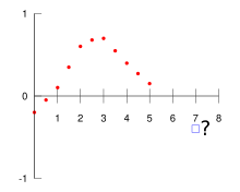
Example illustration of the extrapolation problem, consisting of assigning a meaningful value at the blue box, at  , given the red data points
Methods[edit]
A sound choice of which extrapolation method to apply relies on a priori knowledge of the process that created the existing data points. Some experts have proposed the use of causal forces in the evaluation of extrapolation methods.[2] Crucial questions are, for example, if the data can be assumed to be continuous, smooth, possibly periodic, etc.
Linear[edit]
Linear extrapolation means creating a tangent line at the end of the known data and extending it beyond that limit. Linear extrapolation will only provide good results when used to extend the graph of an approximately linear function or not too far beyond the known data.
If the two data points nearest the point  to be extrapolated are
  and
and  , linear extrapolation gives the function:

(which is identical to linear interpolation if  ). It is possible to include more than two points, and averaging the slope of the linear interpolant, by regression-like techniques, on the data points chosen to be included. This is similar to linear prediction.
Polynomial[edit]

Lagrange extrapolations of the sequence 1,2,3. Extrapolating by 4 leads to a polynomial of minimal degree (cyan line).
A polynomial curve can be created through the entire known data or just near the end (two points for linear extrapolation, three points for quadratic extrapolation, etc.). The resulting curve can then be extended beyond the end of the known data. Polynomial extrapolation is typically done by means of Lagrange interpolation or using Newton’s method of finite differences to create a Newton series that fits the data. The resulting polynomial may be used to extrapolate the data.
High-order polynomial extrapolation must be used with due care. For the example data set and problem in the figure above, anything above order 1 (linear extrapolation) will possibly yield unusable values; an error estimate of the extrapolated value will grow with the degree of the polynomial extrapolation. This is related to Runge’s phenomenon.
Conic[edit]
A conic section can be created using five points near the end of the known data. If the conic section created is an ellipse or circle, when extrapolated it will loop back and rejoin itself. An extrapolated parabola or hyperbola will not rejoin itself, but may curve back relative to the X-axis. This type of extrapolation could be done with a conic sections template (on paper) or with a computer.
French curve[edit]
French curve extrapolation is a method suitable for any distribution that has a tendency to be exponential, but with accelerating or decelerating factors.[3] This method has been used successfully in providing forecast projections of the growth of HIV/AIDS in the UK since 1987 and variant CJD in the UK for a number of years. Another study has shown that extrapolation can produce the same quality of forecasting results as more complex forecasting strategies.[4]
[edit]
Can be created with 3 points of a sequence and the «moment» or «index», this type of extrapolation have 100% accuracy in predictions in a big percentage of known series database (OEIS).[5]
Example of extrapolation with error prediction :
sequence = [1,2,3,5]
f1(x,y) = (x) / y
d1 = f1 (3,2)
d2 = f1 (5,3)
m = last sequence (5)
n = last $ last sequence
fnos (m,n,d1,d2) = round ( ( ( n * d1 ) — m ) + ( m * d2 ) )
round $ ((3*1.66)-5) + (5*1.6) = 8
Quality[edit]
Typically, the quality of a particular method of extrapolation is limited by the assumptions about the function made by the method. If the method assumes the data are smooth, then a non-smooth function will be poorly extrapolated.
In terms of complex time series, some experts have discovered that extrapolation is more accurate when performed through the decomposition of causal forces.[6]
Even for proper assumptions about the function, the extrapolation can diverge severely from the function. The classic example is truncated power series representations of sin(x) and related trigonometric functions. For instance, taking only data from near the x = 0, we may estimate that the function behaves as sin(x) ~ x. In the neighborhood of x = 0, this is an excellent estimate. Away from x = 0 however, the extrapolation moves arbitrarily away from the x-axis while sin(x) remains in the interval [−1, 1]. I.e., the error increases without bound.
Taking more terms in the power series of sin(x) around x = 0 will produce better agreement over a larger interval near x = 0, but will produce extrapolations that eventually diverge away from the x-axis even faster than the linear approximation.
This divergence is a specific property of extrapolation methods and is only circumvented when the functional forms assumed by the extrapolation method (inadvertently or intentionally due to additional information) accurately represent the nature of the function being extrapolated. For particular problems, this additional information may be available, but in the general case, it is impossible to satisfy all possible function behaviors with a workably small set of potential behavior.
In the complex plane[edit]
In complex analysis, a problem of extrapolation may be converted into an interpolation problem by the change of variable  . This transform exchanges the part of the complex plane inside the unit circle with the part of the complex plane outside of the unit circle. In particular, the compactification point at infinity is mapped to the origin and vice versa. Care must be taken with this transform however, since the original function may have had «features», for example poles and other singularities, at infinity that were not evident from the sampled data.
Another problem of extrapolation is loosely related to the problem of analytic continuation, where (typically) a power series representation of a function is expanded at one of its points of convergence to produce a power series with a larger radius of convergence. In effect, a set of data from a small region is used to extrapolate a function onto a larger region.
Again, analytic continuation can be thwarted by function features that were not evident from the initial data.
Also, one may use sequence transformations like Padé approximants and Levin-type sequence transformations as extrapolation methods that lead to a summation of power series that are divergent outside the original radius of convergence. In this case, one often obtains
rational approximants.
Fast[edit]
The extrapolated data often convolute to a kernel function. After data is extrapolated, the size of data is increased N times, here N is approximately 2–3. If this data needs to be convoluted to a known kernel function, the numerical calculations will increase N log(N) times even with fast Fourier transform (FFT). There exists an algorithm, it analytically calculates the contribution from the part of the extrapolated data. The calculation time can be omitted compared with the original convolution calculation. Hence with this algorithm the calculations of a convolution using the extrapolated data is nearly not increased. This is referred as the fast extrapolation. The fast extrapolation has been applied to CT image reconstruction.[7]
[edit]
Extrapolation arguments are informal and unquantified arguments which assert that something is probably true beyond the range of values for which it is known to be true. For example, we believe in the reality of what we see through magnifying glasses because it agrees with what we see with the naked eye but extends beyond it; we believe in what we see through light microscopes because it agrees with what we see through magnifying glasses but extends beyond it; and similarly for electron microscopes. Such arguments are widely used in biology in extrapolating from animal studies to humans and from pilot studies to a broader population.[8]
Like slippery slope arguments, extrapolation arguments may be strong or weak depending on such factors as how far the extrapolation goes beyond the known range.[9]
See also[edit]
- Forecasting
- Minimum polynomial extrapolation
- Multigrid method
- Prediction interval
- Regression analysis
- Richardson extrapolation
- Static analysis
- Trend estimation
- Extrapolation domain analysis
- Dead reckoning
- Interior reconstruction
- Extreme value theory
- Interpolation
Notes[edit]
- ^ Extrapolation, entry at Merriam–Webster
- ^ J. Scott Armstrong; Fred Collopy (1993). «Causal Forces: Structuring Knowledge for Time-series Extrapolation». Journal of Forecasting. 12 (2): 103–115. CiteSeerX 10.1.1.42.40. doi:10.1002/for.3980120205. S2CID 3233162. Retrieved 2012-01-10.
- ^ AIDSCJDUK.info Main Index
- ^ J. Scott Armstrong (1984). «Forecasting by Extrapolation: Conclusions from Twenty-Five Years of Research». Interfaces. 14 (6): 52–66. CiteSeerX 10.1.1.715.6481. doi:10.1287/inte.14.6.52. S2CID 5805521. Retrieved 2012-01-10.
- ^ V. Nos (2021). «Geometric Extrapolation of Integer Sequences».
- ^ J. Scott Armstrong; Fred Collopy; J. Thomas Yokum (2004). «Decomposition by Causal Forces: A Procedure for Forecasting Complex Time Series» (PDF).
- ^ Shuangren Zhao; Kang Yang; Xintie Yang (2011). «Reconstruction from truncated projections using mixed extrapolations of exponential and quadratic functions» (PDF). Journal of X-Ray Science and Technology. 19 (2): 155–72. doi:10.3233/XST-2011-0284. PMID 21606580. Archived from the original (PDF) on 2017-09-29. Retrieved 2014-06-03.
- ^ Steel, Daniel (2007). Across the Boundaries: Extrapolation in Biology and Social Science. Oxford: Oxford University Press. ISBN 9780195331448.
- ^ Franklin, James (2013). «Arguments whose strength depends on continuous variation». Journal of Informal Logic. 33 (1): 33–56. doi:10.22329/il.v33i1.3610. Retrieved 29 June 2021.
References[edit]
- Extrapolation Methods. Theory and Practice by C. Brezinski and M. Redivo Zaglia, North-Holland, 1991.
- Avram Sidi: «Practical Extrapolation Methods: Theory and Applications», Cambridge University Press, ISBN 0-521-66159-5 (2003).
- Claude Brezinski and Michela Redivo-Zaglia : «Extrapolation and Rational Approximation», Springer Nature, Switzerland, ISBN 9783030584177, (2020).
From Wikipedia, the free encyclopedia
In mathematics, extrapolation is a type of estimation, beyond the original observation range, of the value of a variable on the basis of its relationship with another variable. It is similar to interpolation, which produces estimates between known observations, but extrapolation is subject to greater uncertainty and a higher risk of producing meaningless results. Extrapolation may also mean extension of a method, assuming similar methods will be applicable. Extrapolation may also apply to human experience to project, extend, or expand known experience into an area not known or previously experienced so as to arrive at a (usually conjectural) knowledge of the unknown[1] (e.g. a driver extrapolates road conditions beyond his sight while driving). The extrapolation method can be applied in the interior reconstruction problem.
Example illustration of the extrapolation problem, consisting of assigning a meaningful value at the blue box, at , given the red data points
Methods[edit]
A sound choice of which extrapolation method to apply relies on a priori knowledge of the process that created the existing data points. Some experts have proposed the use of causal forces in the evaluation of extrapolation methods.[2] Crucial questions are, for example, if the data can be assumed to be continuous, smooth, possibly periodic, etc.
Linear[edit]
Linear extrapolation means creating a tangent line at the end of the known data and extending it beyond that limit. Linear extrapolation will only provide good results when used to extend the graph of an approximately linear function or not too far beyond the known data.
If the two data points nearest the point to be extrapolated are and , linear extrapolation gives the function:
(which is identical to linear interpolation if ). It is possible to include more than two points, and averaging the slope of the linear interpolant, by regression-like techniques, on the data points chosen to be included. This is similar to linear prediction.
Polynomial[edit]
Lagrange extrapolations of the sequence 1,2,3. Extrapolating by 4 leads to a polynomial of minimal degree (cyan line).
A polynomial curve can be created through the entire known data or just near the end (two points for linear extrapolation, three points for quadratic extrapolation, etc.). The resulting curve can then be extended beyond the end of the known data. Polynomial extrapolation is typically done by means of Lagrange interpolation or using Newton’s method of finite differences to create a Newton series that fits the data. The resulting polynomial may be used to extrapolate the data.
High-order polynomial extrapolation must be used with due care. For the example data set and problem in the figure above, anything above order 1 (linear extrapolation) will possibly yield unusable values; an error estimate of the extrapolated value will grow with the degree of the polynomial extrapolation. This is related to Runge’s phenomenon.
Conic[edit]
A conic section can be created using five points near the end of the known data. If the conic section created is an ellipse or circle, when extrapolated it will loop back and rejoin itself. An extrapolated parabola or hyperbola will not rejoin itself, but may curve back relative to the X-axis. This type of extrapolation could be done with a conic sections template (on paper) or with a computer.
French curve[edit]
French curve extrapolation is a method suitable for any distribution that has a tendency to be exponential, but with accelerating or decelerating factors.[3] This method has been used successfully in providing forecast projections of the growth of HIV/AIDS in the UK since 1987 and variant CJD in the UK for a number of years. Another study has shown that extrapolation can produce the same quality of forecasting results as more complex forecasting strategies.[4]
[edit]
Can be created with 3 points of a sequence and the «moment» or «index», this type of extrapolation have 100% accuracy in predictions in a big percentage of known series database (OEIS).[5]
Example of extrapolation with error prediction :
sequence = [1,2,3,5]
f1(x,y) = (x) / y
d1 = f1 (3,2)
d2 = f1 (5,3)
m = last sequence (5)
n = last $ last sequence
fnos (m,n,d1,d2) = round ( ( ( n * d1 ) — m ) + ( m * d2 ) )
round $ ((3*1.66)-5) + (5*1.6) = 8
Quality[edit]
Typically, the quality of a particular method of extrapolation is limited by the assumptions about the function made by the method. If the method assumes the data are smooth, then a non-smooth function will be poorly extrapolated.
In terms of complex time series, some experts have discovered that extrapolation is more accurate when performed through the decomposition of causal forces.[6]
Even for proper assumptions about the function, the extrapolation can diverge severely from the function. The classic example is truncated power series representations of sin(x) and related trigonometric functions. For instance, taking only data from near the x = 0, we may estimate that the function behaves as sin(x) ~ x. In the neighborhood of x = 0, this is an excellent estimate. Away from x = 0 however, the extrapolation moves arbitrarily away from the x-axis while sin(x) remains in the interval [−1, 1]. I.e., the error increases without bound.
Taking more terms in the power series of sin(x) around x = 0 will produce better agreement over a larger interval near x = 0, but will produce extrapolations that eventually diverge away from the x-axis even faster than the linear approximation.
This divergence is a specific property of extrapolation methods and is only circumvented when the functional forms assumed by the extrapolation method (inadvertently or intentionally due to additional information) accurately represent the nature of the function being extrapolated. For particular problems, this additional information may be available, but in the general case, it is impossible to satisfy all possible function behaviors with a workably small set of potential behavior.
In the complex plane[edit]
In complex analysis, a problem of extrapolation may be converted into an interpolation problem by the change of variable . This transform exchanges the part of the complex plane inside the unit circle with the part of the complex plane outside of the unit circle. In particular, the compactification point at infinity is mapped to the origin and vice versa. Care must be taken with this transform however, since the original function may have had «features», for example poles and other singularities, at infinity that were not evident from the sampled data.
Another problem of extrapolation is loosely related to the problem of analytic continuation, where (typically) a power series representation of a function is expanded at one of its points of convergence to produce a power series with a larger radius of convergence. In effect, a set of data from a small region is used to extrapolate a function onto a larger region.
Again, analytic continuation can be thwarted by function features that were not evident from the initial data.
Also, one may use sequence transformations like Padé approximants and Levin-type sequence transformations as extrapolation methods that lead to a summation of power series that are divergent outside the original radius of convergence. In this case, one often obtains
rational approximants.
Fast[edit]
The extrapolated data often convolute to a kernel function. After data is extrapolated, the size of data is increased N times, here N is approximately 2–3. If this data needs to be convoluted to a known kernel function, the numerical calculations will increase N log(N) times even with fast Fourier transform (FFT). There exists an algorithm, it analytically calculates the contribution from the part of the extrapolated data. The calculation time can be omitted compared with the original convolution calculation. Hence with this algorithm the calculations of a convolution using the extrapolated data is nearly not increased. This is referred as the fast extrapolation. The fast extrapolation has been applied to CT image reconstruction.[7]
[edit]
Extrapolation arguments are informal and unquantified arguments which assert that something is probably true beyond the range of values for which it is known to be true. For example, we believe in the reality of what we see through magnifying glasses because it agrees with what we see with the naked eye but extends beyond it; we believe in what we see through light microscopes because it agrees with what we see through magnifying glasses but extends beyond it; and similarly for electron microscopes. Such arguments are widely used in biology in extrapolating from animal studies to humans and from pilot studies to a broader population.[8]
Like slippery slope arguments, extrapolation arguments may be strong or weak depending on such factors as how far the extrapolation goes beyond the known range.[9]
See also[edit]
- Forecasting
- Minimum polynomial extrapolation
- Multigrid method
- Prediction interval
- Regression analysis
- Richardson extrapolation
- Static analysis
- Trend estimation
- Extrapolation domain analysis
- Dead reckoning
- Interior reconstruction
- Extreme value theory
- Interpolation
Notes[edit]
- ^ Extrapolation, entry at Merriam–Webster
- ^ J. Scott Armstrong; Fred Collopy (1993). «Causal Forces: Structuring Knowledge for Time-series Extrapolation». Journal of Forecasting. 12 (2): 103–115. CiteSeerX 10.1.1.42.40. doi:10.1002/for.3980120205. S2CID 3233162. Retrieved 2012-01-10.
- ^ AIDSCJDUK.info Main Index
- ^ J. Scott Armstrong (1984). «Forecasting by Extrapolation: Conclusions from Twenty-Five Years of Research». Interfaces. 14 (6): 52–66. CiteSeerX 10.1.1.715.6481. doi:10.1287/inte.14.6.52. S2CID 5805521. Retrieved 2012-01-10.
- ^ V. Nos (2021). «Geometric Extrapolation of Integer Sequences».
- ^ J. Scott Armstrong; Fred Collopy; J. Thomas Yokum (2004). «Decomposition by Causal Forces: A Procedure for Forecasting Complex Time Series» (PDF).
- ^ Shuangren Zhao; Kang Yang; Xintie Yang (2011). «Reconstruction from truncated projections using mixed extrapolations of exponential and quadratic functions» (PDF). Journal of X-Ray Science and Technology. 19 (2): 155–72. doi:10.3233/XST-2011-0284. PMID 21606580. Archived from the original (PDF) on 2017-09-29. Retrieved 2014-06-03.
- ^ Steel, Daniel (2007). Across the Boundaries: Extrapolation in Biology and Social Science. Oxford: Oxford University Press. ISBN 9780195331448.
- ^ Franklin, James (2013). «Arguments whose strength depends on continuous variation». Journal of Informal Logic. 33 (1): 33–56. doi:10.22329/il.v33i1.3610. Retrieved 29 June 2021.
References[edit]
- Extrapolation Methods. Theory and Practice by C. Brezinski and M. Redivo Zaglia, North-Holland, 1991.
- Avram Sidi: «Practical Extrapolation Methods: Theory and Applications», Cambridge University Press, ISBN 0-521-66159-5 (2003).
- Claude Brezinski and Michela Redivo-Zaglia : «Extrapolation and Rational Approximation», Springer Nature, Switzerland, ISBN 9783030584177, (2020).
15
МОСКОВСКИЙ ГОСУДАРСТВЕННЫЙ УНИВЕРСИТЕТ им. М.В. ЛОМОНОСОВА
ФАКУЛЬТЕТ ВОЕННОГО ОБУЧЕНИЯ
КАФЕДРА ВОЙСК ПВО
У Т В Е Р Ж Д А Ю
Начальник военной кафедры Войск ПВО
ФВО при МГУ им. М.В. Ломоносова
полковник
И.Я. КАЛАШНИКОВ
“ “ _____________ 199 г.
МЕТОДИЧЕСКАЯ РАЗРАБОТКА
для проведения занятий по военно-специальной
подготовке со студентами, обучающимися по ВУС — 530700
ТЕМА 7. Применение методов статистических решений к задачам
обработки информации.
Занятие 7.2 Завязка и сопровождение траектории цели.
Последовательное сглаживание и оценка параметров
траектории цели.
Обсуждена на методическом заседании цикла №24
протокол №___ от « » ____________ 199 года
МОСКВА — 199 год
Учебные и воспитательные цели
Изучить математический аппарат подалгоритмов завязывания траекторий, стробирования и сопровождения целей. Познакомится с алгоритмом сглаживания, параметров траектории методом последовательного сглаживания. Научится определять точностные характеристики сглаженной траектории. Получить практику в решении задачи сглаживания путем выполнения контрольного задания.
Воспитывать у студентов строевую подтянутость, вырабатывать у них методические и командные навыки.
.
Учебные вопросы:
-
Автозахват траектории цели. Координатные и точностные характеристики захваченной цели.
-
Экстраполяция параметров траектории.
-
Автосопровождение цели.
-
Алгоритм последовательного сглаживания (фильтр Кальмана)
-
Последовательное сглаживание параметров линейной траектории.
Учебное время: 4 часа
МЕТОДИКА ПРОВЕДЕНИЯ ЗАНЯТИЯ
Напомнить студентам о правилах сглаживания траектории и оценки ее параметров. Провести опрос студентов по пройденному занятию (занятие 7.1)
Далее следует рассмотреть вопрос, связанный с этапом захвата и завязывания траекторий. При этом рекомендуется использовать слайды с заранее подготовленными рисунками. Вопрос рассматривается преподавателем.
Рассмотрение вопроса последовательного сглаживания траектории необходимо начать с повторения вопросов теоремы Байеса. Далее с помощью слайдов и работы у доски вывести выражения для уточнения параметров траектории движения цели методом последовательного сглаживания. Представить последовательность действий алгоритма по решению этой задачи. Далее необходимо остановится на особенностях применения данного алгоритма сглаживания. (Вопрос рассматривается преподавателем)
После рассмотрения данного вопроса студенты с помощью преподавателя составляют алгоритм решения задачи сглаживания.
Последним этапом занятия является выполнение контрольного задания. В случае если задание выполнить на занятии удается, ее окончание необходимо дать на самоподготовку.
В ходе занятий обращать внимание на правильность выполнения студентами строевых приемов, а также на последовательность изложения материала при ответах на поставленные вопросы.
В процессе вторичной обработки радиолокационной информации решаются следующие задачи:
-
автозахват и обнаружение траекторий целей,
-
сопровождение траекторий целей,
-
траекторные расчеты.
УЧЕБНЫЙ ВОПРОС 1.
АВТОЗАХВАТ ТРАЕКТОРИИ ЦЕЛИ.
КООРДИНАТНЫЕ И ТОЧНОСТНЫЕ ХАРАКТЕРИСТИКИ ЗАХВАЧЕННОЙ ТРАЕКТОРИИ ЦЕЛИ.
Обнаружение траекторий целей в процессе вторичной обработки обычно осуществляется автоматически. Рассмотрим один из возможных способов автоматического обнаружения траектории цели по данным двухкоординатной РЛС.
Примечание Поскольку в системе обработки РЛИ применяются различные системы координат и различные обозначения, то в дальнейшем, координаты будем обозначать переменными x и y
Пусть появилась одиночная отметка в некоторой точке зоны обзора РЛС.
![]()
![]()
Очевидно эту отметку необходимо принять за первую (начальную) отметку траектории новой цели. Теперь если известны минимальная скорость движения цели ![]() , и максимальная скорость движения цели
, и максимальная скорость движения цели ![]() то область в которой следует искать принадлежащую этой цели вторую отметку в следующем обзоре, можно представить в виде кольца с внутренним и внешним радиусами.
то область в которой следует искать принадлежащую этой цели вторую отметку в следующем обзоре, можно представить в виде кольца с внутренним и внешним радиусами.
![]()
![]() где Т- период обзора
где Т- период обзора
Операция формирования области поиска вторых отметок называется стробированием, а сама область – стробом первичного захвата. В строб захвата может попасть не одна, а несколько отметок
Отметки полученные за второй период обзора.
T- период oбзора
![]()
![]()
![]()
Каждую из них следует считать возможным продолжением предпологаемой траектории. По двум отметкам можно вычислить скорость, направление полета и корреляционную матрицу каждой из предпологаемой траекторий (т.е провести сглаживание). Данная операция называется захвытом траектории.
ПРИМЕЧАНИЕ Если обработка идет в прямоугольной системе координат, то факт попадания второй отметки в строб захвата определяется из условия:
Rmin < ![]() < Rmax где:
< Rmax где: ![]()
![]()
Для каждой из захваченной траектории вычисляется:
Подобные расчеты необходимо провести по каждой захваченной траектории
![]() и
и 
![]() и
и 
Подробнее смотри ПРИМЕЧАНИЕ
Схема захвата траектории

Y
![]()
![]()
![]()
![]()
ПАРАМЕТРЫ
ЗАВЯЗАННЫХ
ТРАЕКТОРИЙ
![]()
![]()
![]()
![]()
X
ПРИМЕЧАНИЕ:
![]()
где
![]()

![]()
Аналогично и для координаты y
УЧЕБНЫЙ Вопрос 2.
Экстраполяция параметров траектории.
2.1 Экстраполяция параметров траектории.
Под экстраполяцией понимают операцию расчета возможного положения отметки на следующий обзор (или на несколько обзоров вперед иди назад). Таким образом, задачей экстраполяции является определение параметров траектории в точке, лежащей вне интервала наблюдения по их значениям внутри этого интервала.
На практике задача экстраполяции решается путем использования сглаженных значений параметров в выбранной точке внутри интервала наблюдения и гипотезе о законе изменения этих параметров вне интервала наблюдения. (Рисунок)
При полиномиальной модели движения цели экстраполированные на время ![]() параметры определяются следующим образом:
параметры определяются следующим образом:

В векторно-матричной форме данное выражение выглядит следующим образом:
![]() ,
,
где ![]() — матричный оператор, записываемый в виде
— матричный оператор, записываемый в виде
 .
.
Тогда выражение для экстраполированных параметров в развернутом виде будет выглядеть так:

-
Экстраполяция ошибок сглаживания.
Ввиду того, что для экстраполяции используются не реальные, а сглаженные значения параметров, то экстраполированные параметры рассчитываются с ошибкой, и поэтому для оценки точности экстраполированных значений необходимо знать ошибки экстраполяции.
Корреляционная матрица ошибок экстраполяции вычисляется следующим образом. Аналогично, как и для экстраполяции параметров, выражение для экстраполяции ошибок записывается в виде:
![]() , где
, где ![]() .
.
По определению корреляционная матрица ошибок экстраполяции равна
![]() ,
,
так как ![]() , то
, то
![]() ,
,
где
![]() .
.
и тогда
![]() .
.
Таким образом, корреляционная матрица ошибок экстраполяции получается путем преобразования матрицы ошибок оценки.
При экстраполяции корреляционной матрицы изменяются значения элементов матрицы. Зависимость элементов матрицы от времени экстраполяции представлены на следующем графике
![]()

![]()
![]()
Рис
Некоторые характеристики сглаженной и экстраполированной точки представлены на графике
y
![]()
![]()
![]()
![]()
![]()
![]()
![]()
x
![]()
![]()
Рис
Итак, результатом экстраполяции на очередном шаге вторичной обработки является:
-
Экстраполированный вектор параметров траектории.
-
Корреляционная матрица ошибок экстраполяции.
УЧЕБНЫЙ Вопрос 3.
Автосопровождение цели.
Постановка задачи
По окончании цикла сглаживания, алгоритм обработки информации ожидает появления новых отметок.
Итак, по результатам очередного обзора получено несколько новых отметок. Возникает задача идентификации, т.е. определения того, к каким уже сопровождаемым траекториям относятся вновь полученные отметки. Эта задача может быть решена путем сравнения координат предполагаемого положения отметки с координатами вновь полученных отметок. Однако объем вычислений при этом будет очень велик.
Для упрощения процесса идентификации и сокращения объема вычислений сравнение координат обычно производится в стробах.
Строб — это область пространства с центром в точке предполагаемого появления отметки.
Центр строба рассчитывается путем экстраполяции сглаженных параметров на время следующего обзора. Вокруг этого центра формируется область, именуемая стробом. Размеры и форма строба обычно выбирается так, чтобы вероятность попадания в него отметки, принадлежащей данной экстраполированной траектории, была близка к единице.
3.1 Стробирование отметок от цели
Под стробированием мы будем понимать формирование предполагаемой области появления новой отметки в виде некоторой совокупности чисел (границ строба). Форму строба, как правило, выбирают простейшей, легко реализуемой.
При обработке информации в прямоугольной системе координат простейший строб задается
Метод для оценка новых данных за пределами известных точек данных
В математике, экстраполяция — это тип оценки значения за пределами исходного диапазона наблюдения. переменной на основе ее связи с другой переменной. Это похоже на интерполяцию, которая производит оценки между известными наблюдениями, но экстраполяция подвержена большей неопределенности и более высокому риску получения бессмысленных результатов. Экстраполяция также может означать расширение метода , если будут применимы аналогичные методы. Экстраполяция может также применяться к человеческому опыту для проецирования, расширения или расширения известного опыта в области, неизвестной или ранее испытанной, чтобы прийти к (обычно предполагаемому) знанию неизвестного (например, водитель экстраполирует дорогу условия за пределами его поля зрения во время вождения). Метод экстраполяции может быть применен в задаче внутренней реконструкции.
Пример иллюстрации проблемы экстраполяции, состоящей из присвоения значимого значения синему прямоугольнику в
x = 7 { displaystyle x = 7}
с учетом красных точек данных.
Содержание
- 1 Методы
- 1.1 Линейный
- 1.2 Полиномиальный
- 1.3 Конический
- 1.4 Французская кривая
- 2 Качество
- 3 В комплексной плоскости
- 4 Быстрый
- 5 Аргументы экстраполяции
- 6 См. Также
- 7 Примечания
- 8 Ссылки
Методы
Правильный выбор того, какой метод экстраполяции применить, зависит от предварительного знания процесса, создавшего существующие данные точки. Некоторые эксперты предложили использовать причинные силы при оценке методов экстраполяции. Ключевыми вопросами являются, например, можно ли предположить, что данные являются непрерывными, гладкими, возможно, периодическими и т. Д.
Линейные
Линейная экстраполяция означает создание касательной линии в конце известных данных и расширяя его за этот предел. Линейная экстраполяция даст хорошие результаты только тогда, когда она используется для расширения графика приблизительно линейной функции или не слишком далеко за пределы известных данных.
Если две точки данных, ближайшие к точке x ∗ { displaystyle x _ {*}}, подлежащие экстраполяции, равны (xk — 1, yk — 1) { Displaystyle (x_ {k-1}, y_ {k-1})}и (xk, yk) { displaystyle (x_ {k}, y_ {k})}, линейная экстраполяция дает функцию:
- y (x ∗) = yk — 1 + x ∗ — xk — 1 xk — xk — 1 (yk — yk — 1). { displaystyle y (x _ {*}) = y_ {k-1} + { frac {x _ {*} — x_ {k-1}} {x_ {k} -x_ {k-1}}} (y_ {k} -y_ {k-1}).}

(что идентично линейной интерполяции, если xk — 1 < x ∗ < x k {displaystyle x_{k-1}). Можно включить более двух точек и усреднить наклон линейного интерполянта с помощью методов регрессии для точек данных, выбранных для включения. Это похоже на линейное предсказание.
Полином
экстраполяции Лагранжа последовательности 1,2,3. Экстраполяция на 4 приводит к полиному минимальной степени (голубая линия).
Полиномиальная кривая может быть построена по всем известным данным или только ближе к концу (две точки для линейной экстраполяции, три точки для квадратичной экстраполяции и т. Д.). Полученная кривая затем может быть расширена за пределы известных данных. Полиномиальная экстраполяция обычно выполняется с помощью интерполяции Лагранжа или с использованием метода конечных разностей Ньютона для создания серии Ньютона, которая соответствует данным. Полученный многочлен можно использовать для экстраполяции данных.
Полиномиальную экстраполяцию высокого порядка следует использовать с должной осторожностью. Для примера набора данных и проблемы на рисунке выше все, что выше порядка 1 (линейная экстраполяция), возможно, даст непригодные для использования значения; оценка ошибки экстраполированного значения будет расти с увеличением степени экстраполяции полинома. Это связано с феноменом Рунге..
Коническое
A сечение конуса может быть создано с использованием пяти точек ближе к концу известных данных. Если созданное коническое сечение представляет собой эллипс или круг, при экстраполяции он зациклится и воссоединится. Экстраполированная парабола или гипербола не соединятся сами с собой, но могут изгибаться назад относительно оси X. Этот тип экстраполяции может быть выполнен с помощью шаблона конических сечений (на бумаге) или с помощью компьютера.
Французская кривая
Экстраполяция французской кривой — это метод, подходящий для любого распределения, которое имеет тенденцию быть экспоненциальным, но с факторами ускорения или замедления. Этот метод успешно использовался для составления прогнозов роста ВИЧ / СПИДа в Великобритании с 1987 года и варианта CJD в Великобритании в течение ряда лет. Другое исследование показало, что экстраполяция может дать такое же качество результатов прогнозирования, как и более сложные стратегии прогнозирования.
Качество
Как правило, качество конкретного метода экстраполяции ограничивается предположениями о функция, выполненная методом. Если метод предполагает, что данные гладкие, то не сглаженная функция будет плохо экстраполирована.
Что касается сложных временных рядов, некоторые эксперты обнаружили, что экстраполяция более точна, если выполняется путем разложения причинных сил.
Даже для правильных предположений о функции экстраполяция может сильно отличаться из функции. Классический пример — усеченные степенные серии представления sin (x) и связанных тригонометрических функций. Например, взяв только данные, близкие к x = 0, мы можем оценить, что функция ведет себя как sin (x) ~ x. В окрестности x = 0 это отличная оценка. Однако вне x = 0 экстраполяция произвольно удаляется от оси x, в то время как sin (x) остается в интервале [-1, 1]. То есть погрешность неограниченно возрастает.
Включение большего количества членов в степенной ряд sin (x) вокруг x = 0 приведет к лучшему согласованию в большем интервале около x = 0, но приведет к экстраполяции, которая в конечном итоге отклонится от оси x еще быстрее чем линейное приближение.
Это расхождение является специфическим свойством методов экстраполяции и обходится только в том случае, если функциональные формы, принимаемые методом экстраполяции (случайно или намеренно из-за дополнительной информации), точно отражают природу экстраполируемой функции. Для конкретных задач эта дополнительная информация может быть доступна, но в общем случае невозможно удовлетворить все возможные варианты поведения функций с работоспособным небольшим набором потенциального поведения.
В комплексной плоскости
В комплексном анализе проблема экстраполяции может быть преобразована в задачу интерполяции путем замены переменной z ^ = 1 / z { displaystyle { hat {z}} = 1 / z}. Это преобразование заменяет часть комплексной плоскости внутри единичной окружности на часть комплексной плоскости вне единичной окружности. В частности, точка компактификации на бесконечности отображается в начало координат и наоборот. Однако с этим преобразованием следует проявлять осторожность, поскольку исходная функция могла иметь «особенности», например, полюса и другие особенности, на бесконечности, которые не были очевидны из выборочных данных.
Другая проблема экстраполяции слабо связана с проблемой аналитического продолжения, где (обычно) степенной серией представлением функции является расширен в одной из своих точек сходимости для получения степенного ряда с большим радиусом сходимости. Фактически, набор данных из небольшой области используется для экстраполяции функции на большую область.
Опять же, аналитическому продолжению могут помешать функции функции, которые не были очевидны из исходных данных.
Кроме того, можно использовать преобразования последовательности, такие как аппроксимации Паде, и в качестве методов экстраполяции, которые приводят к суммированию степенного ряда, которые расходятся за пределами исходного радиуса конвергенции. В этом случае часто получают рациональные аппроксимации.
Быстро
Экстраполированные данные часто свертывают в функцию ядра. После экстраполяции данных размер данных увеличивается в N раз, здесь N составляет примерно 2–3. Если эти данные необходимо преобразовать в известную функцию ядра, численные вычисления увеличатся в N log (N) раз даже при использовании быстрого преобразования Фурье (БПФ). Есть алгоритм, который аналитически рассчитывает вклад части экстраполированных данных. Время вычисления можно опустить по сравнению с исходным вычислением свертки. Следовательно, с помощью этого алгоритма вычисления свертки с использованием экстраполированных данных почти не увеличиваются. Это называется быстрой экстраполяцией. Для реконструкции КТ-изображения была применена быстрая экстраполяция.
Аргументы экстраполяции
Аргументы экстраполяции — это неофициальные и неколичественные аргументы, которые утверждают, что что-то верно за пределами диапазона значений, для которых это известно. правда. Например, мы верим в реальность того, что видим через увеличительное стекло, потому что оно согласуется с тем, что мы видим невооруженным глазом, но выходит за его пределы; мы верим в то, что видим в световые микроскопы, потому что это согласуется с тем, что мы видим через увеличительные стекла, но выходит за рамки этого; и то же самое для электронных микроскопов.
Подобно аргументам скользкого пути, аргументы экстраполяции могут быть сильными или слабыми в зависимости от таких факторов, как то, насколько экстраполяция выходит за пределы известного диапазона.
См. Также
- Прогнозирование
- Экстраполяция минимального полинома
- Многосеточный метод
- Интервал прогноза
- Регрессионный анализ
- Экстраполяция Ричардсона
- Статический анализ
- Оценка тренда
- Анализ области экстраполяции
- Точный расчет
- Внутренняя реконструкция
- Теория экстремальных значений
Примечания
Ссылки
- Методы экстраполяции. Теория и практика К. Брезинского и М. Редиво Загля, Северная Голландия, 1991.