From Wikipedia, the free encyclopedia

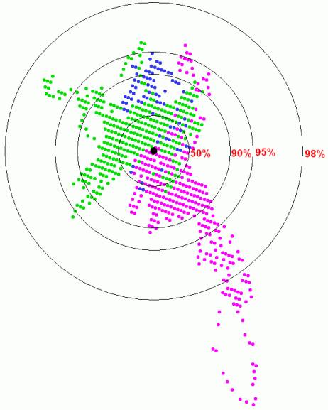
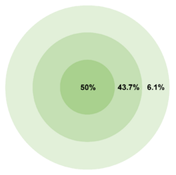
CEP concept and hit probability. 0.2% outside the outmost circle.
In the military science of ballistics, circular error probable (CEP)[1] (also circular error probability[2] or circle of equal probability[3]) is a measure of a weapon system’s precision. It is defined as the radius of a circle, centered on the mean, whose perimeter is expected to include the landing points of 50% of the rounds; said otherwise, it is the median error radius.[4][5] That is, if a given munitions design has a CEP of 100 m, when 100 munitions are targeted at the same point, 50 will fall within a circle with a radius of 100 m around their average impact point. (The distance between the target point and the average impact point is referred to as bias.)
There are associated concepts, such as the DRMS (distance root mean square), which is the square root of the average squared distance error, and R95, which is the radius of the circle where 95% of the values would fall in.
The concept of CEP also plays a role when measuring the accuracy of a position obtained by a navigation system, such as GPS or older systems such as LORAN and Loran-C.
Concept[edit]

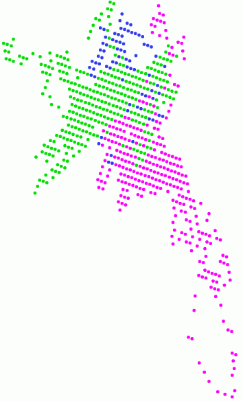
20 hits distribution example
The original concept of CEP was based on a circular bivariate normal distribution (CBN) with CEP as a parameter of the CBN just as μ and σ are parameters of the normal distribution. Munitions with this distribution behavior tend to cluster around the mean impact point, with most reasonably close, progressively fewer and fewer further away, and very few at long distance. That is, if CEP is n metres, 50% of shots land within n metres of the mean impact, 43.7% between n and 2n, and 6.1% between 2n and 3n metres, and the proportion of shots that land farther than three times the CEP from the mean is only 0.2%.
CEP is not a good measure of accuracy when this distribution behavior is not met. Precision-guided munitions generally have more «close misses» and so are not normally distributed. Munitions may also have larger standard deviation of range errors than the standard deviation of azimuth (deflection) errors, resulting in an elliptical confidence region. Munition samples may not be exactly on target, that is, the mean vector will not be (0,0). This is referred to as bias.
To incorporate accuracy into the CEP concept in these conditions, CEP can be defined as the square root of the mean square error (MSE). The MSE will be the sum of the variance of the range error plus the variance of the azimuth error plus the covariance of the range error with the azimuth error plus the square of the bias. Thus the MSE results from pooling all these sources of error, geometrically corresponding to radius of a circle within which 50% of rounds will land.
Several methods have been introduced to estimate CEP from shot data. Included in these methods are the plug-in approach of Blischke and Halpin (1966), the Bayesian approach of Spall and Maryak (1992), and the maximum likelihood approach of Winkler and Bickert (2012). The Spall and Maryak approach applies when the shot data represent a mixture of different projectile characteristics (e.g., shots from multiple munitions types or from multiple locations directed at one target).
Conversion[edit]
While 50% is a very common definition for CEP, the circle dimension can be defined for percentages. Percentiles can be determined by recognizing that the horizontal position error is defined by a 2D vector which components are two orthogonal Gaussian random variables (one for each axis), assumed uncorrelated, each having a standard deviation  . The distance error is the magnitude of that vector; it is a property of 2D Gaussian vectors that the magnitude follows the Rayleigh distribution, with a standard deviation
  , called the distance root mean square (DRMS). In turn, the properties of the Rayleigh distribution are that its percentile at level
 ![{displaystyle Fin [0%,100%]}](https://wikimedia.org/api/rest_v1/media/math/render/svg/9008238d27c0e720af3dcce3bc4b398ac593530d) is given by the following formula:
is given by the following formula:

or, expressed in terms of the DRMS:

The relation between  and
and  are given by the following table, where the values for DRMS and 2DRMS (twice the distance root mean square) are specific to the Rayleigh distribution and are found numerically, while the CEP, R95 (95% radius) and R99.7 (99.7% radius) values are defined based on the 68–95–99.7 rule
| Measure of
|
Probability 
|
|---|---|
| DRMS | 63.213… |
| CEP | 50 |
| 2DRMS | 98.169… |
| R95 | 95 |
| R99.7 | 99.7 |
We can then derive a conversion table to convert values expressed for one percentile level, to another.[6][7] Said conversion table, giving the coefficients  to convert
  into
into  , is given by:
From  to to 
|
RMS ()
|
CEP | DRMS | R95 | 2DRMS | R99.7 |
|---|---|---|---|---|---|---|
| RMS ()
|
1.00 | 1.18 | 1.41 | 2.45 | 2.83 | 3.41 |
| CEP | 0.849 | 1.00 | 1.20 | 2.08 | 2.40 | 2.90 |
| DRMS | 0.707 | 0.833 | 1.00 | 1.73 | 2.00 | 2.41 |
| R95 | 0.409 | 0.481 | 0.578 | 1.00 | 1.16 | 1.39 |
| 2DRMS | 0.354 | 0.416 | 0.500 | 0.865 | 1.00 | 1.21 |
| R99.7 | 0.293 | 0.345 | 0.415 | 0.718 | 0.830 | 1.00 |
For example, a GPS receiver having a 1.25 m DRMS will have a 1.25 m 1.73 = 2.16 m 95% radius.
Warning: often, sensor datasheets or other publications state «RMS» values which in general, but not always,[8] stand for «DRMS» values. Also, be wary of habits coming from properties of a 1D normal distribution, such as the 68-95-99.7 rule, in essence trying to say that «R95 = 2DRMS». As shown above, these properties simply do not translate to the distance errors. Finally, mind that these values are obtained for a theoretical distribution; while generally being true for real data, these may be affected by other effects, which the model does not represent.
See also[edit]
- Probable error
References[edit]
- ^ Circular Error Probable (CEP), Air Force Operational Test and Evaluation Center Technical Paper 6, Ver 2, July 1987, p. 1
- ^ Nelson, William (1988). «Use of Circular Error Probability in Target Detection». Bedford, MA: The MITRE Corporation; United States Air Force. Archived (PDF) from the original on October 28, 2014.
- ^ Ehrlich, Robert (1985). Waging Nuclear Peace: The Technology and Politics of Nuclear Weapons. Albany, NY: State University of New York Press. p. 63.
- ^ Circular Error Probable (CEP), Air Force Operational Test and Evaluation Center Technical Paper 6, ver. 2, July 1987, p. 1
- ^ Payne, Craig, ed. (2006). Principles of Naval Weapon Systems. Annapolis, MD: Naval Institute Press. p. 342.
- ^ Frank van Diggelen, «GPS Accuracy: Lies, Damn Lies, and Statistics», GPS World, Vol 9 No. 1, January 1998
- ^ Frank van Diggelen, «GNSS Accuracy – Lies, Damn Lies and Statistics», GPS World, Vol 18 No. 1, January 2007. Sequel to previous article with similar title [1] [2]
- ^ For instance, the International Hydrographic Organization, in the IHO standard for hydrographic survey S-44 (fifth edition) defines «the 95% confidence level for 2D quantities (e.g. position) is defined as 2.45 x standard deviation», which is true only if we are speaking about the standard deviation of the underlying 1D variable, defined as
 above.
Further reading[edit]
- Blischke, W. R.; Halpin, A. H. (1966). «Asymptotic Properties of Some Estimators of Quantiles of Circular Error». Journal of the American Statistical Association. 61 (315): 618–632. doi:10.1080/01621459.1966.10480893. JSTOR 2282775.
- MacKenzie, Donald A. (1990). Inventing Accuracy: A Historical Sociology of Nuclear Missile Guidance. Cambridge, Massachusetts: MIT Press. ISBN 978-0-262-13258-9.
- Grubbs, F. E. (1964). «Statistical measures of accuracy for riflemen and missile engineers». Ann Arbor, ML: Edwards Brothers. Ballistipedia pdf
- Spall, James C.; Maryak, John L. (1992). «A Feasible Bayesian Estimator of Quantiles for Projectile Accuracy from Non-iid Data». Journal of the American Statistical Association. 87 (419): 676–681. doi:10.1080/01621459.1992.10475269. JSTOR 2290205.
- Daniel Wollschläger (2014), «Analyzing shape, accuracy, and precision of shooting results with shotGroups». Reference manual for shotGroups
- Winkler, V. and Bickert, B. (2012). «Estimation of the circular error probability for a Doppler-Beam-Sharpening-Radar-Mode,» in EUSAR. 9th European Conference on Synthetic Aperture Radar, pp. 368–71, 23/26 April 2012. ieeexplore.ieee.org
External links[edit]
- Circular Error Probable in Ballistipedia
Описание простейшего способа определить точность серии GPS-измерений в заданной точке
[править] Теория
Благодаря некоторым факторам внешней среды влияющим на измерения GPS — в одной и той же точке показания прибора будут разными в разные моменты времени. К таким факторам относится влияние ионосферы, влияние нижних слоев атмосферы, многолучевость, наличие препятствий на пути сигнала и т.д. (Серапинас, 2002).
Показатель CEn — радиус окружности в которую попадает n% локаций (Circular Error), один из простых путей оценить точность производимых GPS измерений в данной точке. Этот показатель является вероятностью того, что определенное измерение будет более точно, чем этот показатель (находится внутри окружности это радиуса).
Показатель CE90 = 10 метров следует читать следующим образом:
- 90% произведенных измерений попали/попадут в окружность радиусом 10 метров, или
- Вероятность того, то новое измерение попало/попадет в окружность радиусом 10 метров равна 90%, или
- 90% произведенных измерений будут точнее 10 метров относительно среднего.
При вычислении окружностей ошибки используется опорная точка, либо задаваемую пользователем, либо вычисляемую как геометрический центр всех измерений, для того, чтобы построить серию окружностей показывающих куда попадает соотвественно определенный процент локаций.
Распространенные названия и значения некоторых показателей:
|
Вероятность |
Название |
|---|---|
|
39.4% |
1 стандартное отклонение |
|
50.0% |
Circular Error Probable (CEP) |
|
63.2% |
Distance RMS (DRMS) |
|
86.5% |
2 стандартных отклонения |
|
95.0% |
95% доверительный интервал |
|
98.2% |
2 DRMS |
|
98.9% |
3 стандартных отклонения |
Показатель точности бытовых приборов чаще всего отражает именно CEP, то есть, приводимые в спецификациях значения, например 15 м, следует понимать так: 50% измерений сделанных данным прибором будут находится в окружности радиусом 15 метров.
[править] Практика
Для того, чтобы определить CEn, необходимо получить серию измерений сделанная в одной точке. Например, включенный и неподвижный GPS с интервалом в 2-5 сек регистрирует точки трека, которые потом загружаются, конвертируются в shape-файл и анализируются.
|
|
Рис. 1 Показания 3-х 40-минутных сессий приема |
Для вычисления CEn может быть использован этот скрипт, данные должны быть спроецированы. При вычислении измеряются расстояния между средней точкой и каждым измерением, а затем считается на каком расстоянии находится нужный процент точек.
|
|
Рис.2 Вычисленные значения CEn в процентах количества локаций (50 — CEP, 90, 95,
50% = 3.42281 |
Пример показывает, что 50% точек находятся на расстоянии 3.4 метра от среднего значения (то есть CEP = 3.4 метра), 98% точек на расстоянии 14.2 метра от среднего. Из диаграммы также виден разброс ошибки.
Для того, чтобы воспроизвести подобный опыт, можно скачать здесь набор готовых данных.
Другими показателями оценки точности GPS являются линейный и сферический показатель вероятности LEP (Linear Error Probable) и SEP (Spherical Error Probable).
[править] Ссылки по теме
- Серапинас Б.Б. Спутниковые системы позиционирования, Москва, 2002 г.
- Error Measures: What does this all mean?
- Linear and Radial and Spherical Error Probabilities
- Ракетная техника
- Словарь РСЗО
- круговое вероятное отклонение
круговое вероятное отклонение
показатель точности попадания (точности стрельбы [1], [7]) реактивных снарядов (бомбы, ракеты, снаряда), применяемый для оценки вероятности поражения цели. Круговое рассеивание является частным случаем более общего понятия вероятного или срединного отклонения, широко используемого в артиллерийской практике и баллистике с XIX века. Как характеристика эффективности ракетного оружия КВО (круговое вероятное отклонение) или по английски CEP (от Circular Error Probable [2], Circular error probable [8], Circular Error of Probability, circular error of probability [3]) введено в оборот в специальной технической литературе в конце 1940-х – начале 1950-х годов.
КВО выражается величиной радиуса круга, очерченного вокруг цели, в который предположительно должно попасть 50 % боеприпасов (или их боевых частей).
В общем случае, если КВО составляет N метров, то 50 % боеприпасов падает на расстояниях от цели меньших либо равных N, 43 % боеприпасов — на расстояниях между N и 2N метров, и 7 % — на расстояниях между 2N и 3N. При нормальном распределении попаданий лишь 0,2 % боеприпасов падает на расстояниях от цели, больших, чем три величины КВО [2].
Показатель кругового вероятного отклонения указывается в метрах или в проценте от дальности стрельбы [4], [5], [6], [7], [8], [9].
Источники:
- Ракетный комплекс «ПОЛОНЕЗ». Рекламный листок BSVT BELSPETSVNESHTECHNIKA. Республика Беларусь. Распространялся на Международном военно-техническом форуме «АРМИЯ-2017» на стенде BSVT BELSPETSVNESHTECHNIKA.
- Круговое вероятное отклонение. [Электронный ресурс] // URL: https://dic.academic.ru/dic.nsf/ruwiki/59790 (дата обращения: 29.04.2020 г.)
- Гуров С.В. Англо-русский и русско-английский словари по реактивным системам залпового огня. – Тула: Гриф и К., 2007 г. – С. 218.
- Гуров С.В. Реактивные системы залпового огня. Обзор. Изд.1, Тула. Издательский дом «Пересвет», 2006 г. – С. 202, 204, 219, 266, 318.
- SR5 220 mm or 122 mm multiple launcher rocket system Norinco — China. [Электронный ресурс]. Дата обновления: 20.06.2012 г. // URL: http://asiandefence-news.blogspot.com/2012/06/sr5-220-mm-or-122-mm-multiple-launcher.html (дата обращения: 31.01.2019 г.)
- Гуров С.В. Реактивная система залпового огня TAKA — 1 (Судан). [Электронный ресурс]. Дата обновления: 16.03.2015 г. // URL: https://missilery.info/gallery/reaktivnaya-sistema-zalpovogo-ognya-taka-1-sudan (дата обращения: 29.04.2020 г.)
- Robin Hughes. Roketsan unveils new 122 mm guided artillery missile. [Электронный ресурс]. Дата обновления: 16.09.2016 г. // URL: http://www.janes.com/article/63844/roketsan-unveils-new-122-mm-guided-artillery-missile (дата обращения: 16.09.2016 г.)
- «Нептун» и «Ольха» в Эмиратах. [Электронный ресурс]. Дата обновления: 17.02.2019 г. // URL: https://andrei-bt.livejournal.com/1120637.html (дата обращения: 18.02.2019 г.)
- Гуров С.В. Опытная реактивная пусковая установка RAP-14. [Электронный ресурс] // URL: https://missilery.info/missile/wobb/rap-14/rap-14.shtml (дата обращения: 29.04.2020 г.)
Автор: С.В. Гуров (Россия, г.Тула)
Данный раздел является частью Энциклопедического иллюстрированного словаря по реактивным системам залпового огня (РСЗО).
Редакторский коллектив (АО «НПО «СПЛАВ», Россия, г.Тула):
- Гуров С.В.
- Самойлова А.В.
- Королёв В.В.
Консультации профильных специалистов (АО «НПО «СПЛАВ», Россия, г.Тула):
- Грибкова Л.П.
- Орлова С.М. (к.т.н.)
- Дмитриев В.Ф. (д.т.н.)
Среднеквадратический эллипс ошибок, круговая вероятная ошибка
Проанализируем
более подробно характеристики,
используемые для описания свойств
двухмерных гауссовских векторов.
Двухмерный случай весьма важен в задачах
обработки статистической информации.
Так, при решении навигационных задач
на плоскости нередко полагают, что
координаты объекта представляют собой
гауссовский случайный вектор с
математическим ожиданием в точке его
предполагаемого местонахождения. Для
описания неопределенности расположения
точки на плоскости используют введенные
выше эллипсы равных вероятностей, в
частности эллипс, соответствующий
уравнению (3.35) при
![]() .
.
Поскольку этот эллипс пересекает оси
в точках, совпадающих со значениями
соответствующих СКО, т.е. при![]() ,
,
а при![]()
![]() ,
,
он получил наименованиесреднеквадратического
эллипса ошибок, или стандартного эллипса
[23]. В
навигационных приложениях для его
описания используют параметры
эллипса:
большую
![]() ималую
ималую
![]() полуоси
полуоси
и дирекционный
угол
![]() ,
,
задающий ориентацию большой полуоси
относительно оси![]() .
.
Эти три параметра полностью определяют
матрицу ковариаций двухмерной гауссовской
плотности. На рис. 3.4 изображен частный
случай, когда![]() ,
,
![]() ,
,
![]() ,
,
и таким
образом
![]() , (3.36)
, (3.36)
т.е. размеры полуосей
эллипса определяют значения СКО по
каждой координате.
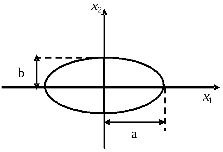
Рис.
1.2.4. Эллипс ошибок для двухмерного
гауссовского вектора
с независимыми
компонентами
При оценивании
точности местоположения подвижных
объектов весьма важным представляется
умение охарактеризовать неопределенность
местоположения одним
числом. Для
этих целей обычно используют значения
вероятности
попадания
точки на плоскости в ту или иную заданную
область
![]() .
.
Для двухмерного центрированного
гауссовского вектора с плотностью
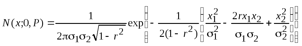
эта вероятность
определяется как
 , (3.37)
Если в качестве
![]() выступает область, ограниченная
выступает область, ограниченная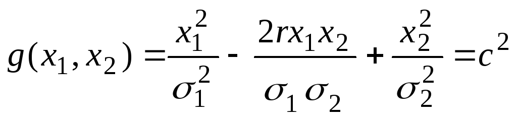
то, переходя к
полярным координатам, можно показать,
что [44, с. 68]
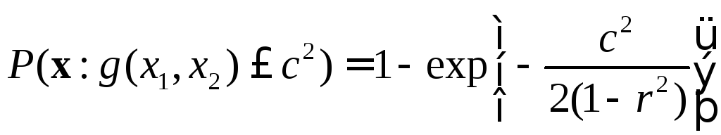 . (3.38)
Для случая
независимых случайных величин при
![]() эллипс превращается в окружность
эллипс превращается в окружность
радиусом![]() и, таким образом, из (3.38) получаем, что
и, таким образом, из (3.38) получаем, что
вероятность нахождения случайного
вектора в круге с таким радиусом
определяется введенным в разделе 2
распределением Рэлея
 ,
,
R>0. (1.39)
Круговая вероятная
ошибка (КВО).
Величина
![]() ,
,
соответствующая 50-процентному попаданию
гауссовского случайного вектора в круг
заданного радиуса, т.е. когда вероятность
попадания равна 0,5, называетсякруговой
вероятной ошибкой (КВО),
а круг, соответственно, кругом
равных вероятностей.
В англоязычной литературе для круговой
вероятной ошибки используется термин
circular error
probable (CEP).
Отметим, что для
независимых
случайных величин с равными
СКО
![]() ,
,
50-процентное попадание в круг (P=0,5)
достигается при
![]() 1,177.
1,177.
Для круга радиуса
![]() обеспечивается попадание с вероятностьюP=0,997.
обеспечивается попадание с вероятностьюP=0,997.
В случае если
![]() радиус круга, при котором достигается
радиус круга, при котором достигается
вероятность попадания в него, равная
0,5, либо другой вероятности следует
отыскивать с помощью соотношения (3.37).
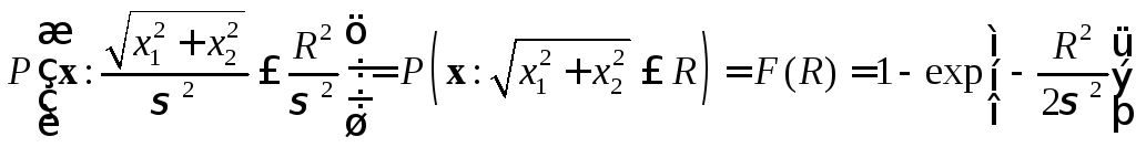
Радиальная
среднеквадратическая ошибка (Distance
Root Mean Square (DRMS)
Эта ошибка
определяется как
![]() . (3.40)
. (3.40)
Отметим, что
вероятность попадания в круг такого
радиуса составляет величину 0.65-0.68 в
зависимости от значений параметров
эллипса рассеивания.
Удвоенная
радиальная среднеквадратическая ошибка
(2DRMS).
Вероятность
попадания в круг такого удвоенного
радиуса зависит от конкретных соотношений
СКО и коэффициента корреляции, а примерная
ее величина определяется как P=0,95.
Понятия, аналогичные
приведенным выше, используются и для
трехмерного гауссовского вектора. При
этом вводится величина сферической
вероятной ошибки (СВО)
и сферы равных
вероятностей
(spherical error
probable (SEP)
и sphere of equal
probability (SEP)). Трехмерное
гауссовское распределение широко
используется при описании ошибок
местоположения подвижных объектов в
пространстве, в частности для летательных
аппаратов.
Соседние файлы в папке Кафедра ТВ
- #
- #
- #
- #
- #
- #
Previous: Precision Models
Contents
- 1 Circular Error Probable (CEP)
- 1.1 Systematic Accuracy Bias
- 1.2 Estimators
- 2 Comparing CEP estimators
- 2.1 Small Samples
- 3 References
Circular Error Probable (CEP)
The Circular Error Probable (CEP(p)) for (p in [0,1)) is the estimated radius of the smallest circle that is expected to cover proportion (p) of the shot group. Some authors restrict the name «CEP» to the case of (p = 0.5), and refer to, e.g., (R95) for (p = 0.95). We make no such distinction here.
How (CEP(p)) should be estimated depends on what assumptions are made regarding the distribution of radial errors, i.e., the distribution of miss distances of shots to the point of aim (POA). In turn, the distribution of radial error depends on the bivariate distribution of x— and y-coordinates of the shots. If the x— and y-coordinates of the shots follow a bivariate normal distribution, the radial error around the POA can follow one of several distributions, depending on the cirumstances (Beckmann 1962; 1964):
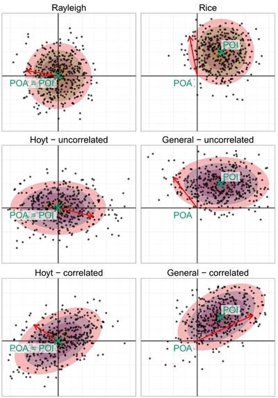
Distribution of radial error (red arrow) in different kinds of bivariate normal distribution. POA = point of aim, POI = mean point of impact
- Rayleigh: When the true center of the coordinates and the POA coincide, the radial error around the POA in a bivariate uncorrelated normal random variable with equal variances follows a Rayleigh distribution. This distribution is described in the Closed Form Precision section. In three dimensions (spherical error probable, SEP), the radial error follows a Maxwell-Boltzmann distribution.
- Rice: When the true center of the coordinates and the POA are not identical, the radial error around the POA in a bivariate uncorrelated normal random variable with equal variances follows a Rice distribution. The probability density function, the cumulative distribution function, and the quantile function are defined in closed form. The Rice distribution reduces to the Rayleigh distribution if the mean coincides with the POA.
- Hoyt: When the true center of the coordinates and the POA coincide, the radius around the POA in a bivariate correlated normal random variable with unequal variances follows a Hoyt distribution. The probability density function and the cumulative distribution function are defined in closed form, whereas numerical methods are required to find the quantile function. The Hoyt distribution reduces to the Rayleigh distribution if the correlation is 0 and the variances are equal.
- The general case obtains if the true center of the coordinates and the POA are not identical, and the shots have a bivariate correlated normal distribution with unequal variances. The cumulative distribution function of radial error is equal to the integral of the bivariate normal distribution over an offset disc. Numerical methods are required to evaluate the distribution. The resulting distribution reduces to the Rice distribution if the correlation is 0 and the variances are equal. The resulting distribution reduces to the Hoyt distribution if the mean has no offset.
Systematic Accuracy Bias
Some approaches to estimating CEP conflate the question of precision with the question of accuracy, or «sighting in.»
The simpler case only tries to estimate precision, and computes CEP about the sample center.
The general case allows that the point-of-aim is offset from the true center point-of-impact. In the literature this is referred to as systematic accuracy bias. Including systematic accuracy bias sets the center of the circle to the point of aim, which means the sample center will probably be offset from that and CEP will be correspondingly larger.
Estimators
Several different methods for estimating (CEP(p)) have been proposed which are based on the different assumptions about the underlying distribution of coordinates outlined above. See the CEP literature overview for references and the shotGroups package for a free open source implementation:
- The general correlated normal estimator (DiDonato & Jarnagin, 1961a; Evans, 1985) is based on the assumption of bivariate normality of the shot coordinates. It allows the x— and y-coordinates to be correlated and have different variances.
- Without taking systematic bias into account, this estimate can be based on the closed-form solution for the Hoyt distribution of radial error (Hoyt, 1947; Paris, 2009). The Krempasky (2003) estimate is based on a nearly correct closed-form solution for the 50% quantile of the Hoyt distribution. The Ignani (2010) estimate is based on a polynomial approximation for the 50%, 90%, 95%, and 99% quantiles of the Hoyt distribution.
- The modified RAND R-234 estimator (Pesapane & Irvine, 1977) is an early example of CEP and is based on lookup tables for the 50% quantile of the Hoyt distribution. The tables were later cast into an algebraic form that is essentially the Rayleigh estimator with a weighted average of the variances of the de-correlated data to estimate the true standard deviation. It works best for a mostly circular distribution of ((x,y))-coordinates (aspect ratio of data ellipse (leq 3)).
- The Valstar estimate (Puhek, 1992) for the 50% quantile of the Hoyt distribution differs from the RAND-estimate only for highly elliptical distributions. This estimate does not generalize to three dimensions.
- Other old, and less relevant approximations to the 50% quantile of the Hoyt distribution include Bell (1973), Nicholson (1974) and Siouris (1993).
- If systematic accuracy bias is taken into account, numerical integration of the multivariate normal distribution around an offset circle is required for an exact solution. The calculation of the correlated normal estimator is difficult and requires numerical approaches only available in specialized software.
- An approximation for the 50% and 90% quantile when there is systematic bias comes from Shultz (1963), later modified by Ager (2004). The RAND-tables have also been fitted with a regression model to accommodate systematic accuracy bias in the 50% quantile (Pesapane & Irvine, 1977). The Valstar estimate (Puhek, 1992) is similar but differs in its method of correcting for systematic accuracy bias.
- The Grubbs-Pearson estimator (Grubbs, 1964) shares its assumptions with the general correlated normal estimator. It is based on the Pearson three-moment central (chi^{2})-approximation (Imhof, 1961; Pearson, 1959) of the cumulative distribution function of radial error in bivariate normal variables. This approach has the advantage that its calculation is much easier than the exact distribution and does not require special software. For (p geq 0.25), the approximation to the true cumulative distribution function is very close but can diverge from it for (p < 0.25) with some distribution shapes.
- The Grubbs-Patnaik estimator (Grubbs, 1964) differs from the Grubbs-Pearson estimator insofar as it is based on the Patnaik two-moment central (chi^{2})-approximation (Patnaik, 1949) of the true cumulative distribution function of radial error. For (p < 0.5) with some distribution shapes, the approximation can diverge significantly from the true cumulative distribution function.
- The Grubbs-Liu estimate was not proposed by Grubbs but can be constructed following the same principle as his original estimators. It differs from them insofar as it is based on the recent Liu, Tang, and Zhang (2009) four-moment non-central (chi^{2})-approximation of the true cumulative distribution function of radial error.
- The Rayleigh estimator uses the Rayleigh quantile function for radial error (Culpepper, 1978; Singh, 1992). It assumes an uncorrelated bivariate normal process with equal variances and zero mean. Note that this estimator is essentially the same as the RMSE estimator often described in the GPS literature when using centered data for calculating MSE.[1] [2][3] The only difference is that RMSE uses a biased estimate of the true standard deviation.
- If systematic accuracy bias is taken into account, this estimator becomes the Rice estimator. Note that for small bias, this estimator is similar to the RMSE estimator often described in the GPS literature when using the original, non-centered data for calculating MSE. With large bias however, the RMSE estimator becomes seriously wrong.
- The Ethridge (1983) estimator is not based on the assumption of bivariate normality of ((x,y))-coordinates but uses a robust unbiased estimator for the median radius (Hogg, 1967). This estimator «assumes that the square root of the radial miss distances follows the logarithmic generalized exponential power distribution.» (Williams, 1997). It is only available for (p = 0.5).
Comparing CEP estimators
If the true variances of x— and y-coordinates as well as their covariance is known then the closed-form general correlated normal estimator is ideal.
When we are confident in asserting a bivariate normal model for shot dispersion the Grubbs estimators are excellent approximations for reasonable values of p and ellipticity.
- To date most comparison studies have only used the Grubbs-Patnaik estimator.
- The Grubbs-Pearson estimator has the theoretical advantage over the Grubbs-Patnaik estimator that the approximating distribution matches the true distribution not only in mean and variance but also in skewness. Both the Grubbs-Pearson and Grubbs-Patnaik estimators are easy to calculate with standard software as long as the central (chi^{2})-distribution is available (as it is, for example, in spreadsheets).
- If systematic accuracy bias is taken into account, the Grubbs-Liu estimator has the theoretical advantage over the Grubbs-Pearson estimator that the approximating distribution matches the true distribution not only in mean, variance, and skewness but also in kurtosis. If systematic accuracy bias is ignored, the Grubbs-Liu estimator is equivalent to the Grubbs-Pearson estimator. Its calculation is less complicated than the exact correlated normal estimator but requires the non-central (chi^{2})-distribution. This distribution might not be available in general tools like spreadsheets, but it is implemented in all statistics packages.
One shortcoming of the Grubbs estimators is that it is not possible to incorporate the confidence intervals of the variance estimates into the CEP estimate. This is particularly relevant to small samples where the variance estimates themselves are subject to considerable error.
In the special case where we assume uncorrelated bivariate normal data with equal variances the Rayleigh estimator does provide true confidence intervals, and it is easy to calculate using spreadsheets.
The Ethridge estimator stands out because it does not require bivariate normality of the ((x,y))-coordinates. It generalizes to three-dimensional data and can accommodate systematic accuracy bias, but it is limited to the 50% CEP.
Small Samples
For small samples we are more sensitive to which estimator is least bias and most efficient. This question has been studied, e.g., by Williams (1997).
A related question is which estimator is most robust to a very small number of outliers (or Fliers) that may result from clear operator error. See the literature overview for more comparison studies.
References
- ↑ GPS Accuracy: Lies, Damn Lies, and Statistics, Frank van Diggelen, GPS World, 1998
- ↑ Update: GNSS Accuracy: Lies, Damn Lies, and Statistics, Frank van Diggelen, GPS World, 2007
- ↑ The Mathematics of GPS, Richard B Langley, GPS World, 1991
In the military science of ballistics, circular error probable (CEP) (also circular error probability or circle of equal probability[1]) is an intuitive measure of a weapon system’s precision. It is defined as the radius of a circle, centered about the mean, whose boundary is expected to include the landing points of 50% of the rounds.[2]
Concept
The original concept of CEP was based on a circular bivariate normal distribution (CBN) with CEP as a parameter of the CBN just as μ and σ are parameters of the normal distribution. Munitions with this distribution behavior tend to cluster around the aim point, with most reasonably close, progressively fewer and fewer further away, and very few at long distance. That is, if CEP is n meters, 50% of rounds land within n meters of the target, 43% between n and 2n, and 7% between 2n and 3n meters, and the proportion of rounds that land farther than three times the CEP from the target is less than 0.2%.
This distribution behavior is often not met. Precision-guided munitions generally have more «close misses» and so are not normally distributed. Munitions may also have larger standard deviation of range errors than the standard deviation of azimuth (deflection) errors, resulting in an elliptical confidence region. Munition samples may not be exactly on target, that is, the mean vector will not be (0,0). This is referred to as bias.
To apply the CEP concept in these conditions, CEP can be defined as the square root of the mean square error (MSE). The MSE will be the sum of the variance of the range error plus the variance of the azimuth error plus the covariance of the range error with the azimuth error plus the square of the bias. Thus the MSE results from pooling all these sources of error, geometrically corresponding to radius of a circle within which 50% of rounds will land.
Conversion between CEP, RMS, 2DRMS, and R95
While 50% is a very common definition for CEP, the circle dimension can be defined for percentages. Approximate formulae are available to convert the distributions along the two axes into the equivalent circle radius for the specified percentage.[3][4]
| Accuracy Measure | Probability (%) |
|---|---|
| Root mean square (RMS) | 63 to 68 |
| Circular error probability (CEP) | 50 |
| Twice the distance root mean square (2DRMS) | 95 to 98 |
| 95% radius (R95) | 95 |
| From/to | CEP | RMS | R95 | 2DRMS |
|---|---|---|---|---|
| CEP | — | 1.2 | 2.1 | 2.4 |
| RMS | 0.83 | — | 1.7 | 2.0 |
| R95 | 0.48 | 0.59 | — | 1.2 |
| 2DRMS | 0.42 | 0.5 | 0.83 | — |
References
- ↑ http://web.archive.org/web/20110720122829/http://www.naval-technology.com/projects/vanguard/
- ↑ Circular Error Probable (CEP), Air Force Operational Test and Evaluation Center Technical Paper 6, Ver 2, July 1987, p. 1
- ↑ «GPS Accuracy: Lies, Damn Lies, and Statistics», GPS World, Vol 9 No. 1, January 1998 [1]
- ↑ “GNSS Accuracy – Lies, Damn Lies and Statistics”, GPS World, Vol 18 No. 1, January 2007. Sequel to previous article with similar title [2]

CEP concept and hit probability. 0.2% outside the outmost circle.
In the military science of ballistics, circular error probable (CEP)[1] (also circular error probability[2] or circle of equal probability[3]) is a measure of a weapon system’s precision. It is defined as the radius of a circle, centered on the mean, whose perimeter is expected to include the landing points of 50% of the rounds; said otherwise, it is the median error radius.[4][5] That is, if a given munitions design has a CEP of 100 m, when 100 munitions are targeted at the same point, 50 will fall within a circle with a radius of 100 m around their average impact point. (The distance between the target point and the average impact point is referred to as bias.)
There are associated concepts, such as the DRMS (distance root mean square), which is the square root of the average squared distance error, and R95, which is the radius of the circle where 95% of the values would fall in.
The concept of CEP also plays a role when measuring the accuracy of a position obtained by a navigation system, such as GPS or older systems such as LORAN and Loran-C.
Concept

20 hits distribution example
The original concept of CEP was based on a circular bivariate normal distribution (CBN) with CEP as a parameter of the CBN just as μ and σ are parameters of the normal distribution. Munitions with this distribution behavior tend to cluster around the mean impact point, with most reasonably close, progressively fewer and fewer further away, and very few at long distance. That is, if CEP is n metres, 50% of shots land within n metres of the mean impact, 43.7% between n and 2n, and 6.1% between 2n and 3n metres, and the proportion of shots that land farther than three times the CEP from the mean is only 0.2%.
CEP is not a good measure of accuracy when this distribution behavior is not met. Precision-guided munitions generally have more «close misses» and so are not normally distributed. Munitions may also have larger standard deviation of range errors than the standard deviation of azimuth (deflection) errors, resulting in an elliptical confidence region. Munition samples may not be exactly on target, that is, the mean vector will not be (0,0). This is referred to as bias.
To incorporate accuracy into the CEP concept in these conditions, CEP can be defined as the square root of the mean square error (MSE). The MSE will be the sum of the variance of the range error plus the variance of the azimuth error plus the covariance of the range error with the azimuth error plus the square of the bias. Thus the MSE results from pooling all these sources of error, geometrically corresponding to radius of a circle within which 50% of rounds will land.
Several methods have been introduced to estimate CEP from shot data. Included in these methods are the plug-in approach of Blischke and Halpin (1966), the Bayesian approach of Spall and Maryak (1992), and the maximum likelihood approach of Winkler and Bickert (2012). The Spall and Maryak approach applies when the shot data represent a mixture of different projectile characteristics (e.g., shots from multiple munitions types or from multiple locations directed at one target).
Conversion
While 50% is a very common definition for CEP, the circle dimension can be defined for percentages. Percentiles can be determined by recognizing that the horizontal position error is defined by a 2D vector which components are two orthogonal Gaussian random variables (one for each axis), assumed uncorrelated, each having a standard deviation . The distance error is the magnitude of that vector; it is a property of 2D Gaussian vectors that the magnitude follows the Rayleigh distribution, with a standard deviation , called the distance root mean square (DRMS). In turn, the properties of the Rayleigh distribution are that its percentile at level is given by the following formula:
or, expressed in terms of the DRMS:
The relation between and are given by the following table, where the values for DRMS and 2DRMS (twice the distance root mean square) are specific to the Rayleigh distribution and are found numerically, while the CEP, R95 (95% radius) and R99.7 (99.7% radius) values are defined based on the 68–95–99.7 rule
| Measure of
|
Probability
|
|---|---|
| DRMS | 63.213… |
| CEP | 50 |
| 2DRMS | 98.169… |
| R95 | 95 |
| R99.7 | 99.7 |
We can then derive a conversion table to convert values expressed for one percentile level, to another.[6][7] Said conversion table, giving the coefficients to convert into , is given by:
| From to
|
RMS ()
|
CEP | DRMS | R95 | 2DRMS | R99.7 |
|---|---|---|---|---|---|---|
| RMS ()
|
1.00 | 1.18 | 1.41 | 2.45 | 2.83 | 3.41 |
| CEP | 0.849 | 1.00 | 1.20 | 2.08 | 2.40 | 2.90 |
| DRMS | 0.707 | 0.833 | 1.00 | 1.73 | 2.00 | 2.41 |
| R95 | 0.409 | 0.481 | 0.578 | 1.00 | 1.16 | 1.39 |
| 2DRMS | 0.354 | 0.416 | 0.500 | 0.865 | 1.00 | 1.21 |
| R99.7 | 0.293 | 0.345 | 0.415 | 0.718 | 0.830 | 1.00 |
For example, a GPS receiver having a 1.25 m DRMS will have a 1.25 m1.73 = 2.16 m 95% radius.
Warning: often, sensor datasheets or other publications state «RMS» values which in general, but not always,[8] stand for «DRMS» values. Also, be wary of habits coming from properties of a 1D normal distribution, such as the 68-95-99.7 rule, in essence trying to say that «R95 = 2DRMS». As shown above, these properties simply do not translate to the distance errors. Finally, mind that these values are obtained for a theoretical distribution; while generally being true for real data, these may be affected by other effects, which the model does not represent.
See also
- Probable error
References
- ^ Circular Error Probable (CEP), Air Force Operational Test and Evaluation Center Technical Paper 6, Ver 2, July 1987, p. 1
- ^ Nelson, William (1988). «Use of Circular Error Probability in Target Detection». Bedford, MA: The MITRE Corporation; United States Air Force. Archived (PDF) from the original on October 28, 2014.
- ^ Ehrlich, Robert (1985). Waging Nuclear Peace: The Technology and Politics of Nuclear Weapons. Albany, NY: State University of New York Press. p. 63.
- ^ Circular Error Probable (CEP), Air Force Operational Test and Evaluation Center Technical Paper 6, ver. 2, July 1987, p. 1
- ^ Payne, Craig, ed. (2006). Principles of Naval Weapon Systems. Annapolis, MD: Naval Institute Press. p. 342.
- ^ Frank van Diggelen, «GPS Accuracy: Lies, Damn Lies, and Statistics», GPS World, Vol 9 No. 1, January 1998
- ^ Frank van Diggelen, «GNSS Accuracy – Lies, Damn Lies and Statistics», GPS World, Vol 18 No. 1, January 2007. Sequel to previous article with similar title [1] [2]
- ^ For instance, the International Hydrographic Organization, in the IHO standard for hydrographic survey S-44 (fifth edition) defines «the 95% confidence level for 2D quantities (e.g. position) is defined as 2.45 x standard deviation», which is true only if we are speaking about the standard deviation of the underlying 1D variable, defined as above.
Further reading
- Blischke, W. R.; Halpin, A. H. (1966). «Asymptotic Properties of Some Estimators of Quantiles of Circular Error». Journal of the American Statistical Association. 61 (315): 618–632. doi:10.1080/01621459.1966.10480893. JSTOR 2282775.
- MacKenzie, Donald A. (1990). Inventing Accuracy: A Historical Sociology of Nuclear Missile Guidance. Cambridge, Massachusetts: MIT Press. ISBN 978-0-262-13258-9.
- Grubbs, F. E. (1964). «Statistical measures of accuracy for riflemen and missile engineers». Ann Arbor, ML: Edwards Brothers. Ballistipedia pdf
- Spall, James C.; Maryak, John L. (1992). «A Feasible Bayesian Estimator of Quantiles for Projectile Accuracy from Non-iid Data». Journal of the American Statistical Association. 87 (419): 676–681. doi:10.1080/01621459.1992.10475269. JSTOR 2290205.
- Daniel Wollschläger (2014), «Analyzing shape, accuracy, and precision of shooting results with shotGroups». Reference manual for shotGroups
- Winkler, V. and Bickert, B. (2012). «Estimation of the circular error probability for a Doppler-Beam-Sharpening-Radar-Mode,» in EUSAR. 9th European Conference on Synthetic Aperture Radar, pp. 368–71, 23/26 April 2012. ieeexplore.ieee.org
External links
- Circular Error Probable in Ballistipedia
![]()
This page was last edited on 4 August 2022, at 14:08
From HandWiki
: Ballistics measure of a weapon system’s precision
CEP concept and hit probability. 0.2% outside the outmost circle.
In the military science of ballistics, circular error probable (CEP)[1] (also circular error probability[2] or circle of equal probability[3]) is a measure of a weapon system’s precision. It is defined as the radius of a circle, centered on the mean, whose perimeter is expected to include the landing points of 50% of the rounds; said otherwise, it is the median error radius.[4][5] That is, if a given munitions design has a CEP of 100 m, when 100 munitions are targeted at the same point, 50 will fall within a circle with a radius of 100 m around their average impact point. (The distance between the target point and the average impact point is referred to as bias.)
There are associated concepts, such as the DRMS (distance root mean square), which is the square root of the average squared distance error, and R95, which is the radius of the circle where 95% of the values would fall in.
The concept of CEP also plays a role when measuring the accuracy of a position obtained by a navigation system, such as GPS or older systems such as LORAN and Loran-C.
Concept

20 hits distribution example
The original concept of CEP was based on a circular bivariate normal distribution (CBN) with CEP as a parameter of the CBN just as μ and σ are parameters of the normal distribution. Munitions with this distribution behavior tend to cluster around the mean impact point, with most reasonably close, progressively fewer and fewer further away, and very few at long distance. That is, if CEP is n metres, 50% of shots land within n metres of the mean impact, 43.7% between n and 2n, and 6.1% between 2n and 3n metres, and the proportion of shots that land farther than three times the CEP from the mean is only 0.2%.
CEP is not a good measure of accuracy when this distribution behavior is not met. Precision-guided munitions generally have more «close misses» and so are not normally distributed. Munitions may also have larger standard deviation of range errors than the standard deviation of azimuth (deflection) errors, resulting in an elliptical confidence region. Munition samples may not be exactly on target, that is, the mean vector will not be (0,0). This is referred to as bias.
To incorporate accuracy into the CEP concept in these conditions, CEP can be defined as the square root of the mean square error (MSE). The MSE will be the sum of the variance of the range error plus the variance of the azimuth error plus the covariance of the range error with the azimuth error plus the square of the bias. Thus the MSE results from pooling all these sources of error, geometrically corresponding to radius of a circle within which 50% of rounds will land.
Several methods have been introduced to estimate CEP from shot data. Included in these methods are the plug-in approach of Blischke and Halpin (1966), the Bayesian approach of Spall and Maryak (1992), and the maximum likelihood approach of Winkler and Bickert (2012). The Spall and Maryak approach applies when the shot data represent a mixture of different projectile characteristics (e.g., shots from multiple munitions types or from multiple locations directed at one target).
Conversion
While 50% is a very common definition for CEP, the circle dimension can be defined for percentages. Percentiles can be determined by recognizing that the horizontal position error is defined by a 2D vector which components are two orthogonal Gaussian random variables (one for each axis), assumed uncorrelated, each having a standard deviation [math]displaystyle{ sigma }[/math]. The distance error is the magnitude of that vector; it is a property of 2D Gaussian vectors that the magnitude follows the Rayleigh distribution, with a standard deviation [math]displaystyle{ sigma_d=sqrt{2}sigma }[/math], called the distance root mean square (DRMS). In turn, the properties of the Rayleigh distribution are that its percentile at level [math]displaystyle{ Fin[0%,100%] }[/math] is given by the following formula:
- [math]displaystyle{ Q(F,sigma)=sigma sqrt{-2ln(1-F/100)} }[/math]
or, expressed in terms of the DRMS:
- [math]displaystyle{ Q(F,sigma_d)=sigma_d frac{sqrt{-2ln(1-F/100)}}{sqrt{2}} }[/math]
The relation between [math]displaystyle{ Q }[/math] and [math]displaystyle{ F }[/math] are given by the following table, where the [math]displaystyle{ F }[/math] values for DRMS and 2DRMS (twice the distance root mean square) are specific to the Rayleigh distribution and are found numerically, while the CEP, R95 (95% radius) and R99.7 (99.7% radius) values are defined based on the 68–95–99.7 rule
| Measure of [math]displaystyle{ Q }[/math] | Probability [math]displaystyle{ F , (%) }[/math] |
|---|---|
| DRMS | 63.213… |
| CEP | 50 |
| 2DRMS | 98.169… |
| R95 | 95 |
| R99.7 | 99.7 |
We can then derive a conversion table to convert values expressed for one percentile level, to another.[6][7] Said conversion table, giving the coefficients [math]displaystyle{ alpha }[/math] to convert [math]displaystyle{ X }[/math] into [math]displaystyle{ Y=alpha.X }[/math], is given by:
| From [math]displaystyle{ X downarrow }[/math] to [math]displaystyle{ Y rightarrow }[/math] | RMS ([math]displaystyle{ sigma }[/math]) | CEP | DRMS | R95 | 2DRMS | R99.7 |
|---|---|---|---|---|---|---|
| RMS ([math]displaystyle{ sigma }[/math]) | 1.00 | 1.18 | 1.41 | 2.45 | 2.83 | 3.41 |
| CEP | 0.849 | 1.00 | 1.20 | 2.08 | 2.40 | 2.90 |
| DRMS | 0.707 | 0.833 | 1.00 | 1.73 | 2.00 | 2.41 |
| R95 | 0.409 | 0.481 | 0.578 | 1.00 | 1.16 | 1.39 |
| 2DRMS | 0.354 | 0.416 | 0.500 | 0.865 | 1.00 | 1.21 |
| R99.7 | 0.293 | 0.345 | 0.415 | 0.718 | 0.830 | 1.00 |
For example, a GPS receiver having a 1.25 m DRMS will have a 1.25 m[math]displaystyle{ times }[/math]1.73 = 2.16 m 95% radius.
Warning: often, sensor datasheets or other publications state «RMS» values which in general, but not always,[8] stand for «DRMS» values. Also, be wary of habits coming from properties of a 1D normal distribution, such as the 68-95-99.7 rule, in essence trying to say that «R95 = 2DRMS». As shown above, these properties simply do not translate to the distance errors. Finally, mind that these values are obtained for a theoretical distribution; while generally being true for real data, these may be affected by other effects, which the model does not represent.
See also
- Probable error
References
- ↑ Circular Error Probable (CEP), Air Force Operational Test and Evaluation Center Technical Paper 6, Ver 2, July 1987, p. 1
- ↑ Nelson, William (1988). «Use of Circular Error Probability in Target Detection». Bedford, MA: The MITRE Corporation; United States Air Force. https://apps.dtic.mil/sti/citations/ADA199190.
- ↑ Ehrlich, Robert (1985). Waging Nuclear Peace: The Technology and Politics of Nuclear Weapons. Albany, NY: State University of New York Press. p. 63.
- ↑ Circular Error Probable (CEP), Air Force Operational Test and Evaluation Center Technical Paper 6, ver. 2, July 1987, p. 1
- ↑ Payne, Craig, ed (2006). Principles of Naval Weapon Systems. Annapolis, MD: Naval Institute Press. p. 342.
- ↑ Frank van Diggelen, «GPS Accuracy: Lies, Damn Lies, and Statistics», GPS World, Vol 9 No. 1, January 1998
- ↑ Frank van Diggelen, «GNSS Accuracy – Lies, Damn Lies and Statistics», GPS World, Vol 18 No. 1, January 2007. Sequel to previous article with similar title [1] [2]
- ↑ For instance, the International Hydrographic Organization, in the IHO standard for hydrographic survey S-44 (fifth edition) defines «the 95% confidence level for 2D quantities (e.g. position) is defined as 2.45 x standard deviation», which is true only if we are speaking about the standard deviation of the underlying 1D variable, defined as [math]displaystyle{ sigma }[/math] above.
Further reading
- Blischke, W. R.; Halpin, A. H. (1966). «Asymptotic Properties of Some Estimators of Quantiles of Circular Error». Journal of the American Statistical Association 61 (315): 618–632. doi:10.1080/01621459.1966.10480893.
- MacKenzie, Donald A. (1990). Inventing Accuracy: A Historical Sociology of Nuclear Missile Guidance. Cambridge, Massachusetts: MIT Press. ISBN 978-0-262-13258-9. https://archive.org/details/inventingaccurac00dona.
- Grubbs, F. E. (1964). «Statistical measures of accuracy for riflemen and missile engineers». Ann Arbor, ML: Edwards Brothers. Ballistipedia pdf
- Spall, James C.; Maryak, John L. (1992). «A Feasible Bayesian Estimator of Quantiles for Projectile Accuracy from Non-iid Data». Journal of the American Statistical Association 87 (419): 676–681. doi:10.1080/01621459.1992.10475269.
- Daniel Wollschläger (2014), «Analyzing shape, accuracy, and precision of shooting results with shotGroups». Reference manual for shotGroups
- Winkler, V. and Bickert, B. (2012). «Estimation of the circular error probability for a Doppler-Beam-Sharpening-Radar-Mode,» in EUSAR. 9th European Conference on Synthetic Aperture Radar, pp. 368–71, 23/26 April 2012. ieeexplore.ieee.org
External links
- Circular Error Probable in Ballistipedia
In the military science of ballistics, circular error probable (CEP) (also circular error probability or circle of equal probability[1]) is an intuitive measure of a weapon system’s precision. It is defined as the radius of a circle, centered about the mean, whose boundary is expected to include 50% of the population within it.[2]
The original concept of CEP was based on a circular bivariate normal distribution (CBN) with CEP as a parameter of the CBN just as μ and σ are parameters of the normal distribution. Munitions with this distribution behavior tend to cluster around the aim point, with most reasonably close, progressively fewer and fewer further away, and very few at long distance. That is, if CEP is n meters, 50% of rounds land within n meters of the target, 43% between n and 2n, and 7 % between 2n and 3n meters, and the proportion of rounds that land farther than three times the CEP from the target is less than 0.2%.
This distribution behavior is often not met. Precision-guided munitions generally have more «close misses» and so are not normally distributed. Munitions may also have larger standard deviation of range errors than the standard deviation of azimuth (deflection) errors, resulting in an elliptical confidence region. Munition samples may not be exactly on target, that is, the mean vector will not be (0,0). This is referred to as bias.
To apply the CEP concept in these conditions, CEP can be defined as the square root of the mean square error (MSE). The MSE will be the sum of the variance of the range error plus the variance of the azimuth error plus the covariance of the range error with the azimuth error plus the square of the bias. Thus the MSE results from pooling all these sources of error, geometrically corresponding to radius of a circle within which 50% of rounds will land.
Conversion between CEP, RMS, 2DRMS, and R95
While 50% is a very common definition for CEP, the circle dimension can be defined for percentages. Approximate formulas are available to convert the distributions along the two axes into the equivalent circle radius for the specified percentage.[3][4]
| Accuracy Measure | Probability (%) |
|---|---|
| Root mean square (RMS) | 63 to 68 |
| Circular error probability (CEP) | 50 |
| Twice the distance root mean square (2DRMS) | 95 to 98 |
| 95% radius (R95) | 95 |
| From/to | CEP | RMS | R95 | 2DRMS |
|---|---|---|---|---|
| CEP | — | 1.2 | 2.1 | 2.4 |
| RMS | 0.83 | — | 1.7 | 2.0 |
| R95 | 0.48 | 0.59 | — | 1.2 |
| 2DRMS | 0.42 | 0.5 | 0.83 | — |
References
- ^ http://www.naval-technology.com/projects/vanguard/
- ^ Circular Error Probable (CEP), Air Force Operational Test and Evaluation Center Technical Paper 6, Ver 2, July 1987, p. 1
- ^ «GPS Accuracy: Lies, Damn Lies, and Statistics», GPS World, Vol 9 No. 1, January 1998[1]
- ^ “GNSS Accuracy – Lies, Damn Lies and Statistics”, GPS World, Vol 18 No. 1, January 2007. Sequel to previous article with similar title[2]