Main Content
comm.ErrorRate
Compute bit or symbol error rate of input data
Description
The comm.ErrorRate object compares input data from a transmitter with input
data from a receiver and calculates the error rate as a running statistic. To obtain the error
rate, the object divides the total number of unequal pairs of data elements by the total
number of input data elements from one source.
To compute the error rate:
-
Create the
comm.ErrorRateobject and set its properties. -
Call the object with arguments, as if it were a function.
To learn more about how System objects work, see What
Are System Objects?
Creation
Syntax
Description
example
errorRate = comm.ErrorRate
rate calculator System object™. This object computes the error rate of the received data by comparing it to
the transmitted data.
example
errorRate = comm.ErrorRate(Name=Value)
sets Properties using one or more name-value arguments. For example,
ReceiveDelay = 5 specifies that the received data lags behind the
transmitted data by five samples.
Properties
expand all
Unless otherwise indicated, properties are nontunable, which means you cannot change their
values after calling the object. Objects lock when you call them, and the
release function unlocks them.
If a property is tunable, you can change its value at
any time.
For more information on changing property values, see
System Design in MATLAB Using System Objects.
ReceiveDelay — Received signal delay
0 (default) | nonnegative integer
Number of samples by which the received data lags behind the transmitted data,
specified as a nonnegative integer. Use this property to align the samples for
comparison in the transmitted and received input data vectors.
Data Types: double
ComputationDelay — Computation delay
0 (default) | nonnegative scalar
Number of data samples that the object ignores at the beginning of the comparison,
specified as a nonnegative integer. Use this property to ignore the transient behavior
of both input signals.
Data Types: double
Samples — Samples to consider
Entire frame (default) | Custom | Input port
Samples to consider, specified as one of these values.
-
Entire frame— Compare all the samples of the
received data to those of the transmitted frame -
Custom— Set the indices of the samples to consider
when making comparisons in theCustomSamples
property -
Input port— Set the indices of the samples to
consider when making comparisons in theindinput
Data Types: char | string
CustomSamples — Sample indices
[] (default) | positive integer | column vector of positive integers
Indices of the samples to consider when comparing data, specified as a positive
integer or column vector of positive integers. The default value is an empty vector,
which corresponds to the object using all samples from the received frame.
Dependencies
To enable this property, set the Samples property to
Custom.
Data Types: double
ResetInputPort — Enable reset
false or 0 (default) | true or 1
resetEnable the reset input, specified as a logical
1 (true) or 0
(false).
Data Types: logical
Usage
Syntax
Description
example
y = errorRate(tx,rx)
counts the number of differences between transmitted and received data vectors
tx and rx, respectively.
example
y = errorRate(tx,rx,ind)
counts the number of differences between the transmitted and received data vectors based
on sample indices ind. To enable this syntax, set the Samples property to Input port.
y = errorRate(___,reset)
resets the error count when you set the reset input as a nonzero
value. To enable this syntax, set the ResetInputPort property to
1 (true).
Input Arguments
expand all
tx — Transmitted data
scalar | column vector
Transmitted data vector, specified as a scalar or column vector.
Data Types: single | double | int8 | int16 | int32 | uint8 | uint16 | uint32 | logical
rx — Received data
scalar | column vector
Received data vector, specified as a scalar or column vector.
Note
If you specify the tx or rx input as
a scalar, the object compares this value with all elements of the other input. If
you specify both inputs as vectors, they must have the same size and data
type.
Data Types: single | double | int8 | int16 | int32 | uint8 | uint16 | uint32 | logical
ind — Sample indices
positive integer | column vector of positive integers
Indices of the samples to consider when comparing data, specified as a positive
integer or column vector of positive integers.
Dependencies
To enable this input, set the Samples property to
Input port.
Data Types: single | double
reset — Reset error count
scalar
Reset error count, specified as a logical 1
(true) or 0 (false). To
reset the error count between calls to the object, set this property to a nonzero
value.
Dependencies
To enable this input, set the ResetInputPort property
to 1 (true).
Data Types: double | logical
Output Arguments
expand all
y — Difference between transmitted and received data
column vector
Difference between transmitted and received data, returned as a column vector of
the form [R; N;, where
S]
-
R is the error rate
-
N is the number of errors
-
S is the number of samples compared
Data Types: double
Object Functions
To use an object function, specify the
System object as the first input argument. For
example, to release system resources of a System object named obj, use
this syntax:
Examples
collapse all
Calculate Error Statistics
Create two binary vectors and determine the error statistics.
Create a bit error rate counter object.
errorRate = comm.ErrorRate;
Create a binary data vector.
tx = [1 0 1 0 1 0 1 0 1 0]';
Introduce errors to the first and last bits.
rx = tx;
rx(1) = ~rx(1);
rx(end) = ~rx(end);
Calculate the difference between the transmitted and received data.
Display the bit error rate.
Display the number of errors.
Display the total number samples used for comparison.
Calculate BER Between Transmitted and Received Signal
Create an 8-DPSK modulator and demodulator pair that work with binary data.
dpskModulator = comm.DPSKModulator( ...
    ModulationOrder=8,BitInput=true);
dpskDemodulator = comm.DPSKDemodulator( ...
    ModulationOrder=8,BitOutput=true);
Create an error rate calculator, accounting for the three bit (one symbol) transient caused by the differential modulation.
errorRate = comm.ErrorRate( ...
    ComputationDelay=3,Samples="Input port");
Calculate and display the BER for 10 frames for the specified sample indices.
BER = zeros(10,1);
ind = (1:3:96)';

for i = 1:10
    tx = randi([0 1],96,1);      % Generate binary data
    modData = dpskModulator(tx); % Modulate
    rxSig = awgn(modData,7);     % Pass through AWGN channel
    rx = dpskDemodulator(rxSig); % Demodulate
    y = errorRate(tx,rx,ind);    % Compute error statistics
    BER(i) = y(1);               % Save BER data
end
BER
BER = 10×1

    0.0645
    0.0952
    0.0947
    0.0945
    0.0943
    0.0890
    0.0852
    0.0863
    0.0941
    0.0940
Extended Capabilities
Version History
Introduced in R2012a
Вычислите бит или коэффициент ошибок символа входных данных
Описание
ErrorRate объект сравнивает входные данные от передатчика с входными данными от приемника и вычисляет коэффициент ошибок как рабочую статистическую величину. Чтобы получить коэффициент ошибок, объект делит общее количество неравных пар элементов данных общим количеством элементов входных данных из одного источника.
Получить коэффициент ошибок:
-
Задайте и настройте свой объект коэффициента ошибок. Смотрите Конструкцию.
-
Вызовите
stepсравнить входные данные от передатчика с входными данными от приемника и вычислить коэффициент ошибок согласно свойствамcomm.ErrorRate. Поведениеstepхарактерно для каждого объекта в тулбоксе.
Примечание
Запуск в R2016b, вместо того, чтобы использовать step метод, чтобы выполнить операцию, заданную Системой object™, можно вызвать объект с аргументами, как будто это была функция. Например, y = step(obj,x) и y = obj(x) выполните эквивалентные операции.
Конструкция
H = comm.ErrorRate создает Системный объект калькулятора коэффициента ошибок, H. Этот объект вычисляет коэффициент ошибок принятых данных путем сравнения его с передаваемыми данными.
H = comm.ErrorRate( создает объект калькулятора коэффициента ошибок, Name,Value)H, с каждым заданным набором свойств к заданному значению. Можно задать дополнительные аргументы пары «имя-значение» в любом порядке как (Name1, Value1…, NameN, ValueN).
Свойства
|
|
Количество отсчетов, чтобы задержать переданный сигнал Задайте количество отсчетов, которым принятые данные отстают от передаваемых данных. Это значение должно быть действительным, неотрицательным, с двойной точностью, целочисленным скаляром. Используйте это свойство выровнять выборки для сравнения в переданных и полученных векторах входных данных. Задайте задержку количества отсчетов, независимо от того, является ли вход скаляром или вектором. |
|
|
Задержка расчета Задайте количество выборок данных, которые объект должен проигнорировать в начале сравнения. Это значение должно быть действительным, неотрицательным, с двойной точностью, целочисленным скаляром. Используйте это свойство проигнорировать переходное поведение обоих входных сигналов. |
|
|
Выборки, чтобы рассмотреть Задайте выборки, чтобы рассмотреть как один из |
|
|
Выбранные выборки от системы координат Задайте скаляр или вектор-столбец действительных, положительных целых чисел с двойной точностью. Это значение перечисляет индексы элементов вектора системы координат RX, который объект использует при создании сравнений. Это свойство применяется, когда вы устанавливаете |
|
|
Включите вход сброса коэффициента ошибок Установите это свойство на |
Методы
| шаг | Вычислите бит или коэффициент ошибок символа входных данных |
| Характерный для всех системных объектов | |
|---|---|
release |
Позвольте изменения значения свойства Системного объекта |
reset |
Сбросьте внутренние состояния Системного объекта |
Примеры
свернуть все
Вычислите статистику ошибок
Создайте два бинарных вектора и определите статистику ошибок.
Создайте немного объекта счетчика коэффициента ошибок.
errorRate = comm.ErrorRate;
Создайте произвольный вектор двоичных данных.
x = [1 0 1 0 1 0 1 0 1 0]';
Введите ошибки первым и последним битам.
y = x;
y(1) = ~y(1);
y(end) = ~y(end);
Вычислите статистику ошибок.
Первый элемент векторного z частота ошибок по битам.
Второй элемент z количество полной погрешности.
Третий элемент z общее количество битов.
Вычислите BER между переданным и полученным сигналом
Создайте модулятор 8-DPSK и пару демодулятора, которые работают с двоичными данными.
dpskModulator = comm.DPSKModulator('ModulationOrder',8,'BitInput',true);
dpskDemodulator = comm.DPSKDemodulator('ModulationOrder',8,'BitOutput',true);
Создайте калькулятор коэффициента ошибок, объяснив три бита (один символ) переходный процесс, вызванный дифференциальной модуляцией.
errorRate = comm.ErrorRate('ComputationDelay',3);
Вычислите BER для 10 систем координат.
BER = zeros(10,1);

for i= 1:10
    txData = randi([0 1],96,1);           % Generate binary data
    modData = dpskModulator(txData);      % Modulate
    rxSig = awgn(modData,7);              % Pass through AWGN channel
    rxData = dpskDemodulator(rxSig);      % Demodulate
    errors = errorRate(txData,rxData);    % Compute error statistics
    BER(i) = errors(1);                   % Save BER data
end
Отобразите BER.
BER = 10×1

    0.1613
    0.1640
    0.1614
    0.1496
    0.1488
    0.1309
    0.1405
    0.1399
    0.1370
    0.1411
Алгоритмы
Этот объект реализует алгоритм, входные параметры и выходные параметры, описанные на странице с описанием блока Error Rate Calculation. Свойства объектов соответствуют параметрам блоков, кроме:
-
Output data и параметры блоков Variable name не имеют соответствия свойствами. Объект всегда возвращает результат как выход.
-
Параметры блоков Stop simulation не имеют соответствующего свойства. Чтобы реализовать подобное поведение, используйте выход
stepметод в некоторое время цикле, чтобы программно остановить симуляцию.. -
Параметр Computation mode соответствует
SamplesиCustomSamplesсвойства.
Расширенные возможности
Представленный в R2012a
This is machine translation
Translated by ![]()
Mouseover text to see original. Click the button below to return to the English version of the page.
Note: This page has been translated by MathWorks. Click here to see
To view all translated materials including this page, select Country from the country navigator on the bottom of this page.
Theoretical Results
Common Notation
The following notation is used throughout this Appendix:
| Quantity or Operation | Notation |
|---|---|
| Size of modulation constellation |
M |
| Number of bits per symbol |
k=log2M |
| Energy per bit-to-noise power-spectral-density ratio |
EbN0 |
| Energy per symbol-to-noise power-spectral-density ratio |
EsN0=kEbN0 |
| Bit error rate (BER) |
Pb |
| Symbol error rate (SER) |
Ps |
| Real part |
Re[⋅] |
| Largest integer smaller than |
⌊⋅⌋ |
The following mathematical functions are used:
| Function | Mathematical Expression |
|---|---|
| Q function |
Q(x)=12π∫x∞exp(−t2/2)dt |
| Marcum Q function |
Q(a,b)=∫b∞texp(−t2+a22)I0(at)dt |
| Modified Bessel function of the first kind of order ν |
Iν(z)=∑k=0∞(z/2)υ+2kk!Γ(ν+k+1) where Γ(x)=∫0∞e−ttx−1dt is the gamma function. |
| Confluent hypergeometric function |
F11(a,c;x)=∑k=0∞(a)k(c)kxkk! where the Pochhammer symbol, (λ)k, is defined as (λ)0=1, (λ)k=λ(λ+1)(λ+2)⋯(λ+k−1). |
The following acronyms are used:
| Acronym | Definition |
|---|---|
| M-PSK | M-ary phase-shift keying |
| DE-M-PSK | Differentially encoded M-ary phase-shift keying |
| BPSK | Binary phase-shift keying |
| DE-BPSK | Differentially encoded binary phase-shift keying |
| QPSK | Quaternary phase-shift keying |
| DE-QPSK | Differentially encoded quadrature phase-shift keying |
| OQPSK | Offset quadrature phase-shift keying |
| DE-OQPSK | Differentially encoded offset quadrature phase-shift keying |
| M-DPSK | M-ary differential phase-shift keying |
| M-PAM | M-ary pulse amplitude modulation |
| M-QAM | M-ary quadrature amplitude modulation |
| M-FSK | M-ary frequency-shift keying |
| MSK | Minimum shift keying |
| M-CPFSK | M-ary continuous-phase frequency-shift keying |
Analytical Expressions Used in berawgn
-
M-PSK
-
DE-M-PSK
-
OQPSK
-
DE-OQPSK
-
M-DPSK
-
M-PAM
-
M-QAM
-
Orthogonal M-FSK with Coherent Detection
-
Nonorthogonal 2-FSK with Coherent Detection
-
Orthogonal M-FSK with Noncoherent Detection
-
Nonorthogonal 2-FSK with Noncoherent Detection
-
Precoded MSK with Coherent Detection
-
Differentially Encoded MSK with Coherent Detection
-
MSK with Noncoherent Detection (Optimum Block-by-Block)
-
CPFSK Coherent Detection (Optimum Block-by-Block)
M-PSK. From equation 8.22 in [2]
The following expression is very close, but not strictly equal,
to the exact BER (from [4] and equation 8.29 from [2]):
where wi’=wi+wM−i, wM/2’=wM/2, wiis the Hamming weight of bits
assigned to symbol i, and
Special case of M=2, e.g., BPSK (equation
5.2-57 from [1]):
Special case of M=4, e.g., QPSK (equations
5.2-59 and 5.2-62 from [1]):
DE-M-PSK. M=2, e.g., DE-BPSK (equation 8.36
from [2]):
M=4, e.g., DE-QPSK (equation 8.38
from [2]):
From equation 5 in [3]:
OQPSK. Same BER/SER as QPSK [2].
DE-OQPSK. Same BER/SER as DE-QPSK [3].
M-DPSK. From equation 8.84 in [2]:
The following expression is very close, but not strictly equal,
to the exact BER [4]:
where wi’=wi+wM−i, wM/2’=wM/2, wi is the Hamming weight of bits
assigned to symbol i, and
Special case of M=2 (equation 8.85
from [2]):
M-PAM. From equations 8.3 and 8.7 in [2], and
equation 5.2-46 in [1]:
From [5]:
M-QAM. For square M-QAM, k=log2M is even (equation
8.10 from [2], and
equations 5.2-78 and 5.2-79 from [1]):
From [5]:
For rectangular (non-square) M-QAM, k=log2M is odd, M=I×J, I=2k−12, and J=2k+12:
From [5]:
where
and
Orthogonal M-FSK with Coherent Detection. From equation 8.40 in [2] and
equation 5.2-21 in [1]:
Nonorthogonal 2-FSK with Coherent Detection. For M=2 (from equation 5.2-21 in [1] and equation 8.44 in [2]):
ρis the complex correlation coefficient:
where s˜1(t) and s˜2(t) are complex lowpass signals,
and
For example:
where Δf=f1−f2.
(from equation 8.44 in [2], where h=ΔfTb)
Orthogonal M-FSK with Noncoherent Detection. From equation 5.4-46 in [1] and equation 8.66 in [2]:
Nonorthogonal 2-FSK with Noncoherent Detection. For M=2 (from equation 5.4-53 in [1] and equation 8.69 in [2]):
where
Precoded MSK with Coherent Detection. Same BER/SER as BPSK.
Differentially Encoded MSK with Coherent Detection. Same BER/SER as DE-BPSK.
MSK with Noncoherent Detection (Optimum Block-by-Block). Upper bound (from equations 10.166 and 10.164 in [6]):
where
CPFSK Coherent Detection (Optimum Block-by-Block). Lower bound (from equation 5.3-17 in [1]):
Upper bound:
where h is the modulation index, and Kδmin is the number of paths having
the minimum distance.
Analytical Expressions Used in berfading
-
Notation
-
M-PSK with MRC
-
DE-M-PSK with MRC
-
M-PAM with MRC
-
M-QAM with MRC
-
M-DPSK with Postdetection EGC
-
Orthogonal 2-FSK, Coherent Detection with MRC
-
Nonorthogonal 2-FSK, Coherent Detection with MRC
-
Orthogonal M-FSK, Noncoherent Detection with EGC
-
Nonorthogonal 2-FSK, Noncoherent Detection with No Diversity
Notation. The following notation is used for the expressions found in berfading.
| Value | Notation |
|---|---|
| Power of the fading amplitude r | Ω=E[r2], where E[⋅] denotes statistical expectation |
| Number of diversity branches |
L |
| SNR per symbol per branch |
γ¯l=(ΩlEsN0)/L=(ΩlkEbN0)/L For identically-distributed diversity γ¯=(ΩkEbN0)/L |
| Moment generating functions for each diversity branch |
Rayleigh fading: Mγl(s)=11−sγ¯l Rician fading: Mγl(s)=1+K1+K−sγ¯le[Ksγ¯l(1+K)−sγ¯l] where K is the ratio of For |
The following acronyms are used:
| Acronym | Definition |
|---|---|
| MRC | maximal-ratio combining |
| EGC | equal-gain combining |
M-PSK with MRC. From equation 9.15 in [2]:
From [4] and [2]:
where wi’=wi+wM−i, wM/2’=wM/2, wi is the Hamming weight of bits
assigned to symbol i, and
For the special case of Rayleigh fading with M=2 (from equations C-18, C-21,
and Table C-1 in [6]):
where
If L=1:
DE-M-PSK with MRC. For M=2 (from equations 8.37 and 9.8-9.11
in [2]):
M-PAM with MRC. From equation 9.19 in [2]:
From [5] and [2]:
M-QAM with MRC. For square M-QAM, k=log2M is even (equation
9.21 in [2]):
From [5] and [2]:
For rectangular (nonsquare) M-QAM, k=log2M is odd, M=I×J, I=2k−12, J=2k+12, γ¯l=Ωllog2(IJ)EbN0, and
From [5] and [2]:
M-DPSK with Postdetection EGC. From equation 8.165 in [2]:
From [4] and [2]:
where wi’=wi+wM−i, wM/2’=wM/2, wi is the Hamming weight of bits
assigned to symbol i, and
For the special case of Rayleigh fading with M=2, and L=1 (equation 8.173 from [2]):
Orthogonal 2-FSK, Coherent Detection with MRC. From equation 9.11 in [2]:
For the special case of Rayleigh fading (equations 14.4-15 and
14.4-21 in [1]):
Nonorthogonal 2-FSK, Coherent Detection with MRC. Equations 9.11 and 8.44 in [2]:
For the special case of Rayleigh fading with L=1 (equation 20 in [8] and equation 8.130 in [2]):
Orthogonal M-FSK, Noncoherent Detection with EGC. Rayleigh fading (equation 14.4-47 in [1]):
Rician fading (equation 41 in [8]):
where
and I[a,b](i)=1 if a≤i≤b and 0 otherwise.
Nonorthogonal 2-FSK, Noncoherent Detection with No Diversity. From equation 8.163 in [2]:
where
Analytical Expressions Used in bercoding and BERTool
-
Common Notation for This Section
-
Block Coding
-
Convolutional Coding
Common Notation for This Section
| Description | Notation |
|---|---|
| Energy-per-information bit-to-noise power-spectral-density ratio |
γb=EbN0 |
| Message length |
K |
| Code length |
N |
| Code rate |
Rc=KN |
Block Coding. Specific notation for block coding expressions: dmin is the minimum distance of the
code.
Soft Decision
BPSK, QPSK, OQPSK, PAM-2, QAM-4, and precoded MSK (equation 8.1-52 in
[1]):
DE-BPSK, DE-QPSK, DE-OQPSK, and DE-MSK:
BFSK, coherent detection (equations 8.1-50 and 8.1-58 in [1]):
BFSK, noncoherent square-law detection (equations 8.1-65 and 8.1-64 in
[1]):
DPSK:
Hard Decision
General linear block code (equations 4.3, 4.4 in [9], and 12.136 in [6]):
Hamming code (equations 4.11, 4.12 in [9], and 6.72, 6.73 in [7]):
(24, 12) extended Golay code (equation 4.17 in [9], and 12.139 in [6]):
where βm is the average number of channel symbol errors that remain
in corrected N-tuple when the channel caused
m symbol errors (table 4.2 in [9]).
Reed-Solomon code with N=Q−1=2q−1:
for FSK (equations 4.25, 4.27 in [9], 8.1-115, 8.1-116 in [1], 8.7, 8.8 in [7], and 12.142, 12.143 in [6]), and
otherwise.
If log2Q/log2M=q/k=h where h is an integer (equation 1 in
[10]):
where s is the symbol error rate (SER) in an uncoded
AWGN channel.
For example, for BPSK, M=2 and Ps=1−(1−s)q
Otherwise, Ps is given by table 1 and equation 2 in [10].
Convolutional Coding. Specific notation for convolutional coding expressions: dfree is the free distance of the
code, and ad is the number of paths of distance d from
the all-zero path that merge with the all-zero path for the first
time.
Soft Decision
From equations 8.2-26, 8.2-24, and 8.2-25 in [1], and equations 13.28 and 13.27 in [6]:
with transfer function
where f(d) is the exponent of N as a function of
d.
Results for BPSK, QPSK, OQPSK, PAM-2, QAM-4, precoded MSK, DE-BPSK,
DE-QPSK, DE-OQPSK, DE-MSK, DPSK, and BFSK are obtained as:
where Pb is the BER in the corresponding uncoded AWGN channel. For
example, for BPSK (equation 8.2-20 in [1]):
Hard Decision
From equations 8.2-33, 8.2-28, and 8.2-29 in [1], and equations 13.28, 13.24, and 13.25 in [6]:
where
when d is odd, and
when d is even (p is the bit error
rate (BER) in an uncoded AWGN channel).
Performance Results via Simulation
-
Section Overview
-
Using Simulated Data to Compute Bit and Symbol Error Rates
-
Example: Computing Error Rates
-
Comparing Symbol Error Rate and Bit Error Rate
Section Overview
One way to compute the bit error rate or symbol error rate for a communication system is to
simulate the transmission of data messages and compare all messages before and
after transmission. The simulation of the communication system components using
Communications Toolbox™ is covered in other parts of this guide. This section describes
how to compare the data messages that enter and leave the simulation.
Another example of computing performance results via simulation
is in Curve Fitting for Error Rate Plots in the discussion of curve
fitting.
Using Simulated Data to Compute Bit and Symbol Error Rates
The biterr function compares two sets of
data and computes the number of bit errors and the bit error rate.
The symerr function compares two sets of data
and computes the number of symbol errors and the symbol error rate.
An error is a discrepancy between corresponding points in the two
sets of data.
Of the two sets of data, typically one represents messages entering
a transmitter and the other represents recovered messages leaving
a receiver. You might also compare data entering and leaving other
parts of your communication system, for example, data entering an
encoder and data leaving a decoder.
If your communication system uses several bits to represent
one symbol, counting bit errors is different from counting symbol
errors. In either the bit- or symbol-counting case, the error rate
is the number of errors divided by the total number (of bits or symbols)
transmitted.
Note
To ensure an accurate error rate, you should typically simulate
enough data to produce at least 100 errors.
If the error rate is very small (for example, 10-6 or
smaller), the semianalytic technique might compute the result more
quickly than a simulation-only approach. See Performance Results via the Semianalytic Technique for more
information on how to use this technique.
Example: Computing Error Rates
The script below uses the symerr function
to compute the symbol error rates for a noisy linear block code. After
artificially adding noise to the encoded message, it compares the
resulting noisy code to the original code. Then it decodes and compares
the decoded message to the original one.
m = 3; n = 2^m-1; k = n-m; % Prepare to use Hamming code.
msg = randi([0 1],k*200,1); % 200 messages of k bits each
code = encode(msg,n,k,'hamming');
codenoisy = rem(code+(rand(n*200,1)>.95),2); % Add noise.
% Decode and correct some errors.
newmsg = decode(codenoisy,n,k,'hamming');
% Compute and display symbol error rates.
noisyVec = step(comm.ErrorRate,code,codenoisy);
decodedVec = step(comm.ErrorRate,msg,newmsg);
disp(['Error rate in the received code: ',num2str(noisyVec(1))])
disp(['Error rate after decoding: ',num2str(decodedVec(1))])
The output is below. The error rate decreases after decoding
because the Hamming decoder corrects some of the errors. Your results
might vary because this example uses random numbers.
Error rate in the received code: 0.054286
Error rate after decoding: 0.03
Comparing Symbol Error Rate and Bit Error Rate
In the example above, the symbol errors and bit errors are the
same because each symbol is a bit. The commands below illustrate the
difference between symbol errors and bit errors in other situations.
a = [1 2 3]'; b = [1 4 4]';
format rat % Display fractions instead of decimals.
% Create ErrorRate Calculator System object
serVec = step(comm.ErrorRate,a,b);
srate = serVec(1)
snum = serVec(2)
% Convert integers to bits
hIntToBit = comm.IntegerToBit(3);
a_bit = step(hIntToBit, a);
b_bit = step(hIntToBit, b);
% Calculate BER
berVec = step(comm.ErrorRate,a_bit,b_bit);
brate = berVec(1)
bnum = berVec(2)
The output is below.
snum =

      2


srate =

     2/3


bnum =

      5


brate =

     5/9
bnum is 5 because the second entries differ
in two bits and the third entries differ in three bits. brate is
5/9 because the total number of bits is 9. The total number of bits
is, by definition, the number of entries in a or b times
the maximum number of bits among all entries of a and b.
Performance Results via the Semianalytic Technique
The technique described in Performance Results via Simulation works well for a large
variety of communication systems, but can be prohibitively time-consuming
if the system’s error rate is very small (for example, 10-6 or
smaller). This section describes how to use the semianalytic technique
as an alternative way to compute error rates. For certain types of
systems, the semianalytic technique can produce results much more
quickly than a nonanalytic method that uses only simulated data.
The semianalytic technique uses a combination of simulation
and analysis to determine the error rate of a communication system.
The semianalytic function in Communications Toolbox helps
you implement the semianalytic technique by performing some of the
analysis.
When to Use the Semianalytic Technique
The semianalytic technique works well for certain types of communication
systems, but not for others. The semianalytic technique is applicable
if a system has all of these characteristics:
-
Any effects of multipath fading, quantization, and
amplifier nonlinearities must precede the effects
of noise in the actual channel being modeled. -
The receiver is perfectly synchronized with the carrier,
and timing jitter is negligible. Because phase noise and timing jitter
are slow processes, they reduce the applicability of the semianalytic
technique to a communication system. -
The noiseless simulation has no errors in the received
signal constellation. Distortions from sources other than noise should
be mild enough to keep each signal point in its correct decision region.
If this is not the case, the calculated BER is too low. For instance,
if the modeled system has a phase rotation that places the received
signal points outside their proper decision regions, the semianalytic
technique is not suitable to predict system performance.
Furthermore, the semianalytic function
assumes that the noise in the actual channel being modeled is Gaussian.
For details on how to adapt the semianalytic technique for non-Gaussian
noise, see the discussion of generalized exponential distributions
in [11].
Procedure for the Semianalytic Technique
The procedure below describes how you would typically implement
the semianalytic technique using the semianalytic function:
-
Generate a message signal containing at least ML symbols,
where M is the alphabet size of the modulation and L is the length
of the impulse response of the channel in symbols. A common approach
is to start with an augmented binary pseudonoise (PN) sequence of
total length(log2M)ML.
An augmented PN sequence is a PN sequence with
an extra zero appended, which makes the distribution of ones and zeros
equal. -
Modulate a carrier with the message signal using baseband modulation.
Supported modulation types are listed on the reference page forsemianalytic.
Shape the resultant signal with rectangular pulse shaping, using
the oversampling factor that you will later use to filter the modulated
signal. Store the result of this step astxsigfor
later use. -
Filter the modulated signal with a transmit filter. This filter
is often a square-root raised cosine filter, but you can also use
a Butterworth, Bessel, Chebyshev type 1 or 2, elliptic, or more general
FIR or IIR filter. If you use a square-root raised cosine filter,
use it on the nonoversampled modulated signal and specify the oversampling
factor in the filtering function. If you use another filter type,
you can apply it to the rectangularly pulse shaped signal. -
Run the filtered signal through a noiseless channel.
This channel can include multipath fading effects, phase shifts,
amplifier nonlinearities, quantization, and additional filtering,
but it must not include noise. Store the result of this step asrxsigfor
later use. -
Invoke the
semianalyticfunction
using thetxsigandrxsigdata
from earlier steps. Specify a receive filter as a pair of input arguments,
unless you want to use the function’s default filter. The function
filtersrxsigand then determines the error probability
of each received signal point by analytically applying the Gaussian
noise distribution to each point. The function averages the error
probabilities over the entire received signal to determine the overall
error probability. If the error probability calculated in this way
is a symbol error probability, the function converts it to a bit error
rate, typically by assuming Gray coding. The function returns the
bit error rate (or, in the case of DQPSK modulation, an upper bound
on the bit error rate).
Example: Using the Semianalytic Technique
The example below illustrates the procedure described above,
using 16-QAM modulation. It also compares the error rates obtained
from the semianalytic technique with the theoretical error rates obtained
from published formulas and computed using the berawgn function.
The resulting plot shows that the error rates obtained using the two
methods are nearly identical. The discrepancies between the theoretical
and computed error rates are largely due to the phase offset in this
example’s channel model.
% Step 1. Generate message signal of length >= M^L.
M = 16; % Alphabet size of modulation
L = 1; % Length of impulse response of channel
msg = [0:M-1 0]; % M-ary message sequence of length > M^L

% Step 2. Modulate the message signal using baseband modulation.
%hMod = comm.RectangularQAMModulator(M);  % Use 16-QAM.
%modsig = step(hMod,msg'); % Modulate data
modsig = qammod(msg',M); % Modulate data
Nsamp = 16;
modsig = rectpulse(modsig,Nsamp); % Use rectangular pulse shaping.

% Step 3. Apply a transmit filter.
txsig = modsig; % No filter in this example

% Step 4. Run txsig through a noiseless channel.
rxsig = txsig*exp(1i*pi/180); % Static phase offset of 1 degree
% Step 5. Use the semianalytic function.
% Specify the receive filter as a pair of input arguments.
% In this case, num and den describe an ideal integrator.
num = ones(Nsamp,1)/Nsamp;
den = 1;
EbNo = 0:20; % Range of Eb/No values under study
ber = semianalytic(txsig,rxsig,'qam',M,Nsamp,num,den,EbNo);

% For comparison, calculate theoretical BER.
bertheory = berawgn(EbNo,'qam',M);

% Plot computed BER and theoretical BER.
figure; semilogy(EbNo,ber,'k*');
hold on; semilogy(EbNo,bertheory,'ro');
title('Semianalytic BER Compared with Theoretical BER');
legend('Semianalytic BER with Phase Offset',...
   'Theoretical BER Without Phase Offset','Location','SouthWest');
hold off;
This example creates a figure like the one below.

Theoretical Performance Results
-
Computing Theoretical Error Statistics
-
Plotting Theoretical Error Rates
-
Comparing Theoretical and Empirical Error Rates
Computing Theoretical Error Statistics
While the biterr function discussed above
can help you gather empirical error statistics, you might also compare
those results to theoretical error statistics. Certain types of communication
systems are associated with closed-form expressions for the bit error
rate or a bound on it. The functions listed in the table below compute
the closed-form expressions for some types of communication systems,
where such expressions exist.
| Type of Communication System | Function |
|---|---|
| Uncoded AWGN channel | berawgn |
| Coded AWGN channel | bercoding |
| Uncoded Rayleigh and Rician fading channel | berfading |
| Uncoded AWGN channel with imperfect synchronization | bersync |
Each function’s reference page lists one or more books containing
the closed-form expressions that the function implements.
Plotting Theoretical Error Rates
The example below uses the bercoding function
to compute upper bounds on bit error rates for convolutional coding
with a soft-decision decoder. The data used for the generator and
distance spectrum are from [1] and [12], respectively.
coderate = 1/4; % Code rate
% Create a structure dspec with information about distance spectrum.
dspec.dfree = 10; % Minimum free distance of code
dspec.weight = [1 0 4 0 12 0 32 0 80 0 192 0 448 0 1024 ...
   0 2304 0 5120 0]; % Distance spectrum of code
EbNo = 3:0.5:8;
berbound = bercoding(EbNo,'conv','soft',coderate,dspec);
semilogy(EbNo,berbound) % Plot the results.
xlabel('E_b/N_0 (dB)'); ylabel('Upper Bound on BER');
title('Theoretical Bound on BER for Convolutional Coding');
grid on;
This example produces the following plot.

Comparing Theoretical and Empirical Error Rates
The example below uses the berawgn function
to compute symbol error rates for pulse amplitude modulation (PAM)
with a series of Eb/N0 values. For comparison, the code simulates
8-PAM with an AWGN channel and computes empirical symbol error rates.
The code also plots the theoretical and empirical symbol error rates
on the same set of axes.
% 1. Compute theoretical error rate using BERAWGN.
rng('default')      % Set random number seed for repeatability
%
M = 8; EbNo = 0:13;
[ber, ser] = berawgn(EbNo,'pam',M);
% Plot theoretical results.
figure; semilogy(EbNo,ser,'r');
xlabel('E_b/N_0 (dB)'); ylabel('Symbol Error Rate');
grid on; drawnow;

% 2. Compute empirical error rate by simulating.
% Set up.
n = 10000; % Number of symbols to process
k = log2(M); % Number of bits per symbol
% Convert from EbNo to SNR.
% Note: Because No = 2*noiseVariance^2, we must add 3 dB
% to get SNR. For details, see Proakis' book listed in
% "Selected Bibliography for Performance Evaluation."
snr = EbNo+3+10*log10(k);
% Preallocate variables to save time.
ynoisy = zeros(n,length(snr));
z      = zeros(n,length(snr));
berVec = zeros(3,length(EbNo));

% PAM modulation and demodulation system objects
%h  = comm.PAMModulator(M);
%h2 = comm.PAMDemodulator(M);

% AWGNChannel System object
hChan = comm.AWGNChannel('NoiseMethod', 'Signal to noise ratio (SNR)');


% ErrorRate calculator System object to compare decoded symbols to the
% original transmitted symbols.
hErrorCalc = comm.ErrorRate;

% Main steps in the simulation
x = randi([0 M-1],n,1); % Create message signal.
%y = step(h,x); % Modulate.
y = pammod(x,M); % Modulate.
hChan.SignalPower = (real(y)' * real(y))/ length(real(y));

% Loop over different SNR values.
for jj = 1:length(snr)
    reset(hErrorCalc)
    hChan.SNR = snr(jj); % Assign Channel SNR
    ynoisy(:,jj) = step(hChan,real(y)); % Add AWGN
%    z(:,jj) = step(h2,complex(ynoisy(:,jj))); % Demodulate.
    z(:,jj) = pamdemod(complex(ynoisy(:,jj)),M); % Demodulate.

    % Compute symbol error rate from simulation.
    berVec(:,jj) = step(hErrorCalc, x, z(:,jj));
end

% 3. Plot empirical results, in same figure.
hold on; semilogy(EbNo,berVec(1,:),'b.');
legend('Theoretical SER','Empirical SER');
title('Comparing Theoretical and Empirical Error Rates');
hold off;
This example produces a plot like the one in the following figure.
Your plot might vary because the simulation uses random numbers.

Error Rate Plots
-
Section Overview
-
Creating Error Rate Plots Using
semilogy -
Curve Fitting for Error Rate Plots
-
Example: Curve Fitting for an Error Rate Plot
Section Overview
Error rate plots provide a visual way to examine the performance
of a communication system, and they are often included in publications.
This section mentions some of the tools you can use to create error
rate plots, modify them to suit your needs, and do curve
fitting on error rate data. It also provides an example of curve
fitting. For more detailed discussions about the more general
plotting capabilities in MATLAB®, see the MATLAB documentation
set.
Creating Error Rate Plots Using semilogy
In many error rate plots, the horizontal axis indicates Eb/N0 values
in dB and the vertical axis indicates the error rate using a logarithmic
(base 10) scale. To see an example of such a plot, as well as the
code that creates it, see Comparing Theoretical and Empirical Error Rates. The part
of that example that creates the plot uses the semilogy function
to produce a logarithmic scale on the vertical axis and a linear scale
on the horizontal axis.
Other examples that illustrate the use of semilogy are
in these sections:
-
Example: Using the Semianalytic Technique, which also illustrates
-
Plotting two sets of data on one pair of axes
-
Adding a title
-
Adding a legend
-
-
Plotting Theoretical Error Rates, which also illustrates
-
Adding axis labels
-
Adding grid lines
-
Curve Fitting for Error Rate Plots
Curve fitting is useful when you have a small or imperfect data set but want to plot a smooth
curve for presentation purposes. The berfit function in
Communications Toolbox offers curve-fitting capabilities that are well suited to the
situation when the empirical data describes error rates at different
Eb/N0 values. This function
enables you to
-
Customize various relevant aspects of the curve-fitting
process, such as the type of closed-form function (from a list of
preset choices) used to generate the fit. -
Plot empirical data along with a curve that
berfitfits
to the data. -
Interpolate points on the fitted curve between Eb/N0 values
in your empirical data set to make the plot smoother looking. -
Collect relevant information about the fit, such as
the numerical values of points along the fitted curve and the coefficients
of the fit expression.
Note
The berfit function is intended for curve
fitting or interpolation, not extrapolation.
Extrapolating BER data beyond an order of magnitude below the smallest
empirical BER value is inherently unreliable.
For a full list of inputs and outputs for berfit,
see its reference page.
Example: Curve Fitting for an Error Rate Plot
This example simulates a simple DBPSK (differential binary phase
shift keying) communication system and plots error rate data for a
series of Eb/N0 values. It uses the berfit function
to fit a curve to the somewhat rough set of empirical error rates.
Because the example is long, this discussion presents it in multiple
steps:
-
Setting Up Parameters for the Simulation
-
Simulating the System Using a Loop
-
Plotting the Empirical Results and the Fitted Curve
Setting Up Parameters for the Simulation. The first step in the example sets up the parameters to be used
during the simulation. Parameters include the range of Eb/N0 values
to consider and the minimum number of errors that must occur before
the simulation computes an error rate for that Eb/N0 value.
Note
For most applications, you should base an error rate computation
on a larger number of errors than is used here (for instance, you
might change numerrmin to 100 in
the code below). However, this example uses a small number of errors
merely to illustrate how curve fitting can smooth out a rough data
set.
% Set up initial parameters.
siglen = 100000; % Number of bits in each trial
M = 2; % DBPSK is binary.
% DBPSK modulation and demodulation System objects
hMod  = comm.DBPSKModulator;
hDemod = comm.DBPSKDemodulator;
% AWGNChannel System object
hChan = comm.AWGNChannel('NoiseMethod', 'Signal to noise ratio (SNR)');
% ErrorRate calculator System object to compare decoded symbols to the
% original transmitted symbols.
hErrorCalc = comm.ErrorRate;
EbNomin = 0; EbNomax = 9; % EbNo range, in dB
numerrmin = 5; % Compute BER only after 5 errors occur.
EbNovec = EbNomin:1:EbNomax; % Vector of EbNo values
numEbNos = length(EbNovec); % Number of EbNo values
% Preallocate space for certain data.
ber = zeros(1,numEbNos); % final BER values
berVec = zeros(3,numEbNos); % Updated BER values
intv = cell(1,numEbNos); % Cell array of confidence intervals
Simulating the System Using a Loop. The next step in the example is to use a for loop
to vary the Eb/N0 value (denoted by EbNo in the
code) and simulate the communication system for each value. The inner while loop
ensures that the simulation continues to use a given EbNo value
until at least the predefined minimum number of errors has occurred.
When the system is very noisy, this requires only one pass through
the while loop, but in other cases, this requires
multiple passes.
The communication system simulation uses these toolbox functions:
-
randito generate a random message
sequence -
dpskmodto perform DBPSK modulation -
awgnto model a channel with
additive white Gaussian noise -
dpskdemodto perform DBPSK demodulation -
biterrto compute the number
of errors for a given pass through thewhileloop -
berconfintto compute the final
error rate and confidence interval for a given value ofEbNo
As the example progresses through the for loop,
it collects data for later use in curve fitting and plotting:
-
ber, a vector containing the bit
error rates for the series ofEbNovalues. -
intv, a cell array containing the
confidence intervals for the series ofEbNovalues.
Each entry inintvis a two-element vector that
gives the endpoints of the interval.
% Loop over the vector of EbNo values.
berVec = zeros(3,numEbNos); % Reset
for jj = 1:numEbNos
    EbNo = EbNovec(jj);
    snr = EbNo; % Because of binary modulation
    reset(hErrorCalc)
    hChan.SNR = snr; % Assign Channel SNR
    % Simulate until numerrmin errors occur.
    while (berVec(2,jj) < numerrmin)
        msg = randi([0,M-1], siglen, 1); % Generate message sequence.
        txsig = step(hMod, msg); % Modulate.
        hChan.SignalPower = (txsig'*txsig)/length(txsig);  % Calculate and
        % assign signal power
        rxsig = step(hChan,txsig); % Add noise.
        decodmsg = step(hDemod, rxsig); % Demodulate.
        if (berVec(2,jj)==0)
            % The first symbol of a differentially encoded transmission
            % is discarded.
            berVec(:,jj) = step(hErrorCalc, msg(2:end),decodmsg(2:end));
        else
            berVec(:,jj) = step(hErrorCalc, msg, decodmsg);
        end
    end
    % Error rate and 98% confidence interval for this EbNo value
    [ber(jj), intv1] = berconfint(berVec(2,jj),berVec(3,jj)-1,.98);
    intv{jj} = intv1; % Store in cell array for later use.
    disp(['EbNo = ' num2str(EbNo) ' dB, ' num2str(berVec(2,jj)) ...
        ' errors, BER = ' num2str(ber(jj))])
end
This part of the example displays output in the Command Window
as it progresses through the for loop. Your exact
output might be different, because this example uses random numbers.
EbNo = 0 dB, 189 errors, BER = 0.18919
EbNo = 1 dB, 139 errors, BER = 0.13914
EbNo = 2 dB, 105 errors, BER = 0.10511
EbNo = 3 dB, 66 errors, BER = 0.066066
EbNo = 4 dB, 40 errors, BER = 0.04004
EbNo = 5 dB, 18 errors, BER = 0.018018
EbNo = 6 dB, 6 errors, BER = 0.006006
EbNo = 7 dB, 11 errors, BER = 0.0055028
EbNo = 8 dB, 5 errors, BER = 0.00071439
EbNo = 9 dB, 5 errors, BER = 0.00022728
EbNo = 10 dB, 5 errors, BER = 1.006e-005
Plotting the Empirical Results and the Fitted Curve
The final part of this example fits a curve to the BER data
collected from the simulation loop. It also plots error bars using
the output from the berconfint function.
% Use BERFIT to plot the best fitted curve,
% interpolating to get a smooth plot.
fitEbNo = EbNomin:0.25:EbNomax; % Interpolation values
berfit(EbNovec,ber,fitEbNo,[],'exp');

% Also plot confidence intervals.
hold on;
for jj=1:numEbNos
   semilogy([EbNovec(jj) EbNovec(jj)],intv{jj},'g-+');
end
hold off;

BERTool
The command bertool launches
the Bit Error Rate Analysis Tool (BERTool) application.
The application enables you to analyze the bit error rate (BER)
performance of communications systems. BERTool computes the BER as
a function of signal-to-noise ratio. It analyzes performance either
with Monte-Carlo simulations of MATLAB functions and Simulink® models
or with theoretical closed-form expressions for selected types of
communication systems.
Using BERTool you can:
-
Generate BER data for a communication system using
-
Closed-form expressions for theoretical BER performance
of selected types of communication systems. -
The semianalytic technique.
-
Simulations contained in MATLAB simulation functions
or Simulink models. After you create a function or model that
simulates the system, BERTool iterates over your choice of Eb/N0 values
and collects the results.
-
-
Plot one or more BER data sets on a single set of
axes. For example, you can graphically compare simulation data with
theoretical results or simulation data from a series of similar models
of a communication system. -
Fit a curve to a set of simulation data.
-
Send BER data to the MATLAB workspace or to a
file for any further processing you might want to perform.
Note
BERTool is designed for analyzing bit error rates only, not
symbol error rates, word error rates, or other types of error rates.
If, for example, your simulation computes a symbol error rate (SER),
convert the SER to a BER before using the simulation with BERTool.
The following sections describe the Bit Error Rate Analysis
Tool (BERTool) and provide examples showing how to use its GUI.
-
Start BERTool
-
The BERTool Environment
-
Computing Theoretical BERs
-
Using the Semianalytic Technique to Compute BERs
-
Run MATLAB Simulations
-
Use Simulation Functions with BERTool
-
Run Simulink Simulations
-
Use Simulink Models with BERTool
-
Manage BER Data
Start BERTool
To open BERTool, type

The BERTool Environment
-
Components of BERTool
-
Interaction Among BERTool Components
Components of BERTool
-
A data viewer at the top. It is initially empty.

After you instruct BERTool to generate one or more BER data
sets, they appear in the data viewer. An example that shows how data
sets look in the data viewer is in Example: Using a MATLAB Simulation with BERTool. -
A set of tabs on the bottom. Labeled Theoretical, Semianalytic,
and Monte Carlo, the tabs correspond to the different
methods by which BERTool can generate BER data.
Note
When using BERTool to compare theoretical results and Monte
Carlo results, the Simulink model provided must model exactly
the system defined by the parameters on the
Theoretical tab.To learn more about each of the methods, see
-
Computing Theoretical BERs
-
Using the Semianalytic Technique to Compute BERs
-
Run MATLAB Simulations or Run Simulink Simulations
-
-
A separate BER Figure window, which displays some or all
of the BER data sets that are listed in the data viewer. BERTool opens
the BER Figure window after it has at least one data set to display, so
you do not see the BER Figure window when you first open BERTool. For
an example of how the BER Figure window looks, see Example: Using the Theoretical Tab in BERTool.


Interaction Among BERTool Components. The components of BERTool act as one integrated tool. These
behaviors reflect their integration:
-
If you select a data set in the data viewer, BERTool reconfigures
the tabs to reflect the parameters associated with that data set and
also highlights the corresponding data in the BER Figure window. This is
useful if the data viewer displays multiple data sets and you want
to recall the meaning and origin of each data set. -
If you click data plotted in the BER Figure window, BERTool reconfigures
the tabs to reflect the parameters associated with that data and also
highlights the corresponding data set in the data viewer.Note
You cannot click on a data point while BERTool is generating
Monte Carlo simulation results. You must wait until the tool generates
all data points before clicking for more information. -
If you configure the Semianalytic or Theoretical tab
in a way that is already reflected in an existing data set, BERTool highlights
that data set in the data viewer. This prevents BERTool from duplicating
its computations and its entries in the data viewer, while still showing
you the results that you requested. -
If you close the BER Figure window, then you can reopen
it by choosing from the menu
in BERTool. -
If you select options in the data viewer that affect
the BER plot, the BER Figure window reflects your selections immediately.
Such options relate to data set names, confidence intervals, curve
fitting, and the presence or absence of specific data sets in the
BER plot.
Note
If you save the BER Figure window using the window’s menu,
the resulting file contains the contents of the window but not the BERTool data
that led to the plot. To save an entire BERTool session, see Saving a BERTool Session.
Computing Theoretical BERs
-
Section Overview
-
Example: Using the Theoretical Tab in BERTool
-
Available Sets of Theoretical BER Data
Section Overview. You can use BERTool to generate and analyze theoretical BER
data. Theoretical data is useful for comparison with your simulation
results. However, closed-form BER expressions exist only for certain
kinds of communication systems.
To access the capabilities of BERTool related to theoretical
BER data, use the following procedure:
-
Open BERTool, and go to the Theoretical tab.
-
Set the parameters to reflect the system whose performance
you want to analyze. Some parameters are visible and active only when
other parameters have specific values. See Available Sets of Theoretical BER Data for details. -
Click Plot.

For an example that shows how to generate and analyze theoretical
BER data via BERTool, see Example: Using the Theoretical Tab in BERTool.
Also, Available Sets of Theoretical BER Data indicates which combinations
of parameters are available on the Theoretical tab
and which underlying functions perform computations.
Example: Using the Theoretical Tab in BERTool. This example illustrates how to use BERTool to generate and
plot theoretical BER data. In particular, the example compares the
performance of a communication system that uses an AWGN channel and
QAM modulation of different orders.
Running the Theoretical Example
-
Open BERTool, and go to the Theoretical
tab. -
Set the parameters as shown in the following figure.

-
Click Plot.
BERTool creates an entry in the data viewer and plots the data in
the BER Figure window. Even though the parameters request that
Eb/N0 go up to 18,
BERTool plots only those BER values that are at least
10-8. The following figures
illustrate this step.

-
Change the Modulation order parameter to
16, and click
Plot.BERTool creates another entry in the data viewer and plots the new
data in the same BER Figure window (not pictured). -
Change the Modulation order parameter to
64, and click
Plot.BERTool creates another entry in the data viewer and plots the new
data in the same BER Figure window, as shown in the following
figures.
-
To recall which value of Modulation order
corresponds to a given curve, click the curve. BERTool responds by
adjusting the parameters in the Theoretical tab
to reflect the values that correspond to that curve. -
To remove the last curve from the plot (but not from the data
viewer), clear the check box in the last entry of the data viewer in
the Plot column. To restore the curve to the
plot, select the check box again.


Available Sets of Theoretical BER Data. BERTool can generate a large set of theoretical bit-error rates,
but not all combinations of parameters are currently supported. The Theoretical tab
adjusts itself to your choices, so that the combination of parameters
is always valid. You can set the Modulation order parameter
by selecting a choice from the menu or by typing a value in the field.
The Normalized timing error must be between 0
and 0.5.
BERTool assumes that Gray coding is used for all modulations.
For QAM, when log2M is odd (M being
the modulation order), a rectangular constellation is assumed.
Combinations of Parameters for AWGN Channel
Systems
The following table lists the available sets of theoretical BER data for
systems that use an AWGN channel.
| Modulation | Modulation Order |
Other Choices |
|---|---|---|
| PSK | 2, 4 | Differential or nondifferential encoding. |
| 8, 16, 32, 64, or a higher power of 2 |
||
| OQPSK | 4 | Differential or nondifferential encoding. |
| DPSK | 2, 4, 8, 16, 32, 64, or a higher power of 2 |
|
| PAM | 2, 4, 8, 16, 32, 64, or a higher power of 2 |
|
| QAM | 4, 8, 16, 32, 64, 128, 256, 512, 1024, or a higher power of 2 |
|
| FSK | 2 | Orthogonal or nonorthogonal; Coherentor Noncoherent demodulation. |
| 4, 8, 16, 32, or a higher power of 2 |
Orthogonal;Coherent demodulation. |
|
| 4, 8, 16, 32, or 64 | Orthogonal;Noncoherent demodulation. |
|
| MSK | 2 | Coherentconventional or precoded MSK; Noncoherentprecoded MSK. |
| CPFSK | 2, 4, 8, 16, or a higher power of 2 |
Modulation index> 0. |
BER results are also available for the following:
-
block and convolutional coding with hard-decision decoding for all
modulations except CPFSK -
block coding with soft-decision decoding for all binary
modulations (including 4-PSK and 4-QAM) except CPFSK, noncoherent
non-orthogonal FSK, and noncoherent MSK -
convolutional coding with soft-decision decoding for all binary
modulations (including 4-PSK and 4-QAM) except CPFSK -
uncoded nondifferentially-encoded 2-PSK with synchronization
errors
For more information about specific combinations of parameters, including
bibliographic references that contain closed-form expressions, see the
reference pages for the following functions:
-
berawgn— For
systems with no coding and perfect synchronization -
bercoding—
For systems with channel coding -
bersync— For
systems with BPSK modulation, no coding, and imperfect
synchronization
Combinations of Parameters for Rayleigh and Rician
Channel Systems
The following table lists the available sets of theoretical BER data for
systems that use a Rayleigh or Rician channel.
When diversity is used, the SNR on each diversity branch is derived from
the SNR at the input of the channel (EbNo) divided by the
diversity order.
| Modulation | Modulation Order |
Other Choices |
|---|---|---|
| PSK | 2 |
Differential or nondifferential
In the case of |
| 4, 8, 16, 32, 64, or a higher power of 2 |
Diversity

                                                order
≧1 |
|
| OQPSK | 4 | Diversity order ≧1 |
| DPSK | 2, 4, 8, 16, 32, 64, or a higher power of 2 |
Diversity

                                                order
≧1 |
| PAM | 2, 4, 8, 16, 32, 64, or a higher power of 2 | Diversity order ≧1 |
| QAM | 4, 8, 16, 32, 64, 128, 256, 512, 1024, or a higher power of 2 |
Diversity order ≧1 |
| FSK | 2 |
Correlation coefficient ∈[−1,1].
In the case of a |
| 4, 8, 16, 32, or a higher power of 2 | Noncoherent demodulation only.Diversity order ≧1 |
For more information about specific combinations of parameters, including
bibliographic references that contain closed-form expressions, see the
reference page for the berfading function.
Using the Semianalytic Technique to Compute BERs
-
Section Overview
-
Example: Using the Semianalytic Tab in BERTool
-
Procedure for Using the Semianalytic Tab in BERTool
Section Overview. You can use BERTool to generate and analyze BER data via the
semianalytic technique. The semianalytic technique is discussed in Performance Results via the Semianalytic Technique, and When to Use the Semianalytic Technique is
particularly relevant as background material.
To access the semianalytic capabilities of BERTool, open the Semianalytic tab.

For further details about how BERTool applies the semianalytic
technique, see the reference page for the semianalytic function,
which BERTool uses to perform computations.
Example: Using the Semianalytic Tab in BERTool. This example illustrates how BERTool applies the semianalytic
technique, using 16-QAM modulation. This example is a variation on
the example in Example: Using the Semianalytic Technique, but it is tailored
to use BERTool instead of using the semianalytic function
directly.
Running the Semianalytic Example
-
To set up the transmitted and received signals, run steps 1
through 4 from the code example in Example: Using the Semianalytic Technique. The code is
repeated below.% Step 1. Generate message signal of length >= M^L. M = 16; % Alphabet size of modulation L = 1; % Length of impulse response of channel msg = [0:M-1 0]; % M-ary message sequence of length > M^L % Step 2. Modulate the message signal using baseband modulation. %hMod = comm.RectangularQAMModulator(M); % Use 16-QAM. %modsig = step(hMod,msg'); % Modulate data modsig = qammod(msg',M); % Modulate data Nsamp = 16; modsig = rectpulse(modsig,Nsamp); % Use rectangular pulse shaping. % Step 3. Apply a transmit filter. txsig = modsig; % No filter in this example % Step 4. Run txsig through a noiseless channel. rxsig = txsig*exp(1i*pi/180); % Static phase offset of 1 degree
-
Open BERTool and go to the Semianalytic
tab. -
Set parameters as shown in the following figure.

-
Click Plot.

Visible Results of the Semianalytic
Example
After you click Plot, BERTool creates a listing for
the resulting data in the data viewer.
![]()
BERTool plots the data in the BER Figure window.

Procedure for Using the Semianalytic Tab in BERTool. The procedure below describes how you typically implement the
semianalytic technique using BERTool:
-
Generate a message signal containing at least ML symbols,
where M is the alphabet size of the modulation and L is the length
of the impulse response of the channel in symbols. A common approach
is to start with an augmented binary pseudonoise (PN) sequence of
total length(log2M)ML.
An augmented PN sequence is a PN sequence with
an extra zero appended, which makes the distribution of ones and zeros
equal. -
Modulate a carrier with the message signal using baseband modulation.
Supported modulation types are listed on the reference page forsemianalytic.
Shape the resultant signal with rectangular pulse shaping, using
the oversampling factor that you will later use to filter the modulated
signal. Store the result of this step astxsigfor
later use. -
Filter the modulated signal with a transmit filter. This filter
is often a square-root raised cosine filter, but you can also use
a Butterworth, Bessel, Chebyshev type 1 or 2, elliptic, or more general
FIR or IIR filter. If you use a square-root raised cosine filter,
use it on the nonoversampled modulated signal and specify the oversampling
factor in the filtering function. If you use another filter type,
you can apply it to the rectangularly pulse shaped signal. -
Run the filtered signal through a noiseless channel.
This channel can include multipath fading effects, phase shifts,
amplifier nonlinearities, quantization, and additional filtering,
but it must not include noise. Store the result of this step asrxsigfor
later use. -
On the Semianalytic tab of BERTool,
enter parameters as in the table below.Parameter Name Meaning Eb/No
rangeA
vector that lists the values of Eb/N0 for which you want to collect
BER data. The value in this field can be a MATLAB expression
or the name of a variable in the MATLAB workspace.Modulation
typeThese parameters describe the modulation scheme
you used earlier in this procedure.Modulation
orderDifferential
encodingThis
check box, which is visible and active for MSK and PSK modulation,
enables you to choose between differential and nondifferential encoding.Samples
per symbolThe
number of samples per symbol in the transmitted signal. This value
is also the sampling rate of the transmitted and received signals,
in Hz.Transmitted
signalThe txsigsignal
that you generated earlier in this procedureReceived
signalThe rxsigsignal
that you generated earlier in this procedureNumerator Coefficients of the receiver filter that BERTool applies
to the received signalDenominator Note
Consistency among the values in the GUI is important. For example,
if the signal referenced in the Transmitted signal field
was generated using DPSK and you set Modulation type toMSK,
the results might not be meaningful. -
Click Plot.
Semianalytic Computations and
Results
After you click Plot, BERTool performs these
tasks:
-
Filters
rxsigand then determines the error
probability of each received signal point by analytically applying
the Gaussian noise distribution to each point. BERTool averages the
error probabilities over the entire received signal to determine the
overall error probability. If the error probability calculated in
this way is a symbol error probability, BERTool converts it to a bit
error rate, typically by assuming Gray coding. (If the modulation
type is DQPSK or cross QAM, the result is an upper bound on the bit
error rate rather than the bit error rate itself.) -
Enters the resulting BER data in the data viewer of the BERTool
window. -
Plots the resulting BER data in the BER Figure window.
Run MATLAB Simulations
-
Section Overview
-
Example: Using a MATLAB Simulation with BERTool
-
Varying the Stopping Criteria
-
Plotting Confidence Intervals
-
Fitting BER Points to a Curve
Section Overview. You can use BERTool in conjunction with your own MATLAB simulation
functions to generate and analyze BER data. The MATLAB function
simulates the communication system whose performance you want to study. BERTool invokes
the simulation for Eb/N0 values that you specify, collects the BER
data from the simulation, and creates a plot. BERTool also enables
you to easily change the Eb/N0 range and stopping criteria for the
simulation.
To learn how to make your own simulation functions compatible
with BERTool, see Use Simulation Functions with BERTool.
Example: Using a MATLAB Simulation with BERTool. This example illustrates how BERTool can run a MATLAB simulation
function. The function is viterbisim, one of the
demonstration files included with Communications Toolbox software.
To run this example, follow these steps:
-
Open BERTool and go to the Monte Carlo tab.
(The default parameters depend on whether you have Communications
Toolbox software
installed. Also note that the BER variable name field
applies only to Simulink models.) -
Set parameters as shown in the following figure.

-
Click Run.
BERTool runs the simulation function once for each specified
value of Eb/N0 and gathers BER data. (While BERTool is busy with
this task, it cannot process certain other tasks, including plotting
data from the other tabs of the GUI.)Then BERTool creates a listing in the data viewer.
BERTool plots the data in the BER Figure window.

-
To change the range of Eb/N0 while reducing the number
of bits processed in each case, type[5 5.2 5.3]in
the Eb/No range field, type1e5in
the Number of bits field, and click Run.BERTool runs the simulation function again for each new value
of Eb/N0 and gathers new BER data. Then BERTool creates another
listing in the data viewer.
BERTool plots the data in the BER Figure window, adjusting the horizontal
axis to accommodate the new data.The two points corresponding to 5 dB from the two data sets
are different because the smaller value of Number of bits in
the second simulation caused the simulation to end before observing
many errors. To learn more about the criteria that BERTool uses
for ending simulations, see Varying the Stopping Criteria.


For another example that uses BERTool to run a MATLAB simulation
function, see Example: Prepare a Simulation Function for Use with BERTool.
Varying the Stopping Criteria. When you create a MATLAB simulation function for use with BERTool,
you must control the flow so that the simulation ends when it either
detects a target number of errors or processes a maximum number of
bits, whichever occurs first. To learn more about this requirement,
see Requirements for Functions;
for an example, see Example: Prepare a Simulation Function for Use with BERTool.
After creating your function, set the target number of errors
and the maximum number of bits in the Monte Carlo tab
of BERTool.

Typically, a Number of errors value of
at least 100 produces an accurate error rate. The Number
of bits value prevents the simulation from running too
long, especially at large values of Eb/N0. However, if the Number
of bits value is so small that the simulation collects
very few errors, the error rate might not be accurate. You can use
confidence intervals to gauge the accuracy of the error rates that
your simulation produces; the larger the confidence interval, the
less accurate the computed error rate.
As an example, follow the procedure described in Example: Using a MATLAB Simulation with BERTool and set Confidence
Level to 95 for each of the
two data sets. The confidence intervals for the second data set are
larger than those for the first data set. This is because the second
data set uses a small value for Number of bits relative
to the communication system properties and the values in Eb/No
range, resulting in BER values based on only a small number
of observed errors.
Note
You can also use the Stop button in BERTool to
stop a series of simulations prematurely, as long as your function
is set up to detect and react to the button press.
Plotting Confidence Intervals. After you run a simulation with BERTool, the resulting data
set in the data viewer has an active menu in the Confidence
Level column. The default value is off,
so that the simulation data in the BER Figure window does not show confidence
intervals.
To show confidence intervals in the BER Figure window, set Confidence
Level to a numerical value: 90%, 95%,
or 99%.

The plot in the BER Figure window responds immediately to your choice.
A sample plot is below.

For an example that plots confidence intervals for a Simulink simulation,
see Example: Using a Simulink Model with BERTool.
To find confidence intervals for levels not listed in the Confidence
Level menu, use the berconfint function.
Fitting BER Points to a Curve. After you run a simulation with BERTool, the BER Figure window plots
individual BER data points. To fit a curve to a data set that contains
at least four points, select the box in the Fit column
of the data viewer.
The plot in the BER Figure window responds immediately to your choice.
A sample plot is below.

For an example that performs curve fitting for data from a Simulink simulation
and generates the plot shown above, see Example: Using a Simulink Model with BERTool. For an example
that performs curve fitting for data from a MATLAB simulation
function, see Example: Prepare a Simulation Function for Use with BERTool.
For greater flexibility in the process of fitting a curve to
BER data, use the berfit function.
Use Simulation Functions with BERTool
-
Requirements for Functions
-
Template for a Simulation Function
-
Example: Prepare a Simulation Function for Use with BERTool
Requirements for Functions. When you create a MATLAB function for use with BERTool,
ensure the function interacts properly with the GUI. This section
describes the inputs, outputs, and basic operation of a BERTool-compatible
function.
Input Arguments
BERTool evaluates your entries in fields of the GUI and passes data to the
function as these input arguments, in sequence:
-
One value from the Eb/No range vector each
time BERTool invokes the simulation function -
The Number of errors value
-
The Number of bits value
Output Arguments
Your simulation function must compute and return these output arguments,
in sequence:
-
Bit error rate of the simulation
-
Number of bits processed when computing the BER
BERTool uses these output arguments when reporting and plotting
results.
Simulation Operation
Your simulation function must perform these tasks:
-
Simulate the communication system for the
Eb/N0 value
specified in the first input argument. -
Stop simulating when the number of errors or the number of
processed bits equals or exceeds the corresponding threshold
specified in the second or third input argument,
respectively. -
Detect whether you click Stop in BERTool
and abort the simulation in that case.
Template for a Simulation Function. Use the following template when adapting your code to work with BERTool.
You can open it in an editor by entering edit in the MATLAB Command Window. Understanding the Template explains
bertooltemplate
the template’s key sections, while Using the Template indicates how to
use the template with your own simulation code. Alternatively, you can
develop your simulation function without using the template, but be sure it
satisfies the requirements described in Requirements for Functions.
function [ber, numBits] = bertooltemplate(EbNo, maxNumErrs, maxNumBits)
% Import Java class for BERTool.
import com.mathworks.toolbox.comm.BERTool;

% Initialize variables related to exit criteria.
berVec = zeros(3,1); % Updated BER values

% --- Set up parameters. ---
% --- INSERT YOUR CODE HERE.
% Simulate until number of errors exceeds maxNumErrs
% or number of bits processed exceeds maxNumBits.
while((berVec(2) < maxNumErrs) && (berVec(3) < maxNumBits))

   % Check if the user clicked the Stop button of BERTool.
   if (BERTool.getSimulationStop)
      break;
   end

   % --- Proceed with simulation.
   % --- Be sure to update totErr and numBits.
   % --- INSERT YOUR CODE HERE.
end % End of loop

% Assign values to the output variables.
ber = berVec(1);
numBits = berVec(3);
From studying the code in the function template, observe how the
function either satisfies the requirements listed in Requirements for Functions or
indicates where your own insertions of code should do so. In
particular,
-
The function has appropriate input and output
arguments. -
The function includes a placeholder for code that simulates a
system for the given
Eb/N0
value. -
The function uses a loop structure to stop simulating when the
number of errors exceedsmaxNumErrsor the
number of bits exceedsmaxNumBits, whichever
occurs first.Note
Although the
whilestatement of the
loop describes the exit criteria, your own code inserted
into the section markedProceed withmust compute the number of errors
simulation
and the number of bits. If you do not perform these
computations in your own code, clicking
Stop is the only way to terminate
the loop. -
In each iteration of the loop, the function detects when the
user clicks Stop in BERTool.
Here is a procedure for using the template with your own simulation
code:
-
Determine the setup tasks you must perform. For example, you
might want to initialize variables containing the modulation
alphabet size, filter coefficients, a convolutional coding
trellis, or the states of a convolutional interleaver. Place the
code for these setup tasks in the template section marked
Set up parameters. -
Determine the core simulation tasks, assuming that all setup
work has already been performed. For example, these tasks might
include error-control coding, modulation/demodulation, and
channel modeling. Place the code for these core simulation tasks
in the template section markedProceed with.
simulation -
Also in the template section marked
Proceed with, include code that updates the values
simulation
oftotErrandnumBits. The
quantitytotErrrepresents the number of
errors observed so far. The quantitynumBits
represents the number of bits processed so far. The computations
to update these variables depend on how your core simulation
tasks work.Note
Updating the numbers of errors and bits is important for
ensuring that the loop terminates. However, if you
accidentally create an infinite loop early in your
development work using the function template, click
Stop in BERTool to abort the
simulation. -
Omit any setup code that initializes
EbNo,
maxNumErrs, or
maxNumBits, because BERTool passes these
quantities to the function as input arguments after evaluating
the data entered in the GUI. -
Adjust your code or the template’s code as necessary to use
consistent variable names and meanings. For example, if your
original code uses a variable calledebn0and
the template’s function declaration (first line) uses the
variable nameEbNo, you must change one of
the names so they match. As another example, if your original
code uses SNR instead of
Eb/N0,
you must convert quantities appropriately.
Example: Prepare a Simulation Function for Use with BERTool. This section adapts the function template given in Template for a Simulation Function.
Preparing the Function
To prepare the function for use with BERTool, follow these steps:
-
Copy the template from Template for a Simulation Function into a new MATLAB file in the MATLAB Editor. Save it in a folder on your MATLAB path using the file name
bertool_simfcn. -
From the original example, the following lines are setup tasks.
They are modified from the original example to rely on the input
arguments that BERTool provides to the function, instead of defining
variables such asEbNovecand
numerrmindirectly.% Set up initial parameters. siglen = 1000; % Number of bits in each trial M = 2; % DBPSK is binary. % DBPSK modulation and demodulation System objects hMod = comm.DBPSKModulator; hDemod = comm.DBPSKDemodulator; % AWGNChannel System object hChan = comm.AWGNChannel('NoiseMethod', 'Signal to noise ratio (SNR)'); % ErrorRate calculator System object to compare decoded symbols to the % original transmitted symbols. hErrorCalc = comm.ErrorRate; snr = EbNo; % Because of binary modulation hChan.SNR = snr; %Assign Channel SNR
Place these lines of code in the template section marked
Set up parameters. -
From the original example, the following lines are the core
simulation tasks, after all setup work has been performed.msg = randi([0,M-1], siglen, 1); % Generate message sequence. txsig = step(hMod, msg); % Modulate. hChan.SignalPower = (txsig'*txsig)/length(txsig); % Calculate and % assign signal power rxsig = step(hChan,txsig); % Add noise. decodmsg = step(hDemod, rxsig); % Demodulate. berVec = step(hErrorCalc, msg, decodmsg); % Calculate BER
Place the code for these core simulation tasks in the template
section markedProceed with simulation.
The bertool_simfcn function is now compatible with
BERTool. Note that unlike the original example, the function here does
not initialize EbNovec, define
EbNo as a scalar, or use numerrmin
as the target number of errors; this is because BERTool provides input
arguments for similar quantities. The bertool_simfcn
function also excludes code related to plotting, curve fitting, and
confidence intervals in the original example because BERTool enables you to
do similar tasks interactively without writing code.
Using the Prepared Function
To use bertool_simfcn in conjunction with BERTool,
continue the example by following these steps:
-
Open BERTool and go to the Monte Carlo
tab. -
Set parameters on the Monte Carlo tab as
shown in the following figure.
-
Click Run.
BERTool spends some time computing results and then plots them.
They do not appear to fall along a smooth curve because the
simulation required only five errors for each value in
EbNo. -
To fit a curve to the series of points in the BER Figure window,
select the box next to Fit in the data
viewer.BERTool plots the curve, as shown in the following figure.


Run Simulink Simulations
-
Section Overview
-
Example: Using a Simulink Model with BERTool
-
Varying the Stopping Criteria
Section Overview. You can use BERTool in conjunction with Simulink models
to generate and analyze BER data. The Simulink model simulates
the communication system whose performance you want to study, while BERTool manages
a series of simulations using the model and collects the BER data.
Note
To use Simulink models within BERTool, you must have
a Simulink license. Communications
Toolbox software is highly
recommended. The rest of this section assumes you have a license for
both Simulink and Communications
Toolbox applications.
To access the capabilities of BERTool related to Simulink models,
open the Monte Carlo tab.

For further details about confidence intervals and curve fitting
for simulation data, see Plotting Confidence Intervals and Fitting BER Points to a Curve, respectively.
Example: Using a Simulink Model with BERTool. This example illustrates how BERTool can manage a series of
simulations of a Simulink model, and how you can vary the plot.
The model is commgraycode, one of the demonstration
models included with Communications
Toolbox software. The example
assumes that you have Communications
Toolbox software installed.
To run this example, follow these steps:
-
Open BERTool and go to the Monte Carlo tab.
The model’s file name,commgraycode.mdl, appears
as the Simulation MATLAB file or Simulink model parameter.
(Ifviterbisim.mappears there, select to indicate
that Communications
Toolbox software is installed.) -
Click Run.
BERTool loads the model into memory (which in turn initializes
several variables in the MATLAB workspace), runs the simulation
once for each value of Eb/N0, and gathers BER data. BERTool creates
a listing in the data viewer.
BERTool plots the data in the BER Figure window.

-
To fit a curve to the series of points in the BER Figure window,
select the box next to Fit in the data viewer.BERTool plots the curve, as below.
-
To indicate the 99% confidence interval around each
point in the simulation data, set Confidence Level to99%in
the data viewer.BERTool displays error bars to represent the confidence intervals,
as below.


Another example that uses BERTool to manage a series of Simulink simulations
is in Example: Prepare a Model for Use with BERTool.
Varying the Stopping Criteria. When you create a Simulink model for use with BERTool,
you must set it up so that the simulation ends when it either detects
a target number of errors or processes a maximum number of bits, whichever
occurs first. To learn more about this requirement, see Requirements for Models; for an example,
see Example: Prepare a Model for Use with BERTool.
After creating your Simulink model, set the target number
of errors and the maximum number of bits in the Monte Carlo tab
of BERTool.
Typically, a Number of errors value of
at least 100 produces an accurate error rate. The Number
of bits value prevents the simulation from running too
long, especially at large values of Eb/N0. However, if the Number
of bits value is so small that the simulation collects
very few errors, the error rate might not be accurate. You can use
confidence intervals to gauge the accuracy of the error rates that
your simulation produces; the larger the confidence interval, the
less accurate the computed error rate.
You can also click Stop in BERTool to
stop a series of simulations prematurely.
Use Simulink Models with BERTool
-
Requirements for Models
-
Tips for Preparing Models
-
Example: Prepare a Model for Use with BERTool
Requirements for Models. A Simulink model must satisfy these requirements before
you can use it with BERTool, where the case-sensitive variable names
must be exactly as shown below:
-
The channel block must use the variable
EbNorather
than a hard-coded value for Eb/N0. -
The simulation must stop when the error count reaches
the value of the variablemaxNumErrsor when the
number of processed bits reaches the value of the variablemaxNumBits,
whichever occurs first.You can configure the Error Rate Calculation block in Communications
Toolbox software
to stop the simulation based on such criteria. -
The simulation must send the final error rate data
to the MATLAB workspace as a variable whose name you enter in
the BER variable name field in BERTool. The
variable must be a three-element vector that lists the BER, the number
of bit errors, and the number of processed bits.This three-element vector format is supported by the Error Rate
Calculation block.
Tips for Preparing Models. Here are some tips for preparing a Simulink model for use
with BERTool:
-
To avoid using an undefined variable name in the dialog
box for a Simulink block in the steps that follow, set up variables
in the MATLAB workspace using a command such as the one below.EbNo = 0; maxNumErrs = 100; maxNumBits = 1e8;
You might also want to put the same command in the model’s preload
function callback, to initialize the variables if you reopen the model
in a future MATLAB session.When you use BERTool, it provides the actual values based
on what you enter in the GUI, so the initial values above are somewhat
arbitrary. -
To model the channel, use the AWGN Channel block in Communications
Toolbox software
with these parameters:-
Mode =
Signal to

noise ratio (Eb/No) -
Eb/No =
EbNo

-
-
To compute the error rate, use the Error Rate Calculation
block in Communications
Toolbox software with these parameters:-
Check Stop simulation.
-
Target number of errors =
maxNumErrs -
Maximum number of symbols =
maxNumBits

-
-
To send data from the Error Rate Calculation block to the MATLAB workspace, set Output data to
Port, attach a To Workspace block, and
set the latter block’s Limit data points to
last parameter to1. The
Variable name parameter in the To Workspace block must
match the value you enter in the BER variable
name field of BERTool.Tip
More
than one To Workspace block is available. Be sure to
select To Workspace from the DSP System
Toolbox™ / Sinks sublibrary. -
If your model computes a symbol error rate instead
of a bit error rate, use the Integer to Bit Converter block in Communications
Toolbox software
to convert symbols to bits. -
Frame-based simulations often run faster than sample-based
simulations for the same number of bits processed. The number of errors
or number of processed bits might exceed the values you enter in BERTool,
because the simulation always processes a fixed amount of data in
each frame. -
If you have an existing model that uses the AWGN Channel
block using a Mode parameter other thanSignal, you can adapt the block to use
to noise ratio (Eb/No)
the Eb/No mode instead. To learn about how the block’s different modes
are related to each other, press the AWGN Channel block’s Help button
to view the online reference page. -
If your model uses a preload function or other callback
to initialize variables in the MATLAB workspace upon loading,
make sure before you use the Run button in BERTool that
one of these conditions is met:-
The model is not currently in memory. In this case, BERTool loads
the model into memory and runs the callback functions. -
The model is in memory (whether in a window or not),
and the variables are intact.
If you clear or overwrite the model’s variables and want to
restore their values before using the Run button
in BERTool, you can use thebdclosefunction
in the MATLAB Command Window to clear the model from memory.
This causes BERTool to reload the model after you click Run.
Similarly, if you refresh your workspace by issuing aclearor
allclear variablescommand, you should
also clear the model from memory by usingbdclose all. -


Example: Prepare a Model for Use with BERTool. This example uses a Simulink model that is set up for use
with BERTool. The example also illustrates how to compare the BER
performance of a Simulink simulation with theoretical BER results.
The example assumes that you have Communications
Toolbox software
installed.
To prepare the model for use with BERTool, follow these steps,
using the exact case-sensitive variable names as shown:
-
Open the model by entering the following command in
the MATLAB Command Window.
-
To initialize parameters in the MATLAB workspace
and avoid using undefined variables as block parameters, enter the
following command in the MATLAB Command Window.EbNo = 0; maxNumErrs = 100; maxNumBits = 1e8;
-
To ensure that BERTool uses the correct amount of
noise each time it runs the simulation, open the dialog box for the AWGN
Channel block by double-clicking the block. Verify that Es/No is
set toEbNoand click OK.
In this particular model, Es/N0 is
equivalent to Eb/N0 because the modulation type is BPSK. -
To ensure that BERTool uses the correct stopping criteria for each
iteration,-
Open the dialog box for the Error Rate
Calculation block. Verify that
Target number of errors is set
tomaxNumErrs, and that
Maximum number of symbols is
set tomaxNumBits. Click
OK. -
The simulation stop time must be set to
Inf.
-
-
To enable BERTool to access the BER results that the Error Rate Calculation block computes,
the To Workspace block,
BER, is connected to the output of the Error
Rate Calculation block.Tip
More
than one To Workspace block is available. Be sure to
select To Workspace from the DSP System
Toolbox / Sinks sublibrary.

To use the doc_bpsk model with BERTool,
follow these steps:
-
Open BERTool and go to the Monte Carlo tab.
-
Set parameters on the Monte Carlo tab
as shown in the following figure.
-
Click Run.
BERTool spends some time computing results and then plots
them.
-
To compare these simulation results with theoretical
results, go to the Theoretical tab in BERTool and
set parameters as shown below.
-
Click Plot.
BERTool plots the theoretical curve in the BER Figure window along
with the earlier simulation results.


Manage BER Data
-
Exporting Data Sets or BERTool Sessions
-
Importing Data Sets or BERTool Sessions
-
Managing Data in the Data Viewer
Exporting Data Sets or BERTool Sessions. BERTool enables you to export individual data sets to the MATLAB workspace
or to MAT-files. One option for exporting is convenient for processing
the data outside BERTool. For example, to create a highly customized
plot using data from BERTool, export the BERTool data set to the MATLAB workspace
and use any of the plotting commands in MATLAB. Another option
for exporting enables you to reimport the data into BERTool later.
BERTool also enables you to save an entire session, which
is useful if your session contains multiple data sets that you want
to return to in a later session.
This section describes these capabilities:
Exporting Data Sets
To export an individual data set, follow these steps:
-
In the data viewer, select the data set you want to export.
-
Choose .

-
Set Export to to indicate the format and
destination of the data.-
If you want to reimport the data into BERTool later, you
must choose either
Workspace structureor
MAT-file structureto create
a structure in the MATLAB workspace or a MAT-file, respectively.A new field called Structure name
appears. Set it to the name that you want BERTool to use for
the structure it creates.If you selected
Workspaceand you want BERTool to use your
structure
chosen variable name, even if a variable by that name
already exists in the workspace, select Overwrite
variables. -
If you do not need to reimport the
data into BERTool later, a convenient way to access the data
outside BERTool is to have BERTool create a pair of arrays
in the MATLAB workspace. One array contains
Eb/N0
values, while the other array contains BER values. To choose
this option, set Export to to
Workspace arrays.Then type two variable names in the fields under
Variable names.If you want BERTool to use your chosen variable names even
if variables by those names already exist in the workspace,
select Overwrite variables.
-
-
Click OK. If you selected
MAT-file structure, BERTool prompts
you for the path to the MAT-file that you want to create.

To reimport a structure later, see Importing Data Sets.
Examining an Exported Structure
This section briefly describes the contents of the structure that BERTool
exports to the workspace or to a MAT-file. The structure’s fields are
indicated in the table below. The fields that are most relevant for you when
you want to manipulate exported data are paramsEvaled and
data.
| Name of Field | Significance |
|---|---|
params |
The parameter values in the BERTool GUI, some of which might be invisible and hence irrelevant for computations. |
paramsEvaled |
The parameter values that BERTool uses when computing the data set. |
data |
The Eb/N0, BER, and number of bits processed. |
dataView |
Information about the appearance in the data viewer. Used by BERTool for data reimport. |
cellEditabilities |
Indicates whether the data viewer has an active Confidence Level or Fit entry. Used by BERTool for data reimport. |
Parameter Fields
The params and paramsEvaled fields
are similar to each other, except that params describes
the exact state of the GUI whereas paramsEvaled indicates
the values that are actually used for computations. As an example of the
difference, for a theoretical system with an AWGN channel,
params records but paramsEvaled
omits a diversity order parameter. The diversity order is not used in the
computations because it is relevant only for systems with Rayleigh channels.
As another example, if you type [0:3]+1 in the GUI as the
range of Eb/N0 values,
params indicates [0:3]+1 while
paramsEvaled indicates 1 2 3.
4
The length and exact contents of paramsEvaled depend on
the data set because only relevant information appears. If the meaning of
the contents of paramsEvaled is not clear upon
inspection, one way to learn more is to reimport the data set into BERTool
and inspect the parameter values that appear in the GUI. To reimport the
structure, follow the instructions in Importing Data Sets or BERTool Sessions.
Data Field
If your exported workspace variable is called ber0, the
field ber0.data is a cell array that contains the
numerical results in these vectors:
-
ber0.data{1}lists the
Eb/N0
values. -
ber0.data{2}lists the BER values corresponding
to each of the Eb/N0
values. -
ber0.data{3}indicates, for simulation or
semianalytic results, how many bits BERTool processed when computing
each of the corresponding BER values.
To save an entire BERTool session, follow these steps:
-
Choose .
-
When BERTool prompts you, enter the path to the file that
you want to create.
BERTool creates a text file that records all data sets currently in
the data viewer, along with the GUI parameters associated with the data
sets.
Note
If your BERTool session requires particular workspace variables
(such as txsig or rxsig for
the Semianalytic tab), save those separately in
a MAT-file using the save command in
MATLAB.
Importing Data Sets or BERTool Sessions. BERTool enables you to reimport individual data sets that
you previously exported to a structure, or to reload entire sessions
that you previously saved. This section describes these capabilities:
To learn more about exporting data sets or saving sessions from BERTool,
see Exporting Data Sets or BERTool Sessions.
To import an individual data set that you previously exported from
BERTool to a structure, follow these steps:
-
Choose .

-
Set Import from to either
Workspace structureor
MAT-file structure. If you select
Workspace structure, type the
name of the workspace variable in the Structure
name field. -
Click OK. If you select
MAT-file, BERTool prompts you to
select the file that contains the structure you want to
import.

After you dismiss the Data Import dialog box (and
the file selection dialog box, in the case of a MAT-file), the data
viewer shows the newly imported data set and the BER Figure window plots
it.
Opening a Previous BERTool
Session
To replace the data sets in the data viewer with data sets from a
previous BERTool session, follow these steps:
-
Choose .
Note
If BERTool already contains data sets, it asks you
whether you want to save the current session. If you
answer no and continue with the loading process, BERTool
discards the current session upon opening the new
session from the file. -
When BERTool prompts you, enter the path to the file you
want to open. It must be a file that you previously created
using the option in
BERTool.
After BERTool reads the session file, the data viewer shows the data
sets from the file.
If your BERTool session requires particular workspace variables (such
as txsig or rxsig for the
Semianalytic tab) that you saved separately in
a MAT-file, you can retrieve them using the load
command in MATLAB.
Managing Data in the Data Viewer. The data viewer gives you flexibility to rename and delete data
sets, and to reorder columns in the data viewer.
-
To rename a data set in the data viewer, double-click
its name in the BER Data Set column and type
a new name.
-
To delete a data set from the data viewer, select
it and choose .Note
If the data set originated from the Semianalytic or Theoretical tab, BERTool deletes
the data without asking for confirmation. You cannot undo this operation. -
To move a column in the data viewer, drag the column’s
heading to the left or right with the mouse. For example, the image
below shows the mouse dragging the BER column
to the left of its default position. When you release the mouse button,
the columns snap into place.


Error Rate Test Console
The Error Rate Test Console is an object capable of running
simulations for communications systems to measure error rate performance.
The Error Rate Test Console is compatible with communications
systems created with a specific API defined by the testconsole.SystemBasicAPI
class. Within this class definition you define the functionality of
a communications system.
You attach a system to the Error Rate Test Console to run simulations
and obtain error rate data.
You obtain error rate results at different locations in the
system under test, by defining unique test points. Each test point
contains a pair of probes that the system uses to log data to the
test console. The information you register with the test console specifies
how each pair of test probes compares data. For example, in a frame
based system, the Error Rate Test Console can compare transmitted
and received header bits or transmitted and received data bits. Similarly,
it can compare CRC error counts to obtain frame error rates at different
points in the system. You can also configure the Error Rate Test Console
to compare data in multiple pairs of probes, obtaining multiple error
rate results.
You can run simulations with as many test parameters as desired,
parse the results, and obtain parametric or surface plots by specifying
which parameters act as independent variables.
There are two main tasks associated with using the Error Rate
Test Console: Creating
a System and Attaching
a System to the Error Rate Test Console.
When you run a system that is not attached to an Error Rate
Test Console, the system is running in debug mode. Debug mode is useful
when evaluating or debugging the code for the system you are designing.
To see a full-scale example on creating a system and running
simulations, see Bit Error
Rate Simulations For Various Eb/No and Modulation Order Values.
The following sections describe the Error Rate Test Console
and its functionality:
-
Creating a System
-
Methods Allowing You to Communicate with the Error Rate Test
Console at Simulation Run Time -
Debug Mode
-
Run Simulations Using the Error Rate Test Console
-
Bit Error Rate Simulations For Various Eb/No and Modulation
Order Values
Creating a System
You attach a system to the Error Rate Test Console to run simulations
and obtain error rate data. When you attach the system under test,
you also register specific information to the test console in order
to define the system’s test inputs, test parameters, and test probes.
Creating a communications system for use with the Error Rate
Test Console, involves the following steps.
-
Writing a system class, extending the testconsole.SystemBasicAPI
class. -
Writing a registration method
-
Registration is test related
-
Defines items such as test parameters, test probes,
and test inputs
-
-
Writing a setup method
-
Writing a reset method
-
Writing a run method
Methods allows the system to communicate with the test console.
To see the system file, navigate to the following location:
matlabtoolboxcommcomm+commtest
Then, enter the following syntax at the MATLAB command
line:
edit MPSKSYSTEM.m
Writing A Register Method. Using the register method, you register test
inputs, test parameters, and test probes to the Error Rate Test Console.
You register these items to the Error Rate Test Console using the registerTestInput, registerTestParameter,
and registerTestProbe methods.
-
Write a
registermethod for every
communication system you create. -
If you do not implement a
registermethod
for a system, you can still attach the system to the Error Rate Test
Console. While the test console runs the specified number of iterations
on the system, you cannot control simulation parameters or retrieve
results from the simulation.
Registering Test Inputs
In order to run simulations, the system under test requests test inputs
from the Error Rate Test Console. These test inputs provide data, driving
simulations for the system under test.
A system under test cannot request a specific input type until you attach
it to the Error Rate Test Console. Additionally, the specific input type
must be registered to the test console.
Inside the register method, you call the
registerTestInput(sys,inputName) method to
register test inputs.
-
sysrepresents the handle to a user-defined
system object. -
inputNamerepresents the name of the input that
the system registers. This name must coincide with the name of an
available test input in the Error Rate Test Console or an error
occurs.-
‘NumTransmissions’ — calling the
getInputmethod returns the frame
length. The system itself is responsible for generating a
data frame using a data source. -
‘RandomIntegerSource’ — calling the
getInputmethod returns a vector of
symbols with a length the Error Rate Test Console
FrameLengthproperty specifies. If
the system registers this source type, then it must also
register a test parameter named ‘M’ that corresponds to the
modulation order.
-
Registering Test Parameters
Test parameters are the system parameters for which the Error Rate Test
Console obtains simulation results. You specify the sweep range of these
parameters using the Error Rate Test Console and obtain simulation results
for different system conditions.
The system under test registers a system parameter to the Error Rate Test
Console, creating a test parameter. You register a test parameter to the
Error Rate Test Console using the
registerTestParameter(sys,name,default,validRange)
method.
-
sysrepresents the handle to the user-defined
system object -
namerepresents the parameter name that the
system registers to the Error Rate Test Console -
defaultspecifies the default value of the test
parameter – it can be a numeric value or a character vector -
validRangespecifies a range of input values
for the test parameter — it can be a 1×2 vector of numeric
values with upper and lower ranges or a cell array of chars (an
Enum).
A parameter of type char becomes useful when defining system conditions.
For example, in a communications system, a Channel parameter may be defined
so that it takes values such as ‘Rayleigh’, ‘Rician’, or ‘AWGN’. Depending
on the Channel char value, the system may filter transmitted data through a
different channel. This allows the simulation of the system over different
channel scenarios.
If the system registers a test parameter named ‘X’ then the system must
also contain a readable property named ‘X’. If not, the registration process
issues an error. This process ensures that calling the
getTestParameter method in debug mode returns the
value held by the corresponding property.
Registering Test Probes
Test probes log the simulation data the Error Rate Test Console uses for
computing test metrics, such as: number of errors, number of transmissions,
and error rate. To log data into a probe, your communications system must
register the probe to the Error Rate Test Console.
You register a test probe to the Error Rate Test Console using the
registerTestProbe(sys,name,description)
method.
-
sysrepresents the handle to the user-defined
system object -
namerepresents the name of the test
probe -
descriptioncontains information about the test
probes; useful for indicating what the probe is used for. The
description input is optional.
You can define an arbitrary number of probes to log test data at several
points within the system.
Writing a Setup Method. The Error Rate Test Console calls the setup method
at the beginning of simulations for each new sweep point. A sweep
point is one of several sets of simulation parameters for which the
system will be simulated. Using the getTestParameter method
of the system under test, the setup method requests
the current simulation sweep values from the Error Rate Test Console
and sets the various system components accordingly. The setup method
sets the system to the conditions the current test parameter sweep
values generate.
Writing a setup method for each communication
system you create is not necessary. The setup method
is optional.
Writing a Reset Method. Use the reset method to reset states of various
system components, such as: objects, data buffers, or system flags.
The Error Rate Test Console calls the reset method
of the system:
-
at the beginning of simulations for a new sweep point.
(This condition occurs when you set theResetModeof
the Error Rate Test Console to “Reset at new simulation point’.) -
at each simulation iteration. (This condition occurs
when you set theResetModeof the Error Rate Test
Console to ‘Reset at every iteration’.)
Writing a reset method for each communication
system you create is not mandatory. The reset method
is optional.
Writing a Run Method. Write a run method for each communication
system you create. The run method includes the
core functionality of the system under test. At each simulation iteration,
the Error Rate Test Console calls the run method
of the system under test.
When designing a communication system, ensure at run time that
your system sets components to the current simulation test parameter
sweep values. Depending on your unique design, at run time, the communication
system:
-
requests test inputs from the test console using the
getInputmethod -
logs test data to its test probes using the
setTestProbeDatamethod -
logs user-data to the test console using the
setUserDatamethod -
Although it is recommended you do this at setup time,
the system can also request the current simulation sweep values using
thegetTestParametermethod.
Methods Allowing You to Communicate with the Error Rate Test Console at Simulation Run Time
-
Getting Test Inputs From the Error Rate Test Console
-
Getting the Current Simulation Sweep Value of a Registered
Test Parameter -
Logging Test Data to a Registered Test Probe
-
Logging User-Defined Data To The Test Console
Getting Test Inputs From the Error Rate Test Console. At simulation time, the communications system you design can
request input data to the Error Rate Test Console. To request a particular
type of input data, the system under test must register the specific
input type to the Error Rate Test Console. The system under test
calls getInput(obj,inputName) method to request test inputs to the
test console.
-
obj represents the handle of the Error Rate Test Console
-
inputName represents the input that the system under
test gets from the Error Rate Test Console
For an Error Rate Test Console, ‘NumTransmissions’ or ‘RandomDiscreetSource’
are acceptable selections for inputName.
The system under test provides the following inputs:
-
‘NumTransmissions’ — calling the
getInputmethod
returns the frame length. The system itself is responsible for generating
a data frame using a data source. -
‘RandomIntegerSource’ — calling the
getInputmethod
returns a vector of symbols with a length the Error Rate Test ConsoleFrameLengthproperty
specifies. If the system registers this source type, then it must
also register a test parameter named ‘M’ that corresponds to the modulation
order.
Getting the Current Simulation Sweep Value of a Registered
Test Parameter. For each simulation iteration, the system under test may require
the current simulation sweep values from the registered test parameters.
To obtain these values from the Error Rate Test console, the system
under test calls the getTestParameter(sys,name) method.
Logging Test Data to a Registered Test Probe. At simulation time, the system under test may log data to a
registered test probe using the setTestProbeData(sys,name,data) method.
-
sysrepresents the handle to the
system -
namerepresents the name of a registered
test probe -
datarepresents the data the probe
logs to the Error Rate Test Console.
Logging User-Defined Data To The Test Console. At simulation time, the system under test may log user-data
to the Error Rate Test Console by calling the setUserData method.
This user-data passes directly to the specific user-defined metric
calculator functions. Log user-data to the Error Rate Test Console
as follows:
setUserData(sys,data)
-
sysrepresents the handle to the
system -
datarepresents the data the probe
logs to the Error Rate Test Console.
Debug Mode
When you run a system that is not attached to an Error Rate
Test Console, the system is running in debug mode. Debug mode is useful
when evaluating or debugging the code for the system you are designing.
A system that extends the testconsole.SystemBasicAPI class can
run by itself, without the need to attach it to a test console. This
scenario is referred to as debug mode. Debug mode is useful when evaluating
or debugging the code for the system you are designing. For example,
if you define break points when designing your system, you can run
the system in debug mode and confirm that the system runs without
errors or warnings.
-
Implementing A Default Input Generator Function For Debug Mode
Implementing A Default Input Generator Function For Debug Mode. If your system registers a test input and calls the getInput method
at simulation run time then for it to run in debug mode, the system
must implement a default input generator function. This method should
return an input congruent to the test console.
input = generateDefaultInput(obj)
Run Simulations Using the Error Rate Test Console
-
Creating a Test Console
-
Attaching a System to the Error Rate Test Console
-
Defining Simulation Conditions
-
Registering a Test Point
-
Getting Test Information
-
Running a Simulation
-
Getting Results and Plotting Data
-
Parsing and Plotting Results for Multiple Parameter Simulations
Running simulations with the Error Rate Test Console involves
the following tasks:
-
Creating a test console
-
Attaching a system
-
Defining simulation conditions
-
Specifying stop criterion
-
Specifying iteration mode
-
Specifying reset mode
-
Specifying sweep values
-
-
Registering test points
-
Running simulations
-
Getting results and plotting
Creating a Test Console. You create a test console in one of the following ways:
-
h = commtest.ErrorRatereturns
an error rate test console, h. The error rate test console runs simulations
of a system under test to obtain error rates. -
h = commtest.ErrorRate(sys)returns
an error rate test console, h, with an attached system under test,
sys. -
h = commtest.ErrorRate(sys,'PropertyName',PropertyValue,...)returns
an error rate test console, h, with an attached system under test,
sys. Each specified property, ‘PropertyName’, is set to the specified
value, PropertyValue. -
h = commtest.ErrorRate('PropertyName',PropertyValue,...)returns
an error rate test console, h, with each specified property ‘PropertyName’,
set to the specified value, PropertyValue.
Attaching a System to the Error Rate Test Console. You attach a system to the Error Rate Test Console to run simulations
and obtain error rate data. There are two ways to attach a system
to the Error Rate Test Console.
-
To attach a system to the Error Rate Test Console,
type the following at the MATLAB command line:attachSystem(testConsole, mySystem) -
To attach a system at construction time of an Error
Rate Test Console, see Creating a Test Console. -
mySystemis the name of the system
under test
If system under test A is currently attached to the Error Rate
Test Console H1, and you call attachSystem(H2,A),
then A detaches from H1 and attaches to Error Rate Test Console H2.
This causes system A to display a warning message, stating that it
has detached from H1 and attached to H2.
Defining Simulation Conditions
Stop Criterion
The Error Rate Test Console controls the simulation stop criterion using
the SimulationLimitOption property. You define the
criterion to stop a simulation when reaching either a specific number of
transmissions or a specific number of errors.
-
Setting
SimulationLimitOptionproperty to
‘Number of transmissions’ stops the simulation for each sweep
parameter point when the Error Rate Test Console counts the number
of transmissions specified in
MaxNumTransmissions -
Setting
SimulationLimitOptionproperty to
‘Number of errors’ stops the simulation for a sweep parameter point
when the Error Rate Test Console counts the number of errors
specified inMinNumErrors. The
ErrorCountTestPointproperty should be set to
the name of the registered test point containing the error count
being compared to theMinNumErrorsproperty to
control the simulation length. -
Setting
SimulationLimitOptionproperty to
‘Number of errors or transmissions’ stops the simulation for each
sweep parameter point when the Error Rate Test Console completes the
number of transmissions specified in
MaxNumTransmissionsor when obtaining the
number of errors specified inMinNumErrors,
whichever happens first.
Iteration Mode
The iteration mode defines the way that the Error Rate Test Console
combines test parameter sweep values to perform simulations. The
IterationMode property of the test console controls
this behavior.
-
Setting
IterationModeto ‘Combinatorial’
performs simulations for all possible combinations of registered
test parameter sweep values. -
Setting
IterationModeto ‘Indexed’ performs
simulations for all indexed sweep value sets. The
ith sweep
value set consists of the
ith element from
every sweep value vector for each registered test parameter. All
sweep value vectors must be of equal length, with the exception of
those that are unit length.
Specifying and Obtaining Sweep
Values
The Error Rate Test Console performs simulations for a set of sweep
points, which consist of combinations of sweep values specified for each
registered test parameter. The way the test console forms sweep points
depends on the IterationMode settings. The iteration mode
defines the way in which sweep values for different test parameters combine
to produce simulation results.
Using the setTestParameterSweepValues method, you
specify sweep values for each test parameter that the system under test
registers to the Error Rate Test Console.
setTestParameterSweepValues(obj,name,value)
where
-
objrepresents handle to the Error Rate Test
Console. -
namerepresents the name of the registered test
parameter (this name must correspond to a test parameter registered
by the system under test or an error occurs) -
valuerepresents the sweep values you specify
for the test parameter named ‘name’. Depending on the application,
sweep values may be a vector with numeric values or a cell array of
characters. The test console issues an error if you attempt to set
sweep values that are out of the specified valid range for a test
parameter (valid ranges are defined by the system when attaching to
a test console).
You obtain the list of test parameters registered by the system under test
using the info method of the Error Rate Test
Console.
You obtain the sweep values for a specific registered test parameter using
the getTestParameterSweepValues method of the Error Rate
Test Console. You obtain the valid ranges of a specific registered test
parameter using the getTestParameterValidRanges method of
the Error Rate Test Console.
If you do not specify sweep values for a particular test parameter, the
Error Rate Test Console. always uses the parameter’s default value to run
simulations. (Default values for test parameters are defined by the system
when attaching to a test console at registration time.)
Reset Mode
You control the reset criteria for the system under test using the
SystemResetMode property of the Error Rate Test
Console.
-
Setting
SystemResetModeto ‘Reset at new
simulation point’ resets the system under test resets at the
beginning of iterations for a new simulation sweep point. -
Setting
SystemResetModeto ‘Reset at every
iteration’ resets the system under test at every
simulation.
Registering a Test Point. You obtain error rate results at different points in the system
under test, by defining unique test points. Each test point groups
a pair of probes that the system under test uses to log data and the
Error Rate Test Console uses to obtain data. In order to create a
test point for a pair of probes, the probes must be registered to
the Error Rate Test Console.
The Error Rate Test Console calculates error rates by comparing
the data available in a pair of probes.
Test points hold error and transmission counts for each sweep
point simulation.
The info method displays which test points are registered to
the test console.
registerTestPoint(h, name, actprobe, expprobe) registers
a new test point with name, name, to the error rate test console, h.
The test point must contain a pair of registered test probes actprobe and expprobe whose
data will be compared to obtain error rate values. actprobe contains
actual data, and expprobe contains expected data.
Error rates will be calculated using a default error rate calculator
function that simply performs one-to-one comparisons of the data
vectors available in the probes.
registerTestPoint(h, name, actprobe, expprobe, fcnhandle) adds
a function handle, fcnhandle, that points to a
user-defined error calculator function that will be used instead of
the default function to compare the data in probes actprobe and exprobe,
to obtain error rate results.
Writing a user-defined error calculator
function
A user-defined error calculator function must comply with the following
syntax:
[ecnt tcnt] = functionName(act, exp, udata) where
ecnt output corresponds to the error count, and
tcnt output is the number of transmissions used to
obtain the error count. Inputs act and
exp correspond to actual and expected data. The error
rate test console will set these inputs to the data available in the pair of
test point probes actprobe and
expprobe previously mentioned.
udata is a user data input that the system under test
may pass to the test console at run time using the setUserData method. udata may contain data
necessary to compute errors such as delays, data buffers, and so on. The
error rate test console will pass the same user data logged by the system
under test to the error calculator functions of all the registered test
points. You call the info method to see the names of the registered test
points and the error rate calculator functions associated with them, and to
see the names of the registered test probes.
Getting Test Information. Returns a report of the current test console settings.
info(h) displays:
-
Test console name
-
System under test name
-
Available test inputs
-
Registered test inputs
-
Registered test parameters
-
Registered test probes
-
Registered test points
-
Metric calculator functions
-
Test metrics
Running a Simulation. You run simulations by calling the run method
of the Error Rate Test Console.
run(testConsole) runs a specified number
of iterations of an attached system under test for a specified set
of parameter values. If a Parallel
Computing Toolbox™ license is
available and a parpool is open, then you can distribute the iterations
among the available number of workers.
Getting Results and Plotting Data. Call the getResults method of the error rate
test console to obtain test results.
r = getResults(testConsole)returns the simulation
results, r, for the test console, testConsole. r is an object of type testconsole.Results and
contains the simulation data for all the registered test points.
You call the getData method of results object
r to get simulation results data. You call the plot and semilogy method
of the results object r to plot results data. See testconsole.Results for more information.
Parsing and Plotting Results for Multiple Parameter Simulations. The DPSKModulationTester.mat file contains an Error Rate Test
Console with a DPSK modulation system. This system defines three test
parameters:
-
The bit energy to noise power spectral density ratio,
EbNo(in
decibels) -
The modulation order,
M -
The maximum Doppler shift,
MaxDopplerShift(in
hertz)
These parameters have the following sweep values:
-
EbNo= [-2:4] dB -
M= [2 4 8 16] -
MaxDopplerShift= [0 0.001 0.09]
Hz
Because simulations generally take a long time to run, a simulation
was run offline. DPSKModulationTester.mat file contains a saved Error
Rate Test Console with the saved results. The simulations were run
to obtain at least 2500 errors and 5e6 frame transmissions per simulation
point.
Load the simulation results by entering the following at the MATLAB command
line:
load DPSKModulationTester.mat
To parse and plot results for multiple parameter simulations,
perform the following steps:
-
Using the
getSweepParameterValuesmethod,
display the sweep parameter values used in the simulation for each
test parameter. For example, you display the sweep values forMaxDopplerShiftby
entering:getTestParameterSweepValues(testConsole,'MaxDopplerShift')MATLAB returns the following result:
-
Get the results object that parses and plots simulation
results by entering the following at the command line:DPSKResults = getResults(testConsole)MATLAB returns the following result:
DPSKResults = TestConsoleName: 'commtest.ErrorRate' SystemUnderTestName: 'commexample.DPSKModulation' IterationMode: 'Combinatorial' TestPoint: 'BitErrors' Metric: 'ErrorRate' TestParameter1: 'EbNo' TestParameter2: 'None' -
Use the
setParsingValuesmethod to enable
the plotting of error rate results versus Eb/No for a modulation order
of 4 and maximum Doppler shift of 0.001 Hz. To do so, enter the following:.setParsingValues(DPSKResults,'M',4,'MaxDopplerShift',0.001) -
Use the
getParsingValuesmethod to verify
the current parsing values settings:getParsingValues(DPSKResults)MATLAB returns the following:
ans =

               EbNo: -2
                  M: 4
    MaxDopplerShift: 1.0000e-003
If not specified, the parsing value for a test parameter defaults
to its first sweep value. In this example, the first sweep value for
EbNo equals -2 dB. However, in this example,TestParameter1is
set to EbNo; therefore, the Error Rate Test Console plots results
for all EbNo sweep values, not just for the value listed by thegetParsingValuesmethod. -
Obtain a log-scale plot of bit error rate versus Eb/No
for a modulation order of 4 and a maximum Doppler shift of 0.001 Hz:MATLAB generates the following figure.

-
Set the
TestParameter2property of the
results object to ‘MaxDopplerShift’. This setting enables the plotting
of multiple error rate curves versus Eb/No for each sweep value of
the maximum Doppler shift.DPSKResults.TestParameter2 = 'MaxDopplerShift'; -
Obtain log-scale plots of bit error rate versus Eb/No
for a modulation order of 2 at each of the maximum Doppler shift sweep
values.setParsingValues(DPSKResults,'M',2) semilogy(DPSKResults)MATLAB generates the following figure.
-
Obtain the same type of curves as in the previous step,
but now for a modulation order of 16.setParsingValues(DPSKResults,'M',16) semilogy(DPSKResults)MATLAB generates the following figure.
-
Obtain error rate plots versus the modulation order for
each Eb/No sweep value by settingTestParameter1equal
to M andTestParameter2equal to EbNo. You can plot
the results for the case when the maximum Doppler shift is 0 Hz by
using thesetParsingValuesmethod:DPSKResults.TestParameter1 = 'M'; DPSKResults.TestParameter2 = 'EbNo'; setParsingValues(DPSKResults, 'MaxDopplerShift',0) semilogy(DPSKResults)MATLAB generates the following figure.
-
Obtain a data matrix with the bit error rate values previously
plotted by entering the following:BERMatrix = getData(DPSKResults)MATLAB returns the following result:
BERMatrix =

  Columns 1 through 7

    0.2660    0.2467    0.2258    0.2049    0.1837    0.1628    0.1418
    0.3076    0.2889    0.2702    0.2504    0.2296    0.2082    0.1871
    0.3510    0.3384    0.3258    0.3120    0.2983    0.2837    0.2685
    0.3715    0.3631    0.3535    0.3442    0.3350    0.3246    0.3147

  Columns 8 through 13

    0.1217    0.1022    0.0844    0.0677    0.0534    0.0406
    0.1658    0.1451    0.1254    0.1065    0.0890    0.0728
    0.2531    0.2369    0.2204    0.2042    0.1874    0.1704
    0.3044    0.2945    0.2839    0.2735    0.2626    0.2512
The rows of the matrix correspond to the values of the test
parameter defined by theTestParameter1property,
M. The columns correspond to the values of the test parameter defined
by theTestParameter2property, EbNo. -
Plot the results as a 3-D data plot by entering the following:
MATLAB generates the following plot:
In this case, the parameter defined by the
TestParameter1property,
M, controls the x-axis and the parameter defined by theTestParameter2property,
EbNo, controls the y-axis.


Bit Error Rate Simulations For Various Eb/No and Modulation Order Values
Tasks for running bit error rate simulations for various En/No
and modulation order values.
-
Load the Error Rate Test Console
-
Run the Simulation and Obtain Results
-
Generate an Error Rate Results Figure Window
-
Run Parallel Simulations Using Parallel
Computing Toolbox Software -
Create a System File and Attach It to the Test Console
-
Configure the Error Rate Test Console and Run a Simulation
-
Optimize System Performance Using Parameterized Simulations
Load the Error Rate Test Console. The Error Rate Test Console is a simulation tool for obtaining
error rate results. The MATLAB software includes a data file
for use with the Error Rate Test Console. You will use the data file
while performing the steps of this tutorial. The data file contains
an Error Rate Test Console object with an attached Gray coded modulation
system. This example Error Rate Test Console is configured to run
bit error rate simulations for various EbNo and modulation order,
or M, values.
-
Load the file containing the Error Rate Test Console
and attached Gray coded modulation system. At the MATLAB command
line, enter:load GrayCodedModTester_EbNo_M -
Examine the test console by displaying its properties.
At the MATLAB command line, enter:MATLAB returns the following output:
testConsole =

                   Description: 'Error Rate Test Console'
           SystemUnderTestName: 'commexample.GrayCodedMod_EbNo_M'
                 IterationMode: 'Combinatorial'
               SystemResetMode: 'Reset at new simulation point'
         SimulationLimitOption: 'Number of errors or transmissions'
    TransmissionCountTestPoint: 'DemodBitErrors'
           MaxNumTransmissions: 100000000
           ErrorCountTestPoint: 'DemodBitErrors'
                  MinNumErrors: 100
Notice that SystemUnderTest is a Gray coded modulation system.
Because the SimulationLimitOption is ‘Number of error or transmission’,
the simulation runs until reaching 100 errors or 1e8 bits.
Run the Simulation and Obtain Results. In this example, you use tic and toc to
compare simulation run time.
-
Run the simulation, using the
ticandtoccommands
to measure simulation time. At the MATLAB command line, enter:tic; run(testConsole); tocMATLAB returns output similar to the following:
Running simulations...
Elapsed time is 174.671632 seconds.
-
Obtain the results of the simulation using the
getResultsmethod
by typing the following at the MATLAB command line:grayResults = getResults(testConsole)MATLAB returns the following output:
grayResults =

        TestConsoleName: 'commtest.ErrorRate'
    SystemUnderTestName: 'commexample.GrayCodedMod_EbNo_M'
          IterationMode: 'Combinatorial'
              TestPoint: 'DemodBitErrors'
                 Metric: 'ErrorRate'
         TestParameter1: 'EbNo'
         TestParameter2: 'None'
In the next section, you use the results object to obtain error
values and plot error rate curves.
Generate an Error Rate Results Figure Window. The semilogy method generates a figure containing
error rate curves for the demodulator bit error test point (DemodBitErrors)
of the Gray coded modulation system. The next figure shows an Error
Rate and Eb over No curve
for the demodulator bit errors test point. This test point collects
bit errors by comparing the bits the system transmits with the bits
it receives. The x-axis displays the TestParameter1 property
of grayResults, which contains EbNo values.
-
Generate the figure by entering the following at the MATLAB command
line:This script generates the following figure.
-
Set the
TestParameter2property
toM. At the MATLAB command line, enter:grayResults.TestParameter2 = 'M'Previously, the simulation ran for multiple modulation order
(M) values. The x-axis displays theTestParameter1property
ofgrayResults, which contains EbNo values. Although
the simulation ran for multiple M values, this run contains data for
M=2. -
Plot multiple error rate curves by entering the following
at the MATLAB command line.This script generates the following figure.


Run Parallel Simulations Using Parallel
Computing Toolbox Software. If you have a Parallel
Computing Toolbox user license and
you create a parpool, the test console runs the simulation in parallel.
This approach reduces the processing time.
Note
If you do not have a Parallel
Computing Toolbox user license
you are unable to perform this section of the tutorial.
-
If you have a Parallel
Computing Toolbox license,
run the following command to start your default parpool:If you have a multicore computer, then the default parpool
uses the cores as workers. -
Using the workers, run the simulation. At the MATLAB command
line, enter:
tic; run(testConsole); toc
MATLAB returns output similar to the following:
4 workers available for parallel computing. Simulations ...,
will be distributed among these workers.
Running simulations...
Elapsed time is 87.449652 seconds.
Notice that the simulation runs more than three times as fast
than in the previous section.
Create a System File and Attach It to the Test Console. In the previous sections, you used an existing Gray coded modulator
system file to generate data. In this section, you create a system
file and then attach it to the Error Rate Test Console.
This example outlines the tasks necessary for converting legacy
code to a system file you can attach to the Error Rate Test Console.
Use commdoc_gray as the starting point for your system file. The files
you use in this section of the tutorial reside in the following folder:
matlabhelptoolboxcommexamples
-
Copy the system basic API template, SystemBasicTemplate.m,
as MyGrayCodedModulation.m. -
Rename the references to the system name in the file.
First, rename the system definition by changing the class name to
MyGrayCodedModulation. Replace the following lines, lines 1 and 2,
of the file:classdef SystemBasicTemplate < testconsole.SystemBasicAPI %SystemBasicTemplate Template for creating a system
with these lines:
classdef MyGrayCodedModulation < testconsole.SystemBasicAPI
%MyGrayCodedModulation Gray coded modulation system
-
Rename the constructor by replacing:
function obj = SystemBasicTemplate
%SystemBasicTemplate Construct a system
with
function obj = MyGrayCodedModulation
%MyGrayCodedModulation Construct a Gray coded modulation system
-
Enter a description for your system. Update the
obj.Descriptionparameter
with the following information:obj.Description = 'Gray coded modulation';
Because you are not using the
resetandsetupmethods
for this system, leave these methods empty. -
Copy lines 12–44 from commdoc_gray.m to the
body of therunmethod. -
Copy Lines 54–57 from commdoc_gray.m to the
body of therunmethod. -
Change EbNo to a test parameter. This change allows
the system to obtain EbNo values from the Error Rate Test Console.
As a test parameter, EbNo becomes a variable, which allows simulations
to run for different values. Locate the following line of syntax in
the file:Replace it with:
EbNo = getTestParameter(obj,'EbNo');
-
Add modulation order, M, as a new test parameter for
the simulation. Locate the following syntax:M = 16; % Size of signal constellation
Replace
it with:M = getTestParameter(obj,'M');
-
Register the test parameters to the test console.
-
Declare EbNo as a test parameter by placing the following
line of code in the body of theregistermethod:registerTestParameter(obj,'EbNo',0,[-50 50]);
The
parameter defaults to 0 dB and can take values between -50 dB and
50 dB. -
Declare M as a test parameter by placing the following
line of code in the body of theregistermethod:registerTestParameter(obj,'M',16,[2 1024]);
The parameter defaults to 16 QAM Modulation and can take values
from 2 through 1024.
-
-
Add EbNo and M to the test parameters list in the
MyGrayCodedModulationFile file.% Test Parameters properties EbNo = 0; M = 16; endThis adds EbNo and M to the possible test
parameters list. EbNo defaults to a value of 0 dB. M defaults to a
value of 16. -
Define test probe locations in the
runmethod.
In this example, you are calculating end-to-end error rate. This calculation
requires transmitted bits and received bits. Add one probe for obtaining
transmitted bits and one probe for received bits.-
Locate the random binary data stream creation code
by searching for the following lines:% Create a binary data stream as a column vector. x = randi([0 1],n,1); % Random binary data stream
-
Add a probe, TxBits, after the random binary data
stream creation:% Create a binary data stream as a column vector. x = randi([0 1],n,1); % Random binary data stream setTestProbeData(obj,'TxBits',x);
This code sends the random binary data stream, x,
to the probe TxBits. -
Locate the demodulation code by searching for the
following lines:% Demodulate signal using 16-QAM. z = demodulate(hDemod,yRx);
-
Add a probe, RxBits, after the demodulation code.
% Demodulate signal using 16-QAM. z = demodulate(hDemod,yRx); setTestProbeData(obj,'RxBits',z);
This code sends the binary received data stream, z,
to the probe RxBits. -
-
Register the test probes to the Error Rate Test Console,
making it possible to obtain data from the system. Add these probes
to the functionregister(obj)by adding two lines
to theregistermethod:function register(obj) % REGISTER Register the system with a test console % REGISTER(H) registers test parameters and test probes of the % system, H, with a test console. registerTestParameter(obj,'EbNo',0,[-50 50]); registerTestParameter(obj,'M',16,[2 1024]); registerTestProbe(obj,'TxBits') registerTestProbe(obj,'RxBits') end -
Save the file. The file is ready for use with the
system. -
Create a Gray coded modulation system. At the MATLAB command
line, enter:mySystem = MyGrayCodedModulation
MATLAB returns the following output:
mySystem = Description: 'Gray coded modulation' EbNo: 0 M: 16 -
Create an Error Rate Test Console by entering the
following at the MATLAB command line:testConsole = commtest.ErrorRate
The MATLAB software returns the following output:
testConsole = Description: 'Error Rate Test Console' SystemUnderTestName: 'commtest.MPSKSystem' FrameLength: 500 IterationMode: 'Combinatorial' SystemResetMode: 'Reset at new simulation point' SimulationLimitOption: 'Number of transmissions' TransmissionCountTestPoint: 'Not set' MaxNumTransmissions: 1000 -
Attach the system file MyGrayCodedModulation to the
error rate test console by entering the following at the MATLAB command
line:attachSystem(testConsole, mySystem)
Configure the Error Rate Test Console and Run a Simulation. Configure the Error Rate Test Console to obtain error rate metrics
from the attached system. The Error Rate Test Console defines metrics
as number of errors, number of transmissions, and error rate.
-
At the MATLAB command line, enter:
registerTestPoint(testConsole, 'DemodBitErrors', 'TxBits', 'RxBits');
This line defines the test point, DemodBitErrors, and compares
bits from the TxBits probe to the bits from the RxBits probe. The
Error Rate Test Console calculated metrics for this test point. -
Configure the Error Rate Test Console to run simulations
for EbNo values. Start at 2 dB and end at 10 dB, with a step size
of 2 dB and M values of 2, 4, 8, and 16. At the MATLAB command
line, enter:setTestParameterSweepValues(testConsole, 'EbNo', 2:2:10) setTestParameterSweepValues(testConsole, 'M', [2 4 8 16])
-
Set the simulation limit to the number of transmissions.
testConsole.SimulationLimitOption = 'Number of transmissions'
-
Set the maximum number of transmissions to 1000.
testConsole.MaxNumTransmissions = 1000
-
Configure the Error Rate Test Console so it uses the
demodulator bit error test point for determining the number of transmitted
bits.testConsole.TransmissionCountTestPoint = 'DemodBitErrors'
-
Run the simulation. At the MATLAB command line,
enter: -
Obtain the results of the simulation. At the MATLAB command
line, enter:grayResults = getResults(testConsole) -
To obtain more accurate results, run the simulations
for a given minimum number of errors. In this example, you also limit
the number of simulation bits so that the simulations do not run indefinitely.
At the MATLAB command line, enter:testConsole.SimulationLimitOption = 'Number of errors or transmissions'; testConsole.MinNumErrors = 100; testConsole.ErrorCountTestPoint = 'DemodBitErrors'; testConsole.MaxNumTransmissions = 1e8; testConsole -
Run the simulation by entering the following at the MATLAB command
line. -
Generate the new results in a Figure window by entering
the following at the MATLAB command line.grayResults = getResults(testConsole); grayResults.TestParameter2 = 'M' semilogy(grayResults)This script generates the following figure.

Optimize System Performance Using Parameterized Simulations. In the previous example, the system only utilizes the run method.
Every time the object calls the run method, which
is every 3e4 bits for this simulation, the object sets the M and SNR
values. This time interval includes: obtaining numbers from the test
console, calculating intermediate values, and setting other variables.
In contrast, the system basic API provides a setup method
where the Error Rate Test Console configures the system once for each
simulation point. This change relieves the run method
from getting and setting simulation parameters, thus reducing simulation
time.
The run method of a system also creates a
new modulator (hMod) and a new demodulator (hDemod). Creating a modulator
or a demodulator is much more time consuming than just modifying a
property of these objects. Create a modulator and a demodulator object
once when the system is constructed. Then, modify its properties in
the setup method of the system to speed up the simulations.
-
Save the file MyGrayCodedModulation as MyGrayCodedModulationOptimized.
-
In the MyGrayCodedModulationOptimized file, replace
the constructor name and the class definition name.-
Locate the following lines of code:
classdef MyGrayCodedModulation < testconsole.SystemBasicAPI
%MyGrayCodedModulation Gray coded modulation system
-
Replace them with:
classdef MyGrayCodedModulationOptimized < testconsole.SystemBasicAPI
%MyGrayCodedModulationOptimized Gray coded modulation system
-
-
In the MyGrayCodedModulationOptimized file,
replace the constructor name.-
Locate the following lines of code:
function obj = MyGrayCodedModulation
%MyGrayCodedModulation Construct a Gray coded modulation system
-
Replace them with:
function obj = MyGrayCodedModulationOptimized
%MyGrayCodedModulationOptimized Construct a Gray
%coded modulation system
-
-
Move the oversampling rate definition from the
runmethod
to thesetupmethod.nSamp = 1; % Oversampling rate
-
Move code related to setting M to the
setupmethod.
Cut the following lines from therunmethod and
paste to thesetupmethod.M = getTestParameter(obj,'M'); k = log2(M); % Number of bits per symbol -
In the
setupmethod, replace M
with the object property M.obj.M = getTestParameter(obj,'M'); k = log2(obj.M); % Number of bits per symbol
This change provides access to the M value from the
runmethod. -
Move code related to setting EbNo to the
setupmethod.
Cut the following lines from therunmethod and
paste to thesetupmethod.EbNo = getTestParameter(obj,'EbNo'); SNR = EbNo + 10*log10(k) - 10*log10(nSamp);
-
In the
setupmethod, replace EbNo
with the object property EbNo. This change provides access to the
EbNo value from the run method.obj.EbNo = getTestParameter(obj,'EbNo'); SNR = obj.EbNo + 10*log10(k) - 10*log10(nSamp);
-
Create a new internal variable called SNR to store
the calculated SNR value. Define the SNR property as a private property;
it is not a test parameter. With this change, the system calculates
SNR in thesetupmethod and accesses it from therunmethod.
Add the following lines of code the system file, after the Test Parameters
block.%================================================================= % Internal variables properties (Access = private) SNR end -
In the
setupmethod, replace SNR
with object property SNR.obj.SNR = obj.EbNo + 10*log10(k) - 10*log10(nSamp);
-
In the
runmethod, replace M with obj.M and SNR with obj.SNR.hMod = comm.RectangularQAMModulator(obj.M); % Create a 16-QAM modulator yNoisy = awgn(yTx,obj.SNR,'measured');
Notice that the
runmethod creates the QAM
modulator and demodulator. -
Move the QAM modulator and demodulator creation out of the
runmethod. Move
following lines from therunmethod to the
constructor (i.e the method named
MyGrayCodedModulationOptimized)%% Create Modulator and Demodulator hMod = comm.RectangularQAMModulator(obj.M); % Create a 16-QAM modulator hMod.BitInput = true; % Accept bits as inputs hMod.SymbolMapping = 'Gray'; % Gray coded symbol mapping hDemod = comm.RectangularQAMDemodulator(obj.M); % Create a 16-QAM demodulator hDemod.BitOutput = true; % Output bits hDemod.SymbolMapping = 'Gray'; % Gray coded symbol mapping
Create private properties called Modulator and Demodulator to
store the modulator and demodulator objects.% Internal variables properties (Access = private) SNR Modulator Demodulator end
-
In the constructor method, replace
hModandhDemodwith
the object propertyobj.Modulatorandobj.Demodulatorrespectively.% Create a 16-QAM modulator obj.Modulator = comm.RectangularQAMModulator(obj.M, ... 'BitInput',true,'SymbolMapping','Gray'); % Create a 16-QAM demodulator obj.Demodulator = comm.RectangularQAMDemodulator(obj.M, ... 'BitOutput',true,'SymbolMapping','Gray');
In the
runmethod, replacehModandhDemodwith
object propertiesobj.Modulatorandobj.Demodulator.y = modulate(obj.Modulator,x); z = demodulate(obj.Demodulator,yRx);
-
Locate the setup region of the file.
function setup(obj)
% SETUP Initialize the system
% SETUP(H) gets current test parameter value(s) from the test
% console and initializes system, H, accordingly.
-
Set the M value of the modulator and demodulator by
adding the following lines of code to the setup.obj.Modulator.M = obj.M; obj.Demodulator.M = obj.M;
-
Save the file.
-
Create an optimized system. At the MATLAB command
line, enter:myOptimSystem = MyGrayCodedModulationOptimized -
Create an Error Rate Test Console and attach the system
to the test console. At the MATLAB command line, type:testConsole = commtest.ErrorRate(myOptimSystem) -
At the MATLAB command line, type:
registerTestPoint(testConsole, 'DemodBitErrors', 'TxBits', 'RxBits');This line defines the test point, DemodBitErrors, and compares
bits from the TxBits probe to the bits from the RxBits probe. The
Error Rate Test Console calculated metrics for this test point. -
Configure the Error Rate Test Console to run simulations
for EbNo values. Start at 2 dB and end at 10 dB, with a step size
of 2 dB and M values of 2, 4, 8, and 16. At the MATLAB command
line, type:setTestParameterSweepValues(testConsole, 'EbNo', 2:2:10) setTestParameterSweepValues(testConsole, 'M', [2 4 8 16])
-
Configure the Error Rate Test Console so it uses the
demodulator bit error test point for determining the number of transmitted
bits.testConsole.TransmissionCountTestPoint = 'DemodBitErrors'
-
To obtain more accurate results, run the simulations
for a given minimum number of errors. In this example, you also limit
the number of simulation bits so that the simulations do not run indefinitely.
At the MATLAB command line, type:testConsole.SimulationLimitOption = 'Number of errors or transmissions'; testConsole.MinNumErrors = 100; testConsole.ErrorCountTestPoint = 'DemodBitErrors'; testConsole.MaxNumTransmissions = 1e8; testConsole -
Run the simulation. At the MATLAB command line,
type:tic; run(testConsole); tocMATLAB returns the following information:
Running simulations...
Elapsed time is 191.748359 seconds.
Notice that these optimization changes reduce the simulation
run time about 10%. -
Generate the new results in a Figure window. At the MATLAB command
line, type:grayResults = getResults(testConsole); grayResults.TestParameter2 = 'M' semilogy(grayResults)
This script generates the
following figure.

We introduce basic performance measures derived from the confusion matrix through this page. The confusion matrix is a two by two table that contains four outcomes produced by a binary classifier. Various measures, such as error-rate, accuracy, specificity, sensitivity, and precision, are derived from the confusion matrix. Moreover, several advanced measures, such as ROC and precision-recall, are based on them.
After studying the basic performance measures, don’t forget to read our introduction to precision-recall plots (link) and the section on tools (link). Also take note of the issues with ROC curves and why in such cases precision-recall plots are a better choice (link).
Test datasets for binary classifier
A binary classifier produces output with two class values or labels, such as Yes/No and 1/0, for given input data. The class of interest is usually denoted as “positive” and the other as “negative”.

Test dataset for evaluation
A dataset used for performance evaluation is called a test dataset. It should contain the correct labels (observed labels) for all data instances. These observed labels are used to compare with the predicted labels for performance evaluation after classification.

Predictions on test datasets
The predicted labels will be exactly the same if the performance of a binary classifier is perfect, but it is uncommon to be able to develop a perfect binary classifier that is practical for various conditions.

Hence, the predicted labels usually match with part of the observed labels.

Confusion matrix from the four outcomes
A confusion matrix is formed from the four outcomes produced as a result of binary classification.
Four outcomes of classification
A binary classifier predicts all data instances of a test dataset as either positive or negative. This classification (or prediction) produces four outcomes – true positive, true negative, false positive and false negative.
- True positive (TP): correct positive prediction
- False positive (FP): incorrect positive prediction
- True negative (TN): correct negative prediction
- False negative (FN): incorrect negative prediction

Confusion matrix
A confusion matrix of binary classification is a two by two table formed by counting of the number of the four outcomes of a binary classifier. We usually denote them as TP, FP, TN, and FN instead of “the number of true positives”, and so on.
| Predicted | |||
| Positive | Negative | ||
| Observed | Positive | TP (# of TPs) | FN (# of FNs) |
| Negative | FP (# of FPs) | TN (# of TNs) |
Various measures can be derived from a confusion matrix.
First two basic measures from the confusion matrix
Error rate (ERR) and accuracy (ACC) are the most common and intuitive measures derived from the confusion matrix.
Error rate
Error rate (ERR) is calculated as the number of all incorrect predictions divided by the total number of the dataset. The best error rate is 0.0, whereas the worst is 1.0.

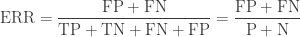
Accuracy
Accuracy (ACC) is calculated as the number of all correct predictions divided by the total number of the dataset. The best accuracy is 1.0, whereas the worst is 0.0. It can also be calculated by 1 – ERR.


Other basic measures from the confusion matrix
Error costs of positives and negatives are usually different. For instance, one wants to avoid false negatives more than false positives or vice versa. Other basic measures, such as sensitivity and specificity, are more informative than accuracy and error rate in such cases.
Sensitivity (Recall or True positive rate)
Sensitivity (SN) is calculated as the number of correct positive predictions divided by the total number of positives. It is also called recall (REC) or true positive rate (TPR). The best sensitivity is 1.0, whereas the worst is 0.0.


Specificity (True negative rate)
Specificity (SP) is calculated as the number of correct negative predictions divided by the total number of negatives. It is also called true negative rate (TNR). The best specificity is 1.0, whereas the worst is 0.0.


Precision (Positive predictive value)
Precision (PREC) is calculated as the number of correct positive predictions divided by the total number of positive predictions. It is also called positive predictive value (PPV). The best precision is 1.0, whereas the worst is 0.0.

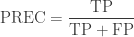
False positive rate
False positive rate (FPR) is calculated as the number of incorrect positive predictions divided by the total number of negatives. The best false positive rate is 0.0 whereas the worst is 1.0. It can also be calculated as 1 – specificity.

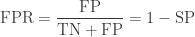
Correlation coefficient and F-score
Mathews correlation coefficient and F-score can be useful, but they are less frequently used than the other basic measures.
Matthews correlation coefficient
Matthews correlation coefficient (MCC) is a correlation coefficient calculated using all four values in the confusion matrix.
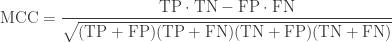
F-score
F-score is a harmonic mean of precision and recall.

β is commonly 0.5, 1, or 2.

An example of evaluation measure calculations
Let us assume that the outcome of some classification results in 6 TPs, 4 FNs, 8 TNs, and 2 FPs.

First, a confusion matrix is formed from the outcomes.
| Predicted | |||
| Positive | Negative | ||
| Observed | Positive | 6 | 4 |
| Negative | 2 | 8 |
Then, the calculations of basic measures are straightforward once the confusion matrix is created.
| measure | calculated value | |
|---|---|---|
| Error rate | ERR | 6 / 20 = 0.3 |
| Accuracy | ACC | 14 / 20 = 0.7 |
| Sensitivity True positive rate Recall |
SN TPR REC |
6 / 10 = 0.6 |
| Specificity True negative rate |
SP TNR |
8 / 10 = 0.8 |
| Precision Positive predictive value |
PREC PPV |
6 / 8 =0.75 |
| False positive rate | FPR | 2 / 10 = 0.2 |
Other evaluation measures
Please see the following pages for more advanced evaluation measures.
- Basic concept of model-wide evaluation
- Introduction to the ROC (Receiver Operating Characteristics) plot
- Introduction to the precision-recall plot
Delay-tolerant networks (DTNs) for satellite communications
C. Caini, in Advances in Delay-Tolerant Networks (DTNs) (Second Edition), 2021
2.3.4.4 PER and congestion
This environment suffers from congestion and PER simultaneously. Results are close to the congestion-only case, which shows that congestion is the dominant impairment.
Results of Fig. 2.3 prove the essential equivalence of DTN and PEP performance in the presence of continuous links, i.e., for fixed terminals, which is a fundamental result. It shows that DTN can provide the same goodput performance as the most effective and widely adopted solutions even in the absence of disruptions and/or network partitioning. The challenge here is the long RTT of the GEO satellite, which is enough to justify the adoption of DTN.
Read full chapter
URL:
https://www.sciencedirect.com/science/article/pii/B9780081027936000023
Transceiver Requirements
Shahin Farahani, in ZigBee Wireless Networks and Transceivers, 2008
4.2 Receiver Sensitivity
In the IEEE 802.15.4 standard, receiver sensitivity is defined as the lowest received signal power that yields a packet error rate (PER) of less than 1% [2]. IEEE 802.15.4 requires only −85 dBm of sensitivity for operations in the 2.4 GHz ISM band. In the 868/915 MHz band, if the BPSK modulation is used, the required sensitivity is −92 dBm. The optional modes of operation in the 868/915 MHz band (using ASK and OQPSK modulation) must meet −85 dBm of sensitivity.
If a 50 Ohm single-ended antenna is used, the sensitivity level of −85 dBm translates to a signal with effective (or rms) voltage of 12.6 uV:
Signal power=-85dBm=10(-85-3010)=3.16×10-12=3.16pW
Signal voltage=P×R=3.16×10-12×50=12.6uV
This means that any received signal with root-mean-square (rms) voltage of 12.6 uV or higher can be detected and the data can be extracted with a PER of less than 1%. During this test, no interference (Section 4.3) is present. Also, the PHY Service Data Unit (PSDU) length of the data packets used in this test must be 20 octets. Although it’s not required by the standard, the available commercial transceivers are capable of delivering −95 dBm to −100 dBm of sensitivity level.
Based on IEEE 802.15.4, receiver sensitivity is measured with a signal that has 0% error vector magnitude (EVM), whereas in reality, the signal may have an EVM of up to 35%, which is the maximum EVM allowed in IEEE 802.15.4. The EVM, discussed in Section 4.7, is an indication of the modulation inaccuracy. The EVM can worsen the sensitivity level, but as long as the EVM is below 35%, the sensitivity degradation should be less than 2 dB.
In IEEE 802.15.4, the carrier frequency offset of the input signal is zero during the receiver sensitivity test [2]. In reality, however, the input signal has some frequency offset and if the receiver does not use a frequency offset correction mechanism, the sensitivity level will be degraded. Figure 4.2 shows an example of receiver sensitivity degradation versus input carrier frequency offset when there is no offset correction.

Figure 4.2. Example of Receiver Sensitivity Degradation due to frequency offset
IEEE 802.15.4 not only defines the receiver minimum input signal lever (receiver sensitivity), it also determines the receiver maximum input level. A receiver must be able to receive signals with a power level of −20 dBm or higher and maintain PER of less than 1% to be compliant with IEEE 802.1.5.4.
Read full chapter
URL:
https://www.sciencedirect.com/science/article/pii/B9780750683937000042
Wireless Local Area Networks
Vijay K. Garg, in Wireless Communications & Networking, 2007
21.12.2 PER from M Neighboring IEEE 802.11 WLANs*
Under IEEE 802.11 FH, the probability of M IEEE 802.11 induced collisions on a Bluetooth packet is given as [17]:
(21.4)PER=1−{[1−|G|L]⋅(7879)⌈H/L⌉+|G|L⋅(5779)⌈H/L⌉−G/|G|}M
Under IEEE 802.11 DS, the probability of M IEEE 802.11 induced collisions on a Bluetooth packet is given as:
(21.5)PER=1−{[1−|G|L]⋅(5779)⌈H/L⌉+|G|L⋅(5779)⌈H/L⌉−G/|G|}M
where:
-
H = the duration of a Bluetooth packet
-
L = the dwell period of an IEEE 802.11 transmission
-
Tw = the packet duration of IEEE 802.11
-
G = ⌈H/L⌉L−Tw−H
-
⌈x⌉ = the least integer greater than or equal to x
The collision probability of a Bluetooth piconet where there are N neighboring Bluetooth piconets and M IEEE 802.11 WLANs will be:
(21.6)(PER)syn=1−[(7879)N⋅(Ps)M]
(21.7)(PER)asyn=1−(PsUR)N(Ps)M
Read full chapter
URL:
https://www.sciencedirect.com/science/article/pii/B9780123735805500557
Physical layer design
Husheng Li, in Communications for Control in Cyber Physical Systems, 2016
8.5.1 Motivation
Since the reliability of communication is usually very high in CPSs (e.g., in the wide area monitoring system in smart grids, the packet error rate should be less than 10−5 [166]) while the communication channel may experience various degradations (e.g., the harsh environments for communications in smart grids), it is important to use channel coding to protect the information transmission.
A straightforward approach for coding in a CPS is to follow the traditional procedure of separate quantization, coding, transmission, decoding, and further processing, which is adopted in conventional communication systems (Fig. 8.7). However, separate channel decoding and system state estimation may not be optimal when there exist redundancies in the transmitted messages. For example, the transmitted codeword at time t, b(t), is generated by the observation on the physical dynamics, y(t). Due to the time correlation of system states, y(t) is correlated with y(t + 1), thus being able to provide information for decoding the codeword in the next time slot t + 1. Hence if the decoding procedure is independent of the system state estimation, the permanence will be degraded due to the loss of redundancy. One may argue that the redundancy can be removed in the source coding procedure (e.g., encoding only the innovation vector in Kalman filtering if the physical dynamics is linear with Gaussian noise [167]). However, this requires substantial computation, which a sensor may not be able to carry out. Moreover, the sensor may not have the overall system parameters for the extraction of innovation information. Hence it is more desirable to shift the burden to the controller, which has more computational power and more system information; then the inexpensive sensor focuses on transmitting the raw data.

Fig. 8.7. Illustration of the components in a CPS.
In this section, we propose an algorithm for joint channel decoding and state estimation in a CPS. We consider traditional channel codes with memory (e.g., convolutional codes). Then the physical dynamics system state evolution and the channel codes can be considered as an equivalent concatenated code, as illustrated in Fig. 8.8, in which the outer code is the generation of system observation (we call it a “nature encoded” codeword) while the inner code is the traditional channel coding. The outer code is generated by the physical dynamics in an analog manner (since the value is continuous) while the inner code is carried out by a digital encoder. We will use belief propagation (BP) [168], which has been widely applied in decoding turbo codes and low-density parity-check (LDPC) codes, to decode this equivalent concatenated code. The major challenge is that the Bayesian inference is over a hybrid system which has both continuous- and discrete-valued nodes.

Fig. 8.8. Illustration of the equivalent concatenated code for system state evolution and channel coding.
Read full chapter
URL:
https://www.sciencedirect.com/science/article/pii/B9780128019504000081
Radio channel access challenges in LoRa low-power wide-area networks
Congduc Pham, … Muhammad Ehsan, in LPWAN Technologies for IoT and M2M Applications, 2020
4.2.1.1 Encoding
First, the binary source input bits pass through an encoder. The output of encoder depends on the choice of CR value. Encoding reduces the packet error rate in the presence of short bursts of interference. LoRa uses Hamming codes for FEC. These are linear block codes and are easy to implement. LoRa uses coding rates CR of 4/5, 2/3, 4/7, and 1/2, which means if the code rate is denoted as k/n, where k represents the number of useful information bits, and encoder generates n output bits, then (n−k) are the redundant bits. If we assume CR values between 1, 2, 3, and 4 for coding rates 4/5, 4/6, 4/7, and 4/8, respectively, then the error detection and correction capabilities are as shown in Table 4–1.
Table 4–1. Error detection and correction capabilities of LoRa.
| Coding rates | Error detection (bits) | Error correction (bits) |
|---|---|---|
| 4/5 | 0 | 0 |
| 4/6 | 1 | 0 |
| 4/7 | 2 | 1 |
| 4/8 | 3 | 1 |
Read full chapter
URL:
https://www.sciencedirect.com/science/article/pii/B9780128188804000041
LoRaWAN for smart cities: experimental study in a campus deployment
Rakshit Ramesh, … Bharadwaj Amrutur, in LPWAN Technologies for IoT and M2M Applications, 2020
15.3.1.4 Range and packet error rate for SF8–SF11
For the sake of brevity, we have only shown results of SF12 and SF7. Our experiments show that the range of network gradually increases with increase in SF and the PER for peripheral regions in each SF becomes smaller. In SF11 (comparing with Fig. 15–4), it is observed that region (G) is not covered by the network and region € experiences a PER of >80%. In SF8 (comparing with Fig. 15–3), it is observed that region (D) comes under the network coverage and PER of region C decreases to <80%. Likewise, the trends for SF9 and SF10 become increasingly better.
Read full chapter
URL:
https://www.sciencedirect.com/science/article/pii/B9780128188804000168
Long-term evolution for machines (LTE-M)
Suresh R. Borkar, in LPWAN Technologies for IoT and M2M Applications, 2020
7.3.6 Use of LTE priority structure for LTE-M applications
One of the distinctive features of LTE is the very versatile and robust priority assignment structure for user-traffic bearers. There are 13 priority levels ranging from 0.5 (highest) to 9 (lowest) supporting guaranteed bit–rate (GBR) and non-GBR (N-GBR) bearers [20]. The priority levels are characterized by varying combinations of packet delay and packet error rate (PER). Packet delays range from 50 to 300 milliseconds and a range of 10−2 to 10−6 is available for PER. The standards provide suggested mapping of various application classes to these priority levels but the network operators can apply their own discretion to assign the priority levels for their services. This is a strong and effective platform for managing the varying quality of service (QoS) requirements for LTE-M-based LPWAN services and provides a unique advantage to LTE-M.
Several classes of applications can be mapped for LTE-M usage. A representative mapping is suggested in Table 7–1. The best available PER of 10−6 is used since data integrity is very important for MTC type applications. This is paired with three options for packet delay—60, 100, and 300 milliseconds.
Table 7–1. Proposed LTE-M priority structure.
| 3GPP suggested service | Priority level | Est. packet delay (milliseconds) | Est. packet error rate | Suggested LTE-M application |
|---|---|---|---|---|
| Nonconversational video | 5 (GBR) | 300 | 10−6 | MTC 1 |
| IMS signaling | 1 (N-GBR) | 100 | 10−6 | MTC 2 |
| Mission-critical delay-sensitive signaling | 0.5 (N-GBR) | 60 | 10−6 | MTC 3 |
MTC1 are applications, which may be delay-tolerant, for example utility meters. MTC 3 type applications may be delay-sensitive, for example remote robotics surgery. MTC 2 can be applied to applications such as smart city which fall in between these two extreme attributes.
Read full chapter
URL:
https://www.sciencedirect.com/science/article/pii/B9780128188804000077
Quality of service control
Yali Guo, Tricci So, in 5G NR and Enhancements, 2022
13.5.2 Alternative quality of service profile
The QoS notification control mechanism can solve the problem of service interruption due to the bearer release when the QoS cannot be guaranteed. The 5G–AN sends the notification to the core network that the QoS cannot be guaranteed. But the interaction between the core network and the application is slow. Hence, it is uncertain whether or not the application will adjust the QoS requirements. The 5G–AN can only allocate resources to meet the original QoS requirements while waiting for the adjustment instructions from the core network. At this point, the allocation of resources by the 5G–AN could become unsustainable. Due to such consideration, the alternative QoS profile is introduced as part of the QoS notification control mechanism in the 5G system. Such QoS profile is used to make the 5G–AN aware of the alternative QoS profiles when the original QoS cannot be guaranteed, so as to further improve the efficiency of resource allocation.
An alternative QoS profile is an optional optimization that depends on the QoS notification control mechanism and is only used for GBR QoS Flows with QoS notification control enabled. The PCF provides one or more alternative QoS parameter sets in the PCC rules by interacting with the AF. Then the SMF generates one or more QoS profiles for the corresponding QoS Flow, and sends them to the 5G–AN.
When the QoS cannot be guaranteed, the 5G–AN evaluates whether the resources can be sustained by one of the alternative QoS profiles. If so, it will indicate the alternative QoS profile that can be guaranteed when sending notification to the SMF. The operation at the 5G–AN is as follows:
- 1.
-
When the GFBR, PDB, or PER of a QoS Flow cannot be guaranteed, the 5G–AN evaluates whether the radio resources can guarantee an alternative QoS profile one by one according to the priority of the alternative QoS profiles. If an alternative QoS profile can be guaranteed, the 5G–AN indicates to the SMF the first matched alternative QoS profile. If none of the alternative QoS profiles can be guaranteed, the 5G–AN indicates to the SMF that QoS requirements cannot be guaranteed and there is no viable alternative QoS profile.
- 2.
-
After that, when the 5G–AN determines that the currently fulfilled GFBR, PDB, or PER are different (better or worse) from the situation indicated in the last notification, the 5G–AN indicates the latest QoS status to the SMF again.
- 3.
-
The 5G–AN always tries to fulfill the QoS profile with any alternative QoS profile that has the highest priority to meet the current situation.
- 4.
-
The SMF needs to notify the PCF after receiving the notification from the 5G–AN.
- 5.
-
The SMF may also inform the UE about changes in the QoS parameters.
Read full chapter
URL:
https://www.sciencedirect.com/science/article/pii/B9780323910606000131
LoRaWAN protocol: specifications, security, and capabilities
Alper Yegin, … Nicolas Sornin, in LPWAN Technologies for IoT and M2M Applications, 2020
3.3.3 LoRaWAN network capacity and scaling
The Okumura–Hata model is the radio propagation model to simulate results as pictured in Fig. 3–6. It is valid for deployments for which the base station is installed at high outdoor locations compared to the height of surrounding buildings. Devices are assumed to have a 0 dBi antenna, which is typical for small devices. Our simulation uses 16 channels and targets a 10% packet error rate. Fig. 3–6 shows the random position of devices and color coding for their optimal spreading factor in a hexagonal network.

Figure 3–6. Simulated network layout with hexagonal tiling.
Fig. 3–7 shows the maximum capacity results for the network and a single cell. It confirms that capacity scales easily with the density of network gateways.

Figure 3–7. Impact of multicell deployment on capacity.
These results show that the future of LoRaWAN networks, particularly in urban environments where the noise floor is expected to rise due to increased traffic, is going toward microcellular networks, for example, with receivers integrated in triple-play modems. Macro-diversity provides not only higher capacity, see Fig. 3–8, but also greater resilience to interference and lower power consumption for end devices.

Figure 3–8. Evolution of capacity as intersite distance (ISD) becomes shorter (number of messages (in millions) vs ISD).
LoRaWAN provides a horizontal connectivity solution to address the wide-ranging needs of IoT applications for LPWAN deployments. However, these benefits are only possible with intelligent NS algorithms proprietary to network solution vendors.
Read full chapter
URL:
https://www.sciencedirect.com/science/article/pii/B978012818880400003X
Performance of IEEE 802.16m and 3GPP LTE-Advanced
Sassan Ahmadi, in Mobile WiMAX, 2011
12.9.7 IEEE 802.16m Link Budget
The IMT-Advanced submissions were required to provide a detailed link budget analysis under the ITU-R specified test environments. Report ITU-R M.2135-1 provided a methodology and common parameters in order to calculate the downlink and uplink link budgets. In addition to the common parameters, the following assumptions were made in the calculations:
- •
-
There are four transmit antennas and four receive antennas in the BS, and there are two transmit antennas and two 2 receive antennas in the MS.
- •
-
The target packet error rate is 10% for initial transmission of data channels, and 1% for the control channels.
- •
-
The modulation and coding scheme for the DL Assignment A-MAP is QPSK 1/8.
- •
-
There are 6 bits transmitted over the uplink primary fast-feedback channel.
- •
-
The MIMO scheme for downlink data is rank-1 wideband beamforming, for downlink control is SFBC with non-adaptive precoder, for uplink data is rank-1 wideband beamforming, and for uplink control is single antenna transmission.
- •
-
The permutation (subchannelization) scheme used for DL/UL data is mini-band CRU and for DL control is DRU.
- •
-
There is 2 dB pilot-boosting over data tones in the downlink, and no pilot boosting in the uplink.
- •
-
No HARQ is assumed for the control channel.
- •
-
0.5 dB HARQ combining gain for the data channel.
Shadowing fade margin is determined as a function of the cell edge coverage reliability and the standard deviation of the log-normal shadow-fading, including penetration loss. Cell edge coverage reliability is determined for the given area coverage reliability as a function of the shadow fading standard deviation and the path loss exponent obtained from the path loss model. The cell edge reliability can be determined using simulations or using traditional numerical methods. Cell area reliability is defined as the percentage of the cell area over which coverage can be guaranteed. It is obtained from the cell edge reliability, shadow fading standard deviation, and the path loss exponent. The latter two values are used to calculate a fade margin. Macro diversity gain may be considered explicitly in order to improve the system margin or implicitly by reducing the fade margin. The path loss models are summarized in Table A1-2 of Report ITU-R M.2135-1 [6]. The IEEE 802.16m link budget in the downlink and uplink under various deployment scenarios for the TDD mode is given in Table 12-17.
TABLE 12-17. IEEE 802.16m Link Budget in Various Test Environments for the TDD Duplex Scheme [2]
| InH | UMi | UMa | RMa | |||||
|---|---|---|---|---|---|---|---|---|
| Parameter | Downlink | Uplink | Downlink | Uplink | Downlink | Uplink | Downlink | Uplink |
| System Configuration | ||||||||
| Carrier Frequency (GHz) | 3.4 | 3.4 | 2.5 | 2.5 | 2 | 2 | 0.8 | 0.8 |
| BS Antenna Heights (m) | 6 | 6 | 10 | 10 | 25 | 25 | 35 | 35 |
| MS Antenna Heights (m) | 1.5 | 1.5 | 1.5 | 1.5 | 1.5 | 1.5 | 1.5 | 1.5 |
| Cell Area Reliability | 95% | 95% | 95% | 95% | 95% | 95% | 95% | 95% |
| Transmission Bit Rate for Control Channel (kbps) | 89.6 | 1.2 | 89.6 | 1.2 | 89.6 | 1.2 | 89.6 | 1.2 |
| Transmission Bit Rate for Data Channel (Mbps) | 20.23 | 0.98 | 7.53 | 0.21 | 7.53 | 0.21 | 7.53 | 0.21 |
| Target Packet Error Rate for Control Channels | 10−2 | 10−2 | 10−2 | 10−2 | 10−2 | 10−2 | 10−2 | 10−2 |
| Target Packet Error Rate for Data Channels | 10−1 | 10−1 | 10−1 | 10−1 | 10−1 | 10−1 | 10−1 | 10−1 |
| Spectral Efficiency (bits/s/Hz) for Data | 0.856 | 0.830 | 0.637 | 0.720 | 0.637 | 0.720 | 0.637 | 0.720 |
| Pathloss Model | NLoS | NLoS | NLoS | NLoS | NLoS | NLoS | NLoS | NLoS |
| Mobile Speed (km/h) | 3 | 3 | 3 | 3 | 30 | 30 | 120 | 120 |
| Feeder Loss (dB) | 2 | 2 | 2 | 2 | 2 | 2 | 2 | 2 |
| Transmitter | ||||||||
| Number of Transmit Antennas | 4 | 2 | 4 | 2 | 4 | 2 | 4 | 2 |
| Maximum Transmit Power per Antenna (dBm) | 18 | 18 | 38 | 21 | 43 | 21 | 43 | 21 |
| Total Transmit Power (dBm) | 24 | 21 | 44 | 24 | 49 | 24 | 49 | 24 |
| Transmitter Antenna Gain (dBi) | 0 | 0 | 17 | 0 | 17 | 0 | 17 | 0 |
| Transmitter Array Gain (dB) | 0 | 0 | 0 | 0 | 0 | 0 | 0 | 0 |
| Control Channel Power Boosting Gain (dB) | 0 | 0 | 0 | 0 | 0 | 0 | 0 | 0 |
| Data Channel Power Loss Due to Pilot/Control Boosting (dB) | 0.2734 | 0 | 0.2734 | 0 | 0.2734 | 0 | 0.2734 | 0 |
| Cable, Connector, Combiner, Body Losses, etc. (dB) | 3 | 1 | 3 | 1 | 3 | 1 | 3 | 1 |
| Control Channel EIRP (dBm) | 21 | 20 | 58 | 23 | 63 | 23 | 63 | 23 |
| Data Channel EIRP (dBm) | 20.73 | 20 | 57.73 | 23 | 62.73 | 23 | 62.73 | 23 |
| Receiver | ||||||||
| Number of Receive Antennas | 2 | 4 | 2 | 4 | 2 | 4 | 2 | 4 |
| Receiver Antenna Gain (dBi) | 0 | 0 | 0 | 17 | 0 | 17 | 0 | 17 |
| Cable, Connector, Combiner, Body Losses, etc. (dB) | 1 | 3 | 1 | 3 | 1 | 3 | 1 | 3 |
| Receiver Noise Figure (dB) | 7 | 5 | 7 | 5 | 7 | 5 | 7 | 5 |
| Thermal Noise Density (dBm/Hz) | −174 | −174 | −174 | −174 | −174 | −174 | −174 | −174 |
| Receiver Interference Density (dBm/Hz) | −174 | −174 | −165 | −166 | −165 | −166 | −165 | −166 |
| Total Noise Plus Interference Density (dBm/Hz) | −166.21 | −167.81 | −162.88 | −164.24 | −162.88 | −164.24 | −162.88 | −164.24 |
| Occupied Channel Bandwidth (MHz) | 37.81 | 3.15 | 18.90 | 0.79 | 18.90 | 0.79 | 18.90 | 0.79 |
| Effective Noise Power (dBm) | −90.43 | −102.82 | −90.11 | −105.27 | −90.11 | −105.27 | −90.11 | −105.27 |
| Required SNR for the Control Channel (dB) | −0.56 | −2.48 | −1.57 | −4.10 | −1.95 | −3.97 | −1.19 | −2.42 |
| Required SNR for the Data Channel (dB) | 1.41 | −0.24 | −1.05 | −0.96 | −0.21 | −0.82 | −0.70 | 0.37 |
| Receiver Implementation Margin (dB) | 2 | 2 | 2 | 2 | 2 | 2 | 2 | 2 |
| HARQ Gain for Control Channel (dB) | 0 | 0 | 0 | 0 | 0 | 0 | 0 | 0 |
| HARQ Gain for Data Channel (dB) | 0.5 | 0.5 | 0.5 | 0.5 | 0.5 | 0.5 | 0.5 | 0.5 |
| Receiver Sensitivity for Control Channel (dBm) | −89.00 | −103.30 | −89.68 | −107.37 | −90.06 | −107.24 | −89.30 | −105.69 |
| Receiver Sensitivity for Data Channel (dBm) | −87.52 | −101.57 | −89.66 | −104.73 | −88.82 | −104.59 | −89.31 | −103.40 |
| Hardware Link Budget for Control Channel (dB) | 110.00 | 123.30 | 147.68 | 147.37 | 153.06 | 147.24 | 152.30 | 145.69 |
| Hardware Link Budget for Data Channel (dB) | 108.25 | 121.57 | 147.39 | 144.73 | 151.55 | 144.59 | 152.04 | 143.40 |
| Calculation of Available Path Loss | ||||||||
| Lognormal Shadow Fading Standard Deviation (dB) | 4 | 4 | 4 | 4 | 7.8 | 7.8 | 9.4 | 9.4 |
| Shadow Fading Margin (dB) | 2.8 | 2.8 | 3.10 | 3.10 | 8.1 | 8.1 | 10.4 | 10.4 |
| BS Selection/Macro-Diversity Gain (dB) | 0 | 0 | 0 | 0 | 0 | 0 | 0 | 0 |
| Penetration Loss (dB) | 0 | 0 | 0 | 0 | 9 | 9 | 9 | 9 |
| Other Gains (dB) | 0 | 0 | 0 | 0 | 0 | 0 | 0 | 0 |
| Available Path Loss for Control Channel (dB) | 106.20 | 117.50 | 143.58 | 141.27 | 134.96 | 127.14 | 131.90 | 123.29 |
| Available Path Loss for Data Channel (dB) | 104.45 | 115.77 | 143.29 | 138.63 | 133.45 | 124.49 | 131.64 | 121.00 |
| Range/Coverage Efficiency Calculation | ||||||||
| Maximum Range for Control Channel (m) | 87.39 | 159.42 | 1030.29 | 891.56 | 891.93 | 562.90 | 2361.39 | 1412.39 |
| Maximum Range for Data Channel (m) | 79.65 | 145.37 | 1011.89 | 755.50 | 816.07 | 481.56 | 2323.96 | 1232.23 |
| Coverage Area for Control Channel (km2/site) | 0.02 | 0.08 | 3.33 | 2.50 | 2.50 | 0.99 | 17.52 | 6.27 |
| Coverage Area for Data Channel (km2/site) | 0.20 | 0.07 | 3.22 | 1.79 | 2.09 | 0.73 | 16.97 | 4.77 |
Read full chapter
URL:
https://www.sciencedirect.com/science/article/pii/B9780123749642100128