From Wikipedia, the free encyclopedia
Data reduction is the transformation of numerical or alphabetical digital information derived empirically or experimentally into a corrected, ordered, and simplified form. The purpose of data reduction can be two-fold: reduce the number of data records by eliminating invalid data or produce summary data and statistics at different aggregation levels for various applications.[1]
When information is derived from instrument readings there may also be a transformation from analog to digital form. When the data are already in digital form the ‘reduction’ of the data typically involves some editing, scaling, encoding, sorting, collating, and producing tabular summaries. When the observations are discrete but the underlying phenomenon is continuous then smoothing and interpolation are often needed. The data reduction is often undertaken in the presence of reading or measurement errors. Some idea of the nature of these errors is needed before the most likely value may be determined.
An example in astronomy is the data reduction in the Kepler satellite. This satellite records 95-megapixel images once every six seconds, generating dozens of megabytes of data per second, which is orders-of-magnitudes more than the downlink bandwidth of 550 kB/s. The on-board data reduction encompasses co-adding the raw frames for thirty minutes, reducing the bandwidth by a factor of 300. Furthermore, interesting targets are pre-selected and only the relevant pixels are processed, which is 6% of the total. This reduced data is then sent to Earth where it is processed further.
Research has also been carried out on the use of data reduction in wearable (wireless) devices for health monitoring and diagnosis applications. For example, in the context of epilepsy diagnosis, data reduction has been used to increase the battery lifetime of a wearable EEG device by selecting and only transmitting, EEG data that is relevant for diagnosis and discarding background activity.[2]
Types of Data Reduction[edit]
Dimensionality Reduction[edit]
When dimensionality increases, data becomes increasingly sparse while density and distance between points, critical to clustering and outlier analysis, becomes less meaningful. Dimensionality reduction helps reduce noise in the data and allows for easier visualization, such as the example below where 3-dimensional data is transformed into 2 dimensions to show hidden parts. One method of dimensionality reduction is wavelet transform, in which data is transformed to preserver relative distance between objects at different levels of resolution, and is often used for image compression.[3]

An example of dimensionality reduction.
Numerosity Reduction[edit]
This method of data reduction reduces the data volume by choosing alternate, smaller forms of data representation. Numerosity reduction can be split into 2 groups: parametric and non-parametric methods. Parametric methods (regression, for example) assume the data fits some model, estimate model parameters, store only the parameters, and discard the data. One example of this is in the image below, where the volume of data to be processed is reduced based on more specific criteria. Another example would be a log-linear model, obtaining a value at a point in m-D space as the product on appropriate marginal subspaces. Non-parametric methods do not assume models, some examples being histograms, clustering, sampling, etc.[4]

An example of data reduction via numerosity reduction
Statistical modelling[edit]
Data reduction can be obtained by assuming a statistical model for the data. Classical principles of data reduction include sufficiency, likelihood, conditionality and equivariance.[5]
See also[edit]
- Data cleansing
- Data editing
- Data pre-processing
- Data wrangling
References[edit]
- ^ «Travel Time Data Collection Handbook» (PDF). Retrieved 6 December 2020.
- ^ Iranmanesh, S.; Rodriguez-Villegas, E. (2017). «A 950 nW Analog-Based Data Reduction Chip for Wearable EEG Systems in Epilepsy». IEEE Journal of Solid-State Circuits. 52 (9): 2362–2373. doi:10.1109/JSSC.2017.2720636. hdl:10044/1/48764.
- ^ Han, J.; Kamber, M.; Pei, J. (2011). «Data Mining: Concepts and Techniques (3rd ed.)» (PDF). Retrieved 6 December 2020.
- ^ Han, J.; Kamber, M.; Pei, J. (2011). «Data Mining: Concepts and Techniques (3rd ed.)» (PDF). Retrieved 6 December 2020.
- ^ Casella, George (2002). Statistical inference. Roger L. Berger. Australia: Thomson Learning. pp. 271–309. ISBN 0-534-24312-6. OCLC 46538638.
Further reading[edit]
- Ehrenberg, Andrew S. C. (1982). A Primer in Data Reduction: An Introductory Statistics Textbook. New York: Wiley. ISBN 0-471-10134-6.
Data reduction is a process that reduced the volume of original data and represents it in a much smaller volume. Data reduction techniques ensure the integrity of data while reducing the data.
The time required for data reduction should not overshadow the time saved by the data mining on the reduced data set. In this section, we will discuss data reduction in brief and we will discuss different methods of data reduction.
Content: Data Reduction in Data Mining
- What is Data Reduction?
- Data Reduction Techniques
- Key Takeaways
What is Data Reduction?
When you collect data from different data warehouses for analysis, it results in a huge amount of data. It is difficult for a data analyst to deal with this large volume of data.
It is even difficult to run the complex queries on the huge amount of data as it takes a long time and sometimes it even becomes impossible to track the desired data.
This is why reducing data becomes important. Data reduction technique reduces the volume of data yet maintains the integrity of the data.
Data reduction does not affect the result obtained from data mining that means the result obtained from data mining before data reduction and after data reduction is the same (or almost the same).
The only difference occurs in the efficiency of data mining. Data reduction increases the efficiency of data mining. In the following section, we will discuss the techniques of data reduction.
Data Reduction Techniques
Techniques of data deduction include dimensionality reduction, numerosity reduction and data compression.
1. Dimensionality Reduction
Dimensionality reduction eliminates the attributes from the data set under consideration thereby reducing the volume of original data. In the section below, we will discuss three methods of dimensionality reduction.
a. Wavelet Transform
In the wavelet transform, a data vector X is transformed into a numerically different data vector X’ such that both X and X’ vectors are of the same length. Then how it is useful in reducing data?
The data obtained from the wavelet transform can be truncated. The compressed data is obtained by retaining the smallest fragment of the strongest of wavelet coefficients.
Wavelet transform can be applied to data cube, sparse data or skewed data.
b. Principal Component Analysis
Let us consider we have a data set to be analyzed that has tuples with n attributes, then the principal component analysis identifies k independent tuples with n attributes that can represent the data set.
In this way, the original data can be cast on a much smaller space. In this way, the dimensionality reduction can be achieved. Principal component analysis can be applied to sparse, and skewed data.
c. Attribute Subset Selection
The large data set has many attributes some of which are irrelevant to data mining or some are redundant. The attribute subset selection reduces the volume of data by eliminating the redundant and irrelevant attribute.
The attribute subset selection makes it sure that even after eliminating the unwanted attributes we get a good subset of original attributes such that the resulting probability of data distribution is as close as possible to the original data distribution using all the attributes.
2. Numerosity Reduction
The numerosity reduction reduces the volume of the original data and represents it in a much smaller form. This technique includes two types parametric and non-parametric numerosity reduction.
Parametric
Parametric numerosity reduction incorporates ‘storing only data parameters instead of the original data’. One method of parametric numerosity reduction is ‘regression and log-linear’ method.
- Regression and Log-Linear
Linear regression models a relationship between the two attributes by modelling a linear equation to the data set. Suppose we need to model a linear function between two attributes.
y = wx +b
Here, y is the response attribute and x is the predictor attribute. If we discuss in terms of data mining, the attribute x and the attribute y are the numeric database attributes whereas w and b are regression coefficients.
Multiple linear regression lets the response variable y to model linear function between two or more predictor variable.
Log-linear model discovers the relation between two or more discrete attributes in the database. Suppose, we have a set of tuples presented in n-dimensional space. Then the log-linear model is used to study the probability of each tuple in a multidimensional space.
Regression and log-linear method can be used for sparse data and skewed data.
Non-Parametric
- Histogram
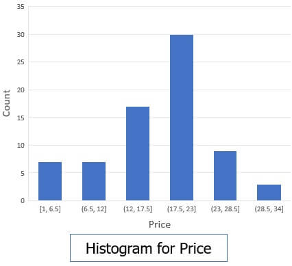
A histogram is a ‘graph’ that represents frequency distribution which describes how often a value appears in the data. Histogram uses the binning method and to represent data distribution of an attribute. It uses disjoint subset which we call as bin or buckets.
We have data for AllElectronics data set, which contains prices for regularly sold items.
1, 1, 5, 5, 5, 5, 5, 8, 8, 10, 10, 10, 10, 12, 14, 14, 14, 15, 15, 15, 15, 15, 15, 18, 18, 18, 18, 18, 18, 18, 18, 20, 20, 20, 20, 20, 20, 20, 21, 21, 21, 21, 25, 25, 25, 25, 25, 28, 28, 30, 30, 30.
The diagram below shows a histogram of equal width that shows the frequency of price distribution.
 A histogram is capable of representing dense, sparse, uniform or skewed data. Instead of only one attribute, the histogram can be implemented for multiple attributes. It can effectively represent the up to five attributes.
 A histogram is capable of representing dense, sparse, uniform or skewed data. Instead of only one attribute, the histogram can be implemented for multiple attributes. It can effectively represent the up to five attributes.
- Clustering
Clustering techniques groups the similar objects from the data in such a way that the objects in a cluster are similar to each other but they are dissimilar to objects in another cluster.
How much similar are the objects inside a cluster can be calculated by using a distance function. More is the similarity between the objects in a cluster closer they appear in the cluster.
The quality of cluster depends on the diameter of the cluster i.e. the at max distance between any two objects in the cluster.
The original data is replaced by the cluster representation. This technique is more effective if the present data can be classified into a distinct clustered.
- Sampling
One of the methods used for data reduction is sampling as it is capable to reduce the large data set into a much smaller data sample. Below we will discuss the different method in which we can sample a large data set D containing N tuples:
- Data Cube Aggregation
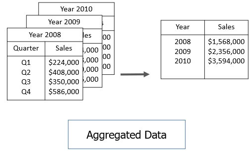
Consider you have the data of AllElectronics sales per quarter for the year 2008 to the year 2010. In case you want to get the annual sale per year then you just have to aggregate the sales per quarter for each year. In this way, aggregation provides you with the required data which is much smaller in size and thereby we achieve data reduction even without losing any data.
 The data cube aggregation is a multidimensional aggregation which eases multidimensional analysis. Like in the image below the data cube represent annual sale for each item for each branch. The data cube present precomputed and summarized data which eases the data mining into fast access.

 The data cube aggregation is a multidimensional aggregation which eases multidimensional analysis. Like in the image below the data cube represent annual sale for each item for each branch. The data cube present precomputed and summarized data which eases the data mining into fast access.
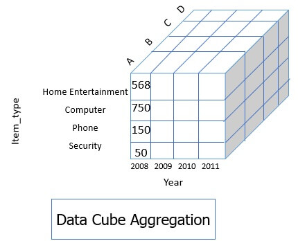
3. Data Compression
Data compression is a technique where the data transformation technique is applied to the original data in order to obtain compressed data. If the compressed data can again be reconstructed to form the original data without losing any information then it is a ‘lossless’ data reduction.
If you are unable to reconstruct the original data from the compressed one then your data reduction is ‘lossy’. Dimensionality and numerosity reduction method are also used for data compression.
Key Takeaways
- Data reduction is a method of reducing the volume of data thereby maintaining the integrity of the data.
- There are three basic methods of data reduction dimensionality reduction, numerosity reduction and data compression.
- The time taken for data reduction must not be overweighed by the time preserved by data mining on the reduced data set.
So, this is all about the data reduction and its techniques. We have covered different methods that can be employed for data reduction.
Top reviews from the United States
There was a problem filtering reviews right now. Please try again later.
Reviewed in the United States 🇺🇸 on June 10, 2008
Bevington’s book «Data Reduction and Error Analysis» is an old war-horse that is now in its third edition, and looks a good intermediate-level, practical reference to have on the shelf. I bought my copy only recently to follow up a reference, so am less familiar with it than I’d like to be before writing a review.
Unfortunately, following that reference led me to equation 4.22, which is wrong. When forming a weighted average of variances, one needs to square the weights in the numerator and square the sum of weights in the denominator. The equation as given has the first power of the weights and of the sum, just as found in the weighted mean. As I sort the matter out myself (with help from a friendly statistician) and look around at other treatments, this appears to be a common mistake, but mistake it is.
Otherwise, it seems a good book clearly written.
Reviewed in the United States 🇺🇸 on May 29, 2012
I had the good fortune to be trained by a physicist who, to my horror, left halfway through my bioinformatics PhD. (Imagine if Luke Skywalker were in the swamp, and Yoda told him he’d taken a job at the Broad.) Before he left, while I nearly collapsed in panic, he told me to get Bevington.
I have stacks of statistics books that teach readers to plug things into formulas. This is not the way to learn or do statistics, and in anything but the most trivial of cases will lead to incorrect results. Bevington teaches the reader to think about what the data looks like, and specifically the error and uncertainty in the data. This is far more valuable than knowing the formula for a chi-square test or whatever other rubbish is generally taught in statistics classes.
I would recommend this book as the first book that any scientist in training, in any field, read.
Reviewed in the United States 🇺🇸 on December 15, 2011
This is a book that has been widely used by three generations of students and researchers. I used the 1969 edition as an undergraduate. The 2003 paperback edition would be an equally excellent publication except for the astounding number of editing errors in formulas and a few gross errors that seem to be outright mistakes. One particularly egregious error concerning multiplication of linear matrices appears in appendix B. I bought the text as a refresher and reference. Because I had a working knowledge of the subject matter, most of the errors were immediately evident. However, someone new to the subject would find many of them confusing.
In My opinion, McGraw Hill has done a terrible disservice to the authors and should be embarrassed at doing such a poor job of publishing an otherwise excellent book.
Reviewed in the United States 🇺🇸 on January 5, 2015
This is the standard text for data analysis in physics at an advanced undergraduate or graduate level. Using the chi-square fits and F test sections of this book, I was able to fit transit models to light curves for known transiting exoplanets and reconstruct the radius ratio of the planet and the star, as well as obtain the statistical significance of that detection. This book is a good first place to look for all your physics statistics needs.
Reviewed in the United States 🇺🇸 on October 24, 2013
I still have the issue I came to use extensively back in the 70’s — and I still do. This new version keeps on being useful for both the undergrad and grad student and for the researcher: it presents everything in a plain but thorough way, and it is invaluable for a quick reference «mind reminder». I recommend it without any reservations — I bought one for my son!
Reviewed in the United States 🇺🇸 on April 1, 2018
My professor loved this book, but it’s very difficult and dense, and unfortunately, the examples in the text weren’t related to the experiments I was performing. I found it difficult to apply the readings to the experiments.
Reviewed in the United States 🇺🇸 on December 31, 2013
Book arrived in a timely manner and the used material was just as the summary described. I found it a good buy and satisfactory to my needs.
Reviewed in the United States 🇺🇸 on February 6, 2014
This is a must for experimental science. Also the online avaible codes are great. I wrote a good nonlinear least squares program that can fit almost any function to data. The resuls are ready for plotting in xmgrace.I strongly recommend this old classic.
-dgs
Top reviews from other countries
5.0 out of 5 stars
Nice book
Reviewed in Italy 🇮🇹 on October 10, 2022
The book is very nice. I think that an international exposition of error analisys is very important for physicists in this historical period. The seller had been very helpful and kind with me. I recommend this this book to all the students tha have to prepare laboratory exams.
3.0 out of 5 stars
Inhaltlich Spitzenklasse, wie auch schon die vorherige Version.
Reviewed in Germany 🇩🇪 on April 8, 2017
Inhaltlich ist das Buch Spitzenklasse (5 Sterne), wie auch schon die vorherige Version. (* * * * * )
(ohne Stern:)Nicht gefallen hat mir die Lieferung. Angepriesen als «Neu» und als Originalausgabe, kam ein indischer Billigdruck an. Dünnes Papier und kaum Druckerschwärze auf den Seiten — also eher «shades of grey» anstatt gut leserliche Buchstaben. Dazu die Vorder-und Rückseite des Buches mehrfach «operiert», d.h. Teile abgelöst (mit Skalpell oder Taschenmesser).
Da ich den Autor sehr schätze, das Buch dringend brauchte (sonst hätte ich retourniert) und das Buch inhaltlich wirklich super ist, habe ich es behalten…und später neu einbinden lassen.
5.0 out of 5 stars
Very nice book to learn the basics of error analysis and …
Reviewed in India 🇮🇳 on August 24, 2016
Very nice book to learn the basics of error analysis and data reduction. Recommend to all the science students Graduates and above
5.0 out of 5 stars
Data Reduction and Error Analysis for the Physical Sciences (Int’l Ed)
Reviewed in Germany 🇩🇪 on September 1, 2019
5.0 out of 5 stars
Great!
Reviewed in France 🇫🇷 on May 8, 2015
The books is easy to read. The concepts are well explained and illustrated with examples and exercises. If you need to know how to work properly with your experimental data, this book is for you.
Introduction
In today’s data-heavy systems, where everything is captured for future use, you get a mammoth data set on every load. This data set could be big in terms of observations or quite minuscule in terms of the number of features or columns, or both. Data mining becomes tedious in such cases, with only a few important features contributing to the value that you can take out of the data. Complex queries might take a long time to go through such huge data sets too. In such cases, a quick alternative is data reduction. Data reduction consciously allows us to categorize or extract the necessary information from a huge array of data to enable us to make conscious decisions.
In this article, we’ll explore
- What is Data Reduction?
- Data Reduction Techniques
1. What Is Data Reduction?
According to Wikipedia, a formal definition of Data Reduction goes like this, “Data reduction is the transformation of numerical or alphabetical digital information derived empirically or experimentally into a corrected, ordered, and simplified form.” In simple terms, it simply means large amounts of data are cleaned, organized and categorized based on prerequisite criteria to help in driving business decisions.
2. Data Reduction Techniques
 1")
There are two primary methods of Data Reduction, Dimensionality Reduction and Numerosity Reduction.
 2")
A) Dimensionality Reduction
Dimensionality Reduction is the process of reducing the number of dimensions the data is spread across. It means, the attributes or features, that the data set carries as the number of dimensions increases the sparsity. This sparsity is critical to clustering, outlier analysis and other algorithms. With reduced dimensionality, it is easy to visualize and manipulate data. There are three types of Dimensionality reduction.
- Wavelet Transform
Wavelet Transform is a lossy method for dimensionality reduction, where a data vector X is transformed into another vector X’, in such a way that both X and X’ still represent the same length. The result of wavelet transform can be truncated, unlike its original, thus achieving dimensionality reduction. Wavelet transforms are well suited for data cube, sparse data or data which is highly skewed. Wavelet transform is often used in image compression.
- Principal Component Analysis
This method involves the identification of a few independent tuples with ‘n’ attributes that can represent the entire data set. This method can be applied to skewed and sparse data.
- Attribute Subset Selection
Here, attributes irrelevant to data mining or redundant ones are not included in a core attribute subset. The core attribute subset selection reduces the data volume and dimensionality.
B) Numerosity Reduction
This method uses alternate, small forms of data representation, thus reducing data volume. There are two types of Numerosity reduction, Parametric and Non-Parametric.
- Parametric
This method assumes a model into which the data fits. Data model parameters are estimated, and only those parameters are stored, and the rest of the data is discarded. For example, a regression model can be used to achieve Parametric reduction if the data fits the Linear Regression model.
Linear Regression models a linear relationship between two attributes of the data set. Let’s say we need to fit a linear regression model between two attributes, x and y, where y is the dependent attribute, and x is the independent attribute or predictor attribute. The model can be represented by the equation y=wx b. Where w and b are regression coefficients. A multiple linear regression model lets us express the attribute y in terms of multiple predictor attributes.
Another method, the Log-Linear model discovers the relationship between two or more discrete attributes. Assume, we have a set of tuples in n-dimensional space; the log-linear model helps to derive the probability of each tuple in this n-dimensional space.
- Non-Parametric
A non-parametric numerosity reduction technique does not assume any model. The non-Parametric technique results in a more uniform reduction, irrespective of data size, but it may not achieve a high volume of data reduction like the Parametric one. There are at least four types of Non-Parametric data reduction techniques, Histogram, Clustering, Sampling, Data Cube Aggregation, Data Compression.
C) Histogram
 3")
A histogram can be used to represent dense, sparse, skewed or uniform data, involving multiple attributes, effectively up to 5 together.
D) Clustering
In Clustering, the data set is replaced by the cluster representation, where the data is split between clusters depending on similarities to each other within-cluster and dissimilarities to other clusters. The more the similarity within-cluster, the closer they appear within the cluster. The quality of the cluster depends on the maximum distance between any two data items in the cluster.
 4")
 5")
E) Sampling
Sampling is capable of reducing large data set into smaller sample data sets, reducing it to a representation of the original data set. There are four types of sampling data reduction methods.
- Simple Random Sample Without Replacement of sizes
- Simple Random Sample with Replacement of sizes
- Cluster Sample
- Stratified Sample
F) Data Cube Aggregation
Data Cube Aggregation is a multidimensional aggregation that uses aggregation at various levels of a data cube to represent the original data set, thus achieving data reduction. Data Cube Aggregation, where the data cube is a much more efficient way of storing data, thus achieving data reduction, besides faster aggregation operations.
G) Data Compression
It employs modification, encoding or converting the structure of data in a way that consumes less space. Data compression involves building a compact representation of information by removing redundancy and representing data in binary form. Data that can be restored successfully from its compressed form is called Lossless compression while the opposite where it is not possible to restore the original form from the compressed form is Lossy compression.
Conclusion
Data reduction achieves a reduction in volume, making it easy to represent and run data through advanced analytical algorithms. Data reduction also helps in the deduplication of data reducing the load on storage and the algorithms serving data science techniques downstream. It can be achieved in two principal ways. One by reducing the number of data records, or the features and the other by generating summary data and statistics at different levels.
If you are interested in making a career in the Data Science domain, our 11-month in-person Postgraduate Certificate Diploma in Data Science course can help you immensely in becoming a successful Data Science professional.
Also Read
- What is Data Processing? An Important Overview In 6 Points