Evaluation metrics
Here is a typical speaker diarization pipeline:
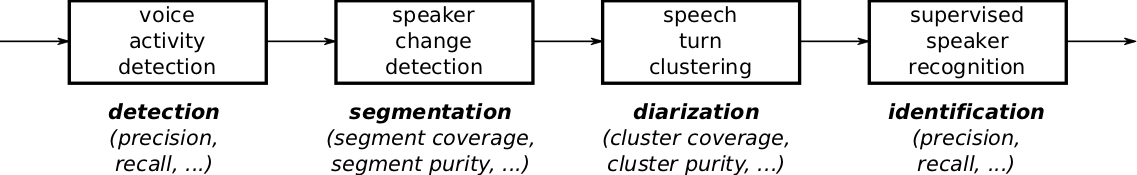
The first step is usually dedicated to speech activity detection, where the objective is to get rid of all non-speech regions.
Then, speaker change detection aims at segmenting speech regions into homogeneous segments.
The subsequent clustering step tries to group those speech segments according to the identity of the speaker.
Finally, an optional supervised classification step may be applied to actually identity every speaker cluster in a supervised way.
Looking at the final performance of the system is usually not enough for diagnostic purposes.
In particular, it is often necessary to evaluate the performance of each module separately to identify their strenght and weakness, or to estimate the influence of their errors on the complete pipeline.
Here, we provide the list of metrics that were implemented in pyannote.metrics with that very goal in mind.
Because manual annotations cannot be precise at the audio sample level, it is common in speaker diarization research to remove from evaluation a 500ms collar around each speaker turn boundary (250ms before and after).
Most of the metrics available in pyannote.metrics support a collar parameter, which defaults to 0.
Moreover, though audio files can always be processed entirely (from beginning to end), there are cases where reference annotations are only available for some regions of the audio files.
All metrics support the provision of an evaluation map that indicate which part of the audio file should be evaluated.
Detection
The two primary metrics for evaluating speech activity detection modules are detection error rate and detection cost function.
Detection error rate (not to be confused with diarization error rate) is defined as:
[text{detection error rate} = frac{text{false alarm} + text{missed detection}}{text{total}}]
where (text{false alarm}) is the duration of non-speech incorrectly classified as speech, (text{missed detection}) is the duration of speech incorrectly classified as non-speech, and (text{total}) is the total duration of speech in the reference.
Alternately, speech activity module output may be evaluated in terms of detection cost function, which is defined as:
[text{detection cost function} = 0.25 times text{false alarm rate} + 0.75 times text{miss rate}]
where (text{false alarm rate}) is the proportion of non-speech incorrectly classified as speech and (text{miss rate}) is the proportion of speech incorrectly classified as non-speech.
Additionally, detection may be evaluated in terms of accuracy (proportion of the input signal correctly classified), precision (proportion of detected speech that is speech), and recall (proporton of speech that is detected).
-
class
pyannote.metrics.detection.DetectionAccuracy(collar=0.0, skip_overlap=False, **kwargs)[source]¶ -
Detection accuracy
This metric can be used to evaluate binary classification tasks such as
speech activity detection, for instance. Inputs are expected to only
contain segments corresponding to the positive class (e.g. speech regions).
Gaps in the inputs considered as the negative class (e.g. non-speech
regions).It is computed as (tp + tn) / total, where tp is the duration of true
positive (e.g. speech classified as speech), tn is the duration of true
negative (e.g. non-speech classified as non-speech), and total is the total
duration of the input signal.- Parameters:
-
-
collar (float, optional) – Duration (in seconds) of collars removed from evaluation around
boundaries of reference segments (one half before, one half after). -
skip_overlap (bool, optional) – Set to True to not evaluate overlap regions.
Defaults to False (i.e. keep overlap regions).
-
-
compute_components(reference, hypothesis, uem=None, **kwargs)[source]¶ -
Compute metric components
- Parameters:
-
-
reference (type depends on the metric) – Manual reference
-
hypothesis (same as reference) – Evaluated hypothesis
-
- Returns:
-
components – Dictionary where keys are component names and values are component
values - Return type:
-
dict
-
compute_metric(detail)[source]¶ -
Compute metric value from computed components
- Parameters:
-
components (dict) – Dictionary where keys are components names and values are component
values - Returns:
-
value – Metric value
- Return type:
-
type depends on the metric
-
class
pyannote.metrics.detection.DetectionCostFunction(collar=0.0, skip_overlap=False, fa_weight=0.25, miss_weight=0.75, **kwargs)[source]¶ -
Detection cost function.
This metric can be used to evaluate binary classification tasks such as
speech activity detection. Inputs are expected to only contain segments
corresponding to the positive class (e.g. speech regions). Gaps in the
inputs considered as the negative class (e.g. non-speech regions).Detection cost function (DCF), as defined by NIST for OpenSAT 2019, is
0.25*far + 0.75*missr, where far is the false alarm rate
(i.e., the proportion of non-speech incorrectly classified as speech)
and missr is the miss rate (i.e., the proportion of speech incorrectly
classified as non-speech.- Parameters:
-
-
collar (float, optional) – Duration (in seconds) of collars removed from evaluation around
boundaries of reference segments (one half before, one half after).
Defaults to 0.0. -
skip_overlap (bool, optional) – Set to True to not evaluate overlap regions.
Defaults to False (i.e. keep overlap regions). -
fa_weight (float, optional) – Weight for false alarm rate.
Defaults to 0.25. -
miss_weight (float, optional) – Weight for miss rate.
Defaults to 0.75. -
kwargs – Keyword arguments passed to
pyannote.metrics.base.BaseMetric.
-
References
“OpenSAT19 Evaluation Plan v2.” https://www.nist.gov/system/files/documents/2018/11/05/opensat19_evaluation_plan_v2_11-5-18.pdf
-
compute_components(reference, hypothesis, uem=None, **kwargs)[source]¶ -
Compute metric components
- Parameters:
-
-
reference (type depends on the metric) – Manual reference
-
hypothesis (same as reference) – Evaluated hypothesis
-
- Returns:
-
components – Dictionary where keys are component names and values are component
values - Return type:
-
dict
-
compute_metric(components)[source]¶ -
Compute metric value from computed components
- Parameters:
-
components (dict) – Dictionary where keys are components names and values are component
values - Returns:
-
value – Metric value
- Return type:
-
type depends on the metric
-
class
pyannote.metrics.detection.DetectionErrorRate(collar=0.0, skip_overlap=False, **kwargs)[source]¶ -
Detection error rate
This metric can be used to evaluate binary classification tasks such as
speech activity detection, for instance. Inputs are expected to only
contain segments corresponding to the positive class (e.g. speech regions).
Gaps in the inputs considered as the negative class (e.g. non-speech
regions).It is computed as (fa + miss) / total, where fa is the duration of false
alarm (e.g. non-speech classified as speech), miss is the duration of
missed detection (e.g. speech classified as non-speech), and total is the
total duration of the positive class in the reference.- Parameters:
-
-
collar (float, optional) – Duration (in seconds) of collars removed from evaluation around
boundaries of reference segments (one half before, one half after). -
skip_overlap (bool, optional) – Set to True to not evaluate overlap regions.
Defaults to False (i.e. keep overlap regions).
-
-
compute_components(reference, hypothesis, uem=None, **kwargs)[source]¶ -
Compute metric components
- Parameters:
-
-
reference (type depends on the metric) – Manual reference
-
hypothesis (same as reference) – Evaluated hypothesis
-
- Returns:
-
components – Dictionary where keys are component names and values are component
values - Return type:
-
dict
-
compute_metric(detail)[source]¶ -
Compute metric value from computed components
- Parameters:
-
components (dict) – Dictionary where keys are components names and values are component
values - Returns:
-
value – Metric value
- Return type:
-
type depends on the metric
-
class
pyannote.metrics.detection.DetectionPrecision(collar=0.0, skip_overlap=False, **kwargs)[source]¶ -
Detection precision
This metric can be used to evaluate binary classification tasks such as
speech activity detection, for instance. Inputs are expected to only
contain segments corresponding to the positive class (e.g. speech regions).
Gaps in the inputs considered as the negative class (e.g. non-speech
regions).It is computed as tp / (tp + fp), where tp is the duration of true positive
(e.g. speech classified as speech), and fp is the duration of false
positive (e.g. non-speech classified as speech).- Parameters:
-
-
collar (float, optional) – Duration (in seconds) of collars removed from evaluation around
boundaries of reference segments (one half before, one half after). -
skip_overlap (bool, optional) – Set to True to not evaluate overlap regions.
Defaults to False (i.e. keep overlap regions).
-
-
compute_components(reference, hypothesis, uem=None, **kwargs)[source]¶ -
Compute metric components
- Parameters:
-
-
reference (type depends on the metric) – Manual reference
-
hypothesis (same as reference) – Evaluated hypothesis
-
- Returns:
-
components – Dictionary where keys are component names and values are component
values - Return type:
-
dict
-
compute_metric(detail)[source]¶ -
Compute metric value from computed components
- Parameters:
-
components (dict) – Dictionary where keys are components names and values are component
values - Returns:
-
value – Metric value
- Return type:
-
type depends on the metric
-
class
pyannote.metrics.detection.DetectionPrecisionRecallFMeasure(collar=0.0, skip_overlap=False, beta=1.0, **kwargs)[source]¶ -
Compute detection precision and recall, and return their F-score
- Parameters:
-
-
collar (float, optional) – Duration (in seconds) of collars removed from evaluation around
boundaries of reference segments (one half before, one half after). -
skip_overlap (bool, optional) – Set to True to not evaluate overlap regions.
Defaults to False (i.e. keep overlap regions). -
beta (float, optional) – When beta > 1, greater importance is given to recall.
When beta < 1, greater importance is given to precision.
Defaults to 1.
-
See also
pyannote.metrics.detection.DetectionPrecision,pyannote.metrics.detection.DetectionRecall,pyannote.metrics.base.f_measure-
compute_components(reference, hypothesis, uem=None, **kwargs)[source]¶ -
Compute metric components
- Parameters:
-
-
reference (type depends on the metric) – Manual reference
-
hypothesis (same as reference) – Evaluated hypothesis
-
- Returns:
-
components – Dictionary where keys are component names and values are component
values - Return type:
-
dict
-
compute_metric(detail)[source]¶ -
Compute metric value from computed components
- Parameters:
-
components (dict) – Dictionary where keys are components names and values are component
values - Returns:
-
value – Metric value
- Return type:
-
type depends on the metric
-
class
pyannote.metrics.detection.DetectionRecall(collar=0.0, skip_overlap=False, **kwargs)[source]¶ -
Detection recall
This metric can be used to evaluate binary classification tasks such as
speech activity detection, for instance. Inputs are expected to only
contain segments corresponding to the positive class (e.g. speech regions).
Gaps in the inputs considered as the negative class (e.g. non-speech
regions).It is computed as tp / (tp + fn), where tp is the duration of true positive
(e.g. speech classified as speech), and fn is the duration of false
negative (e.g. speech classified as non-speech).- Parameters:
-
-
collar (float, optional) – Duration (in seconds) of collars removed from evaluation around
boundaries of reference segments (one half before, one half after). -
skip_overlap (bool, optional) – Set to True to not evaluate overlap regions.
Defaults to False (i.e. keep overlap regions).
-
-
compute_components(reference, hypothesis, uem=None, **kwargs)[source]¶ -
Compute metric components
- Parameters:
-
-
reference (type depends on the metric) – Manual reference
-
hypothesis (same as reference) – Evaluated hypothesis
-
- Returns:
-
components – Dictionary where keys are component names and values are component
values - Return type:
-
dict
-
compute_metric(detail)[source]¶ -
Compute metric value from computed components
- Parameters:
-
components (dict) – Dictionary where keys are components names and values are component
values - Returns:
-
value – Metric value
- Return type:
-
type depends on the metric
Segmentation
Change detection modules can be evaluated using two pairs of dual metrics: precision and recall, or purity and coverage.
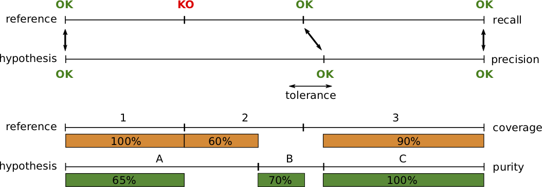
Precision and recall are standard metrics based on the number of correctly detected speaker boundaries. Recall is 75% because 3 out of 4 reference boundaries were correctly detected, and precision is 100% because all hypothesized boundaries are correct.
The main weakness of that pair of metrics (and their combination into a f-score) is that it is very sensitive to the tolerance parameter, i.e. the maximum distance between two boundaries for them to be matched. From one segmentation paper to another, authors may used very different values, thus making the approaches difficult to compare.
Instead, we think that segment-wise purity and coverage should be used instead.
They have several advantages over precision and recall, including the fact that they do not depend on any tolerance parameter, and that they directly relate to the cluster-wise purity and coverage used for evaluating speaker diarization.
Segment-wise coverage is computed for each segment in the reference as the ratio of the duration of the intersection with the most co-occurring hypothesis segment and the duration of the reference segment.
For instance, coverage for reference segment 1 is 100% because it is entirely covered by hypothesis segment A.
Purity is the dual metric that indicates how pure hypothesis segments are. For instance, segment A is only 65% pure because it is covered at 65% by segment 1 and 35% by segment 2.
The final values are duration-weighted average over each segment.
-
class
pyannote.metrics.segmentation.SegmentationCoverage(tolerance=0.5, **kwargs)[source]¶ -
Segmentation coverage
- Parameters:
-
tolerance (float, optional) – When provided, preprocess reference by filling intra-label gaps shorter
than tolerance (in seconds).
-
compute_components(reference, hypothesis, **kwargs)[source]¶ -
Compute metric components
- Parameters:
-
-
reference (type depends on the metric) – Manual reference
-
hypothesis (same as reference) – Evaluated hypothesis
-
- Returns:
-
components – Dictionary where keys are component names and values are component
values - Return type:
-
dict
-
compute_metric(detail)[source]¶ -
Compute metric value from computed components
- Parameters:
-
components (dict) – Dictionary where keys are components names and values are component
values - Returns:
-
value – Metric value
- Return type:
-
type depends on the metric
-
class
pyannote.metrics.segmentation.SegmentationPrecision(tolerance=0.0, **kwargs)[source]¶ -
Segmentation precision
>>> from pyannote.core import Timeline, Segment
>>> from pyannote.metrics.segmentation import SegmentationPrecision
>>> precision = SegmentationPrecision()
>>> reference = Timeline()
>>> reference.add(Segment(0, 1))
>>> reference.add(Segment(1, 2))
>>> reference.add(Segment(2, 4))
>>> hypothesis = Timeline()
>>> hypothesis.add(Segment(0, 1))
>>> hypothesis.add(Segment(1, 2))
>>> hypothesis.add(Segment(2, 3))
>>> hypothesis.add(Segment(3, 4))
>>> precision(reference, hypothesis)
0.6666666666666666
>>> hypothesis = Timeline()
>>> hypothesis.add(Segment(0, 4))
>>> precision(reference, hypothesis)
1.0
-
compute_components(reference, hypothesis, **kwargs)[source]¶ -
Compute metric components
- Parameters:
-
-
reference (type depends on the metric) – Manual reference
-
hypothesis (same as reference) – Evaluated hypothesis
-
- Returns:
-
components – Dictionary where keys are component names and values are component
values - Return type:
-
dict
-
compute_metric(detail)[source]¶ -
Compute metric value from computed components
- Parameters:
-
components (dict) – Dictionary where keys are components names and values are component
values - Returns:
-
value – Metric value
- Return type:
-
type depends on the metric
-
-
class
pyannote.metrics.segmentation.SegmentationPurity(tolerance=0.5, **kwargs)[source]¶ -
Segmentation purity
- Parameters:
-
tolerance (float, optional) – When provided, preprocess reference by filling intra-label gaps shorter
than tolerance (in seconds).
-
compute_components(reference, hypothesis, **kwargs)[source]¶ -
Compute metric components
- Parameters:
-
-
reference (type depends on the metric) – Manual reference
-
hypothesis (same as reference) – Evaluated hypothesis
-
- Returns:
-
components – Dictionary where keys are component names and values are component
values - Return type:
-
dict
-
class
pyannote.metrics.segmentation.SegmentationPurityCoverageFMeasure(tolerance=0.5, beta=1, **kwargs)[source]¶ -
Compute segmentation purity and coverage, and return their F-score.
- Parameters:
-
-
tolerance (float, optional) – When provided, preprocess reference by filling intra-label gaps shorter
than tolerance (in seconds). -
beta (float, optional) – When beta > 1, greater importance is given to coverage.
When beta < 1, greater importance is given to purity.
Defaults to 1.
-
See also
pyannote.metrics.segmentation.SegmentationPurity,pyannote.metrics.segmentation.SegmentationCoverage,pyannote.metrics.base.f_measure-
compute_components(reference, hypothesis, **kwargs)[source]¶ -
Compute metric components
- Parameters:
-
-
reference (type depends on the metric) – Manual reference
-
hypothesis (same as reference) – Evaluated hypothesis
-
- Returns:
-
components – Dictionary where keys are component names and values are component
values - Return type:
-
dict
-
compute_metric(detail)[source]¶ -
Compute metric value from computed components
- Parameters:
-
components (dict) – Dictionary where keys are components names and values are component
values - Returns:
-
value – Metric value
- Return type:
-
type depends on the metric
-
class
pyannote.metrics.segmentation.SegmentationRecall(tolerance=0.0, **kwargs)[source]¶ -
Segmentation recall
>>> from pyannote.core import Timeline, Segment
>>> from pyannote.metrics.segmentation import SegmentationRecall
>>> recall = SegmentationRecall()
>>> reference = Timeline()
>>> reference.add(Segment(0, 1))
>>> reference.add(Segment(1, 2))
>>> reference.add(Segment(2, 4))
>>> hypothesis = Timeline()
>>> hypothesis.add(Segment(0, 1))
>>> hypothesis.add(Segment(1, 2))
>>> hypothesis.add(Segment(2, 3))
>>> hypothesis.add(Segment(3, 4))
>>> recall(reference, hypothesis)
1.0
>>> hypothesis = Timeline()
>>> hypothesis.add(Segment(0, 4))
>>> recall(reference, hypothesis)
0.0
-
compute_components(reference, hypothesis, **kwargs)[source]¶ -
Compute metric components
- Parameters:
-
-
reference (type depends on the metric) – Manual reference
-
hypothesis (same as reference) – Evaluated hypothesis
-
- Returns:
-
components – Dictionary where keys are component names and values are component
values - Return type:
-
dict
-
Diarization
Diarization error rate (DER) is the emph{de facto} standard metric for evaluating and comparing speaker diarization systems.
It is defined as follows:
[text{DER} = frac{text{false alarm} + text{missed detection} + text{confusion}}{text{total}}]
where (text{false alarm}) is the duration of non-speech incorrectly classified as speech, (text{missed detection}) is the duration of
speech incorrectly classified as non-speech, (text{confusion}) is the duration of speaker confusion, and (text{total}) is the sum over all speakers of their reference speech duration.
Note that this metric does take overlapping speech into account, potentially leading to increased missed detection in case the speaker diarization system does not include an overlapping speech detection module.
Optimal vs. greedy
Two implementations of the diarization error rate are available (optimal and greedy), depending on how the one-to-one mapping between reference and hypothesized speakers is computed.
The optimal version uses the Hungarian algorithm to compute the mapping that minimize the confusion term, while the greedy version operates in a greedy manner, mapping reference and hypothesized speakers iteratively, by decreasing value of their cooccurrence duration.
In practice, the greedy version is much faster than the optimal one, especially for files with a large number of speakers – though it may slightly over-estimate the value of the diarization error rate.
Purity and coverage
While the diarization error rate provides a convenient way to compare different diarization approaches, it is usually not enough to understand the type of errors commited by the system.
Purity and coverage are two dual evaluation metrics that provide additional insight on the behavior of the system.
[begin{split} text{purity} & = & frac{displaystyle sum_{text{cluster}} max_{text{speaker}} |text{cluster} cap text{speaker}| }{displaystyle sum_{text{cluster}} |text{cluster}|} \
text{coverage} & = & frac{displaystyle sum_{text{speaker}} max_{text{cluster}} |text{speaker} cap text{cluster}| }{displaystyle sum_{text{speaker}} |text{speaker}|} \end{split}]
where (|text{speaker}|) (respectively (|text{cluster}|)) is the speech duration of this particular reference speaker (resp. hypothesized cluster), and (|text{speaker} cap text{cluster}|) is the duration of their intersection.
Over-segmented results (e.g. too many speaker clusters) tend to lead to high purity and low coverage, while under-segmented results (e.g. when two speakers are merged into one large cluster) lead to low purity and higher coverage.
Use case
This figure depicts the evolution of a multi-stage speaker diarization system applied on the ETAPE dataset.
It is roughly made of four consecutive modules (segmentation, BIC clustering, Viterbi resegmentation, and CLR clustering).
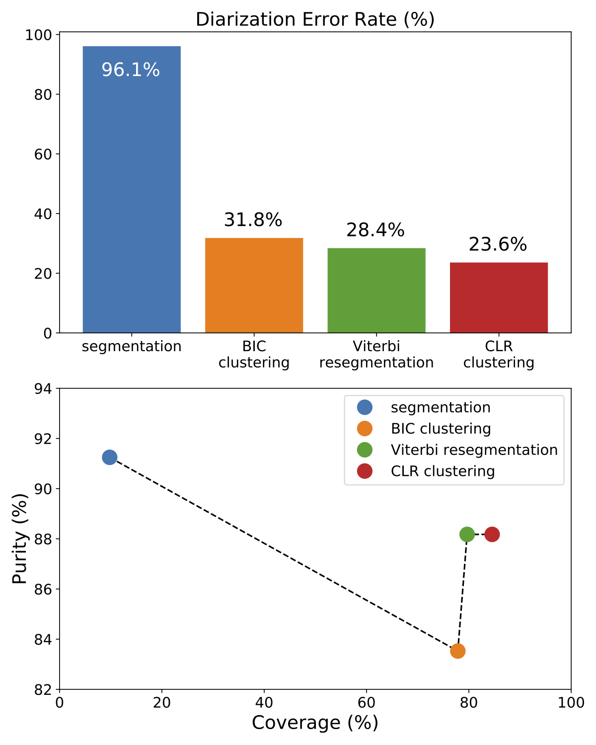
From the upper part of the figure (DER as a function of the module), it is clear that each module improves the output of the previous one.
Yet, the lower part of the figure clarifies the role of each module.
BIC clustering tends to increase the size of the speaker clusters, at the expense of purity (-7%).
Viterbi resegmentation addresses this limitation and greatly improves cluster purity (+5%), with very little impact on the actual cluster coverage (+2%).
Finally, CLR clustering brings an additional +5% coverage improvement.
Metrics for diarization
-
class
pyannote.metrics.diarization.DiarizationCompleteness(collar=0.0, skip_overlap=False, **kwargs)[source]¶ -
Cluster completeness
- Parameters:
-
-
collar (float, optional) – Duration (in seconds) of collars removed from evaluation around
boundaries of reference segments. -
skip_overlap (bool, optional) – Set to True to not evaluate overlap regions.
Defaults to False (i.e. keep overlap regions).
-
-
compute_components(reference, hypothesis, uem=None, **kwargs)[source]¶ -
Compute metric components
- Parameters:
-
-
reference (type depends on the metric) – Manual reference
-
hypothesis (same as reference) – Evaluated hypothesis
-
- Returns:
-
components – Dictionary where keys are component names and values are component
values - Return type:
-
dict
-
class
pyannote.metrics.diarization.DiarizationCoverage(collar=0.0, skip_overlap=False, weighted=True, **kwargs)[source]¶ -
Cluster coverage
A hypothesized annotation has perfect coverage if all segments from a
given reference label are clustered in the same cluster.- Parameters:
-
-
weighted (bool, optional) – When True (default), each cluster is weighted by its overall duration.
-
collar (float, optional) – Duration (in seconds) of collars removed from evaluation around
boundaries of reference segments. -
skip_overlap (bool, optional) – Set to True to not evaluate overlap regions.
Defaults to False (i.e. keep overlap regions).
-
-
compute_components(reference, hypothesis, uem=None, **kwargs)[source]¶ -
Compute metric components
- Parameters:
-
-
reference (type depends on the metric) – Manual reference
-
hypothesis (same as reference) – Evaluated hypothesis
-
- Returns:
-
components – Dictionary where keys are component names and values are component
values - Return type:
-
dict
-
class
pyannote.metrics.diarization.DiarizationErrorRate(collar=0.0, skip_overlap=False, **kwargs)[source]¶ -
Diarization error rate
First, the optimal mapping between reference and hypothesis labels
is obtained using the Hungarian algorithm. Then, the actual diarization
error rate is computed as the identification error rate with each hypothesis
label translated into the corresponding reference label.- Parameters:
-
-
collar (float, optional) – Duration (in seconds) of collars removed from evaluation around
boundaries of reference segments. -
skip_overlap (bool, optional) – Set to True to not evaluate overlap regions.
Defaults to False (i.e. keep overlap regions). -
Usage –
-
—— –
-
Diarization error rate between reference and hypothesis annotations (*) –
>>> metric = DiarizationErrorRate()
>>> reference = Annotation(...)
>>> hypothesis = Annotation(...)
>>> value = metric(reference, hypothesis)
-
Compute global diarization error rate and confidence interval (*) –
over multiple documents
>>> for reference, hypothesis in ...
...    metric(reference, hypothesis)
>>> global_value = abs(metric)
>>> mean, (lower, upper) = metric.confidence_interval()
-
Get diarization error rate detailed components (*) –
>>> components = metric(reference, hypothesis, detailed=True) #doctest +SKIP
-
Get accumulated components (*) –
>>> components = metric[:]
>>> metric['confusion']
-
See also
pyannote.metric.base.BaseMetric-
details on accumulation
pyannote.metric.identification.IdentificationErrorRate-
identification error rate
-
compute_components(reference, hypothesis, uem=None, **kwargs)[source]¶ -
- Parameters:
-
-
collar (float, optional) – Override self.collar
-
skip_overlap (bool, optional) – Override self.skip_overlap
-
See also
pyannote.metric.diarization.DiarizationErrorRate,two()
-
optimal_mapping(reference, hypothesis, uem=None)[source]¶ -
Optimal label mapping
- Parameters:
-
-
reference (Annotation) –
-
hypothesis (Annotation) – Reference and hypothesis diarization
-
uem (Timeline) – Evaluation map
-
- Returns:
-
mapping – Mapping between hypothesis (key) and reference (value) labels
- Return type:
-
dict
-
class
pyannote.metrics.diarization.DiarizationHomogeneity(collar=0.0, skip_overlap=False, **kwargs)[source]¶ -
Cluster homogeneity
- Parameters:
-
-
collar (float, optional) – Duration (in seconds) of collars removed from evaluation around
boundaries of reference segments. -
skip_overlap (bool, optional) – Set to True to not evaluate overlap regions.
Defaults to False (i.e. keep overlap regions).
-
-
compute_components(reference, hypothesis, uem=None, **kwargs)[source]¶ -
Compute metric components
- Parameters:
-
-
reference (type depends on the metric) – Manual reference
-
hypothesis (same as reference) – Evaluated hypothesis
-
- Returns:
-
components – Dictionary where keys are component names and values are component
values - Return type:
-
dict
-
compute_metric(detail)[source]¶ -
Compute metric value from computed components
- Parameters:
-
components (dict) – Dictionary where keys are components names and values are component
values - Returns:
-
value – Metric value
- Return type:
-
type depends on the metric
-
class
pyannote.metrics.diarization.DiarizationPurity(collar=0.0, skip_overlap=False, weighted=True, **kwargs)[source]¶ -
Cluster purity
A hypothesized annotation has perfect purity if all of its labels overlap
only segments which are members of a single reference label.- Parameters:
-
-
weighted (bool, optional) – When True (default), each cluster is weighted by its overall duration.
-
collar (float, optional) – Duration (in seconds) of collars removed from evaluation around
boundaries of reference segments. -
skip_overlap (bool, optional) – Set to True to not evaluate overlap regions.
Defaults to False (i.e. keep overlap regions).
-
-
compute_components(reference, hypothesis, uem=None, **kwargs)[source]¶ -
Compute metric components
- Parameters:
-
-
reference (type depends on the metric) – Manual reference
-
hypothesis (same as reference) – Evaluated hypothesis
-
- Returns:
-
components – Dictionary where keys are component names and values are component
values - Return type:
-
dict
-
compute_metric(detail)[source]¶ -
Compute metric value from computed components
- Parameters:
-
components (dict) – Dictionary where keys are components names and values are component
values - Returns:
-
value – Metric value
- Return type:
-
type depends on the metric
-
class
pyannote.metrics.diarization.DiarizationPurityCoverageFMeasure(collar=0.0, skip_overlap=False, weighted=True, beta=1.0, **kwargs)[source]¶ -
Compute diarization purity and coverage, and return their F-score.
- Parameters:
-
-
weighted (bool, optional) – When True (default), each cluster/class is weighted by its overall
duration. -
collar (float, optional) – Duration (in seconds) of collars removed from evaluation around
boundaries of reference segments. -
skip_overlap (bool, optional) – Set to True to not evaluate overlap regions.
Defaults to False (i.e. keep overlap regions). -
beta (float, optional) – When beta > 1, greater importance is given to coverage.
When beta < 1, greater importance is given to purity.
Defaults to 1.
-
See also
pyannote.metrics.diarization.DiarizationPurity,pyannote.metrics.diarization.DiarizationCoverage,pyannote.metrics.base.f_measure-
compute_components(reference, hypothesis, uem=None, **kwargs)[source]¶ -
Compute metric components
- Parameters:
-
-
reference (type depends on the metric) – Manual reference
-
hypothesis (same as reference) – Evaluated hypothesis
-
- Returns:
-
components – Dictionary where keys are component names and values are component
values - Return type:
-
dict
-
compute_metric(detail)[source]¶ -
Compute metric value from computed components
- Parameters:
-
components (dict) – Dictionary where keys are components names and values are component
values - Returns:
-
value – Metric value
- Return type:
-
type depends on the metric
-
class
pyannote.metrics.diarization.GreedyDiarizationErrorRate(collar=0.0, skip_overlap=False, **kwargs)[source]¶ -
Greedy diarization error rate
First, the greedy mapping between reference and hypothesis labels is
obtained. Then, the actual diarization error rate is computed as the
identification error rate with each hypothesis label translated into the
corresponding reference label.- Parameters:
-
-
collar (float, optional) – Duration (in seconds) of collars removed from evaluation around
boundaries of reference segments. -
skip_overlap (bool, optional) – Set to True to not evaluate overlap regions.
Defaults to False (i.e. keep overlap regions). -
Usage –
-
—— –
-
Greedy diarization error rate between reference and hypothesis annotations (*) –
>>> metric = GreedyDiarizationErrorRate()
>>> reference = Annotation(...)
>>> hypothesis = Annotation(...)
>>> value = metric(reference, hypothesis)
-
Compute global greedy diarization error rate and confidence interval (*) –
over multiple documents
>>> for reference, hypothesis in ...
...    metric(reference, hypothesis)
>>> global_value = abs(metric)
>>> mean, (lower, upper) = metric.confidence_interval()
-
Get greedy diarization error rate detailed components (*) –
>>> components = metric(reference, hypothesis, detailed=True) #doctest +SKIP
-
Get accumulated components (*) –
>>> components = metric[:]
>>> metric['confusion']
-
See also
pyannote.metric.base.BaseMetric-
details on accumulation
-
compute_components(reference, hypothesis, uem=None, **kwargs)[source]¶ -
- Parameters:
-
-
collar (float, optional) – Override self.collar
-
skip_overlap (bool, optional) – Override self.skip_overlap
-
See also
pyannote.metric.diarization.DiarizationErrorRate,two()
-
greedy_mapping(reference, hypothesis, uem=None)[source]¶ -
Greedy label mapping
- Parameters:
-
-
reference (Annotation) –
-
hypothesis (Annotation) – Reference and hypothesis diarization
-
uem (Timeline) – Evaluation map
-
- Returns:
-
mapping – Mapping between hypothesis (key) and reference (value) labels
- Return type:
-
dict
-
class
pyannote.metrics.diarization.JaccardErrorRate(collar=0.0, skip_overlap=False, **kwargs)[source]¶ -
Jaccard error rate
Second DIHARD Challenge Evaluation Plan. Version 1.1
N. Ryant, K. Church, C. Cieri, A. Cristia, J. Du, S. Ganapathy, M. Liberman
https://coml.lscp.ens.fr/dihard/2019/second_dihard_eval_plan_v1.1.pdf“The Jaccard error rate is based on the Jaccard index, a similarity measure
used to evaluate the output of image segmentation systems. An optimal
mapping between reference and system speakers is determined and for each
pair the Jaccard index is computed. The Jaccard error rate is then defined
as 1 minus the average of these scores. While similar to DER, it weights
every speaker’s contribution equally, regardless of how much speech they
actually produced.More concretely, assume we have N reference speakers and M system speakers.
An optimal mapping between speakers is determined using the Hungarian
algorithm so that each reference speaker is paired with at most one system
speaker and each system speaker with at most one reference speaker. Then,
for each reference speaker ref the speaker-specific Jaccard error rate
JERref is computed as JERref = (FA + MISS) / TOTAL where-
TOTAL is the duration of the union of reference and system speaker
segments; if the reference speaker was not paired with a system
speaker, it is the duration of all reference speaker segments
* FA is the total system speaker time not attributed to the reference
speaker; if the reference speaker was not paired with a system speaker,
it is 0
* MISS is the total reference speaker time not attributed to the system
speaker; if the reference speaker was not paired with a system speaker,
it is equal to TOTALThe Jaccard error rate then is the average of the speaker specific Jaccard
error rates.JER and DER are highly correlated with JER typically being higher,
especially in recordings where one or more speakers is particularly
dominant. Where it tends to track DER is in outliers where the diarization
is especially bad, resulting in one or more unmapped system speakers whose
speech is not then penalized. In these cases, where DER can easily exceed
500%, JER will never exceed 100% and may be far lower if the reference
speakers are handled correctly.”- Parameters:
-
-
collar (float, optional) – Duration (in seconds) of collars removed from evaluation around
boundaries of reference segments. -
skip_overlap (bool, optional) – Set to True to not evaluate overlap regions.
Defaults to False (i.e. keep overlap regions). -
Usage –
-
—— –
-
metric = JaccardErrorRate() (>>>) –
-
reference = Annotation(..) # doctest (>>>) –
-
hypothesis = Annotation(..) # doctest (>>>) –
-
jer = metric(reference, hypothesis) # doctest (>>>) –
-
-
compute_components(reference, hypothesis, uem=None, **kwargs)[source]¶ -
- Parameters:
-
-
collar (float, optional) – Override self.collar
-
skip_overlap (bool, optional) – Override self.skip_overlap
-
See also
pyannote.metric.diarization.DiarizationErrorRate,two()
-
compute_metric(detail)[source]¶ -
Compute metric value from computed components
- Parameters:
-
components (dict) – Dictionary where keys are components names and values are component
values - Returns:
-
value – Metric value
- Return type:
-
type depends on the metric
-
-
class
pyannote.metrics.matcher.LabelMatcher[source]¶ -
ID matcher base class.
All ID matcher classes must inherit from this class and implement
.match() – ie return True if two IDs match and False
otherwise.-
match(rlabel, hlabel)[source]¶ -
- Parameters:
-
-
rlabel – Reference label
-
hlabel – Hypothesis label
-
- Returns:
-
match – True if labels match, False otherwise.
- Return type:
-
bool
-
Identification
In case prior speaker models are available, the speech turn clustering module may be followed by a supervised speaker recognition module for cluster-wise supervised classification.
pyannote.metrics also provides a collection of evaluation metrics for this identification task. This includes precision, recall, and identification error rate (IER):
[text{IER} = frac{text{false alarm} + text{missed detection} + text{confusion}}{text{total}}]
which is similar to the diarization error rate (DER) introduced previously, except that the (texttt{confusion}) term is computed directly by comparing reference and hypothesis labels, and does not rely on a prior one-to-one matching.
-
class
pyannote.metrics.identification.IdentificationErrorRate(confusion=1.0, miss=1.0, false_alarm=1.0, collar=0.0, skip_overlap=False, **kwargs)[source]¶ -
Identification error rate
ier = (wc x confusion + wf x false_alarm + wm x miss) / total- where
-
-
confusion is the total confusion duration in seconds
-
false_alarm is the total hypothesis duration where there are
-
miss is
-
total is the total duration of all tracks
-
wc, wf and wm are optional weights (default to 1)
-
- Parameters:
-
-
collar (float, optional) – Duration (in seconds) of collars removed from evaluation around
boundaries of reference segments. -
skip_overlap (bool, optional) – Set to True to not evaluate overlap regions.
Defaults to False (i.e. keep overlap regions). -
miss, false_alarm (confusion,) – Optional weights for confusion, miss and false alarm respectively.
Default to 1. (no weight)
-
-
compute_components(reference, hypothesis, uem=None, collar=None, skip_overlap=None, **kwargs)[source]¶ -
- Parameters:
-
-
collar (float, optional) – Override self.collar
-
skip_overlap (bool, optional) – Override self.skip_overlap
-
See also
pyannote.metric.diarization.DiarizationErrorRate,two()
-
compute_metric(detail)[source]¶ -
Compute metric value from computed components
- Parameters:
-
components (dict) – Dictionary where keys are components names and values are component
values - Returns:
-
value – Metric value
- Return type:
-
type depends on the metric
-
class
pyannote.metrics.identification.IdentificationPrecision(collar=0.0, skip_overlap=False, **kwargs)[source]¶ -
Identification Precision
- Parameters:
-
-
collar (float, optional) – Duration (in seconds) of collars removed from evaluation around
boundaries of reference segments. -
skip_overlap (bool, optional) – Set to True to not evaluate overlap regions.
Defaults to False (i.e. keep overlap regions).
-
-
compute_components(reference, hypothesis, uem=None, **kwargs)[source]¶ -
Compute metric components
- Parameters:
-
-
reference (type depends on the metric) – Manual reference
-
hypothesis (same as reference) – Evaluated hypothesis
-
- Returns:
-
components – Dictionary where keys are component names and values are component
values - Return type:
-
dict
-
class
pyannote.metrics.identification.IdentificationRecall(collar=0.0, skip_overlap=False, **kwargs)[source]¶ -
Identification Recall
- Parameters:
-
-
collar (float, optional) – Duration (in seconds) of collars removed from evaluation around
boundaries of reference segments. -
skip_overlap (bool, optional) – Set to True to not evaluate overlap regions.
Defaults to False (i.e. keep overlap regions).
-
-
compute_components(reference, hypothesis, uem=None, **kwargs)[source]¶ -
Compute metric components
- Parameters:
-
-
reference (type depends on the metric) – Manual reference
-
hypothesis (same as reference) – Evaluated hypothesis
-
- Returns:
-
components – Dictionary where keys are component names and values are component
values - Return type:
-
dict
Error analysis
-
class
pyannote.metrics.errors.identification.IdentificationErrorAnalysis(collar=0.0, skip_overlap=False)[source]¶ -
- Parameters:
-
-
collar (float, optional) – Duration (in seconds) of collars removed from evaluation around
boundaries of reference segments. -
skip_overlap (bool, optional) – Set to True to not evaluate overlap regions.
Defaults to False (i.e. keep overlap regions).
-
-
difference(reference, hypothesis, uem=None, uemified=False)[source]¶ -
Get error analysis as Annotation
Labels are (status, reference_label, hypothesis_label) tuples.
status is either ‘correct’, ‘confusion’, ‘missed detection’ or
‘false alarm’.
reference_label is None in case of ‘false alarm’.
hypothesis_label is None in case of ‘missed detection’.- Parameters:
-
uemified (bool, optional) – Returns “uemified” version of reference and hypothesis.
Defaults to False. - Returns:
-
errors
- Return type:
-
Annotation
Plots
-
pyannote.metrics.plot.binary_classification.plot_det_curve(y_true, scores, save_to, distances=False, dpi=150)[source]¶ -
DET curve
- This function will create (and overwrite) the following files:
-
-
{save_to}.det.png
-
{save_to}.det.eps
-
{save_to}.det.txt
-
- Parameters:
-
-
y_true ((n_samples, ) array-like) – Boolean reference.
-
scores ((n_samples, ) array-like) – Predicted score.
-
save_to (str) – Files path prefix.
-
distances (boolean, optional) – When True, indicate that scores are actually distances
-
dpi (int, optional) – Resolution of .png file. Defaults to 150.
-
- Returns:
-
eer – Equal error rate
- Return type:
-
float
-
pyannote.metrics.plot.binary_classification.plot_distributions(y_true, scores, save_to, xlim=None, nbins=100, ymax=3.0, dpi=150)[source]¶ -
Scores distributions
- This function will create (and overwrite) the following files:
-
-
{save_to}.scores.png
-
{save_to}.scores.eps
-
- Parameters:
-
-
y_true ((n_samples, ) array-like) – Boolean reference.
-
scores ((n_samples, ) array-like) – Predicted score.
-
save_to (str) – Files path prefix
-
-
pyannote.metrics.plot.binary_classification.plot_precision_recall_curve(y_true, scores, save_to, distances=False, dpi=150)[source]¶ -
Precision/recall curve
- This function will create (and overwrite) the following files:
-
-
{save_to}.precision_recall.png
-
{save_to}.precision_recall.eps
-
{save_to}.precision_recall.txt
-
- Parameters:
-
-
y_true ((n_samples, ) array-like) – Boolean reference.
-
scores ((n_samples, ) array-like) – Predicted score.
-
save_to (str) – Files path prefix.
-
distances (boolean, optional) – When True, indicate that scores are actually distances
-
dpi (int, optional) – Resolution of .png file. Defaults to 150.
-
- Returns:
-
auc – Area under precision/recall curve
- Return type:
-
float
- Авторы
- Резюме
- Файлы
- Ключевые слова
- Литература
Рогов А.А.
1
Петров Е.А.
1
1 Петрозаводский государственный университет
В последнее время возрос интерес к задаче разделения дикторов на фонограмме – известной как «who spoke when». Решение данной задачи востребовано в таких областях, как распознавание речи и поиск дикторов на аудиозаписи. В статье представлен обзор свободно распространяемого программного обеспечения, применяемого для решения задач разделения дикторов на фонограмме. Рассмотрен критерий оценки эффективности работы систем разделения дикторов – Diarization Error Rate, предложенный национальным институтом стандартов и технологий США. Проведено тестирование систем разделения дикторов на нескольких фонограммах: шесть из корпуса NIST2008-ENG и одна сторонняя фонограмма, подготовлена в соответствии с рекомендациями NIST. Тестирование проводилось в условиях отсутствия информации о количестве дикторов на аудиозаписи и об их личности. Результаты тестирования представлены в статье. Оценка качества работы систем осуществлялась с помощью сценария, предоставляемого NIST. В ходе тестирования лучшие результаты показала система LIUM. Представлены результаты тестирования работы LIUM с применением различного количества акустических признаков MFCC от 13 до 19.
фонограмма
речь
сегмент
кластеризация
диктор
LUIM
AudioSeg
ELIS
DiarTK
DER
1. Кудашев О.Ю. Система разделения дикторов на основе вероятностного линейного дискриминантного анализа. дис. … канд. техн. наук. – СПб.: Санкт-Петербургский нац. исслед. ун-т. Информационных технологий механики и оптики, 2014. – 158 с.
2. Gravier G., Betser M., Ben M. audioseg: Audio Segmentation Toolkit, release 1.2., IRISA, january 2010.
3. Rouvier M., Dupuy G., Gay P., Khoury E., Mer lin T., Meignier S. An Open-source State-of-the-art Toolbox for Broadcast News Diarization, Interspeech, Lyon (France), 25-29 Aug. 2013.
4. Vandecatseye A., Martens J.P. A fast, accurate and stream-based speaker segmentation and clustering algorithm, Proceeding Eurospeech (Geneva), 941–944.
5. Vijayasenan D., Valente F., Bourlard H. An Information Theoretic Combination of MFCC and TDOA Features for Speaker Diarization, in: IEEE Transactions on Audio Speech and Language Processing, 19(2), 2011.
6. Vijayasenan D., Valente F. DiarTk: An open source toolkit for research in multistream speaker diarization and its application to meetings recordings, in Proceedings of Interspeech, Portland, Oregon (USA), 2012.
7. Meignier S., Merlin T. LIUM SpkDiarization: an open source toolkit for diarization, in CMU SPUD Workshop, Dallas, Texas (USA), March 2010.
8. EAST: The ELIS Audio Segmentation Tool | DSSP – ELIS – UGent [Электронный ресурс]. – Режим доступа:http://dssp.elis.ugent.be/download/audio-segmentation-software (дата обращения:05.04.2015).
9. HTK Speech Recognition Toolkit. [Электронный ресурс]. – Режим доступа: http://htk.eng.cam.ac.uk/download.shtml (дата обращения:05.04.2015).
10. InriaForge: AudioSeg: Project Home.[Электронный ресурс]. – Режим доступа: https://gforge.inria.fr/projects/audioseg/ (дата обращения:05.04.2015).
11. InriaForge: SPro: Project Home. [Электронный ресурс]. – Режим доступа: http://gforge.inria.fr/projects/spro (дата обращения:05.04.2015).
12. LIUM Speaker Diarization Wiki. Download. [Электронный ресурс]. – Режим доступа: http://www-lium.univ-lemans.fr/diarization/doku.php/download (дата обращения:05.04.2015).
13. LIUM Speaker Diarization Wiki. [Электронный ресурс]. – Режим доступа: http://www-lium.univ-lemans.fr/diarization/doku.php. (дата обращения:05.04.2015).
14. NIST, «The 2009 (RT-09) Rich Transcription Meeting Recognition Evaluation Plan» [Электронный ресурс]. – Режим доступа: http://www.itl.nist.gov/iad/mig/tests/rt/2009/docs/rt09-meeting-eval-plan-v2.pdf (дата обращения:05.04.2015).
15. NIST Rich Transcription Evaluation Project. [Электронный ресурс]. – Режим доступа: http://www.itl.nist.gov/iad/mig/tests/rt/. (дата обращения:05.04.2015).
16. Speaker Diarization Toolkit. Idiap Research Institute. [Электронный ресурс]. – Режим доступа: http://www.idiap.ch/scientific-research/resources/speaker-diarization-toolkit (дата обращения:05.04.2015).
17. md-eval-v21.pl [Электронный ресурс]. – Режим доступа: http://www.itl.nist.gov/iad/mig/tests/rt/2006-spring/code/md-eval-v21.pl (дата обращения:05.04.2015).
Среди множества различных задач по обработке речи можно выделить отдельное направление – задачу разделения дикторов на фонограмме. В зарубежных источниках она формулируется как «who spoke when» [5]. Она состоит в выделении речевых сегментов фонограммы и кластеризации выделенных сегментов по принадлежности к одному диктору. Решение данной задачи востребовано в различных областях человеческой деятельности. Например, в системах аннотирования, которые добавляют к речевым аудиофайлам различные метаданные, такие как временная разметка границ фраз, информация о говорящем и др. В системах автоматического распознавания речи сегментация речи дикторов используется для адаптации моделей к речи пользователя, что повышает точность распознавания речи.
Уже более десяти лет идет активное исследование в области разделения дикторов на фонограмме. Как показывают исследования, подходы и методы, используемые для решения данной задачи, сильно зависят от области применения, условий постановки и решения задачи. Одними из наиболее сложных условий для решения данной задачи являются частая смена дикторов, отсутствие какой-либо априорной информации о количестве дикторов на фонограмме и отсутствие информации о личности дикторов, образцах их голоса и даже пола. Существует большое количество публикаций в российских и зарубежных научных журналах, в которых представлены различные методы и алгоритмы применяемые для решения задач разделения дикторов на фонограмме в разных условиях. Однако в публикациях отсутствует полная информация о представленных алгоритмах, а также не указываются ссылки на разработанные авторами программные продукты. В связи с этим зачастую невозможно быстро воспользоваться наработками, выполненными другими исследователями, для оценки работоспособности разработанных и представленных ими методов на собственных данных, а также для дальнейшего использования их в собственных исследованиях.
Целью данной статьи является создание обзора свободно распространяемых программных продуктов и библиотек, предназначенных для организации систем разделения дикторов, а также проведение апробирования рассмотренных систем на реальных данных.
LIUM
Первым рассмотрим продукт LIUM_SpkDiarization [13]. Он разработан на основе более раннего проекта mClust, написанного на языке C++ в 2005 году [3]. Первая публичная версия LIUM была представлена в 2010 году на конференции 2010 Sphinx Workshop [7]. В отличие от своего предшественника проект LIUM был перенесен на JAVA платформу для минимизации различных проблем при переходе от одной операционной системы к другой и для большей совместимости с различными библиотеками. LIUM_SpkDiarization распространяется как единый JAR архив, который может быть запущен без необходимости использования сторонних приложений [13]. Он включает в себя полный набор инструментов для быстрого создания простых систем разделения дикторов на основе аудиофайлов. На официальном сайте проекта [13] говорится, что данный набор утилит позволяет производить расчет MFCC признаков, содержит детекторы речевой активности и различные методы сегментации и кластеризации речи.
Для создания более сложных систем разделения дикторов можно воспользоваться исходными кодами системы LIUM, которые можно скачать с официального сайта проекта [12] и доработать их для решения поставленной задачи. LIUM является свободно распространяемым программным продуктом и распространяется по лицензии GPL. Единственное условие, которое выдвигают разработчики, – это указывать в публикациях ссылку на проект LIUM, если в работе использовались библиотеки или исходные коды LIUM. С официального сайта проекта [12] можно скачать BASH сценарий, который реализует простую систему разделения дикторов на фонограмме, созданную на основе LIUM. Данная система диаризации дикторов позволяет обрабатывать файлы в формате Wave или Sphere (16 kHz/16 bit PCM моно).
AudioSeg
AudioSeg [10] – набор утилит, распространяемых по лицензии GPL, разработанный в 2005 году, последняя версия пакета вышла в 2012 году [2]. Он включает в себя инструменты для реализации различных компонентов системы разделения диктора на фонограмме. Данный набор утилит написан на языке C и распространяется в виде исходных кодов. Программное обеспечение можно скачать с сайта разработчиков [10], после чего его необходимо скомпилировать на Вашем компьютере. Кроме исходных кодов программ, разработчики предоставляют программные библиотеки для языка C. На основе данных библиотек можно реализовать компоненты системы разделения дикторов, однако функционал этих библиотек ограничен. Например, такие функции, предоставляемые audioseg, как обнаружение тишины и Витерби декодирование, не включены в С библиотеки.
При работе с аудиофайлами система использует акустические признаки MFCC, однако в набор утилит Audioseg не входят инструменты для построения акустических признаков на основе аудиофайла. Для этого используется сторонняя свободно распространяемая утилита Spro версии 4.0 или выше, которую необходимо скачать с сайта разработчиков [11] и скомпилировать. Более подробную информацию о процессе установки системы Audioseg можно найти в официальной документации проекта [2]. Утилиты, входящие в пакет AudioSeg, позволяют обрабатывать аудиофайлы в формате Wave (16 kHz/16 bit PCM моно) а также (A-Law или Mu-Law 8 bit моно).
ELIS
ELIST [8] – утилита, которая позволяет производить сегментацию дикторов на аудиозаписях WAVE формата 16 kHz/16 bit моно или стерео. Данное программное обеспечение разработано в университете Гента в Бельгии. Оно распространяется в виде уже скомпилированной утилиты под 64-битную платформу Windows и Linux.
Для того чтобы получить утилиту, необходимо написать письмо разработчикам, в ответ вам вышлют файл с лицензионным соглашением который требуется заполнить, распечатать, подписать и отправить скан-копию подписанного файла разработчикам, после чего вам вышлют архив с программой. По условиям лицензии в случае использования утилиты необходимо ссылаться на публикацию разработчиков [4]. Утилита настраивается через конфигурационный файл, который содержит очень ограниченный набор настроек. Например, в него входят такие параметры, как минимальная длительность речевого сегмента и минимальная длительность неречевого сегмента.
DiarTK
DiarTK [6] набор утилит, позволяющий производить сегментацию речи дикторов на аудиозаписях, последняя версия вышла в 2012 году. Набор утилит DiarTK написан на языке C++ и распространяется по лицензии GPL, его можно скачать с сайта разработчиков [16]. Он распространяется в виде архива с исходным кодом, который необходимо скомпилировать на вашем компьютере. DiarTK использует функции из пакета утилит MathLab, поэтому необходимо чтобы MathLab был установлен на компьютере. Вместе с программным обеспечением пользователю предоставляются три примера готовых систем разделения дикторов, созданных на основе набора утилит DiarTk.
При работе с аудиофайлами система использует акустические признаки, MFCC, а также может дополнительно использовать такие признаки как Time Delay of Arrivals(TDOA) и Frequency Domain Linear Prediction (FDLP)/Modulation Spectrum(MS). Однако в пакете утилит DiarTk отсутствуют инструменты для генерации этих признаков. Система предполагает использование готовых файлов с признаками в стандарте HTK. Для генерации файлов HTK стандарта можно воспользоваться свободно распространяемым набором утилит [9]. В работе [6] представлено более детальное описание алгоритмов и методов решения задачи разделения дикторов используемых DiarTk.
Критерий оценки систем разделения дикторов на фонограмме
Для оценки эффективности работы систем разделения дикторов на фонограмме существует несколько методик. Одна из существующих методик разработана национальным институтом стандартов и технологий США (National Institute of Standards and Technology, NIST). Она описывается в проекте «Rich Transcription Evaluation Project» [15], одной из задач которого является задача «Metadata Extraction Speaker Diarization Task».
В соответствии с этой методикой мерой оценки эффективности систем разделения дикторов на фонограмме выступает величина DER (Diarization Error Rate) (1), которая рассчитывается по формуле
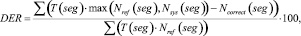 (1)
(1)
где T(seg) – длительность речевого сегмента seg; Nref(seg) – количество дикторов, голос которых присутствует на речевом сегменте seg в соответствии с эталонной разметкой; Nsys(seg) – количество дикторов, голос которых присутствует на речевом сегменте seg в соответствии с результатом работы оцениваемой системы; Ncorrect(seg) – количество верно отнесенных к речевому сегменту seg дикторов.
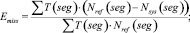
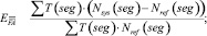 (2)
(2)
 (3)
(3)
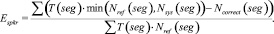 (4)
(4)
Величина DER является суммой трех ошибок: ошибка ложного детектирования речи EFA (2), ошибка ложного пропуска речи Emiss (3) и ошибка разделения дикторов Espkr (4). Автор работы [1] отмечает, что первые два вида ошибок относятся к оценке качества работы систем детектирования речевой активности, третья составляющая используется именно для сравнения систем разделения дикторов. Следует отметить, что, кроме представленной выше методики существуют и другие способы оценки систем диаризации, эффективность которых еще исследуется.
Подготовка и проведение экспериментов
Суть экспериментов заключается в тестировании свободно распространяемых систем разделения дикторов на реальных данных и оценке качества их работы с помощью критерия DER. В качестве тестовых данных для экспериментов использовались шесть аудиофайлов из корпуса NIST2008-ENG: ENG_fabrl.wav, ENG_fadxy.wav, ENG_fafgm.wav, ENG_fafrk.wav, ENG_fagru.wav, ENG_faicw.wav. Формат файлов Wav 16 бит, частота дискретизации 11,025 кГц, для каждого файла имеется текстовый файл с эталонной разметкой в формате RTTM. В связи с тем, что часть систем разделения дикторов требуют использовать файлы с частотой дискретизации 16 кГц, с помощью утилиты ffmpeg исходные аудиофайлы были перекодированы в файлы с частотой дискретизации 16 кГц. В список файлов для тестирования был добавлен еще один аудиофайл формата Wav, для которого в соответствии с рекомендациями NIST [14] был создан специальный файл ключевой разметки.
Для оценки качества работы систем разделения дикторов использовался сценарий на языке Perl md-eval-v21.pl [17], который предоставляется NIST. Он позволяет рассчитывать значения DER на основе двух файлов в формате RTTM, файла эталонной разметки и файла разметки, которую формирует система разделения дикторов. Каждая из рассматриваемых систем разделения дикторов сохраняет результаты своей работы в текстовых файлах своего собственного формата, поэтому были написаны Python сценарии перевода файлов в файлы, соответствующие формату RTTM.
На основе алгоритмов, предложенных автором диссертационной работы [1], разработано платное программное обеспечение, осуществляющее разделение дикторов на фонограмме. После того как мы обратились к автору работы [1], он предоставил нам результаты тестирования своей системы на 6 аудиофайлах корпуса NIST2008-ENG, для сравнения результатов работы свободно распространяемых систем.
Нами было проведено тестирование систем разделения дикторов на файлах из корпуса NIST2008-ENG. Система разделения дикторов на основе LIUM по неустановленным причинам не смогла обработать два аудиофайла: ENG_fadxy.wav, ENG_fagru.wav. В ходе выполнения процесс разделения дикторов зависал и переставал отвечать. Система ELIS некорректно обработала файл, взятый не из корпуса. Произвести тестирование системы DiarTK не удалось. При запуске тестирования она зависала или завершалась с ошибкой. Было написано письмо разработчикам системы с просьбой более подробно описать алгоритм запуска системы и алгоритм подготовки исходных данных для тестирования. Авторы не ответили.
Результаты тестирования представлены в табл. 1. В ней отображены средние значения ошибок для соответствующей системы. Отдельно в табл. 2 вынесены результаты тестирования систем на аудиофайле, взятом не из корпуса.
Таблица 1
Результаты тестирования систем на файлах из корпуса NIST2008-ENG
|
Система |
EFA |
Emiss |
Espkr |
DER |
|
LIUM |
40 |
0,05 |
11,8 |
51,85 |
|
AudioSeg |
47,51 |
0,32 |
41,1 |
88,93 |
|
ELIS |
29,78 |
2,37 |
36,5 |
68,65 |
|
система [1][6] |
8,56 |
39,1 |
2,17 |
49,83 |
Таблица 2
Результаты тестирования систем на файле, взятом не из корпуса
|
Система |
EFA |
Emiss |
Espkr |
DER |
|
LIUM |
18,1 |
0 |
30,6 |
48,7 |
|
AudioSeg |
18,1 |
0 |
82 |
100,1 |
Из табл. 1 и 2 видно, что наименьшую ошибку из протестированных систем дала система разделения дикторов на основе LIUM. По умолчанию система разделения дикторов на основе LIUM использует в качестве акустических признаков 13 MFCC, были проведены опыты с применением различного количества признаков от 13 до 19. В табл. 3 представлены результаты работы системы со стандартным количеством признаков MFCC и результаты, давшие минимальную ошибку.
Таблица 3
Результаты тестирования LIUM с различным количеством MFCC
|
Файл |
MFCC |
EFA |
Emiss |
Espkr |
DER |
|
ENG_fafrk |
13 |
27,7 |
0 |
9,0 |
36,7 |
|
ENG_fafrk |
16 |
27,7 |
0 |
11,6 |
39,3 |
|
ENG_fabrl |
13 |
46,3 |
0 |
23,0 |
69,3 |
|
ENG_fabrl |
14 |
46,3 |
0 |
23,5 |
69,8 |
|
ENG_fafgm |
13 |
33,1 |
0 |
8,7 |
41,8 |
|
ENG_fafgm |
16 |
33,1 |
0 |
6,3 |
39,4 |
|
ENG_faicw |
13 |
52,9 |
0 |
6,5 |
59,4 |
|
ENG_faicw |
17,18,19 |
52,9 |
0 |
3,8 |
56,7 |
|
Файл не из корпуса |
13 |
18,1 |
0 |
30,6 |
48,7 |
|
Файл не из корпуса |
19 |
18,1 |
0 |
19,9 |
38 |
Выводы
Рассмотрены и представлены свободно распространяемые программные продукты для организации систем разделения дикторов. В ходе тестирования наилучшие результаты показали система разделения дикторов, созданная на основе алгоритмов [1], а также система разделения дикторов на основе LIUM. Однако, учитывая, что тестирование систем проводилось с использованием настроек по умолчанию, однозначно выделить наиболее удачные системы разделения дикторов нельзя. Заметим, что суммарная длительность аудиоданных, на которых проводилось тестирование, была недостаточной для окончательных выводов о работоспособности систем – всего 30 минут. Обычно тесты систем проводятся на аудиоданных суммарной длительностью более нескольких часов.
Работа выполнена при финансовой поддержке Программы стратегического развития ПетрГУ в рамках реализации комплекса мероприятий по развитию научно-исследовательской деятельности.
Рецензенты:
Колесников Г.Н., д.т.н., профессор, зав. кафедрой общетехнических дисциплин, Институт лесных, инженерных и строительных наук, Петрозаводский государственный университет, г. Петрозаводск;
Печников А.А., д.т.н., доцент, ведущий научный сотрудник, Институт прикладных математических исследований, Карельский научный центр РАН, г. Петрозаводск.
Библиографическая ссылка
Рогов А.А., Петров Е.А. АНАЛИЗ СУЩЕСТВУЮЩИХ СВОБОДНО РАСПРОСТРАНЯЕМЫХ СИСТЕМ РАЗДЕЛЕНИЯ ДИКТОРОВ НА ФОНОГРАММЕ // Фундаментальные исследования. – 2015. – № 6-1.
– С. 67-72;
URL: https://fundamental-research.ru/ru/article/view?id=38395 (дата обращения: 09.02.2023).
Предлагаем вашему вниманию журналы, издающиеся в издательстве «Академия Естествознания»
(Высокий импакт-фактор РИНЦ, тематика журналов охватывает все научные направления)
Время прочтения
11 мин
Просмотры 8.8K
Привет, Хабр. Я бы хотел рассказать об одном из подходов в решении задачи диаризации дикторов и показать, как этот метод можно реализовать на языке python. Чтобы не отпугивать читателя, я не буду приводить сложные математические формулы (отчасти потому что я и сам «не настоящий сварщик»), а постараюсь изложить всё простым языком и рассказать всё так, чтобы понял разработчик, никогда прежде не сталкивавшийся с машинным обучением.
Готовясь написать эту статью, я выбирал между двумя вариантами изложения: для тех, кто уже знаком с Data Science и тех, кто просто хорошо программирует. В итоге я выбрал второй вариант, решив, что это будет неплохой демонстрацией возможностей DS.
Постановка задачи
Как говорит нам Википедия, диаризация — это процесс разделения входящего аудиопотока на однородные сегменты в соответствии с принадлежностью аудиопотока тому или иному говорящему. Иными словами, запись нужно разделить на кусочки и пронумеровать: вот в этих местах говорит один человек, а вот в этих другой. С точки зрения машинного обучения, подобного рода задачи принадлежат к классу обучения без учителя и называются кластеризацией. О том, какие методы кластеризации существуют можно почитать например здесь или здесь, я же рассажу только о тех, которые нам пригодятся — это Гауссова Смесь Распределений (Gaussian Mixture Model) и Спектральная Кластеризация (Spectral Clustering). Но о них чуть позже.
Начнём с самого начала.
Подготовка окружения
Спойлер
Не был уверен, стоит ли оставлять этот раздел — не хотелось превращать статью в совсем уж туториал. Но в итоге оставил. Кому не нужно, тот пропустит, а тем, кто будет делать всё с нуля, этот шаг облегчит старт.
Вообще говоря, помимо R, язык python является основным при решении задач Data Science, и если вы еще не пробовали программировать на нём, то я очень рекомендую это сделать, потому что python позволяет сделать многие вещи изящно, буквально в несколько строк (кстати, есть даже такой мем).
Существуют две отдельно развивающиеся ветки питона — версии 2 и 3. В моих примерах я использовал версию 3.6, но при желании их легко можно портировать на версию 2.7. Любую из этих веток удобно разворачивать вместе с инсталятором Анаконда, установив который вы сразу же получите интерактивную оболочку для разработки — IPython.
Помимо самой среды разработки понадобятся дополнительные библиотеки: librosa (для работы с аудио и извлечением признаков), webrtcvad (для сегментации) и pickle (для записи обученных моделей в файл). Все они устанавливаются простой командой в Anaconda Prompt
pip install [library]Feature Extraction
Начнём с извлечения признаков — данных, с которыми будут работать модели машинного обучения. В принципе, звуковой сигнал сам по себе — это уже данные, а именно упорядоченный массив значений амплитуды звука, к которому добавляется заголовок, содержащий количество каналов, частоту дискретизации и прочую информацию. Но анализировать эти данные напрямую мы не сможем, поскольку они не содержат таких вещей, глядя на которые, наша модель может сказать — ага, вот эти куски принадлежат одному и тому же человеку.
В задачах обработки речи существует несколько подходов к извлечению признаков. Одним из них является получение мел-частотных кепстральных коэффициентов (Mel Frequency Cepstral Coefficients). О них здесь уже писали, поэтому я лишь слегка напомню.
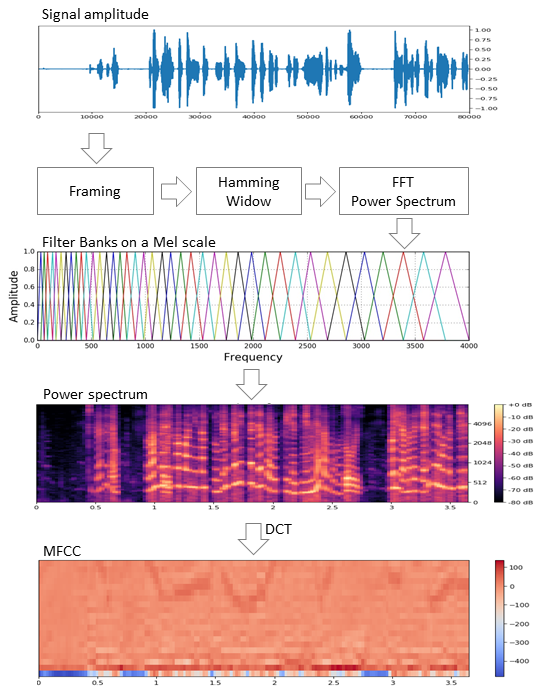
Исходный сигнал нарезают на фреймы длиной 16-40 мс. Далее, применив к фрейму окно Хемминга, делают быстрое преобразование Фурье и получают спектральную плотность мощности. Затем специальной «гребёнкой» фильтров, расположенных равномерно по мел-шкале делают мел-спектрограмму, к которой применяют дискретное косинусное преобразование (DCT) — широко используемый алгоритм сжатия данных. Полученные таким образом коэффициенты представляют из себя некую сжатую характеристику фрейма, при этом, поскольку фильтры, которые мы применяли, расположены были в мел-шкале, коэффициенты несут больше информации в диапазоне восприятия человеческого уха. Как правило, используют от 13 до 25 MFCC на фрейм. Поскольку помимо самого спектра индивидуальность голоса формируется скоростью и ускорениями, MFCC комбинируют с первой и второй производными.
Вообще, MFCC — это самый распространённый вариант работы с речью, но помимо них существуют и другие признаки — LPC (Linear Predictive Coding) и PLP (Perceptual Linear Prediction), а еще иногда можно встретить LFCC, где вместо мел-шкалы используется линейная.
Посмотрим, как извлечь MFCC в python.
import numpy as np
import librosa
mfcc=librosa.feature.mfcc(y=y, sr=sr,
                          hop_length=int(hop_seconds*sr),
                          n_fft=int(window_seconds*sr),
                          n_mfcc=n_mfcc)
mfcc_delta=librosa.feature.delta(mfcc)
mfcc_delta2=librosa.feature.delta(mfcc, order=2)
stacked=np.vstack((mfcc, mfcc_delta, mfcc_delta2))
features=stacked.T #librosa возвращает где MFCC идут в ряд, а для модели нужно будет в столбец.
Как видим, делается это действительно всего в несколько строк. Теперь перейдём к первому алгоритму кластеризации.
Gaussian Mixture Model
Модель смеси Гауссовых распределений предполагает что наши данные — это смесь многомерных распределений Гаусса с определёнными параметрами.
При желании можно легко найти и детальное описание модели и как работает EM-алгоритм, обучающий эту модель, я же обещал не наводить тоску сложными формулами и поэтому покажу красивые примеры из этой статьи.
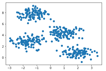
Сгенерируем четыре кластера и нарисуем их.
from sklearn.datasets.samples_generator import make_blobs
X, y_true=make_blobs(n_samples=400, centers=4,
                       cluster_std=0.60, random_state=0)
plt.scatter(X[:, 0], X[:, 1]);
Создадим модель, обучим на наших данных и снова отрисуем точки но уже с учётом предсказанной моделью принадлежности к кластерам.
from sklearn.mixture import GaussianMixture
gmm = GaussianMixture(n_components=4)
gmm.fit(X)
labels=gmm.predict(X)
plt.scatter(X[:, 0], X[:, 1], c=labels, s=40, cmap='viridis');
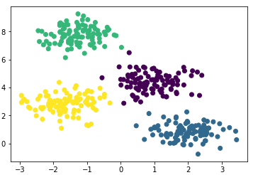
Модель неплохо справилась с искусственными данными. В принципе, регулируя число компонент смеси и тип матрицы ковариаций (число степеней свободы гауссиан), можно описывать достаточно сложные данные.
Итак, мы знаем как делать параметризацию данных и умеем обучать модель смеси гауссовых распределений. Теперь можно было бы попробовать сделать кластеризацию в лоб — обучая GMM на извлеченных из диалога MFCC. И, наверное, в каком-то идеальном сферически-вакуумном диалоге, в котором каждый диктор будет укладываться в свою гауссиану, мы получим хороший результат. Понятное дело, что в реальности такого никогда не будет. На самом деле с помощью GMM моделируют не диалог, а каждого человека в диалоге — т. е. представляют, что голос каждого диктора в извлечённых признаках описывается своим набором гауссиан.
Подытоживая, мы потихоньку подбираемся к основной теме.
Сегментация
Традиционно процесс диаризации состоит из трёх последовательных блоков — обнаружение речи (Voice Activity Detection), сегментация и кластеризация (есть модели, в которых последние два шага совмещены, см. LIA E-HMM).
В первом шаге происходит отделение речи от различного рода шумов. Алгоритм VAD определяет является ли поданный на него кусок аудиозаписи речью, или это, например, звучит сирена или кто-то чихнул. Понятное дело, что для того, чтобы такой алгоритм был качественным необходимо обучение с учителем. А это в свою очередь означает, что необходимо размечать данные — иными словами создавать базу данных с записями речи и всевозможных шумов. Мы поступим лениво — возьмём готовый VAD, который работает не идеально, но для начала нам хватит.
Второй блок нарезает данные с речью на сегменты с одним активным говорящим. Классическим подходом в этом плане является алгоритм определения смены диктора на основе байесовского информационного критерия — BIC. Суть этого метода заключается в следующем — скользящим окном проходятся по аудиозаписи и в каждой точке прохода отвечают на вопрос: «Как данные в этом месте лучше описываются — одним распределением или двумя?». Для ответа на этот вопрос вычисляется параметр  , исходя из знака которого принимается решение о смене диктора. Проблема в том, что этот метод будет работать не очень хорошо в случае частой смены диктора, да еще в присутствии шумов (которые очень характерны для записи телефонного разговора).
Небольшое пояснение
В оригинале я работал с записями телефонных разговоров кол-центра средней продолжительностью около 4-х минут. По понятным причинам эти записи я выложить не могу, поэтому для демонстрации я взял запись интервью с одной радиостанции. В случае с длинным интервью этот метод возможно дал бы приемлемый результат, но на моих данных он не сработал.
В условиях, когда дикторы друг друга не перебивают, и их голоса не накладываются друг на друга, VAD, который мы будем использовать, более менее справляется с задачей сегментации, поэтому первые два шага у нас будут выглядеть следующим образом.
#читаем сигнал
y_, sr = librosa.load('data/2018-08-26-beseda-1616.mp3', sr=SR)
#первым шагом делаем pre-emphasis: усиление высоких частот
pre_emphasis = 0.97
y = np.append(y[0], y[1:] - pre_emphasis * y[:-1])

#все что ниже фактически взято с гитхаба webrtcvad с небольшими изменениями
vad = webrtcvad.Vad(2) # агрессивность VAD
audio = np.int16(y/np.max(np.abs(y)) * 32767)

frames = frame_generator(10, audio, sr)
frames = list(frames)
segments = vad_collector(sr, 50, 200, vad, frames)

if not os.path.exists('data/chunks'): os.makedirs('data/chunks')
for i, segment in enumerate(segments):
    chunk_name = 'data/chunks/chunk-%003d.wav' % (i,)
    # vad добавляет в конце небольшой кусочек тишины, который нам не нужен
    write_wave(chunk_name, segment[0: len(segment)-int(100*sr/1000)], sr)
В действительности люди конечно будут говорить одновременно. Более того, VAD в некоторых местах сплоховал, из-за того, что запись не живая, а представляет собой склейку, в которой вырезаны паузы. Вы можете попробовать повторить нарезку на сегменты, увеличив агрессивность VAD’а с 2-х до 3-х.
GMM-UBM
Теперь у нас есть отдельные сегменты, и мы решили, что будем с помощью GMM моделировать каждого диктора. Извлечём признаки из сегмента и на этих данных обучим модель. Сделаем так на каждом сегменте и получившиеся модели сравним между собой. Вполне оправдано ожидать, что модели, обученные на сегментах, принадлежащих одному и тому же человеку, будут как-то схожи. Но тут мы сталкиваемся со следующей проблемой, извлекая признаки из аудиофайла длиной 1 сек с частотой дискретизации 8000 Гц при размере окна 10 мс, мы получим набор из 800 векторов MFCC. На таких данных наша модель обучиться не сможет, потому что это ничтожно мало. Даже, если это будет не одна секунда, а десять, данных все равно будет недостаточно. И здесь на помощь приходит Универсальная Фоновая Модель (UBM — Universal Background Model), её еще называют дикторонезависимой. Идея заключается в следующем. Мы обучим GMM на большой выборке данных (в нашем случае это полная запись интервью) и получим на выходе акустическую модель обобщённого диктора (это и будем наша UBM). А затем, используя специальный алгоритм адаптации (о нём чуть ниже), мы будем «подгонять» эту модель под признаки, извлекаемые из каждого сегмента. Этот подход широко используется не только для диаризации, но и в системах распознавания по голосу. Для распознания человека по голосу сначала нужно обучить модель на нём и без UBM нужно было бы иметь в распоряжении по несколько часов записи речи этого человека.
Из каждой адаптированной GMM мы извлечём вектор коэффициентов сдвига  (он же медиана или мат. ожидание, если угодно) и, основываясь, на данных об этих векторах со всех сегментов, будем делать кластеризацию (ниже будет понятно почему именно вектор сдвигов).
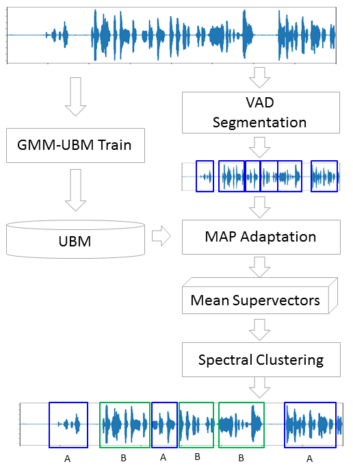
MAP Adaptation
Метод, которым мы будем подгонять UBM под каждый сегмент называется Maximum A-Posteriori Adaptation. В общем случае алгоритм следующий. Сначала рассчитывается апостериорная вероятность на адаптационных данных и достаточные статистики для веса, медианы и дисперсии каждой гауссианы. Затем полученные статистики комбинируются с параметрами UBM и получаются параметры адаптированной модели. В нашем случае мы будем адаптировать только медианы, не затрагивая остальных параметров. Не смотря на то, что обещал не углубляться в математику, приведу всё-таки три формулы, потому что MAP адаптация — ключевой момент в этой статье.


Здесь  — апостериорная вероятность,
  — достаточная статистика для ,
  — медиана адаптированной модели,
  — коэффициент адаптации,
  — фактор соответствия.
Если все это кажется белибердой и вызывает уныние — не отчаивайтесь. На самом деле для понимания работы алгоритма необязательно вникать в эти формулы, его работу легко можно продемонстрировать следующим примером:

Допустим у нас есть какие-то достаточно большие данные, и мы обучили на них UBM (левый рисунок, UBM — это двухкомпонентная смесь гауссовых распределений). Появляются новые данные, которые не укладываются в нашу модель (рисунок посередине). С помощью указанного алгоритма мы будем смещать центры гауссиан так, чтобы они ложились на новые данные (рисунок справа). Применяя этот алгоритм на экспериментальных данных, мы будем ожидать, что на сегментах с одним и тем же диктором гауссианы будут смещаться в одном направлении, образуя таким образом кластеры. Именно поэтому для кластеризации сегментов мы будем использовать данные о сдвиге .
Итак, давайте проведём MAP адаптацию для каждого сегмента. (Для справки: помимо MAP Adaptation широко используется метод MLLR — Maximum Likelihood Linear Regression и некоторые его модификации. Также пробуют эти два метода объединять.)
SV = []

# возьмём сегменты от chunk-000 до chunk-100
for i in range(101):
    clear_output(wait=True)
    fname='data/chunks/chunk-%003d.wav' % (i,)
    print('UBM MAP adaptation for {0}'.format(fname))
    y_, sr_ = librosa.load(fname, sr=None)
    f_ = extract_features(y_, sr_, window=N_FFT, hop=HOP_LENGTH, n_mfcc=N_MFCC)
    f_ = preprocessing.scale(f_)
    gmm = copy.deepcopy(ubm)
    gmm = map_adaptation(gmm, f_, max_iterations=1, relevance_factor=16)
    sv = gmm.means_.flatten() #получаем супервектор мю
    sv = preprocessing.scale(sv)
    SV.append(sv)
SV = np.array(SV)
clear_output()
print(SV.shape)
Теперь, когда для каждого сегмента у нас есть данные о , мы наконец переходим к финальному шагу.
Спектральная кластеризация
Спектральная кластеризация вкратце описана в статье, ссылку на которую я приводил в самом начале. Алгоритм строит полный граф, где вершины — это наши данные, а рёбра между ними — это мера схожести. В задачах распознавания голоса в качестве такой меры используется косинусная метрика, поскольку она учитывает угол между векторами, игнорируя их магнитуду (которая не несёт информации о дикторе). Построив граф, рассчитываются собственные векторы матрицы Кирхгофа (которая по сути является представлением полученного графа) и затем применяется какой-нибудь стандартный метод кластеризации, например метод k-средних. Укладывается всё это в две строчки кода
N_CLUSTERS = 2
sc = SpectralClustering(n_clusters=N_CLUSTERS, affinity='cosine')
labels = sc.fit_predict(SV) # кластеры могут быть не упорядочены, напр. [2,1,1,0,2]
labels = rearrange(labels, N_CLUSTERS) # эта функция упорядочивает кластеры [0,1,1,2,0]
print(labels)
# глядя на результат, понимаем, что 1 - это интервьюер. выведем все номера сегментов
print([i for i, x in enumerate(labels) if x == 1])
Выводы и дальнейшие планы
Описанный алгоритм был опробован с различными параметрами:
- Количество MFCC: 7, 13, 20
- MFCC в комбинации с LPC
- Тип и количество смесей в GMM: full [8, 16, 32], diag [8, 16, 32, 64, 256]
- Методы адаптации UBM: MAP (с covariance_type = ‘full’) и MLLR (с covariance_type = ‘diag’)
В итоге, субъективно оптимальным остались параметры: MFCC 13, GMM covariance_type = ‘full’ n_components = 16.
К сожалению, у меня не хватило терпения (эту статью я начал писать больше месяца назад) для того, чтобы разметить полученные сегменты и посчитать DER (Diariztion Error Rate). Субъективно работу алгоритма я оцениваю как «в принципе неплохо, но далеко от идеала». Сделав кластеризацию на векторах, полученных из первой сотни сегментов (с одним проходом MAP), а затем выделив те, где говорит интервьюер (девушка, она там говорит гораздо меньше гостя), кластеризация выдаёт список ![$[1, 2, 25, 26, 46, 48, 49, 61, 85, 86]$](https://habrastorage.org/getpro/habr/formulas/b5f/5b8/c96/b5f5b8c962e564d107227d8156c32384.svg) , что является 100% попаданием. При этом выпадают сегменты, где присутствуют оба диктора (например 14), но это уже можно свалить на ошибку VAD’а. Причём такие сегменты начинают учитываться с увеличением числа проходов MAP. Важный момент. Интервью, с которым мы работали — более менее «чистое». Если добавляются различные музыкальные вставки, шумы и прочие неречевые штуки, кластеризация начинает хромать. Поэтому в планах попробовать обучить собственный VAD (потому что webrtcvad, например, не отделяет музыку от речи).
, что является 100% попаданием. При этом выпадают сегменты, где присутствуют оба диктора (например 14), но это уже можно свалить на ошибку VAD’а. Причём такие сегменты начинают учитываться с увеличением числа проходов MAP. Важный момент. Интервью, с которым мы работали — более менее «чистое». Если добавляются различные музыкальные вставки, шумы и прочие неречевые штуки, кластеризация начинает хромать. Поэтому в планах попробовать обучить собственный VAD (потому что webrtcvad, например, не отделяет музыку от речи).
В связи с тем, что изначально я работал с телефонным разговором, у меня не было необходимости оценивать количество дикторов. Но не всегда количество дикторов предопределено, даже если это интервью. Например в этом интервью в середине звучит анонс, наложенный на музыку, и озвученный дополнительными двумя людьми. Поэтому интересно было бы попробовать метод оценки количества дикторов, указанный в первой статье в разделе списка литературы (основанный на анализе собственных значений нормализованной матрицы Лапласа).
Список литературы
Помимо материалов, расположенных по ссылкам в тексте и Jupyter ноутбуках, для подготовки этой статьи были использованы следующие источники:
- Speaker Diarization using GMM Supervector and Advanced Reduction Algorithms. Nurit Spingarn
- Feature Extraction Methods LPC, PLP and MFCC In Speech Recognition. Namrata Dave
- MAP estimation for mulivariate gaussian mixture observations of markov chains. Jean-Luc Gauvain and Chin-Hui Lee
- On Spectral Clustering Analysis and an algorithm. Andrew Y. Ng, Michael I. Jordan, Yair Weiss
- Speaker recognition using universal background model on YOHO database. Alexandre Majetniak
Добавлю также некоторые проекты по диаризации:
- Sidekit и расширение для диаризации s4d. Библиотека на python для работы с речью. К сожалению, документация оставляет желать лучшего.
- Bob и разные её части как например bob.bio, bob.learn.em — библиотека на python для обработки сигнала и работы с биометрическими данными. Windows не поддерживается.
- LIUM — готовое решение, написанное на Java.
Весь код выложен на гитхабе. Для удобства я сделал несколько Jupyter ноутбуков с демонстрацией отдельных вещей — MFCC, GMM, MAP Adaptation и Diarization. В последнем находится основной процесс. Также в репозитории pickle-файлы с некоторыми предобученными моделями и само интервью.
I. Overview
This suite supports evaluation of diarization system output relative
to a reference diarization subject to the following conditions:
- both the reference and system diarizations are saved within Rich
Transcription Time Marked (RTTM) files - for any pair of recordings, the sets of speakers are disjoint
II. Dependencies
The following Python packages are required to run this software:
- Python >= 2.7.1* (https://www.python.org/)
- NumPy >= 1.6.1 (https://github.com/numpy/numpy)
- SciPy >= 0.17.0 (https://github.com/scipy/scipy)
- intervaltree >= 3.0.0 (https://pypi.python.org/pypi/intervaltree)
- tabulate >= 0.5.0 (https://pypi.python.org/pypi/tabulate)
- Tested with Python 2.7.X, 3.6.X, and 3.7.X.
III. Metrics
Diarization error rate
Following tradition in this area, we report diarization error rate (DER), which
is the sum of
- speaker error — percentage of scored time for which the wrong speaker id
is assigned within a speech region - false alarm speech — percentage of scored time for which a nonspeech
region is incorrectly marked as containing speech - missed speech — percentage of scored time for which a speech region is
incorrectly marked as not containing speech
As with word error rate, a score of zero indicates perfect performance and
higher scores (which may exceed 100) indicate poorer performance. For more
details, consult section 6.1 of the NIST RT-09 evaluation plan.
Jaccard error rate
We also report Jaccard error rate (JER), a metric introduced for DIHARD II that is based on the Jaccard index. The Jaccard index is a similarity
measure typically used to evaluate the output of image segmentation systems and
is defined as the ratio between the intersection and union of two segmentations.
To compute Jaccard error rate, an optimal mapping between reference and system
speakers is determined and for each pair the Jaccard index of their
segmentations is computed. The Jaccard error rate is then 1 minus the average
of these scores.
More concretely, assume we have N reference speakers and M system
speakers. An optimal mapping between speakers is determined using the
Hungarian algorithm so that each reference speaker is paired with at most one
system speaker and each system speaker with at most one reference speaker. Then,
for each reference speaker ref the speaker-specific Jaccard error rate is
(FA + MISS)/TOTAL, where:
TOTALis the duration of the union of reference and system speaker
segments; if the reference speaker was not paired with a system speaker, it is
the duration of all reference speaker segmentsFAis the total system speaker time not attributed to the reference
speaker; if the reference speaker was not paired with a system speaker, it is
0MISSis the total reference speaker time not attributed to the system
speaker; if the reference speaker was not paired with a system speaker, it is
equal toTOTAL
The Jaccard error rate then is the average of the speaker specific Jaccard error
rates.
JER and DER are highly correlated with JER typically being higher, especially in
recordings where one or more speakers is particularly dominant. Where it tends
to track DER is in outliers where the diarization is especially bad, resulting
in one or more unmapped system speakers whose speech is not then penalized. In
these cases, where DER can easily exceed 500%, JER will never exceed 100% and
may be far lower if the reference speakers are handled correctly. For this
reason, it may be useful to pair JER with another metric evaluating speech
detection and/or speaker overlap detection.
Clustering metrics
A third approach to system evaluation is convert both the reference and system
outputs to frame-level labels, then evaluate using one of many well-known
approaches for evaluating clustering performance. Each recording is converted to
a sequence of 10 ms frames, each of which is assigned a single label
corresponding to one of the following cases:
- the frame contains no speech
- the frame contains speech from a single speaker (one label per speaker
indentified) - the frame contains overlapping speech (one label for each element in the
powerset of speakers)
These frame-level labelings are then scored with the following metrics:
Goodman-Kruskal tau
Goodman-Kruskal tau is an asymmetric association measure dating back to work
by Leo Goodman and William Kruskal in the 1950s (Goodman and Kruskal, 1954).
For a reference labeling ref and a system labeling sys,
GKT(ref, sys) corresponds to the fraction of variability in sys that
can be explained by ref. Consequently, GKT(ref, sys) is 1 when ref
is perfectly predictive of sys and 0 when it is not predictive at all.
Correspondingly, GKT(sys, ref) is 1 when sys is perfectly predictive
of ref and 0 when lacking any predictive power.
B-cubed precision, recall, and F1
The B-cubed precision for a single frame assigned speaker S in the
reference diarization and C in the system diarization is the proportion of
frames assigned C that are also assigned S. Similarly, the B-cubed
recall for a frame is the proportion of all frames assigned S that are
also assigned C. The overall precision and recall, then, are just the mean
of the frame-level precision and recall measures and the overall F-1 their
harmonic mean. For additional details see Bagga and Baldwin (1998).
Information theoretic measures
We report four information theoretic measures:
H(ref|sys)— conditional conditional entropy in bits of the reference
labeling given the system labelingH(sys|ref)— conditional conditional entropy in bits of the system
labeling given the reference labelingMI— mutual information in bits between the reference and system
labelingsNMI— normalized mutual information between the reference and system
labelings; that is,MIscaled to the interval [0, 1]. In this case, the
normalization term used issqrt(H(ref)*H(sys)).
H(ref|sys) is the number of bits needed to describe the reference
labeling given that the system labeling is known and ranges from 0 in
the case that the system labeling is perfectly predictive of the reference
labeling to H(ref) in the case that the system labeling is not at
all predictive of the reference labeling. Similarly, H(sys|ref) measure
the number of bits required to describe the system labeling given the
reference labeling and ranges from 0 to H(sys).
MI is the number of bits shared by the reference and system labeling and
indicates the degree to which knowing either reduces uncertainty in the other.
It is related to conditional entropy and entropy as follows:
MI(ref, sys) = H(ref) - H(ref|sys) = H(sys) - H(sys|ref). NMI is
derived from MI by normalizing it to the interval [0, 1]. Multiple
normalizations are possible depending on the upper-bound for MI that is
used, but we report NMI normalized by sqrt(H(ref)*H(sys)).
IV. Scoring
To evaluate system output stored in RTTM files sys1.rttm,
sys2.rttm, … against a corresponding reference diarization stored in RTTM
files ref1.rttm, ref2.rttm, …:
python score.py -r ref1.rttm ref2.rttm ... -s sys1.rttm sys2.rttm ...
which will calculate and report the following metrics both overall and on
a per-file basis:
DER— diarization error rate (in percent)JER— Jaccard error rate (in percent)B3-Precision— B-cubed precisionB3-Recall— B-cubed recallB3-F1— B-cubed F1GKT(ref, sys)— Goodman-Kruskal tau in the direction of the reference
diarization to the system diarizationGKT(sys, ref)— Goodman-Kruskal tau in the direction of the system
diarization to the reference diarizationH(ref|sys)— conditional entropy in bits of the reference diarization
given the system diarizationH(sys|ref)— conditional entropy in bits of the system diarization
given the reference diarizationMI— mutual information in bitsNMI— normalized mutual information
Alternately, we could have specified the reference and system RTTM files via
script files of paths (one per line) using the -R and -S flags:
python score.py -R ref.scp -S sys.scp
By default the scoring regions for each file will be determined automatically
from the reference and speaker turns. However, it is possible to specify
explicit scoring regions using a NIST un-partitioned evaluation map (UEM) file and the -u flag. For instance, the following:
python score.py -u all.uem -R ref.scp -S sys.scp
will load the files to be scored plus scoring regions from all.uem, filter
out and warn about any speaker turns not present in those files, and trim the
remaining turns to the relevant scoring regions before computing the metrics
as before.
DER is scored using the NIST md-eval.pl tool with a default collar size of
0 ms and explicitly including regions that contain overlapping speech in the
reference diarization. If desired, this behavior can be altered using the
--collar and --ignore_overlaps flags. For instance
python score.py --collar 0.100 --ignore_overlaps -R ref.scp -S sys.scp
would compute DER using a 100 ms collar and with overlapped speech ignored.
All other metrics are computed off of frame-level labelings generated from the
reference and system speaker turns WITHOUT any use of collars. The default
frame step is 10 ms, which may be altered via the --step flag. For more
details, consult the docstrings within the scorelib.metrics module.
The overall and per-file results will be printed to STDOUT as a table; for
instance:
File                           DER    JER    B3-Precision    B3-Recall    B3-F1    GKT(ref, sys)    GKT(sys, ref)    H(ref|sys)    H(sys|ref)    MI    NMI
---------------------------  -----  -----  --------------  -----------  -------  ---------------  ---------------  ------------  ------------  ----  -----
CMU_20020319-1400_d01_NONE    6.10  20.10            0.91         1.00     0.95             1.00             0.88          0.22          0.00  2.66   0.96
ICSI_20000807-1000_d05_NONE  17.37  21.92            0.72         1.00     0.84             1.00             0.68          0.65          0.00  2.79   0.90
ICSI_20011030-1030_d02_NONE  13.06  25.61            0.80         0.95     0.87             0.95             0.80          0.54          0.11  5.10   0.94
LDC_20011116-1400_d06_NONE    5.64  16.10            0.95         0.89     0.92             0.85             0.93          0.10          0.27  1.87   0.91
LDC_20011116-1500_d07_NONE    1.69   2.00            0.96         0.96     0.96             0.95             0.95          0.14          0.12  2.39   0.95
NIST_20020305-1007_d01_NONE  42.05  53.38            0.51         0.95     0.66             0.93             0.44          1.58          0.11  2.13   0.74
*** OVERALL ***              14.31  26.75            0.81         0.96     0.88             0.96             0.80          0.55          0.10  5.45   0.94
Some basic control of the formatting of this table is possible via the
--n_digits and --table_format flags. The former controls the number of
decimal places printed for floating point numbers, while the latter controls
the table format. For a list of valid table formats plus example outputs,
consult the documentation for the tabulate package.
For additional details consult the docstring of score.py.
V. File formats
RTTM
Rich Transcription Time Marked (RTTM) files are space-delimited text files
containing one turn per line, each line containing ten fields:
Type— segment type; should always bySPEAKERFile ID— file name; basename of the recording minus extension (e.g.,
rec1_a)Channel ID— channel (1-indexed) that turn is on; should always be
1Turn Onset— onset of turn in seconds from beginning of recordingTurn Duration— duration of turn in secondsOrthography Field— should always by<NA>Speaker Type— should always be<NA>Speaker Name— name of speaker of turn; should be unique within scope
of each fileConfidence Score— system confidence (probability) that information
is correct; should always be<NA>Signal Lookahead Time— should always be<NA>
For instance:
SPEAKER CMU_20020319-1400_d01_NONE 1 130.430000 2.350 <NA> <NA> juliet <NA> <NA>
SPEAKER CMU_20020319-1400_d01_NONE 1 157.610000 3.060 <NA> <NA> tbc <NA> <NA>
SPEAKER CMU_20020319-1400_d01_NONE 1 130.490000 0.450 <NA> <NA> chek <NA> <NA>
If you would like to confirm that a set of RTTM files are valid, use the
included validate_rttm.py script. For instance, if you have RTTMs
fn1.rttm, fn2.rttm, …, then
python validate_rttm.py fn1.rttm fn2.rttm ...
will iterate over each line of each file and warn on any that do not match the
spec.
UEM
Un-partitioned evaluation map (UEM) files are used to specify the scoring
regions within each recording. For each scoring region, the UEM file contains
a line with the following four space-delimited fields
File ID— file name; basename of the recording minus extension (e.g.,
rec1_a)Channel ID— channel (1-indexed) that scoring region is on; ignored by
score.pyOnset— onset of scoring region in seconds from beginning of recordingOffset— offset of scoring region in seconds from beginning of
recording
For instance:
CMU_20020319-1400_d01_NONE 1 125.000000 727.090000
CMU_20020320-1500_d01_NONE 1 111.700000 615.330000
ICSI_20010208-1430_d05_NONE 1 97.440000 697.290000
VI. References
- Bagga, A. and Baldwin, B. (1998). «Algorithms for scoring coreference
chains.» Proceedings of LREC 1998. - Cover, T.M. and Thomas, J.A. (1991). Elements of Information Theory.
- Goodman, L.A. and Kruskal, W.H. (1954). «Measures of association for
cross classifications.» Journal of the American Statistical Association. - NIST. (2009). The 2009 (RT-09) Rich Transcription Meeting Recognition
Evaluation Plan. https://web.archive.org/web/20100606041157if_/http://www.itl.nist.gov/iad/mig/tests/rt/2009/docs/rt09-meeting-eval-plan-v2.pdf - Nguyen, X.V., Epps, J., and Bailey, J. (2010). «Information theoretic
measures for clustering comparison: Variants, properties, normalization
and correction for chance.» Journal of Machine Learning Research. - Pearson, R. (2016). GoodmanKruskal: Association Analysis for Categorical
Variables. https://CRAN.R-project.org/package=GoodmanKruskal. - Rosenberg, A. and Hirschberg, J. (2007). «V-Measure: A conditional
entropy-based external cluster evaluation measure.» Proceedings of
EMNLP 2007. - Strehl, A. and Ghosh, J. (2002). «Cluster ensembles — A knowledge
reuse framework for combining multiple partitions.» Journal of Machine
Learning Research.
Project description
Overview
This is a lightweight library to compute Diarization Error Rate (DER).
Features NOT supported:
- Handling overlapped speech, i.e. two speakers speaking at the same time.
- Allowing segment boundary tolerance, a.k.a. the
collarvalue.
For more sophisticated metrics with these supports, please use
pyannote-metrics instead.
To learn more about speaker diarization, here is a curated list of resources:
awesome-diarization.
Diarization Error Rate
Diarization Error Rate (DER) is the most commonly used metrics for
speaker diarization.
Its strict form is:
       False Alarm + Miss + Overlap + Confusion
DER = ------------------------------------------
                   Reference Length
The definition of each term:
Reference Length:The total length of the reference (ground truth).False Alarm: Length of segments which are considered as speech in
hypothesis, but not in reference.Miss: Length of segments which are considered as speech in
reference, but not in hypothesis.Overlap: Length of segments which are considered as overlapped speech
in hypothesis, but not in reference.
This library does NOT support overlap.Confusion: Length of segments which are assigned to different speakers
in hypothesis and reference (after applying an optimal assignment).
The unit of each term is seconds.
Note that DER can theoretically be larger than 1.0.
References:
- pyannote-metrics documentation
- Xavier Anguera’s thesis
Tutorial
Install
Install the package by:
pip3 install simpleder
or
python3 -m pip install simpleder
API
Here is a minimal example:
import simpleder

# reference (ground truth)
ref = [("A", 0.0, 1.0),
       ("B", 1.0, 1.5),
       ("A", 1.6, 2.1)]

# hypothesis (diarization result from your algorithm)
hyp = [("1", 0.0, 0.8),
       ("2", 0.8, 1.4),
       ("3", 1.5, 1.8),
       ("1", 1.8, 2.0)]

error = simpleder.DER(ref, hyp)

print("DER={:.3f}".format(error))
This should output:
DER=0.350
Download files
Download the file for your platform. If you’re not sure which to choose, learn more about installing packages.
Source Distribution
Built Distribution
1. Introduction to Speaker Diarization
Speaker diarization is the process of segmenting and clustering a speech recording into homogeneous regions and answers the question “who spoke when” without any prior knowledge about the speakers. A typical diarization system performs three basic tasks. Firstly, it discriminates speech segments from the non-speech ones. Secondly, it detects speaker change points to segment the audio data. Finally, it groups these segmented regions into speaker homogeneous clusters.
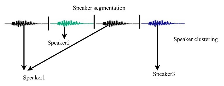
An overview of a speaker diarization system.
Although there are many different approaches to perform speaker diarization, most of them follow the following scheme:
Feature extraction: It extracts specific information from the audio signal and allows subsequent speaker modeling and classification. The extracted features should ideally maximize inter-speaker variability and minimize intra-speaker variability, and represent the relevant information.
Speaker segmentation: It partitions the audio data into acoustically homogeneous segments according to speaker identities. It detects all boundary locations within each speech region that corresponds to speaker change points which are subsequently used for speaker clustering.
Speaker clustering: Speaker clustering groups speech segments that belong to a particular speaker. It has two major categories based on its processing requirements. Its two main categories are online and offline speaker clustering. In the former, speech segments are merged or split in consecutive iterations until the optimum number of speakers is acquired. Since the entire speech file is available before decision making in the later, it provides better results more than the online speaker clustering. The most widely used and popular technique for speaker clustering is Agglomerative Hierarchical Clustering (AHC). AHC builds a hierarchy of clusters, that shows the relations between speech segments, and merges speech segments based on similarity. AHC approaches can be classified into bottom-up and top-down clustering.
Two items need to be defined in both bottom-up and top-down clustering:
1. A distance between speech segments to determine acoustic similarity. The distance metric is used to decide whether or not two clusters must be merged (bottom-up clustering) or split (top-down clustering).
2. A stopping criterion to determine when the optimal number of clusters (speakers) is reached.
Bottom-up (Agglomerative): It starts from a large number of speech segments and merges the closest speech segments iteratively until a stopping criterion is met. This technique is the most widely used in speaker diarization since it is directly applied on the output of speech segments from speaker segmentation. A matrix of distances between every possible pair of clusters is computed and the pair with highest BIC value is merged. Then, the merged clusters are removed from the distance matrix. Finally, the distance matrix table is updated using the distances between the new merged cluster and all remaining clusters. This process is done iteratively until the stopping criterion is met or all pairs have a BIC value less than zero .
Top-down: Top-down Hierarchical Clustering methods start from a small number of clusters, usually a single cluster that contains several speech segments, and the initial clusters are split iteratively until a stopping criterion is met. It is not as widely used as the bottom-up clustering.
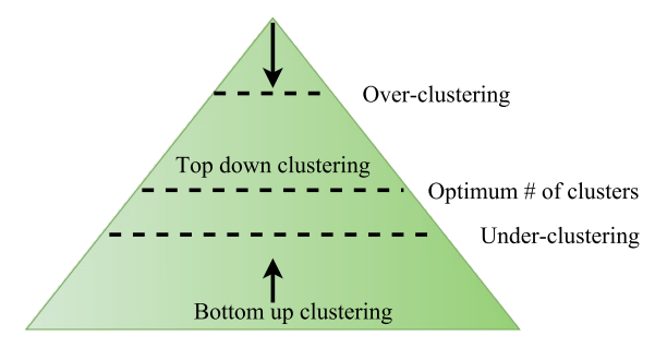
Bottom-Up and Top-down approaches to clustering
2. Approaches to Speaker Diarization
This section describes some of the state-of-the-art speaker diarization systems.
HMM/GMM based speaker diarization system: Each speaker is represented by a state of an HMM and the state emission probabilities are modeled using GMMs. The initial clustering is performed initially by partitioning the audio signal equally which generates a set of segments {
( s_i )
}. Let
( c_i )
represent
( i^{th} )
speaker cluster,
( b_i )
represent the emission probability of cluster
( c_i )
and
( f_t )
denote a given feature vector at time
( t )
. Then, the log-likelihood
( logb_i(s_t) )
of the feature ft for cluster
( c_i )
is calculated as follows:
[ logb_i(s_t)=log sum_{(r)} {w}^r_i N (f_i,{mu}^r_i,sum_{(i)}^r) ]
where
( N() )
is a Gaussian pdf and
( {w}^r_i, {mu}^r_i,sum_{(i)}^r) )
are the weights, means and covariance matrices of the
( r^{th} )
Gaussian mixture component of cluster
( c_i )
, respectively.
The agglomerative hierarchical clustering starts by overestimating the number of clusters. At each iteration, the clusters that are most similar are merged based on the BIC distance. The distance measure is based on modified delta Bayesian information criterion [Ajmera and Wooters, 2003]. The modified BIC distance does not take into account the penalty term that corresponds to the number of free parameters of a multivariate Gaussian distribution and is expressed as:
[ Delta BIC (c_i,c_j)= log sum_{f_t in ( {ci ; cup ; c_j})} log b_{ij}(f_t) — log sum_{f_t in ci} log b_{i}(f_t) — log sum_{f_t in cj} log b_{j}(f_t) ]
where
( b_{ij} )
is the probability distribution of the combined clusters
( c_i )
and
( c_j. )
The clusters that produce the highest BIC score are merged at each iteration. A minimum duration of speech segments is normally constrained for each class to prevent decoding short segments. The number of clusters is reduced at each iteration. When the maximum
( Delta BIC )
distance among these clusters is less than threshold value 0, the speaker diarization system stops and outputs the hypothesis.
Factor analysis techniques: Factor analysis techniques which are the state of the art in speaker recognition have recently been successfully used in speaker diarization. The speech clusters are first represented by i-vectors and the successive clustering stages are performed based on i-vector modeling. The use of factor analysis technique to model speech segments reduces the dimension of the feature vector by retaining most of the relevant information. Once the speech clusters are represented by i-vectors, cosine-distance and PLDA scoring techniques can be applied to decide if two clusters belong to the same or different speaker(s).
Deep learning approaches: Speaker diarization is crucial for many speech technologies in the presence of multiple speakers, but most of the current methods that employ i-vector clustering for short segments of speech are potentially too cumbersome and costly for the front-end role. Thus, it has been proposed by Daniel Povey an alternative approach for learning representations via deep neural networks to remove the i-vector extraction process from the pipeline entirely. The proposed architecture simultaneously learns a fixed-dimensional embedding for acoustic segments of variable length and a scoring function for measuring the likelihood that the segments originated from the same or different speakers. The proposed neural based system matches or exceeds the performance of state-of-the-art baselines.
3. Evaluation Metrics
Diarization Error Rate (DER) is the metric used to measure the performance of speaker diarization systems. It is measured as the fraction of time that is not attributed correctly to a speaker or non-speech.
The DER is composed of the following three errors:
Speaker Error: It is the percentage of scored time that a speaker ID is assigned to the wrong speaker. Speaker error is mainly a diarization system error (i.e., it is not related to speech/non-speech detection.) It also does not take into account the overlap speeches not detected.
False Alarm: It is the percentage of scored time that a hypothesized speaker is labelled as a non-speech in the reference. The false alarm error occurs mainly due to the the speech/non-speech detection error (i.e., the speech/non-speech detection considers a non-speech segment as a speech segment). Hence, false alarm error is not related to segmentation and clustering errors.
Missed Speech: It is the percentage of scored time that a hypothesized non-speech segment corresponds to a reference speaker segment. The missed speech occurs mainly due to the the speech/non-speech detection error (i.e., the speech segment is considered as a non-speech segment). Hence, missed speech is not related to segmentation and clustering errors.
[ DER = Speaker ; Error + False ; Alarm + Miss ; Speech ]