Дизерпанк — статья о дизеринге изображений, которую мне хотелось бы прочитать
Время прочтения
18 мин
Просмотры 21K
Мне всегда нравилась визуальная эстетика дизеринга (dithering, псевдотонирование, псевдосмешение цветов), но я не знал о том, как он применяется. Поэтому я провёл кое-какие изыскания. Эта статья может содержать отголоски ностальгии, но в ней не будет никаких следов Лены.
Как я сюда попал?
Я, конечно, припозднился, но, наконец, поиграл в «Return of the Obra Dinn», самую свежую игру Лукаса Поупа, создателя знаменитой «Papers Please». «Obra Dinn» — это история-головоломка, которую я могу только порекомендовать. Но я программист, и моё любопытство этот проект разжёг тем, что это — 3D-игра (созданная с использованием движка Unity), которая рендерится с использованием всего лишь двух цветов и с применением дизеринга. Видимо, это называется «дизерпанк», и мне это нравится.

Дизеринг, как я изначально его понимал, это техника, основанная на применении лишь небольшого количества цветов из некоей палитры. Цвета так хитро комбинируются, что мозгу зрителя кажется, что он видит множество цветов. Например, глядя на предыдущий рисунок, вам, возможно, покажется, что на нём представлено несколько уровней светлоты. А на самом деле их всего два — полностью белый цвет и полностью чёрный.
Тот факт, что я никогда не видел 3D-игру с дизерингом, подобным этому, возможно, объясняется тем, что цветовые палитры — это, в основном, достояние прошлого. Вы, может быть, помните работу в Windows 95 в 16-цветном режиме и игры вроде «Monkey Island».


Уже давно у нас имеется 8 бит на цветовой канал пикселя, что позволяет каждому пикселю на экране выводить один из 16 миллионов цветов. А учитывая то, что на горизонте виднеются технологии HDR и WCG, компьютерная графика уходит ещё дальше от ситуаций, в которых может хотя бы понадобиться какая-нибудь форма дизеринга. Но в «Obra Dinn», несмотря ни на что, дизеринг, всё же, используется. Эта игра вновь зажгла во мне давно забытую любовь. Я, после работы в Squoosh, кое-что знал о дизеринге. Поэтому был особенно впечатлён тем, как в этой игре дизеринг остаётся стабильным при перемещении и вращении камеры в трёхмерном пространстве. Мне хотелось разобраться с тем, как всё это работает.
Как оказалось, Лукас Поуп написал пост на форуме, в котором рассказал о том, какие техники дизеринга используются в игре, и о том, как они применяются в трёхмерном пространстве. Он проделал большую работу, чтобы сделать дизеринг стабильным при перемещениях камеры. После прочтения того поста я провалился в кроличью нору, а в этом материале я постараюсь рассказать о том, что там нашёл.
Дизеринг
Что такое дизеринг?
Из Википедии можно узнать о том, что дизеринг — это намеренное внесение в сигнал некоей разновидности шума, используемое для рандомизации ошибки квантования. Эта техника применима не только к изображениям. Она, до наших дней, используется и в звукозаписи. Но это — ещё одна кроличья нора, в которую можно будет провалиться как-нибудь в другой раз. Начнём с квантования.
Квантование
Квантование — это процесс отображения большого набора значений на меньший, обычно конечный, набор значений. В дальнейшем я, приводя примеры, буду использовать два следующих изображения.
: чёрно-белая фотография моста «Золотые ворота» в Сан-Франциско, уменьшенная до 400x267 пикселей")
: чёрно-белая фотография моста между Сан-Франциско и Оклендом, уменьшенная до 253x400 пикселей")
Обе чёрно-белые фотографии представлены в 256 оттенках серого. Если нужно будет использовать меньше цветов — например — только чёрный и белый, чтобы сделать изображения монохромными, придётся поменять цвет каждого пикселя, сделать каждый из них или полностью чёрным, или полностью белым. При таком сценарии чёрный и белый цвета называются «цветовой палитрой», а процесс изменения характеристик пикселей, которые не используют цвета из нашей палитры, называется «квантованием». Так как не все цвета из исходных изображений имеются в нашей цветовой палитре, это неизбежно приведёт к появлению ошибки, называемой «ошибкой квантования». Примитивное решение этой задачи заключается в том, чтобы квантовать каждый пиксель, приведя его цвет к цвету из палитры, наиболее близкому к исходному цвету пикселя.
Обратите внимание: определение того, какие цвета «близки друг к другу» — это вопрос, открытый для интерпретации. Ответ на него зависит от того, как измеряют расстояние между двумя цветами. Я исхожу из предположения о том, что мы, в идеале, измеряем расстояние между цветами с использованием психовизуальной модели. Но в большинстве найденных мной публикаций просто используется евклидово расстояние в RGB-кубе, вычисляемое по формуле ![]() .
.
Учитывая то, что наша палитра состоит лишь из чёрного и белого цветов, мы можем использовать светлоту пикселя для того чтобы решить, в какой цвет его квантовать. Светлота 0 — это чёрный цвет, светлота 1 — белый, а всё, что между ними, должно идеально коррелировать с человеческим восприятием. Таким образом, светлота 0.5 даст приятный средне-серый цвет. Для квантования заданного цвета нам лишь нужно сравнить его светлоту с 0.5, и, если светлота больше 0.5 — взять белый цвет, а если меньше — взять чёрный. Такое квантование вышеприведённых изображений приводит к… неудовлетворительным результатам.
grayscaleImage.mapSelf(brightness =>
  brightness > 0.5
    ? 1.0
    : 0.0
);
Обратите внимание: здесь приведены примеры рабочего кода, созданного на базе вспомогательного класса GrayImageF32N0F8, который я написал для демонстрационного материала к этой статье. Он похож на интерфейс ImageData, но использует Float32Array, имеет лишь один цветовой канал, представляющий значения между 0.0 и 1.0, и содержит множество вспомогательных функций. Исходный код можно найти здесь.


Гамма-коррекция
Я завершил написание этой статьи и решил, так сказать, одним глазком глянуть на то, как будут выглядеть градиенты от чёрного к белому с использованием различных алгоритмов дизеринга. Результаты показали, что я не учёл того самого, что всегда становится проблемой при работе с изображениями. Речь идёт о цветовых пространствах. Я написал предложение «идеально коррелирует с человеческим восприятием», а сам не следовал этой идее.
Мои демонстрационные материалы созданы с использованием веб-технологий, и, самое главное, с помощью <canvas> и ImageData, а они, в момент написания статьи, предусматривали использование цветового пространства sRGB. Это — старая спецификация (от 1996 года), в которой сопоставление значений и цветов смоделировано для отражения поведения CRT-мониторов. Хотя в наши дни почти никто не пользуется такими мониторами, sRGB всё ещё считается «безопасным» цветовым пространством, которое правильно выводится любым дисплеем. В результате — это цветовое пространство, по умолчанию, применяемое на веб-платформе. Но цветовое пространство sRGB нелинейно, то есть — (0.5,0.5,0.5) в sRGB — это не тот цвет, который человек видит, когда смешивают 50% (0,0,0) и (1, 1, 1). Это — тот цвет, который получают, подав половину мощности, необходимой для вывода полностью белого цвета, на электронно-лучевую трубку.
![]()
Обратите внимание: я, при выводе большинства изображений в этой статье, применил свойство image-rendering: pixelated;. Это позволяет увеличивать страницу и реально видеть пиксели изображений. Но на устройствах с дробным значением devicePixelRatio это может привести к появлению артефактов. Если вы не уверены в том, что именно выводится на вашем экране — откройте изображение отдельно, в новой вкладке браузера.
На этом изображении видно, что градиент после дизеринга светлеет слишком быстро. Если нужно, чтобы 0.5 был бы цветом, находящимся между чёрным и белым цветами (как это воспринимается людьми), нужно преобразовать изображение из цветового пространства sRGB в RGB. Сделать это можно, прибегнув к процессу, называемому «гамма-коррекцией». В Википедии можно найти следующие формулы, предназначенные для преобразования между цветовым пространством sRGB и линейным RGB.

Применив эти преобразования, мы получаем (более) точный дизеринг градиента.
![]()
Дизеринг со случайным шумом (random noise)
Вспомним, что говорится о дизеринге в Википедии. Дизеринг — это намеренное внесение в сигнал некоей разновидности шума, используемое для рандомизации ошибки квантования. С квантованием мы разобрались, а теперь поговорим о шуме. О намеренном внесении шума в сигнал.
Вместо того чтобы квантовать каждый пиксель напрямую, мы добавляем к пикселям шум, значения которого находятся между -0.5 и 0.5. Идея тут в том, что некоторые пиксели теперь будут квантоваться к «неправильным» цветам, но то, как часто это происходит, зависит от изначальной светлоты пикселя. Чёрные пиксели всегда остаются чёрными, белые всегда остаются белыми, а средне-серые будут, примерно в 50% случаев, оказываться чёрными. Со статистической точки зрения общая ошибка квантования снижается, а наш мозг охотно сделает всё остальное и поможет нам увидеть, так сказать, общую картину.
grayscaleImage.mapSelf(brightness =>
  brightness + (Math.random() - 0.5) > 0.5
    ? 1.0
    : 0.0
);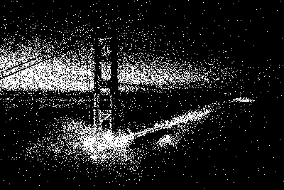
![К каждому пикселю перед квантованием добавлен случайный шум [-0.5; 0.5]](https://habrastorage.org/r/w1560/getpro/habr/upload_files/e3c/5c7/ebb/e3c5c7ebb28469d03e33342b53d75046.png "К каждому пикселю перед квантованием добавлен случайный шум [-0.5; 0.5]")
Этот результат показался мне довольно-таки неожиданным! Не назову его «хорошим», видеоигры из 90-х показали нам, что такие картинки могут выглядеть куда лучше. Но перед нами — быстрый способ, не требующий особых усилий, позволяющий получить больше деталей на монохромном изображении. И если бы я понимал слово «дизеринг» буквально, то на этом я и окончил бы статью. Но это — далеко не всё.
Дизеринг с упорядоченным шумом (ordered dithering)
Вместо того чтобы говорить о том, какой именно шум добавить к изображению перед квантованием, можно изменить точку зрения и обсудить настройку порога квантования.
// Добавление шума
grayscaleImage.mapSelf(brightness =>
  brightness + Math.random() - 0.5 > 0.5
    ? 1.0
    : 0.0
);

// Настройка порога квантования
grayscaleImage.mapSelf(brightness =>
  brightness > Math.random()
    ? 1.0
    : 0.0
);
В контексте монохромного дизеринга, где порог квантования равен 0.5, эти два подхода эквивалентны:
brightness+rand()-0.5 > 0.5
↔          brightness > 1.0-rand()
↔          brightness > rand()
Положительный момент этого подхода в том, что мы можем говорить о «матрице пороговых значений». Матрицы пороговых значений можно визуализировать. Это облегчит обсуждение того, почему результирующее изображение выглядит так, как выглядит. Ещё их можно вычислять заранее и использовать многократно, что делает процесс дизеринга детерминистическим и поддающимся параллелизации на уровне каждого пикселя. В результате дизеринг можно выполнять на GPU в виде шейдера. Именно так сделано в «Return of the Obra Dinn»! Есть несколько различных подходов к генерированию матриц пороговых значений, но все они каким-то образом упорядочивают шум, который добавляют к изображению. Отсюда и название этого метода — «дизеринг с упорядоченным шумом», или «дизеринг с упорядоченным возбуждением».
Матрица пороговых значений для вышеприведённого примера дизеринга — это, в буквальном смысле, матрица, полная случайных пороговых значений, называемых ещё «белым шумом» (white noise). Это название пришло из сферы обработки сигналов, где каждая частота имеет одинаковую интенсивность, как, например, в белом свете.

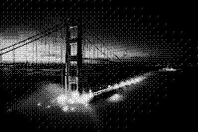
Дизеринг Байера (Bayer dithering)
Дизеринг Байера использует в роли матрицы пороговых значений матрицу Байера. Эти сущности названы в честь Брюса Байера, создателя фильтра Байера, который до наших дней используется в цифровых фотоаппаратах. Каждый пиксель светочувствительной матрицы может регистрировать лишь яркость света. Но если перед отдельными пикселями по-умному разместить цветные фильтры, можно восстановить цветное изображение посредством алгоритма демозаизации. Шаблон для этих фильтров — это тот же шаблон, что используется в дизеринге Байера.
Матрицы Байера бывают разных размеров, которые я, в итоге, стал называть «уровнями». Матрица Байера уровня 0 — это матрица 2×2. Уровень 1 — это матрица 4×4. А матрица уровня ![]() — это матрица
— это матрица ![]() . Матрицу уровня n можно рекурсивно вычислить из матрицы уровня
. Матрицу уровня n можно рекурсивно вычислить из матрицы уровня ![]() (хотя в Википедии, кроме того, упомянут алгоритм, основанный на работе с отдельными ячейками). Если ваше изображение оказалось больше, чем матрица Байера, можно обработать его, расположив несколько матриц пороговых значений рядом друг с другом.
(хотя в Википедии, кроме того, упомянут алгоритм, основанный на работе с отдельными ячейками). Если ваше изображение оказалось больше, чем матрица Байера, можно обработать его, расположив несколько матриц пороговых значений рядом друг с другом.

Матрица Байера уровня n содержит числа от 0 до ![]() После того, как вы нормализуете матрицу Байера, то есть — разделите на
После того, как вы нормализуете матрицу Байера, то есть — разделите на ![]() , её можно использовать как матрицу пороговых значений:
, её можно использовать как матрицу пороговых значений:
const bayer = generateBayerLevel(level);
grayscaleImage.mapSelf((brightness, { x, y }) =>
  brightness > bayer.valueAt(x, y, { wrap: true })
    ? 1.0
    : 0.0
);
Хочу отметить тут одну деталь: дизеринг Байера использующий матрицы, такие, которые определены выше, даст итоговое изображение, которые будет светлее исходного. Например — в области, где каждый пиксель имеет светлоту 1/255=0.4%, матрица Байера размера 2×2 сделает белым каждый из четырёх пикселей, что даст итоговую среднюю светлоту в 25%. Эта ошибка становится меньше при применении матриц Байера более высоких уровней, но фундаментальное отклонение от оригинала при этом остаётся таким же.

На нашем «тёмном» тестовом изображении небо не полностью чёрное, оно, при применении матрицы Байера уровня 0, оказывается значительно светлее. Хотя ситуация улучшается на более высоких уровнях, альтернативным решением может стать инвертирование отклонения, что приводит к получению изображений, которые темнее оригинала. Это делается путём обращения механизма использования матрицы Байера:
const bayer = generateBayerLevel(level);
grayscaleImage.mapSelf((brightness, { x, y }) =>
  //Обратите внимание на “1 -” в следующей строке
  brightness > 1 - bayer.valueAt(x, y, { wrap: true })
    ? 1.0
    : 0.0
);
Я использовал исходное определение матрицы Байера для «светлого» изображения и инвертированную версию для «тёмного» изображения. Лично мне больше всего нравятся результаты, полученные на уровнях 1 и 3.


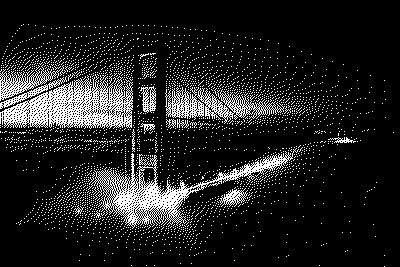
Дизеринг с синим шумом (blue noise)
И у подхода к дизерингу, когда применяется белый шум, и у того, где используется матрица Байера, конечно, есть недостатки. Для дизеринга Байера, например, характерно наложение на изображение повторяющихся структур, которые, особенно, если увеличить изображение, оказываются заметными. Белый шум — это набор случайных значений, что неизбежно ведёт к появлению на матрице пороговых значений «кластеров» из светлых пикселей и «пустот» из тёмных пикселей. Эти факты можно сделать более очевидными, если наклонить, или, если это для вас слишком сложно, алгоритмически размыть матрицу пороговых значений. «Кластеры» и «пустоты» могут плохо подействовать на результаты дизеринга. Если тёмные области изображения придутся на один из «кластеров» — в соответствующей области выходного изображения будут потеряны детали (и, наоборот, для светлых областей изображения, пришедшихся на «пустоты»).
")
Существует разновидность шума, называемая «синим шумом», нацеленная на решение этой проблемы. Этот шум называют «синим» из-за того, что сигналы более высоких частот в нём имеют более высокие интенсивности, чем сигналы более низких частот (как в случае с синим светом). Убирая или заглушая низкие частоты, можно сделать так, что «кластеры» и «пустоты» оказываются менее выраженными. Дизеринг с синим шумом выполняется так же быстро, как и дизеринг с белым шумом — в итоге это просто матрица пороговых значений, но генерирование синего шума немного сложнее и ресурсозатратнее.
Наиболее распространённый алгоритм генерирования синего шума, похоже, это «метод пустот и кластеров» («void-and-cluster method») Роберта Улични. Вот публикация, где это описано. По-моему, описание алгоритма не отличается интуитивной понятностью, а теперь, когда я его реализовал, я убедился в том, что он описан в чрезмерно абстрактном стиле. Но алгоритм это весьма толковый!
Алгоритм основан на идее, в соответствии с которой можно найти пиксель, являющийся частью «кластера» или «пустоты», обработав изображение с помощью эффекта размытия по Гауссу и найдя самый светлый (или, соответственно, самый тёмный) пиксель на размытом изображении. После инициализации чёрного изображения с помощью нескольких случайно расположенных белых пикселей, алгоритм приступает к непрерывной замене пикселей «кластеров» и «пустот», стремясь как можно равномернее распределить по изображению белые пиксели. После этого каждому пикселю назначается номер между 0 и ![]() (где
(где ![]() — общее количество пикселей) в соответствии с их важностью для формирования «кластеров» и «пустот». Подробности об этом смотрите здесь.
— общее количество пикселей) в соответствии с их важностью для формирования «кластеров» и «пустот». Подробности об этом смотрите здесь.
Моя реализация этого алгоритма работает хорошо, но не очень быстро, так как я не тратил много времени на её оптимизацию. На моём MacBook 2018 года генерирование текстуры синего шума размером 64×64 занимает около минуты. Для наших целей этого достаточно. Если нужно что-то побыстрее — стоит обратить внимание на оптимизацию, касающуюся эффекта размытия по Гауссу, но не в пространственной области, а в частотной области.
Отступление: конечно, я, когда это узнал, увидел интересную задачу, которую просто не мог не решить. Перспективность этой оптимизации объясняется свёрткой (это — внутренний механизм размытия по Гауссу), которой приходится проходиться по каждому полю ядра размытия по Гауссу для каждого пикселя изображения. Но если перевести и изображение, и ядро размытия по Гауссу в частотную область (используя один из многих алгоритмов быстрого преобразования Фурье), свёртка превращается в поэлементное умножение. Так как размер целевой текстуры синего шума — это степень двойки — я мог реализовать хорошо исследованный in-place-вариант алгоритма быстрого преобразования Фурье Кули — Тьюки. После нескольких первоначальных неудач я смог уменьшить время генерирования текстуры синего шума на 50%. Код у меня получился довольно-таки посредственный, поэтому тут найдётся место и для дальнейших оптимизаций.
. Чётких структур на размытом варианте изображения не осталось")
Синий шум основан на размытии по Гауссу, которое вычисляется на тороидальной структуре (это — замысловатый способ сказать, что алгоритм на краях изображения «сворачивается»). В результате изображение можно бесшовно «замостить» текстурами синего шума. Поэтому можно воспользоваться текстурой размера 64×64 и покрыть её копиями всё изображение. Дизеринг с синим шумом даёт приятную, сбалансированную отрисовку деталей, не выдавая заметных повторяющихся паттернов. Итоговое изображение смотрится органично.


Дизеринг с рассеянием ошибки (error diffusion)
Все вышеописанные подходы к дизерингу основаны на том факте, что ошибки квантования статистически сглаживаются из-за того, что пороговые значения в соответствующей матрице распределены равномерно. Но есть и другой подход к квантованию, связанный с рассеянием ошибки. Вы, скорее всего, встречались с ним, если когда-нибудь интересовались дизерингом. Применяя этот подход, мы не просто выполняем квантование изображения, надеясь, что, в среднем, ошибка квантования останется незначительной. Вместо этого мы измеряем ошибку квантования и рассеиваем эту ошибку на соседние пиксели, влияя на то, как они будут квантоваться. Мы, по сути, в процессе работы меняем изображение, которое хотим подвергнуть дизерингу. Это делает процесс преобразования изображения, по сути, последовательным.
Предостережение: одним из больших плюсов алгоритмов рассеяния ошибки, о котором мы не говорим в этом материале, является тот факт, что эти алгоритмы способны работать с произвольными цветовыми палитрами. А дизеринг с упорядоченным шумом требует, чтобы цвета на цветовой палитре были бы расположены с равными интервалами. Подробнее об этом я расскажу как-нибудь в другой раз.
Почти все подходы к дизерингу с рассеиванием ошибки, которые я собираюсь рассмотреть, используют «матрицу рассеяния», которая определяет то, как ошибка квантования текущего пикселя распространяется по соседним пикселям. При работе с такими матрицами часто считается, что пиксели изображения просматриваются сверху вниз и слева направо — так же, как читают тексты жители Запада. Это важно, так как ошибка может быть рассеяна лишь на пиксели, которые ещё не подверглись квантованию. Если вы будете обходить изображения в порядке, не соответствующем тому, на который рассчитана матрица рассеяния, соответствующим образом отразите матрицу.
Дизеринг с «простым» двумерным рассеянием ошибки
Примитивный подход к дизерингу с рассеянием ошибки предусматривает распространение ошибки квантования на пиксель, который находится ниже текущего, и на пиксель, находящийся справа от него. Это можно описать следующей матрицей:

Алгоритм рассеяния ошибки посещает каждый пиксель изображения (в правильном порядке), квантует текущий пиксель и измеряет ошибку квантования. Обратите внимание на то, что значение ошибки квантования имеет знак, то есть — оно может быть отрицательным, если квантование делает пиксель светлее, чем исходный пиксель. Затем части ошибки добавляют к соседним пикселям в соответствии с матрицей. Потом этот процесс повторяется для следующего пикселя.
Пошаговая визуализация алгоритма рассеяния ошибки
Эта анимация предназначена для визуализации алгоритма, но она не способна показать то, как результаты дизеринга соотносятся с оригиналом изображения. Области размером 4×4 пикселя вряд ли достаточно для того, чтобы рассеять и усреднить ошибки квантования. Но тут можно видеть то, что если пиксель в ходе квантования делается светлее, то соседние пиксели, чтобы это скомпенсировать, делаются темнее (и наоборот).


Но простота матрицы рассеяния делает рассматриваемый подход к дизерингу подверженным появлению различимых паттернов, вроде паттернов в виде линий, которые можно видеть на вышеприведённых изображениях.
Дизеринг по алгоритму Флойда — Стейнберга (Floyd-Steinberg)
Алгоритм Флойда — Стейнберга — это, пожалуй, один из самых известных алгоритмов рассеяния ошибки, а, возможно, это — самый известный алгоритм, применяемый при дизеринге изображений. Он использует более сложную матрицу рассеяния ошибок, которая позволяет распределять ошибку на все непосещённые пиксели, являющиеся непосредственными соседями текущего пикселя. Числа в этой матрице тщательно подобраны для того чтобы как можно сильнее уменьшить возможность образования повторяющихся паттернов.

Применение алгоритма Флойда — Стейнберга — это большой шаг вперёд в нашем исследовании, так как это позволяет предотвращать возникновение множества паттернов. Но и при его применении большие пространства изображения с незначительным количеством деталей всё ещё могут выглядеть не очень хорошо.

Дизеринг по алгоритму Джарвиса — Джудиса — Нинке (Jarvis-Judice-Ninke)
В алгоритме Джарвиса — Джудиса — Нинке используется ещё большая матрица рассеяния ошибки. Ошибка распределяется на большее количество пикселей, а не только на те, которые находятся в непосредственной близости от текущего пикселя.

Использование такой матрицы рассеяния ошибки ведёт к дальнейшему снижению вероятности образования паттернов. И хотя на тестовых изображениях имеются паттерны в виде линий, теперь они не так сильно бросаются в глаза.


Дизеринг по алгоритму Аткинсона (Atkinson)
Алгоритм Аткинсона был разработан в компании Apple Биллом Аткинсоном и получил известность благодаря его использованию в ранних компьютерах Macintosh.

Стоит отметить, что матрица рассеяния ошибки Аткинсона состоит из шести единиц, но она нормализуется с использованием 1/8, то есть — она не переносит всю ошибку на соседние пиксели, увеличивая воспринимаемую контрастность изображения.


Дизеринг по алгоритму Римерсма (Riemersma)
Честно говоря, на алгоритм Римерсма я наткнулся случайно. Я, пока исследовал другие алгоритмы, нашёл одну обстоятельную статью, в которой было написано об этом алгоритме. Такое ощущение, что он не особенно широко известен, но он мне очень понравился. Понравились мне и те идеи, на которых он основан. Вместо того, чтобы, ряд за рядом, обходить изображение, он обходит изображение по кривой Гильберта. С технической точки зрения тут подошла бы любая кривая, заполняющая пространство. Но рекомендуется использовать именно кривую Гильберта. Этот алгоритм довольно просто реализовать с использованием генераторов. Благодаря этому алгоритм нацелен на то, чтобы взять лучшее из алгоритмов дизеринга с упорядоченным шумом и с рассеянием ошибки. Речь идёт об ограничении количества пикселей, на которые может подействовать один пиксель, а так же о приятном внешнем виде результата (и о скромных требованиях к памяти).

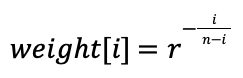
У кривой Гильберта есть свойство «локальности», которое выражается в том, что пиксели, находящиеся близко друг к другу на кривой, находятся близко друг к другу и на изображении. При таком подходе нам не нужно использовать матрицу рассеяния ошибки. Вместо этого достаточно применить последовательность рассеяния ошибки длиной n. Для квантования текущего пикселя к нему добавляются n последних ошибок квантования с весами, заданными в последовательности рассеяния ошибки. В вышеупомянутой статье для задания весов используется экспоненциальный спад. Ошибке квантования предыдущего пикселя назначается вес 1, самой старой ошибке квантования в списке назначается маленький, вычисляемый по особой формуле, вес ![]() . Для вычисления
. Для вычисления ![]() -го веса используется следующая формула:
-го веса используется следующая формула:
В статье рекомендуется использовать ![]() , а минимальный размер списка значений —
, а минимальный размер списка значений — ![]() , но, выполняя тесты, я обнаружил, что лучше всего выглядит изображение с
, но, выполняя тесты, я обнаружил, что лучше всего выглядит изображение с ![]() и
и ![]()


Результат выглядит чрезвычайно органично, почти так же приятно, как после дизеринга с синим шумом. И, в то же время, дизеринг по алгоритму Римерсма легче реализовать, чем оба предыдущих варианта. Это, правда, всё равно, алгоритм, основанный на рассеянии ошибки, то есть — он обрабатывает данные последовательно и не подходит для выполнения на GPU.
Я выбираю синий шум, дизеринг Байера и алгоритм Римерсма
«Return of the Obra Dinn» — это 3D-игра, поэтому в ней необходимо использовать дизеринг с упорядоченным шумом для того чтобы выполнять соответствующий код в виде шейдера. В ней используется и дизеринг Байера, и дизеринг с синим шумом. Я поддерживаю создателей игры в этом выборе и тоже считаю, что, с эстетической точки зрения, они дают наиболее приятные результаты. Дизеринг Байера даёт немного больше структуры, а изображения после дизеринга с синим шумом выглядят очень естественно и органично. Я, кроме того, хочу особо выделить дизеринг по алгоритму Римерсма, и мне хочется узнать о том, как он показывает себя на изображениях с многоцветной палитрой.
Большая часть окружения в «Obra Dinn» рендерится с применением дизеринга с синим шумом. Люди и другие интересные объекты обрабатываются с помощью дизеринга Байера. Это создаёт интересный визуальный контраст и выделяет их, не нарушая общую эстетику игры. Напомню, что подробности о том, почему в игре всё сделано именно так, и о том, как обрабатываются перемещения камеры, можно почитать в посте Лукаса Поупа.
Если вы хотите испытать разные алгоритмы дизеринга на своём изображении — взгляните на мою демо-страницу, использованную для создания всех примеров к этой статье. Учитывайте, что мои реализации алгоритмов дизеринга не относятся к разряду самых быстрых. Поэтому, если вы решите «скормить» моей программе 20-мегапиксельную JPEG-фотографию — её обработка займёт некоторое время.
Обратите внимание на то, что у меня такое ощущение, что в Safari я наткнулся на деоптимизацию. Так, в Chrome на работу моего генератора синего шума требуется примерно 30 секунд, а в Safari — более 20 минут. А вот в Safari Tech Preview генератор работает гораздо быстрее.
Уверен, что то, о чём я рассказал — это до крайности нишевая тема, но мне понравилось побывать в этой кроличьей норе. Если вам есть что сказать о дизеринге, если вы этим занимались — с радостью вас послушаю.
Благодарности и дополнительные материалы
Благодарю Лукаса Поупа за его игры и за источник визуального вдохновения.
Благодарю Кристофа Питерса за его замечательную статью о генерировании синего шума.
О, а приходите к нам работать? 🤗 💰
Мы в wunderfund.io занимаемся высокочастотной алготорговлей с 2014 года. Высокочастотная торговля — это непрерывное соревнование лучших программистов и математиков всего мира. Присоединившись к нам, вы станете частью этой увлекательной схватки.
Мы предлагаем интересные и сложные задачи по анализу данных и low latency разработке для увлеченных исследователей и программистов. Гибкий график и никакой бюрократии, решения быстро принимаются и воплощаются в жизнь.
Сейчас мы ищем плюсовиков, питонистов, дата-инженеров и мл-рисерчеров.
Присоединяйтесь к нашей команде.
помогите разобрать в настройках версы
-
spartaks2007
- Постоянный участник

- Сообщения: 175
- Зарегистрирован: 30 июл 2013 23:33
- Последний визит: 23 янв 2023 12:14
- Изменить репутацию:
Репутация: нет - Откуда: Брянск

помогите разобрать в настройках версы
Добрый день., прошу не пинать, что означает и как проявляется на печати настройки в печати Версаворкс :
1)Полутона- выбор Dither и Erorr Difusion(V)
2)Интерполяция -Neareset N. — b-liner- Be Cubic
3) Направление be-deriction — Uni deriction
Может есть мануал с описанием, буду при много благодарен!
-
mks.mpei
- Старожил
- Сообщения: 1102
- Зарегистрирован: 21 май 2016 18:12
- Последний визит: 09 фев 2023 11:10
- Изменить репутацию:
Репутация:
Голосов: 15 - Откуда: Москва

Re: помогите разобрать в настройках версы
Сообщение mks.mpei » 01 ноя 2022 19:44
spartaks2007 есть гугл и яндекс)
Error diffusion качественнее, но риповка в 2 раза дольше.
Unidir качественнее bidir, но имеет смысл только на самых мелких элементах или при проблемах с печатью
Вернуться в «Прочие программные пакеты…»
Кто сейчас на конференции
Сейчас этот форум просматривают: нет зарегистрированных пользователей и 0 гостей

This paper introduces a patent-free¹ positional (ordered) dithering algorithm
that is applicable for arbitrary palettes. Such dithering algorithm
can be used to change truecolor animations into paletted ones, while
maximally avoiding unintended jitter arising from dithering.

For most of the article, we will use this example truecolor picture
and palette.
The scene is from a PSX game called Chrono Cross, and the palette
has been manually selected for this particular task.
You may immediately notice that the palette is not regular; although there
are clearly some gradients, the gradients are not regularly spaced.
Undithered rendering

Undithered rendering is, in pseudo code:
  For each pixel, Input, in the original picture:
    Color = FindClosestColorFrom(Palette, Input)
    Draw pixel using that color.
It will produce a picture like that on the left.
The exact appearance depends on the particular «closest color» function.
Most software uses a simple euclidean RGB distance to determine
how well colors match, i.e.
√(ΔRed² + ΔGreen² + ΔBlue²)
.
We will also begin from there.
Error diffusion dithers

Error diffusion dithers work by distributing an error to neighboring
pixels in hope that one error won’t show when the whole picture
is equally off. Although it works great for static pictures, it won’t
work for animation.
On the right is an animation with the single static screenshot shown above.
A single yellow pixel was added to the image and moved around.
The animation has been quantized to 16 colors and dithered
using Floyd-Steinberg dithering. An entire cone of jittering
artifacts gets spawned from that single point downwards and to the right.
There exist different error diffusion dithers, but they all suffer from the
same problem. Aside from Riemersma (which walks through the pixels in
a non-linear order) and Scolorq (which treats an entire image at once),
they all use the same algorithm, only differing on the
diffusion map
that they use.
Standard ordered dithering algorithm
Standard ordered dithering, which uses the Bayer threshold matrix, is:
  Threshold = COLOR(256/4, 256/4, 256/4); /* Estimated precision of the palette */
  For each pixel, Input, in the original picture:
    Factor  = ThresholdMatrix[xcoordinate % X][ycoordinate % Y];
    Attempt = Input + Factor * Threshold
    Color = FindClosestColorFrom(Palette, Attempt)
    Draw pixel using Color
If we translate this into PHP, a whole test program becomes
(using the image and palette that is described after the program):
<?php

/* Create a 8x8 threshold map */
$map = array_map(function($p)
                 {
                   $q = $p ^ ($p >> 3);
                   return ((($p & 4) >> 2) | (($q & 4) >> 1)
                         | (($p & 2) << 1) | (($q & 2) << 2)
                         | (($p & 1) << 4) | (($q & 1) << 5)) / 64.0;
                 }, range(0,63));

/* Define palette */
$pal = Array(0x080000,0x201A0B,0x432817,0x492910,
             0x234309,0x5D4F1E,0x9C6B20,0xA9220F,
             0x2B347C,0x2B7409,0xD0CA40,0xE8A077,
             0x6A94AB,0xD5C4B3,0xFCE76E,0xFCFAE2);

/* Read input image */
$srcim = ImageCreateFromPng('scene.png');
$w = ImageSx($srcim);
$h = ImageSy($srcim);

/* Create paletted image */
$im = ImageCreate($w,$h);
foreach($pal as $c) ImageColorAllocate($im, $c>>16, ($c>>8)&0xFF, $c&0xFF);

$thresholds = Array(256/4, 256/4, 256/4);

/* Render the paletted image by converting each input pixel using the threshold map. */
for($y=0; $y<$h; ++$y)
  for($x=0; $x<$w; ++$x)
  {
    $map_value = $map[($x & 7) + (($y & 7) << 3)];
    $color = ImageColorsForIndex($srcim, ImageColorAt($srcim, $x,$y));
    $r = (int)($color['red']   + $map_value * $thresholds[0]);
    $g = (int)($color['green'] + $map_value * $thresholds[1]);
    $b = (int)($color['blue']  + $map_value * $thresholds[2]);
    /* Plot using the palette index with color that is closest to this value */
    ImageSetPixel($im, $x,$y, ImageColorClosest($im, $r,$g,$b));
  }
ImagePng($im, 'scenebayer0.png');
Here is what this program produces:


There are many immediate problems one may notice in this picture, the most
important being that it simply looks bad.
The reason why this is an inadequate algorithm as is is because the algorithm
assumes that the palette contains equally spaced elements on each of the R,G,B axis.
An example of such palette is the web-safe palette (shown on the right),
which contains colors for each combination of six-bit red, green and blue.
However, in practical applications, this is rarely the case. An example would
be developing a game for a handheld device that can only display 16 simultaneous
colors from a larger palette. The 16 colors would have to be an optimal
representation of the colors present in original graphics.
Although the algorithm can be slightly improved by measuring rather than
estimating the maximum distance between successive values on each channel
in the palette (below), such improvements only rarely give a
satisfying outcome. They also tend to reduce the dithering
benefits (compare the hanging gray curtain before and after).

/* Find the maximum distance between successive values on each channel in the palette */
$thresholds = Array(0, 0, 0);
foreach($thresholds as $channel => &$t)
{
  $values = array_map(function($val) use($channel)
                      {
                        return ($val >> ($channel*8)) & 0xFF;
                      }, $pal);
  sort($values); /* Sort the color values of the palette in ascending order */
  array_reduce($values,
               function($p,$val) use(&$t) { $t = max($t, $val-$p); return $val; },
               $values[0]);
}
We present here several algorithms that have the «goods» from
Bayer’s ordered dithering algorithm (namely, the color of a pixel
depends on that pixel alone, making it suitable for animations),
but is applicable to arbitrary palettes.
Yliluoma’s ordered dithering algorithm 1
We begin by making the observation that the ordered dithering algorithm
always mixes two colors together in a variable proportion.
Using the same principle, we begin by envisioning a method
of optimizing that pair of colors:
  For each pixel, Input, in the original picture:
    Factor  = ThresholdMatrix[xcoordinate % X][ycoordinate % Y];
    Make a Plan, based on Input and the Palette.

    If Factor < Plan.ratio,
      Draw pixel using Plan.color2
    else,
      Draw pixel using Plan.color1
The Planning procedure can be implemented as follows:
  SmallestPenalty = 10^99 /* Impossibly large number */
  For each unique combination of two colors from the palette, Color1 and Color2:
    For each possible Ratio, 0 .. (X*Y-1):
      /* Determine what mixing the two colors in this proportion will produce */
      Mixed = Color1 + Ratio * (Color2 - Color1) / (X*Y)
      /* Rate how well it matches what we want to accomplish */
      Penalty = Evaluate the difference of Input and Mixed.
      /* Keep the result that has the smallest error */
      If Penalty < SmallestPenalty,
        SmallestPenalty = Penalty
        Plan = { Color1, Color2, Ratio / (X*Y) }.
This function runs for
M × N × (N −1) ÷ 2 + N
iterations for a palette of size N and a dithering pattern of size M = X×Y,
complexity being O(N²×M), and it depends on an evaluation function.
The evaluation function might be defined using an euclidean distance
between the two colors, considered as three-dimensional vectors
formed by the Red, Green and Blue color components, i.e.
√(ΔRed² + ΔGreen² + ΔBlue²) as discussed earlier.
The whole program becomes in C++:
#include <gd.h>
#include <stdio.h>

/* 8x8 threshold map */
#define d(x) x/64.0
static const double map[8*8] = {
d( 0), d(48), d(12), d(60), d( 3), d(51), d(15), d(63),
d(32), d(16), d(44), d(28), d(35), d(19), d(47), d(31),
d( 8), d(56), d( 4), d(52), d(11), d(59), d( 7), d(55),
d(40), d(24), d(36), d(20), d(43), d(27), d(39), d(23),
d( 2), d(50), d(14), d(62), d( 1), d(49), d(13), d(61),
d(34), d(18), d(46), d(30), d(33), d(17), d(45), d(29),
d(10), d(58), d( 6), d(54), d( 9), d(57), d( 5), d(53),
d(42), d(26), d(38), d(22), d(41), d(25), d(37), d(21) };
#undef d

/* Palette */
static const unsigned pal[16] =
{0x080000,0x201A0B,0x432817,0x492910,
 0x234309,0x5D4F1E,0x9C6B20,0xA9220F,
 0x2B347C,0x2B7409,0xD0CA40,0xE8A077,
 0x6A94AB,0xD5C4B3,0xFCE76E,0xFCFAE2 };

// Compare the difference of two RGB values
double ColorCompare(int r1,int g1,int b1, int r2,int g2,int b2)
{
    double diffR = (r1-r2)/255.0, diffG = (g1-g2)/255.0, diffB = (b1-b2)/255.0;
    return diffR*diffR + diffG*diffG + diffB*diffB;
}
double EvaluateMixingError(int r,int g,int b,    // Desired color
                           int r0,int g0,int b0, // Mathematical mix product
                           int r1,int g1,int b1, // Mix component 1
                           int r2,int g2,int b2, // Mix component 2
                           double ratio)         // Mixing ratio
{
    return ColorCompare(r,g,b, r0,g0,b0);
}

struct MixingPlan
{
    unsigned colors[2];
    double ratio; /* 0 = always index1, 1 = always index2, 0.5 = 50% of both */
};
MixingPlan DeviseBestMixingPlan(unsigned color)
{
    const unsigned r = color>>16, g = (color>>8)&0xFF, b = color&0xFF;
    MixingPlan result = { {0,0}, 0.5 };
    double least_penalty = 1e99;
    // Loop through every unique combination of two colors from the palette,
    // and through each possible way to mix those two colors. They can be
    // mixed in exactly 64 ways, when the threshold matrix is 8x8.
    for(unsigned index1 = 0;      index1 < 16; ++index1)
    for(unsigned index2 = index1; index2 < 16; ++index2)
    for(unsigned ratio=0; ratio<64; ++ratio)
    {
        if(index1 == index2 && ratio != 0) break;
        // Determine the two component colors
        unsigned color1 = pal[index1], color2 = pal[index2];
        unsigned r1 = color1>>16, g1 = (color1>>8)&0xFF, b1 = color1&0xFF;
        unsigned r2 = color2>>16, g2 = (color2>>8)&0xFF, b2 = color2&0xFF;
        // Determine what mixing them in this proportion will produce
        unsigned r0 = r1 + ratio * int(r2-r1) / 64;
        unsigned g0 = g1 + ratio * int(g2-g1) / 64;
        unsigned b0 = b1 + ratio * int(b2-b1) / 64;
        // Determine how well that matches what we want to accomplish
        double penalty = EvaluateMixingError(r,g,b, r0,g0,b0, r1,g1,b1, r2,g2,b2, ratio/64.0);
        if(penalty < least_penalty)
        {
            // Keep the result that has the smallest error
            least_penalty = penalty;
            result.colors[0] = index1;
            result.colors[1] = index2;
            result.ratio = ratio / 64.0;
        }
    }
    return result;
}

int main()
{
    FILE* fp = fopen("scene.png", "rb");
    gdImagePtr srcim = gdImageCreateFromPng(fp);
    fclose(fp);

    unsigned w = gdImageSX(srcim), h = gdImageSY(srcim);
    gdImagePtr im = gdImageCreate(w, h);
    for(unsigned c=0; c<16; ++c)
        gdImageColorAllocate(im, pal[c]>>16, (pal[c]>>8)&0xFF, pal[c]&0xFF);
  #pragma omp parallel for
    for(unsigned y=0; y<h; ++y)
        for(unsigned x=0; x<w; ++x)
        {
          double map_value = map[(x & 7) + ((y & 7) << 3)];
          unsigned color = gdImageGetTrueColorPixel(srcim, x, y);
          MixingPlan plan = DeviseBestMixingPlan(color);
          gdImageSetPixel(im, x,y, plan.colors[ map_value < plan.ratio ? 1 : 0 ] );
        }
    fp = fopen("scenedither1.png", "wb");
    gdImagePng(im, fp);
    fclose(fp); gdImageDestroy(im); gdImageDestroy(srcim);
}
The result of this program is shown below (on the right-hand side, the standard ordered-dithered version):

There are two problems with this trivial implementation:
- It is very slow.
- There is a lot of visual noise.
On the other hand, there are two advantages visible already:
- Overall, there is a lot more color [than in the standard version], and the scene does not look that washed out anymore.
This is the mathematically correct result, assuming gamma of 1.0.
If one substitutes temporal dithering for the spatial dithering,
it is easy to see that the wild dithering patterns do indeed produce,
by average, colors very close to the originals. However, the human brain
just sees a lot of bright and dim pixels where there should be none.
Temporal dithering will be covered later in this article.
Therefore, psychovisual concerns must also be accounted for when
implementing this algorithm.
Consider this example palette: #000000, #FFFFFFF, #7E8582, #8A7A76.
For producing a color #808080, one might combine the two extremes,
black and white. However, this produces a very nasty visual effect.
It is better to combine the two slightly tinted values near the
intended result, even though it produces #847F7C, a noticeably
red-tinted gray value, rather than the mathematically
accurate #808080 that would be acquired from combining the two other values.
The psychovisual model that we introduce, consists of three parts:
- Algorithm for comparing the similarity of two color values.
- Criteria for deciding which pixels can be paired together.
- Gamma correction (technically not psychovisual, because it is just physics).
Psychovisual model
The simplest way to adjust the psychovisual model is to add some code
that considers the difference between the two pixel values that are being
mixed in the dithering process, and penalizes combinations that differ
too much.
double EvaluateMixingError(int r,int g,int b,    // Desired color
                           int r0,int g0,int b0, // Mathematical mix product
                           int r1,int g1,int b1, // Mix component 1
                           int r2,int g2,int b2, // Mix component 2
                           double ratio)         // Mixing ratio
{
    return ColorCompare(r,g,b, r0,g0,b0)
         + ColorCompare(r1,g1,b1, r2,g2,b2)*0.1;
}
The result is shown below:

Though the result looks very nice now, there are still many ways the
algorithm can still be improved. For instance, the color comparison
function could be improved by a great deal.
Wikipedia has an entire article
about the topic of comparing two color values.
Most of the improved color comparison functions are based on the CIE
colorspace, but simple improvements can be done in the RGB space too.
Such a simple improvement is shown below. We might call this RGBL,
for luminance-weighted RGB.
The EvaluateMixingError function was also changed to weigh the
component difference only in inverse proportion to the mixing evenness.
// Compare the difference of two RGB values, weigh by CCIR 601 luminosity:
double ColorCompare(int r1,int g1,int b1, int r2,int g2,int b2)
{
    double luma1 = (r1*299 + g1*587 + b1*114) / (255.0*1000);
    double luma2 = (r2*299 + g2*587 + b2*114) / (255.0*1000);
    double lumadiff = luma1-luma2;
    double diffR = (r1-r2)/255.0, diffG = (g1-g2)/255.0, diffB = (b1-b2)/255.0;
    return (diffR*diffR*0.299 + diffG*diffG*0.587 + diffB*diffB*0.114)*0.75
         + lumadiff*lumadiff;
}

double EvaluateMixingError(int r,int g,int b,
                           int r0,int g0,int b0,
                           int r1,int g1,int b1,
                           int r2,int g2,int b2,
                           double ratio)
{
    return ColorCompare(r,g,b, r0,g0,b0)
         + ColorCompare(r1,g1,b1, r2,g2,b2) * 0.1 * (fabs(ratio-0.5)+0.5);
}
The result is shown below. Improvements can be seen in the rightside
window and in the girl’s skirt, among other places.

Left: After tweaking the color comparison function.
Right: Before tweaking the color comparison function.
Refinements
This version of DeviseBestMixingPlan calculates the mixing ratio mathematically
rather than by iterating. It ends up being about 64 times faster than the
iterating version, and differs only neglibly.
The function now runs for N²÷2 iterations for a palette of size N.
MixingPlan DeviseBestMixingPlan(unsigned color)
{
    const unsigned r = color>>16, g = (color>>8)&0xFF, b = color&0xFF;
    MixingPlan result = { {0,0}, 0.5 };
    double least_penalty = 1e99;
    for(unsigned index1 = 0; index1 < 16; ++index1)
    for(unsigned index2 = index1; index2 < 16; ++index2)
    {
        // Determine the two component colors
        unsigned color1 = pal[index1], color2 = pal[index2];
        unsigned r1 = color1>>16, g1 = (color1>>8)&0xFF, b1 = color1&0xFF;
        unsigned r2 = color2>>16, g2 = (color2>>8)&0xFF, b2 = color2&0xFF;
        int ratio = 32;
        if(color1 != color2)
        {
            // Determine the ratio of mixing for each channel.
            //   solve(r1 + ratio*(r2-r1)/64 = r, ratio)
            // Take a weighed average of these three ratios according to the
            // perceived luminosity of each channel (according to CCIR 601).
            ratio = ((r2 != r1 ? 299*64 * int(r - r1) / int(r2-r1) : 0)
                  +  (g2 != g1 ? 587*64 * int(g - g1) / int(g2-g1) : 0)
                  +  (b1 != b2 ? 114*64 * int(b - b1) / int(b2-b1) : 0))
                  / ((r2 != r1 ? 299 : 0)
                   + (g2 != g1 ? 587 : 0)
                   + (b2 != b1 ? 114 : 0));
            if(ratio < 0) ratio = 0; else if(ratio > 63) ratio = 63;
        }
        // Determine what mixing them in this proportion will produce
        unsigned r0 = r1 + ratio * int(r2-r1) / 64;
        unsigned g0 = g1 + ratio * int(g2-g1) / 64;
        unsigned b0 = b1 + ratio * int(b2-b1) / 64;
        double penalty = EvaluateMixingError(
            r,g,b, r0,g0,b0, r1,g1,b1, r2,g2,b2,
            ratio / double(64));
        if(penalty < least_penalty)
        {
            least_penalty = penalty;
            result.colors[0] = index1;
            result.colors[1] = index2;
            result.ratio = ratio / double(64);
        }
    }
    return result;
}
With these changes, the rendering result becomes:

Left: Faster planner
Right: Slower and more thorough planner
The quality did suffer slightly, but the faster rendering might still be worth it.
When non-realtime rendering is not desired, such as when pre-rendering
static pictures or animations for later presentation,
one might want to strive for better quality and continue using the slower,
looping method.
The remainder of this article’s pictures will continue using the loop.
Tri-tone dithering

The final improvement for this algorithm for now
that is covered in this article is tri-tone dithering.
It is a three-color dithering algorithm with a fixed 2×2 matrix, where one of
the colors occurs at 50% proportion and the others occur at 25% proportion.
An example of using this approach is shown on the right.
The complete source code is shown below.
The DeviseBestMixingPlan function now runs for
N² × (N − 1) ÷ 2
iterations for a palette of size N, for
a complexity of O(N3).
#include <gd.h>
#include <stdio.h>
#include <math.h>

/* 8x8 threshold map */
#define d(x) x/64.0
static const double map[8*8] = {
d( 0), d(48), d(12), d(60), d( 3), d(51), d(15), d(63),
d(32), d(16), d(44), d(28), d(35), d(19), d(47), d(31),
d( 8), d(56), d( 4), d(52), d(11), d(59), d( 7), d(55),
d(40), d(24), d(36), d(20), d(43), d(27), d(39), d(23),
d( 2), d(50), d(14), d(62), d( 1), d(49), d(13), d(61),
d(34), d(18), d(46), d(30), d(33), d(17), d(45), d(29),
d(10), d(58), d( 6), d(54), d( 9), d(57), d( 5), d(53),
d(42), d(26), d(38), d(22), d(41), d(25), d(37), d(21) };
#undef d

/* Palette */
static const unsigned pal[16] =
{0x080000,0x201A0B,0x432817,0x492910,
 0x234309,0x5D4F1E,0x9C6B20,0xA9220F,
 0x2B347C,0x2B7409,0xD0CA40,0xE8A077,
 0x6A94AB,0xD5C4B3,0xFCE76E,0xFCFAE2 };

double ColorCompare(int r1,int g1,int b1, int r2,int g2,int b2)
{
    double luma1 = (r1*299 + g1*587 + b1*114) / (255.0*1000);
    double luma2 = (r2*299 + g2*587 + b2*114) / (255.0*1000);
    double lumadiff = luma1-luma2;
    double diffR = (r1-r2)/255.0, diffG = (g1-g2)/255.0, diffB = (b1-b2)/255.0;
    return (diffR*diffR*0.299 + diffG*diffG*0.587 + diffB*diffB*0.114)*0.75
         + lumadiff*lumadiff;
}
double EvaluateMixingError(int r,int g,int b,
                           int r0,int g0,int b0,
                           int r1,int g1,int b1,
                           int r2,int g2,int b2,
                           double ratio)
{
    return ColorCompare(r,g,b, r0,g0,b0)
         + ColorCompare(r1,g1,b1, r2,g2,b2)*0.1*(fabs(ratio-0.5)+0.5);
}

struct MixingPlan
{
    unsigned colors[4];
    double ratio;
    /* 0 = always index1, 1 = always index2, 0.5 = 50% of both */
    /* 4 = special three or four-color dither */
};
MixingPlan DeviseBestMixingPlan(unsigned color)
{
    const unsigned r = color>>16, g = (color>>8)&0xFF, b = color&0xFF;
    MixingPlan result = { {0,0}, 0.5 };
    double least_penalty = 1e99;
    for(unsigned index1 = 0; index1 < 16; ++index1)
    for(unsigned index2 = index1; index2 < 16; ++index2)
    //for(int ratio=0; ratio<64; ++ratio)
    {
        // Determine the two component colors
        unsigned color1 = pal[index1], color2 = pal[index2];
        unsigned r1 = color1>>16, g1 = (color1>>8)&0xFF, b1 = color1&0xFF;
        unsigned r2 = color2>>16, g2 = (color2>>8)&0xFF, b2 = color2&0xFF;
        int ratio = 32;
        if(color1 != color2)
        {
            // Determine the ratio of mixing for each channel.
            //   solve(r1 + ratio*(r2-r1)/64 = r, ratio)
            // Take a weighed average of these three ratios according to the
            // perceived luminosity of each channel (according to CCIR 601).
            ratio = ((r2 != r1 ? 299*64 * int(r - r1) / int(r2 - r1) : 0)
                  +  (g2 != g1 ? 587*64 * int(g - g1) / int(g2 - g1) : 0)
                  +  (b1 != b2 ? 114*64 * int(b - b1) / int(b2 - b1) : 0))
                  / ((r2 != r1 ? 299 : 0)
                   + (g2 != g1 ? 587 : 0)
                   + (b2 != b1 ? 114 : 0));
            if(ratio < 0) ratio = 0; else if(ratio > 63) ratio = 63;
        }
        // Determine what mixing them in this proportion will produce
        unsigned r0 = r1 + ratio * int(r2-r1) / 64;
        unsigned g0 = g1 + ratio * int(g2-g1) / 64;
        unsigned b0 = b1 + ratio * int(b2-b1) / 64;
        double penalty = EvaluateMixingError(
            r,g,b, r0,g0,b0, r1,g1,b1, r2,g2,b2,
            ratio / double(64));
        if(penalty < least_penalty)
        {
            least_penalty = penalty;
            result.colors[0] = index1;
            result.colors[1] = index2;
            result.ratio = ratio / double(64);
        }
        if(index1 != index2)
        for(unsigned index3 = 0; index3 < 16; ++index3)
        {
            if(index3 == index2 || index3 == index1) continue;
            // 50% index3, 25% index2, 25% index1
            unsigned color3 = pal[index3];
            unsigned r3 = color3>>16, g3 = (color3>>8)&0xFF, b3 = color3&0xFF;
            r0 = (r1 + r2 + r3*2) / 4;
            g0 = (g1 + g2 + g3*2) / 4;
            b0 = (b1 + b2 + b3*2) / 4;
            penalty = ColorCompare(r,g,b, r0,g0,b0)
                    + ColorCompare(r1,g1,b1, r2,g2,b2)*0.025
                    + ColorCompare((r1+g1)/2,(g1+g2)/2,(b1+b2)/2, r3,g3,b3)*0.025;
            if(penalty < least_penalty)
            {
                least_penalty = penalty;
                result.colors[0] = index3; // (0,0) index3 occurs twice
                result.colors[1] = index1; // (0,1)
                result.colors[2] = index2; // (1,0)
                result.colors[3] = index3; // (1,1)
                result.ratio = 4.0;
            }
        }
    }
    return result;
}

int main(int argc, char**argv)
{
    FILE* fp = fopen(argv[1], "rb");
    gdImagePtr srcim = gdImageCreateFromPng(fp);
    fclose(fp);

    unsigned w = gdImageSX(srcim), h = gdImageSY(srcim);
    gdImagePtr im = gdImageCreate(w, h);
    for(unsigned c=0; c<16; ++c)
        gdImageColorAllocate(im, pal[c]>>16, (pal[c]>>8)&0xFF, pal[c]&0xFF);
  #pragma omp parallel for
    for(unsigned y=0; y<h; ++y)
        for(unsigned x=0; x<w; ++x)
        {
            unsigned color = gdImageGetTrueColorPixel(srcim, x, y);
            MixingPlan plan = DeviseBestMixingPlan(color);
            if(plan.ratio == 4.0) // Tri-tone or quad-tone dithering
            {
                gdImageSetPixel(im, x,y, plan.colors[ ((y&1)*2 + (x&1)) ]);
            }
            else
            {
                double map_value = map[(x & 7) + ((y & 7) << 3)];
                gdImageSetPixel(im, x,y, plan.colors[ map_value < plan.ratio ? 1 : 0 ]);
            }
        }
    fp = fopen(argv[2], "wb");
    gdImagePng(im, fp);
    fclose(fp); gdImageDestroy(im); gdImageDestroy(srcim);
}
It is also possible to implement quad-tone dithering,
but it is too slow to calculate (O(N^4) runtime) using
this algorithm. We’ll return to that topic later.
Yliluoma’s ordered dithering algorithm 2
An altogetherly different dithering algorithm can be devised by discarding
the initial assumption that the dithering mixes two colortones together,
and instead, assuming that each matrix value corresponds to a particular
color tone. A 8×8 matrix has 64 color tones, a 2×2 matrix has 4 color tones,
and so on.
An algorithm for populating such a color array will need to find the N-term
expression of color values that, when combined, will produce the closest
approximation of the input color.
One such algorithm is to start with a guess (the closest color), and then
find out how much it went wrong, and then find out by experimentation which
terms are needed to improve the result.
To solve the issue about pixel orientations changing, the colors will
be sorted by luma. They will still change relative orientation, but
such action is relatively minor.
In pseudo code, the process of converting
the input bitmap into a target bitmap goes like this:
  For each pixel, Input, in the original picture:
    Achieved      = 0      // Total color sum achieved so far
    CandidateList.clear()
    LoopWhile CandidateList.Size < (X * Y)
      Count     = 1
      Candidate = 0 // Candidate color from palette
      Comparison.reset()
      Max = CandidateList.Size, Or 1 if empty
      For each Color in palette:
        AddingCount = 1
        LoopWhile AddingCount <= Max
          Sum         = Achieved + Color * AddingCount
          Divide      = CandidateList.Size + AddingCount
          Test        = Sum / Divide
          Compare Test to Input using CIEDE2000 or RGB;
          If it was the best match since Comparison was reset:
            Candidate := Color
            Count     := AddingCount
          EndCompare
          AddingCount = AddingCount * 2 // Faster version
          // AddingCount = AddingCount + 1 // Slower version
        EndWhile
      CandidateList.Add(Candidate, Count times)
      Achieved = Achieved + Candidate * Count
    LoopEnd
    CandidateList.Sort( by: luminance )
    Index = ThresholdMatrix[xcoordinate % X][ycoordinate % Y]
    Draw pixel using CandidateList[Index * CandidateList.Size() / (X*Y)]
  EndFor
The color matching function runs
for N × (log2(M) + 1) iterations at minimum
and for N × M × log2(M) iterations at maximum.
In C++, it can be written as follows:
#include <gd.h>
#include <stdio.h>
#include <math.h>
#include <algorithm> /* For std::sort() */
#include <map>       /* For associative container, std::map<> */

/* 8x8 threshold map */
static const unsigned char map[8*8] = {
     0,48,12,60, 3,51,15,63,
    32,16,44,28,35,19,47,31,
     8,56, 4,52,11,59, 7,55,
    40,24,36,20,43,27,39,23,
     2,50,14,62, 1,49,13,61,
    34,18,46,30,33,17,45,29,
    10,58, 6,54, 9,57, 5,53,
    42,26,38,22,41,25,37,21 };

/* Palette */
static const unsigned pal[16] =
{ 0x080000,0x201A0B,0x432817,0x492910, 0x234309,0x5D4F1E,0x9C6B20,0xA9220F,
  0x2B347C,0x2B7409,0xD0CA40,0xE8A077, 0x6A94AB,0xD5C4B3,0xFCE76E,0xFCFAE2 };

/* Luminance for each palette entry, to be initialized as soon as the program begins */
static unsigned luma[16];

bool PaletteCompareLuma(unsigned index1, unsigned index2)
{
    return luma[index1] < luma[index2];
}
double ColorCompare(int r1,int g1,int b1, int r2,int g2,int b2)
{
    double luma1 = (r1*299 + g1*587 + b1*114) / (255.0*1000);
    double luma2 = (r2*299 + g2*587 + b2*114) / (255.0*1000);
    double lumadiff = luma1-luma2;
    double diffR = (r1-r2)/255.0, diffG = (g1-g2)/255.0, diffB = (b1-b2)/255.0;
    return (diffR*diffR*0.299 + diffG*diffG*0.587 + diffB*diffB*0.114)*0.75
         + lumadiff*lumadiff;
}
struct MixingPlan
{
    const unsigned n_colors = 16;
    unsigned colors[n_colors];
};
MixingPlan DeviseBestMixingPlan(unsigned color)
{
    MixingPlan result = { {0} };
    const unsigned src[3] = { color>>16, (color>>8)&0xFF, color&0xFF };
    unsigned proportion_total = 0;

    unsigned so_far[3] = {0,0,0};

    while(proportion_total < MixingPlan::n_colors)
    {
        unsigned chosen_amount = 1;
        unsigned chosen        = 0;

        const unsigned max_test_count = std::max(1u, proportion_total);

        double least_penalty = -1;
        for(unsigned index=0; index<16; ++index)
        {
            const unsigned color = pal[index];
            unsigned sum[3] = { so_far[0], so_far[1], so_far[2] };
            unsigned add[3] = { color>>16, (color>>8)&0xFF, color&0xFF };
            for(unsigned p=1; p<=max_test_count; p*=2)
            {
                for(unsigned c=0; c<3; ++c) sum[c] += add[c];
                for(unsigned c=0; c<3; ++c) add[c] += add[c];
                unsigned t = proportion_total + p;
                unsigned test[3] = { sum[0] / t, sum[1] / t, sum[2] / t };
                double penalty = ColorCompare(src[0],src[1],src[2],
                                              test[0],test[1],test[2]);
                if(penalty < least_penalty || least_penalty < 0)
                {
                    least_penalty = penalty;
                    chosen        = index;
                    chosen_amount = p;
                }
            }
        }
        for(unsigned p=0; p<chosen_amount; ++p)
        {
            if(proportion_total >= MixingPlan::n_colors) break;
            result.colors[proportion_total++] = chosen;
        }

        const unsigned color = pal[chosen];
        unsigned palcolor[3] = { color>>16, (color>>8)&0xFF, color&0xFF };

        for(unsigned c=0; c<3; ++c)
            so_far[c] += palcolor[c] * chosen_amount;
    }
    // Sort the colors according to luminance
    std::sort(result.colors, result.colors+MixingPlan::n_colors, PaletteCompareLuma);
    return result;
}

int main(int argc, char**argv)
{
    FILE* fp = fopen(argv[1], "rb");
    gdImagePtr srcim = gdImageCreateFromPng(fp);
    fclose(fp);

    unsigned w = gdImageSX(srcim), h = gdImageSY(srcim);
    gdImagePtr im = gdImageCreate(w, h);
    for(unsigned c=0; c<16; ++c)
    {
        unsigned r = pal[c]>>16, g = (pal[c]>>8) & 0xFF, b = pal[c] & 0xFF;
        gdImageColorAllocate(im, r,g,b);
        luma[c] = r*299 + g*587 + b*114;
    }
  #pragma omp parallel for
    for(unsigned y=0; y<h; ++y)
        for(unsigned x=0; x<w; ++x)
        {
            unsigned color = gdImageGetTrueColorPixel(srcim, x, y);
            unsigned map_value = map[(x & 7) + ((y & 7) << 3)];
            MixingPlan plan = DeviseBestMixingPlan(color);
            map_value = map_value * MixingPlan::n_colors / 64;
            gdImageSetPixel(im, x,y, plan.colors[ map_value ]);
        }
    fp = fopen(argv[2], "wb");
    gdImagePng(im, fp);
    fclose(fp); gdImageDestroy(im); gdImageDestroy(srcim);
}
Here is what this program produces.

Right: Image produced by the tri-tone dither of the previous chapter.
Left: Image produced with the C++ program above. One may immediately observe
that it is better in almost all aspects. For example, the colors in the skirt,
and the smooth gradients in the window and in the hanging curtain, look much
better now. There are a few more scattered red pixels in this image that look
like noise, but arguably, those are exactly what there should be
(the original always has red details at those locations).
One thing that still theoretically improves the result is gamma correction,
which is a core concept in high quality dithering.
Gamma correction
The principle and rationale for gamma correction is explained in a later chapter.

Right: Original picture.
Left: Gamma correction added. It definitely changed the picture.
It is now somewhat greener. The previous one was maybe too blue.
Mathematically this is the better picture, and the eye seems to
somewhat agree.
C++ source code for the version with gamma correction:
#include <gd.h>
#include <stdio.h>
#include <math.h>
#include <algorithm> /* For std::sort() */
#include <vector>
#include <map>       /* For associative container, std::map<> */

#define COMPARE_RGB 1

/* 8x8 threshold map */
static const unsigned char map[8*8] = {
     0,48,12,60, 3,51,15,63,
    32,16,44,28,35,19,47,31,
     8,56, 4,52,11,59, 7,55,
    40,24,36,20,43,27,39,23,
     2,50,14,62, 1,49,13,61,
    34,18,46,30,33,17,45,29,
    10,58, 6,54, 9,57, 5,53,
    42,26,38,22,41,25,37,21 };

static const double Gamma = 2.2; // Gamma correction we use.

double GammaCorrect(double v)   { return pow(v, Gamma);       }
double GammaUncorrect(double v) { return pow(v, 1.0 / Gamma); }

/* CIE C illuminant */
static const double illum[3*3] =
{ 0.488718, 0.176204, 0.000000,
  0.310680, 0.812985, 0.0102048,
  0.200602, 0.0108109, 0.989795 };
struct LabItem // CIE L*a*b* color value with C and h added.
{
    double L,a,b,C,h;

    LabItem() { }
    LabItem(double R,double G,double B) { Set(R,G,B); }
    void Set(double R,double G,double B)
    {
        const double* const i = illum;
        double X = i[0]*R + i[3]*G + i[6]*B, x = X / (i[0] + i[1] + i[2]);
        double Y = i[1]*R + i[4]*G + i[7]*B, y = Y / (i[3] + i[4] + i[5]);
        double Z = i[2]*R + i[5]*G + i[8]*B, z = Z / (i[6] + i[7] + i[8]);
        const double threshold1 = (6*6*6.0)/(29*29*29.0);
        const double threshold2 = (29*29.0)/(6*6*3.0);
        double x1 = (x > threshold1) ? pow(x, 1.0/3.0) : (threshold2*x)+(4/29.0);
        double y1 = (y > threshold1) ? pow(y, 1.0/3.0) : (threshold2*y)+(4/29.0);
        double z1 = (z > threshold1) ? pow(z, 1.0/3.0) : (threshold2*z)+(4/29.0);
        L = (29*4)*y1 - (4*4);
        a = (500*(x1-y1) );
        b = (200*(y1-z1) );
        C = sqrt(a*a + b+b);
        h = atan2(b, a);
    }
    LabItem(unsigned rgb) { Set(rgb); }
    void Set(unsigned rgb)
    {
        Set( (rgb>>16)/255.0, ((rgb>>8)&0xFF)/255.0, (rgb&0xFF)/255.0 );
    }
};

/* From the paper "The CIEDE2000 Color-Difference Formula: Implementation Notes, */
/* Supplementary Test Data, and Mathematical Observations", by */
/* Gaurav Sharma, Wencheng Wu and Edul N. Dalal, */
/* Color Res. Appl., vol. 30, no. 1, pp. 21-30, Feb. 2005. */
/* Return the CIEDE2000 Delta E color difference measure squared, for two Lab values */
static double ColorCompare(const LabItem& lab1, const LabItem& lab2)
{
    #define RAD2DEG(xx) (180.0/M_PI * (xx))
    #define DEG2RAD(xx) (M_PI/180.0 * (xx))
    /* Compute Cromanance and Hue angles */
    double C1,C2, h1,h2;
    {
        double Cab = 0.5 * (lab1.C + lab2.C);
        double Cab7 = pow(Cab,7.0);
        double G = 0.5 * (1.0 - sqrt(Cab7/(Cab7 + 6103515625.0)));
        double a1 = (1.0 + G) * lab1.a;
        double a2 = (1.0 + G) * lab2.a;
        C1 = sqrt(a1 * a1 + lab1.b * lab1.b);
        C2 = sqrt(a2 * a2 + lab2.b * lab2.b);

        if (C1 < 1e-9)
            h1 = 0.0;
        else {
            h1 = RAD2DEG(atan2(lab1.b, a1));
            if (h1 < 0.0)
                h1 += 360.0;
        }

        if (C2 < 1e-9)
            h2 = 0.0;
        else {
            h2 = RAD2DEG(atan2(lab2.b, a2));
            if (h2 < 0.0)
                h2 += 360.0;
        }
    }

    /* Compute delta L, C and H */
    double dL = lab2.L - lab1.L, dC = C2 - C1, dH;
    {
        double dh;
        if (C1 < 1e-9 || C2 < 1e-9) {
            dh = 0.0;
        } else {
            dh = h2 - h1;
            /**/ if (dh > 180.0)  dh -= 360.0;
            else if (dh < -180.0) dh += 360.0;
        }

        dH = 2.0 * sqrt(C1 * C2) * sin(DEG2RAD(0.5 * dh));
    }

    double h;
    double L = 0.5 * (lab1.L  + lab2.L);
    double C = 0.5 * (C1 + C2);
    if (C1 < 1e-9 || C2 < 1e-9) {
        h = h1 + h2;
    } else {
        h = h1 + h2;
        if (fabs(h1 - h2) > 180.0) {
            /**/ if (h < 360.0)  h += 360.0;
            else if (h >= 360.0) h -= 360.0;
        }
        h *= 0.5;
    }
    double T = 1.0
      - 0.17 * cos(DEG2RAD(h - 30.0))
      + 0.24 * cos(DEG2RAD(2.0 * h))
      + 0.32 * cos(DEG2RAD(3.0 * h + 6.0))
      - 0.2 * cos(DEG2RAD(4.0 * h - 63.0));
    double hh = (h - 275.0)/25.0;
    double ddeg = 30.0 * exp(-hh * hh);
    double C7 = pow(C,7.0);
    double RC = 2.0 * sqrt(C7/(C7 + 6103515625.0));
    double L50sq = (L - 50.0) * (L - 50.0);
    double SL = 1.0 + (0.015 * L50sq) / sqrt(20.0 + L50sq);
    double SC = 1.0 + 0.045 * C;
    double SH = 1.0 + 0.015 * C * T;
    double RT = -sin(DEG2RAD(2 * ddeg)) * RC;
    double dLsq = dL/SL, dCsq = dC/SC, dHsq = dH/SH;
    return dLsq*dLsq + dCsq*dCsq + dHsq*dHsq + RT*dCsq*dHsq;
#undef RAD2DEG
#undef DEG2RAD
}

static double ColorCompare(int r1,int g1,int b1, int r2,int g2,int b2)
{
    double luma1 = (r1*299 + g1*587 + b1*114) / (255.0*1000);
    double luma2 = (r2*299 + g2*587 + b2*114) / (255.0*1000);
    double lumadiff = luma1-luma2;
    double diffR = (r1-r2)/255.0, diffG = (g1-g2)/255.0, diffB = (b1-b2)/255.0;
    return (diffR*diffR*0.299 + diffG*diffG*0.587 + diffB*diffB*0.114)*0.75
         + lumadiff*lumadiff;
}


/* Palette */
static const unsigned palettesize = 16;
static const unsigned pal[palettesize] =
{ 0x080000,0x201A0B,0x432817,0x492910, 0x234309,0x5D4F1E,0x9C6B20,0xA9220F,
  0x2B347C,0x2B7409,0xD0CA40,0xE8A077, 0x6A94AB,0xD5C4B3,0xFCE76E,0xFCFAE2 };

/* Luminance for each palette entry, to be initialized as soon as the program begins */
static unsigned luma[palettesize];
static LabItem  meta[palettesize];
static double   pal_g[palettesize][3]; // Gamma-corrected palette entry

inline bool PaletteCompareLuma(unsigned index1, unsigned index2)
{
    return luma[index1] < luma[index2];
}

typedef std::vector<unsigned> MixingPlan;
MixingPlan DeviseBestMixingPlan(unsigned color, size_t limit)
{
    // Input color in RGB
    int input_rgb[3] = { ((color>>16)&0xFF),
                         ((color>>8)&0xFF),
                         (color&0xFF) };

    // Input color in CIE L*a*b*
    LabItem input(color);

    // Tally so far (gamma-corrected)
    double so_far[3] = { 0,0,0 };

    MixingPlan result;
    while(result.size() < limit)
    {
        unsigned chosen_amount = 1;
        unsigned chosen        = 0;

        const unsigned max_test_count = result.empty() ? 1 : result.size();

        double least_penalty = -1;
        for(unsigned index=0; index<palettesize; ++index)
        {
            const unsigned color = pal[index];
            double sum[3] = { so_far[0], so_far[1], so_far[2] };
            double add[3] = { pal_g[index][0], pal_g[index][1], pal_g[index][2] };

            for(unsigned p=1; p<=max_test_count; p*=2)
            {
                for(unsigned c=0; c<3; ++c) sum[c] += add[c];
                for(unsigned c=0; c<3; ++c) add[c] += add[c];
                double t = result.size() + p;

                double test[3] = { GammaUncorrect(sum[0]/t),
                                   GammaUncorrect(sum[1]/t),
                                   GammaUncorrect(sum[2]/t) };

#if COMPARE_RGB
                double penalty = ColorCompare(
                    input_rgb[0],input_rgb[1],input_rgb[2],
                    test[0]*255, test[1]*255, test[2]*255);
#else
                LabItem test_lab( test[0], test[1], test[2] );
                double penalty = ColorCompare(test_lab, input);
#endif
                if(penalty < least_penalty || least_penalty < 0)
                {
                    least_penalty = penalty;
                    chosen        = index;
                    chosen_amount = p;
                }
            }
        }

        // Append "chosen_amount" times "chosen" to the color list
        result.resize(result.size() + chosen_amount, chosen);

        for(unsigned c=0; c<3; ++c)
            so_far[c] += pal_g[chosen][c] * chosen_amount;
    }
    // Sort the colors according to luminance
    std::sort(result.begin(), result.end(), PaletteCompareLuma);
    return result;
}

int main(int argc, char**argv)
{
    FILE* fp = fopen(argv[1], "rb");
    gdImagePtr srcim = gdImageCreateFromPng(fp);
    fclose(fp);

    unsigned w = gdImageSX(srcim), h = gdImageSY(srcim);
    gdImagePtr im = gdImageCreate(w, h);
    for(unsigned c=0; c<palettesize; ++c)
    {
        unsigned r = pal[c]>>16, g = (pal[c]>>8) & 0xFF, b = pal[c] & 0xFF;
        gdImageColorAllocate(im, r,g,b);
        luma[c] = r*299 + g*587 + b*114;
        meta[c].Set(pal[c]);
        pal_g[c][0] = GammaCorrect(r/255.0);
        pal_g[c][1] = GammaCorrect(g/255.0);
        pal_g[c][2] = GammaCorrect(b/255.0);
    }
  #pragma omp parallel for
    for(unsigned y=0; y<h; ++y)
        for(unsigned x=0; x<w; ++x)
        {
            unsigned color = gdImageGetTrueColorPixel(srcim, x, y);
            unsigned map_value = map[(x & 7) + ((y & 7) << 3)];
            MixingPlan plan = DeviseBestMixingPlan(color, 16);
            map_value = map_value * plan.size() / 64;
            gdImageSetPixel(im, x,y, plan[ map_value ]);
        }
    fp = fopen(argv[2], "wb");
    gdImagePng(im, fp);
    fclose(fp); gdImageDestroy(im); gdImageDestroy(srcim);
}
An attentive reader may also notice that the code has CIEDE2000 comparisons
written, though disabled. That’s because it did not go as well as anticipated.
Below is the result of the same program with the
COMPARE_RGB
hack disabled.

So, yeah. CIE works better for some pictures than for others. Even a mere
euclidean CIE76 ΔE brought forth the yellow scattered pixels.
Disclaimer: I’m new to the CIE colorspace. I may have a fundamental
misunderstanding or two somewhere.
Yliluoma’s ordered dithering algorithm 3
Algorithm 3 is a variant to algorithm 2. It uses an array of color candidates
per pixel, and it has gamma based mixing rules and CIE color evalations in its core.
However, it is more thorough on its algorithm of devising the array of
color candidates.
In this algorithm, the color candidate array is first preinitialized with
the single closest-resembling palette index to the input color. Then, it
is iteratively subdivided by finding whether one of the palette indices
can be replaced with two other palette indices in equal proportion,
that would produce a better substitute for the original single palette index.
Here is how this algorithm can be described in pseudo code:
  For each pixel, Input, in the original picture:
    Mapping.clear()
    // ^ An associative array, key:palette index, value:count

    Color,CurrentPenalty = FindClosestColorFrom(Palette, Input)
    // ^ The palette index that closest resembles Input
    // ^ CurrentPenalty is a quantitive difference between Input and Color.

    Mapping[Color] = M

    LoopWhile CurrentPenalty <> 0   // Loop until we've got a perfect match.
      BestPenalty = CurrentPenalty
      For each pair of SplitColor, SplitCount in Mapping:
        Sum = 0
        For each pair of OtherColor, OtherCount in Mapping:
          If OtherColor <> SplitColor, Then Sum = Sum + OtherColor * OtherCount
        EndFor
        Portion1 = SplitCount / 2        // Equal portion 1
        Portion2 = SplitCount - Portion1 // Equal portion 2
        For each viable two-color combination,
              Index1,Color1 and Index,Color2,
            in Palette:
          Test = (Sum + Color1 * Portion1 + Color2 * Portion2) / (M)
          TestPenalty = CompareColors(Input, Test)
          If TestPenalty < BestPenalty, Then:
            BestPenalty = TestPenalty
            BestSplitData = { SplitColor, Color1, Color2 }
          EndIf
        EndFor
      EndFor
      If BestPenalty = CurrentPenalty, Then Exit Loop.
      // ^ Break loop if we cannot improve the result anymore.
      SplitCount = Mapping[BestSplitData.SplitColor]
      Portion1 = SplitCount / 2        // Equal portion 1
      Portion2 = SplitCount - Portion1 // Equal portion 2
      Mapping.Erase(BestSplitData.SplitColor)
      If Portion1 > 0, Then Mapping[BestSplitData.Color1] += Portion1
      If Portion2 > 0, Then Mapping[BestSplitData.Color2] += Portion2
      CurrentPenalty = BestPenalty
    EndLoop

    CandidateList.Clear()
    For each pair of Candidate, Count in Mapping:
      CandidateList.Add(Candidate, Count times)
    EndFor
    CandidateList.Sort( by: luminance )
    Index = ThresholdMatrix[xcoordinate % X][ycoordinate % Y]
    Draw pixel using CandidateList[Index * CandidateList.Size() / (X*Y)]
  EndFor
It is slow, but very thorough. It can be made to utilize psychovisual analysis
by precalculating all two-color combinations from the palette and only saving
those that don’t look too odd when combined. Such as, only saving those pairs
where their luma (luminance) does not differ more, than the average luma
difference between two successive items in the luma-sorted array, scaled
by a sufficient factor.
Using a matrix of size 8×8, M of 4, gamma of 2.2, the CIEDE2000 color
comparison algorithm, and a luminance difference threshold of 500% of
the average, we get the following picture:

C++ source code that implements this algorithm is listed below.
Since most of the program is the same as in algorithm 2, we will
only include the modified part, which is the DeviseBestMixingPlan function):
MixingPlan DeviseBestMixingPlan(unsigned color, size_t limit)
{
    // Input color in RGB
    int input_rgb[3] = { ((color>>16)&0xFF),
                         ((color>>8)&0xFF),
                         (color&0xFF) };
    // Input color in CIE L*a*b*
    LabItem input(color);

    std::map<unsigned, unsigned> Solution;

    // The penalty of our currently "best" solution.
    double current_penalty = -1;

    // First, find the closest color to the input color.
    // It is our seed.
    if(1)
    {
        unsigned chosen = 0;
        for(unsigned index=0; index<palettesize; ++index)
        {
            const unsigned color = pal[index];
    #if COMPARE_RGB
            unsigned r = color>>16, g = (color>>8)&0xFF, b = color&0xFF;
            double penalty = ColorCompare(
                input_rgb[0],input_rgb[1],input_rgb[2],
                r,g,b);
    #else
            LabItem test_lab(color);
            double penalty = ColorCompare(input, test_lab);
    #endif
            if(penalty < current_penalty || current_penalty < 0)
                { current_penalty = penalty; chosen = index; }
        }

        Solution[chosen] = limit;
    }

    double dbllimit = 1.0 / limit;
    while(current_penalty != 0.0)
    {
        // Find out if there is a region in Solution that
        // can be split in two for benefit.
        double   best_penalty      = current_penalty;
        unsigned best_splitfrom    = ~0u;
        unsigned best_split_to[2]  = { 0,0};

        for(std::map<unsigned,unsigned>::iterator
            i = Solution.begin();
            i != Solution.end();
            ++i)
        {
            //if(i->second <= 1) continue;
            unsigned split_color = i->first;
            unsigned split_count = i->second;
            // Tally the other colors
            double sum[3] = {0,0,0};
            for(std::map<unsigned,unsigned>::iterator
                j = Solution.begin();
                j != Solution.end();
                ++j)
            {
                if(j->first == split_color) continue;
                sum[0] += pal_g[ j->first ][0] * j->second * dbllimit;
                sum[1] += pal_g[ j->first ][1] * j->second * dbllimit;
                sum[2] += pal_g[ j->first ][2] * j->second * dbllimit;
            }
            double portion1 = (split_count / 2            ) * dbllimit;
            double portion2 = (split_count - split_count/2) * dbllimit;
            for(unsigned a=0; a<palettesize; ++a)
            {
                //if(a != split_color && Solution.find(a) != Solution.end()) continue;
                unsigned firstb = 0;
                if(portion1 == portion2) firstb = a+1;
                for(unsigned b=firstb; b<palettesize; ++b)
                {
                    if(a == b) continue;
                    //if(b != split_color && Solution.find(b) != Solution.end()) continue;
                    int lumadiff = int(luma[a]) - int(luma[b]);
                    if(lumadiff < 0) lumadiff = -lumadiff;
                    if(lumadiff > 80000) continue;

                    double test[3] =
                        { GammaUncorrect(sum[0] + pal_g[a][0] * portion1 + pal_g[b][0] * portion2),
                          GammaUncorrect(sum[1] + pal_g[a][1] * portion1 + pal_g[b][1] * portion2),
                          GammaUncorrect(sum[2] + pal_g[a][2] * portion1 + pal_g[b][2] * portion2) };
                    // Figure out if this split is better than what we had
#if COMPARE_RGB
                    double penalty = ColorCompare(
                        input_rgb[0],input_rgb[1],input_rgb[2],
                        test[0]*255, test[1]*255, test[2]*255);
#else
                    LabItem test_lab( test[0], test[1], test[2] );
                    double penalty = ColorCompare(input, test_lab);
#endif
                    if(penalty < best_penalty)
                    {
                        best_penalty   = penalty;
                        best_splitfrom = split_color;
                        best_split_to[0] = a;
                        best_split_to[1] = b;
                    }
                    if(portion2 == 0) break;
        }   }   }
        if(best_penalty == current_penalty) break; // No better solution was found.

        std::map<unsigned,unsigned>::iterator i = Solution.find(best_splitfrom);
        unsigned split_count = i->second, split1 = split_count/2, split2 = split_count-split1;
        Solution.erase(i);
        if(split1 > 0) Solution[best_split_to[0]] += split1;
        if(split2 > 0) Solution[best_split_to[1]] += split2;
        current_penalty = best_penalty;
    }

    // Sequence the solution.
    MixingPlan result;
    for(std::map<unsigned,unsigned>::iterator
        i = Solution.begin(); i != Solution.end(); ++i)
    {
        result.resize(result.size() + i->second, i->first);
    }
    // Sort the colors according to luminance
    std::sort(result.begin(), result.end(), PaletteCompareLuma);
    return result;
}
Improvement to Yliluoma’s algorithm 1
After reviewing the ideas in algorithms 2 and 3, the algorithm 1 can
be improved significantly by precalculating all the combinations of
1…M colors, and simply finding the best matching color from
that list and using that mix as the array of candidates.
The precalculated array can also be gamma corrected in advance,
and the component list of each combination sorted by luminance in advance.
The algorithm thus becomes:
  For each pixel, Input, in the original picture:
    SmallestPenalty = 10^99 /* Impossibly large number */
    CandidateList.clear()
    For each combination, Mixed, in the precalculated list of combinations:
      Penalty = Evaluate the difference of Input and Mixed.
      If Penalty < SmallestPenalty,
        SmallestPenalty = Penalty
        CandidateList   = Mixed.components
      EndIf
    EndFor
    Index = ThresholdMatrix[xcoordinate % X][ycoordinate % Y]
    Draw pixel using CandidateList[Index * CandidateList.Size() / (X*Y)]
  EndFor

Left: Running this algorithm with gamma level 2.2 and color comparison
operator CIE2000, with 8×8 matrix and 8 components at maximum (all unique),
we get this following picture. (7258 combinations.)
The combination list was formed from all unique combinations of 1…8 slots
from the palette where the difference of the luminance of the brightest
and dimmest elements in the mix is less than 276% of the maximum difference
between the luminance of successive items in the palette.
Better psychovisual quality might be achieved by comparing the chroma as well.

Left: The same, with all combinations that have max. 2 unique
elements and max. 4 elements in total (4796 combinations).
Creating the list of combinations is fast for small palettes (1..16), but
on larger palettes (say, 256 colors), you might want to restrict the parameters
(M, luminance threshold) lest the list become millions of combinations long.
Though if you use a simple euclidean distance in either RGB or L*a*b* colorspaces,
using a kd-tree for the search will still preserve quickness of the algorithm.


Left: Adobe Photoshop CS4’s take on this same challenge.
It uses “Pattern Dithering” invented by Thomas Knoll.
It is very good, and faster than any of my algorithms
(though #2 has a better minimal time and
the improved #1 can be faster, if the combination list is short).
It does not appear to use gamma correction.
A description of how the algorithm works is included later in this article.
Right: Gimp 2.6’s take on this same challenge.
I also tried Paintshop Pro, but I could not get it
to ordered-dither using a custom palette at all.

Left: In Imagemagick 6.6.0, ordered-dithering ignores palette completely,
for it is a thresholding filter.
You specify for it the threshold levels, and it ordered-dithers.
When applying the palette, it either uses a diffusion filter
(Floyd-Steinberg or Hilbert-Peano), or does not.
This image was created with the commandline
convert scene.png -ordered-dither o8x8,8,16,8 +dither -map scenepal.png scene_imagick.png
and it is the best I could get from Imagemagick.
I tried a dozen opensource image manipulation libraries, and all of those
tested that implemented an ordered dithering algorithm, produced
a) an explicitly monochrome image,
b) an image of a hardcoded, fixed palette or
c) simply thresholded the image like Imagemagick did.
From this study I have a reason to assume that Yliluoma’s algorithms
described on this page are the best that are available as
free software at the time of this writing (early 2011).
Pattern dithering, the patented algorithm used in Adobe® Photoshop®
Adobe Systems Incorporated is in possession of US Patent number 6606166,
applied for on 1999-04-30, granted on 2003-08-12, but which expired on 2019-11-16.
It describes an algorithm called pattern dithering invented by Thomas Knoll.
For the sake of documentation, we will explain how that algorithm works as well.
In the patented form of pattern dithering, the threshold matrix is strictly
restricted to 16 values (4×4 Bayer matrix),
although there is no reason why no other size of matrix can be used.
In this article, we will continue to use the 8×8 size so as to not infringe on the patent¹.
In pattern dithering, the pixel mixing plan constitutes of an array of colors,
just like in Yliluoma dithering #2, where the size of the array is exactly the
same as the size of the threshold matrix.
The threshold matrix itself consists of integers rather than floats.
These integers work as indices to the color array.
In pseudo code, the process of converting the input bitmap
into target bitmap goes like this:
  Threshold = 0.5    // This parameter is constant and controls the dithering.
  // 0.0 = no dithering, 1.0 = maximal dithering.
  For each pixel, Input, in the original picture:
    Error         = 0
    CandidateList.clear()
    LoopWhile CandidateList.Size < (X * Y)
      Attempt   = Input + Error * Threshold
      Candidate = FindClosestColorFrom(Palette, Attempt)
      CandidateList.Add(Candidate)
      Error = Input - Candidate  // The difference between these two color values.
    LoopEnd
    CandidateList.Sort( by: luminance )
    Index = ThresholdMatrix[xcoordinate % X][ycoordinate % Y]
    Draw pixel using CandidateList[Index]
  EndFor
Finding the closest color from the palette can be done in a number of ways,
including a naive euclidean distance in RGB space,
or a ΔE comparison in CIE L*a*b* color space.
We will continue to use the ColorCompare function from Yliluoma dithering
version 1 to further avoid infringing on the patent¹.
The complete source code is shown below.
The DeviseBestMixingPlan function runs for
N × M
iterations for a palette of size N and a dithering pattern of size M = X×Y,
complexity being O(N), and it depends on a
color comparison function, ColorCompare.
#include <gd.h>
#include <stdio.h>
#include <math.h>
#include <algorithm> /* For std::sort() */

/* 8x8 threshold map (note: the patented pattern dithering algorithm uses 4x4) */
static const unsigned char map[8*8] = {
     0,48,12,60, 3,51,15,63,
    32,16,44,28,35,19,47,31,
     8,56, 4,52,11,59, 7,55,
    40,24,36,20,43,27,39,23,
     2,50,14,62, 1,49,13,61,
    34,18,46,30,33,17,45,29,
    10,58, 6,54, 9,57, 5,53,
    42,26,38,22,41,25,37,21 };

/* Palette */
static const unsigned pal[16] =
{ 0x080000,0x201A0B,0x432817,0x492910, 0x234309,0x5D4F1E,0x9C6B20,0xA9220F,
  0x2B347C,0x2B7409,0xD0CA40,0xE8A077, 0x6A94AB,0xD5C4B3,0xFCE76E,0xFCFAE2 };

/* Luminance for each palette entry, to be initialized as soon as the program begins */
static unsigned luma[16];

bool PaletteCompareLuma(unsigned index1, unsigned index2)
{
    return luma[index1] < luma[index2];
}
double ColorCompare(int r1,int g1,int b1, int r2,int g2,int b2)
{
    double luma1 = (r1*299 + g1*587 + b1*114) / (255.0*1000);
    double luma2 = (r2*299 + g2*587 + b2*114) / (255.0*1000);
    double lumadiff = luma1-luma2;
    double diffR = (r1-r2)/255.0, diffG = (g1-g2)/255.0, diffB = (b1-b2)/255.0;
    return (diffR*diffR*0.299 + diffG*diffG*0.587 + diffB*diffB*0.114)*0.75
         + lumadiff*lumadiff;
}
struct MixingPlan
{
    unsigned colors[64];
};
MixingPlan DeviseBestMixingPlan(unsigned color)
{
    MixingPlan result = { {0} };
    const int src[3] = { color>>16, (color>>8)&0xFF, color&0xFF };

    const double X = 0.09;  // Error multiplier
    int e[3] = { 0, 0, 0 }; // Error accumulator
    for(unsigned c=0; c<64; ++c)
    {
        // Current temporary value
        int t[3] = { src[0] + e[0] * X, src[1] + e[1] * X, src[2] + e[2] * X };
        // Clamp it in the allowed RGB range
        if(t[0]<0) t[0]=0; else if(t[0]>255) t[0]=255;
        if(t[1]<0) t[1]=0; else if(t[1]>255) t[1]=255;
        if(t[2]<0) t[2]=0; else if(t[2]>255) t[2]=255;
        // Find the closest color from the palette
        double least_penalty = 1e99;
        unsigned chosen = c%16;
        for(unsigned index=0; index<16; ++index)
        {
            const unsigned color = pal[index];
            const int pc[3] = { color>>16, (color>>8)&0xFF, color&0xFF };
            double penalty = ColorCompare(pc[0],pc[1],pc[2], t[0],t[1],t[2]);
            if(penalty < least_penalty)
                { least_penalty = penalty; chosen=index; }
        }
        // Add it to candidates and update the error
        result.colors[c] = chosen;
        unsigned color = pal[chosen];
        const int pc[3] = { color>>16, (color>>8)&0xFF, color&0xFF };
        e[0] += src[0]-pc[0];
        e[1] += src[1]-pc[1];
        e[2] += src[2]-pc[2];
    }
    // Sort the colors according to luminance
    std::sort(result.colors, result.colors+64, PaletteCompareLuma);
    return result;
}

int main(int argc, char**argv)
{
    FILE* fp = fopen(argv[1], "rb");
    gdImagePtr srcim = gdImageCreateFromPng(fp);
    fclose(fp);

    unsigned w = gdImageSX(srcim), h = gdImageSY(srcim);
    gdImagePtr im = gdImageCreate(w, h);
    for(unsigned c=0; c<16; ++c)
    {
        unsigned r = pal[c]>>16, g = (pal[c]>>8) & 0xFF, b = pal[c] & 0xFF;
        gdImageColorAllocate(im, r,g,b);
        luma[c] = r*299 + g*587 + b*114;
    }
  #pragma omp parallel for
    for(unsigned y=0; y<h; ++y)
        for(unsigned x=0; x<w; ++x)
        {
            unsigned color = gdImageGetTrueColorPixel(srcim, x, y);
            unsigned map_value = map[(x & 7) + ((y & 7) << 3)];
            MixingPlan plan = DeviseBestMixingPlan(color);
            gdImageSetPixel(im, x,y, plan.colors[ map_value ]);
        }
    fp = fopen(argv[2], "wb");
    gdImagePng(im, fp);
    fclose(fp); gdImageDestroy(im); gdImageDestroy(srcim);
}
Here is an illustration comparing the various
different error multiplier levels in Thomas Knoll’s algorithm.
I apologize for the large inline image size.

Miscellaneous observations:
- Apparently, as the error multiplier grows, so does the number of distinct palette entries it mixes together when necessary.
- Increasing the threshold matrix size will improve the quality while decreasing the regular patterns, but its usefulness maxes out at 8×8 or 16×16.
- Although not shown here, there was a very small visible difference between 8×8 and 16×16. There is probably no practical scenario that justifies the 64×64 matrix, aside from curiosity.
- It is possible to adjust the matrix size and the candidate list size separately. For example, if you choose a 16×16 matrix but limit the number of candidates to 4, you will get a rendering result that looks very much as if it was just 2×2 matrix, but is of better quality. The bottom-middle video is an example of such set-up. The optimize for speed, you might pay attention to the fact that the speed of the algorithm is directly proportional to the size of the candidate list.
- As with all positional-dithering algorithms, it is possible to extend part of the dithering to a temporal rather than to a spatial axis. It will appear as flickering. In the industry, temporal dithering is actually performed by some low-end TFT displays that cannot achieve their advertised color depth by honest means. The bottom right corner video uses temporal dithering; however, because of how dramatically it makes GIF files larger, a combination of settings was chosen that only yields a very modest amount of temporal dithering.
Here is an animated comparison of the four palette-aware
ordered dithering algorithms covered in this article.
Apologies for the fact that it is not exactly the same scene
as in the static picture: I had no savegame near that particular
event, so I did the best I could. It is missing the gowned character.
Note: The vertical moving line
is due to screen scrolling and imperfect image stitching, and the
changes around the left window are due to sunshine rays that the
game animates in that region. The jitter in the rightside window
is also caused by screen scrolling and imperfect image stitching.


Left: Yliluoma’s ordered dithering algorithm 1 with tri-tone dithering enabled.
Matrix size = 8×8, comparison = RGBL.
Right: Still image from the animation, prior to quantization and dithering.

Left: Improved Yliluoma’s ordered dithering algorithm 1 with gamma correction enabled (γ = 2.2).
Matrix size = 8×8, candidate list size = 8, comparison = CIEDE2000,
luminance threshold = 700% of average (45% of maximum contrast).
This set of parameters resulted in 211396 precalculated combinations.
Quad-core rendering time with cache: About 17 seconds per frame.
That is how long it takes to do CIEDE2000 comparisons against 211469
candidates for each uniquely-colored pixel (though I cheated by stripping
two lowest-order bits from each channel, making it about 4× faster than
it would have been). I call this algorithm
«improved» because of how it is now extensible to any number of
pixel color combinations and how the actual combining is pre-done,
making rendering faster (an advantage which is profoundly countered
with the extreme parameters used here).
It is also most accurate one, because it is
completely about «measuring» rather than «estimating». But it is
also most subject to the need of psychovisual pruning, lest the result
look too coarse (as is still the case here).

Left: Yliluoma’s ordered dithering algorithm 2 with gamma correction enabled (γ = 2.2).
Matrix size = 8×8, candidate list size = 16, comparison = RGBL.

Left: Yliluoma’s ordered dithering algorithm 3 with gamma correction enabled (γ = 2.2).
Matrix size = 8×8, candidate list size = 64, comparison = CIEDE2000,
luminance threshold = 700% of average (45% of maximum contrast).

Left: Thomas Knoll’s pattern dithering algorithm (patented by Adobe®), with
the following non-spec parameters so as to not infringe on the patent¹:
Matrix size = 8×8, candidate list size = 64, comparison = RGBL.

Left: Just to illustrate where I started from, here is a screenshot
from a PC game that uses (pre-rendered) dithering very well
(Princess Maker 2).

Left: I wanted to see if my algorithm can reproduce this similar effect,
so first I undithered the image using a simple recursively-2×2 undithering
algorithm that I wrote. The undithered image is shown here.
A gamma correction of 2.2 was applied to the dithering calculations.

Left: The undithered image, without gamma correction. The dithering
algorithms profiled in this list do not do gamma correction, so a gamma
correction is not warranted for in the undithered image either,
if we want to recreate the original dithered image.

Left: What Thomas Knoll’s dithering algorithm (pattern dithering)
produces for the
undithered image, when it is re-dithered using the original image’s
palette with X=1.0, threshold matrix size 8×8, candidate list size 64.
Different settings were tested, but none were found that would make
it resemble more the original picture.

Left: After tweaking the parameters outside the specifications,
I was able to get this picture from Thomas Knoll’s dithering algorithm.
Here, X=1.5. The other settings are the same as before.

Left: What Joel Yliluoma’s dithering algorithm 1 produces for the same challenge.
However, to get this particular result, the tri-tone call to ColorCompare had
to be explicitly modified to disregard the difference between the component
pixels. The EvaluateMixingError was likewise changed in a similar manner.
Note that even though did discover the tri-tone dithering patterns for
the dress, it has pixel artifacts around the clouds due to shifts between
different dithering algorithms. It also did not discover the four-color
patterns (only tri-tone search was enabled), and chose a grayish solid
brown for those regions instead.

Left: Knoll-Yliluoma dithering algorithm. In this improvised algorithm,
the temporary colors are also tested against all two-color mixes from
the palette (N²), and if such a mix was chosen, then both colors are
added to the candidate list at the same time (the psychovisual model
discussed earlier is being ignored for now).
In this picture, the matrix size is 64×64 and the number of candidates
generated is 1024.

Left: Yliluoma’s dithering algorithm #2. A gamma correction level
of 2.2 was used (and the gamma-corrected undithered source image).
In this picture, the matrix size is 4×4 and the number of candidates
generated is 16. The dithering patterns for the sky and the clouds
are somewhat noticeably uneven. It turned out to be quite difficult
to fix.
Dithering mixes colours together. Although it is surprising at first,
for proper mixing one needs to pay attention to gamma correction
in order to do proper mixing. Otherwise, one ends up creating mixes that
do not represent the original color. Illustrated here.
Note: Make sure your display renders at an integral scaling ratio (such as 1x, 2x).
A non-integral scaling ratio will skew the apparent brightness of dithering patterns.
Ensure the browser zoom level is at 100%.
First, without gamma correction:

 Gamma=1.0
One can immediately observe that these two gradients don’t line up.
The bottom, dithered one is much brighter than the top, original one.
Clearly, the 50 % white in the upper bar is not really a 50 % white;
it is much darker than that. To produce that color from a mix of black
and white, you have to put a lot more black into the mix than white.
Then, at varying levels of gamma correction:
 Gamma=0.1
 Gamma=0.5
 Gamma=1.5
 Gamma=2.0
 Gamma=2.2
 Gamma=2.5
 Gamma=10.0
Assuming your monitor has a gamma of 2.2, according to this graph,
the true 50 % mix of 0 % white and 100 % white is generated by
the monitor only when a 73 % white is signalled.
To achieve a match for what the monitor claims is 50 % white,
we can solve the equation
((0%γ×X + 100%γ×(1−X)))(1÷γ) = 50%,
or rather, the general case of
((aγ × X + bγ × (1−X)))(1÷γ) = c),
and we get the following equation:
X = (bγ − cγ) ÷ (bγ − aγ).
Substituting a = 0 % (black), b = 100 % (white), c = 50 %,
we get that X = 78 %, so we must mix 78 % of black and 22 % of
white to match the appearance of monitor’s 50 % white.
Computer displays usually have a gamma level of around 1.8 or 2.2,
though it is convenient if the user has the choice of selecting
their own gamma value.
The process of gamma-aware and gamma-unaware
mixing of colors a and b, ranging from 0..1,
according to mixing ratio ratio, from 0..1:
| Gamma-unaware mixing | Gamma-aware mixing |
|---|---|
| result = a + (b−a)*ratio | a‘ = aγ b‘ = bγ result‘ = a‘ + (b‘−a‘)*ratio result = result‘1÷γ |
Or mixing of three colors in an equal proportion:
| Gamma-unaware mixing | Gamma-aware mixing |
|---|---|
| result = (a+b+c) ÷ 3 | a‘ = aγ b‘ = bγ c‘ = cγ result‘ = (a‘ + b‘ + c‘) ÷ 3 result = result‘1÷γ |
Or in a more general fashion, you might always opt to work with linear
colors (un-gamma the original pictures and the palette), and then gamma-correct the
final result just before writing it into the image file or sending it to the screen.
Below, we use the EGA palette (four levels of grayscale: 0%, 33%, 66% and 100%):

 Gamma=0.1
 Gamma=0.5
 Gamma=1.0
 Gamma=2.2
 Gamma=10.0
We introduce a threshold matrix that is defined as follows.
- Let the matrix size be X horizontally and Y vertically. Let N be the number of nodes, i.e. X × Y.
- The matrix contains all the successive fractions from 0 ÷ N to (N − 1) ÷ N, at step 1 ÷ N.
- The fractions are ordered geometrically in the matrix so that the pseudo-toroidal distance of any two numbers in the matrix correlates inversely to their difference.
- Pseudo-toroidal distance between two points (x1, y1) and (x2, y2) is defined as: min(abs(x1−x2),X−abs(x1−x2)) + min(abs(y1−y2),Y−abs(y1−y2)).
This is the same or almost the same as is commonly known as Bayer’s threshold matrix.
Algorithm for generating a rectangle-shaped matrix
We define a simple algorithm for assigning the values to a square-shaped
threshold matrix. The value for slot
(x, y)
is calculated as follows:
- Take two values, the y coordinate and the XOR of x and y coordinates
- Interleave the bits of these two values in reverse order.
- Floating-point divide the result by N. (Optional, required by some algorithms but not all.)
Example implementation in C++ language:
    for(unsigned M=0; M<=3; ++M)
    {
        const unsigned dim = 1 << M;
        printf(" X=%u, Y=%u:n", dim,dim);
        for(unsigned y=0; y<dim; ++y)
        {
            printf("   ");
            for(unsigned x=0; x<dim; ++x)
            {
                unsigned v = 0, mask = M-1, xc = x ^ y, yc = y;
                for(unsigned bit=0; bit < 2*M; --mask)
                {
                    v |= ((yc >> mask)&1) << bit++;
                    v |= ((xc >> mask)&1) << bit++;
                }
                printf("%4d", v);
            }
            printf(" |");
            if(y == 0) printf(" 1/%u", dim * dim);
            printf("n");
        }
    }
The algorithm can easily be extended for other rectangular matrices,
as long as the lengths of both sides are powers of two.
This is useful when you are rendering for an output device
that uses a significantly non-square pixel aspect ratio
(for example, 640×200 on CGA). Example:
    for(unsigned M=0; M<=3; ++M)
    for(unsigned L=0; L<=3; ++L)
    {
        const unsigned xdim = 1 << M;
        const unsigned ydim = 1 << L;
        printf(" X=%u, Y=%u:n", xdim,ydim);
        for(unsigned y=0; y<ydim; ++y)
        {
            printf("   ");
            for(unsigned x=0; x<xdim; ++x)
            {
                unsigned v = 0, offset=0, xmask = M, ymask = L;
                if(M==0 || (M > L && L != 0))
                {
                    unsigned xc = x ^ ((y << M) >> L), yc = y;
                    for(unsigned bit=0; bit < M+L; )
                    {
                        v |= ((yc >> --ymask)&1) << bit++;
                        for(offset += M; offset >= L; offset -= L)
                            v |= ((xc >> --xmask)&1) << bit++;
                    }
                }
                else
                {
                    unsigned xc = x, yc = y ^ ((x << L) >> M);
                    for(unsigned bit=0; bit < M+L; )
                    {
                        v |= ((xc >> --xmask)&1) << bit++;
                        for(offset += L; offset >= M; offset -= M)
                            v |= ((yc >> --ymask)&1) << bit++;
                    }
                }
                printf("%4d", v);
            }
            printf(" |");
            if(y == 0) printf(" 1/%u", xdim * ydim);
            printf("n");
        }
    }
It is not perfect (for example, in 4×4, the #7 and #8 are right next to each others,
and #3—#4 and #11—#12 are just one diagonal across), but it is good enough in practice.
Example outputs:
  X=4, Y=2:                             X=4, Y=8:
       0   4   2   6 | 1/8                   0  12   3  15 | 1/32
       3   7   1   5 |                      16  28  19  31 |
                                             8   4  11   7 |
  X=4, Y=4:                                 24  20  27  23 |
       0  12   3  15 | 1/16                  2  14   1  13 |
       8   4  11   7 |                      18  30  17  29 |
       2  14   1  13 |                      10   6   9   5 |
      10   6   9   5 |                      26  22  25  21 |
  X=8, Y=2:                                     X=2, Y=2:
       0   8   4  12   2  10   6  14 | 1/16          0   3 | 1/4
       3  11   7  15   1   9   5  13 |               2   1 |
  X=8, Y=4:                                     X=2, Y=4:
       0  16   8  24   2  18  10  26 | 1/32          0   3 | 1/8
      12  28   4  20  14  30   6  22 |               4   7 |
       3  19  11  27   1  17   9  25 |               2   1 |
      15  31   7  23  13  29   5  21 |               6   5 |
  X=8, Y=8:                                     X=2, Y=8:
       0  48  12  60   3  51  15  63 | 1/64          0   3 | 1/16
      32  16  44  28  35  19  47  31 |               8  11 |
       8  56   4  52  11  59   7  55 |               4   7 |
      40  24  36  20  43  27  39  23 |              12  15 |
       2  50  14  62   1  49  13  61 |               2   1 |
      34  18  46  30  33  17  45  29 |              10   9 |
      10  58   6  54   9  57   5  53 |               6   5 |
      42  26  38  22  41  25  37  21 |              14  13 |
Such matrices where the sides are not powers of two can be designed by hand
by mimicking the same principles. However, they can have a visibly uneven
look, and thus are rarely worth using. Examples:
X=5, Y=3: X=3, Y=3:
    0 12  7  3  9| 1/15     0 5 2 | 1/9
   14  8  1  5 11|          3 8 7 |
    6  4 10 13  2|          6 1 4 |
Comparison of different matrix sizes

In the following illustration, the above picture (animated a bit)
is rendered using various different dithering methods.
The image is magnified by a factor of 2 to make the pixels visible:
This palette was used (regular palette, red,green,blue incrementing at even intervals 255/3, 255/3 and 255/2 respectively):

Pattern dithering refers to the patented algorithm used by Adobe® Photoshop®
by Adobe Systems Incorporated. (Hyenas note, I am not claiming ownership of their trademark.)
It uses a fixed 4×4 threshold matrix and a configurable error multiplier;
here 0.25 was used. The algorithm was explained in detail earlier in this article.
Most of the example pictures of this article used the 8×8 matrix.

There exist a number of algorithms for comparing the similarity
between two colors.
For purposes of illustration, I use this graphical image and
the result of quantizing it using the websafe palette, without
dithering. I also provided a dithered version (improved Yliluoma
dithering 1 with matrix size 2×2, 2 candidates, selected
from all 2-colors combinations (23436 of them)).
Note that it is often sufficient to compare the squared
delta-E rather than the delta-E itself.
The results are the same, but are achieved faster.
A few standard algorithms are listed below. I took the liberty
of implementing some optimizations to the more complex formulae.
| Example (not dithered) | Algorithm name and information | Example (dithered, γ = 2.2) |
|---|---|---|
 |
Euclidean distance in RGB space. This algorithm can utilize a kd-tree for searches. ΔE² := ΔRed² + ΔGreen² + ΔBlue² |
 |
 |
HSVL, a custom luma-weighted HSV algorithm by the article’s author. This algorithm can utilize a kd-tree for searches. Max1 := max(R1,G1,B1); Min1 := min(R1,G1,B1); D1 := Max1−Min1; Where luma1 := Red1×0.299 + Green1×0.587 + Blue2×0.114, similarly for luma2. |
 |
 |
CIE76 Delta-E: Euclidean distance in CIE L*a*b* space This algorithm can utilize a kd-tree for searches. ΔE² := ΔL² + Δa² + Δb² Where ΔL := L1 − L2. The meaning of delta, Δ is similar for any other variable. |
 |
 |
CIE94 Delta-E
c12 := √(C1 × C2); Where C := √(a² + b²), h := atan2(b, a); |
 |
 |
CMC l:c
l := 0.5; c := 1; |
 |
 |
BFD l:c
l := 1.5; c := 1; |
 |
 |
CIEDE2000 Delta-E
Gt := 0.5 × √(C̄7 ÷ (C̄7 + 257)); |
 |
Each of these algorithms have strengths and weaknesses, and
the algorithm chosen for a task depends on which features one
wants to emphasize. The appearance of CIE L*a*b* based methods
also depends on the whitepoint and matrix used for converting
the RGB value to XYZ.
Using kd-tree to optimize palette searches
When using a color comparison method based on an euclidean search,
the search can be made significantly faster by inserting each palette
color into a kd-tree,
from which nearest-neighbor searches can be done very quickly:
Instead of an
O(N)
complexity, a
O(log(N))
complexity is acquired.
An example C++ kd-tree implementation (simple, unbalanced one)
is included below, along with example code for utilizing it
in palette searches, is shown below:
#include <utility> // for std::pair
#include "alloc/FSBAllocator.hh"

/* kd-tree implementation translated to C++
 * from java implementation in VideoMosaic
 * at http://www.intelegance.net/video/videomosaic.shtml.
 */

template<typename V, unsigned K = 3>
class KDTree
{
public:
    struct KDPoint
    {
        double coord[K];

        KDPoint() { }

        KDPoint(double a,double b,double c)
        {
            coord[0] = a; coord[1] = b; coord[2] = c;
        }

        KDPoint(double v[K])
        {
            for(unsigned n=0; n<K; ++n)
                coord[n] = v[n];
        }

        bool operator==(const KDPoint& b) const
        {
            for(unsigned n=0; n<K; ++n)
                if(coord[n] != b.coord[n]) return false;
            return true;
        }
        double sqrdist(const KDPoint& b) const
        {
            double result = 0;
            for(unsigned n=0; n<K; ++n)
                { double diff = coord[n] - b.coord[n];
                  result += diff*diff; }
            return result;
        }
    };
private:
    struct KDRect
    {
        KDPoint min, max;

        KDPoint bound(const KDPoint& t) const
        {
            KDPoint p;
            for(unsigned i=0; i<K; ++i)
                if(t.coord[i] <= min.coord[i])
                    p.coord[i] = min.coord[i];
                else if(t.coord[i] >= max.coord[i])
                    p.coord[i] = max.coord[i];
                else
                    p.coord[i] = t.coord[i];
            return p;
        }
        void MakeInfinite()
        {
            for(unsigned i=0; i<K; ++i)
            {
                min.coord[i] = -1e99;
                max.coord[i] =  1e99;
            }
        }
    };

    struct KDNode
    {
        KDPoint k;
        V       v;
        KDNode  *left, *right;
    public:
        KDNode() : k(),v(),left(0),right(0) { }
        KDNode(const KDPoint& kk, const V& vv) : k(kk), v(vv), left(0), right(0) { }

        virtual ~KDNode() { delete (left); delete (right); }

        static KDNode* ins( const KDPoint& key, const V& val,
                            KDNode*& t, int lev)
        {
            if(!t)
                return (t = new KDNode(key, val));
            else if(key == t->k)
                return 0; /* key duplicate */
            else if(key.coord[lev] > t->k.coord[lev])
                return ins(key, val, t->right, (lev+1)%K);
            else
                return ins(key, val, t->left,  (lev+1)%K);
        }
        struct Nearest
        {
            const KDNode* kd;
            double        dist_sqd;
        };
        // Method Nearest Neighbor from Andrew Moore's thesis. Numbered
        // comments are direct quotes from there. Step "SDL" is added to
        // make the algorithm work correctly.
        static void nnbr(const KDNode* kd, const KDPoint& target,
                         KDRect& hr, // in-param and temporary; not an out-param.
                         int lev,
                         Nearest& nearest)
        {
            // 1. if kd is empty then set dist-sqd to infinity and exit.
            if (!kd) return;

            // 2. s := split field of kd
            int s = lev % K;

            // 3. pivot := dom-elt field of kd
            const KDPoint& pivot = kd->k;
            double pivot_to_target = pivot.sqrdist(target);

            // 4. Cut hr into to sub-hyperrectangles left-hr and right-hr.
            //    The cut plane is through pivot and perpendicular to the s
            //    dimension.
            KDRect& left_hr = hr; // optimize by not cloning
            KDRect right_hr = hr;
            left_hr.max.coord[s]  = pivot.coord[s];
            right_hr.min.coord[s] = pivot.coord[s];

            // 5. target-in-left := target_s <= pivot_s
            bool target_in_left = target.coord[s] < pivot.coord[s];

            const KDNode* nearer_kd;
            const KDNode* further_kd;
            KDRect nearer_hr;
            KDRect further_hr;

            // 6. if target-in-left then nearer is left, further is right
            if (target_in_left) {
                nearer_kd = kd->left;
                nearer_hr = left_hr;
                further_kd = kd->right;
                further_hr = right_hr;
            }
            // 7. if not target-in-left then nearer is right, further is left
            else {
                nearer_kd = kd->right;
                nearer_hr = right_hr;
                further_kd = kd->left;
                further_hr = left_hr;
            }

            // 8. Recursively call Nearest Neighbor with parameters
            //    (nearer-kd, target, nearer-hr, max-dist-sqd), storing the
            //    results in nearest and dist-sqd
            nnbr(nearer_kd, target, nearer_hr, lev + 1, nearest);

            // 10. A nearer point could only lie in further-kd if there were some
            //     part of further-hr within distance sqrt(max-dist-sqd) of
            //     target.  If this is the case then
            const KDPoint closest = further_hr.bound(target);
            if (closest.sqrdist(target) < nearest.dist_sqd)
            {
                // 10.1 if (pivot-target)^2 < dist-sqd then
                if (pivot_to_target < nearest.dist_sqd)
                {
                    // 10.1.1 nearest := (pivot, range-elt field of kd)
                    nearest.kd = kd;
                    // 10.1.2 dist-sqd = (pivot-target)^2
                    nearest.dist_sqd = pivot_to_target;
                }

                // 10.2 Recursively call Nearest Neighbor with parameters
                //      (further-kd, target, further-hr, max-dist_sqd)
                nnbr(further_kd, target, further_hr, lev + 1, nearest);
            }
            // SDL: otherwise, current point is nearest
            else if (pivot_to_target < nearest.dist_sqd)
            {
                nearest.kd       = kd;
                nearest.dist_sqd = pivot_to_target;
            }
        }
    private:
        void operator=(const KDNode&);
    public:
        KDNode(const KDNode& b)
            : k(b.k), v(b.v),
              left( b.left ? new KDNode(*b.left) : 0),
              right( b.right ? new KDNode(*b.right) : 0 ) { }
    };
private:
    KDNode* m_root;
public:
    KDTree() : m_root(0) { }
    virtual ~KDTree() { delete (m_root); }

    bool insert(const KDPoint& key, const V& val)
    {
        return KDNode::ins(key, val, m_root, 0);
    }

    const std::pair<V,double> nearest(const KDPoint& key) const
    {
        KDRect hr;
        hr.MakeInfinite();

        typename KDNode::Nearest nn;
        nn.kd       = 0;
        nn.dist_sqd = 1e99;
        KDNode::nnbr(m_root, key, hr, 0, nn);
        if(!nn.kd) return std::pair<V,double> ( V(), 1e99 );
        return std::pair<V,double> ( nn.kd->v, nn.dist_sqd);
    }
public:
    KDTree& operator=(const KDTree&b)
    {
        if(this != &b)
        {
            if(m_root) delete (m_root);
            m_root = b.m_root ? new KDNode(*b.m_root) : 0;
            m_count = b.m_count;
        }
        return *this;
    }
    KDTree(const KDTree& b)
        : m_root( b.m_root ? new KDNode(*b.m_root) : 0 ),
          m_count( b.m_count ) { }
};
It can be initialized and used like below (in this example, used with CIE76, i.e. euclidean distance in CIE L*a*b* space):
  KDTree<unsigned> tree;
  // Initialize tree:
  for(unsigned index=0; index<PaletteSize; ++index)
  {
    LabItem lab = palette[index];
    tree.ins( KDTree<unsigned>::KDPoint( lab.L, lab.a, lab.b), index );
  }
  ...
  // Example for searching the tree for nearest match for particular input:
  std::pair<unsigned,double> result = tree.nearest(  KDPoint( input.L, input.a, input.b ) );
  unsigned nearest_paletteindex = result.first;
  double   match_penalty        = result.second; // euclidean distance squared.
This code puts only palette values into the tree, but you
can also put there pre-mixed color combinations, etc.
It does not make much difference to the speed whether you
search 16 palette items linearly or with a kd-tree, but it
does make a fantastic difference whether you search 2882880
combinations linearly or by using a kd-tree.
I have used this script to compress all PNG images on this webpage.
It utilizes AdvPNG,
OptiPNG,
DeflOpt (run under Wine)
and PNGOUT.
in="$1"
tmp="compress.sh-tmp-"$$".png"
fin="_$1"

rm -f "$fin"
bsize="`stat -c %s $in`"
sizes="-n1 -n2 -n3 -n4 -n5 -n6 -n7 -n8 -n9 -n10 -n11 -n12 -n13"
filters="0 1 2 3 4 5"
advpng -z -4 "$in"
optipng -o7 "$in"
wine /usr/local/bin/DeflOpt.exe "$in"

for filter in $filters;do
  for bufsize in $sizes;do
    rm -f "$tmp"
    while [ $(jobs -p|wc -l) -ge 4 ]; do sleep 0.2; done
    if true; then
      f="$tmp"."$BASHPID".png
      pngout -v -f$filter $bufsize "$in" "$f"
      flock -s 333
      size="`stat -c %s "$f"`"
      if [ $bsize -gt $size ]; then
        wine /usr/local/bin/DeflOpt.exe "$f"
        mv -f "$f" "$fin"
        bsize="$size"
      else
        rm -f "$f"
      fi
    fi &
  done
done 333< "$in"
wait
mv -f "$fin" "$in"
- «Ordered Dithering, Stephen Hawley, Graphics Gems, Academic Press, 1990»
- Alejo Hausner, «Hierarchical Graph Color Dither», Durham, NH, USA, 2008
- Stephen J. Sangwine & Robin E. N. Horne, «The colour image processing handbook», ISBN 0412806207
- Argyll CMS
- Imagemagick
- Wikipedia article Color difference
- Wikipedia article Dithering
- Wikipedia article kd-tree
- Pattern Dithering, Thomas Knoll, Ann Arbor, MI (US), US patent n.o. 6606166
¹) Do not take this statement as legal guidance.
All code on this page is provided as-is, without warranty.
#include <GPL/warranty.txt>.
Introduction
An image can be rendered on a computer screen using millions of colors. In a traditional bitmap, every pixel is represented by a RGB value — the red, green, and blue channels. The value of each color can vary between 0-255. This means there are over 16 million (256 * 256 * 256 = 16,777,216) possible colors!
What if you did not have millions of colors at your disposal? Think about older devices, printers (both 2D and 3D), or printing presses making giant posters of your favorite movie. You may also want to reduce your color palette to reduce the memory usage.
What you need is some sort of mapping, that maps the pixel with 16 million possible colors, to say 8 possible colors. Intuitively, the best approach would be to figure out which of the 8 colors is most similar to the pixel’s color and use this similarity for mapping.
Finding the closest color
Let’s start with a simple case — a binary image where each pixel is either black or white. In a grayscale image each pixel can have a value between 0-255. For a binary image, if the value is closer to white (>=128), use white, else black.
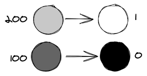
You can play the same game with colors. Imagine the r,g,b colors as values along the axes in 3D cartesian coordinates. 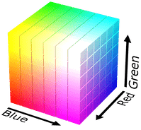
Color similarity can be measured as the distance between two points (r1, g1, b1) and (r2, g2, b2) in 3D cartesian space.
d = sqrt((r2-r1)² + (g2-g1)² + (b2-b1)²)
Humans, though, do not perceive the red, green, and blue shades the same way. So colors are usually weighted to better match human vision — red 30%, green 59%, and blue 11%. Better yet, use the CIELAB color space, which describes a color closer to how humans perceive color.
ΔE = sqrt(ΔL² + Δa² + Δb²)
So the distance in CIELAB space would more accurately depict the closeness of two colors (more on this).
Palette mapping is not enough
Take a moment to try the interactive demo at the top of this page with dithering OFF. You will notice that the output is not quite as attractive.
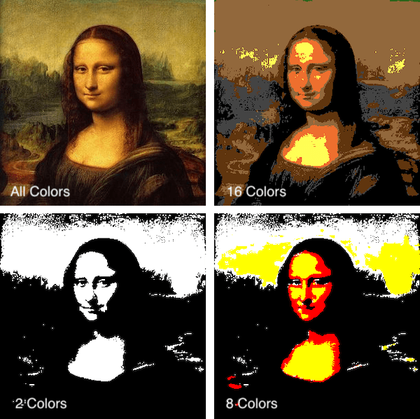
A one-to-one mapping of colors does the job, but we lose the character in the image. We can do better, and believe it or not, we do it by adding noise to the image.
When we approximated the colors from one palette to another, the difference in the color introduced in the pixel is called quantization error. Dithering is applying noise to the image to distribute these quantization errors.
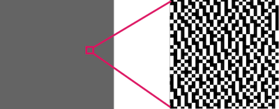
Take a simple example of gray rectangle (grayscale value 100). Mapping the rectangle to binary, every pixel in the rectangle will turn black because 100 is less than 128. But, what if, instead, we turn pixels black or white with such a density that the average gray level is maintained — at least to the human eye when looked at a distance.
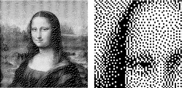
Error Diffusion Dithering
Two common ways dithering are Ordered and Error Diffusion. Ordered dithering is based on a fixed matrix and is localized — a pixel’s value does not influence the dithering of surrounding pixels. Read more about it here. In Error Diffusion dithering, the quantization error of a pixel is distributed to the surrounding pixels. Unlike Ordered dithering, Error Diffusion can work with any color palette, which is the main reason I’ll focus on it.
A popular version of Error Diffusion dithering is Floyd–Steinberg dithering. In this algorithm you go through one pixel at time — left to right, and top to bottom. For each pixel, we distribute the quantization error to the surrounding pixels that have not been processed yet. Floyd–Steinberg suggests that the error is distributed in fractions of 7/16, 1/16, 5/16, 3/16 in clockwise directions.
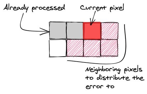
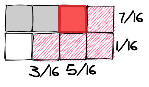
Let’s work on an example. Keeping it simple at first, a grayscale image to binary. Let’s say the current pixel value is 100, which gets resolved to 0 in binary. The quantization error for the pixel is 100 - 0 = 100. This error is now distributed to the surrounding pixels using the fractions defined above.
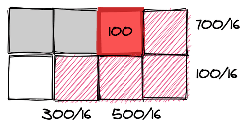
Moving on to the next pixel, the pixel to the right of the previous one. The value of this pixel is, say, 50. It also has the error from the previous pixel, so the effective value of this pixel is 50 + 700/16 ≅ 94. Now 94 also approximates to 0 with a quantization error of 94 which is further distributed to the following pixels.
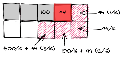
Dithering with color
The algorithm can now easily be extrapolated to the CIELAB color space. The quantization error is not a number anymore, but a tuple of individual difference in the LAB colors (ΔL, Δa, Δb). When distributing the error, each value of the tuple is multiplied by the associated fraction.
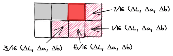
Note: Since writing this, people have suggested that dithering would work better in RGB space causing less hue shift. Finding the closest color using CIELAB color space but distribute the quantization error in RGB. I tested this and the color boundaries do look better but the image brightness seems to be affected as well. When working with binary images though, certain images created a banding effect around some color boundaries, which did not appear in CIELAB space.
Formalize the algorithm
Floyd–Steinberg dithering explained above can be formalized as follows:
for each y from top to bottom do
    for each x from left to right do
        oldpixel := pixel[x][y]
        newpixel := find_closest_palette_color(oldpixel)
        pixel[x][y] := newpixel
        quant_error := oldpixel - newpixel
        pixel[x + 1][y    ] := pixel[x + 1][y    ] + quant_error × 7 / 16
        pixel[x - 1][y + 1] := pixel[x - 1][y + 1] + quant_error × 3 / 16
        pixel[x    ][y + 1] := pixel[x    ][y + 1] + quant_error × 5 / 16
        pixel[x + 1][y + 1] := pixel[x + 1][y + 1] + quant_error × 1 / 16
Demo it again, good sir!
Take a moment to play with this interactive demo of Dithering (Yes, this is the same as the one on top of the post).
How I got here + Epilogue
I was trying to solve a problem where I could map images created by LegraJS to actual available Lego pieces — Figure out what Lego pieces one would need in what color. This led me to image color reduction and then to Dithering. I have since discovered that dithering is not the right solution for that use case… more on that later. But, it was fascinating to discover the process. I was aware of dithering but never got around to actually implementing it. Code for the TypeScript implementation I wrote can be found on the cielab-dither repo.
For the interactive demo on this page, I used this implementation and run the algorithm in a WebWorker. I wrapped the demo as a WebComponent and just drop the element wherever I needed in the blog post: <dither-view></dither-view>
Feel free to reach out to me on Twitter with any feedback or comments. Cheers!

_MBK_
Пикирующий бомбардировщик
-
#2
Ответ: Обьясните про алгоритм Error Difusion
Для начала давайте определимся — где вы этот самый Error diffusion видели? В какой конкретно программе? Исходя из этого можно продолжать обсуждение. А вообще, да, самый близкий из стандартных фотошоповских алгоритмов к стохастике — именно этот.
_MBK_
Пикирующий бомбардировщик
-
#4
Ответ: Обьясните про алгоритм Error Difusion
Ну если никакой другой стохастики в данном драйвере не предусмотрено, то это — лучшая стохастика из всех возможных для данного драйвера. )' '))'")
_MBK_
Пикирующий бомбардировщик
_MBK_
Пикирующий бомбардировщик
-
#9
Ответ: Обьясните про алгоритм Error Difusion
У ТС не полиграфия, а гравировка. А там, почему бы и нет?
From Wikipedia, the free encyclopedia
Error diffusion is a type of halftoning in which the quantization residual is distributed to neighboring pixels that have not yet been processed. Its main use is to convert a multi-level image into a binary image, though it has other applications.
Unlike many other halftoning methods, error diffusion is classified as an area operation, because what the algorithm does at one location influences what happens at other locations. This means buffering is required, and complicates parallel processing. Point operations, such as ordered dither, do not have these complications.
Error diffusion has the tendency to enhance edges in an image. This can make text in images more readable than in other halftoning techniques.

An error-diffused image
Early history[edit]
Richard Howland Ranger received United States patent 1790723 for his invention, «Facsimile system.» The patent, which issued in 1931, describes a system for transmitting images over telephone or telegraph lines, or by radio.[1] Ranger’s invention permitted continuous tone photographs to be converted first into black and white, then transmitted to remote locations, which had a pen moving over a piece of paper. To render black, the pen was lowered to the paper; to produce white, the pen was raised. Shades of gray were rendered by intermittently raising and lowering the pen, depending upon the luminance of the gray desired.
Ranger’s invention used capacitors to store charges, and vacuum tube comparators to determine when the present luminance, plus any accumulated error, was above a threshold (causing the pen to be raised) or below (causing the pen to be lowered). In this sense, it was an analog version of error diffusion.
Digital era[edit]
Floyd and Steinberg described a system for performing error diffusion on digital images based on a simple kernel:
![{frac {1}{16}}left[{begin{array}{ccccc}-&#&7\3&5&1end{array}}right]](https://wikimedia.org/api/rest_v1/media/math/render/svg/aef590317e58bf01da429ca7063b5a71e9e44327)
where « » denotes a pixel in the current row which has already been processed (hence diffusing error to it would be pointless), and «#» denotes the pixel currently being processed.
Nearly concurrently, J F Jarvis, C N Judice, and W H Ninke of Bell Labs disclosed a similar method which they termed «minimized average error» using a larger kernel: [2]
![{frac {1}{48}}left[{begin{array}{ccccc}-&-&#&7&5\3&5&7&5&3\1&3&5&3&1end{array}}right]](https://wikimedia.org/api/rest_v1/media/math/render/svg/2afcbcf36957fb6560391c4d1f12da577ec4a436)
Algorithm description[edit]
Error diffusion takes a monochrome or color image and reduces the number of quantization levels.[3] A popular application of error diffusion involves reducing the number of quantization states to just two per channel. This makes the image suitable for printing on binary printers such as black and white laser printers.
In the discussion which follows, it is assumed that the number of quantization states in the error diffused image is two per channel, unless otherwise stated.
One-dimensional error diffusion[edit]
The simplest form of the algorithm scans the image one row at a time and one pixel at a time. The current pixel is compared to a half-gray value. If it is above the value a white pixel is generated in the resulting image. If the pixel is below the half way brightness, a black pixel is generated. Different methods may be used if the target palette is not monochrome, such as thresholding with two values if the target palette is black, gray and white. The generated pixel is either full bright, or full black, so there is an error in the image. The error is then added to the next pixel in the image and the process repeats.
Two-dimensional error diffusion[edit]
One dimensional error diffusion tends to have severe image artifacts that show up as distinct vertical lines. Two dimensional error diffusion reduces the visual artifacts. The simplest algorithm is exactly like one dimensional error diffusion, except half the error is added to the next pixel, and half of the error is added to the pixel on the next line below.
The kernel is:
![{displaystyle {frac {1}{2}}left[{begin{array}{cc}#&1\1&0end{array}}right]}](https://wikimedia.org/api/rest_v1/media/math/render/svg/2fc09e179d72b9c6edd48de013aba58a6b6add32)
where «#» denotes the pixel currently being processed.
Further refinement can be had by dispersing the error further away from the current pixel, as in the matrices given above in Digital era. The sample image at the start of this article is an example of two dimensional error diffusion.
Color error diffusion[edit]
The same algorithms may be applied to each of the red, green, and blue (or cyan, magenta, yellow, black) channels of a color image to achieve a color effect on printers such as color laser printers that can only print single color values.
However, better visual results may be obtained by first converting the color channels into a perceptive color model that will separate lightness, hue and saturation channels, so that a higher weight for error diffusion will be given to the lightness channel, than to the hue channel. The motivation for this conversion is that human vision better perceives small differences of lightness in small local areas, than similar differences of hue in the same area, and even more than similar differences of saturation on the same area.
For example, if there is a small error in the green channel that cannot be represented, and another small error in the red channel in the same case, the properly weighted sum of these two errors may be used to adjust a perceptible lightness error, that can be represented in a balanced way between all three color channels (according to their respective statistical contribution to the lightness), even if this produces a larger error for the hue when converting the green channel. This error will be diffused in the neighboring pixels.
In addition, gamma correction may be needed on each of these perceptive channels, if they don’t scale linearly with the human vision, so that error diffusion can be accumulated linearly to these gamma-corrected linear channels, before computing the final color channels of the rounded pixel colors, using a reverse conversion to the native non gamma-corrected image format and from which the new residual error will be computed and converted again to be distributed to the next pixels.
Error diffusion with several gray levels[edit]
Error Diffusion may also be used to produce output images with more than two levels (per channel, in the case of color images). This has application in displays and printers which can produce 4, 8, or 16 levels in each image plane, such as electrostatic printers and displays in compact mobile telephones. Rather than use a single threshold to produce binary output, the closest permitted level is determined, and the error, if any, is diffused as described above.
Printer considerations[edit]
Most printers overlap the black dots slightly so there is not an exact one-to-one relationship to dot frequency (in dots per unit area) and lightness. Tone scale linearization may be applied to the source image to get the printed image to look correct.
Edge enhancement versus lightness preservation[edit]
When an image has a transition from light to dark the error diffusion algorithm tends to
make the next generated pixel be black. Dark to light transitions tend to result in the next
generated pixel being white. This causes an edge enhancement effect at the expense of gray level reproduction accuracy. This results in error diffusion having a higher apparent resolution than other halftone methods. This is especially beneficial with images with text in them such as the typical facsimile.
This effect shows fairly well in the picture at the top of this article. The grass detail and the text on the sign is well preserved,
and the lightness in the sky, containing little detail. A cluster-dot halftone image of the same resolution would be much less sharp.
See also[edit]
- Floyd–Steinberg dithering
- Halftone
References[edit]
- ^ Richard Howland Ranger, Facsimile system. United States Patent 1790723, issued 3 February 1931.
- ^ J F Jarvis, C N Judice, and W H Ninke, A survey of techniques for the display of continuous tone pictures on bilevel displays. Computer Graphics and Image Processing, 5:1:13–40 (1976).
- ^ «Error Diffusion — an overview | ScienceDirect Topics». www.sciencedirect.com. Retrieved 2022-05-09.
External links[edit]
- Error diffusion in Matlab
I always loved the visual aesthetic of dithering but never knew how it’s done. So I did some research. This article may contain traces of nostalgia and none of Lena.
How did I get here? (You can skip this)
I am late to the party, but I finally played “Return of the Obra Dinn”, the most recent game by Lucas Pope of “Papers Please” fame. Obra Dinn is a story puzzler that I can only recommend, but what piqued my curiosity as a software engineer is that it is a 3D game (using the Unity game engine) but rendered using only 2 colors with dithering. Apparently, this has been dubbed “Ditherpunk”, and I love that.
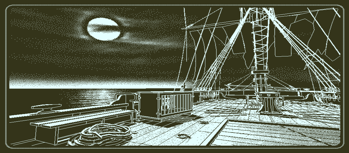
Dithering, so my original understanding, was a technique to place pixels using only a few colors from a palette in a clever way to trick your brain into seeing many colors. Like in the picture, where you probably feel like there are multiple brightness levels when in fact there’s only two: Full brightness and black.
The fact that I have never seen a 3D game with dithering like this probably stems from the fact that color palettes are mostly a thing of the past. You may remember running Windows 95 with 16 colors and playing games like “Monkey Island” on it.
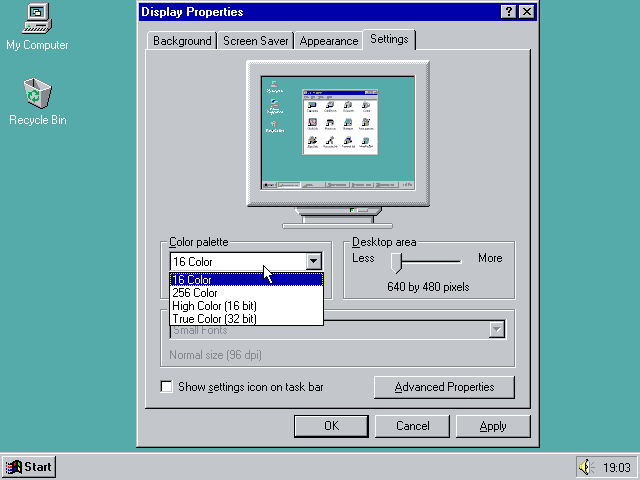
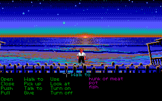
For a long time now, however, we have had 8 bits per channel per pixel, allowing each pixel on your screen to assume one of 16 million colors. With HDR and wide gamut on the horizon, things are moving even further away to ever requiring any form of dithering. And yet Obra Dinn used it anyway and rekindled a long forgotten love for me. Knowing a tiny bit about dithering from my work on Squoosh, I was especially impressed with Obra Dinn’s ability to keep the dithering stable while I moved and rotated the camera through 3D space and I wanted to understand how it all worked.
As it turns out, Lucas Pope wrote a forum post where he explains which dithering techniques he uses and how he applies them to 3D space. He put extensive work into making the dithering stable when camera movements occur. Reading that forum post kicked me down the rabbit hole, which this blog post tries to summarize.
Dithering
What is Dithering?
According to Wikipedia, “Dither is an intentionally applied form of noise used to randomize quantization error”, and is a technique not only limited to images. It is actually a technique used to this day on audio recordings, but that is yet another rabbit hole to fall into another time. Let’s dissect that definition in the context of images. First up: Quantization.
Quantization
Quantization is the process of mapping a large set of values to a smaller, usually finite, set of values. For the remainder of this article, I am going to use two images as examples:
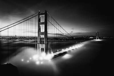
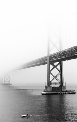
Both black-and-white photos use 256 different shades of gray. If we wanted to use fewer colors — for example just black and white to achieve monochromaticity — we have to change every pixel to be either pure black or pure white. In this scenario, the colors black and white are called our “color palette” and the process of changing pixels that do not use a color from the palette is called “quantization”. Because not all colors from the original images are in the color palette, this will inevitably introduce an error called the “quantization error”. The naïve solution is to quantizer each pixel to the color in the palette that is closest to the pixel’s original color.
Note: Defining which colors are “close to each other” is open to interpretation and depends on how you measure the distance between two colors. I suppose ideally we’d measure distance in a psycho-visual way, but most of the articles I found simply used the euclidian distance in the RGB cube, i.e. Δred2+Δgreen2+Δblue2sqrt{Deltatext{red}^2 + Deltatext{green}^2 + Deltatext{blue}^2}.
With our palette only consisting of black and white, we can use the brightness of a pixel to decide which color to quantize to. A brightness of 0 means black, a brightness of 1 means white, everything else is in-between, ideally correlating with human perception such that a brightness of 0.5 is a nice mid-gray. To quantize a given color, we only need to check if the color’s brightness is greater or less than 0.5 and quantize to white and black respectively. Applying this quantization to the image above yields an… unsatisfying result.
grayscaleImage.mapSelf(brightness =>
  brightness > 0.5
    ? 1.0
    : 0.0
);
Note: The code samples in this article are real but built on top of a helper class
GrayImageF32N0F8I wrote for the demo of this article. It’s similar to the web’sImageData, but usesFloat32Array, only has one color channel, represents values between 0.0 and 1.0 and has a whole bunch of helper functions. The source code is available in the lab.
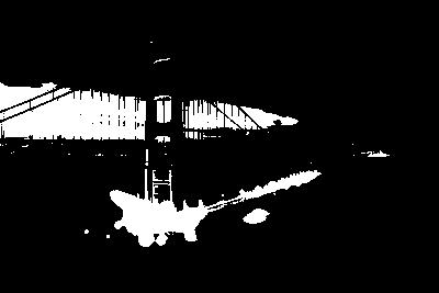
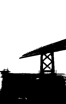
Gamma
I had finished writing this article and just wanted to “quickly” look what a black-to-white gradient looks like with the different dithering algorithms. The results showed me that I failed to consider the thing that always becomes a problem when working with images: color spaces. I had written the sentence “ideally correlating with human perception” without actually following it myself.
My demo is implemented using web technologies, most notably <canvas> and ImageData, which are — at the time of writing — specified to use sRGB. It’s an old color space specification (from 1996) whose value-to-color mapping was modeled to mirror the behavior of CRT monitors. While barely anyone uses CRTs these days, it’s still considered the “safe” color space that gets correctly displayed on every display. As such, it is the default on the web platform. However, sRGB is not linear, meaning that (0.5,0.5,0.5)(0.5, 0.5, 0.5) in sRGB is not the color a human sees when you mix 50% of (0,0,0)(0, 0, 0) and (1,1,1)(1, 1, 1). Instead, it’s the color you get when you pump half the power of full white through your Cathode-Ray Tube (CRT).
![]()
Warning: I set
image-rendering: pixelated;on most of the images in this article. This allows you to zoom in and truly see the pixels. However, on devices with fractiondevicePixelRatio, this might introduce artifacts. If in doubt, open the image separate in a new tab.
As this image shows, the dithered gradient gets bright way too quickly. If we want 0.5 be the color in the middle of pure black and white (as perceived by a human), we need to convert from sRGB to linear RGB space, which can be done with a process called “gamma correction”. Wikipedia lists the following formulas to convert between sRGB and linear RGB.
srgbToLinear(b)={b12.92b≤0.04045(b+0.0551.055)γotherwiselinearToSrgb(b)={12.92⋅bb≤0.00313081.055⋅b1γ−0.055otherwise(γ=2.4)begin{array}{rcl}
text{srgbToLinear}(b) & = & left{begin{array}{ll}
frac{b}{12.92} & b le 0.04045 \
left( frac{b + 0.055}{1.055}right)^{gamma} & text{otherwise}
end{array}right.\
text{linearToSrgb}(b) & = & left{begin{array}{ll}
12.92cdot b & b le 0.0031308 \
1.055 cdot b^frac{1}{gamma} — 0.055 & text{otherwise}
end{array}right.\
(gamma = 2.4)
end{array}\
With these conversions in place, dithering produces (more) accurate results:
![]()
Random noise
Back to Wikipedia’s definition of dithering: “Intentionally applied form of noise used to randomize quantization error”. We got the quantization down, and now it says to add noise. Intentionally.
Instead of quantizing each pixel directly, we add noise with a value between -0.5 and 0.5 to each pixel. The idea is that some pixels will now be quantized to the “wrong” color, but how often that happens depends on the pixel’s original brightness. Black will always remain black, white will always remain white, a mid-gray will be dithered to black roughly 50% of the time. Statistically, the overall quantization error is reduced and our brains are eager to do the rest and help you see the, uh, big picture.
grayscaleImage.mapSelf(brightness =>
  brightness + (Math.random() - 0.5) > 0.5
    ? 1.0
    : 0.0
);

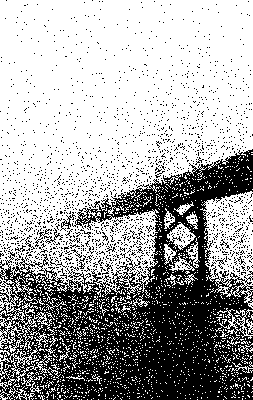
I found this quite surprising! It is by no means good — video games from the 90s have shown us that we can do better — but this is a very low effort and quick way to get more detail into a monochrome image. And if I was to take “dithering” literally, I’d end my article here. But there’s more…
Ordered Dithering
Instead of talking about what kind of noise to add to an image before quantizing it, we can also change our perspective and talk about adjusting the quantization threshold.
// Adding noise
grayscaleImage.mapSelf(brightness =>
  brightness + Math.random() - 0.5 > 0.5
    ? 1.0
    : 0.0
);

// Adjusting the threshold
grayscaleImage.mapSelf(brightness =>
  brightness > Math.random()
    ? 1.0
    : 0.0
);
In the context of monochrome dithering, where the quantization threshold is 0.5, these two approaches are equivalent:
brightness+rand()−0.5>0.5⇔brightness>1.0−rand()⇔brightness>rand()begin{array}
{} & mathrm{brightness} + mathrm{rand}() — 0.5 & > & 0.5 \
Leftrightarrow &
mathrm{brightness} & > & 1.0 — mathrm{rand}() \
Leftrightarrow & mathrm{brightness} &>& mathrm{rand}()
end{array}
The upside of this approach is that we can talk about a “threshold map”. Threshold maps can be visualized to make it easier to reason about why a resulting image looks the way it does. They can also be precomputed and reused, which makes the dithering process deterministic and parallelizable per pixel. As a result, the dithering can happen on the GPU as a shader. This is what Obra Dinn does! There are a couple of different approaches to generating these threshold maps, but all of them introduce some kind of order to the noise that is added to the image, hence the name “ordered dithering”.
The threshold map for the random dithering above, literally a map full of random thresholds, is also called “white noise”. The name comes from a term in signal processing where every frequency has the same intensity, just like in white light.
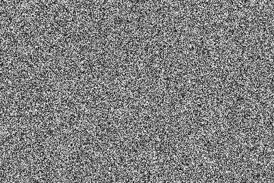
Bayer Dithering
“Bayer dithering” uses a Bayer matrix as the threshold map. They are named after Bryce Bayer, inventor of the Bayer filter, which is in use to this day in digital cameras. Each pixel on the sensor can only detect brightness, but by cleverly arranging colored filters in front of the individual pixels, we can reconstruct color images through demosaicing. The pattern for the filters is the same pattern used in Bayer dithering.
Bayer matrices come in various sizes which I ended up calling “levels”. Bayer Level 0 is 2×22 times 2 matrix. Bayer Level 1 is a 4×44
times 4 matrix. Bayer Level nn is a 2n+1×2n+12^{n+1} times 2^{n+1} matrix. A level nn matrix can be recursively calculated from level n−1n-1 (although Wikipedia also lists an per-cell algorithm). If your image happens to be bigger than your bayer matrix, you can tile the threshold map.
Bayer(0)=(0231)begin{array}{rcl}
text{Bayer}(0) &
= &
left(
begin{array}{cc}
0 & 2 \
3 & 1 \
end{array}
right) \
end{array}
Bayer(n)=(4⋅Bayer(n−1)+04⋅Bayer(n−1)+24⋅Bayer(n−1)+34⋅Bayer(n−1)+1)begin{array}{c}
text{Bayer}(n) = \
left(
begin{array}{cc}
4 cdot text{Bayer}(n-1) + 0 & 4 cdot text{Bayer}(n-1) + 2 \
4 cdot text{Bayer}(n-1) + 3 & 4 cdot text{Bayer}(n-1) + 1 \
end{array}
right)
end{array}
A level nn Bayer matrix contains the numbers 00 to 22n+22^{2n+2}. Once you normalize the Bayer matrix, i.e. divide by 22n+22^{2n+2}, you can use it as a threshold map:
const bayer = generateBayerLevel(level);
grayscaleImage.mapSelf((brightness, { x, y }) =>
  brightness > bayer.valueAt(x, y, { wrap: true })
    ? 1.0
    : 0.0
);
One thing to note: Bayer dithering using matrices as defined above will render an image lighter than it originally was. For example: An area where every pixel has a brightness of 1255=0.4%frac{1}{255} = 0.4%, a level 0 Bayer matrix of size 2×22times2 will make one out of the four pixels white, resulting in an average brightness of 25%25%. This error gets smaller with higher Bayer levels, but a fundamental bias remains.
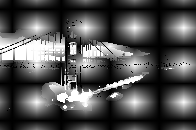
In our dark test image, the sky is not pure black and made significantly brighter when using Bayer Level 0. While it gets better with higher levels, an alternative solution is to flip the bias and make images render darker by inverting the way we use the Bayer matrix:
const bayer = generateBayerLevel(level);
grayscaleImage.mapSelf((brightness, { x, y }) =>
  //           👇
  brightness > 1 - bayer.valueAt(x, y, { wrap: true })
    ? 1.0
    : 0.0
);
I have used the original Bayer definition for the light image and the inverted version for the dark image. I personally found Level 1 and 3 the most aesthetically pleasing.

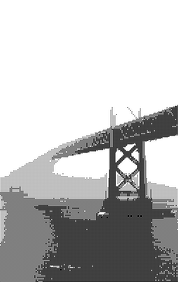


Blue noise
Both white noise and Bayer dithering have drawbacks, of course. Bayer dithering, for example, is very structured and will look quite repetitive, especially at lower levels. White noise is random, meaning that there inevitably will be clusters of bright pixels and voids of darker pixels in the threshold map. This can be made more obvious by squinting or, if that is too much work for you, through blurring the threshold map algorithmically. These clusters and voids can affect the output of the dithering process negatively. If darker areas of the image fall into one of the clusters, details will get lost in the dithered output (and vice-versa for brighter areas falling into voids).
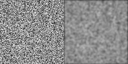
There is a variant of noise called “blue noise”, that addresses this issue. It is called blue noise because higher frequencies have higher intensities compared to the lower frequencies, just like blue light. By removing or dampening the lower frequencies, cluster and voids become less pronounced. Blue noise dithering is just as fast to apply to an image as white noise dithering — it’s just a threshold map in the end — but generating blue noise is a bit harder and expensive.
The most common algorithm to generate blue noise seems to be the “void-and-cluster method” by Robert Ulichney. Here is the original whitepaper. I found the way the algorithm is described quite unintuitive and, now that I have implemented it, I am convinced it is explained in an unnecessarily abstract fashion. But it is quite clever!
The algorithm is based on the idea that you can find a pixel that is part of cluster or a void by applying a Gaussian Blur to the image and finding the brightest (or darkest) pixel in the blurred image respectively. After initializing a black image with a couple of randomly placed white pixels, the algorithm proceeds to continuously swap cluster pixels and void pixels to spread the white pixels out as evenly as possible. Afterwards, every pixel gets a number between 0 and n (where n is the total number of pixels) according to their importance for forming clusters and voids. For more details, see the paper.
My implementation works fine but is not very fast, as I didn’t spend much time optimizing. It takes about 1 minute to generate a 64×64 blue noise texture on my 2018 MacBook, which is sufficient for these purposes. If something faster is needed, a promising optimization would be to apply the Gaussian Blur not in the spatial domain but in the frequency domain instead.
Excursion: Of course knowing this nerd-sniped me into implementing it. The reason this optimization is so promising is because convolution (which is the underlying operation of a Gaussian blur) has to loop over each field of the Gaussian kernel for each pixel in the image. However, if you convert both the image as well as the Gaussian kernel to the frequency domain (using one of the many Fast Fourier Transform algorithms), convolution becomes an element-wise multiplication. Since my targeted blue noise size is a power of two, I could implement the well-explored in-place variant of the Cooley-Tukey FFT algorithm. After some initial hickups, it did end up cutting the blue noise generation time by 50%. I still wrote pretty garbage-y code, so there’s a lot more to room for optimizations.
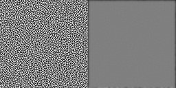
As blue noise is based on a Gaussian Blur, which is calculated on a torus (a fancy way of saying that Gaussian blur wraps around at the edges), blue noise will also tile seamlessly. So we can use the 64×64 blue noise and repeat it to cover the entire image. Blue noise dithering has a nice, even distribution without showing any obvious patterns, balancing rendering of details and organic look.


Error diffusion
All the previous techniques rely on the fact that quantization errors will statistically even out because the thresholds in the threshold maps are uniformly distributed. A different approach to quantization is the concept of error diffusion, which is most likely what you have read about if you have ever researched image dithering before. In this approach we don’t just quantize and hope that on average the quantization error remains negligible. Instead, we measure the quantization error and diffuse the error onto neighboring pixels, influencing how they will get quantized. We are effectively changing the image we want to dither as we go along. This makes the process inherently sequential.
Foreshadowing: One big advantage of error diffusion algorithms that we won’t touch on in this post is that they can handle arbitrary color palettes, while ordered dithering requires your color palette to be evenly spaced. More on that another time.
Almost all error diffusion ditherings that I am going to look at use a “diffusion matrix”, which defines how the quantization error from the current pixel gets distributed across the neighboring pixels. For these matrices it is often assumed that the image’s pixels are traversed top-to-bottom, left-to-right — the same way us westerners read text. This is important as the error can only be diffused to pixels that haven’t been quantized yet. If you find yourself traversing an image in a different order than the diffusion matrix assumes, flip the matrix accordingly.
“Simple” 2D error diffusion
The naïve approach to error diffusion shares the quantization error between the pixel below the current one and the one to the right, which can be described with the following matrix:
(∗0.50.50)left(begin{array}{cc}
* & 0.5 \
0.5 & 0 \
end{array}
right)
The diffusion algorithm visits each pixel in the image (in the right order!), quantizes the current pixel and measures the quantization error. Note that the quantization error is signed, i.e. it can be negative if the quantization made the pixel brighter than the original brightness value. We then add fractions of the quantization error to neighboring pixels as specified by the matrix. Rinse and repeat.
This animation is supposed to visualize the algorithm, but won’t be able to show that the dithered result resembles the original. 4×4 pixels are hardly enough do diffuse and average out quantization errors. But it does show that if a pixel is made brighter during quantization, neighboring pixels will be made darker to make up for it (and vice-versa).


However, the simplicity of the diffusion matrix is prone to generating patterns, like the line-like patterns you can see in the test images above.
Floyd-Steinberg
Floyd-Steinberg is arguably the most well-known error diffusion algorithm, if not even the most well-known dithering algorithm. It uses a more elaborate diffusion matrix to distribute the quantization error to all directly neighboring, unvisited pixels. The numbers are carefully chosen to prevent repeating patterns as much as possible.
116⋅(∗7351)frac{1}{16} cdot left(begin{array}
{} & * & 7 \
3 & 5 & 1 \
end{array}
right)
Floyd-Steinberg is a big improvement as it prevents a lot of patterns from forming. However, larger areas with little texture can still end up looking a bit unorganic.


Jarvis-Judice-Ninke
Jarvis, Judice and Ninke take an even bigger diffusion matrix, distributing the error to more pixels than just immediately neighboring ones.
148⋅(∗753575313531)frac{1}{48} cdot left(begin{array}
{} & {} & * & 7 & 5 \
3 & 5 & 7 & 5 & 3 \
1 & 3 & 5 & 3 & 1 \
end{array}
right)
Using this diffusion matrix, patterns are even less likely to emerge. While the test images still show some line like patterns, they are much less distracting now.

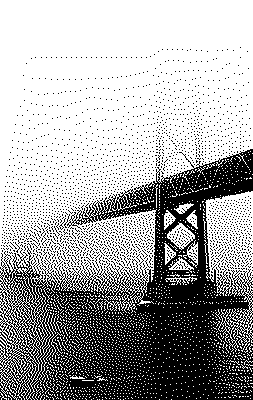
Atkinson Dither
Atkinson dithering was developed at Apple by Bill Atkinson and gained notoriety on on early Macintosh computers.
18⋅(∗111111)frac{1}{8} cdot left(begin{array}{}
& * & 1 & 1 \
1 & 1 & 1 & \
& 1 & & \
end{array}
right)
It’s worth noting that the Atkinson diffusion matrix contains six ones, but is normalized using 18frac{1}{8}, meaning it doesn’t diffuse the entire error to neighboring pixels, increasing the perceived contrast of the image.
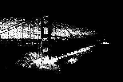

Riemersma Dither
To be completely honest, the Riemersma dither is something I stumbled upon by accident. I found an in-depth article while I was researching the other dithering algorithms. It doesn’t seem to be widely known, but I really like the way it looks and the concept behind it. Instead of traversing the image row-by-row it traverses the image with a Hilbert curve. Technically, any space-filling curve would do, but the Hilbert curve came recommended and is rather easy to implement using generators. Through this it aims to take the best of both ordered dithering and error diffusion dithering: Limiting the number of pixels a single pixel can influence together with the organic look (and small memory footprint).
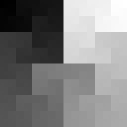
The Hilbert curve has a “locality” property, meaning that the pixels that are close together on the curve are also close together in the picture. This way we don’t need to use an error diffusion matrix but rather a diffusion sequence of length nn. To quantize the current pixel, the last nn quantization errors are added to the current pixel with weights given in the diffusion sequence. In the article they use an exponential falloff for the weights — the previous pixel’s quantization error getting a weight of 1, the oldest quantization error in the list a small, chosen weight rr. This results in the following formula for the iith weight:
weight[i]=r−in−1text{weight}[i] = r^{-frac{i}{n-1}}
The article recommends r=116r = frac{1}{16} and a minimum list length of n=16n = 16, but for my test image I found r=18r = frac{1}{8} and n=32n = 32 to be better looking.

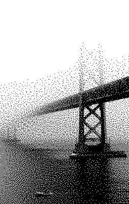
Riemersma dither with r=18r = frac{1}{8} and n=32n = 32.
The dithering looks extremely organic, almost as good as blue noise dithering. At the same time it is easier to implement than both of the previous ones. It is, however, still an error diffusion dithering algorithm, meaning it is sequential and not suitable to run on a GPU.
💛 Blue noise, Bayer & Riemersma
As a 3D game, Obra Dinn had to use ordered dithering to be able to run it as a shader. It uses both Bayer dithering and blue noise dithering which I also think are the most aesthetically pleasing choices. Bayer dithering shows a bit more structure while blue noise looks very natural and organic. I am also particularly fond of the Riemersma dither and I want to explore how it holds up when there are multiple colors in the palette.
Obra Dinn uses blue noise dithering for most of the environment. People and other objects of interest are dithered using Bayer, which forms a nice visual contrast and makes them stand out without breaking the games overall aesthetic. Again, more on his reasoning as well his solution to handling camera movement in his forum post.
If you want to try different dithering algorithms on one of your own images, take a look at my demo that I wrote to generate all the images in this blog post. Keep in mind that these are not the fastest. If you decide to throw your 20 megapixel camera JPEG at this, it will take a while.
Note: It seems I am hitting a de-opt in Safari. My blue noise generator takes ~30 second in Chrome, but takes >20 minutes Safari. It is considerably quicker in Safari Tech Preview.
I am sure this super niche, but I enjoyed this rabbit hole. If you have any opinions or experiences with dithering, I’d love to hear them.
Thanks & other sources
Thanks to Lucas Pope for his games and the visual inspiration.
Thanks to Christoph Peters for his excellent article on blue noise generation.
Specifies the color palette to apply to the indexed-color
image. There are 10 color palettes available:
Exact
Creates a panel using the exact colors that appear in the
RGB image—an option available only if the image uses 256 or fewer
colors. Because the image’s panel contains all of the colors in
the image, there is no dithering.
System (Mac OS)
Uses the Mac OS default 8‑bit panel, which is based on a uniform
sampling of RGB colors.
System (Windows)
Uses the Windows system’s default 8‑bit panel, which is based
on a uniform sampling of RGB colors.
Web
Uses the 216 colors that web browsers, regardless of platform,
use to display images on a monitor limited to 256 colors. Use this
option to avoid browser dither when images are viewed on a monitor
display limited to 256 colors.
Uniform
Creates a panel by uniformly sampling colors from the RGB
color cube. For example, if Photoshop Elements takes
6 evenly spaced color levels, each of red, green, and blue, the
combination produces a uniform panel of 216 colors (6 cubed = 6
x 6 x 6 = 216). The total number of colors displayed in an image
corresponds to the nearest perfect cube (8, 27, 64, 125, or 216)
that is less than the value in the Colors text box.
Local or Master Perceptual
Creates a custom panel by giving priority to colors to which
the human eye has greater sensitivity. Local Perceptual applies
the panel to individual images; Master Perceptual applies the selected
panel to multiple images (for example, for multimedia production).
Local or Master Selective
Creates a color table similar to the Perceptual color table,
but favoring broad areas of color and the preservation of web colors.
This option usually produces images with the greatest color integrity.
Local Selective applies the panel to individual images; Master Selective
applies the selected panel to multiple images (for example, for
multimedia production).
Local or Master Adaptive
Creates a panel by sampling the colors from the spectrum
appearing most often in the image. For example, an RGB image with only
the colors green and blue produces a panel made primarily of greens
and blues. Most images concentrate colors in particular areas of
the spectrum. To control a panel more precisely, first select a
part of the image that contains the colors you want to emphasize. Photoshop Elements weights the conversion toward these
colors. Local Adaptive applies the panel to individual images; Master Adaptive
applies the selected panel to multiple images (for example, for
multimedia production).
Custom
Creates a custom panel by using the Color Table dialog box.
Either edit the color table and save it for later use, or click
Load to load a previously created color table. This option also
displays the current Adaptive panel, which is useful for previewing
the colors most often used in the image.
Previous
Uses the custom panel from the previous conversion, making
it easy to convert several images with the same custom panel.