This article is about the computer algorithm. For the biological process, see neural backpropagation.
Backpropagation can also refer to the way the result of a playout is propagated up the search tree in Monte Carlo tree search.
In machine learning, backpropagation (backprop,[1] BP) is a widely used algorithm for training feedforward artificial neural networks. Generalizations of backpropagation exist for other artificial neural networks (ANNs), and for functions generally. These classes of algorithms are all referred to generically as «backpropagation».[2] In fitting a neural network, backpropagation computes the gradient of the loss function with respect to the weights of the network for a single input–output example, and does so efficiently, unlike a naive direct computation of the gradient with respect to each weight individually. This efficiency makes it feasible to use gradient methods for training multilayer networks, updating weights to minimize loss; gradient descent, or variants such as stochastic gradient descent, are commonly used. The backpropagation algorithm works by computing the gradient of the loss function with respect to each weight by the chain rule, computing the gradient one layer at a time, iterating backward from the last layer to avoid redundant calculations of intermediate terms in the chain rule; this is an example of dynamic programming.[3]
The term backpropagation strictly refers only to the algorithm for computing the gradient, not how the gradient is used; however, the term is often used loosely to refer to the entire learning algorithm, including how the gradient is used, such as by stochastic gradient descent.[4] Backpropagation generalizes the gradient computation in the delta rule, which is the single-layer version of backpropagation, and is in turn generalized by automatic differentiation, where backpropagation is a special case of reverse accumulation (or «reverse mode»).[5] The term backpropagation and its general use in neural networks was announced in Rumelhart, Hinton & Williams (1986a), then elaborated and popularized in Rumelhart, Hinton & Williams (1986b), but the technique was independently rediscovered many times, and had many predecessors dating to the 1960s; see § History.[6] A modern overview is given in the deep learning textbook by Goodfellow, Bengio & Courville (2016).[7]
Overview[edit]
Backpropagation computes the gradient in weight space of a feedforward neural network, with respect to a loss function. Denote:
 : input (vector of features)
- : target output
- For classification, output will be a vector of class probabilities (e.g., , and target output is a specific class, encoded by the one-hot/dummy variable (e.g., ).
- For classification, output will be a vector of class probabilities (e.g.,
- : loss function or «cost function»[a]
- For classification, this is usually cross entropy (XC, log loss), while for regression it is usually squared error loss (SEL).
- : the number of layers
- : the weights between layer and , where is the weight between the -th node in layer and the -th node in layer [b]
- : activation functions at layer
- For classification the last layer is usually the logistic function for binary classification, and softmax (softargmax) for multi-class classification, while for the hidden layers this was traditionally a sigmoid function (logistic function or others) on each node (coordinate), but today is more varied, with rectifier (ramp, ReLU) being common.


In the derivation of backpropagation, other intermediate quantities are used; they are introduced as needed below. Bias terms are not treated specially, as they correspond to a weight with a fixed input of 1. For the purpose of backpropagation, the specific loss function and activation functions do not matter, as long as they and their derivatives can be evaluated efficiently. Traditional activation functions include but are not limited to sigmoid, tanh, and ReLU. Since, swish,[8] mish,[9] and other activation functions were proposed as well.
The overall network is a combination of function composition and matrix multiplication:

For a training set there will be a set of input–output pairs,  . For each input–output pair
  in the training set, the loss of the model on that pair is the cost of the difference between the predicted output
  and the target output
  :
:

Note the distinction: during model evaluation, the weights are fixed, while the inputs vary (and the target output may be unknown), and the network ends with the output layer (it does not include the loss function). During model training, the input–output pair is fixed, while the weights vary, and the network ends with the loss function.
Backpropagation computes the gradient for a fixed input–output pair , where the weights  can vary. Each individual component of the gradient,
  can be computed by the chain rule; however, doing this separately for each weight is inefficient. Backpropagation efficiently computes the gradient by avoiding duplicate calculations and not computing unnecessary intermediate values, by computing the gradient of each layer – specifically, the gradient of the weighted input of each layer, denoted by
  – from back to front.
Informally, the key point is that since the only way a weight in  affects the loss is through its effect on the next layer, and it does so linearly, are the only data you need to compute the gradients of the weights at layer
  , and then you can compute the previous layer
  and repeat recursively. This avoids inefficiency in two ways. Firstly, it avoids duplication because when computing the gradient at layer , you do not need to recompute all the derivatives on later layers
  each time. Secondly, it avoids unnecessary intermediate calculations because at each stage it directly computes the gradient of the weights with respect to the ultimate output (the loss), rather than unnecessarily computing the derivatives of the values of hidden layers with respect to changes in weights
  .
.
Backpropagation can be expressed for simple feedforward networks in terms of matrix multiplication, or more generally in terms of the adjoint graph.
Matrix multiplication[edit]
For the basic case of a feedforward network, where nodes in each layer are connected only to nodes in the immediate next layer (without skipping any layers), and there is a loss function that computes a scalar loss for the final output, backpropagation can be understood simply by matrix multiplication.[c] Essentially, backpropagation evaluates the expression for the derivative of the cost function as a product of derivatives between each layer from right to left – «backwards» – with the gradient of the weights between each layer being a simple modification of the partial products (the «backwards propagated error»).
Given an input–output pair  , the loss is:

To compute this, one starts with the input  and works forward; denote the weighted input of each hidden layer as
  and the output of hidden layer as the activation
  . For backpropagation, the activation as well as the derivatives
  (evaluated at ) must be cached for use during the backwards pass.
The derivative of the loss in terms of the inputs is given by the chain rule; note that each term is a total derivative, evaluated at the value of the network (at each node) on the input :

where  is a Hadamard product, that is an element-wise product.
These terms are: the derivative of the loss function;[d] the derivatives of the activation functions;[e] and the matrices of weights:[f]

The gradient  is the transpose of the derivative of the output in terms of the input, so the matrices are transposed and the order of multiplication is reversed, but the entries are the same:

Backpropagation then consists essentially of evaluating this expression from right to left (equivalently, multiplying the previous expression for the derivative from left to right), computing the gradient at each layer on the way; there is an added step, because the gradient of the weights isn’t just a subexpression: there’s an extra multiplication.
Introducing the auxiliary quantity for the partial products (multiplying from right to left), interpreted as the «error at level » and defined as the gradient of the input values at level :

Note that is a vector, of length equal to the number of nodes in level ; each component is interpreted as the «cost attributable to (the value of) that node».
The gradient of the weights in layer is then:

The factor of  is because the weights between level
  and affect level proportionally to the inputs (activations): the inputs are fixed, the weights vary.
The can easily be computed recursively, going from right to left, as:

The gradients of the weights can thus be computed using a few matrix multiplications for each level; this is backpropagation.
Compared with naively computing forwards (using the for illustration):

there are two key differences with backpropagation:
- Computing in terms of avoids the obvious duplicate multiplication of layers and beyond.
- Multiplying starting from – propagating the error backwards – means that each step simply multiplies a vector () by the matrices of weights and derivatives of activations . By contrast, multiplying forwards, starting from the changes at an earlier layer, means that each multiplication multiplies a matrix by a matrix. This is much more expensive, and corresponds to tracking every possible path of a change in one layer forward to changes in the layer (for multiplying by , with additional multiplications for the derivatives of the activations), which unnecessarily computes the intermediate quantities of how weight changes affect the values of hidden nodes.


Adjoint graph[edit]
|
This section needs expansion. You can help by adding to it. (November 2019) |
For more general graphs, and other advanced variations, backpropagation can be understood in terms of automatic differentiation, where backpropagation is a special case of reverse accumulation (or «reverse mode»).[5]
Intuition[edit]
Motivation[edit]
The goal of any supervised learning algorithm is to find a function that best maps a set of inputs to their correct output. The motivation for backpropagation is to train a multi-layered neural network such that it can learn the appropriate internal representations to allow it to learn any arbitrary mapping of input to output.[10]
Learning as an optimization problem[edit]
To understand the mathematical derivation of the backpropagation algorithm, it helps to first develop some intuition about the relationship between the actual output of a neuron and the correct output for a particular training example. Consider a simple neural network with two input units, one output unit and no hidden units, and in which each neuron uses a linear output (unlike most work on neural networks, in which mapping from inputs to outputs is non-linear)[g] that is the weighted sum of its input.

A simple neural network with two input units (each with a single input) and one output unit (with two inputs)
Initially, before training, the weights will be set randomly. Then the neuron learns from training examples, which in this case consist of a set of tuples  where
where  and
and  are the inputs to the network and t is the correct output (the output the network should produce given those inputs, when it has been trained). The initial network, given and , will compute an output y that likely differs from t (given random weights). A loss function
  is used for measuring the discrepancy between the target output t and the computed output y. For regression analysis problems the squared error can be used as a loss function, for classification the categorical crossentropy can be used.
As an example consider a regression problem using the square error as a loss:

where E is the discrepancy or error.
Consider the network on a single training case:  . Thus, the input and are 1 and 1 respectively and the correct output, t is 0. Now if the relation is plotted between the network’s output y on the horizontal axis and the error E on the vertical axis, the result is a parabola. The minimum of the parabola corresponds to the output y which minimizes the error E. For a single training case, the minimum also touches the horizontal axis, which means the error will be zero and the network can produce an output y that exactly matches the target output t. Therefore, the problem of mapping inputs to outputs can be reduced to an optimization problem of finding a function that will produce the minimal error.

Error surface of a linear neuron for a single training case
However, the output of a neuron depends on the weighted sum of all its inputs:

where  and
and  are the weights on the connection from the input units to the output unit. Therefore, the error also depends on the incoming weights to the neuron, which is ultimately what needs to be changed in the network to enable learning.
In this example, upon injecting the training data , the loss function becomes

Then, the loss function  takes the form of a parabolic cylinder with its base directed along
  . Since all sets of weights that satisfy minimize the loss function, in this case additional constraints are required to converge to a unique solution. Additional constraints could either be generated by setting specific conditions to the weights, or by injecting additional training data.
One commonly used algorithm to find the set of weights that minimizes the error is gradient descent. By backpropagation, the steepest descent direction is calculated of the loss function versus the present synaptic weights. Then, the weights can be modified along the steepest descent direction, and the error is minimized in an efficient way.
Derivation[edit]
The gradient descent method involves calculating the derivative of the loss function with respect to the weights of the network. This is normally done using backpropagation. Assuming one output neuron,[h] the squared error function is

where
- is the loss for the output and target value ,
- is the target output for a training sample, and
- is the actual output of the output neuron.

For each neuron  , its output
  is defined as

where the activation function  is non-linear and differentiable over the activation region (the ReLU is not differentiable at one point). A historically used activation function is the logistic function:

which has a convenient derivative of:

The input  to a neuron is the weighted sum of outputs
  of previous neurons. If the neuron is in the first layer after the input layer, the of the input layer are simply the inputs
  to the network. The number of input units to the neuron is
  . The variable
  denotes the weight between neuron
  of the previous layer and neuron of the current layer.
Finding the derivative of the error[edit]

Diagram of an artificial neural network to illustrate the notation used here
Calculating the partial derivative of the error with respect to a weight  is done using the chain rule twice:
-
(Eq. 1)

In the last factor of the right-hand side of the above, only one term in the sum depends on , so that
-
(Eq. 2)

If the neuron is in the first layer after the input layer,  is just
  .
.
The derivative of the output of neuron with respect to its input is simply the partial derivative of the activation function:
-
(Eq. 3)

which for the logistic activation function

This is the reason why backpropagation requires the activation function to be differentiable. (Nevertheless, the ReLU activation function, which is non-differentiable at 0, has become quite popular, e.g. in AlexNet)
The first factor is straightforward to evaluate if the neuron is in the output layer, because then  and
and
-
(Eq. 4)

If half of the square error is used as loss function we can rewrite it as

However, if is in an arbitrary inner layer of the network, finding the derivative with respect to is less obvious.
Considering as a function with the inputs being all neurons  receiving input from neuron ,

and taking the total derivative with respect to , a recursive expression for the derivative is obtained:
-
(Eq. 5)

Therefore, the derivative with respect to can be calculated if all the derivatives with respect to the outputs  of the next layer – the ones closer to the output neuron – are known. [Note, if any of the neurons in set
  were not connected to neuron , they would be independent of and the corresponding partial derivative under the summation would vanish to 0.]
Substituting Eq. 2, Eq. 3 Eq.4 and Eq. 5 in Eq. 1 we obtain:


with

if is the logistic function, and the error is the square error:

To update the weight using gradient descent, one must choose a learning rate,  . The change in weight needs to reflect the impact on of an increase or decrease in . If
  , an increase in increases ; conversely, if
  , an increase in decreases . The new
  is added to the old weight, and the product of the learning rate and the gradient, multiplied by
  guarantees that changes in a way that always decreases . In other words, in the equation immediately below,
  always changes in such a way that is decreased:

Second-order gradient descent[edit]
Using a Hessian matrix of second-order derivatives of the error function, the Levenberg-Marquardt algorithm often converges faster than first-order gradient descent, especially when the topology of the error function is complicated.[11][12] It may also find solutions in smaller node counts for which other methods might not converge.[12] The Hessian can be approximated by the Fisher information matrix.[13]
Loss function[edit]
The loss function is a function that maps values of one or more variables onto a real number intuitively representing some «cost» associated with those values. For backpropagation, the loss function calculates the difference between the network output and its expected output, after a training example has propagated through the network.
Assumptions[edit]
The mathematical expression of the loss function must fulfill two conditions in order for it to be possibly used in backpropagation.[14] The first is that it can be written as an average  over error functions
  , for
, for  individual training examples,
  . The reason for this assumption is that the backpropagation algorithm calculates the gradient of the error function for a single training example, which needs to be generalized to the overall error function. The second assumption is that it can be written as a function of the outputs from the neural network.
Example loss function[edit]
Let  be vectors in
  .
.
Select an error function  measuring the difference between two outputs. The standard choice is the square of the Euclidean distance between the vectors
  and
and  :
:

The error function over training examples can then be written as an average of losses over individual examples:

Limitations[edit]

Gradient descent may find a local minimum instead of the global minimum.
- Gradient descent with backpropagation is not guaranteed to find the global minimum of the error function, but only a local minimum; also, it has trouble crossing plateaus in the error function landscape. This issue, caused by the non-convexity of error functions in neural networks, was long thought to be a major drawback, but Yann LeCun et al. argue that in many practical problems, it is not.[15]
- Backpropagation learning does not require normalization of input vectors; however, normalization could improve performance.[16]
- Backpropagation requires the derivatives of activation functions to be known at network design time.
History[edit]
The term backpropagation and its general use in neural networks was announced in Rumelhart, Hinton & Williams (1986a), then elaborated and popularized in Rumelhart, Hinton & Williams (1986b), but the technique was independently rediscovered many times, and had many predecessors dating to the 1960s.[6][17]
The basics of continuous backpropagation were derived in the context of control theory by Henry J. Kelley in 1960,[18] and by Arthur E. Bryson in 1961.[19][20][21][22][23] They used principles of dynamic programming. In 1962, Stuart Dreyfus published a simpler derivation based only on the chain rule.[24] Bryson and Ho described it as a multi-stage dynamic system optimization method in 1969.[25][26] Backpropagation was derived by multiple researchers in the early 60’s[22] and implemented to run on computers as early as 1970 by Seppo Linnainmaa.[27][28][29] Paul Werbos was first in the US to propose that it could be used for neural nets after analyzing it in depth in his 1974 dissertation.[30] While not applied to neural networks, in 1970 Linnainmaa published the general method for automatic differentiation (AD).[28][29] Although very controversial, some scientists believe this was actually the first step toward developing a back-propagation algorithm.[22][23][27][31] In 1973 Dreyfus adapts parameters of controllers in proportion to error gradients.[32] In 1974 Werbos mentioned the possibility of applying this principle to artificial neural networks,[30] and in 1982 he applied Linnainmaa’s AD method to non-linear functions.[23][33]
Later the Werbos method was rediscovered and described in 1985 by Parker,[34][35] and in 1986 by Rumelhart, Hinton and Williams.[17][35][36] Rumelhart, Hinton and Williams showed experimentally that this method can generate useful internal representations of incoming data in hidden layers of neural networks.[10][37][38] Yann LeCun proposed the modern form of the back-propagation learning algorithm for neural networks in his PhD thesis in 1987. In 1993, Eric Wan won an international pattern recognition contest through backpropagation.[22][39]
During the 2000s it fell out of favour[citation needed], but returned in the 2010s, benefitting from cheap, powerful GPU-based computing systems. This has been especially so in speech recognition, machine vision, natural language processing, and language structure learning research (in which it has been used to explain a variety of phenomena related to first[40] and second language learning.[41]).
Error backpropagation has been suggested to explain human brain ERP components like the N400 and P600.[42]
See also[edit]
- Artificial neural network
- Neural circuit
- Catastrophic interference
- Ensemble learning
- AdaBoost
- Overfitting
- Neural backpropagation
- Backpropagation through time
Notes[edit]
- ^ Use for the loss function to allow to be used for the number of layers
- ^ This follows Nielsen (2015), and means (left) multiplication by the matrix corresponds to converting output values of layer to input values of layer : columns correspond to input coordinates, rows correspond to output coordinates.
- ^ This section largely follows and summarizes Nielsen (2015).
- ^ The derivative of the loss function is a covector, since the loss function is a scalar-valued function of several variables.
- ^ The activation function is applied to each node separately, so the derivative is just the diagonal matrix of the derivative on each node. This is often represented as the Hadamard product with the vector of derivatives, denoted by , which is mathematically identical but better matches the internal representation of the derivatives as a vector, rather than a diagonal matrix.
- ^ Since matrix multiplication is linear, the derivative of multiplying by a matrix is just the matrix: .
- ^ One may notice that multi-layer neural networks use non-linear activation functions, so an example with linear neurons seems obscure. However, even though the error surface of multi-layer networks are much more complicated, locally they can be approximated by a paraboloid. Therefore, linear neurons are used for simplicity and easier understanding.
- ^ There can be multiple output neurons, in which case the error is the squared norm of the difference vector.


References[edit]
- ^ Goodfellow, Bengio & Courville 2016, p. 200, «The back-propagation algorithm (Rumelhart et al., 1986a), often simply called backprop, …»
- ^ Goodfellow, Bengio & Courville 2016, p. 200, «Furthermore, back-propagation is often misunderstood as being specific to multi-layer neural networks, but in principle it can compute derivatives of any function»
- ^ Goodfellow, Bengio & Courville 2016, p. 214, «This table-filling strategy is sometimes called dynamic programming.»
- ^ Goodfellow, Bengio & Courville 2016, p. 200, «The term back-propagation is often misunderstood as meaning the whole learning algorithm for multilayer neural networks. Backpropagation refers only to the method for computing the gradient, while other algorithms, such as stochastic gradient descent, is used to perform learning using this gradient.»
- ^ a b Goodfellow, Bengio & Courville (2016, p. 217–218), «The back-propagation algorithm described here is only one approach to automatic differentiation. It is a special case of a broader class of techniques called reverse mode accumulation.»
- ^ a b Goodfellow, Bengio & Courville (2016, p. 221), «Efficient applications of the chain rule based on dynamic programming began to appear in the 1960s and 1970s, mostly for control applications (Kelley, 1960; Bryson and Denham, 1961; Dreyfus, 1962; Bryson and Ho, 1969; Dreyfus, 1973) but also for sensitivity analysis (Linnainmaa, 1976). … The idea was finally developed in practice after being independently rediscovered in different ways (LeCun, 1985; Parker, 1985; Rumelhart et al., 1986a). The book Parallel Distributed Processing presented the results of some of the first successful experiments with back-propagation in a chapter (Rumelhart et al., 1986b) that contributed greatly to the popularization of back-propagation and initiated a very active period of research in multilayer neural networks.»
- ^ Goodfellow, Bengio & Courville (2016, 6.5 Back-Propagation and Other Differentiation Algorithms, pp. 200–220)
- ^ Ramachandran, Prajit; Zoph, Barret; Le, Quoc V. (2017-10-27). «Searching for Activation Functions». arXiv:1710.05941 [cs.NE].
- ^ Misra, Diganta (2019-08-23). «Mish: A Self Regularized Non-Monotonic Activation Function». arXiv:1908.08681 [cs.LG].
- ^ a b Rumelhart, David E.; Hinton, Geoffrey E.; Williams, Ronald J. (1986a). «Learning representations by back-propagating errors». Nature. 323 (6088): 533–536. Bibcode:1986Natur.323..533R. doi:10.1038/323533a0. S2CID 205001834.
- ^ Tan, Hong Hui; Lim, King Han (2019). «Review of second-order optimization techniques in artificial neural networks backpropagation». IOP Conference Series: Materials Science and Engineering. 495 (1): 012003. Bibcode:2019MS&E..495a2003T. doi:10.1088/1757-899X/495/1/012003. S2CID 208124487.
- ^ a b Wiliamowski, Bogdan; Yu, Hao (June 2010). «Improved Computation for Levenberg–Marquardt Training» (PDF). IEEE Transactions on Neural Networks and Learning Systems. 21 (6).
- ^ Martens, James (August 2020). «New Insights and Perspectives on the Natural Gradient Method» (PDF). Journal of Machine Learning Research (21). arXiv:1412.1193.
- ^ Nielsen (2015), «[W]hat assumptions do we need to make about our cost function … in order that backpropagation can be applied? The first assumption we need is that the cost function can be written as an average … over cost functions … for individual training examples … The second assumption we make about the cost is that it can be written as a function of the outputs from the neural network …»
- ^ LeCun, Yann; Bengio, Yoshua; Hinton, Geoffrey (2015). «Deep learning». Nature. 521 (7553): 436–444. Bibcode:2015Natur.521..436L. doi:10.1038/nature14539. PMID 26017442. S2CID 3074096.
- ^ Buckland, Matt; Collins, Mark (2002). AI Techniques for Game Programming. Boston: Premier Press. ISBN 1-931841-08-X.
- ^ a b Rumelhart; Hinton; Williams (1986). «Learning representations by back-propagating errors» (PDF). Nature. 323 (6088): 533–536. Bibcode:1986Natur.323..533R. doi:10.1038/323533a0. S2CID 205001834.
- ^ Kelley, Henry J. (1960). «Gradient theory of optimal flight paths». ARS Journal. 30 (10): 947–954. doi:10.2514/8.5282.
- ^ Bryson, Arthur E. (1962). «A gradient method for optimizing multi-stage allocation processes». Proceedings of the Harvard Univ. Symposium on digital computers and their applications, 3–6 April 1961. Cambridge: Harvard University Press. OCLC 498866871.
- ^ Dreyfus, Stuart E. (1990). «Artificial Neural Networks, Back Propagation, and the Kelley-Bryson Gradient Procedure». Journal of Guidance, Control, and Dynamics. 13 (5): 926–928. Bibcode:1990JGCD…13..926D. doi:10.2514/3.25422.
- ^ Mizutani, Eiji; Dreyfus, Stuart; Nishio, Kenichi (July 2000). «On derivation of MLP backpropagation from the Kelley-Bryson optimal-control gradient formula and its application» (PDF). Proceedings of the IEEE International Joint Conference on Neural Networks.
- ^ a b c d Schmidhuber, Jürgen (2015). «Deep learning in neural networks: An overview». Neural Networks. 61: 85–117. arXiv:1404.7828. doi:10.1016/j.neunet.2014.09.003. PMID 25462637. S2CID 11715509.
- ^ a b c Schmidhuber, Jürgen (2015). «Deep Learning». Scholarpedia. 10 (11): 32832. Bibcode:2015SchpJ..1032832S. doi:10.4249/scholarpedia.32832.
- ^ Dreyfus, Stuart (1962). «The numerical solution of variational problems». Journal of Mathematical Analysis and Applications. 5 (1): 30–45. doi:10.1016/0022-247x(62)90004-5.
- ^ Russell, Stuart; Norvig, Peter (1995). Artificial Intelligence : A Modern Approach. Englewood Cliffs: Prentice Hall. p. 578. ISBN 0-13-103805-2.
The most popular method for learning in multilayer networks is called Back-propagation. It was first invented in 1969 by Bryson and Ho, but was more or less ignored until the mid-1980s.
- ^ Bryson, Arthur Earl; Ho, Yu-Chi (1969). Applied optimal control: optimization, estimation, and control. Waltham: Blaisdell. OCLC 3801.
- ^ a b Griewank, Andreas (2012). «Who Invented the Reverse Mode of Differentiation?». Optimization Stories. Documenta Matematica, Extra Volume ISMP. pp. 389–400. S2CID 15568746.
- ^ a b Seppo Linnainmaa (1970). The representation of the cumulative rounding error of an algorithm as a Taylor expansion of the local rounding errors. Master’s Thesis (in Finnish), Univ. Helsinki, 6–7.
- ^ a b Linnainmaa, Seppo (1976). «Taylor expansion of the accumulated rounding error». BIT Numerical Mathematics. 16 (2): 146–160. doi:10.1007/bf01931367. S2CID 122357351.
- ^ a b The thesis, and some supplementary information, can be found in his book, Werbos, Paul J. (1994). The Roots of Backpropagation : From Ordered Derivatives to Neural Networks and Political Forecasting. New York: John Wiley & Sons. ISBN 0-471-59897-6.
- ^ Griewank, Andreas; Walther, Andrea (2008). Evaluating Derivatives: Principles and Techniques of Algorithmic Differentiation, Second Edition. SIAM. ISBN 978-0-89871-776-1.
- ^ Dreyfus, Stuart (1973). «The computational solution of optimal control problems with time lag». IEEE Transactions on Automatic Control. 18 (4): 383–385. doi:10.1109/tac.1973.1100330.
- ^ Werbos, Paul (1982). «Applications of advances in nonlinear sensitivity analysis» (PDF). System modeling and optimization. Springer. pp. 762–770.
- ^ Parker, D.B. (1985). «Learning Logic». Center for Computational Research in Economics and Management Science. Cambridge MA: Massachusetts Institute of Technology.
- ^ a b Hertz, John (1991). Introduction to the theory of neural computation. Krogh, Anders., Palmer, Richard G. Redwood City, Calif.: Addison-Wesley. p. 8. ISBN 0-201-50395-6. OCLC 21522159.
- ^ Anderson, James Arthur; Rosenfeld, Edward, eds. (1988). Neurocomputing Foundations of research. MIT Press. ISBN 0-262-01097-6. OCLC 489622044.
- ^ Rumelhart, David E.; Hinton, Geoffrey E.; Williams, Ronald J. (1986b). «8. Learning Internal Representations by Error Propagation». In Rumelhart, David E.; McClelland, James L. (eds.). Parallel Distributed Processing : Explorations in the Microstructure of Cognition. Vol. 1 : Foundations. Cambridge: MIT Press. ISBN 0-262-18120-7.
- ^ Alpaydin, Ethem (2010). Introduction to Machine Learning. MIT Press. ISBN 978-0-262-01243-0.
- ^ Wan, Eric A. (1994). «Time Series Prediction by Using a Connectionist Network with Internal Delay Lines». In Weigend, Andreas S.; Gershenfeld, Neil A. (eds.). Time Series Prediction : Forecasting the Future and Understanding the Past. Proceedings of the NATO Advanced Research Workshop on Comparative Time Series Analysis. Vol. 15. Reading: Addison-Wesley. pp. 195–217. ISBN 0-201-62601-2. S2CID 12652643.
- ^ Chang, Franklin; Dell, Gary S.; Bock, Kathryn (2006). «Becoming syntactic». Psychological Review. 113 (2): 234–272. doi:10.1037/0033-295x.113.2.234. PMID 16637761.
- ^ Janciauskas, Marius; Chang, Franklin (2018). «Input and Age-Dependent Variation in Second Language Learning: A Connectionist Account». Cognitive Science. 42: 519–554. doi:10.1111/cogs.12519. PMC 6001481. PMID 28744901.
- ^ Fitz, Hartmut; Chang, Franklin (2019). «Language ERPs reflect learning through prediction error propagation». Cognitive Psychology. 111: 15–52. doi:10.1016/j.cogpsych.2019.03.002. hdl:21.11116/0000-0003-474D-8. PMID 30921626. S2CID 85501792.
Further reading[edit]
- Goodfellow, Ian; Bengio, Yoshua; Courville, Aaron (2016). «6.5 Back-Propagation and Other Differentiation Algorithms». Deep Learning. MIT Press. pp. 200–220. ISBN 9780262035613.
- Nielsen, Michael A. (2015). «How the backpropagation algorithm works». Neural Networks and Deep Learning. Determination Press.
- McCaffrey, James (October 2012). «Neural Network Back-Propagation for Programmers». MSDN Magazine.
- Rojas, Raúl (1996). «The Backpropagation Algorithm» (PDF). Neural Networks : A Systematic Introduction. Berlin: Springer. ISBN 3-540-60505-3.
External links[edit]
- Backpropagation neural network tutorial at the Wikiversity
- Bernacki, Mariusz; Włodarczyk, Przemysław (2004). «Principles of training multi-layer neural network using backpropagation».
- Karpathy, Andrej (2016). «Lecture 4: Backpropagation, Neural Networks 1». CS231n. Stanford University. Archived from the original on 2021-12-12 – via YouTube.
- «What is Backpropagation Really Doing?». 3Blue1Brown. November 3, 2017. Archived from the original on 2021-12-12 – via YouTube.
- Putta, Sudeep Raja (2022). «Yet Another Derivation of Backpropagation in Matrix Form».
Нейронные сети обучаются с помощью тех или иных модификаций градиентного спуска, а чтобы применять его, нужно уметь эффективно вычислять градиенты функции потерь по всем обучающим параметрам. Казалось бы, для какого-нибудь запутанного вычислительного графа это может быть очень сложной задачей, но на помощь спешит метод обратного распространения ошибки.
Открытие метода обратного распространения ошибки стало одним из наиболее значимых событий в области искусственного интеллекта. В актуальном виде он был предложен в 1986 году Дэвидом Э. Румельхартом, Джеффри Э. Хинтоном и Рональдом Дж. Вильямсом и независимо и одновременно красноярскими математиками С. И. Барцевым и В. А. Охониным. С тех пор для нахождения градиентов параметров нейронной сети используется метод вычисления производной сложной функции, и оценка градиентов параметров сети стала хоть сложной инженерной задачей, но уже не искусством. Несмотря на простоту используемого математического аппарата, появление этого метода привело к значительному скачку в развитии искусственных нейронных сетей.
Суть метода можно записать одной формулой, тривиально следующей из формулы производной сложной функции: если $f(x) = g_m(g_{m-1}(ldots (g_1(x)) ldots))$, то $frac{partial f}{partial x} = frac{partial g_m}{partial g_{m-1}}frac{partial g_{m-1}}{partial g_{m-2}}ldots frac{partial g_2}{partial g_1}frac{partial g_1}{partial x}$. Уже сейчас мы видим, что градиенты можно вычислять последовательно, в ходе одного обратного прохода, начиная с $frac{partial g_m}{partial g_{m-1}}$ и умножая каждый раз на частные производные предыдущего слоя.
Backpropagation в одномерном случае
В одномерном случае всё выглядит особенно просто. Пусть $w_0$ — переменная, по которой мы хотим продифференцировать, причём сложная функция имеет вид
$$f(w_0) = g_m(g_{m-1}(ldots g_1(w_0)ldots)),$$
где все $g_i$ скалярные. Тогда
$$f'(w_0) = g_m'(g_{m-1}(ldots g_1(w_0)ldots))cdot g’_{m-1}(g_{m-2}(ldots g_1(w_0)ldots))cdotldots cdot g’_1(w_0)$$
Суть этой формулы такова. Если мы уже совершили forward pass, то есть уже знаем
$$g_1(w_0), g_2(g_1(w_0)),ldots,g_{m-1}(ldots g_1(w_0)ldots),$$
то мы действуем следующим образом:
-
берём производную $g_m$ в точке $g_{m-1}(ldots g_1(w_0)ldots)$;
-
умножаем на производную $g_{m-1}$ в точке $g_{m-2}(ldots g_1(w_0)ldots)$;
-
и так далее, пока не дойдём до производной $g_1$ в точке $w_0$.
Проиллюстрируем это на картинке, расписав по шагам дифференцирование по весам $w_i$ функции потерь логистической регрессии на одном объекте (то есть для батча размера 1):
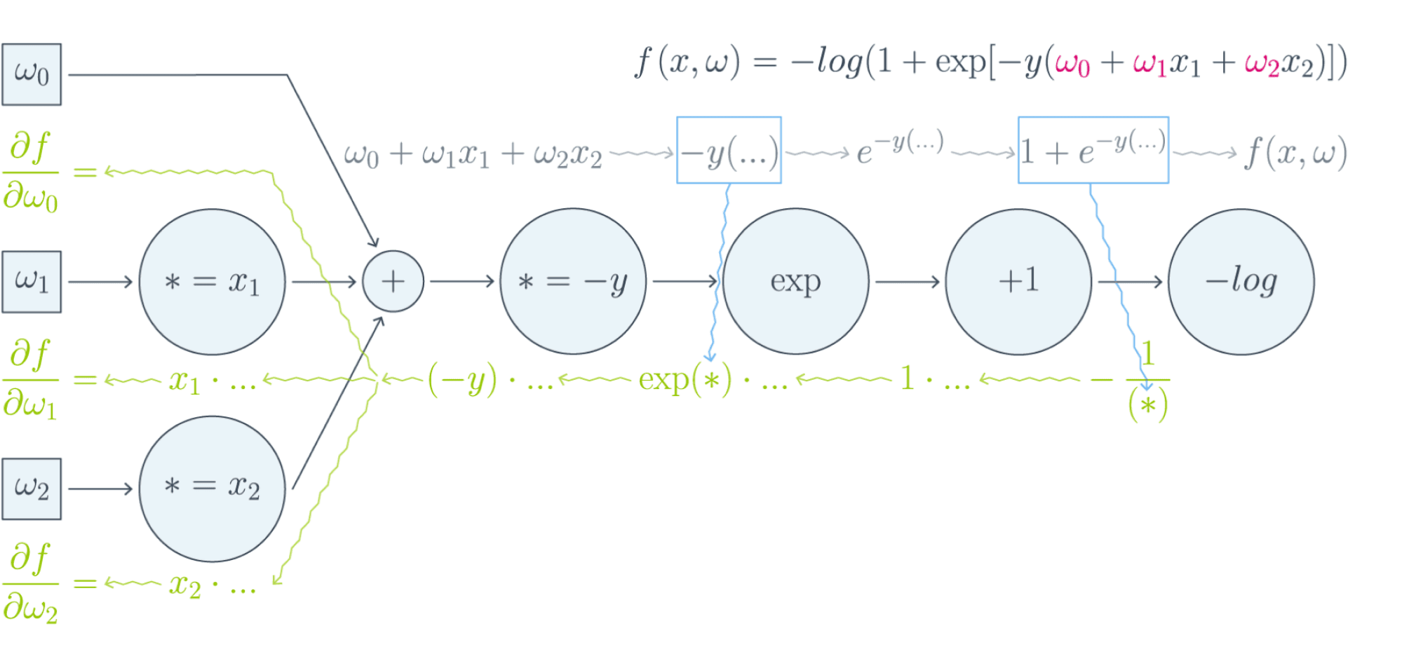
Собирая все множители вместе, получаем:
$$frac{partial f}{partial w_0} = (-y)cdot e^{-y(w_0 + w_1x_1 + w_2x_2)}cdotfrac{-1}{1 + e^{-y(w_0 + w_1x_1 + w_2x_2)}}$$
$$frac{partial f}{partial w_1} = x_1cdot(-y)cdot e^{-y(w_0 + w_1x_1 + w_2x_2)}cdotfrac{-1}{1 + e^{-y(w_0 + w_1x_1 + w_2x_2)}}$$
$$frac{partial f}{partial w_2} = x_2cdot(-y)cdot e^{-y(w_0 + w_1x_1 + w_2x_2)}cdotfrac{-1}{1 + e^{-y(w_0 + w_1x_1 + w_2x_2)}}$$
Таким образом, мы видим, что сперва совершается forward pass для вычисления всех промежуточных значений (и да, все промежуточные представления нужно будет хранить в памяти), а потом запускается backward pass, на котором в один проход вычисляются все градиенты.
Почему же нельзя просто пойти и начать везде вычислять производные?
В главе, посвящённой матричным дифференцированиям, мы поднимаем вопрос о том, что вычислять частные производные по отдельности — это зло, лучше пользоваться матричными вычислениями. Но есть и ещё одна причина: даже и с матричной производной в принципе не всегда хочется иметь дело. Рассмотрим простой пример. Допустим, что $X^r$ и $X^{r+1}$ — два последовательных промежуточных представления $Ntimes M$ и $Ntimes K$, связанных функцией $X^{r+1} = f^{r+1}(X^r)$. Предположим, что мы как-то посчитали производную $frac{partialmathcal{L}}{partial X^{r+1}_{ij}}$ функции потерь $mathcal{L}$, тогда
$$frac{partialmathcal{L}}{partial X^{r}_{st}} = sum_{i,j}frac{partial f^{r+1}_{ij}}{partial X^{r}_{st}}frac{partialmathcal{L}}{partial X^{r+1}_{ij}}$$
И мы видим, что, хотя оба градиента $frac{partialmathcal{L}}{partial X_{ij}^{r+1}}$ и $frac{partialmathcal{L}}{partial X_{st}^{r}}$ являются просто матрицами, в ходе вычислений возникает «четырёхмерный кубик» $frac{partial f_{ij}^{r+1}}{partial X_{st}^{r}}$, даже хранить который весьма болезненно: уж больно много памяти он требует ($N^2MK$ по сравнению с безобидными $NM + NK$, требуемыми для хранения градиентов). Поэтому хочется промежуточные производные $frac{partial f^{r+1}}{partial X^{r}}$ рассматривать не как вычисляемые объекты $frac{partial f_{ij}^{r+1}}{partial X_{st}^{r}}$, а как преобразования, которые превращают $frac{partialmathcal{L}}{partial X_{ij}^{r+1}}$ в $frac{partialmathcal{L}}{partial X_{st}^{r}}$. Целью следующих глав будет именно это: понять, как преобразуется градиент в ходе error backpropagation при переходе через тот или иной слой.
Вы спросите себя: надо ли мне сейчас пойти и прочитать главу учебника про матричное дифференцирование?
Встречный вопрос. Найдите производную функции по вектору $x$:
$$f(x) = x^TAx, Ain Mat_{n}{mathbb{R}}text{ — матрица размера }ntimes n$$
А как всё поменяется, если $A$ тоже зависит от $x$? Чему равен градиент функции, если $A$ является скаляром? Если вы готовы прямо сейчас взять ручку и бумагу и посчитать всё, то вам, вероятно, не надо читать про матричные дифференцирования. Но мы советуем всё-таки заглянуть в эту главу, если обозначения, которые мы будем дальше использовать, покажутся вам непонятными: единой нотации для матричных дифференцирований человечество пока, увы, не изобрело, и переводить с одной на другую не всегда легко.
Мы же сразу перейдём к интересующей нас вещи: к вычислению градиентов сложных функций.
Градиент сложной функции
Напомним, что формула производной сложной функции выглядит следующим образом:
$$left[D_{x_0} (color{#5002A7}{u} circ color{#4CB9C0}{v}) right](h) = color{#5002A7}{left[D_{v(x_0)} u right]} left( color{#4CB9C0}{left[D_{x_0} vright]} (h)right)$$
Теперь разберёмся с градиентами. Пусть $f(x) = g(h(x))$ – скалярная функция. Тогда
$$left[D_{x_0} f right] (x-x_0) = langlenabla_{x_0} f, x-x_0rangle.$$
С другой стороны,
$$left[D_{h(x_0)} g right] left(left[D_{x_0}h right] (x-x_0)right) = langlenabla_{h_{x_0}} g, left[D_{x_0} hright] (x-x_0)rangle = langleleft[D_{x_0} hright]^* nabla_{h(x_0)} g, x-x_0rangle.$$
То есть $color{#FFC100}{nabla_{x_0} f} = color{#348FEA}{left[D_{x_0} h right]}^* color{#FFC100}{nabla_{h(x_0)}}g$ — применение сопряжённого к $D_{x_0} h$ линейного отображения к вектору $nabla_{h(x_0)} g$.
Эта формула — сердце механизма обратного распространения ошибки. Она говорит следующее: если мы каким-то образом получили градиент функции потерь по переменным из некоторого промежуточного представления $X^k$ нейронной сети и при этом знаем, как преобразуется градиент при проходе через слой $f^k$ между $X^{k-1}$ и $X^k$ (то есть как выглядит сопряжённое к дифференциалу слоя между ними отображение), то мы сразу же находим градиент и по переменным из $X^{k-1}$:
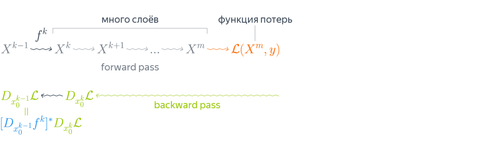
Таким образом слой за слоем мы посчитаем градиенты по всем $X^i$ вплоть до самых первых слоёв.
Далее мы разберёмся, как именно преобразуются градиенты при переходе через некоторые распространённые слои.
Градиенты для типичных слоёв
Рассмотрим несколько важных примеров.
Примеры
-
$f(x) = u(v(x))$, где $x$ — вектор, а $v(x)$ – поэлементное применение $v$:
$$vbegin{pmatrix}
x_1
vdots
x_N
end{pmatrix}
= begin{pmatrix}
v(x_1)
vdots
v(x_N)
end{pmatrix}$$Тогда, как мы знаем,
$$left[D_{x_0} fright] (h) = langlenabla_{x_0} f, hrangle = left[nabla_{x_0} fright]^T h.$$
Следовательно,
$$begin{multline*}
left[D_{v(x_0)} uright] left( left[ D_{x_0} vright] (h)right) = left[nabla_{v(x_0)} uright]^T left(v'(x_0) odot hright) =\[0.1cm]
= sumlimits_i left[nabla_{v(x_0)} uright]_i v'(x_{0i})h_i
= langleleft[nabla_{v(x_0)} uright] odot v'(x_0), hrangle.
end{multline*},$$где $odot$ означает поэлементное перемножение. Окончательно получаем
$$color{#348FEA}{nabla_{x_0} f = left[nabla_{v(x_0)}uright] odot v'(x_0) = v'(x_0) odot left[nabla_{v(x_0)} uright]}$$
Отметим, что если $x$ и $h(x)$ — это просто векторы, то мы могли бы вычислять всё и по формуле $frac{partial f}{partial x_i} = sum_jbig(frac{partial z_j}{partial x_i}big)cdotbig(frac{partial h}{partial z_j}big)$. В этом случае матрица $big(frac{partial z_j}{partial x_i}big)$ была бы диагональной (так как $z_j$ зависит только от $x_j$: ведь $h$ берётся поэлементно), и матричное умножение приводило бы к тому же результату. Однако если $x$ и $h(x)$ — матрицы, то $big(frac{partial z_j}{partial x_i}big)$ представлялась бы уже «четырёхмерным кубиком», и работать с ним было бы ужасно неудобно.
-
$f(X) = g(XW)$, где $X$ и $W$ — матрицы. Как мы знаем,
$$left[D_{X_0} f right] (X-X_0) = text{tr}, left(left[nabla_{X_0} fright]^T (X-X_0)right).$$
Тогда
$$begin{multline*}
left[ D_{X_0W} g right] left(left[D_{X_0} left( ast Wright)right] (H)right) =
left[ D_{X_0W} g right] left(HWright)=\
= text{tr}, left( left[nabla_{X_0W} g right]^T cdot (H) W right) =\
=
text{tr} , left(W left[nabla_{X_0W} (g) right]^T cdot (H)right) = text{tr} , left( left[left[nabla_{X_0W} gright] W^Tright]^T (H)right)
end{multline*}$$Здесь через $ast W$ мы обозначили отображение $Y hookrightarrow YW$, а в предпоследнем переходе использовалось следующее свойство следа:
$$
text{tr} , (A B C) = text{tr} , (C A B),
$$где $A, B, C$ — произвольные матрицы подходящих размеров (то есть допускающие перемножение в обоих приведённых порядках). Следовательно, получаем
$$color{#348FEA}{nabla_{X_0} f = left[nabla_{X_0W} (g) right] cdot W^T}$$
-
$f(W) = g(XW)$, где $W$ и $X$ — матрицы. Для приращения $H = W — W_0$ имеем
$$
left[D_{W_0} f right] (H) = text{tr} , left( left[nabla_{W_0} f right]^T (H)right)
$$Тогда
$$ begin{multline*}
left[D_{XW_0} g right] left( left[D_{W_0} left(X astright) right] (H)right) = left[D_{XW_0} g right] left( XH right) =
= text{tr} , left( left[nabla_{XW_0} g right]^T cdot X (H)right) =
text{tr}, left(left[X^T left[nabla_{XW_0} g right] right]^T (H)right)
end{multline*} $$Здесь через $X ast$ обозначено отображение $Y hookrightarrow XY$. Значит,
$$color{#348FEA}{nabla_{X_0} f = X^T cdot left[nabla_{XW_0} (g)right]}$$
-
$f(X) = g(softmax(X))$, где $X$ — матрица $Ntimes K$, а $softmax$ — функция, которая вычисляется построчно, причём для каждой строки $x$
$$softmax(x) = left(frac{e^{x_1}}{sum_te^{x_t}},ldots,frac{e^{x_K}}{sum_te^{x_t}}right)$$
В этом примере нам будет удобно воспользоваться формализмом с частными производными. Сначала вычислим $frac{partial s_l}{partial x_j}$ для одной строки $x$, где через $s_l$ мы для краткости обозначим $softmax(x)_l = frac{e^{x_l}} {sum_te^{x_t}}$. Нетрудно проверить, что
$$frac{partial s_l}{partial x_j} = begin{cases}
s_j(1 — s_j), & j = l,
-s_ls_j, & jne l
end{cases}$$Так как softmax вычисляется независимо от каждой строчки, то
$$frac{partial s_{rl}}{partial x_{ij}} = begin{cases}
s_{ij}(1 — s_{ij}), & r=i, j = l,
-s_{il}s_{ij}, & r = i, jne l,
0, & rne i
end{cases},$$где через $s_{rl}$ мы обозначили для краткости $softmax(X)_{rl}$.
Теперь пусть $nabla_{rl} = nabla g = frac{partialmathcal{L}}{partial s_{rl}}$ (пришедший со следующего слоя, уже известный градиент). Тогда
$$frac{partialmathcal{L}}{partial x_{ij}} = sum_{r,l}frac{partial s_{rl}}{partial x_{ij}} nabla_{rl}$$
Так как $frac{partial s_{rl}}{partial x_{ij}} = 0$ при $rne i$, мы можем убрать суммирование по $r$:
$$ldots = sum_{l}frac{partial s_{il}}{partial x_{ij}} nabla_{il} = -s_{i1}s_{ij}nabla_{i1} — ldots + s_{ij}(1 — s_{ij})nabla_{ij}-ldots — s_{iK}s_{ij}nabla_{iK} =$$
$$= -s_{ij}sum_t s_{it}nabla_{it} + s_{ij}nabla_{ij}$$
Таким образом, если мы хотим продифференцировать $f$ в какой-то конкретной точке $X_0$, то, смешивая математические обозначения с нотацией Python, мы можем записать:
$$begin{multline*}
color{#348FEA}{nabla_{X_0}f =}\
color{#348FEA}{= -softmax(X_0) odot text{sum}left(
softmax(X_0)odotnabla_{softmax(X_0)}g, text{ axis = 1}
right) +}\
color{#348FEA}{softmax(X_0)odot nabla_{softmax(X_0)}g}
end{multline*}
$$
Backpropagation в общем виде
Подытожим предыдущее обсуждение, описав алгоритм error backpropagation (алгоритм обратного распространения ошибки). Допустим, у нас есть текущие значения весов $W^i_0$ и мы хотим совершить шаг SGD по мини-батчу $X$. Мы должны сделать следующее:
- Совершить forward pass, вычислив и запомнив все промежуточные представления $X = X^0, X^1, ldots, X^m = widehat{y}$.
- Вычислить все градиенты с помощью backward pass.
- С помощью полученных градиентов совершить шаг SGD.
Проиллюстрируем алгоритм на примере двуслойной нейронной сети со скалярным output’ом. Для простоты опустим свободные члены в линейных слоях.
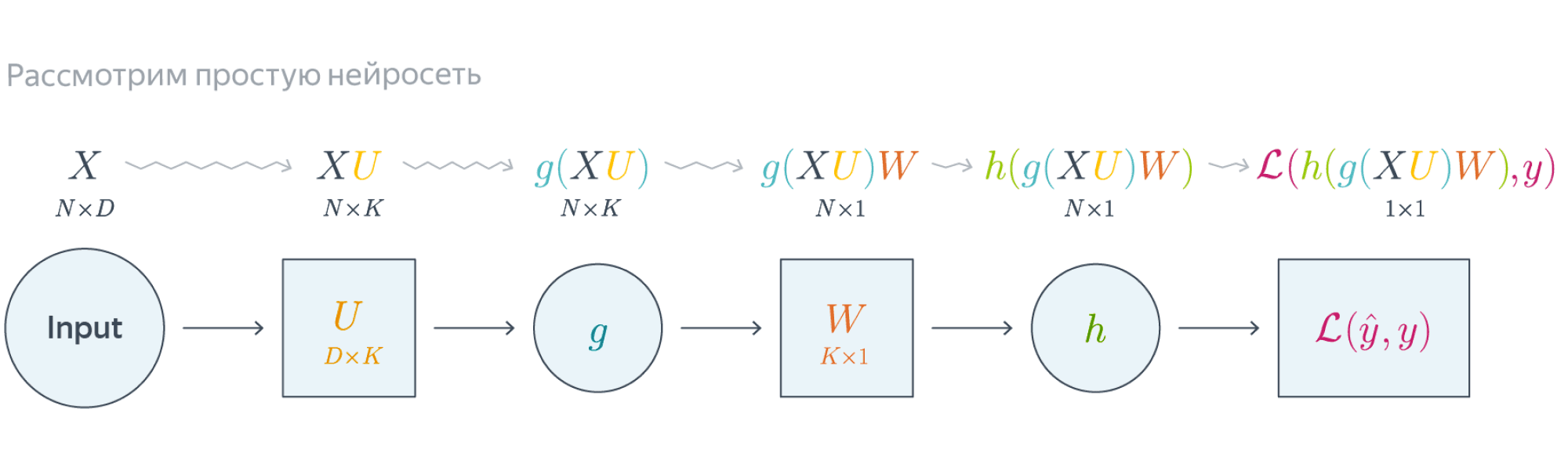 Обучаемые параметры – матрицы $U$ и $W$. Как найти градиенты по ним в точке $U_0, W_0$?
$$nabla_{W_0}mathcal{L} = nabla_{W_0}{left({vphantom{frac12}mathcal{L}circ hcircleft[Wmapsto g(XU_0)Wright]}right)}=$$
$$=g(XU_0)^Tnabla_{g(XU_0)W_0}(mathcal{L}circ h) = underbrace{g(XU_0)^T}_{ktimes N}cdot
left[vphantom{frac12}underbrace{h’left(vphantom{int_0^1}g(XU_0)W_0right)}_{Ntimes 1}odot
underbrace{nabla_{hleft(vphantom{int_0^1}g(XU_0)W_0right)}mathcal{L}}_{Ntimes 1}right]$$
Итого матрица $ktimes 1$, как и $W_0$
$$nabla_{U_0}mathcal{L} = nabla_{U_0}left(vphantom{frac12}
mathcal{L}circ hcircleft[Ymapsto YW_0right]circ gcircleft[ Umapsto XUright]
right)=$$
$$=X^Tcdotnabla_{XU^0}left(vphantom{frac12}mathcal{L}circ hcirc [Ymapsto YW_0]circ gright) =$$
$$=X^Tcdotleft(vphantom{frac12}g'(XU_0)odot
nabla_{g(XU_0)}left[vphantom{in_0^1}mathcal{L}circ hcirc[Ymapsto YW_0right]
right)$$
$$=ldots = underset{Dtimes N}{X^T}cdotleft(vphantom{frac12}
underbrace{g'(XU_0)}_{Ntimes K}odot
underbrace{left[vphantom{int_0^1}left(
underbrace{h’left(vphantom{int_0^1}g(XU_0)W_0right)}_{Ntimes1}odotunderbrace{nabla_{h(vphantom{int_0^1}gleft(XU_0right)W_0)}mathcal{L}}_{Ntimes 1}
right)cdot underbrace{W^T}_{1times K}right]}_{Ntimes K}
right)$$
Итого $Dtimes K$, как и $U_0$
Схематически это можно представить следующим образом:
Backpropagation для двуслойной нейронной сети
Если вы не уследили за вычислениями в предыдущем примере, давайте более подробно разберём его чуть более конкретную версию (для $g = h = sigma$)Рассмотрим двуслойную нейронную сеть для классификации. Мы уже встречали ее ранее при рассмотрении линейно неразделимой выборки. Предсказания получаются следующим образом:
$$
widehat{y} = sigma(X^1 W^2) = sigmaBig(big(sigma(X^0 W^1 )big) W^2 Big).
$$
Пусть $W^1_0$ и $W^2_0$ — текущее приближение матриц весов. Мы хотим совершить шаг по градиенту функции потерь, и для этого мы должны вычислить её градиенты по $W^1$ и $W^2$ в точке $(W^1_0, W^2_0)$.
Прежде всего мы совершаем forward pass, в ходе которого мы должны запомнить все промежуточные представления: $X^1 = X^0 W^1_0$, $X^2 = sigma(X^0 W^1_0)$, $X^3 = sigma(X^0 W^1_0) W^2_0$, $X^4 = sigma(sigma(X^0 W^1_0) W^2_0) = widehat{y}$. Они понадобятся нам дальше.
Для полученных предсказаний вычисляется значение функции потерь:
$$
l = mathcal{L}(y, widehat{y}) = y log(widehat{y}) + (1-y) log(1-widehat{y}).
$$
Дальше мы шаг за шагом будем находить производные по переменным из всё более глубоких слоёв.
-
Градиент $mathcal{L}$ по предсказаниям имеет вид
$$
nabla_{widehat{y}}l = frac{y}{widehat{y}} — frac{1 — y}{1 — widehat{y}} = frac{y — widehat{y}}{widehat{y} (1 — widehat{y})},
$$где, напомним, $ widehat{y} = sigma(X^3) = sigmaBig(big(sigma(X^0 W^1_0 )big) W^2_0 Big)$ (обратите внимание на то, что $W^1_0$ и $W^2_0$ тут именно те, из которых мы делаем градиентный шаг).
-
Следующий слой — поэлементное взятие $sigma$. Как мы помним, при переходе через него градиент поэлементно умножается на производную $sigma$, в которую подставлено предыдущее промежуточное представление:
$$
nabla_{X^3}l = sigma'(X^3)odotnabla_{widehat{y}}l = sigma(X^3)left( 1 — sigma(X^3) right) odot frac{y — widehat{y}}{widehat{y} (1 — widehat{y})} =
$$$$
= sigma(X^3)left( 1 — sigma(X^3) right) odot frac{y — sigma(X^3)}{sigma(X^3) (1 — sigma(X^3))} =
y — sigma(X^3)
$$ -
Следующий слой — умножение на $W^2_0$. В этот момент мы найдём градиент как по $W^2$, так и по $X^2$. При переходе через умножение на матрицу градиент, как мы помним, умножается с той же стороны на транспонированную матрицу, а значит:
$$
color{blue}{nabla_{W^2_0}l} = (X^2)^Tcdot nabla_{X^3}l = (X^2)^Tcdot(y — sigma(X^3)) =
$$$$
= color{blue}{left( sigma(X^0W^1_0) right)^T cdot (y — sigma(sigma(X^0W^1_0)W^2_0))}
$$Аналогичным образом
$$
nabla_{X^2}l = nabla_{X^3}lcdot (W^2_0)^T = (y — sigma(X^3))cdot (W^2_0)^T =
$$$$
= (y — sigma(X^2W_0^2))cdot (W^2_0)^T
$$ -
Следующий слой — снова взятие $sigma$.
$$
nabla_{X^1}l = sigma'(X^1)odotnabla_{X^2}l = sigma(X^1)left( 1 — sigma(X^1) right) odot left( (y — sigma(X^2W_0^2))cdot (W^2_0)^T right) =
$$$$
= sigma(X^1)left( 1 — sigma(X^1) right) odotleft( (y — sigma(sigma(X^1)W_0^2))cdot (W^2_0)^T right)
$$ -
Наконец, последний слой — это умножение $X^0$ на $W^1_0$. Тут мы дифференцируем только по $W^1$:
$$
color{blue}{nabla_{W^1_0}l} = (X^0)^Tcdot nabla_{X^1}l = (X^0)^Tcdot big( sigma(X^1) left( 1 — sigma(X^1) right) odot (y — sigma(sigma(X^1)W_0^2))cdot (W^2_0)^Tbig) =
$$$$
= color{blue}{(X^0)^Tcdotbig(sigma(X^0W^1_0)left( 1 — sigma(X^0W^1_0) right) odot (y — sigma(sigma(X^0W^1_0)W_0^2))cdot (W^2_0)^Tbig) }
$$
Итоговые формулы для градиентов получились страшноватыми, но они были получены друг из друга итеративно с помощью очень простых операций: матричного и поэлементного умножения, в которые порой подставлялись значения заранее вычисленных промежуточных представлений.
Автоматизация и autograd
Итак, чтобы нейросеть обучалась, достаточно для любого слоя $f^k: X^{k-1}mapsto X^k$ с параметрами $W^k$ уметь:
- превращать $nabla_{X^k_0}mathcal{L}$ в $nabla_{X^{k-1}_0}mathcal{L}$ (градиент по выходу в градиент по входу);
- считать градиент по его параметрам $nabla_{W^k_0}mathcal{L}$.
При этом слою совершенно не надо знать, что происходит вокруг. То есть слой действительно может быть запрограммирован как отдельная сущность, умеющая внутри себя делать forward pass и backward pass, после чего слои механически, как кубики в конструкторе, собираются в большую сеть, которая сможет работать как одно целое.
Более того, во многих случаях авторы библиотек для глубинного обучения уже о вас позаботились и создали средства для автоматического дифференцирования выражений (autograd). Поэтому, программируя нейросеть, вы почти всегда можете думать только о forward-проходе, прямом преобразовании данных, предоставив библиотеке дифференцировать всё самостоятельно. Это делает код нейросетей весьма понятным и выразительным (да, в реальности он тоже бывает большим и страшным, но сравните на досуге код какой-нибудь разухабистой нейросети и код градиентного бустинга на решающих деревьях и почувствуйте разницу).
Но это лишь начало
Метод обратного распространения ошибки позволяет удобно посчитать градиенты, но дальше с ними что-то надо делать, и старый добрый SGD едва ли справится с обучением современной сетки. Так что же делать? О некоторых приёмах мы расскажем в следующей главе.
This article is a comprehensive guide to the backpropagation algorithm, the most widely used algorithm for training artificial neural networks. We’ll start by defining forward and backward passes in the process of training neural networks, and then we’ll focus on how backpropagation works in the backward pass. We’ll work on detailed mathematical calculations of the backpropagation algorithm.
Also, we’ll discuss how to implement a backpropagation neural network in Python from scratch using NumPy, based on this GitHub project. The project builds a generic backpropagation neural network that can work with any architecture.
Let’s get started.
Quick overview of Neural Network architecture
In the simplest scenario, the architecture of a neural network consists of some sequential layers, where the layer numbered i is connected to the layer numbered i+1. The layers can be classified into 3 classes:
- Input
- Hidden
- Output
The next figure shows an example of a fully-connected artificial neural network (FCANN), the simplest type of network for demonstrating how the backpropagation algorithm works. The network has an input layer, 2 hidden layers, and an output layer. In the figure, the network architecture is presented horizontally so that each layer is represented vertically from left to right.
Each layer consists of 1 or more neurons represented by circles. Because the network type is fully-connected, then each neuron in layer i is connected with all neurons in layer i+1. If 2 subsequent layers have X and Y neurons, then the number of in-between connections is X*Y.
For each connection, there is an associated weight. The weight is a floating-point number that measures the importance of the connection between 2 neurons. The higher the weight, the more important the connection. The weights are the learnable parameter by which the network makes a prediction. If the weights are good, then the network makes accurate predictions with less error. Otherwise, the weight should be updated to reduce the error.
Assume that a neuron N1 at layer 1 is connected to another neuron N2 at layer 2. Assume also that the value of N2 is calculated according to the next linear equation.
N2=w1N1+b
If N1=4, w1=0.5 (the weight) and b=1 (the bias), then the value of N2 is 3.
N2=0.54+1=2+1=3
This is how a single weight connects 2 neurons together. Note that the input layer has no learnable parameters at all.
Each neuron at layer i+1 has a weight for each connected neuron at layer i , but it only has a single bias. So, if layer i has 10 neurons and layer i+1 has 6 neurons, then the total number of parameters for layer i+1 is:
number of weights+number of biases=10×6 +6=66
The input layer is the first layer in the network, it’s directly connected by the network’s inputs. There can only be a single input layer in the network. For example, if the inputs are student scores in a semester, then these grades are connected to the input layer. In our figure, the input layer has 10 neurons (e.g. scores for 10 courses — a hero student took 10 courses/semester).
The output layer is the last layer which returns the network’s predicted output. Like the input layer, there can only be a single output layer. If the objective of the network is to predict student scores in the next semester, then the output layer should return a score. The architecture in the next figure has a single neuron that returns the next semester’s predicted score.
Between the input and output layers, there might be 0 or more hidden layers. In this example, there are 2 hidden layers with 6 and 4 neurons, respectively. Note that the last hidden layer is connected to the output layer.
Usually, each neuron in the hidden layer uses an activation function like sigmoid or rectified linear unit (ReLU). This helps to capture the non-linear relationship between the inputs and their outputs. The neurons in the output layer also use activation functions like sigmoid (for regression) or SoftMax (for classification).
After building the network architecture, it’s time to start training it with data.
Forward and backward passes in Neural Networks
To train a neural network, there are 2 passes (phases):
- Forward
- Backward
In the forward pass, we start by propagating the data inputs to the input layer, go through the hidden layer(s), measure the network’s predictions from the output layer, and finally calculate the network error based on the predictions the network made.
This network error measures how far the network is from making the correct prediction. For example, if the correct output is 4 and the network’s prediction is 1.3, then the absolute error of the network is 4-1.3=2.7. Note that the process of propagating the inputs from the input layer to the output layer is called forward propagation. Once the network error is calculated, then the forward propagation phase has ended, and backward pass starts.
The next figure shows a red arrow pointing in the direction of the forward propagation.
In the backward pass, the flow is reversed so that we start by propagating the error to the output layer until reaching the input layer passing through the hidden layer(s). The process of propagating the network error from the output layer to the input layer is called backward propagation, or simple backpropagation. The backpropagation algorithm is the set of steps used to update network weights to reduce the network error.
In the next figure, the blue arrow points in the direction of backward propagation.
The forward and backward phases are repeated from some epochs. In each epoch, the following occurs:
- The inputs are propagated from the input to the output layer.
- The network error is calculated.
- The error is propagated from the output layer to the input layer.
We will focus on the backpropagation phase. Let’s discuss the advantages of using the backpropagation algorithm.
Why use the backpropagation algorithm?
Earlier we discussed that the network is trained using 2 passes: forward and backward. At the end of the forward pass, the network error is calculated, and should be as small as possible.
If the current error is high, the network didn’t learn properly from the data. What does this mean? It means that the current set of weights isn’t accurate enough to reduce the network error and make accurate predictions. As a result, we should update network weights to reduce the network error.
The backpropagation algorithm is one of the algorithms responsible for updating network weights with the objective of reducing the network error. It’s quite important.
Here are some of the advantages of the backpropagation algorithm:
- It’s memory-efficient in calculating the derivatives, as it uses less memory compared to other optimization algorithms, like the genetic algorithm. This is a very important feature, especially with large networks.
- The backpropagation algorithm is fast, especially for small and medium-sized networks. As more layers and neurons are added, it starts to get slower as more derivatives are calculated.
- This algorithm is generic enough to work with different network architectures, like convolutional neural networks, generative adversarial networks, fully-connected networks, and more.
- There are no parameters to tune the backpropagation algorithm, so there’s less overhead. The only parameters in the process are related to the gradient descent algorithm, like learning rate.
Next, let’s see how the backpropagation algorithm works, based on a mathematical example.
How backpropagation algorithm works
How the algorithm works is best explained based on a simple network, like the one given in the next figure. It only has an input layer with 2 inputs (X1 and X2), and an output layer with 1 output. There are no hidden layers.
The weights of the inputs are W1 and W2, respectively. The bias is treated as a new input neuron to the output neuron which has a fixed value +1 and a weight b. Both the weights and biases could be referred to as parameters.
Let’s assume that output layer uses the sigmoid activation function defined by the following equation:
![]()
Where s is the sum of products (SOP) between each input and its corresponding weight:
s=X1* W1+ X2*W2+b
To make things simple, a single training sample is used in this example. The next table shows the single training sample with the input and its corresponding desired (i.e. correct) output for the sample. In practice, more training examples are used.
|
X1 |
X2 |
Desired Output |
|
0.1 |
0.3 |
0.03 |
Assume that the initial values for both weights and bias are like in the next table.
For simplicity, the values for all inputs, weights, and bias will be added to the network diagram.
Now, let’s train the network and see how the network will predict the output of the sample based on the current parameters.
As we discussed previously, the training process has 2 phases, forward and backward.
Forward pass
The input of the activation function will be the SOP between each input and its weight. The SOP is then added to the bias to return the output of the neuron:
s=X1* W1+ X2*W2+b
s=0.1* 0.5+ 0.3*0.2+1.83
s=1.94
The value 1.94 is then applied to the activation function (sigmoid), which results in the value 0.874352143.
![]()
![]()
![]()
![]()
![]()
The output of the activation function from the output neuron reflects the predicted output of the sample. It’s obvious that there’s a difference between the desired and expected output. But why? How do we make predicted output closer to desired output? We’ll answer these questions later. For now, let’s see the error of our network based on an error function.
The error functions tell how close the predicted output(s) are from the desired output(s). The optimal value for error is zero, meaning there’s no error at all, and both desired and predicted results are identical. One of the error functions is the squared error function, as defined in the next equation:
Note that the value 12 multiplied by the equation is for simplifying the derivatives calculation using the backpropagation algorithm.
Based on the error function, we can measure the error of our network as follows:
![]()
![]()
![]()
![]()
![]()
The result shows that there is an error, and a large one: (~0.357). The error just gives us an indication of how far the predicted results are from the desired results.
Knowing that there’s an error, what should we do? We should minimize it. To minimize network error, we must change something in the network. Remember that the only parameters we can change are the weights and biases. We can try different weights and biases, and then test our network.
We calculate the error, then the forward pass ends, and we should start the backward pass to calculate the derivatives and update the parameters.
To practically feel the importance of the backpropagation algorithm, let’s try to update the parameters directly without using this algorithm.
Parameters update equation
The parameters can be changed according to the next equation:
W(n+1)=W(n)+η[d(n)-Y(n)]X(n)
Where:
- n: Training step (0, 1, 2, …).
- W(n): Parameters in current training step. Wn=[bn,W1(n),W2(n),W3(n),…, Wm(n)]
- η: Learning rate with a value between 0.0 and 1.0.
- d(n): Desired output.
- Y(n): Predicted output.
- X(n): Current input at which the network made false prediction.
For our network, these parameters have the following values:
- n: 0
- W(n): [1.83, 0.5, 0.2]
- η: Because it is a hyperparameter, then we can choose it 0.01 for example.
- d(n): [0.03].
- Y(n): [0.874352143].
- X(n): [+1, 0.1, 0.3]. First value (+1) is for the bias.
We can update our network parameters as follows:
W(n+1)=W(n)+η[d(n)-Y(n)]X(n)
=[1.83, 0.5, 0.2]+0.01[0.03-0.874352143][+1, 0.1, 0.3]
=[1.83, 0.5, 0.2]+0.01[-0.844352143][+1, 0.1, 0.3]
=[1.83, 0.5, 0.2]+-0.00844352143[+1, 0.1, 0.3]
=[1.83, 0.5, 0.2]+[-0.008443521, -0.000844352, -0.002533056]
=[1.821556479, 0.499155648, 0.197466943]
The new parameters are listed in the next table:
|
W1new |
W2new |
bnew |
|
0.197466943 |
0.499155648 |
1.821556479 |
Based on the new parameters, we will recalculate the predicted output. The new predicted output is used to calculate the new network error. The network parameters are updated according to the calculated error. The process continues to update the parameters and recalculate the predicted output until it reaches an acceptable value for the error.
Here, we successfully updated the parameters without using the backpropagation algorithm. Do we still need that algorithm? Yes. You’ll see why.
The parameters-update equation just depends on the learning rate to update the parameters. It changes all the parameters in a direction opposite to the error.
But, using the backpropagation algorithm, we can know how each single weight correlates with the error. This tells us the effect of each weight on the prediction error. That is, which parameters do we increase, and which ones do we decrease to get the smallest prediction error?
For example, the backpropagation algorithm could tell us useful information, like that increasing the current value of W1 by 1.0 increases the network error by 0.07. This shows us that a smaller value for W1 is better to minimize the error.
Partial derivative
One important operation used in the backward pass is to calculate derivatives. Before getting into the calculations of derivatives in the backward pass, we can start with a simple example to make things easier.
For a multivariate function such as Y=X2Z+H, what’s the effect on the output Y given a change in variable X? We can answer this using partial derivatives, as follows:
![]()
![]()
![]()
Note that everything except X is regarded as a constant. Therefore, H is replaced by 0 after calculating a partial derivative. Here, ∂X means a tiny change of variable X. Similarly, ∂Y means a tiny change of Y. The change of Y is the result of changing X. By making a very small change in X, what’s the effect on Y?
The small change can be an increase or decrease by a tiny value. By substituting the different values of X, we can find how Ychanges with respect to X.
The same procedure can be followed to learn how the NN prediction error changes W.R.T changes in network weights. So, our target is to calculate ∂E/W1 and ∂E/W2 as we have just two weights W1 and W2. Let’s calculate them.
Derivatives of the Prediction Error W.R.T Parameters
Looking at this equation, Y=X2Z+H, it seems straightforward to calculate the partial derivative ∂Y/∂X because there’s an equation relating both Yand X. In our case, there’s no direct equation in which both the prediction error and the weights exist. So, we’re going to use the multivariate chain rule to find the partial derivative of Y W.R.T X.
Prediction Error to Parameters Chain
Let’s try to find the chain relating the prediction error to the weights. The prediction error is calculated based on this equation:
![]()
This equation doesn`t have any parameter. No problem, we can inspect how each term (desired & predicted) of the previous equation is calculated, and substitute with its equation until reaching the parameters.
The desired term in the previous equation is a constant, so there’s no chance for reaching parameters through it. The predicted term is calculated based on the sigmoid function, like in the next equation:
![]()
Again, the equation for calculating the predicted output doesn’t have any parameter. But there’s still variable s (SOP) that already depends on parameters for its calculation, according to this equation:
s=X1* W1+ X2*W2+b
Once we’ve reached an equation that has the parameters (weights and biases), we’ve reached the end of the derivative chain. The next figure presents the chain of derivatives to follow to calculate the derivative of the error W.R.T the parameters.
Note that the derivative of s W.R.T the bias b (∂s/W1) is 0, so it can be omitted. The bias can simply be updated using the learning rate, as we did previously. This leaves us to calculate the derivatives of the 2 weights.
According to the previous figure, to know how prediction error changes W.R.T changes in the parameters we should find the following intermediate derivatives:
- Network error W.R.T the predicted output.
- Predicted output W.R.T the SOP.
- SOP W.R.T each of the 3 parameters.
As a total, there are four intermediate partial derivatives:
∂E/∂Predicted, ∂Predicted/∂s, ∂s/W1 and ∂s/W2
To calculate the derivative of the error W.R.T the weights, simply multiply all the derivatives in the chain from the error to each weight, as in the next 2 equations:
∂E/W1=∂E/∂Predicted* ∂Predicted/∂s* ∂s/W1
∂EW2=∂E/∂Predicted* ∂Predicted/∂s* ∂s/W2
Important note: We used the derivative chain solution because there was no direct equation relating the error and the parameters together. But, we can create an equation relating them and applying partial derivatives directly to it:
E=1/2(desired-1/(1+e-(X1* W1+ X2*W2+b))2
Because this equation seems complex to calculate the derivative of the error W.R.T the parameters directly, it’s preferred to use the multivariate chain rule for simplicity.
Calculating partial derivatives values by substitution
Let’s calculate partial derivatives of each part of the chain we created.
For the derivative of the error W.R.T the predicted output:
∂E/∂Predicted=∂/∂Predicted(1/2(desired-predicted)2)
=2*1/2(desired-predicted)2-1*(0-1)
=(desired-predicted)*(-1)
=predicted-desired
By substituting by the values:
∂E/∂Predicted=predicted-desired=0.874352143-0.03
∂E/∂Predicted=0.844352143
For the derivative of the predicted output W.R.T the SOP:
∂Predicted/∂s=∂/∂s(1/(1+e-s))
Remember: the quotient rule can be used to find the derivative of the sigmoid function as follows:
∂Predicted/∂s=1/(1+e-s)(1-1/(1+e-s))
By substituting by the values:
∂Predicted/∂s=1/(1+e-s)(1-1/(1+e-s))=1/(1+e-1.94)(1-1/(1+e-1.94))
=1/(1+0.143703949)(1-1/(1+0.143703949))
=1/1.143703949(1-1/1.143703949)
=0.874352143(1-0.874352143)
=0.874352143(0.125647857)
∂Predicted/∂s=0.109860473
For the derivative of SOP W.R.T W1:
∂s/W1=∂/∂W1(X1* W1+ X2*W2+b)
=1*X1*(W1)(1-1)+ 0+0
=X1*(W1)(0)
=X1(1)
∂s/W1=X1
By substituting by the values:
∂s/W1=X1=0.1
For the derivative of SOP W.R.T W2:
∂s/W2=∂/∂W2(X1* W1+ X2*W2+b)
=0+1*X2*(W2)(1-1)+0
=X2*(W2)(0)
=X2(1)
∂s/W2=X2
By substituting by the values:
∂s/W2=X2=0.3
After calculating the individual derivatives in all chains, we can multiply all of them to calculate the desired derivatives (i.e. derivative of the error W.R.T each weight).
For the derivative of the error W.R.T W1:
∂E/W1=0.844352143*0.109860473*0.1
∂E/W1=0.009276093
For the derivative of the error W.R.T W2:
∂E/W2=0.844352143*0.109860473*0.3
∂E/W2=0.027828278
Finally, there are two values reflecting how the prediction error changes with respect to the weights:
0.009276093 for W1
0.027828278 for W2
What do these values mean? These results need interpretation.
Interpreting results of backpropagation
There are two useful conclusions from each of the last two derivatives. These conclusions are obtained based on:
- Derivative sign
- Derivative magnitude (DM)
If the derivative sign is positive, that means increasing the weight increases the error. In other words, decreasing the weight decreases the error.
If the derivative sign is negative, increasing the weight decreases the error. In other words, if it’s negative then decreasing the weight increases the error.
But by how much does the error increase or decrease? The derivative magnitude answers this question.
For positive derivatives, increasing the weight by p increases the error by DM*p. For negative derivatives, increasing the weight by p decreases the error by DM*p.
Let’s apply this to our example:
- Because the result of the ∂E/W1 derivative is positive, this means if W1 increases by 1, then the total error increases by 0.009276093.
- Because the result of the ∂E/W2 derivative is positive, this means that if W2 increases by 1 then the total error increases by 0.027828278.
Let’s now update the weights according to the calculated derivatives.
Updating weights
After successfully calculating the derivatives of the error with respect to each individual weight, we can update the weights to improve the prediction. Each weight is updated based on its derivative:
For W1:
W1new=W1-η*∂E/W1
=0.5-0.01*0.009276093
W1new=0.49990723907
For W2:
W2new=W2-η*∂E/W2
=0.2-0.01*0.027828278
W2new= 0.1997217172
Note that the derivative is subtracted (not added) from the old value of the weight, because the derivative is positive.
The new values for the weights are:
- W1=0.49990723907
- W2= 0.1997217172
These 2 weights, in addition to the bias (1.821556479) previously calculated, are used in a new forward pass to calculate the error. It’s expected that the new error will be smaller than the current error (0.356465271).
Here are the new forward pass calculations:
s=X1* W1+ X2*W2+b
s=0.1*0.49990723907+ 0.3*0.1997217172+1.821556479
s=1.931463718067
f(s)=1/(1+e-s)
f(s)=1/(1+e-1.931463718067)
f(s)=0.873411342830056
E=1/2(0.03-0.873411342830056)2
E=0.35567134660719907
When comparing the new error (0.35567134660719907) with the old error (0.356465271), there’s a reduction of 0.0007939243928009043. As long as there’s a reduction, we’re moving in the right direction.
The error reduction is small because we’re using a small learning rate (0.01). To learn about how the learning rate affects the process of training a neural network, read this article.
The forward and backward passes should be repeated until the error is 0 or for a number of epochs (i.e. iterations). This marks the end of the example.
The next section discusses how to implement the backpropagation for the example discussed in this section.
Coding backpropagation in Python
It’s quite easy to implement the backpropagation algorithm for the example discussed in the previous section. In this section, we’ll use this GitHub project to build a network with 2 inputs and 1 output from scratch.
The next code uses NumPy to prepare the inputs (x1=0.1 and x2=0.4), the output with the value 0.7, the learning rate with value 0.01, and assign initial values for the 2 weights w1 and w2. At the end, 2 empty lists are created to hold the network prediction and error in each epoch.
import numpy
x1=0.1
x2=0.4

target = 0.7
learning_rate = 0.01

w1=numpy.random.rand()
w2=numpy.random.rand()

print("Initial W : ", w1, w2)

predicted_output = []
network_error = []
The next code builds some functions that help us in the calculations:
- Sigmoid(): Applies the sigmoid activation function.
- error(): Returns the squared error.
- error_predicted_deriv(): Returns the derivative of the error W.R.T the predicted output.
- sigmoid_sop_deriv(): Returns the derivative of the sigmoid function W.R.T the SOP.
- sop_w_deriv(): Returns the derivative of the SOP W.R.T a single weight.
update_w(): Updates a single weight.
import numpy

def sigmoid(sop):
    return 1.0/(1+numpy.exp(-1*sop))

def error(predicted, target):
    return numpy.power(predicted-target, 2)

def error_predicted_deriv(predicted, target):
    return 2*(predicted-target)

def sigmoid_sop_deriv(sop):
    return sigmoid(sop)*(1.0-sigmoid(sop))

def sop_w_deriv(x):
    return x

def update_w(w, grad, learning_rate):
    return w - learning_rate*grad
Now, we’re ready to do the forward and backward pass calculations for a number of epochs, using a “for” loop according to the next code. The loop goes through 80,000 epochs.
for k in range(80000):

    y = w1*x1 + w2*x2
    predicted = sigmoid(y)
    err = error(predicted, target)

    predicted_output.append(predicted)
    network_error.append(err)


    g1 = error_predicted_deriv(predicted, target)

    g2 = sigmoid_sop_deriv(y)

    g3w1 = sop_w_deriv(x1)
    g3w2 = sop_w_deriv(x2)

    gradw1 = g3w1*g2*g1
    gradw2 = g3w2*g2*g1

    w1 = update_w(w1, gradw1, learning_rate)
    w2 = update_w(w2, gradw2, learning_rate)
In the forward pass, the following lines are executed that calculate the SOP, apply the sigmoid activation function to get the predicted output, and calculate the error. This appends the current network prediction and error in the predicted_output and network_error lists, respectively.
    y = w1*x1 + w2*x2
    predicted = sigmoid(y)
    err = error(predicted, target)

    predicted_output.append(predicted)
    network_error.append(err)
In the backward pass, the remaining lines in the “for” loop are executed to calculate the derivatives in all chains. The derivatives of the error W.R.T to the weights are saved in the variables gradw1 and gradw2. Finally, the weights are updated by calling the update_w() function.
    g1 = error_predicted_deriv(predicted, target)

    g2 = sigmoid_sop_deriv(y)

    g3w1 = sop_w_deriv(x1)
    g3w2 = sop_w_deriv(x2)

    gradw1 = g3w1*g2*g1
    gradw2 = g3w2*g2*g1

    w1 = update_w(w1, gradw1, learning_rate)
    w2 = update_w(w2, gradw2, learning_rate)
The complete code is below. It prints the predicted output after each epoch. Also, it uses the matplotlib library to create 2 plots, showing how the predicted output and the error evolves by epoch.
import numpy
import matplotlib.pyplot

def sigmoid(sop):
    return 1.0/(1+numpy.exp(-1*sop))

def error(predicted, target):
    return numpy.power(predicted-target, 2)

def error_predicted_deriv(predicted, target):
    return 2*(predicted-target)

def sigmoid_sop_deriv(sop):
    return sigmoid(sop)*(1.0-sigmoid(sop))

def sop_w_deriv(x):
    return x

def update_w(w, grad, learning_rate):
    return w - learning_rate*grad

x1=0.1
x2=0.4

target = 0.7
learning_rate = 0.01

w1=numpy.random.rand()
w2=numpy.random.rand()

print("Initial W : ", w1, w2)

predicted_output = []
network_error = []

old_err = 0
for k in range(80000):

    y = w1*x1 + w2*x2
    predicted = sigmoid(y)
    err = error(predicted, target)

    predicted_output.append(predicted)
    network_error.append(err)


    g1 = error_predicted_deriv(predicted, target)

    g2 = sigmoid_sop_deriv(y)

    g3w1 = sop_w_deriv(x1)
    g3w2 = sop_w_deriv(x2)

    gradw1 = g3w1*g2*g1
    gradw2 = g3w2*g2*g1

    w1 = update_w(w1, gradw1, learning_rate)
    w2 = update_w(w2, gradw2, learning_rate)

    print(predicted)

matplotlib.pyplot.figure()
matplotlib.pyplot.plot(network_error)
matplotlib.pyplot.title("Iteration Number vs Error")
matplotlib.pyplot.xlabel("Iteration Number")
matplotlib.pyplot.ylabel("Error")

matplotlib.pyplot.figure()
matplotlib.pyplot.plot(predicted_output)
matplotlib.pyplot.title("Iteration Number vs Prediction")
matplotlib.pyplot.xlabel("Iteration Number")
matplotlib.pyplot.ylabel("Prediction")
In the next figure, the error is plotted for the 80,000 epochs. Note how the error is saturated at the value 3.150953682878443e-13, which is very close to 0.0.
The next figure shows how the predicted output changed by iteration. Remember that the correct output value is set to 0.7 in our example. The output is saturated at the value 0.6999994386664375, very close to 0.7.
The GitHub project also gives a simpler interface to build the network in the Ch09 directory. There’s an example that builds a network with 3 inputs and 1 output. At the end of the code, the function predict() is called to ask the network to predict the output of a new sample [0.2, 3.1, 1.7].
import MLP
import numpy

x = numpy.array([0.1, 0.4, 4.1])
y = numpy.array([0.2])

network_architecture = [7, 5, 4]


trained_ann = MLP.MLP.train(x=x,
                            y=y,
                            net_arch=network_architecture,
                            max_iter=500,
                            learning_rate=0.7,
                            debug=True)

print("Derivative Chains : ", trained_ann["derivative_chain"])
print("Training Time : ", trained_ann["training_time_sec"])
print("Number of Training Iterations : ", trained_ann["elapsed_iter"])

predicted_output = MLP.MLP.predict(trained_ann, numpy.array([0.2, 3.1, 1.7]))
print("Predicted Output : ", predicted_output)
This code uses a module called MLP, a script that builds the backpropagation algorithm while giving the user a simple interface to build, train, and test the network. For details about how to build this script, please refer to this book.
Types of backpropagation
There are 2 main types of the backpropagation algorithm:
- Traditional backpropagation is used for static problems with a fixed input and a fixed output all the time, like predicting the class of an image. In this case, the input image and the output class never change.
- Backpropagation through time (BPTT) targets non-static problems that change over time. It’s applied in time-series models, like recurrent neural networks (RNN).
Drawbacks of the backpropagation algorithm
Even though the backpropagation algorithm is the most widely used algorithm for training neural networks, it has some drawbacks:
- The network should be designed carefully to avoid the vanishing and exploding gradients that affect the way the network learns. For example, the gradients calculated out of the sigmoid activation function may be very small, close to zero, which makes the network unable to update its weights. As a result, no learning happens.
- The backpropagation algorithm considers all neurons in the network equally and calculates their derivatives for each backward pass. Even when dropout layers are used, the derivatives of the dropped neurons are calculated, and then dropped.
- Backpropagation relies on infinitesimal effects (partial derivatives) to perform credit assignment. This could become a serious issue as one considers deeper and more non-linear functions.
- It expects that the error function is convex. For a non-convex function, backpropagation might get stuck in a local optima solution.
- The error function and the activation function must be differentiable in order for the backpropagation algorithm to work. It won’t work with non-differentiable functions.
- In the forward pass, layer i+1 must wait the calculations of layer i to complete. In the backward pass, layer i must wait layer i+1 to complete. This makes all layers of the network locked, waiting for the remainder of the network to execute forwards and propagate error backwards, before they can be updated.
Alternatives to traditional backpropagation
There are a number of alternatives to the traditional back propagation. Below are 4 alternatives.
In Lee, Dong-Hyun, et al. “Difference target propagation.” Joint european conference on machine learning and knowledge discovery in databases. Springer, Cham, 2015., the main idea is to compute targets rather than gradients, at each layer. Like gradients, they are propagated backwards. Target propagation relies on auto-encoders at each layer. Unlike back-propagation, it can be applied even when units exchange stochastic bits rather than real numbers.
For Ma, Wan-Duo Kurt, J. P. Lewis, and W. Bastiaan Kleijn. “The hsic bottleneck: Deep learning without back-propagation.” Proceedings of the AAAI Conference on Artificial Intelligence. Vol. 34. No. 04. 2020., they propose HSIC (Hilbert-Schmidt independence criterion) bottleneck for training deep neural networks. The HSIC bottleneck is an alternative to conventional backpropagation, with a number of distinct advantages. The method facilitates parallel processing, and requires significantly less operations. It doesn’t suffer from exploding or vanishing gradients. It’s biologically more plausible than backpropagation, as there’s no requirement for symmetric feedback.
In Choromanska, Anna, et al. “Beyond backprop: Online alternating minimization with auxiliary variables.” International Conference on Machine Learning. PMLR, 2019., they propose an online (stochastic/mini-batch) alternating minimization (AM) approach for training deep neural networks.
In Jaderberg, Max, et al. “Decoupled neural interfaces using synthetic gradients.” International Conference on Machine Learning. PMLR, 2017., they break the constraint of locking layers by decoupling modules (i.e. layers), and introduce a model of the future computation of the network graph. These models predict what the result of the modelled subgraph will produce using only local information. As a result, the subgraphs can be updated independently and asynchronously.
Conclusion
Hopefully, now you see why backpropagation is the most popular algorithm for training artificial neural networks. It’s quite powerful, and the way it works inside is fascinating. Thanks for reading!
Метод обратного распространения ошибок (англ. backpropagation) — метод вычисления градиента, который используется при обновлении весов в нейронной сети.
Содержание
- 1 Обучение как задача оптимизации
- 2 Дифференцирование для однослойной сети
- 2.1 Находим производную ошибки
- 3 Алгоритм
- 4 Недостатки алгоритма
- 4.1 Паралич сети
- 4.2 Локальные минимумы
- 5 Примечания
- 6 См. также
- 7 Источники информации
Обучение как задача оптимизации
Рассмотрим простую нейронную сеть без скрытых слоев, с двумя входными вершинами и одной выходной, в которых каждый нейрон использует линейную функцию активации, (обычно, многослойные нейронные сети используют нелинейные функции активации, линейные функции используются для упрощения понимания) которая является взвешенной суммой входных данных.
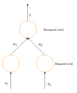
Простая нейронная сеть с двумя входными вершинами и одной выходной
Изначально веса задаются случайно. Затем, нейрон обучается с помощью тренировочного множества, которое в этом случае состоит из множества троек где и — это входные данные сети и — правильный ответ. Начальная сеть, приняв на вход и , вычислит ответ , который вероятно отличается от . Общепринятый метод вычисления несоответствия между ожидаемым и получившимся ответом — квадратичная функция потерь:
- где ошибка.
В качестве примера, обучим сеть на объекте , таким образом, значения и равны 1, а равно 0. Построим график зависимости ошибки от действительного ответа , его результатом будет парабола. Минимум параболы соответствует ответу , минимизирующему . Если тренировочный объект один, минимум касается горизонтальной оси, следовательно ошибка будет нулевая и сеть может выдать ответ равный ожидаемому ответу . Следовательно, задача преобразования входных значений в выходные может быть сведена к задаче оптимизации, заключающейся в поиске функции, которая даст минимальную ошибку.
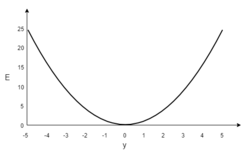
График ошибки для нейрона с линейной функцией активации и одним тренировочным объектом
В таком случае, выходное значение нейрона — взвешенная сумма всех его входных значений:
где и — веса на ребрах, соединяющих входные вершины с выходной. Следовательно, ошибка зависит от весов ребер, входящих в нейрон. И именно это нужно менять в процессе обучения. Распространенный алгоритм для поиска набора весов, минимизирующего ошибку — градиентный спуск. Метод обратного распространения ошибки используется для вычисления самого «крутого» направления для спуска.
Дифференцирование для однослойной сети
Метод градиентного спуска включает в себя вычисление дифференциала квадратичной функции ошибки относительно весов сети. Обычно это делается с помощью метода обратного распространения ошибки. Предположим, что выходной нейрон один, (их может быть несколько, тогда ошибка — это квадратичная норма вектора разницы) тогда квадратичная функция ошибки:
- где — квадратичная ошибка, — требуемый ответ для обучающего образца, — действительный ответ сети.
Множитель добавлен чтобы предотвратить возникновение экспоненты во время дифференцирования. На результат это не повлияет, потому что позже выражение будет умножено на произвольную величину скорости обучения (англ. learning rate).
Для каждого нейрона , его выходное значение определено как
Входные значения нейрона — это взвешенная сумма выходных значений предыдущих нейронов. Если нейрон в первом слое после входного, то входного слоя — это просто входные значения сети. Количество входных значений нейрона . Переменная обозначает вес на ребре между нейроном предыдущего слоя и нейроном текущего слоя.
Функция активации нелинейна и дифференцируема. Одна из распространенных функций активации — сигмоида:
у нее удобная производная:
Находим производную ошибки
Вычисление частной производной ошибки по весам выполняется с помощью цепного правила:
Только одно слагаемое в зависит от , так что
Если нейрон в первом слое после входного, то — это просто .
Производная выходного значения нейрона по его входному значению — это просто частная производная функции активации (предполагается что в качестве функции активации используется сигмоида):
По этой причине данный метод требует дифференцируемой функции активации. (Тем не менее, функция ReLU стала достаточно популярной в последнее время, хоть и не дифференцируема в 0)
Первый множитель легко вычислим, если нейрон находится в выходном слое, ведь в таком случае и
Тем не менее, если произвольный внутренний слой сети, нахождение производной по менее очевидно.
Если рассмотреть как функцию, берущую на вход все нейроны получающие на вход значение нейрона ,
и взять полную производную по , то получим рекурсивное выражение для производной:
Следовательно, производная по может быть вычислена если все производные по выходным значениям следующего слоя известны.
Если собрать все месте:
и
Чтобы обновить вес используя градиентный спуск, нужно выбрать скорость обучения, . Изменение в весах должно отражать влияние на увеличение или уменьшение в . Если , увеличение увеличивает ; наоборот, если , увеличение уменьшает . Новый добавлен к старым весам, и произведение скорости обучения на градиент, умноженный на , гарантирует, что изменения будут всегда уменьшать . Другими словами, в следующем уравнении, всегда изменяет в такую сторону, что уменьшается:
Алгоритм
- — скорость обучения
- — коэффициент инерциальности для сглаживания резких скачков при перемещении по поверхности целевой функции
- — обучающее множество
- — количество повторений
- — функция, подающая x на вход сети и возвращающая выходные значения всех ее узлов
- — количество слоев в сети
- — множество нейронов в слое i
- — множество нейронов в выходном слое
fun BackPropagation:
   init
   repeat :
       for  =  to :
            =
           for :
                =
           for  =  to :
               for :
                    =
           for :
                =
                =
   return
Недостатки алгоритма
Несмотря на многочисленные успешные применения обратного распространения, оно не является универсальным решением. Больше всего неприятностей приносит неопределённо долгий процесс обучения. В сложных задачах для обучения сети могут потребоваться дни или даже недели, она может и вообще не обучиться. Причиной может быть одна из описанных ниже.
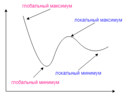
Градиентный спуск может найти локальный минимум вместо глобального
Паралич сети
В процессе обучения сети значения весов могут в результате коррекции стать очень большими величинами. Это может привести к тому, что все или большинство нейронов будут функционировать при очень больших выходных значениях, а производная активирующей функции будет очень мала. Так как посылаемая обратно в процессе обучения ошибка пропорциональна этой производной, то процесс обучения может практически замереть.
Локальные минимумы
Градиентный спуск с обратным распространением ошибок гарантирует нахождение только локального минимума функции; также, возникают проблемы с пересечением плато на поверхности функции ошибки.
Примечания
- Алгоритм обучения многослойной нейронной сети методом обратного распространения ошибки
- Neural Nets
- Understanding backpropagation
См. также
- Нейронные сети, перцептрон
- Стохастический градиентный спуск
- Настройка глубокой сети
- Практики реализации нейронных сетей
Источники информации
- https://en.wikipedia.org/wiki/Backpropagation
- https://ru.wikipedia.org/wiki/Метод_обратного_распространения_ошибки
Backpropagation is an algorithm that backpropagates the errors from the output nodes to the input nodes. Therefore, it is simply referred to as the backward propagation of errors. It uses in the vast applications of neural networks in data mining like Character recognition, Signature verification, etc.
Neural Network:
Neural networks are an information processing paradigm inspired by the human nervous system. Just like in the human nervous system, we have biological neurons in the same way in neural networks we have artificial neurons, artificial neurons are mathematical functions derived from biological neurons. The human brain is estimated to have about 10 billion neurons, each connected to an average of 10,000 other neurons. Each neuron receives a signal through a synapse, which controls the effect of the signconcerning on the neuron.
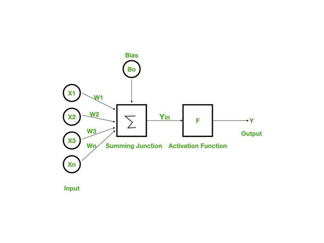
Backpropagation:
Backpropagation is a widely used algorithm for training feedforward neural networks. It computes the gradient of the loss function with respect to the network weights. It is very efficient, rather than naively directly computing the gradient concerning each weight. This efficiency makes it possible to use gradient methods to train multi-layer networks and update weights to minimize loss; variants such as gradient descent or stochastic gradient descent are often used.
The backpropagation algorithm works by computing the gradient of the loss function with respect to each weight via the chain rule, computing the gradient layer by layer, and iterating backward from the last layer to avoid redundant computation of intermediate terms in the chain rule.
Features of Backpropagation:
- it is the gradient descent method as used in the case of simple perceptron network with the differentiable unit.
- it is different from other networks in respect to the process by which the weights are calculated during the learning period of the network.
- training is done in the three stages :
- the feed-forward of input training pattern
- the calculation and backpropagation of the error
- updation of the weight
Working of Backpropagation:
Neural networks use supervised learning to generate output vectors from input vectors that the network operates on. It Compares generated output to the desired output and generates an error report if the result does not match the generated output vector. Then it adjusts the weights according to the bug report to get your desired output.
Backpropagation Algorithm:
Step 1: Inputs X, arrive through the preconnected path.
Step 2: The input is modeled using true weights W. Weights are usually chosen randomly.
Step 3: Calculate the output of each neuron from the input layer to the hidden layer to the output layer.
Step 4: Calculate the error in the outputs
Backpropagation Error= Actual Output – Desired Output
Step 5: From the output layer, go back to the hidden layer to adjust the weights to reduce the error.
Step 6: Repeat the process until the desired output is achieved.

Parameters :
- x = inputs training vector x=(x1,x2,…………xn).
- t = target vector t=(t1,t2……………tn).
- δk = error at output unit.
- δj = error at hidden layer.
- α = learning rate.
- V0j = bias of hidden unit j.
Training Algorithm :
Step 1: Initialize weight to small random values.
Step 2: While the stepsstopping condition is to be false do step 3 to 10.
Step 3: For each training pair do step 4 to 9 (Feed-Forward).
Step 4: Each input unit receives the signal unit and transmitsthe signal xi signal to all the units.
Step 5 : Each hidden unit Zj (z=1 to a) sums its weighted input signal to calculate its net input
zinj = v0j + Σxivij ( i=1 to n)
Applying activation function zj = f(zinj) and sends this signals to all units in the layer about i.e output units
For each output l=unit yk = (k=1 to m) sums its weighted input signals.
yink = w0k + Σ ziwjk (j=1 to a)
and applies its activation function to calculate the output signals.
yk = f(yink)
Backpropagation Error :
Step 6: Each output unit yk (k=1 to n) receives a target pattern corresponding to an input pattern then error is calculated as:
δk = ( tk – yk ) + yink
Step 7: Each hidden unit Zj (j=1 to a) sums its input from all units in the layer above
δinj = Σ δj wjk
The error information term is calculated as :
δj = δinj + zinj
Updation of weight and bias :
Step 8: Each output unit yk (k=1 to m) updates its bias and weight (j=1 to a). The weight correction term is given by :
Δ wjk = α δk zj
and the bias correction term is given by Δwk = α δk.
therefore wjk(new) = wjk(old) + Δ wjk
w0k(new) = wok(old) + Δ wok
for each hidden unit zj (j=1 to a) update its bias and weights (i=0 to n) the weight connection term
Δ vij = α δj xi
and the bias connection on term
Δ v0j = α δj
Therefore vij(new) = vij(old) + Δvij
v0j(new) = v0j(old) + Δv0j
Step 9: Test the stopping condition. The stopping condition can be the minimization of error, number of epochs.
Need for Backpropagation:
Backpropagation is “backpropagation of errors” and is very useful for training neural networks. It’s fast, easy to implement, and simple. Backpropagation does not require any parameters to be set, except the number of inputs. Backpropagation is a flexible method because no prior knowledge of the network is required.
Types of Backpropagation
There are two types of backpropagation networks.
- Static backpropagation: Static backpropagation is a network designed to map static inputs for static outputs. These types of networks are capable of solving static classification problems such as OCR (Optical Character Recognition).
- Recurrent backpropagation: Recursive backpropagation is another network used for fixed-point learning. Activation in recurrent backpropagation is feed-forward until a fixed value is reached. Static backpropagation provides an instant mapping, while recurrent backpropagation does not provide an instant mapping.
Advantages:
- It is simple, fast, and easy to program.
- Only numbers of the input are tuned, not any other parameter.
- It is Flexible and efficient.
- No need for users to learn any special functions.
Disadvantages:
- It is sensitive to noisy data and irregularities. Noisy data can lead to inaccurate results.
- Performance is highly dependent on input data.
- Spending too much time training.
- The matrix-based approach is preferred over a mini-batch.