Block Codes
Takahiro Yamada, in Essentials of Error-Control Coding Techniques, 1990
3.5.2 Product and Concatenated Codes
In order to obtain a code that has high error-correction capability and can be decoded with a relatively simple decoder, we often combine two codes. Product codes and concatenated codes are the most basic methods for combining codes.
A product code is encoded as follows. First, arrange the k1k2 message symbols in a k1 × k2 array and encode each column with an (n1, k1) code C1, as shown in Fig. 3.7A. Then we have an n1 × k2 array. Next, encode each row of this array with an (n2, k2) code C2 (Fig. 3.7B). Thus, we have an n1 × n2 array, which is the codeword of the product code. The resulting product code is an (n1n2, k1k2) code. Let d1 and d2 be the minimum distance of C1 and C2, respectively. Then the minimum distance of the product code is d1d2.

Fig. 3.7. Encoding a product code. (A) Encoding with C1; (B) encoding with C2.
For example, if C1 is an (n1, n1 − 1) parity check code and C2 is an (n2, n2 − 1) parity check code, both with minimum distance 2, the resulting product code is an (n1n2,(n1 − 1)(n2 − 1)) code with minimum distance 4.
A concatenated code (Forney, 1966) is encoded as follows. First, arrange the k1k2 binary message symbols in a k1 × k2 array as in encoding a product code. Then regard each row of this array as an element of GF(2k2), so this array is assumed to be a column vector of length k1, over GF(2k2).
Encode this vector with an (n1, k1) code C1 over GF(2k2) as shown in Fig. 3.8A. Next, we regard the resulting codewords of C1 as an n1 × k2 array over GF(2), and we encode each row with an (n2, k2) code C2 over GF(2) (Fig. 3.8B). The resulting n1 × n2 array is the codeword of the concatenated code, which is an (n1n2, k1k2) code over GF(2). Let d1 and d2 be the minimum distance of C1 and C2, respectively. Then the minimum distance of the concatenated code is d1d2.

Fig. 3.8. Encoding of a concatenated code. (A) Encoding with C1; (B) encoding with C2.
Read full chapter
URL:
https://www.sciencedirect.com/science/article/pii/B9780123707208500076
Quantum Error Correction
Ivan Djordjevic, in Quantum Information Processing and Quantum Error Correction, 2012
7.4.1 Quantum Hamming Bound
The quantum Hamming bound for an [N,K] QECC of error correction capability t is given by
(7.52)∑j=0t(Nj)3j2K≤2N,
where K is the information word length, and N is the codeword length. This inequality is quite straightforward to prove. The number of information words can be found as 2K, the number of error locations is N chooses j, and the number of possible errors {X,Y,Z} at every location is 3j. The total number of errors for all codewords that can be corrected cannot be larger than the code space, which is 2N-dimensional. Analogously to classical codes, the QECCs satisfying the Hamming inequality with equality can be called perfect codes. For t = 1, the quantum Hamming bound becomes (1 + 3N)2K ≤ 2N. For an [N,1] quantum code with t = 1, the quantum Hamming bound is simply 2(1 + 3N) ≤ 2N. The smallest possible N to satisfy the Hamming bound is N = 5, which represents the perfect code. This cyclic code has already been introduced in Section 7.2. It is interesting to note that the quantum Hamming bound is identical to the classical Hamming bound for q-ary linear block codes (LBCs) (see Section 6.7.2) by setting q = 4, corresponding to the cardinality of set of errors {I,X,Y,Z}. This is consistent with the connection we established between QECCs and classical codes over GF(4).
The asymptotic quantum Hamming bound can be obtained by letting N → ∞. For very large N, the last term in summation (7.52) dominates and we can write (Nt)3t2K≤2N. By taking the log2( ) from both sides of the inequality we obtain: log2(Nt)+tlog23+K≤N. By using the approximation log2(Nt)≃NH(t/N), where H(p) is the binary entropy function H(p)=−plogp−(1−p)log(1−p), we obtain the following asymptotic quantum Hamming bound:
(7.53)KN≤1−H(t/N)−tNlog23.
Read full chapter
URL:
https://www.sciencedirect.com/science/article/pii/B9780123854919000071
Turbo-Like Codes Constructions
Sergio Benedetto, … Guido Montorsi, in Academic Press Library in Mobile and Wireless Communications, 2014
5.1 Interleaver theory
Interleavers are devices that permute sequences of symbols: they are widely used for improving error correction capabilities of coding schemes over bursty channels [37]. Their basic theory has received relatively limited attention in the past, apart from some classical papers ([38,39]). Since the introduction of turbo codes [1], where interleavers play a fundamental role, researchers have dedicated many efforts to the interleaver design (e.g., [49]). However, the misunderstanding of the basic interleaver theory often causes confusion in turbo code literature.
In this section, interleaver theory is revisited. The intent is twofold: first, to establish a clear mathematical framework which encompasses old definitions and results on causal interleavers. Second, to extend this theory to noncausal interleavers, which can be useful for turbo codes.
We begin by a proper definition of the key quantities that characterize an interleaver, like its minimum/maximum delay, its characteristic latency, and its period. Then, interleaver equivalence and deinterleavers are carefully studied to derive physically realizable interleavers. Connections between interleaver quantities are then explored, especially those concerning latency, a key parameter for applications. Next, the class of convolutional interleavers is considered and block interleavers, which are the basis of most concatenated code schemes, are introduced as a special case. Finally, we describe the classes of interleavers that have been used in practical and standard turbo codes construction.
Read full chapter
URL:
https://www.sciencedirect.com/science/article/pii/B9780123964991000029
Speech Coding and Channel Coding
Vijay K. Garg, in Wireless Communications & Networking, 2007
8.6.1 Reed-Solomon (RS) Codes
RS coding is a type of FEC. It has been widely used because of its relatively large error correction capability when weighed against its minimal added overhead. RS codes are also easily scaled up or down in error correction capability to match the error rates expected in a given system. It provides a robust error control method for many common types of data transfer mediums, particularly those that are one-way or noisy and sure to produce errors.
In block codes a sequence of K information symbols is encoded in a block of N symbols, N > K, to be transmitted over the channel. For a data source that delivers the information bits at the rate B bps, every T seconds the encoder receives a sequence of K = BT bits which defines a message. After K information bits have entered the encoder, the encoder generates a sequence of coded symbols of length N to be transmitted over the channel. In this transmitted sequence or codeword, N must be greater or equal to K in order to guarantee a unique relationship between each codeword and each of the possible 2K messages. Such a code which maps a block of K information symbols into a block of N coded symbols is called an (N,K) block code. The code rate is r = K/N bits/symbol, N is called the block length.
RS codes are an example of a block coding technique. The data stream to be transmitted is broken up into blocks and redundant data is then added to each block. The size of these blocks and the amount of redundant data added to each block is either specified for a particular application or can be user-defined for a closed system. Within these blocks, the data is further subdivided into a number of symbols, which are generally from 6 to 10 bits in size. The redundant data then consists of additional symbols being added to the end of the transmission. The system-level block diagram for an RS codec is shown in Figure 8.5.

Figure 8.5. RS system level block diagram.
The original data, which is a block consisting of N-R symbols, is run through an RS encoder and R check symbols are added to form a code word of length N. Since RS can be done on any message length and can add any number of check symbols, a particular RS code is expressed as RS (N, N-R) code. N is the total number of symbols per code word; R is the number of check symbols per code word, and N-R is the number of actual information symbols per code word.
RS encoding consists of the generation of check symbols from the original data. The process is based upon finite field arithmetic. The variables to generate a particular RS code include field polynomial and generator polynomial starting roots. The field polynomial is used to determine the order of the elements in the finite field.
Another system-level characteristic of RS coding is whether the implementation is systematic or nonsystematic. A systematic implementation produces a code word that contains the unaltered original input data stream in the first R symbols of the code word. In contrast, in a nonsystematic implementation, the input data stream is altered during the encoding process. Most specifications require systematic coding.
The simplified schematic representation for a systematic RS encoder is shown in Figure 8.6. The input data stream is immediately clocked back out of the function into the check symbol generation circuitry. The fact that the input data stream is clocked out immediately without being altered means that the implementation is systematic. A series of finite fields adds and multiplies results in each register containing one check symbol after the entire input stream has been entered. At that point, the output select is switched over to the check symbol registers, and the check symbols are shifted out at the end of the original message.

Figure 8.6. Systematic RS encoder schematic representation.
The size of the encoder is most heavily affected by the number of check symbols required for the target RS code. The total message length, as well as the field polynomial and first root value, do not have any appreciable effect on the device performance.
A typical RS decode algorithm consists of several major blocks. The first of these blocks is the syndrome calculation, where the incoming symbols are divided into the generator polynomial, which is known from the parameters of the decoder. The check symbols, which form the remainder in the encoder section, will cause the syndrome calculation to be zero in the case of no errors. If there are errors, the resulting polynomial is passed to the Euclid algorithm, where the factors of the remainder are found (see Figure 8.7). The result is evaluated for each of the incoming symbols over many iterations, and any errors are found and corrected. The corrected code word is the output from the decoder. If there are more errors in the code word than can be corrected by the RS code used, then the received code word is output with no changes and a flag is set, stating that the error correction has failed for that code word.

Figure 8.7. RS decoder block diagram.
The error correction capability of a given RS code is a function of the number of check bits appended to the message. In general, it may be assumed that correcting an error requires one check symbol to find the location of the error, and a second check symbol to correct the error. In general then, a given RS code can correct R/2 symbol errors, where R is the number of check symbols in the given RS code. Since RS codes are generally described as an RS (N, N-R) value, the number of errors correctable by this code is [N- (N-R)]/2. This error control capability can be enhanced by use of erasures, a technique that helps to determine the location of an error without using one of the check symbols. An RS implementation supporting erasures would then be able to correct up to R errors.
Since RS codes work on symbols (most commonly equal to one 8-bit byte) as opposed to individual data bits, the number of correctable errors refers to symbol errors. This means that a symbol with all of the bits corrupted is no different than a symbol with only one of its bits corrupted, and error control capability refers to the number of corrupted symbols that can be corrected. RS codes are more suitable to correct consecutive bits. RS codes are generally combined with other coding methods such as Viterbi, which is more suited to correcting evenly distributed errors.
The effective throughput of an RS decoder is a combination of the number of clock cycles required to locate and correct errors after the code word has been received and the speed at which the design can be clocked. Knowing the latency and clock speed allows the user to determine how many symbols per second may be processed by the decoder. In the RS code, there are two RS decoder choices: a high-speed decoder and a low-speed decoder. The trade-off is that the low-speed decoder is usually approximately 20% smaller in device utilization. Note that both decoders operate at the same clock rate, but the low-speed decoder has a longer latency period, resulting in a slower effective symbol rate. As the number of check symbols decreases, the complexity of the decoder decreases, resulting in a smaller design and an increase in performance.
In a real-life RS coding implementation, functions that tend to reside on either side of the RS encoder or decoder are often implemented in programmable logic. One function that often resides after an RS encoder is an interleaver. The task of an interleaver is to scramble the symbols in several RS code words before transmission, effectively spreading any burst error that occurs during transmission over several code words. Spreading this burst error over several code words increases the chance of each code word being able to correct all of its induced errors.
Read full chapter
URL:
https://www.sciencedirect.com/science/article/pii/B9780123735805500429
The Fading Channel Problem and Its Impact on Wireless Communication Systems in Uganda
L.L. Kaluuba, … D. Waigumbulizi, in Proceedings from the International Conference on Advances in Engineering and Technology, 2006
6.1 Adaptive Coding
When a link is experiencing fading, the introduction of additional redundant bits to the information bits to improve error correction capabilities (FEC) allows to maintain the nominal BER while leading to a reduction of the required energy per information bit. Adaptive coding consists in implementing variable coding rate in order to match impairments due to propagation conditions. A gain of varying from 2 to 10 dB can be achieved depending on the coding rate. The limitations of this fade mitigation technique are linked to additional bandwidth requirements for FDMA and larger bursts in the same frame for TDMA. Adaptive coding at constant information data rate then translates in a reduction of the total system throughput when various links are experiencing fading simultaneously.
Read full chapter
URL:
https://www.sciencedirect.com/science/article/pii/B9780080453125500686
Introduction
Hideki Imai, in Essentials of Error-Control Coding Techniques, 1990
1.4.1 Applications to Audio Systems
Since the error rate of devices is high and both random and burst errors occur in digital audio systems, large error-correction capability is required. However, since the correlation between adjacent data is relatively high for audio signals, we can estimate the correct value of erroneous data by using the values of the data before and after the erroneous data. Miscorrection by the decoder causing a click noise must be strictly avoided. Therefore, it is desirable to estimate the correct values of data that are likely to be miscorrected as described previously, instead of correcting any errors at the decoder. Doubly coded Reed—Solomon or cyclic codes with interleaving are often used.
Read full chapter
URL:
https://www.sciencedirect.com/science/article/pii/B9780123707208500052
High-level Design Tools for Complex DSP Applications
Yang Sun, … Tai Ly, in DSP for Embedded and Real-Time Systems, 2012
LDPC decoder design example using PICO
Low-density parity-check (LDPC) codes [6] have received tremendous attention in the coding community because of their excellent error correction capability and near-capacity performance. Some randomly constructed LDPC codes, measured in Bit Error Rate (BER), come very close to the Shannon limit for the AWGN channel with iterative decoding and very long block sizes (on the order of 106 to 107). The remarkable error correction capabilities of LDPC codes have led to their recent adoption in many standards, such as IEEE 802.11n, IEEE 802.16e, and IEEE 802.15.3c.
As wireless standards are rapidly changing and different wireless standards employ different types of LDPC codes, it is very important to design a flexible and scalable LDPC decoder that can be tailored to different wireless applications. In this section, we will explore the design space of efficient implementations of LDPC decoders using the PICO high level synthesis methodology. Under the guidance of the designers, PICO can effectively exploit the parallelism of a given algorithm, and then create an area-time-power efficient hardware architecture for the algorithm. We will present a partial-parallel LDPC decoder implementation using PICO.
A binary LDPC code is a linear block code specified by a very sparse binary M by N parity check matrix:
H·xT = 0,
where x is a codeword and H can be viewed as a bipartite graph where each column and row in H represents a variable node and a check node, respectively. Each element of the parity check matrix is either a zero or a one, where nonzero entries are typically placed at random to achieve good performance. During the encoding process, N-K redundant bits are added to the K information bits to create a codeword length of N bits. The code rate is the ratio of the information bits to the total bits in a codeword. LDPC codes are often represented by a bi-partite graph called a Tanner graph. There are two types of nodes in a Tanner graph, variable nodes and check nodes. A variable node corresponds to a coded bit or a column of the parity check matrix, and a check node corresponds to a parity check equation or a row of the parity check matrix. There is an edge between each pair of nodes if there is a one in the corresponding parity check matrix entry. The number of nonzero elements in each row or column of a parity check matrix is called the degree of that node. An LDPC code is regular or irregular based on the node degrees. If variable or check nodes have different degrees, then the LDPC code is called irregular, otherwise, it is called regular. Generally, irregular codes have better performance than regular codes. On the other hand, irregularity of the code will result in more complex hardware architecture.
Non-zero elements in H are typically placed at random positions to achieve good coding performance. However, this randomness is unfavorable for efficient VLSI implementation that calls for structured design. To address this issue, block-structured quasi-cyclic LDPC codes are recently proposed for several new communication standards such as IEEE 802.11n, IEEE 802.16e, and DVB-S2. As shown in Figure 8-6, the parity check matrix can be viewed as a 2-D array of square sub matrices. Each sub matrix is either a zero matrix or a cyclically shifted identity matrix Ix. Generally, the block-structured parity check matrix H consists of a j-by-k array of z-by-z cyclically shifted identity matrices with random shift values x (0 = < x < = z).

Figure 8-6. A block structured parity check matrix with block rows (or layers) j = 4 and block columns k = 8, where the sub-matrix size is z-by-z.
A good tradeoff between design complexity and decoding throughput is partially parallel decoding by grouping a certain number of variable and check nodes into a cluster for parallel processing. Furthermore, the layered decoding algorithm [7] can be applied to improve the decoding convergence time by a factor of two and hence increases the throughput by two times.
In a block-structured parity-check matrix, which is a j by k array of z by z sub-matrices, each sub-matrix is either a zero or a shifted identity matrix with random shift value. In every layer, each column has at most one 1, which satisfies that there are no data dependencies between the variable node messages, so that the messages flow in tandem only between the adjacent layers. The block size z is variable corresponding to the code definition in the standards.
To simplify the hardware implementation, the scaled min-sum algorithm [8] is used. This algorithm is summarized as follows. Let Qmn denote the variable node log likelihood ratio (LLR) message sent from variable node n to the check node m, Rmn denote the check node LLR message sent from the check node m to the variable node n, and APPn denote the a posteriori probability ratio (APP) for variable node n, then:
Qmn=APPn−RmnRmn′=s×∏j:j≠nsign(Qmj)×(minj:j≠n|Qmj|)APPn′=Qmn+Rmn
where s is a scaling factor. The APP messages are initialized with the channel reliability values of the coded bits.
Hard decisions can be made after every horizontal layer based on the sign of APPn. If all parity-check equations are satisfied or the pre-determined maximum number of iterations is reached, then the decoding algorithm stops. Otherwise, the algorithm repeats for the next horizontal layer.
To implement this algorithm in hardware, we use a block-serial decoding method [9]: data in each layer is processed block-column by block-column. The decoder first reads APP and R messages from memory, calculates Q, and then finds the minimum and the second minimum values for each row m over all column n. Then, the decoder computes the new R and APP values based on the two minimum values, and writes the new R and APP values back to memory. The algorithm is coded in an un-timed C code. A section of the C code is shown in Figure 8-7, which depicts the PPA architecture generated by the PICO C compiler. The parallelism of this architecture is at the level of the sub-matrix size z. Note that the ‘pragma unroll’ statement in the C code will be used by the PICO C compiler to determine the parallelism level. Multiple instances of the decoding cores are generated by the PICO C compiler to achieve a large decoder parallelism.

Figure 8-7. Pipelined LDPC decoder architecture generated by PICO.
As a case study, a flexible LDPC decoder which fully supports the IEEE 802.16e standard was described in an un-timed C procedure, and then the PICO software was used to create synthesizable RTLs. The generated RTLs were synthesized using Synopsys Design Compiler, and placed & routed using Cadence SoC Encounter on a TSMC 65nm 0.9V 8-metal layer CMOS technology. Table 8-1 summarizes the main features of this decoder.
Table 8-1. ASIC synthesis result.
| Core area | 1.2 mm2 |
| Clock frequency | 400 MHz |
| Power consumption | 180 mW |
| Maximum throughput | 415 Mbps |
| Maximum latency | 2.8 μs |
Compared to the manual RTL designs [10, 11] which usually took 6 months to finish, the C based design using PICO technology only took 2 weeks to complete, and is able to achieve high performance in terms of area, power, and throughput. The area overhead is about 15% compared to the manual LDPC decoders [10, 11] that we have implemented before at Rice University.
Read full chapter
URL:
https://www.sciencedirect.com/science/article/pii/B9780123865359000081
Design Technique for an Error-Control Scheme
Tohru Inoue, in Essentials of Error-Control Coding Techniques, 1990
Publisher Summary
This chapter presents design technique for an error-control scheme. To implement actual encoders and decoders for error-correcting codes, it is necessary first to know the specifications required and then to take advantage of the characteristics of the channel. There is a trade-off between error-correction capability and redundancy required, concerning the amount of encoding and decoding hardware, which is also related to the code rate. Errors are classified into two types: (1) random errors and (2) burst errors. In addition to occurring individually, errors can exist as the mixed mode of both types. The chapter describes the method to obtain performance for various important and widely used codes. Cyclic redundancy check is a widely known typical error-detecting code. The decoding procedure for binary Bose, Chaudhuri and Hocquenghem (BCH) codes consists of three steps: (1) calculation of syndromes, (2) calculation of error-locator polynomial using syndromes, and (3) calculation of error locations induced by the error-locator polynomial. BCH decoders, correcting two or three errors, are usually designed to determine the locations of errors directly from the syndrome.
Read full chapter
URL:
https://www.sciencedirect.com/science/article/pii/B978012370720850009X
Video Transmission over Networks
John W. Woods, in Multidimensional Signal, Image, and Video Processing and Coding (Second Edition), 2012
Forward Error Control Coding
The FEC technique is used in many communication systems. In the simplest case, it consists of a block coding wherein a number n − k of parity bits are added to k binary information bits to create a binary channel codeword of length n. The Hamming codes are examples of binary linear codes, where the codewords exist in n-dimensional binary space. Each code is characterized by its minimum Hamming distance dmin, defined as the minimum number of bit differences between two different codewords. Thus, it takes dmin bit errors to change one codeword into another. So the error detection capability of a code is dmin−1, and the error correction capability of a code is ⌊dmin/2⌋, where ⌊⋅⌋ is the least integer function. This last is so because if fewer than ⌊dmin/2⌋ errors occur, the received string is still closer (in Hamming distance) to its error-free version than to any other codeword. Reed-Solomon (RS) codes are also linear, but operate on symbols in a so-called Galois field with 2l elements. Codewords, parity words, and minimal distance are all computed using the arithmetic of this field. An example is l = 4, which corresponds to hexadecimal arithmetic with 16 symbols. The (n, k) = (15,9) RS code has hexadecimal symbols and can correct 3 symbol errors. It codes 9 hexadecimal information symbols (36 bits) into 15 symbol codewords (60 bits) [16]. The RS codes are perfect codes, meaning that the minimum distance between codewords attains the maximum value dmin = n − k + 1 [17]. Thus an (n, k) RS code can detect up to n − k symbol errors. The RS codes are very good for bursts of errors since a short symbol error burst translates into an l times longer binary error burst, when the symbols are written in terms of their l–bit binary code [18]. These RS codes are used in the CD and DVD standards to correct error bursts on decoding.
Read full chapter
URL:
https://www.sciencedirect.com/science/article/pii/B9780123814203000138
Network coding and its applications to satellite systems
Fausto Vieira, Daniel E. Lucani, in Cooperative and Cognitive Satellite Systems, 2015
9.3.5 Overview of broadband multibeam satellites scenarios
In the first scenario, network coding is proposed for providing efficient soft-handover capabilities to terminals over a broadband multibeam satellite networks. The focus is unicast traffic on the forward link. It is assumed that terminals are capable of multibeam reception and that are mounted in high speed platforms such as trains and planes, where handover between (narrow) beams is a common occurrence within the duration of the trip. The network coding gains can be measured in terms of delay gain in recovering from losses, where initial results point to gains up to 70% when comparing with Reed-Solomon codes. Note that this is achieved by exploiting the multipath and FEC capabilities of network coding algorithms, and therefore the algorithms do not employ feedback mechanisms on the return link. Future work would have to focus not only of the optimization of the algorithms for generating the coded packets, but also the cross-layer design required to seamlessly integrate the network coding with the soft-handover management at the lower layers.
In the second scenario, network coding is proposed for broadband multibeam satellite and terminals capable of multibeam reception. The focus is also unicast traffic on the forward link, over multiple beams and the network coding algorithms do not employ feedback mechanisms on the return link. It is assumed that a terminal covered by multiple beams may have different packet loss probabilities per beam. The network coding gains would be in compensating the different packet loss probabilities by providing unequal levels of FEC protection over different beams. Future work would have to analyze if there are efficiencies in not providing the same packet loss probabilities over multiple beams but rather different levels of network coding resilience. Furthermore, the network coding algorithms and the cross-layer design would also need to be explored in detail.
In the third scenario, network coding is proposed for providing beam level load balancing mechanisms for broadband multibeam satellite networks. It is assumed that terminals are capable of multibeam reception and that many are covered by multiple beams. The network coding gains are expected to be around 50% in terms of the aggregate data rates that can be provided over a satellite with a conventional payload with realistic asymmetric demand patterns per beam. Future work would have to focus on the optimization of the network coding algorithms, the cross-layer design for integrating the multibeam reception, the resource allocation mechanisms, and the deployment strategies for terminals with multibeam reception capabilities.
Read full chapter
URL:
https://www.sciencedirect.com/science/article/pii/B9780127999487000098
- error-correcting capability
-
- возможность исправления ошибок
возможность исправления ошибок
исправляющая способность
—
[Л.Г.Суменко. Англо-русский словарь по информационным технологиям. М.: ГП ЦНИИС, 2003.]Тематики
- информационные технологии в целом
Синонимы
- исправляющая способность
EN
- error-correcting capability
Англо-русский словарь нормативно-технической терминологии.
.
2015.
Смотреть что такое «error-correcting capability» в других словарях:
-
Time-Limited Error Recovery — (TLER) is a name used by Western Digital for a hard drive feature that allows improved error handling in a RAID environment. In some cases, there is a conflict whether error handling should be undertaken by the hard drive or by the RAID… … Wikipedia
-
Advanced Audio Coding — AAC redirects here. For other uses, see AAC (disambiguation). Advanced Audio Codings iTunes standard AAC file icon Filename extension .m4a, .m4b, .m4p, .m4v, .m4r, .3gp, .mp4, .aac Internet media type audio/aac, audio/aacp, au … Wikipedia
-
Корректирующая способность — (англ. error correcting capability) характеристика кода , описывающая возможность исправить ошибки в кодовых словах. Определяется как целое число, меньшее половины от минимального расстояния между кодовыми словами минус один в принятой… … Википедия
-
возможность исправления ошибок — исправляющая способность — [Л.Г.Суменко. Англо русский словарь по информационным технологиям. М.: ГП ЦНИИС, 2003.] Тематики информационные технологии в целом Синонимы исправляющая способность EN error correcting capability … Справочник технического переводчика
-
information theory — the mathematical theory concerned with the content, transmission, storage, and retrieval of information, usually in the form of messages or data, and esp. by means of computers. [1945 50] * * * ▪ mathematics Introduction a mathematical… … Universalium
-
Mathematics and Physical Sciences — ▪ 2003 Introduction Mathematics Mathematics in 2002 was marked by two discoveries in number theory. The first may have practical implications; the second satisfied a 150 year old curiosity. Computer scientist Manindra Agrawal of the… … Universalium
-
Abkürzungen/Computer — Dies ist eine Liste technischer Abkürzungen, die im IT Bereich verwendet werden. A [nach oben] AA Antialiasing AAA authentication, authorization and accounting, siehe Triple A System AAC Advanced Audio Coding AACS … Deutsch Wikipedia
-
Liste der Abkürzungen (Computer) — Dies ist eine Liste technischer Abkürzungen, die im IT Bereich verwendet werden. A [nach oben] AA Antialiasing AAA authentication, authorization and accounting, siehe Triple A System AAC Advanced Audio Coding AACS … Deutsch Wikipedia
-
Packet (information technology) — In information technology, a packet is a formatted unit of data carried by a packet mode computer network. Computer communications links that do not support packets, such as traditional point to point telecommunications links, simply transmit… … Wikipedia
-
Network packet — In computer networking, a packet is a formatted unit of data carried by a packet mode computer network. Computer communications links that do not support packets, such as traditional point to point telecommunications links, simply transmit data… … Wikipedia
-
Convolutional code — In telecommunication, a convolutional code is a type of error correcting code in which each m bit information symbol (each m bit string) to be encoded is transformed into an n bit symbol, where m/n is the code rate (n ≥ m) and the transformation… … Wikipedia
«Interleaver» redirects here. For the fiber-optic device, see optical interleaver.
In computing, telecommunication, information theory, and coding theory, forward error correction (FEC) or channel coding[1][2][3] is a technique used for controlling errors in data transmission over unreliable or noisy communication channels.
The central idea is that the sender encodes the message in a redundant way, most often by using an error correction code or error correcting code, (ECC).[4][5] The redundancy allows the receiver not only to detect errors that may occur anywhere in the message, but often to correct a limited number of errors. Therefore a reverse channel to request re-transmission may not be needed. The cost is a fixed, higher forward channel bandwidth.
The American mathematician Richard Hamming pioneered this field in the 1940s and invented the first error-correcting code in 1950: the Hamming (7,4) code.[5]
FEC can be applied in situations where re-transmissions are costly or impossible, such as one-way communication links or when transmitting to multiple receivers in multicast.
Long-latency connections also benefit; in the case of a satellite orbiting Uranus, retransmission due to errors can create a delay of five hours. FEC is widely used in modems and in cellular networks, as well.
FEC processing in a receiver may be applied to a digital bit stream or in the demodulation of a digitally modulated carrier. For the latter, FEC is an integral part of the initial analog-to-digital conversion in the receiver. The Viterbi decoder implements a soft-decision algorithm to demodulate digital data from an analog signal corrupted by noise. Many FEC decoders can also generate a bit-error rate (BER) signal which can be used as feedback to fine-tune the analog receiving electronics.
FEC information is added to mass storage (magnetic, optical and solid state/flash based) devices to enable recovery of corrupted data, and is used as ECC computer memory on systems that require special provisions for reliability.
The maximum proportion of errors or missing bits that can be corrected is determined by the design of the ECC, so different forward error correcting codes are suitable for different conditions. In general, a stronger code induces more redundancy that needs to be transmitted using the available bandwidth, which reduces the effective bit-rate while improving the received effective signal-to-noise ratio. The noisy-channel coding theorem of Claude Shannon can be used to compute the maximum achievable communication bandwidth for a given maximum acceptable error probability. This establishes bounds on the theoretical maximum information transfer rate of a channel with some given base noise level. However, the proof is not constructive, and hence gives no insight of how to build a capacity achieving code. After years of research, some advanced FEC systems like polar code[3] come very close to the theoretical maximum given by the Shannon channel capacity under the hypothesis of an infinite length frame.
How it works[edit]
ECC is accomplished by adding redundancy to the transmitted information using an algorithm. A redundant bit may be a complex function of many original information bits. The original information may or may not appear literally in the encoded output; codes that include the unmodified input in the output are systematic, while those that do not are non-systematic.
A simplistic example of ECC is to transmit each data bit 3 times, which is known as a (3,1) repetition code. Through a noisy channel, a receiver might see 8 versions of the output, see table below.
| Triplet received | Interpreted as |
|---|---|
| 000 | 0 (error-free) |
| 001 | 0 |
| 010 | 0 |
| 100 | 0 |
| 111 | 1 (error-free) |
| 110 | 1 |
| 101 | 1 |
| 011 | 1 |
This allows an error in any one of the three samples to be corrected by «majority vote», or «democratic voting». The correcting ability of this ECC is:
- Up to 1 bit of triplet in error, or
- up to 2 bits of triplet omitted (cases not shown in table).
Though simple to implement and widely used, this triple modular redundancy is a relatively inefficient ECC. Better ECC codes typically examine the last several tens or even the last several hundreds of previously received bits to determine how to decode the current small handful of bits (typically in groups of 2 to 8 bits).
Averaging noise to reduce errors[edit]
ECC could be said to work by «averaging noise»; since each data bit affects many transmitted symbols, the corruption of some symbols by noise usually allows the original user data to be extracted from the other, uncorrupted received symbols that also depend on the same user data.
- Because of this «risk-pooling» effect, digital communication systems that use ECC tend to work well above a certain minimum signal-to-noise ratio and not at all below it.
- This all-or-nothing tendency – the cliff effect – becomes more pronounced as stronger codes are used that more closely approach the theoretical Shannon limit.
- Interleaving ECC coded data can reduce the all or nothing properties of transmitted ECC codes when the channel errors tend to occur in bursts. However, this method has limits; it is best used on narrowband data.
Most telecommunication systems use a fixed channel code designed to tolerate the expected worst-case bit error rate, and then fail to work at all if the bit error rate is ever worse.
However, some systems adapt to the given channel error conditions: some instances of hybrid automatic repeat-request use a fixed ECC method as long as the ECC can handle the error rate, then switch to ARQ when the error rate gets too high;
adaptive modulation and coding uses a variety of ECC rates, adding more error-correction bits per packet when there are higher error rates in the channel, or taking them out when they are not needed.
Types of ECC[edit]

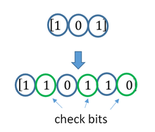
A block code (specifically a Hamming code) where redundant bits are added as a block to the end of the initial message
A continuous code convolutional code where redundant bits are added continuously into the structure of the code word
The two main categories of ECC codes are block codes and convolutional codes.
- Block codes work on fixed-size blocks (packets) of bits or symbols of predetermined size. Practical block codes can generally be hard-decoded in polynomial time to their block length.
- Convolutional codes work on bit or symbol streams of arbitrary length. They are most often soft decoded with the Viterbi algorithm, though other algorithms are sometimes used. Viterbi decoding allows asymptotically optimal decoding efficiency with increasing constraint length of the convolutional code, but at the expense of exponentially increasing complexity. A convolutional code that is terminated is also a ‘block code’ in that it encodes a block of input data, but the block size of a convolutional code is generally arbitrary, while block codes have a fixed size dictated by their algebraic characteristics. Types of termination for convolutional codes include «tail-biting» and «bit-flushing».
There are many types of block codes; Reed–Solomon coding is noteworthy for its widespread use in compact discs, DVDs, and hard disk drives. Other examples of classical block codes include Golay, BCH, Multidimensional parity, and Hamming codes.
Hamming ECC is commonly used to correct NAND flash memory errors.[6]
This provides single-bit error correction and 2-bit error detection.
Hamming codes are only suitable for more reliable single-level cell (SLC) NAND.
Denser multi-level cell (MLC) NAND may use multi-bit correcting ECC such as BCH or Reed–Solomon.[7][8] NOR Flash typically does not use any error correction.[7]
Classical block codes are usually decoded using hard-decision algorithms,[9] which means that for every input and output signal a hard decision is made whether it corresponds to a one or a zero bit. In contrast, convolutional codes are typically decoded using soft-decision algorithms like the Viterbi, MAP or BCJR algorithms, which process (discretized) analog signals, and which allow for much higher error-correction performance than hard-decision decoding.
Nearly all classical block codes apply the algebraic properties of finite fields. Hence classical block codes are often referred to as algebraic codes.
In contrast to classical block codes that often specify an error-detecting or error-correcting ability, many modern block codes such as LDPC codes lack such guarantees. Instead, modern codes are evaluated in terms of their bit error rates.
Most forward error correction codes correct only bit-flips, but not bit-insertions or bit-deletions.
In this setting, the Hamming distance is the appropriate way to measure the bit error rate.
A few forward error correction codes are designed to correct bit-insertions and bit-deletions, such as Marker Codes and Watermark Codes.
The Levenshtein distance is a more appropriate way to measure the bit error rate when using such codes.
[10]
Code-rate and the tradeoff between reliability and data rate[edit]
The fundamental principle of ECC is to add redundant bits in order to help the decoder to find out the true message that was encoded by the transmitter. The code-rate of a given ECC system is defined as the ratio between the number of information bits and the total number of bits (i.e., information plus redundancy bits) in a given communication package. The code-rate is hence a real number. A low code-rate close to zero implies a strong code that uses many redundant bits to achieve a good performance, while a large code-rate close to 1 implies a weak code.
The redundant bits that protect the information have to be transferred using the same communication resources that they are trying to protect. This causes a fundamental tradeoff between reliability and data rate.[11] In one extreme, a strong code (with low code-rate) can induce an important increase in the receiver SNR (signal-to-noise-ratio) decreasing the bit error rate, at the cost of reducing the effective data rate. On the other extreme, not using any ECC (i.e., a code-rate equal to 1) uses the full channel for information transfer purposes, at the cost of leaving the bits without any additional protection.
One interesting question is the following: how efficient in terms of information transfer can an ECC be that has a negligible decoding error rate? This question was answered by Claude Shannon with his second theorem, which says that the channel capacity is the maximum bit rate achievable by any ECC whose error rate tends to zero:[12] His proof relies on Gaussian random coding, which is not suitable to real-world applications. The upper bound given by Shannon’s work inspired a long journey in designing ECCs that can come close to the ultimate performance boundary. Various codes today can attain almost the Shannon limit. However, capacity achieving ECCs are usually extremely complex to implement.
The most popular ECCs have a trade-off between performance and computational complexity. Usually, their parameters give a range of possible code rates, which can be optimized depending on the scenario. Usually, this optimization is done in order to achieve a low decoding error probability while minimizing the impact to the data rate. Another criterion for optimizing the code rate is to balance low error rate and retransmissions number in order to the energy cost of the communication.[13]
Concatenated ECC codes for improved performance[edit]
Classical (algebraic) block codes and convolutional codes are frequently combined in concatenated coding schemes in which a short constraint-length Viterbi-decoded convolutional code does most of the work and a block code (usually Reed–Solomon) with larger symbol size and block length «mops up» any errors made by the convolutional decoder. Single pass decoding with this family of error correction codes can yield very low error rates, but for long range transmission conditions (like deep space) iterative decoding is recommended.
Concatenated codes have been standard practice in satellite and deep space communications since Voyager 2 first used the technique in its 1986 encounter with Uranus. The Galileo craft used iterative concatenated codes to compensate for the very high error rate conditions caused by having a failed antenna.
Low-density parity-check (LDPC)[edit]
Low-density parity-check (LDPC) codes are a class of highly efficient linear block
codes made from many single parity check (SPC) codes. They can provide performance very close to the channel capacity (the theoretical maximum) using an iterated soft-decision decoding approach, at linear time complexity in terms of their block length. Practical implementations rely heavily on decoding the constituent SPC codes in parallel.
LDPC codes were first introduced by Robert G. Gallager in his PhD thesis in 1960,
but due to the computational effort in implementing encoder and decoder and the introduction of Reed–Solomon codes,
they were mostly ignored until the 1990s.
LDPC codes are now used in many recent high-speed communication standards, such as DVB-S2 (Digital Video Broadcasting – Satellite – Second Generation), WiMAX (IEEE 802.16e standard for microwave communications), High-Speed Wireless LAN (IEEE 802.11n),[14] 10GBase-T Ethernet (802.3an) and G.hn/G.9960 (ITU-T Standard for networking over power lines, phone lines and coaxial cable). Other LDPC codes are standardized for wireless communication standards within 3GPP MBMS (see fountain codes).
Turbo codes[edit]
Turbo coding is an iterated soft-decoding scheme that combines two or more relatively simple convolutional codes and an interleaver to produce a block code that can perform to within a fraction of a decibel of the Shannon limit. Predating LDPC codes in terms of practical application, they now provide similar performance.
One of the earliest commercial applications of turbo coding was the CDMA2000 1x (TIA IS-2000) digital cellular technology developed by Qualcomm and sold by Verizon Wireless, Sprint, and other carriers. It is also used for the evolution of CDMA2000 1x specifically for Internet access, 1xEV-DO (TIA IS-856). Like 1x, EV-DO was developed by Qualcomm, and is sold by Verizon Wireless, Sprint, and other carriers (Verizon’s marketing name for 1xEV-DO is Broadband Access, Sprint’s consumer and business marketing names for 1xEV-DO are Power Vision and Mobile Broadband, respectively).
Local decoding and testing of codes[edit]
Sometimes it is only necessary to decode single bits of the message, or to check whether a given signal is a codeword, and do so without looking at the entire signal. This can make sense in a streaming setting, where codewords are too large to be classically decoded fast enough and where only a few bits of the message are of interest for now. Also such codes have become an important tool in computational complexity theory, e.g., for the design of probabilistically checkable proofs.
Locally decodable codes are error-correcting codes for which single bits of the message can be probabilistically recovered by only looking at a small (say constant) number of positions of a codeword, even after the codeword has been corrupted at some constant fraction of positions. Locally testable codes are error-correcting codes for which it can be checked probabilistically whether a signal is close to a codeword by only looking at a small number of positions of the signal.
Interleaving[edit]
«Interleaver» redirects here. For the fiber-optic device, see optical interleaver.

A short illustration of interleaving idea
Interleaving is frequently used in digital communication and storage systems to improve the performance of forward error correcting codes. Many communication channels are not memoryless: errors typically occur in bursts rather than independently. If the number of errors within a code word exceeds the error-correcting code’s capability, it fails to recover the original code word. Interleaving alleviates this problem by shuffling source symbols across several code words, thereby creating a more uniform distribution of errors.[15] Therefore, interleaving is widely used for burst error-correction.
The analysis of modern iterated codes, like turbo codes and LDPC codes, typically assumes an independent distribution of errors.[16] Systems using LDPC codes therefore typically employ additional interleaving across the symbols within a code word.[17]
For turbo codes, an interleaver is an integral component and its proper design is crucial for good performance.[15][18] The iterative decoding algorithm works best when there are not short cycles in the factor graph that represents the decoder; the interleaver is chosen to avoid short cycles.
Interleaver designs include:
- rectangular (or uniform) interleavers (similar to the method using skip factors described above)
- convolutional interleavers
- random interleavers (where the interleaver is a known random permutation)
- S-random interleaver (where the interleaver is a known random permutation with the constraint that no input symbols within distance S appear within a distance of S in the output).[19]
- a contention-free quadratic permutation polynomial (QPP).[20] An example of use is in the 3GPP Long Term Evolution mobile telecommunication standard.[21]
In multi-carrier communication systems, interleaving across carriers may be employed to provide frequency diversity, e.g., to mitigate frequency-selective fading or narrowband interference.[22]
Example[edit]
Transmission without interleaving:
Error-free message:                                 aaaabbbbccccddddeeeeffffgggg
Transmission with a burst error:                    aaaabbbbccc____deeeeffffgggg
Here, each group of the same letter represents a 4-bit one-bit error-correcting codeword. The codeword cccc is altered in one bit and can be corrected, but the codeword dddd is altered in three bits, so either it cannot be decoded at all or it might be decoded incorrectly.
With interleaving:
Error-free code words:                              aaaabbbbccccddddeeeeffffgggg
Interleaved:                                        abcdefgabcdefgabcdefgabcdefg
Transmission with a burst error:                    abcdefgabcd____bcdefgabcdefg
Received code words after deinterleaving:           aa_abbbbccccdddde_eef_ffg_gg
In each of the codewords «aaaa», «eeee», «ffff», and «gggg», only one bit is altered, so one-bit error-correcting code will decode everything correctly.
Transmission without interleaving:
Original transmitted sentence:                      ThisIsAnExampleOfInterleaving
Received sentence with a burst error:               ThisIs______pleOfInterleaving
The term «AnExample» ends up mostly unintelligible and difficult to correct.
With interleaving:
Transmitted sentence:                               ThisIsAnExampleOfInterleaving...
Error-free transmission:                            TIEpfeaghsxlIrv.iAaenli.snmOten.
Received sentence with a burst error:               TIEpfe______Irv.iAaenli.snmOten.
Received sentence after deinterleaving:             T_isI_AnE_amp_eOfInterle_vin_...
No word is completely lost and the missing letters can be recovered with minimal guesswork.
Disadvantages of interleaving[edit]
Use of interleaving techniques increases total delay. This is because the entire interleaved block must be received before the packets can be decoded.[23] Also interleavers hide the structure of errors; without an interleaver, more advanced decoding algorithms can take advantage of the error structure and achieve more reliable communication than a simpler decoder combined with an interleaver[citation needed]. An example of such an algorithm is based on neural network[24] structures.
Software for error-correcting codes[edit]
Simulating the behaviour of error-correcting codes (ECCs) in software is a common practice to design, validate and improve ECCs. The upcoming wireless 5G standard raises a new range of applications for the software ECCs: the Cloud Radio Access Networks (C-RAN) in a Software-defined radio (SDR) context. The idea is to directly use software ECCs in the communications. For instance in the 5G, the software ECCs could be located in the cloud and the antennas connected to this computing resources: improving this way the flexibility of the communication network and eventually increasing the energy efficiency of the system.
In this context, there are various available Open-source software listed below (non exhaustive).
- AFF3CT(A Fast Forward Error Correction Toolbox): a full communication chain in C++ (many supported codes like Turbo, LDPC, Polar codes, etc.), very fast and specialized on channel coding (can be used as a program for simulations or as a library for the SDR).
- IT++: a C++ library of classes and functions for linear algebra, numerical optimization, signal processing, communications, and statistics.
- OpenAir: implementation (in C) of the 3GPP specifications concerning the Evolved Packet Core Networks.
List of error-correcting codes[edit]
| Distance | Code |
|---|---|
| 2 (single-error detecting) | Parity |
| 3 (single-error correcting) | Triple modular redundancy |
| 3 (single-error correcting) | perfect Hamming such as Hamming(7,4) |
| 4 (SECDED) | Extended Hamming |
| 5 (double-error correcting) | |
| 6 (double-error correct-/triple error detect) | Nordstrom-Robinson code |
| 7 (three-error correcting) | perfect binary Golay code |
| 8 (TECFED) | extended binary Golay code |
- AN codes
- BCH code, which can be designed to correct any arbitrary number of errors per code block.
- Barker code used for radar, telemetry, ultra sound, Wifi, DSSS mobile phone networks, GPS etc.
- Berger code
- Constant-weight code
- Convolutional code
- Expander codes
- Group codes
- Golay codes, of which the Binary Golay code is of practical interest
- Goppa code, used in the McEliece cryptosystem
- Hadamard code
- Hagelbarger code
- Hamming code
- Latin square based code for non-white noise (prevalent for example in broadband over powerlines)
- Lexicographic code
- Linear Network Coding, a type of erasure correcting code across networks instead of point-to-point links
- Long code
- Low-density parity-check code, also known as Gallager code, as the archetype for sparse graph codes
- LT code, which is a near-optimal rateless erasure correcting code (Fountain code)
- m of n codes
- Nordstrom-Robinson code, used in Geometry and Group Theory[25]
- Online code, a near-optimal rateless erasure correcting code
- Polar code (coding theory)
- Raptor code, a near-optimal rateless erasure correcting code
- Reed–Solomon error correction
- Reed–Muller code
- Repeat-accumulate code
- Repetition codes, such as Triple modular redundancy
- Spinal code, a rateless, nonlinear code based on pseudo-random hash functions[26]
- Tornado code, a near-optimal erasure correcting code, and the precursor to Fountain codes
- Turbo code
- Walsh–Hadamard code
- Cyclic redundancy checks (CRCs) can correct 1-bit errors for messages at most
 bits long for optimal generator polynomials of degree , see Mathematics of cyclic redundancy checks#Bitfilters


See also[edit]
- Code rate
- Erasure codes
- Soft-decision decoder
- Burst error-correcting code
- Error detection and correction
- Error-correcting codes with feedback
References[edit]
- ^ Charles Wang; Dean Sklar; Diana Johnson (Winter 2001–2002). «Forward Error-Correction Coding». Crosslink. The Aerospace Corporation. 3 (1). Archived from the original on 14 March 2012. Retrieved 5 March 2006.
- ^ Charles Wang; Dean Sklar; Diana Johnson (Winter 2001–2002). «Forward Error-Correction Coding». Crosslink. The Aerospace Corporation. 3 (1). Archived from the original on 14 March 2012. Retrieved 5 March 2006.
How Forward Error-Correcting Codes Work]
- ^ a b Maunder, Robert (2016). «Overview of Channel Coding».
- ^ Glover, Neal; Dudley, Trent (1990). Practical Error Correction Design For Engineers (Revision 1.1, 2nd ed.). CO, USA: Cirrus Logic. ISBN 0-927239-00-0.
- ^ a b Hamming, Richard Wesley (April 1950). «Error Detecting and Error Correcting Codes». Bell System Technical Journal. USA: AT&T. 29 (2): 147–160. doi:10.1002/j.1538-7305.1950.tb00463.x. S2CID 61141773.
- ^ «Hamming codes for NAND flash memory devices» Archived 21 August 2016 at the Wayback Machine. EE Times-Asia. Apparently based on «Micron Technical Note TN-29-08: Hamming Codes for NAND Flash Memory Devices». 2005. Both say: «The Hamming algorithm is an industry-accepted method for error detection and correction in many SLC NAND flash-based applications.»
- ^ a b «What Types of ECC Should Be Used on Flash Memory?» (Application note). Spansion. 2011.
Both Reed–Solomon algorithm and BCH algorithm are common ECC choices for MLC NAND flash. … Hamming based block codes are the most commonly used ECC for SLC…. both Reed–Solomon and BCH are able to handle multiple errors and are widely used on MLC flash.
- ^ Jim Cooke (August 2007). «The Inconvenient Truths of NAND Flash Memory» (PDF). p. 28.
For SLC, a code with a correction threshold of 1 is sufficient. t=4 required … for MLC.
- ^ Baldi, M.; Chiaraluce, F. (2008). «A Simple Scheme for Belief Propagation Decoding of BCH and RS Codes in Multimedia Transmissions». International Journal of Digital Multimedia Broadcasting. 2008: 1–12. doi:10.1155/2008/957846.
- ^ Shah, Gaurav; Molina, Andres; Blaze, Matt (2006). «Keyboards and covert channels». USENIX. Retrieved 20 December 2018.
- ^ Tse, David; Viswanath, Pramod (2005), Fundamentals of Wireless Communication, Cambridge University Press, UK
- ^ Shannon, C. E. (1948). «A mathematical theory of communication» (PDF). Bell System Technical Journal. 27 (3–4): 379–423 & 623–656. doi:10.1002/j.1538-7305.1948.tb01338.x. hdl:11858/00-001M-0000-002C-4314-2.
- ^ Rosas, F.; Brante, G.; Souza, R. D.; Oberli, C. (2014). «Optimizing the code rate for achieving energy-efficient wireless communications». Proceedings of the IEEE Wireless Communications and Networking Conference (WCNC). pp. 775–780. doi:10.1109/WCNC.2014.6952166. ISBN 978-1-4799-3083-8.
- ^ IEEE Standard, section 20.3.11.6 «802.11n-2009» Archived 3 February 2013 at the Wayback Machine, IEEE, 29 October 2009, accessed 21 March 2011.
- ^ a b Vucetic, B.; Yuan, J. (2000). Turbo codes: principles and applications. Springer Verlag. ISBN 978-0-7923-7868-6.
- ^ Luby, Michael; Mitzenmacher, M.; Shokrollahi, A.; Spielman, D.; Stemann, V. (1997). «Practical Loss-Resilient Codes». Proc. 29th Annual Association for Computing Machinery (ACM) Symposium on Theory of Computation.
- ^ «Digital Video Broadcast (DVB); Second generation framing structure, channel coding and modulation systems for Broadcasting, Interactive Services, News Gathering and other satellite broadband applications (DVB-S2)». En 302 307. ETSI (V1.2.1). April 2009.
- ^ Andrews, K. S.; Divsalar, D.; Dolinar, S.; Hamkins, J.; Jones, C. R.; Pollara, F. (November 2007). «The Development of Turbo and LDPC Codes for Deep-Space Applications». Proceedings of the IEEE. 95 (11): 2142–2156. doi:10.1109/JPROC.2007.905132. S2CID 9289140.
- ^ Dolinar, S.; Divsalar, D. (15 August 1995). «Weight Distributions for Turbo Codes Using Random and Nonrandom Permutations». TDA Progress Report. 122: 42–122. Bibcode:1995TDAPR.122…56D. CiteSeerX 10.1.1.105.6640.
- ^ Takeshita, Oscar (2006). «Permutation Polynomial Interleavers: An Algebraic-Geometric Perspective». IEEE Transactions on Information Theory. 53 (6): 2116–2132. arXiv:cs/0601048. Bibcode:2006cs……..1048T. doi:10.1109/TIT.2007.896870. S2CID 660.
- ^ 3GPP TS 36.212, version 8.8.0, page 14
- ^ «Digital Video Broadcast (DVB); Frame structure, channel coding and modulation for a second generation digital terrestrial television broadcasting system (DVB-T2)». En 302 755. ETSI (V1.1.1). September 2009.
- ^ Techie (3 June 2010). «Explaining Interleaving». W3 Techie Blog. Retrieved 3 June 2010.
- ^ Krastanov, Stefan; Jiang, Liang (8 September 2017). «Deep Neural Network Probabilistic Decoder for Stabilizer Codes». Scientific Reports. 7 (1): 11003. arXiv:1705.09334. Bibcode:2017NatSR…711003K. doi:10.1038/s41598-017-11266-1. PMC 5591216. PMID 28887480.
- ^ Nordstrom, A.W.; Robinson, J.P. (1967), «An optimum nonlinear code», Information and Control, 11 (5–6): 613–616, doi:10.1016/S0019-9958(67)90835-2
- ^ Perry, Jonathan; Balakrishnan, Hari; Shah, Devavrat (2011). «Rateless Spinal Codes». Proceedings of the 10th ACM Workshop on Hot Topics in Networks. pp. 1–6. doi:10.1145/2070562.2070568. hdl:1721.1/79676. ISBN 9781450310598.
Further reading[edit]
- MacWilliams, Florence Jessiem; Sloane, Neil James Alexander (2007) [1977]. Written at AT&T Shannon Labs, Florham Park, New Jersey, USA. The Theory of Error-Correcting Codes. North-Holland Mathematical Library. Vol. 16 (digital print of 12th impression, 1st ed.). Amsterdam / London / New York / Tokyo: North-Holland / Elsevier BV. ISBN 978-0-444-85193-2. LCCN 76-41296. (xxii+762+6 pages)
- Clark, Jr., George C.; Cain, J. Bibb (1981). Error-Correction Coding for Digital Communications. New York, USA: Plenum Press. ISBN 0-306-40615-2.
- Arazi, Benjamin (1987). Swetman, Herb (ed.). A Commonsense Approach to the Theory of Error Correcting Codes. MIT Press Series in Computer Systems. Vol. 10 (1 ed.). Cambridge, Massachusetts, USA / London, UK: Massachusetts Institute of Technology. ISBN 0-262-01098-4. LCCN 87-21889. (x+2+208+4 pages)
- Wicker, Stephen B. (1995). Error Control Systems for Digital Communication and Storage. Englewood Cliffs, New Jersey, USA: Prentice-Hall. ISBN 0-13-200809-2.
- Wilson, Stephen G. (1996). Digital Modulation and Coding. Englewood Cliffs, New Jersey, USA: Prentice-Hall. ISBN 0-13-210071-1.
- «Error Correction Code in Single Level Cell NAND Flash memories» 2007-02-16
- «Error Correction Code in NAND Flash memories» 2004-11-29
- Observations on Errors, Corrections, & Trust of Dependent Systems, by James Hamilton, 2012-02-26
- Sphere Packings, Lattices and Groups, By J. H. Conway, Neil James Alexander Sloane, Springer Science & Business Media, 2013-03-09 – Mathematics – 682 pages.
External links[edit]
- Morelos-Zaragoza, Robert (2004). «The Correcting Codes (ECC) Page». Retrieved 5 March 2006.
- lpdec: library for LP decoding and related things (Python)
Cyclic Redundancy Check Codes
-
CRC-Code Features
-
CRC Non-Direct Algorithm
-
Example Using CRC Non-Direct Algorithm
-
CRC Direct Algorithm
-
Selected Bibliography for CRC Coding
CRC-Code Features
Cyclic redundancy check (CRC) coding is an error-control coding technique for
detecting errors that occur when a message is transmitted. Unlike block or
convolutional codes, CRC codes do not have a built-in error-correction
capability. Instead, when a communications system detects an error in a received
message word, the receiver requests the sender to retransmit the message word.
In CRC coding, the transmitter applies a rule to each message word to create
extra bits, called the checksum, or
syndrome, and then appends the checksum to the message
word. After receiving a transmitted word, the receiver applies the same rule to
the received word. If the resulting checksum is nonzero, an error has occurred,
and the transmitter should resend the message word.
Open the Error Detection and Correction library by double-clicking its icon in
the main Communications Toolbox™ block library. Open the CRC sublibrary by double-clicking on its
icon in the Error Detection and Correction library.
Communications Toolbox supports CRC Coding using Simulink® blocks, System objects, or MATLAB® objects. These CRC coding features are listed in Error Detection and Correction.
CRC Non-Direct Algorithm
The CRC non-direct algorithm accepts a binary data vector, corresponding to a
polynomial M, and appends a checksum of r bits, corresponding
to a polynomial C. The concatenation of the input vector and
the checksum then corresponds to the polynomial T =
M*xr
+ C, since multiplying by
xr corresponds to shifting the
input vector r bits to the left. The algorithm chooses the
checksum C so that T is divisible by a
predefined polynomial P of degree r,
called the generator polynomial.
The algorithm divides T by P, and sets
the checksum equal to the binary vector corresponding to the remainder. That is,
if T =
Q*P +
R, where R is a polynomial of degree
less than r, the checksum is the binary vector corresponding
to R. If necessary, the algorithm prepends zeros to the
checksum so that it has length r.
The CRC generation feature, which implements the transmission phase of the CRC
algorithm, does the following:
-
Left shifts the input data vector by r bits and
divides the corresponding polynomial by P. -
Sets the checksum equal to the binary vector of length
r, corresponding to the remainder from step
1. -
Appends the checksum to the input data vector. The result is the
output vector.
The CRC detection feature computes the checksum for its entire input vector,
as described above.
The CRC algorithm uses binary vectors to represent binary polynomials, in
descending order of powers. For example, the vector [1 1 0 1]
represents the polynomial x3 +
x2 + 1.
Note
The implementation described in this section is one of many valid
implementations of the CRC algorithm. Different implementations can yield
different numerical results.

Bits enter the linear feedback shift register (LFSR) from the lowest index bit
to the highest index bit. The sequence of input message bits represents the
coefficients of a message polynomial in order of decreasing powers. The message
vector is augmented with r zeros to flush out the LFSR, where
r is the degree of the generator polynomial. If the
output from the leftmost register stage d(1) is a 1, then the bits in the shift
register are XORed with the coefficients of the generator polynomial. When the
augmented message sequence is completely sent through the LFSR, the register
contains the checksum [d(1) d(2) . . . d(r)]. This is an implementation of
binary long division, in which the message sequence is the divisor (numerator)
and the polynomial is the dividend (denominator). The CRC checksum is the
remainder of the division operation.
Example Using CRC Non-Direct Algorithm
Suppose the input frame is [1 1 0 0 1 1 0]', corresponding
to the polynomial M = x6
+x
5 + x2
+ x, and the generator polynomial is
P = x3 +
x2 + 1, of degree
r = 3. By polynomial division,
M*x3
= (x6 +
x3 +
x)*P +
x. The remainder is R =
x, so that the checksum is then [0 1. An extra 0 is added on the left to make the checksum have
0]'
length 3.
CRC Direct Algorithm

where
Message Block Input is m0, m1, … , mk−1
Code Word Output is c0, c1,… , cn−1=m0, m1,… ,mk−1,︸Xd0,d1, … , dn−k−1︸Y
The initial step of the direct CRC encoding occurs with the three switches in
position X. The algorithm feeds k message bits to the
encoder. These bits are the first k bits of the code word
output. Simultaneously, the algorithm sends k bits to the
linear feedback shift register (LFSR). When the system completely feeds the
kth message bit to the LFSR, the switches move to
position Y. Here, the LFSR contains the mathematical remainder from the
polynomial division. These bits are shifted out of the LFSR and they are the
remaining bits (checksum) of the code word output.
Selected Bibliography for CRC Coding
[1] Sklar, Bernard., Digital
Communications: Fundamentals and Applications, Englewood
Cliffs, NJ, Prentice Hall, 1988.
[2] Wicker, Stephen B., Error Control
Systems for Digital Communication and Storage, Upper Saddle
River, NJ, Prentice Hall, 1995.
Block Codes
-
Block-Coding Features
-
Terminology
-
Data Formats for Block Coding
-
Using Block Encoders and Decoders Within a Model
-
Examples of Block Coding
-
Notes on Specific Block-Coding Techniques
-
Shortening, Puncturing, and Erasures
-
Reed-Solomon Code in Integer Format
-
Find a Generator Polynomial
-
Performing Other Block Code Tasks
-
Selected Bibliography for Block Coding
Block-Coding Features
Error-control coding techniques detect, and possibly correct, errors that
occur when messages are transmitted in a digital communication system. To
accomplish this, the encoder transmits not only the information symbols but also
extra redundant symbols. The decoder interprets what it receives, using the
redundant symbols to detect and possibly correct whatever errors occurred during
transmission. You might use error-control coding if your transmission channel is
very noisy or if your data is very sensitive to noise. Depending on the nature
of the data or noise, you might choose a specific type of error-control
coding.
Block coding is a special case of error-control coding. Block-coding
techniques map a fixed number of message symbols to a fixed number of code
symbols. A block coder treats each block of data independently and is a
memoryless device. Communications Toolbox contains block-coding capabilities by providing Simulink blocks, System objects, and MATLAB functions.
The class of block-coding techniques includes categories shown in the diagram
below.

Communications Toolbox supports general linear block codes. It also process cyclic, BCH,
Hamming, and Reed-Solomon codes (which are all special kinds of linear block
codes). Blocks in the product can encode or decode a message using one of the
previously mentioned techniques. The Reed-Solomon and BCH decoders indicate how
many errors they detected while decoding. The Reed-Solomon coding blocks also
let you decide whether to use symbols or bits as your data.
Note
The blocks and functions in Communications Toolbox are designed for error-control codes that use an alphabet
having 2 or 2m symbols.
Communications Toolbox Support Functions. Functions in Communications Toolbox can support simulation blocks by
-
Determining characteristics of a technique, such as
error-correction capability or possible message lengths -
Performing lower-level computations associated with a technique,
such as-
Computing a truth table
-
Computing a generator or parity-check matrix
-
Converting between generator and parity-check
matrices -
Computing a generator polynomial
-
For more information about error-control coding capabilities, see Block
Codes.
Terminology
Throughout this section, the information to be encoded consists of
message symbols and the code that is produced consists
of codewords.
Each block of K message symbols is encoded into a codeword
that consists of N message symbols. K is
called the message length, N is called the codeword length,
and the code is called an [N,K]
code.
Data Formats for Block Coding
Each message or codeword is an ordered grouping of symbols. Each block in the
Block Coding sublibrary processes one word in each time step, as described in
the following section, Binary Format (All Coding Methods). Reed-Solomon coding blocks also
let you choose between binary and integer data, as described in Integer Format (Reed-Solomon Only).
Binary Format (All Coding Methods). You can structure messages and codewords as binary
vector signals, where each vector represents a
message word or a codeword. At a given time, the encoder receives an entire
message word, encodes it, and outputs the entire codeword. The message and
code signals operate over the same sample time.
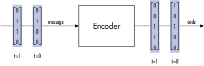
This example illustrates the encoder receiving a four-bit message and
producing a five-bit codeword at time 0. It repeats this process with a new
message at time 1.
For all coding techniques except Reed-Solomon using
binary input, the message vector must have length K and the corresponding
code vector has length N. For Reed-Solomon codes with binary input, the
symbols for the code are binary sequences of length M, corresponding to
elements of the Galois field GF(2M). In this
case, the message vector must have length M*K and the corresponding code
vector has length M*N. The Binary-Input RS Encoder block and the
Binary-Output RS Decoder block use this format for messages and
codewords.
If the input to a block-coding block is a frame-based vector, it must be a
column vector instead of a row vector.
To produce sample-based messages in the binary format, you can configure
the Bernoulli Binary Generator block
so that its Probability of a zero parameter is a vector
whose length is that of the signal you want to create. To produce
frame-based messages in the binary format, you can configure the same block
so that its Probability of a zero parameter is a scalar
and its Samples per frame parameter is the length of
the signal you want to create.
Using Serial Signals
If you prefer to structure messages and codewords as scalar signals, where
several samples jointly form a message word or codeword, you can use the
Buffer and Unbuffer blocks. Buffering
involves latency and multirate processing. If your model computes error
rates, the initial delay in the coding-buffering combination influences the
Receive delay parameter in the Error Rate Calculation block.
You can display the sample times of signals in your model. On the
tab, expand . In the
section, select . Alternatively, you can
attach Probe (Simulink) blocks to connector
lines to help evaluate sample timing, buffering, and delays.
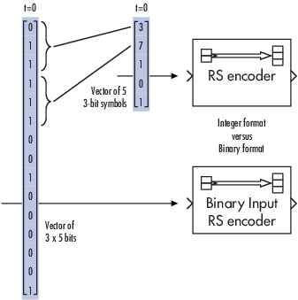
Integer Format (Reed-Solomon Only). A message word for an [N,K] Reed-Solomon code consists of M*K bits, which
you can interpret as K symbols from 0 to 2M. The
symbols are binary sequences of length M, corresponding to elements of the
Galois field GF(2M), in descending order of
powers. The integer format for Reed-Solomon codes lets you structure
messages and codewords as integer signals instead of
binary signals. (The input must be a frame-based column vector.)
Note
In this context, Simulink expects the first bit
to be the most significant bit in the symbol, as well as the smallest
index in a vector or the smallest time for a series of scalars.
The following figure illustrates the equivalence between binary and
integer signals for a Reed-Solomon encoder. The case for the decoder is
similar.
To produce sample-based messages in the integer format, you can configure
the Random Integer Generator block so that M-ary number
and Initial seed parameters are vectors of
the desired length and all entries of the M-ary number
vector are 2M. To produce frame-based messages in
the integer format, you can configure the same block so that its
M-ary number and Initial seed
parameters are scalars and its Samples per frame
parameter is the length of the signal you want to create.
Using Block Encoders and Decoders Within a Model
Once you have configured the coding blocks, a few tips can help you place them
correctly within your model:
-
If a block has multiple outputs, the first one is always the stream of
coding data.The Reed-Solomon and BCH blocks have an error counter as a second
output. -
Be sure that the signal sizes are appropriate for the mask parameters.
For example, if you use the Binary Cyclic Encoder block and set
Message length K to4,
the input signal must be a vector of length 4.You can display the size of signals in your model. On the
tab, expand
. In the
section, select
.
Examples of Block Coding
Example: Reed-Solomon Code in Integer Format. This example uses a Reed-Solomon code in integer format. It illustrates
the appropriate vector lengths of the code and message signals for the
coding blocks. It also exhibits error correction, using a simple way of
introducing errors into each codeword.

Open the model by typing doc_rscoding at the MATLAB
command line. To build the model, gather and configure these blocks:
-
Random Integer Generator,
in the Comm Sources library-
Set M-ary number to
15. -
Set Initial seed to a positive
number,randnis
chosen here. -
Check the Frame-based outputs check
box. -
Set Samples per frame to
5.
-
-
Integer-Input RS
Encoder-
Set Codeword length N to
15. -
Set Message length K to
5.
-
-
Gain (Simulink), in the
Simulink Math Operations library-
Set Gain to
[0; 0; 0; 0; 0;.
ones(10,1)]
-
-
Integer-Output RS
Decoder-
Set Codeword length N to
15. -
Set Message length K to
5.
-
-
Scope (Simulink), in the
Simulink Sinks library. Get two copies of this block. -
Add (Simulink), in the Simulink
Math Operations library-
Set List of signs to
|-+
-
Connect the blocks as shown in the preceding figure. On the
tab, in the
section, set Stop
time to 500. The
section appears on multiple
tabs.
You can display the vector length of signals in your model. On the
tab, expand . In the
section, select .
The encoder accepts a vector of length 5 (which is K in this case) and
produces a vector of length 15 (which is N in this case). The decoder does
the opposite.
Running the model produces the following scope images. The plotted error
count will vary based on the Initial Seed value used in
the Random Integer Generator block. You can adjust the axis range exactly
match that of the first scope. Right-click the plot area in the second scope
and select . On the
tab, adjust the axes limits.
Number of Errors Before Correction


The second plot is the number of errors that the decoder detected while
trying to recover the message. Often the number is five because the Gain
block replaces the first five symbols in each codeword with zeros. However,
the number of errors is less than five whenever a correct codeword contains
one or more zeros in the first five places.
The first plot is the difference between the original message and the
recovered message; since the decoder was able to correct all errors that
occurred, each of the five data streams in the plot is zero.
Notes on Specific Block-Coding Techniques
Although the Block Coding sublibrary is somewhat uniform in its look and feel,
the various coding techniques are not identical. This section describes special
options and restrictions that apply to parameters and signals for the coding
technique categories in this sublibrary. Coding techniques discussed below
include — Generic Linear Block code, Cyclic code, Hamming code, BCH code, and
Reed-Solomon code.
Generic Linear Block
Codes
Encoding a message using a generic linear block code requires a generator
matrix. Decoding the code requires the generator matrix and possibly a truth
table. To use the Binary Linear Encoder and Binary Linear Decoder blocks, you
must understand the Generator matrix and
Error-correction truth table parameters.
Generator Matrix — The process of encoding a message into
an [N,K] linear block code is determined by a K-by-N generator matrix
G. Specifically, a 1-by-K message vector
v is encoded into the 1-by-N codeword vector
vG. If G has the form
[Ik, P] or
[P, Ik], where
P is some K-by-(N-K) matrix and
Ik is the K-by-K identity matrix,
G is said to be in standard form.
(Some authors, such as Clark and Cain [2], use the first standard form, while others, such as Lin and Costello [3], use the second.) The linear block-coding blocks in this product require the
Generator matrix mask parameter to be in standard
form.
Decoding Table — A decoding table tells a decoder how to
correct errors that may have corrupted the code during transmission. Hamming
codes can correct any single-symbol error in any codeword. Other codes can
correct, or partially correct, errors that corrupt more than one symbol in a
given codeword.
The Binary Linear Decoder block allows
you to specify a decoding table in the Error-correction truth
table parameter. Represent a decoding table as a matrix with N
columns and 2N-K rows. Each row gives a correction
vector for one received codeword vector.
You can avoid specifying a decoding table explicitly, by setting the
Error-correction truth table parameter to
0. When Error-correction truth table
is 0, the block computes a decoding table using the syndtable function.
Cyclic Codes
For cyclic codes, the codeword length N must have the form
2M-1, where M is an integer greater than or equal
to 3.
Generator Polynomials — Cyclic codes have special
algebraic properties that allow a polynomial to determine the coding process
completely. This so-called generator polynomial is a degree-(N-K) divisor of the
polynomial xN-1. Van Lint [5] explains how a generator polynomial determines a cyclic code.
The Binary Cyclic Encoder and Binary Cyclic Decoder blocks allow
you to specify a generator polynomial as the second mask parameter, instead of
specifying K there. The blocks represent a generator polynomial using a vector
that lists the coefficients of the polynomial in order of
ascending powers of the variable. You can find
generator polynomials for cyclic codes using the cyclpoly function.
If you do not want to specify a generator polynomial, set the second mask
parameter to the value of K.
Hamming Codes
For Hamming codes, the codeword length N must have the form
2M-1, where M is an integer greater than or equal
to 3. The message length K must equal N-M.
Primitive Polynomials — Hamming codes rely on algebraic
fields that have 2M elements (or, more generally,
pM elements for a prime number
p). Elements of such fields are named relative
to a distinguished element of the field that is called a
primitive element. The minimal polynomial of a
primitive element is called a primitive polynomial. The
Hamming Encoder and Hamming Decoder blocks allow you to
specify a primitive polynomial for the finite field that they use for
computations. If you want to specify this polynomial, do so in the second mask
parameter field. The blocks represent a primitive polynomial using a vector that
lists the coefficients of the polynomial in order of
ascending powers of the variable. You can find
generator polynomials for Galois fields using the gfprimfd function.
If you do not want to specify a primitive polynomial, set the second mask
parameter to the value of K.
BCH Codes
BCH codes are cyclic error-correcting codes that are constructed using finite
fields. For these codes, the codeword length N must have the form
2M-1, where M is an integer from 3 to 9. The
message length K is restricted to particular values that depend on N. To see
which values of K are valid for a given N, see the comm.BCHEncoder
System object™ reference page. No known analytic formula describes the
relationship among the codeword length, message length, and error-correction
capability for BCH codes.
Narrow-Sense BCH Codes
The narrow-sense generator polynomial is LCM[m_1(x), m_2(x), …, m_2t(x)],
where:
-
LCM represents the least common multiple,
-
m_i(x) represents the minimum polynomial corresponding to
αi, α is a root of the default primitive
polynomial for the field GF(n+1), -
and t represents the error-correcting capability of the code.
Reed-Solomon Codes
Reed-Solomon codes are useful for correcting errors that occur in bursts. In
the simplest case, the length of codewords in a Reed-Solomon code is of the form
N= 2M-1, where the 2M is
the number of symbols for the code. The error-correction capability of a
Reed-Solomon code is floor((N-K)/2), where K is the length of
message words. The difference N-K must be even.
It is sometimes convenient to use a shortened Reed-Solomon code in which N is
less than 2M-1. In this case, the encoder appends
2M-1-N zero symbols to each message word and
codeword. The error-correction capability of a shortened Reed-Solomon code is
also floor((N-K)/2). The Communications Toolbox Reed-Solomon blocks can implement shortened Reed-Solomon
codes.
Effect of Nonbinary Symbols — One difference between
Reed-Solomon codes and the other codes supported in this product is that
Reed-Solomon codes process symbols in GF(2M) instead
of GF(2). M bits specify each symbol. The nonbinary nature of the Reed-Solomon
code symbols causes the Reed-Solomon blocks to differ from other coding blocks
in these ways:
-
You can use the integer format, via the Integer-Input RS Encoder and
Integer-Output RS Decoder
blocks. -
The binary format expects the vector lengths to be an integer multiple
of M*K (not K) for messages and the same integer M*N (not N) for
codewords.
Error Information — The Reed-Solomon decoding blocks
(Binary-Output RS Decoder and Integer-Output RS Decoder) return
error-related information during the simulation. The second output signal
indicates the number of errors that the block detected in the input codeword. A
-1 in the second output indicates that the block detected more errors than it
could correct using the coding scheme.
Shortening, Puncturing, and Erasures
Many standards utilize punctured codes, and digital receivers can easily
output erasures. BCH and RS performance improves significantly in fading
channels where the receiver generates erasures.
A punctured codeword has only parity symbols removed, and
a shortened codeword has only information symbols removed.
A codeword with erasures can have those erasures in either information symbols
or parity symbols.
Reed Solomon Examples with Shortening, Puncturing, and
Erasures
In this section, a representative example of Reed Solomon coding with
shortening, puncturing, and erasures is built with increasing complexity of
error correction.
Encoder Example with Shortening and
Puncturing
The following figure shows a representative example of a (7,3) Reed Solomon
encoder with shortening and puncturing.
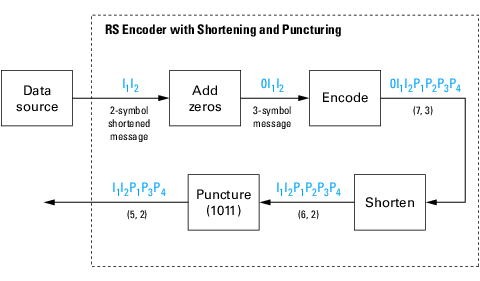
In this figure, the message source outputs two information symbols, designated
by I1I2. (For a BCH example, the
symbols are binary bits.) Because the code is a shortened (7,3) code, a zero
must be added ahead of the information symbols, yielding a three-symbol message
of 0I1I2. The modified message
sequence is RS encoded, and the added information zero is then removed, which
yields a result of
I1I2P1P2P3P4.
(In this example, the parity bits are at the end of the codeword.)
The puncturing operation is governed by the puncture vector, which, in this
case, is 1011. Within the puncture vector, a 1 means that the
symbol is kept, and a 0 means that the symbol is thrown away.
In this example, the puncturing operation removes the second parity symbol,
yielding a final vector of
I1I2P1P3P4.
Decoder Example with Shortening and
Puncturing
The following figure shows how the RS decoder operates on a shortened and
punctured codeword.
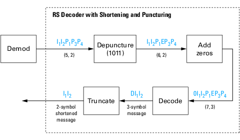
This case corresponds to the encoder operations shown in the figure of the RS
encoder with shortening and puncturing. As shown in the preceding figure, the
encoder receives a (5,2) codeword, because it has been shortened from a (7,3)
codeword by one symbol, and one symbol has also been punctured.
As a first step, the decoder adds an erasure, designated by E, in the second
parity position of the codeword. This corresponds to the puncture vector 1011.
Adding a zero accounts for shortening, in the same way as shown in the preceding
figure. The single erasure does not exceed the erasure-correcting capability of
the code, which can correct four erasures. The decoding operation results in the
three-symbol message DI1I2. The
first symbol is truncated, as in the preceding figure, yielding a final output
of I1I2.
Decoder Example with Shortening, Puncturing, and
Erasures
The following figure shows the decoder operating on the punctured, shortened
codeword, while also correcting erasures generated by the receiver.

In this figure, demodulator receives the
I1I2P1P3P4
vector that the encoder sent. The demodulator declares that two of the five
received symbols are unreliable enough to be erased, such that symbols 2 and 5
are deemed to be erasures. The 01001 vector, provided by an external source,
indicates these erasures. Within the erasures vector, a 1 means that the symbol
is to be replaced with an erasure symbol, and a 0 means that the symbol is
passed unaltered.
The decoder blocks receive the codeword and the erasure vector, and perform
the erasures indicated by the vector 01001. Within the erasures vector, a 1
means that the symbol is to be replaced with an erasure symbol, and a 0 means
that the symbol is passed unaltered. The resulting codeword vector is
I1EP1P3E,
where E is an erasure symbol.
The codeword is then depunctured, according to the puncture vector used in the
encoding operation (i.e., 1011). Thus, an erasure symbol is inserted between
P1 and P3, yielding a codeword
vector of
I1EP1EP3E.
Just prior to decoding, the addition of zeros at the beginning of the
information vector accounts for the shortening. The resulting vector is
0I1EP1EP3E,
such that a (7,3) codeword is sent to the Berlekamp algorithm.
This codeword is decoded, yielding a three-symbol message of
DI1I2 (where D refers to a
dummy symbol). Finally, the removal of the D symbol from the message vector
accounts for the shortening and yields the original
I1I2 vector.
For additional information, see the Reed-Solomon Coding with Erasures, Punctures, and Shortening
MATLAB example or the Reed-Solomon Coding with Erasures, Punctures, and Shortening in Simulink
example.
Reed-Solomon Code in Integer Format
To open an example model that uses a Reed-Solomon code in integer format, type
doc_rscoding at the MATLAB command line. For more information about the model, see Example: Reed-Solomon Code in Integer Format
Find a Generator Polynomial
To find a generator polynomial for a cyclic, BCH, or Reed-Solomon code, use
the cyclpoly, bchgenpoly, or
rsgenpoly function, respectively. The commands
genpolyCyclic = cyclpoly(15,5) % 1+X^5+X^10
genpolyBCH = bchgenpoly(15,5)  % x^10+x^8+x^5+x^4+x^2+x+1
genpolyRS = rsgenpoly(15,5)
find generator polynomials for block codes of different types. The output is
below.
genpolyCyclic =

     1     0     0     0     0     1     0     0     0     0     1


genpolyBCH = GF(2) array.

Array elements =

     1     0     1     0     0     1     1     0     1     1     1


genpolyRS = GF(2^4) array. Primitive polynomial = D^4+D+1 (19 decimal)

Array elements =

     1     4     8    10    12     9     4     2    12     2     7
The formats of these outputs vary:
-
cyclpolyrepresents a generator polynomial using
an integer row vector that lists the polynomial’s coefficients in order
of ascending powers of the variable. -
bchgenpolyandrsgenpoly
represent a generator polynomial using a Galois row vector that lists
the polynomial’s coefficients in order of
descending powers of the variable. -
rsgenpolyuses coefficients in a Galois field
other than the binary field GF(2). For more information on the meaning
of these coefficients, see How Integers Correspond to Galois Field Elements and Polynomials over Galois Fields.
Nonuniqueness of Generator Polynomials
Some pairs of message length and codeword length do not uniquely determine the
generator polynomial. The syntaxes for functions in the example above also
include options for retrieving generator polynomials that satisfy certain
constraints that you specify. See the functions’ reference pages for details
about syntax options.
Algebraic Expression for Generator
Polynomials
The generator polynomials produced by bchgenpoly and
rsgenpoly have the form
(X — Ab)(X — Ab+1)…(X — Ab+2t-1),
where A is a primitive element for an appropriate Galois field, and b and t are
integers. See the functions’ reference pages for more information about this
expression.
Performing Other Block Code Tasks
This section describes functions that compute typical parameters associated
with linear block codes, as well as functions that convert information from one
format to another.
-
Error Correction Versus Error Detection for
Linear Block CodesYou can use a linear block code to detect
dmin -1 errors or to
correct t = [12(dmin−1)] errors.If you compromise the error correction capability of a code, you
can detect more than t errors. For example, a
code with dmin = 7 can
correct t = 3 errors or it can detect up to 4
errors and correct up to 2 errors. -
Finding the Error-Correction
CapabilityThe
bchgenpolyand
rsgenpolyfunctions can return an optional
second output argument that indicates the error-correction
capability of a BCH or Reed-Solomon code. For example, the
commands[g,t] = bchgenpoly(31,16); t t = 3find that a [31, 16] BCH code can correct up to three errors in
each codeword. -
Finding Generator and Parity-Check
MatricesTo find a parity-check and generator matrix for a Hamming code
with codeword length2^m-1, use the
hammgenfunction as below.
mmust be at least three.[parmat,genmat] = hammgen(m); % Hamming
To find a parity-check and generator matrix for a cyclic code, use
thecyclgenfunction. You must provide the
codeword length and a valid generator polynomial. You can use the
cyclpolyfunction to produce one possible
generator polynomial after you provide the codeword length and
message length. For example,[parmat,genmat] = cyclgen(7,cyclpoly(7,4)); % Cyclic -
Converting Between Parity-Check and
Generator MatricesThe
gen2parfunction converts a generator
matrix into a parity-check matrix, and vice versa. The reference
page forgen2parcontains examples to
illustrate this.
Selected Bibliography for Block Coding
[1] Berlekamp, Elwyn R., Algebraic Coding
Theory, New York, McGraw-Hill, 1968.
[2] Clark, George C. Jr., and J. Bibb Cain,
Error-Correction Coding for Digital
Communications, New York, Plenum Press, 1981.
[3] Lin, Shu, and Daniel J. Costello, Jr.,
Error Control Coding: Fundamentals and
Applications, Englewood Cliffs, NJ, Prentice-Hall,
1983.
[4] Peterson, W. Wesley, and E. J. Weldon, Jr.,
Error-Correcting Codes, 2nd ed., Cambridge, MA,
MIT Press, 1972.
[5] van Lint, J. H., Introduction to Coding
Theory, New York, Springer-Verlag, 1982.
[6] Wicker, Stephen B., Error Control
Systems for Digital Communication and Storage, Upper Saddle
River, NJ, Prentice Hall, 1995.
[7] Gallager, Robert G., Low-Density
Parity-Check Codes, Cambridge, MA, MIT Press,
1963.
[8] Ryan, William E., “An introduction to
LDPC codes,” Coding and Signal Processing for Magnetic
Recoding Systems (Vasic, B., ed.), CRC Press,
2004.
Convolutional Codes
-
Convolutional Code Features
-
Polynomial Description of a Convolutional Code
-
Trellis Description of a Convolutional Code
-
Create and Decode Convolutional Codes
-
Design a Rate-2/3 Feedforward Encoder Using MATLAB
-
Design a Rate 2/3 Feedforward Encoder Using Simulink
-
Puncture a Convolutional Code Using MATLAB
-
Implement a Systematic Encoder with Feedback Using Simulink
-
Soft-Decision Decoding
-
Tailbiting Encoding Using Feedback
Encoders -
Selected Bibliography for Convolutional Coding
Convolutional Code Features
Convolutional coding is a special case of error-control coding. Unlike a block
coder, a convolutional coder is not a memoryless device. Even though a
convolutional coder accepts a fixed number of message symbols and produces a
fixed number of code symbols, its computations depend not only on the current
set of input symbols but on some of the previous input symbols.
Communications Toolbox provides convolutional coding capabilities as Simulink blocks, System objects, and MATLAB functions. This product supports feedforward and feedback
convolutional codes that can be described by a trellis structure or a set of
generator polynomials. It uses the Viterbi algorithm to implement hard-decision
and soft-decision decoding.
The product also includes an a posteriori probability
decoder, which can be used for soft output decoding of convolutional
codes.
For background information about convolutional coding, see the works listed in
Selected Bibliography
for Convolutional Coding.
Block Parameters for Convolutional
Coding
To process convolutional codes, use the Convolutional Encoder, Viterbi Decoder, and/or APP Decoder blocks in the
Convolutional sublibrary. If a mask parameter is required in both the encoder
and the decoder, use the same value in both blocks.
The blocks in the Convolutional sublibrary assume that you use one of two
different representations of a convolutional encoder:
-
If you design your encoder using a diagram with shift registers and
modulo-2 adders, you can compute the code generator polynomial matrix
and subsequently use thepoly2trellisfunction (in
Communications Toolbox) to generate the corresponding trellis structure mask
parameter automatically. For an example, see Design a Rate 2/3 Feedforward Encoder Using Simulink. -
If you design your encoder using a trellis diagram, you can construct
the trellis structure in MATLAB and use it as the mask parameter.
For more information about these representations, see Polynomial
Description of a Convolutional Code and Trellis Description of
a Convolutional Code.
Using the Polynomial Description in
Blocks
To use the polynomial description with the Convolutional Encoder, Viterbi Decoder, or APP Decoder blocks, use the utility
function poly2trellis from Communications Toolbox. This function accepts a polynomial description and converts it
into a trellis description. For example, the following command computes the
trellis description of an encoder whose constraint length is 5 and whose
generator polynomials are 35 and 31:
trellis = poly2trellis(5,[35 31]);
To use this encoder with one of the convolutional-coding blocks, simply place
a poly2trellis command such as
in the Trellis structure parameter field.
Polynomial Description of a Convolutional Code
A polynomial description of a convolutional encoder describes the connections
among shift registers and modulo 2 adders. For example, the figure below depicts
a feedforward convolutional encoder that has one input, two outputs, and two
shift registers.

A polynomial description of a convolutional encoder has either two or three
components, depending on whether the encoder is a feedforward or feedback
type:
-
Constraint
lengths -
Generator
polynomials -
Feedback connection
polynomials (for feedback encoders only)
Constraint Lengths. The constraint lengths of the encoder form a vector whose length is the
number of inputs in the encoder diagram. The elements of this vector
indicate the number of bits stored in each shift register,
including the current input bits.
In the figure above, the constraint length is three. It is a scalar
because the encoder has one input stream, and its value is one plus the
number of shift registers for that input.
Generator Polynomials. If the encoder diagram has k inputs and n outputs, the code generator
matrix is a k-by-n matrix. The element in the ith row and jth column
indicates how the ith input contributes to the jth output.
For systematic bits of a systematic feedback encoder,
match the entry in the code generator matrix with the corresponding element
of the feedback connection vector. See Feedback Connection Polynomials below for details.
In other situations, you can determine the (i,j) entry in the matrix as
follows:
-
Build a binary number representation by placing a 1 in each spot
where a connection line from the shift register feeds into the
adder, and a 0 elsewhere. The leftmost spot in the binary number
represents the current input, while the rightmost spot represents
the oldest input that still remains in the shift register. -
Convert this binary representation into an octal representation by
considering consecutive triplets of bits, starting from the
rightmost bit. The rightmost bit in each triplet is the least
significant. If the number of bits is not a multiple of three, place
zero bits at the left end as necessary. (For example, interpret
1101010 as 001 101 010 and convert it to 152.)
For example, the binary numbers corresponding to the upper and lower
adders in the figure above are 110 and 111, respectively. These binary
numbers are equivalent to the octal numbers 6 and 7, respectively, so the
generator polynomial matrix is [6 7].
Note
You can perform the binary-to-octal conversion in MATLAB by using code like
str2num(dec2base(bin2dec('110'),8)).
For a table of some good convolutional code generators, refer to [2] in the section Selected Bibliography for Block Coding, especially that book’s
appendices.
Feedback Connection Polynomials. If you are representing a feedback encoder, you need a vector of feedback
connection polynomials. The length of this vector is the number of inputs in
the encoder diagram. The elements of this vector indicate the feedback
connection for each input, using an octal format. First build a binary
number representation as in step 1 above. Then convert the binary
representation into an octal representation as in step 2 above.
If the encoder has a feedback configuration and is also systematic, the
code generator and feedback connection parameters corresponding to the
systematic bits must have the same values.
Use Trellis Structure for Rate 1/2 Feedback Convolutional Encoder
Create a trellis structure to represent the rate 1/2 systematic convolutional encoder with feedback shown in this diagram.
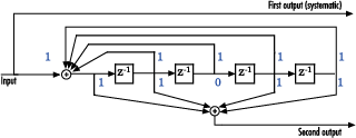
This encoder has 5 for its constraint length, [37 33] as its generator polynomial matrix, and 37 for its feedback connection polynomial.
The first generator polynomial is octal 37. The second generator polynomial is octal 33. The feedback polynomial is octal 37. The first generator polynomial matches the feedback connection polynomial because the first output corresponds to the systematic bits.
The binary vector [1 1 1 1 1] represents octal 37 and corresponds to the upper row of binary digits in the diagram. The binary vector [1 1 0 1 1] represents octal 33 and corresponds to the lower row of binary digits in the diagram. These binary digits indicate connections from the outputs of the registers to the two adders in the diagram. The initial 1 corresponds to the input bit.
Convert the polynomial to a trellis structure by using the poly2trellis function. When used with a feedback polynomial, poly2trellis makes a feedback connection to the input of the trellis.
trellis = poly2trellis(5,[37 33],37)
trellis = struct with fields:
     numInputSymbols: 2
    numOutputSymbols: 4
           numStates: 16
          nextStates: [16x2 double]
             outputs: [16x2 double]
Generate random binary data. Convolutionally encode the data by using the specified trellis structure. Decode the coded data by using the Viterbi algorithm with the specified trellis structure, 34 for its traceback depth, truncated operation mode, and hard decisions.
data = randi([0 1],70,1);
codedData = convenc(data,trellis);
tbdepth = 34; % Traceback depth for Viterbi decoder
decodedData = vitdec(codedData,trellis,tbdepth,'trunc','hard');
Verify the decoded data has zero bit errors.
Using the Polynomial Description in MATLAB. To use the polynomial description with the functions
convenc and vitdec, first
convert it into a trellis description using the
poly2trellis function. For example, the command
below computes the trellis description of the encoder pictured in the
section Polynomial
Description of a Convolutional Code.
trellis = poly2trellis(3,[6 7]);
The MATLAB structure trellis is a suitable input
argument for convenc and
vitdec.
Trellis Description of a Convolutional Code
A trellis description of a convolutional encoder shows how each possible input
to the encoder influences both the output and the state transitions of the
encoder. This section describes trellises, and how to represent
trellises in MATLAB, and gives an example of a MATLAB
trellis.
The figure below depicts a trellis for the convolutional encoder from the
previous section. The encoder has four states (numbered in binary from 00 to
11), a one-bit input, and a two-bit output. (The ratio of input bits to output
bits makes this encoder a rate-1/2 encoder.) Each solid arrow shows how the
encoder changes its state if the current input is zero, and each dashed arrow
shows how the encoder changes its state if the current input is one. The octal
numbers above each arrow indicate the current output of the encoder.
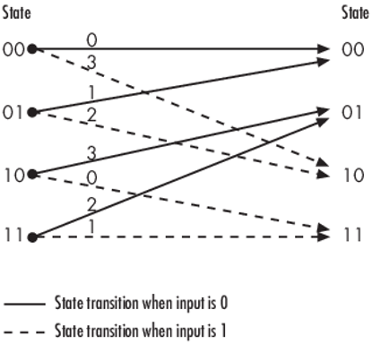
As an example of interpreting this trellis diagram, if the encoder is in the
10 state and receives an input of zero, it outputs the code symbol 3 and changes
to the 01 state. If it is in the 10 state and receives an input of one, it
outputs the code symbol 0 and changes to the 11 state.
Note that any polynomial description of a convolutional encoder is equivalent
to some trellis description, although some trellises have no corresponding
polynomial descriptions.
Specifying a Trellis in MATLAB. To specify a trellis in MATLAB, use a specific form of a MATLAB structure called a trellis structure. A trellis structure must
have five fields, as in the table below.
Fields of a Trellis Structure for a Rate k/n Code
| Field in Trellis Structure |
Dimensions | Meaning |
|---|---|---|
numInputSymbols
|
Scalar | Number of input symbols to the encoder: 2k |
numOutputsymbols
|
Scalar | Number of output symbols from the encoder: 2n |
numStates
|
Scalar | Number of states in the encoder |
nextStates
|
numStates-by-2kmatrix |
Next states for all combinations of current state and current input |
outputs
|
numStates-by-2kmatrix |
Outputs (in octal) for all combinations of current state and current input |
Note
While your trellis structure can have any name, its fields must have
the exact names as in the table. Field names are
case sensitive.
In the nextStates matrix, each entry is an integer
between 0 and numStates-1. The element in the ith row and
jth column denotes the next state when the starting state is i-1 and the
input bits have decimal representation j-1. To convert the input bits to a
decimal value, use the first input bit as the most significant bit (MSB).
For example, the second column of the nextStates matrix
stores the next states when the current set of input values is {0,…,0,1}.
To learn how to assign numbers to states, see the reference page for
istrellis.
In the outputs matrix, the element in the ith row and
jth column denotes the encoder’s output when the starting state is i-1 and
the input bits have decimal representation j-1. To convert to decimal value,
use the first output bit as the MSB.
How to Create a MATLAB Trellis Structure. Once you know what information you want to put into each field, you can
create a trellis structure in any of these ways:
-
Define each of the five fields individually, using
structurename.fieldnamenotation. For
example, set the first field of a structure called
susing the command below. Use additional
commands to define the other fields.The reference page for the
istrellisfunction
illustrates this approach. -
Collect all field names and their values in a single
structcommand. For example:s = struct('numInputSymbols',2,'numOutputSymbols',2,... 'numStates',2,'nextStates',[0 1;0 1],'outputs',[0 0;1 1]); -
Start with a polynomial description of the encoder and use the
poly2trellisfunction to convert it to a
valid trellis structure. For more information , see Polynomial Description of a Convolutional Code.
To check whether your structure is a valid trellis structure, use the
istrellis function.
Example: A MATLAB Trellis Structure. Consider the trellis shown below.
To build a trellis structure that describes it, use the command
below.
trellis = struct('numInputSymbols',2,'numOutputSymbols',4,...
'numStates',4,'nextStates',[0 2;0 2;1 3;1 3],...
'outputs',[0 3;1 2;3 0;2 1]);
The number of input symbols is 2 because the trellis diagram has two types
of input path: the solid arrow and the dashed arrow. The number of output
symbols is 4 because the numbers above the arrows can be either 0, 1, 2, or
3. The number of states is 4 because there are four bullets on the left side
of the trellis diagram (equivalently, four on the right side). To compute
the matrix of next states, create a matrix whose rows correspond to the four
current states on the left side of the trellis, whose columns correspond to
the inputs of 0 and 1, and whose elements give the next states at the end of
the arrows on the right side of the trellis. To compute the matrix of
outputs, create a matrix whose rows and columns are as in the next states
matrix, but whose elements give the octal outputs shown above the arrows in
the trellis.
Create and Decode Convolutional Codes
The functions for encoding and decoding convolutional codes are
convenc and vitdec. This section
discusses using these functions to create and decode convolutional codes.
Encoding. A simple way to use convenc to create a convolutional
code is shown in the commands below.
% Define a trellis.
t = poly2trellis([4 3],[4 5 17;7 4 2]);
% Encode a vector of ones.
x = ones(100,1);
code = convenc(x,t);
The first command converts a polynomial description of a feedforward
convolutional encoder to the corresponding trellis description. The second
command encodes 100 bits, or 50 two-bit symbols. Because the code rate in
this example is 2/3, the output vector code contains 150
bits (that is, 100 input bits times 3/2).
To check whether your trellis corresponds to a catastrophic convolutional
code, use the iscatastrophic function.
Hard-Decision Decoding. To decode using hard decisions, use the vitdec
function with the flag 'hard' and with
binary input data. Because the output of
convenc is binary, hard-decision decoding can use
the output of convenc directly, without additional
processing. This example extends the previous example and implements
hard-decision decoding.
Define a trellis.

t = poly2trellis([4 3],[4 5 17;7 4 2]);
Encode a vector of ones.

code = convenc(ones(100,1),t);
Set the traceback length for decoding and decode using vitdec.

tb = 2;
decoded = vitdec(code,t,tb,'trunc','hard');
Verify that the decoded data is a vector of 100 ones.

isequal(decoded,ones(100,1))
Soft-Decision Decoding. To decode using soft decisions, use the vitdec
function with the flag 'soft'. Specify the number,
nsdec, of soft-decision bits and use input data
consisting of integers between 0 and 2^nsdec-1.
An input of 0 represents the most confident 0, while an input of
2^nsdec-1 represents the most confident 1. Other
values represent less confident decisions. For example, the table below
lists interpretations of values for 3-bit soft decisions.
Input Values for 3-bit Soft Decisions
| Input Value | Interpretation |
|---|---|
| 0 | Most confident 0 |
| 1 | Second most confident 0 |
| 2 | Third most confident 0 |
| 3 | Least confident 0 |
| 4 | Least confident 1 |
| 5 | Third most confident 1 |
| 6 | Second most confident 1 |
| 7 | Most confident 1 |
Implement Soft-Decision Decoding Using
MATLAB
The script below illustrates decoding with 3-bit soft decisions. First it
creates a convolutional code with convenc and adds
white Gaussian noise to the code with awgn. Then, to
prepare for soft-decision decoding, the example uses
quantiz to map the noisy data values to appropriate
decision-value integers between 0 and 7. The second argument in
quantiz is a partition vector that determines which
data values map to 0, 1, 2, etc. The partition is chosen so that values near
0 map to 0, and values near 1 map to 7. (You can refine the partition to
obtain better decoding performance if your application requires it.)
Finally, the example decodes the code and computes the bit error rate. When
comparing the decoded data with the original message, the example must take
the decoding delay into account. The continuous operation mode of
vitdec causes a delay equal to the traceback
length, so msg(1) corresponds to
decoded(tblen+1) rather than to
decoded(1).
s = RandStream.create('mt19937ar', 'seed',94384);
prevStream = RandStream.setGlobalStream(s);
msg = randi([0 1],4000,1); % Random data
t = poly2trellis(7,[171 133]); % Define trellis.
% Create a ConvolutionalEncoder System object
hConvEnc = comm.ConvolutionalEncoder(t);
% Create an AWGNChannel System object.
hChan = comm.AWGNChannel('NoiseMethod', 'Signal to noise ratio (SNR)',...
  'SNR', 6);
% Create a ViterbiDecoder System object
hVitDec = comm.ViterbiDecoder(t, 'InputFormat', 'Soft', ...
    'SoftInputWordLength', 3, 'TracebackDepth', 48, ...
    'TerminationMethod', 'Continuous');
% Create a ErrorRate Calculator System object. Account for the receive
% delay caused by the traceback length of the viterbi decoder.
hErrorCalc = comm.ErrorRate('ReceiveDelay', 48);
ber = zeros(3,1); % Store BER values
code = step(hConvEnc,msg); % Encode the data.
hChan.SignalPower = (code'*code)/length(code);
ncode = step(hChan,code); % Add noise.

% Quantize to prepare for soft-decision decoding.
qcode = quantiz(ncode,[0.001,.1,.3,.5,.7,.9,.999]);

tblen = 48; delay = tblen; % Traceback length
decoded = step(hVitDec,qcode); % Decode.

% Compute bit error rate.
ber = step(hErrorCalc, msg, decoded);
ratio = ber(1)
number = ber(2)
RandStream.setGlobalStream(prevStream);
The output is below.
number =

     5


ratio =

    0.0013
Implement Soft-Decision Decoding Using Simulink. This example creates a rate 1/2 convolutional code. It uses a quantizer
and the Viterbi Decoder block to perform soft-decision decoding. To open the
model, enter doc_softdecision at the MATLAB command line. For a description of the model, see Overview
of the Simulation.
Defining the Convolutional Code
The feedforward convolutional encoder in this example is depicted
below.
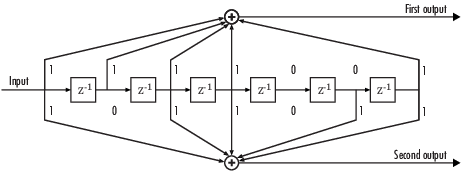
The encoder’s constraint length is a scalar since the encoder has one
input. The value of the constraint length is the number of bits stored in
the shift register, including the current input. There are six memory
registers, and the current input is one bit. Thus the constraint length of
the code is 7.
The code generator is a 1-by-2 matrix of octal numbers because the encoder
has one input and two outputs. The first element in the matrix indicates
which input values contribute to the first output, and the second element in
the matrix indicates which input values contribute to the second
output.
For example, the first output in the encoder diagram is the modulo-2 sum
of the rightmost and the four leftmost elements in the diagram’s array of
input values. The seven-digit binary number 1111001 captures this
information, and is equivalent to the octal number 171. The octal number 171
thus becomes the first entry of the code generator matrix. Here, each
triplet of bits uses the leftmost bit as the most significant bit. The
second output corresponds to the binary number 1011011, which is equivalent
to the octal number 133. The code generator is therefore
[171 133].
The Trellis structure parameter in the Convolutional
Encoder block tells the block which code to use when processing data. In
this case, the poly2trellis function, in
Communications Toolbox, converts the constraint length and the pair of octal numbers
into a valid trellis structure.
While the message data entering the Convolutional Encoder block is a
scalar bit stream, the encoded data leaving the block is a stream of binary
vectors of length 2.
Mapping the Received Data
The received data, that is, the output of the AWGN Channel block, consists
of complex numbers that are close to -1 and 1. In order to reconstruct the
original binary message, the receiver part of the model must decode the
convolutional code. The Viterbi Decoder block in this model expects its
input data to be integers between 0 and 7. The demodulator, a custom
subsystem in this model, transforms the received data into a format that the
Viterbi Decoder block can interpret properly. More specifically, the
demodulator subsystem
-
Converts the received data signal to a real signal by removing its
imaginary part. It is reasonable to assume that the imaginary part
of the received data does not contain essential information, because
the imaginary part of the transmitted data is zero (ignoring small
roundoff errors) and because the channel noise is not very
powerful. -
Normalizes the received data by dividing by the standard deviation
of the noise estimate and then multiplying by -1. -
Quantizes the normalized data using three bits.
The combination of this mapping and the Viterbi Decoder block’s decision
mapping reverses the BPSK modulation that the BPSK Modulator Baseband block
performs on the transmitting side of this model. To examine the demodulator
subsystem in more detail, double-click the icon labeled Soft-Output BPSK
Demodulator.
Decoding the Convolutional Code
After the received data is properly mapped to length-2 vectors of 3-bit
decision values, the Viterbi Decoder block decodes it. The block uses a
soft-decision algorithm with 23 different input
values because the Decision type parameter is
Soft Decision and the Number of
soft decision bits parameter is 3.
Soft-Decision Interpretation of
Data
When the Decision type parameter is set to
Soft Decision, the Viterbi Decoder block
requires input values between 0 and 2b-1, where
b is the Number of soft decision
bits parameter. The block interprets 0 as the most confident
decision that the codeword bit is a 0 and interprets
2b-1 as the most confident decision that the
codeword bit is a 1. The values in between these extremes represent less
confident decisions. The following table lists the interpretations of the
eight possible input values for this example.
| Decision Value | Interpretation |
|---|---|
| 0 | Most confident 0 |
| 1 | Second most confident 0 |
| 2 | Third most confident 0 |
| 3 | Least confident 0 |
| 4 | Least confident 1 |
| 5 | Third most confident 1 |
| 6 | Second most confident 1 |
| 7 | Most confident 1 |
Traceback and Decoding Delay
The traceback depth influences the decoding delay. The decoding delay is the number of zero symbols that precede the first decoded symbol in the output.
-
For the continuous operating mode, the decoding delay is equal to the number of
traceback depth symbols. -
For the truncated or terminated operating mode, the decoding delay is zero. In
this case, the traceback depth must be less than or equal to the number of symbols
in each input.
Traceback Depth Estimate
As a general estimate, a typical traceback depth value is approximately two
to three times (ConstraintLength – 1) / (1 –
coderate). The constraint length of the code, ConstraintLength,
is equal to (log2(trellis.numStates) +
1). The coderate is equal to (K / N) ×
(length(PuncturePattern) /
sum(PuncturePattern).
K is the number of input symbols, N
is the number of output symbols, and PuncturePattern is the puncture
pattern vector.
For example, applying this general estimate, results in these approximate
traceback depths.
-
A rate 1/2 code has a traceback depth of 5(ConstraintLength – 1).
-
A rate 2/3 code has a traceback depth of 7.5(ConstraintLength – 1).
-
A rate 3/4 code has a traceback depth of 10(ConstraintLength – 1).
-
A rate 5/6 code has a traceback depth of 15(ConstraintLength – 1).
The Traceback depth parameter in the Viterbi Decoder block represents
the length of the decoding delay. Some hardware implementations offer
options of 48 and 96. This example chooses 48 because that is closer to the
estimated target for a rate ½ code with a constraint length of 7.
Delay in Received Data
The Receive delay parameter of the Error Rate Calculation block is
nonzero because a given message bit and its corresponding recovered bit are
separated in time by a nonzero amount of simulation time. The
Receive delay parameter tells the block which
elements of its input signals to compare when checking for errors.
In this case, the Receive delay value is equal to the Traceback depth
value (48).
Comparing Simulation Results with Theoretical
Results
This section describes how to compare the bit error rate in this
simulation with the bit error rate that would theoretically result from
unquantized decoding. The process includes these steps
-
Computing Theoretical Bounds for the Bit
Error RateTo calculate theoretical bounds for the bit error rate
Pb of the
convolutional code in this model, you can use this estimate
based on unquantized-decision decoding:In this estimate,
cd is the sum of
bit errors for error events of distance d,
and f is the free distance of the code. The
quantity Pd is the
pairwise error probability, given bywhere R is the code rate of 1/2, and
erfcis the
MATLAB complementary error function, defined byValues for the coefficients
cd and the free
distance f are in published articles such
as «Convolutional Codes with Optimum Distance Spectrum» [3]. The free distance for this code is
f = 10.The following commands calculate the values of
Pb for
Eb/N0
values in the range from 1 to 4, in increments of 0.5:EbNoVec = [1:0.5:4.0]; R = 1/2; % Errs is the vector of sums of bit errors for % error events at distance d, for d from 10 to 29. Errs = [36 0 211 0 1404 0 11633 0 77433 0 502690 0,... 3322763 0 21292910 0 134365911 0 843425871 0]; % P is the matrix of pairwise error probilities, for % Eb/No values in EbNoVec and d from 10 to 29. P = zeros(20,7); % Initialize. for d = 10:29 P(d-9,:) = (1/2)*erfc(sqrt(d*R*10.^(EbNoVec/10))); end % Bounds is the vector of upper bounds for the bit error % rate, for Eb/No values in EbNoVec. Bounds = Errs*P;
-
Simulating Multiple Times to Collect Bit
Error RatesYou can efficiently vary the simulation parameters by using
thesim(Simulink) function to
run the simulation from the MATLAB command line. For example, the following code
calculates the bit error rate at bit energy-to-noise ratios
ranging from 1 dB to 4 dB, in increments of 0.5 dB. It collects
all bit error rates from these simulations in the matrix
BERVec. It also plots the bit error rates
in a figure window along with the theoretical bounds computed in
the preceding code fragment.Note
To simulate the model, enter
doc_softdecisionat the MATLAB command line. Then execute these commands,
which might take a few minutes.% Plot theoretical bounds and set up figure. figure; semilogy(EbNoVec,Bounds,'bo',1,NaN,'r*'); xlabel('Eb/No (dB)'); ylabel('Bit Error Rate'); title('Bit Error Rate (BER)'); l = legend('Theoretical bound on BER','Actual BER'); l.AutoUpdate = 'off'; axis([1 4 1e-5 1]); hold on; BERVec = []; % Make the noise level variable. set_param('doc_softdecision/AWGN Channel',... 'EsNodB','EbNodB+10*log10(1/2)'); % Simulate multiple times. for n = 1:length(EbNoVec) EbNodB = EbNoVec(n); sim('doc_softdecision',5000000); BERVec(n,:) = BER_Data; semilogy(EbNoVec(n),BERVec(n,1),'r*'); % Plot point. drawnow; end hold off;Note
The estimate for
Pb assumes
that the decoder uses unquantized data, that is, an
infinitely fine quantization. By contrast, the simulation in
this example uses 8-level (3-bit) quantization. Because of
this quantization, the simulated bit error rate is not quite
as low as the bound when the signal-to-noise ratio is
high.The plot of bit error rate against signal-to-noise ratio
follows. The locations of your actual BER points might vary
because the simulation involves random numbers.
Design a Rate-2/3 Feedforward Encoder Using MATLAB
The example below uses the rate 2/3 feedforward encoder depicted in this
schematic. The accompanying description explains how to determine the trellis
structure parameter from a schematic of the encoder and then how to perform
coding using this encoder.
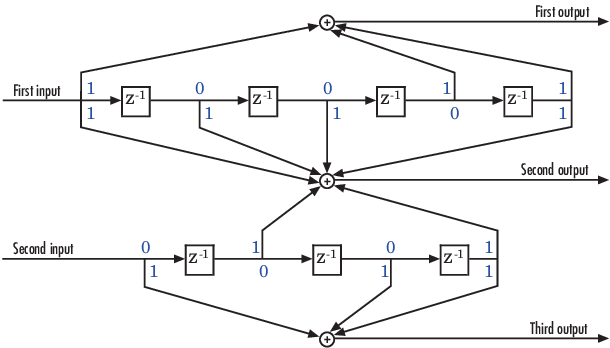
Determining Coding Parameters. The convenc and vitdec functions
can implement this code if their parameters have the appropriate
values.
The encoder’s constraint length is a vector of length 2 because the
encoder has two inputs. The elements of this vector indicate the number of
bits stored in each shift register, including the current input bits.
Counting memory spaces in each shift register in the diagram and adding one
for the current inputs leads to a constraint length of [5 4].
To determine the code generator parameter as a 2-by-3 matrix of octal
numbers, use the element in the ith row and jth column to indicate how the
ith input contributes to the jth output. For example, to compute the element
in the second row and third column, the leftmost and two rightmost elements
in the second shift register of the diagram feed into the sum that forms the
third output. Capture this information as the binary number 1011, which is
equivalent to the octal number 13. The full value of the code generator
matrix is [23 35 0; 0 5 13].
To use the constraint length and code generator parameters in the
convenc and vitdec functions,
use the poly2trellis function to convert those
parameters into a trellis structure. The command to do this is below.
trel = poly2trellis([5 4],[23 35 0;0 5 13]); % Define trellis.
Using the Encoder. Below is a script that uses this encoder.
len = 1000; msg = randi([0 1],2*len,1); % Random binary message of 2-bit symbols trel = poly2trellis([5 4],[23 35 0;0 5 13]); % Trellis % Create a ConvolutionalEncoder System object hConvEnc = comm.ConvolutionalEncoder(trel); % Create a ViterbiDecoder System object hVitDec = comm.ViterbiDecoder(trel, 'InputFormat', 'hard', ... 'TracebackDepth', 34, 'TerminationMethod', 'Continuous'); % Create a ErrorRate Calculator System object. Since each symbol represents % two bits, the receive delay for this object is twice the traceback length % of the viterbi decoder. hErrorCalc = comm.ErrorRate('ReceiveDelay', 68); ber = zeros(3,1); % Store BER values code = step(hConvEnc,msg); % Encode the message. ncode = rem(code + randerr(3*len,1,[0 1;.96 .04]),2); % Add noise. decoded = step(hVitDec, ncode); % Decode. ber = step(hErrorCalc, msg, decoded);
convenc accepts a vector containing 2-bit symbols and
produces a vector containing 3-bit symbols, while
vitdec does the opposite. Also notice that
biterr ignores the first 68 elements of
decoded. That is, the decoding delay is 68, which is
the number of bits per symbol (2) of the recovered message times the
traceback depth value (34) in the vitdec function. The
first 68 elements of decoded are 0s, while subsequent
elements represent the decoded messages.
Design a Rate 2/3 Feedforward Encoder Using Simulink
This example uses the rate 2/3 feedforward convolutional encoder depicted in
the following figure. The description explains how to determine the coding
blocks’ parameters from a schematic of a rate 2/3 feedforward encoder. This
example also illustrates the use of the Error Rate Calculation block with a
receive delay.
How to Determine Coding Parameters. The Convolutional Encoder and Viterbi Decoder blocks can
implement this code if their parameters have the appropriate values.
The encoder’s constraint length is a vector of length 2 since the encoder
has two inputs. The elements of this vector indicate the number of bits
stored in each shift register, including the current input bits. Counting
memory spaces in each shift register in the diagram and adding one for the
current inputs leads to a constraint length of [5 4].
To determine the code generator parameter as a 2-by-3 matrix of octal
numbers, use the element in the ith row and jth column to indicate how the
ith input contributes to the jth output. For example, to compute the element
in the second row and third column, notice that the leftmost and two
rightmost elements in the second shift register of the diagram feed into the
sum that forms the third output. Capture this information as the binary
number 1011, which is equivalent to the octal number 13. The full value of
the code generator matrix is [27 33 0; 0 5 13].
To use the constraint length and code generator parameters in the
Convolutional Encoder and Viterbi Decoder blocks, use the
poly2trellis function to convert those parameters
into a trellis structure.
How to Simulate the Encoder. The following model simulates this encoder.
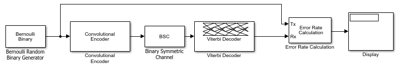
To open the completed model, enter doc_convcoding at
the MATLAB command line. To build the model, gather and configure these
blocks:
-
Bernoulli Binary
Generator, in the Comm Sources library-
Set Probability of a zero to
.5. -
Set Initial seed to any positive
integer scalar, preferably the output of therandn
function. -
Set Sample time to
.5. -
Check the Frame-based outputs check
box. -
Set Samples per frame to
2.
-
-
Convolutional
Encoder-
Set Trellis structure to
poly2trellis([5 4],[23 35 0; 0 5.
13])
-
-
Binary Symmetric Channel,
in the Channels library-
Set Error probability to
0.02. -
Set Initial seed to any positive
integer scalar, preferably the output of therandn
function. -
Clear the Output error vector check
box.
-
-
Viterbi Decoder
-
Set Trellis structure to
poly2trellis([5 4],[23 35 0; 0 5.
13]) -
Set Decision type to
Hard decision.
-
-
Error Rate Calculation,
in the Comm Sinks library-
Set Receive delay to
68. -
Set Output data to
Port. -
Check the Stop simulation check
box. -
Set Target number of errors to
100.
-
-
Display (Simulink), in the
Simulink Sinks library-
Drag the bottom edge of the icon to make the display big
enough for three entries.
-
Connect the blocks as shown in the preceding figure. On the
tab, in the
section, set Stop
time to inf. The
section appears on multiple
tabs.
Notes on the Model. You can display the matrix size of signals in your model. On the
tab, expand . In the
section, select .
The encoder accepts a 2-by-1 column vector and produces a 3-by-1 column
vector, while the decoder does the opposite. The Samples per
frame parameter in the Bernoulli Binary Generator block is 2
because the block must generate a message word of length 2.
The Receive delay parameter in the Error Rate
Calculation block is 68, which is the vector length (2) of the recovered
message times the Traceback depth value (34) in the
Viterbi Decoder block. If you examine the transmitted and received signals
as matrices in the MATLAB workspace, you see that the first 34 rows of the recovered
message consist of zeros, while subsequent rows are the decoded messages.
Thus the delay in the received signal is 34 vectors of length 2, or 68
samples.
Running the model produces display output consisting of three numbers: the
error rate, the total number of errors, and the total number of comparisons
that the Error Rate Calculation block makes during the simulation. (The
first two numbers vary depending on your Initial seed
values in the Bernoulli Binary Generator and Binary Symmetric Channel
blocks.) The simulation stops after 100 errors occur, because
Target number of errors is set to
100 in the Error Rate Calculation block. The error
rate is much less than 0.02, the Error
probability in the Binary Symmetric Channel block.
Puncture a Convolutional Code Using MATLAB
This example processes a punctured convolutional code. It begins by generating
30,000 random bits and encoding them using a rate-3/4 convolutional encoder with
a puncture pattern of [1 1 1 0 0 1]. The resulting vector contains 40,000 bits,
which are mapped to values of -1 and 1 for transmission. The punctured code,
punctcode, passes through an additive white Gaussian
noise channel. Then vitdec decodes the noisy vector using
the 'unquant' decision type.
Finally, the example computes the bit error rate and the number of bit
errors.
len = 30000; msg = randi([0 1], len, 1); % Random data t = poly2trellis(7, [133 171]); % Define trellis. % Create a ConvolutionalEncoder System object hConvEnc = comm.ConvolutionalEncoder(t, ... 'PuncturePatternSource', 'Property', ... 'PuncturePattern', [1;1;1;0;0;1]); % Create an AWGNChannel System object. hChan = comm.AWGNChannel('NoiseMethod', 'Signal to noise ratio (SNR)',... 'SNR', 3); % Create a ViterbiDecoder System object hVitDec = comm.ViterbiDecoder(t, 'InputFormat', 'Unquantized', ... 'TracebackDepth', 96, 'TerminationMethod', 'Truncated', ... 'PuncturePatternSource', 'Property', ... 'PuncturePattern', [1;1;1;0;0;1]); % Create a ErrorRate Calculator System object. hErrorCalc = comm.ErrorRate; berP = zeros(3,1); berPE = berP; % Store BER values punctcode = step(hConvEnc,msg); % Length is (2*len)*2/3. tcode = 1-2*punctcode; % Map "0" bit to 1 and "1" bit to -1 hChan.SignalPower = (tcode'*tcode)/length(tcode); ncode = step(hChan,tcode); % Add noise. % Decode the punctured code decoded = step(hVitDec,ncode); % Decode. berP = step(hErrorCalc, msg, decoded);% Bit error rate % Erase the least reliable 100 symbols, then decode release(hVitDec); reset(hErrorCalc) hVitDec.ErasuresInputPort = true; [dummy idx] = sort(abs(ncode)); erasures = zeros(size(ncode)); erasures(idx(1:100)) = 1; decoded = step(hVitDec,ncode, erasures); % Decode. berPE = step(hErrorCalc, msg, decoded);% Bit error rate fprintf('Number of errors with puncturing: %dn', berP(2)) fprintf('Number of errors with puncturing and erasures: %dn', berPE(2))
Implement a Systematic Encoder with Feedback Using Simulink
This section explains how to use the Convolutional Encoder block to implement
a systematic encoder with feedback. A code is systematic if
the actual message words appear as part of the codewords. The following diagram
shows an example of a systematic encoder.
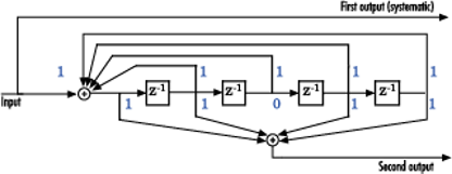
To implement this encoder, set the Trellis structure
parameter in the Convolutional Encoder block to poly2trellis(5, [37. This setting corresponds to
33], 37)
-
Constraint length:
5 -
Generator polynomial pair:
[37 33] -
Feedback polynomial:
37
The feedback polynomial is represented by the binary vector [1 1 1 1 1],
corresponding to the upper row of binary digits. These digits indicate
connections from the outputs of the registers to the adder. The initial 1
corresponds to the input bit. The octal representation of the binary number
11111 is 37.
To implement a systematic code, set the first generator polynomial to be the
same as the feedback polynomial in the Trellis structure
parameter of the Convolutional Encoder block. In this example, both polynomials
have the octal representation 37.
The second generator polynomial is represented by the binary vector [1 1 0
1 1], corresponding to the lower row of binary digits. The octal number
corresponding to the binary number 11011 is 33.
For more information on setting the mask parameters for the Convolutional
Encoder block, see Polynomial
Description of a Convolutional Code.
Soft-Decision Decoding
This example creates a rate 1/2 convolutional code. It uses a quantizer and
the Viterbi Decoder block to perform soft-decision decoding. This description
covers these topics:
-
Overview of the Simulation
-
Defining the Convolutional Code
-
Mapping the Received Data
-
Decoding the Convolutional Code
-
Delay in Received Data
-
Comparing Simulation Results with Theoretical Results
Overview of the Simulation. The model is in the following figure. To open the model, enter
doc_softdecision at the MATLAB command line. The simulation creates a random binary message
signal, encodes the message into a convolutional code, modulates the code
using the binary phase shift keying (BPSK) technique, and adds white
Gaussian noise to the modulated data in order to simulate a noisy channel.
Then, the simulation prepares the received data for the decoding block and
decodes. Finally, the simulation compares the decoded information with the
original message signal in order to compute the bit error rate. The
Convolutional encoder is configured as a rate 1/2 encoder. For every 2 bits,
the encoder adds another 2 redundant bits. To accommodate this, and add the
correct amount of noise, the Eb/No (dB) parameter of
the AWGN block is in effect halved by subtracting 10*log10(2). The
simulation ends after processing 100 bit errors or
107 message bits, whichever comes
first.
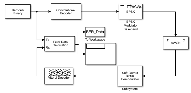
Defining the Convolutional Code. The feedforward convolutional encoder in this example is depicted
below.
The encoder’s constraint length is a scalar since the encoder has one
input. The value of the constraint length is the number of bits stored in
the shift register, including the current input. There are six memory
registers, and the current input is one bit. Thus the constraint length of
the code is 7.
The code generator is a 1-by-2 matrix of octal numbers because the encoder
has one input and two outputs. The first element in the matrix indicates
which input values contribute to the first output, and the second element in
the matrix indicates which input values contribute to the second
output.
For example, the first output in the encoder diagram is the modulo-2 sum
of the rightmost and the four leftmost elements in the diagram’s array of
input values. The seven-digit binary number 1111001 captures this
information, and is equivalent to the octal number 171. The octal number 171
thus becomes the first entry of the code generator matrix. Here, each
triplet of bits uses the leftmost bit as the most significant bit. The
second output corresponds to the binary number 1011011, which is equivalent
to the octal number 133. The code generator is therefore
[171 133].
The Trellis structure parameter in the Convolutional
Encoder block tells the block which code to use when processing data. In
this case, the poly2trellis function, in
Communications Toolbox, converts the constraint length and the pair of octal numbers
into a valid trellis structure.
While the message data entering the Convolutional Encoder block is a
scalar bit stream, the encoded data leaving the block is a stream of binary
vectors of length 2.
Mapping the Received Data. The received data, that is, the output of the AWGN Channel block, consists
of complex numbers that are close to -1 and 1. In order to reconstruct the
original binary message, the receiver part of the model must decode the
convolutional code. The Viterbi Decoder block in this model expects its
input data to be integers between 0 and 7. The demodulator, a custom
subsystem in this model, transforms the received data into a format that the
Viterbi Decoder block can interpret properly. More specifically, the
demodulator subsystem
-
Converts the received data signal to a real signal by removing its
imaginary part. It is reasonable to assume that the imaginary part
of the received data does not contain essential information, because
the imaginary part of the transmitted data is zero (ignoring small
roundoff errors) and because the channel noise is not very
powerful. -
Normalizes the received data by dividing by the standard deviation
of the noise estimate and then multiplying by -1. -
Quantizes the normalized data using three bits.
The combination of this mapping and the Viterbi Decoder block’s decision
mapping reverses the BPSK modulation that the BPSK Modulator Baseband block
performs on the transmitting side of this model. To examine the demodulator
subsystem in more detail, double-click the icon labeled Soft-Output BPSK
Demodulator.
Decoding the Convolutional Code. After the received data is properly mapped to length-2 vectors of 3-bit
decision values, the Viterbi Decoder block decodes it. The block uses a
soft-decision algorithm with 23 different input
values because the Decision type parameter is
Soft Decision and the Number of
soft decision bits parameter is 3.
Soft-Decision Interpretation of
Data
When the Decision type parameter is set to
Soft Decision, the Viterbi Decoder block
requires input values between 0 and 2b-1, where
b is the Number of soft decision
bits parameter. The block interprets 0 as the most confident
decision that the codeword bit is a 0 and interprets
2b-1 as the most confident decision that the
codeword bit is a 1. The values in between these extremes represent less
confident decisions. The following table lists the interpretations of the
eight possible input values for this example.
| Decision Value | Interpretation |
|---|---|
| 0 | Most confident 0 |
| 1 | Second most confident 0 |
| 2 | Third most confident 0 |
| 3 | Least confident 0 |
| 4 | Least confident 1 |
| 5 | Third most confident 1 |
| 6 | Second most confident 1 |
| 7 | Most confident 1 |
Traceback and Decoding Delay
The Traceback depth parameter in the Viterbi Decoder
block represents the length of the decoding delay. Typical values for a
traceback depth are about five or six times the constraint length, which
would be 35 or 42 in this example. However, some hardware implementations
offer options of 48 and 96. This example chooses 48 because that is closer
to the targets (35 and 42) than 96 is.
Delay in Received Data. The Receive delay parameter of the Error Rate Calculation block is
nonzero because a given message bit and its corresponding recovered bit are
separated in time by a nonzero amount of simulation time. The
Receive delay parameter tells the block which
elements of its input signals to compare when checking for errors.
In this case, the Receive delay value is equal to the Traceback depth
value (48).
Comparing Simulation Results with Theoretical Results. This section describes how to compare the bit error rate in this
simulation with the bit error rate that would theoretically result from
unquantized decoding. The process includes a few steps, described in these
sections:
Computing Theoretical Bounds for the Bit Error
Rate
To calculate theoretical bounds for the bit error rate
Pb of the convolutional code
in this model, you can use this estimate based on unquantized-decision
decoding:
In this estimate, cd is the
sum of bit errors for error events of distance d, and
f is the free distance of the code. The quantity
Pd is the pairwise error
probability, given by
where R is the code rate of 1/2, and erfc is the MATLAB complementary error function, defined by
Values for the coefficients cd
and the free distance f are in published articles such
as «Convolutional Codes with Optimum Distance Spectrum» [3]. The free distance for this code is
f = 10.
The following commands calculate the values of
Pb for
Eb/N0
values in the range from 1 to 4, in increments of 0.5:
EbNoVec = [1:0.5:4.0];
R = 1/2;
% Errs is the vector of sums of bit errors for
% error events at distance d, for d from 10 to 29.
Errs = [36 0 211 0 1404 0 11633 0 77433 0 502690 0,...
        3322763 0 21292910 0 134365911 0 843425871 0];
% P is the matrix of pairwise error probilities, for
% Eb/No values in EbNoVec and d from 10 to 29.
P = zeros(20,7); % Initialize.
for d = 10:29
   P(d-9,:) = (1/2)*erfc(sqrt(d*R*10.^(EbNoVec/10)));
end
% Bounds is the vector of upper bounds for the bit error
% rate, for Eb/No values in EbNoVec.
Bounds = Errs*P;
Simulating Multiple Times to Collect Bit Error
Rates
You can efficiently vary the simulation parameters by using the sim (Simulink) function to run the
simulation from the MATLAB command line. For example, the following code calculates the
bit error rate at bit energy-to-noise ratios ranging from 1 dB to 4 dB, in
increments of 0.5 dB. It collects all bit error rates from these simulations
in the matrix BERVec. It also plots the bit error rates
in a figure window along with the theoretical bounds computed in the
preceding code fragment.
Note
To open the model, enter doc_softdecision at the
MATLAB command line. Then execute these commands, which might
take a few minutes.
Note
The estimate for Pb
assumes that the decoder uses unquantized data, that is, an infinitely
fine quantization. By contrast, the simulation in this example uses
8-level (3-bit) quantization. Because of this quantization, the
simulated bit error rate is not quite as low as the bound when the
signal-to-noise ratio is high.
The plot of bit error rate against signal-to-noise ratio follows. The
locations of your actual BER points might vary because the simulation
involves random numbers.
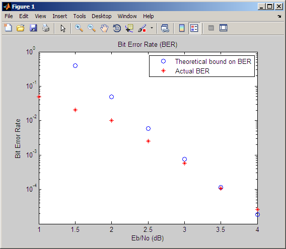
Tailbiting Encoding Using Feedback Encoders
This example demonstrates Tailbiting encoding using feedback encoders. For
feedback encoders, the ending state depends on the entire block of data. To
accomplish tailbiting, you must calculate for a given information vector (of N
bits), the initial state, that leads to the same ending state after the block of
data is encoded.
This is achieved in two steps:
-
The first step is to determine the zero-state response for a given
block of data. The encoder starts in the all-zeros state. The whole
block of data is input and the output bits are ignored. After N
bits, the encoder is in a state
XN
[zs]. From this state, we calculate the
corresponding initial state
X0 and initialize the
encoder with X0. -
The second step is the actual encoding. The encoder starts with
the initial state X0, the
data block is input and a valid codeword is output which conforms to
the same state boundary condition.
Refer to [8] for a theoretical calculation of the initial state
X0 from
XN
[zs] using state-space formulation. This is a
one-time calculation which depends on the block length and in practice could be
implemented as a look-up table. Here we determine this mapping table by
simulating all possible entries for a chosen trellis and block length.
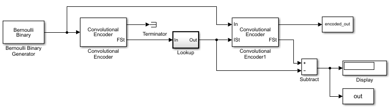
To open the model, enter doc_mtailbiting_wfeedback at the
MATLAB command line.
function mapStValues = getMapping(blkLen, trellis)
% The function returns the mapping value for the given block
length and trellis to be used for determining the initial
state from the zero-state response.

% All possible combinations of the mappings
mapStValuesTab = perms(0:trellis.numStates-1);

% Loop over all the combinations of the mapping entries:
for i = 1:length(mapStValuesTab)
mapStValues = mapStValuesTab(i,:);

% Model parameterized for the Block length
sim('mtailbiting_wfeedback');

% Check the boundary condition for each run
% if ending and starting states match, choose that mapping set
if unique(out)==0
        return
    end
end
Selecting the returned mapStValues for the Table
data parameter of the Direct Lookup Table block in the Lookup subsystem will perform tailbiting
(n-D)
encoding for the chosen block length and trellis.
Selected Bibliography for Convolutional Coding
[1] Clark, George C. Jr., and J. Bibb Cain,
Error-Correction Coding for Digital
Communications, New York, Plenum Press, 1981.
[2] Gitlin, Richard D., Jeremiah F. Hayes, and Stephen
B. Weinstein, Data Communications Principles, New
York, Plenum Press, 1992.
[3] Frenger, P., P. Orten, and T. Ottosson. “Convolutional Codes with Optimum Distance Spectrum.” IEEE Communications Letters 3, no. 11 (November 1999): 317–19. https://doi.org/10.1109/4234.803468.
Linear Block Codes
-
Represent Words for Linear Block Codes
-
Configure Parameters for Linear Block Codes
-
Create and Decode Linear Block Codes
Represent Words for Linear Block Codes
The cyclic, Hamming, and generic linear block code functionality in this
product offers you multiple ways to organize bits in messages or codewords.
These topics explain the available formats:
-
Use MATLAB to Create Messages and Codewords in Binary Vector
Format -
Use MATLAB to Create Messages and Codewords in Binary Matrix
Format -
Use MATLAB to Create Messages and Codewords in Decimal Vector
Format
To learn how to represent words for BCH or Reed-Solomon codes, see Represent Words for BCH Codes or Represent Words for Reed-Solomon Codes.
Use MATLAB to Create Messages and Codewords in Binary Vector
Format. Your messages and codewords can take the form of vectors containing 0s and
1s. For example, messages and codes might look like msg
and code in the lines below.
n = 6; k = 4; % Set codeword length and message length
% for a [6,4] code.
msg = [1 0 0 1 1 0 1 0 1 0 1 1]'; % Message is a binary column.
code = encode(msg,n,k,'cyclic'); % Code will be a binary column.
msg'
code'
The output is below.
ans =

  Columns 1 through 5

      1            0            0            1            1

  Columns 6 through 10

      0            1            0            1            0

  Columns 11 through 12

      1            1


ans =

  Columns 1 through 5

      1            1            1            0            0

  Columns 6 through 10

      1            0            0            1            0

  Columns 11 through 15

      1            0            0            1            1

  Columns 16 through 18

      0            1            1
In this example, msg consists of 12 entries, which are
interpreted as three 4-digit (because k = 4)
messages. The resulting vector code comprises three
6-digit (because n = 6) codewords, which are
concatenated to form a vector of length 18. The parity bits are at the
beginning of each codeword.
Use MATLAB to Create Messages and Codewords in Binary Matrix
Format. You can organize coding information so as to emphasize the grouping of
digits into messages and codewords. If you use this approach, each message
or codeword occupies a row in a binary matrix. The example below illustrates
this approach by listing each 4-bit message on a distinct row in
msg and each 6-bit codeword on a distinct row in
code.
n = 6; k = 4; % Set codeword length and message length.
msg = [1 0 0 1; 1 0 1 0; 1 0 1 1]; % Message is a binary matrix.
code = encode(msg,n,k,'cyclic'); % Code will be a binary matrix.
msg
code
The output is below.
msg =

     1     0     0     1
     1     0     1     0
     1     0     1     1


code =

     1     1     1     0     0     1
     0     0     1     0     1     0
     0     1     1     0     1     1
Note
In the binary matrix format, the message matrix must have
k columns. The corresponding code matrix has
n columns. The parity bits are at the beginning
of each row.
Use MATLAB to Create Messages and Codewords in Decimal Vector
Format. Your messages and codewords can take the form of vectors containing
integers. Each element of the vector gives the decimal representation of the
bits in one message or one codeword.
Note
If 2^n or 2^k is very large, you
should use the default binary format instead of the decimal format. This
is because the function uses a binary format internally, while the
roundoff error associated with converting many bits to large decimal
numbers and back might be substantial.
Note
When you use the decimal vector format, encode
expects the leftmost bit to be the least
significant bit.
The syntax for the encode command must mention the
decimal format explicitly, as in the example below. Notice that
/decimal is appended to the fourth argument in the
encode command.
n = 6; k = 4; % Set codeword length and message length.
msg = [9;5;13]; % Message is a decimal column vector.
% Code will be a decimal vector.
code = encode(msg,n,k,'cyclic/decimal')
The output is below.
Note
The three examples above used cyclic coding. The formats for messages
and codes are similar for Hamming and generic linear block codes.
Configure Parameters for Linear Block Codes
This subsection describes the items that you might need in order to process
[n,k] cyclic, Hamming, and generic linear block codes. The table below lists the
items and the coding techniques for which they are most relevant.
Parameters Used in Block Coding Techniques
Generator Matrix. The process of encoding a message into an [n,k] linear block code is
determined by a k-by-n generator matrix G. Specifically, the 1-by-k message
vector v is encoded into the 1-by-n codeword vector vG. If G has the form
[Ik P] or
[P Ik], where P is some k-by-(n-k) matrix and
Ik is the k-by-k identity matrix, G is said to be
in standard form. (Some authors, e.g., Clark and Cain
[2], use the first standard form, while others, e.g., Lin and Costello [3], use the second.) Most functions in this toolbox assume that a generator
matrix is in standard form when you use it as an input argument.
Some examples of generator matrices are in the next section, Parity-Check Matrix.
Parity-Check Matrix. Decoding an [n,k] linear block code requires an (n-k)-by-n parity-check
matrix H. It satisfies
GHtr = 0 (mod
2), where Htr denotes the matrix transpose of H,
G is the code’s generator matrix, and this zero matrix is k-by-(n-k). If
G = [Ik P] then
H = [-Ptr In-k].
Most functions in this product assume that a parity-check matrix is in
standard form when you use it as an input argument.
The table below summarizes the standard forms of the generator and
parity-check matrices for an [n,k] binary linear block code.
| Type of Matrix |
Standard Form |
Dimensions |
|---|---|---|
| Generator | [Ik P] or [P Ik] |
k-by-n |
| Parity-check | [-P'In-k] or [In-k -P '] |
(n-k)-by-n |
Ik is the identity matrix of size k and the
' symbol indicates matrix transpose. (For
binary codes, the minus signs in the parity-check
form listed above are irrelevant; that is, -1 = 1 in the binary
field.)
Examples
In the command below, parmat is a parity-check matrix
and genmat is a generator matrix for a Hamming code in
which
[n,k] = [23-1, n-3] = [7,4].
genmat has the standard form
[P Ik].
[parmat,genmat] = hammgen(3)
parmat =

     1     0     0     1     0     1     1
     0     1     0     1     1     1     0
     0     0     1     0     1     1     1

genmat =

     1     1     0     1     0     0     0
     0     1     1     0     1     0     0
     1     1     1     0     0     1     0
     1     0     1     0     0     0     1
The next example finds parity-check and generator matrices for a [7,3]
cyclic code. The cyclpoly function is mentioned below
in Generator Polynomial.
genpoly = cyclpoly(7,3);
[parmat,genmat] = cyclgen(7,genpoly)
parmat =

     1     0     0     0     1     1     0
     0     1     0     0     0     1     1
     0     0     1     0     1     1     1
     0     0     0     1     1     0     1

genmat =

     1     0     1     1     1     0     0
     1     1     1     0     0     1     0
     0     1     1     1     0     0     1
The example below converts a generator matrix for a [5,3] linear block
code into the corresponding parity-check matrix.
genmat = [1 0 0 1 0; 0 1 0 1 1; 0 0 1 0 1];
parmat = gen2par(genmat)

parmat =

     1     1     0     1     0
     0     1     1     0     1
The same function gen2par can also convert a
parity-check matrix into a generator matrix.
Generator Polynomial. Cyclic codes have algebraic properties that allow a polynomial to
determine the coding process completely. This so-called generator
polynomial is a degree-(n-k) divisor of the polynomial
xn-1. Van Lint [5] explains how a generator polynomial determines a cyclic code.
The cyclpoly function produces generator polynomials
for cyclic codes. cyclpoly represents a generator
polynomial using a row vector that lists the polynomial’s coefficients in
order of ascending powers of the variable. For example,
the command
genpoly = cyclpoly(7,3)

genpoly =

     1     0     1     1     1
finds that one valid generator polynomial for a [7,3] cyclic code is
1 + x2 + x3 + x4.
Use Decoding Table in MATLAB
A decoding table tells a decoder how to correct errors that might have corrupted the code during transmission. Hamming codes can correct any single-symbol error in any codeword. Other codes can correct, or partially correct, errors that corrupt more than one symbol in a given codeword.
This toolbox represents a decoding table as a matrix with n columns and 2^(n—k) rows. Each row gives a correction vector for one received codeword vector. A Hamming decoding table has n+1 rows. The syndtable function generates a decoding table for a given parity-check matrix.
This example uses a Hamming decoding table to correct an error in a received message. The hammgen function produces the parity-check matrix and the syndtable function produces the decoding table. To determine the syndrome, the transpose of the parity-check matrix is multiplied on the left by the received codeword. The decoding table helps determine the correction vector. The corrected codeword is the sum (modulo 2) of the correction vector and the received codeword.
Set parameters for a [7,4] Hamming code.
m = 3;
n = 2^m-1;
k = n-m;
Produce a parity-check matrix and decoding table.
parmat = hammgen(m);
trt = syndtable(parmat);
Specify a vector of received data.
Calculate the syndrome, and then display the decimal and binary value for the syndrome.
syndrome = rem(recd * parmat',2);
syndrome_int = bit2int(syndrome',m); % Convert to decimal.
disp(['Syndrome = ',num2str(syndrome_int),...
      ' (decimal), ',num2str(syndrome),' (binary)'])
Syndrome = 3 (decimal), 0 1 1 (binary)
Determine the correction vector by using the decoding table and syndrome, and then compute the corrected codeword by using the correction vector.
corrvect = trt(1+syndrome_int,:)
corrvect = 1×7

     0     0     0     0     1     0     0
correctedcode = rem(corrvect+recd,2)
correctedcode = 1×7

     1     0     0     1     0     1     1
Create and Decode Linear Block Codes
The functions for encoding and decoding cyclic, Hamming, and generic linear
block codes are encode and decode.
This section discusses how to use these functions to create and decode generic linear block
codes, cyclic codes, and
Hamming
codes.
Generic Linear Block Codes. Encoding a message using a generic linear block code requires a generator
matrix. If you have defined variables msg,
n, k, and
genmat, either of the commands
code = encode(msg,n,k,'linear',genmat);
code = encode(msg,n,k,'linear/decimal',genmat);
encodes the information in msg using the
[n,k] code that the generator
matrix genmat determines. The /decimal
option, suitable when 2^n and 2^k are
not very large, indicates that msg contains nonnegative
decimal integers rather than their binary representations. See Represent Words for Linear Block Codes or the reference page
for encode for a description of
the formats of msg and code.
Decoding the code requires the generator matrix and possibly a decoding
table. If you have defined variables code,
n, k, genmat,
and possibly also trt, then the commands
newmsg = decode(code,n,k,'linear',genmat);
newmsg = decode(code,n,k,'linear/decimal',genmat);
newmsg = decode(code,n,k,'linear',genmat,trt);
newmsg = decode(code,n,k,'linear/decimal',genmat,trt);
decode the information in code, using the
[n,k] code that the generator
matrix genmat determines. decode
also corrects errors according to instructions in the decoding table that
trt represents.
Example: Generic Linear Block
Coding
The example below encodes a message, artificially adds some noise, decodes
the noisy code, and keeps track of errors that the decoder detects along the
way. Because the decoding table contains only zeros, the decoder does not
correct any errors.
n = 4; k = 2;
genmat = [[1 1; 1 0], eye(2)]; % Generator matrix
msg = [0 1; 0 0; 1 0]; % Three messages, two bits each
% Create three codewords, four bits each.
code = encode(msg,n,k,'linear',genmat);
noisycode = rem(code + randerr(3,4,[0 1;.7 .3]),2); % Add noise.
trt = zeros(2^(n-k),n);  % No correction of errors
% Decode, keeping track of all detected errors.
[newmsg,err] = decode(noisycode,n,k,'linear',genmat,trt);
err_words = find(err~=0) % Find out which words had errors.
The output indicates that errors occurred in the first and second words.
Your results might vary because this example uses random numbers as
errors.
Cyclic Codes. A cyclic code is a linear block code with the property that cyclic shifts
of a codeword (expressed as a series of bits) are also codewords. An
alternative characterization of cyclic codes is based on its generator
polynomial, as mentioned in Generator Polynomial and discussed in [5].
Encoding a message using a cyclic code requires a generator polynomial. If
you have defined variables msg, n,
k, and genpoly, then either of the
commands
code = encode(msg,n,k,'cyclic',genpoly);
code = encode(msg,n,k,'cyclic/decimal',genpoly);
encodes the information in msg using the
[n,k] code determined by the
generator polynomial genpoly. genpoly
is an optional argument for encode. The default
generator polynomial is cyclpoly(n,k). The
/decimal option, suitable when 2^n
and 2^k are not very large, indicates that
msg contains nonnegative decimal integers rather than
their binary representations. See Represent Words for Linear Block Codes or the reference page
for encode for a description of
the formats of msg and code.
Decoding the code requires the generator polynomial and possibly a
decoding table. If you have defined variables code,
n, k, genpoly,
and trt, then the commands
newmsg = decode(code,n,k,'cyclic',genpoly);
newmsg = decode(code,n,k,'cyclic/decimal',genpoly);
newmsg = decode(code,n,k,'cyclic',genpoly,trt);
newmsg = decode(code,n,k,'cyclic/decimal',genpoly,trt);
decode the information in code, using the
[n,k] code that the generator
matrix genmat determines. decode
also corrects errors according to instructions in the decoding table that
trt represents. genpoly is an
optional argument in the first two syntaxes above. The default generator
polynomial is cyclpoly(n,k).
Example
You can modify the example in Generic Linear Block Codes
so that it uses the cyclic coding technique, instead of the linear block
code with the generator matrix genmat. Make the changes
listed below:
-
Replace the second line by
genpoly = [1 0 1]; % generator poly is 1 + x^2 -
In the fifth and ninth lines (
encodeand
decodecommands), replace
genmatbygenpolyand
replace'linear'by
'cyclic'.
Another example of encoding and decoding a cyclic code is on the reference
page for encode.
Hamming Codes. The reference pages for encode and decode contain examples of
encoding and decoding Hamming codes. Also, the section Use Decoding Table in MATLAB illustrates error
correction in a Hamming code.
Hamming Codes
-
Create a Hamming Code in Binary Format Using Simulink
-
Reduce the Error Rate Using a Hamming Code
Create a Hamming Code in Binary Format Using Simulink
This example shows very simply how to use an encoder and decoder. It
illustrates the appropriate vector lengths of the code and message signals for
the coding blocks. Because the Error Rate Calculation block accepts
only scalars or frame-based column vectors as the transmitted and received
signals, this example uses frame-based column vectors throughout. (It thus
avoids having to change signal attributes using a block such as Convert 1-D to 2-D.)

Open this model by entering doc_hamming at the
MATLAB command line. To build the model, gather and configure these
blocks:
-
Bernoulli Binary Generator, in
the Comm Sources library-
Set Probability of a zero to
.5. -
Set Initial seed to any positive integer
scalar, preferably the output of therandn
function. -
Check the Frame-based outputs check
box. -
Set Samples per frame to
4.
-
-
Hamming Encoder, with default
parameter values -
Hamming Decoder, with default
parameter values -
Error Rate Calculation, in
the Comm Sinks library, with default parameter values
Connect the blocks as in the preceding figure. You can display the vector
length of signals in your model. On the tab,
expand . In the
section, select . After updating the diagram, if necessary, press
Ctrl+D to compile the model and check error statistics.
The connector lines show relevant signal attributes. The connector lines are
double lines to indicate frame-based signals, and the annotations next to the
lines show that the signals are column vectors of appropriate sizes.
Reduce the Error Rate Using a Hamming Code
This section describes how to reduce the error rate by adding an
error-correcting code. This figure shows model that uses a Hamming code.

To open a complete version of the model, enter doc_hamming
at the MATLAB prompt.
Building the Hamming Code Model
You can build the Hamming code model by following these steps:
-
Type
doc_channelat the MATLAB command line to open the channel noise model.
Then save the model as
my_hammingin the folder where you keep your
work files. -
From the Simulink Library Browser drag the Hamming Encoder and
Hamming Decoder blocks
from the Error Detection and Correction/Block sublibrary into the
model window. -
Click the right border of the model and drag it to the right to
widen the model window. -
Move the Binary Symmetric Channel,
Error Rate Calculation,
and Display (Simulink) blocks to
the right by clicking and dragging. -
Create enough space between the Bernoulli Binary Generator
and Binary Symmetric Channel
blocks to fit the Hamming Encoder between
them. -
Click and drag the Hamming Encoder block on top of
the line between the Bernoulli Binary Generator
block and the Binary Symmetric Channel block, to the
right of the branch point, as shown in the following figure. Then
release the mouse button. The Hamming Encoder block should
automatically connect to the line from the Bernoulli Binary
Generator block to the Binary Symmetric
Channel block. -
Move blocks again to create enough space between the Binary Symmetric Channel
and the Error Rate Calculation
blocks to fit the Hamming Decoder between
them. -
Click and drag the Hamming Decoder block on top of
the line between the Binary Symmetric Channel block
and the Error Rate Calculation block.

The model should now resemble this figure.
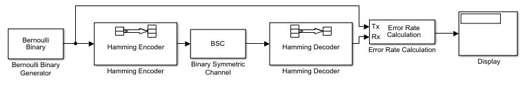
Using the Hamming Encoder and Decoder
Blocks
The Hamming Encoder block encodes the data before it is sent
through the channel. The default code is the [7,4] Hamming code, which encodes
message words of length 4 into codewords of length 7. As a result, the block
converts frames of size 4 into frames of size 7. The code can correct one error
in each transmitted codeword.
For an [n,k] code, the input to the Hamming Encoder block must consist of
vectors of size k. In this example, k = 4.
The Hamming Decoder block decodes the data after it is sent
through the channel. If at most one error is created in a codeword by the
channel, the block decodes the word correctly. However, if more than one error
occurs, the Hamming Decoder block might decode
incorrectly.
To learn more about block coding features, see Block Codes.
Setting Parameters in the Hamming Code
Model
Double-click the Bernoulli Binary Generator block and make the
following changes to the parameter settings in the block’s dialog box, as shown
in the following figure:
-
Set Samples per frame to
4. This converts the output of the block into
frames of size 4, in order to meet the input requirement of the
Hamming Encoder Block. See Sample-Based and Frame-Based Processing for more
information about frames.Note
Many blocks, such as the Hamming Encoder block,
require their input to be a vector of a specific size. If you
connect a source block, such as the Bernoulli Binary
Generator block, to one of these blocks, set
Samples per frame to the required
value. For this model the Samples per frame
parameter of the Bernoulli Binary Generator block
must be a multiple of the Message Length K
parameter of the Hamming Encoder block.
Labeling the Display Block
You can change the label that appears below a block to make it more
informative. For example, to change the label below the Display block to
'Error Rate Display', first select the label with the
mouse. This causes a box to appear around the text. Enter the changes to the
text in the box.
Running the Hamming Code Model
To run the model, select >
. The model terminates after 100 errors occur.
The error rate, displayed in the top window of the Display block, is
approximately .001. You get slightly different results if you change the
Initial seed parameters in the model or run a
simulation for a different length of time.
You expect an error rate of approximately .001 for the following reason: The
probability of two or more errors occurring in a codeword of length 7 is
1 – (0.99)7 –
7(0.99)6(0.01) = 0.002
If the codewords with two or more errors are decoded randomly, you expect
about half the bits in the decoded message words to be incorrect. This indicates
that .001 is a reasonable value for the bit error rate.
To obtain a lower error rate for the same probability of error, try using a
Hamming code with larger parameters. To do this, change the parameters
Codeword length and Message length
in the Hamming Encoder and Hamming
Decoder block dialog boxes. You also have to make the appropriate
changes to the parameters of the Bernoulli Binary Generator block
and the Binary Symmetric Channel block.
Displaying Frame Sizes
You can display the sizes of data frames in different parts in your model. On
the tab, expand . In the section,
select . The line leading out of the
Bernoulli Binary Generator block is labeled
[4x1], indicating that its output consists of column
vectors of size 4. Because the Hamming Encoder block uses a [7,4]
code, it converts frames of size 4 into frames of size 7, so its output is
labeled [7x1].
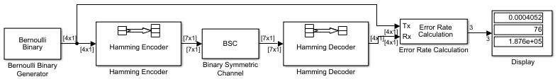
Adding a Scope to the Model
To display the channel errors produced by the Binary Symmetric
Channel block, add a Scope block to the model. This
is a good way to see whether your model is functioning correctly. The example
shown in the following figure shows where to insert the Scope
block into the model.
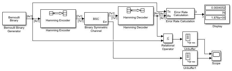
To build this model from the one shown in the figure Reduce the Error Rate Using a Hamming Code, follow these steps:
-
Drag the following blocks from the Simulink Library Browser into
the model window:-
Relational
Operator (Simulink) block, from the Simulink Logic and Bit
Operations library -
Scope (Simulink)
block, from the Simulink Sinks library -
Two copies of the Unbuffer block,
from the Buffers sublibrary of the Signal Management library
in DSP System Toolbox™
-
-
Double-click the Binary Symmetric Channel block to
open its dialog box, and select Output error
vector. This creates a second output port for the
block, which carries the error vector. -
Double-click the Scope block, under
> , set Number of input
ports to2. Select
Layout and highlight two blocks
vertically. Click OK. -
Connect the blocks as shown in the preceding figure.
Setting Parameters in the Expanded
Model
Make the following changes to the parameters for the blocks you added to the model.
-
Error Rate Calculation Block –
Double-click the Error Rate Calculation block and clear the box next
to Stop simulation in the block’s dialog
box. -
Scope Block – The Scope (Simulink) block
displays the channel errors and uncorrected errors. To configure the block,-
Double-click the Scope block, select
>
. -
Select the Time tab and set
Time span to
5000. -
Select the Logging tab and set
Limit data points to last to
30000. -
Click OK.
-
The scope should now appear as shown.

-
To configure the axes, follow these steps:
-
Right-click the vertical axis at the left side
of the upper scope. -
In the context menu, select
. -
Set Y-limits (Minimum) to
-1. -
Set Y-limits (Maximum) to
2, and click
OK. -
Repeat the same steps for the vertical axis of
the lower scope. -
Widen the scope window until it is roughly
three times as wide as it is high. You can do this
by clicking the right border of the window and
dragging the border to the right, while pressing
the left-mouse button.
-
-
-
Relational Operator – Set
Relational Operator to
~=in the block’s dialog box. The
Relational Operator block compares the transmitted signal, coming
from the Bernoulli Random Generator block, with the received signal,
coming from the Hamming Decoder block. The block outputs a 0 when
the two signals agree and a 1 when they disagree.
Observing Channel Errors with the
Scope
When you run the model, the scope displays the error data. At the end of each
5000 time steps, the scope appears as shown this figure. The scope then clears
the displayed data and displays the next 5000 data points.
The upper scope shows the channel errors generated by the Binary Symmetric Channel block. The
lower scope shows errors that are not corrected by channel coding.
Click the Stop button on the toolbar at the top of the
model window to stop the scope.
You can see individual errors by zooming in on the scope. First click the
middle magnifying glass button at the top left of the Scope
window. Then click one of the lines in the lower scope. This zooms in
horizontally on the line. Continue clicking the lines in the lower scope until
the horizontal scale is fine enough to detect individual errors. A typical
example of what you might see is shown in the figure below.
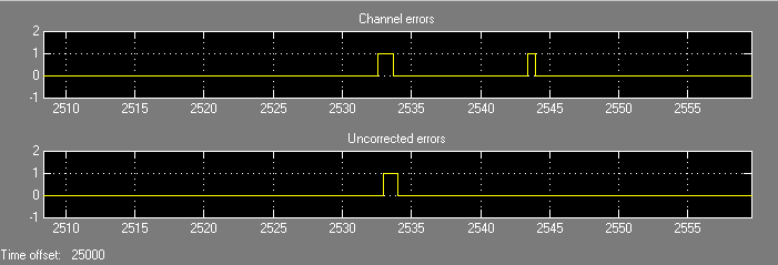
The wider rectangular pulse in the middle of the upper scope represents two
1s. These two errors, which occur in a single codeword, are not corrected. This
accounts for the uncorrected errors in the lower scope. The narrower rectangular
pulse to the right of the upper scope represents a single error, which is
corrected.
When you are done observing the errors, select
>
.
Export Data to MATLAB explains how to send the error data to the
MATLAB workspace for more detailed analysis.
BCH Codes
-
Represent Words for BCH Codes
-
Parameters for BCH Codes
-
Create and Decode BCH Codes
-
Algorithms for BCH and RS Errors-only Decoding
Represent Words for BCH Codes
A message for an [n,k] BCH code must be
a k-column binary Galois field array. The code that
corresponds to that message is an n-column binary Galois
field array. Each row of these Galois field arrays represents one word.
The example below illustrates how to represent words for a [15, 11] BCH
code.
msg = [1 0 0 1 0; 1 0 1 1 1]; % Messages in a Galois array
obj = comm.BCHEncoder;
c1 = step(obj, msg(1,:)');
c2 = step(obj, msg(2,:)');
cbch = [c1 c2].'
The output is
  Columns 1 through 5

      1            0            0            1            0
      1            0            1            1            1

  Columns 6 through 10

      0            0            1            1            1
      0            0            0            0            1

  Columns 11 through 15

      1            0            1            0            1
      0            1            0            0            1
Parameters for BCH Codes
BCH codes use special values of n and
k:
-
n, the codeword length, is an integer of the form
2m-1 for some integer
m > 2. -
k, the message length, is a positive integer less
thann. However, only some positive integers less
thannare valid choices fork.
See the BCH Encoder block reference
page for a list of some valid values ofk
corresponding to values ofnup to 511.
Create and Decode BCH Codes
The BCH Encoder and BCH Decoder System objects create and decode BCH codes, using the
data described in Represent Words for BCH Codes and Parameters for BCH Codes.
The topics are
-
Example: BCH Coding Syntaxes
-
Detect and Correct Errors in a BCH Code Using MATLAB
Example: BCH Coding Syntaxes. The example below illustrates how to encode and decode data using a
[15, 5] BCH code.
n = 15; k = 5; % Codeword length and message length
msg = randi([0 1],4*k,1); % Four random binary messages

% Simplest syntax for encoding
enc = comm.BCHEncoder(n,k);
dec = comm.BCHDecoder(n,k);
c1 = step(enc,msg); % BCH encoding
d1 = step(dec,c1); % BCH decoding

% Check that the decoding worked correctly.
chk = isequal(d1,msg)

% The following code shows how to perform the encoding and decoding
% operations if one chooses to prepend the parity symbols.

% Steps for converting encoded data with appended parity symbols
% to encoded data with prepended parity symbols
c11 = reshape(c1, n, []);
c12 = circshift(c11,n-k);
c1_prepend = c12(:); % BCH encoded data with prepended parity symbols

% Steps for converting encoded data with prepended parity symbols
% to encoded data with appended parity symbols prior to decoding
c21 = reshape(c1_prepend, n, []);
c22 = circshift(c21,k);
c1_append = c22(:); % BCH encoded data with appended parity symbols

% Check that the prepend-to-append conversion worked correctly.
d1_append = step(dec,c1_append);
chk = isequal(msg,d1_append)
The output is below.
Detect and Correct Errors in a BCH Code Using MATLAB. The following example illustrates the decoding results for a corrupted
code. The example encodes some data, introduces errors in each codeword, and
attempts to decode the noisy code using the BCH
Decoder
System object.
n = 15; k = 5; % Codeword length and message length
[gp,t] = bchgenpoly(n,k); % t is error-correction capability.
nw = 4; % Number of words to process
msgw = randi([0 1], nw*k, 1); % Random k-symbol messages
enc = comm.BCHEncoder(n,k,gp);
dec = comm.BCHDecoder(n,k,gp);
c = step(enc, msgw); % Encode the data.
noise = randerr(nw,n,t); % t errors per codeword
noisy = noise';
noisy = noisy(:);
cnoisy = mod(c + noisy,2); % Add noise to the code.
[dc, nerrs] = step(dec, cnoisy); % Decode cnoisy.

% Check that the decoding worked correctly.
chk2 = isequal(dc,msgw)
nerrs % Find out how many errors have been corrected.
Notice that the array of noise values contains binary values, and that the
addition operation c + noise takes place in the
Galois field GF(2) because c is a Galois field array in
GF(2).
The output from the example is below. The nonzero value of
ans indicates that the decoder was able to correct
the corrupted codewords and recover the original message. The values in the
vector nerrs indicate that the decoder corrected
t errors in each codeword.
Excessive Noise in BCH Codewords
In the previous example, the BCH Decoder
System object corrected all the errors. However, each BCH code has a finite
error-correction capability. To learn more about how the BCH Decoder
System object behaves when the noise is excessive, see the analogous
discussion for Reed-Solomon codes in Excessive Noise in Reed-Solomon Codewords.
Algorithms for BCH and RS Errors-only Decoding
Overview. The errors-only decoding algorithm used for BCH and RS codes can be
described by the following steps (sections 5.3.2, 5.4, and 5.6 in [2]).
-
Calculate the first 2t terms of the infinite
degree syndrome polynomial, S(z). -
If those 2t terms of S(z) are all equal to 0, then the code has no errors ,
no correction needs to be performed, and the decoding algorithm
ends. -
If one or more terms of S(z) are nonzero, calculate the error locator
polynomial, Λ(z), via the Berlekamp
algorithm. -
Calculate the error evaluator polynomial, Ω(z), via
-
Correct an error in the codeword according to
where eim is the error magnitude in the imth position in the codeword, m
is a value less than the error-correcting capability of the code, Ω(z) is the error magnitude polynomial,
Λ'(z) is the formal derivative [5] of the error locator polynomial, Λ(z), and α
is the primitive element of the Galois field of the code.
Further description of several of the steps is given in the following
sections.
Syndrome Calculation. For narrow-sense codes, the 2t terms of S(z) are calculated by evaluating the received codeword at
successive powers of α (the field’s primitive element) from 0 to
2t-1. In other words, if we assume one-based indexing
of codewords C(z) and the syndrome polynomial S(z), and that codewords are of the form [c1 c1 … cN], then each term Si of S(z) is given as
Error Locator Polynomial Calculation. The error locator polynomial, Λ(z), is found using the
Berlekamp algorithm. A complete description of this algorithm is found in
[2], but we summarize the algorithm as follows.
We define the following variables.
| Variable | Description |
|---|---|
| n | Iterator variable |
| k | Iterator variable |
| L | Length of the feedback register used to generate the first 2t terms of S(z) |
| D(z) | Correction polynomial |
| d | Discrepancy |
The following diagram shows the iterative procedure (i.e., the Berlekamp
algorithm) used to find Λ(z).
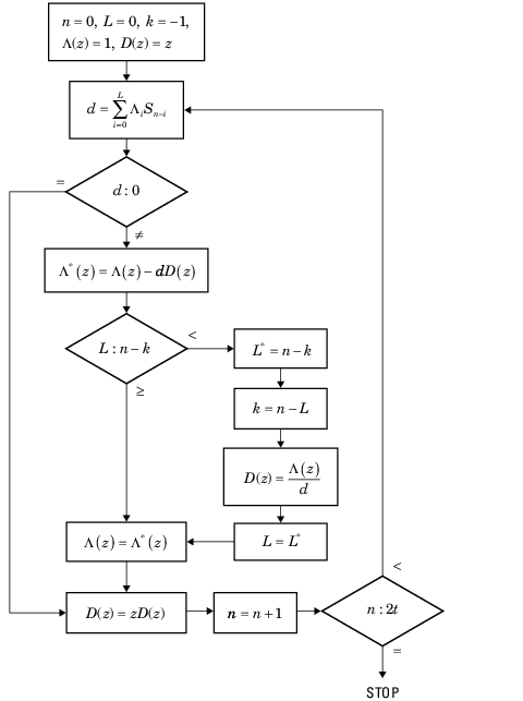
Error Evaluator Polynomial Calculation. The error evaluator polynomial, Ω(z), is simply the convolution of Λ(z) and S(z).
Reed-Solomon Codes
-
Represent Words for Reed-Solomon Codes
-
Parameters for Reed-Solomon Codes
-
Create and Decode Reed-Solomon Codes
-
Find a Generator Polynomial
-
Reed Solomon Examples with Shortening, Puncturing, and Erasures
Represent Words for Reed-Solomon Codes
This toolbox supports Reed-Solomon codes that use m-bit symbols instead of
bits. A message for an [n,k] Reed-Solomon
code must be a k-column Galois field array in the field
GF(2m). Each array entry must be an integer
between 0 and 2m-1. The code corresponding to that
message is an n-column Galois field array in
GF(2m). The codeword length n
must be between 3 and 2m-1.
The example below illustrates how to represent words for a [7,3] Reed-Solomon
code.
n = 7; k = 3; % Codeword length and message length
m = 3; % Number of bits in each symbol
msg = [1 6 4; 0 4 3]; % Message is a Galois array.
obj = comm.RSEncoder(n, k);
c1 = step(obj, msg(1,:)');
c2 = step(obj, msg(2,:)');
c = [c1 c2].'
The output is
C =

     1     6     4     4     3     6     3
     0     4     3     3     7     4     7
Parameters for Reed-Solomon Codes
This section describes several integers related to Reed-Solomon codes and
discusses how to find generator
polynomials.
Allowable Values of Integer Parameters. The table below summarizes the meanings and allowable values of some
positive integer quantities related to Reed-Solomon codes as supported in
this toolbox. The quantities n and k
are input parameters for Reed-Solomon functions in this toolbox.
| Symbol | Meaning | Value or Range |
|---|---|---|
| m | Number of bits per symbol | Integer between 3 and 16 |
n
|
Number of symbols per codeword | Integer between 3 and 2m-1 |
k |
Number of symbols per message | Positive integer less thann, such thatn-k is even |
| t | Error-correction capability of the code |
(n-k)/2 |
Generator Polynomial. The rsgenpoly function produces generator polynomials
for Reed-Solomon codes. rsgenpoly represents a
generator polynomial using a Galois row vector that lists the polynomial’s
coefficients in order of descending powers of the
variable. If each symbol has m bits, the Galois row vector is in the field
GF(2m). For example, the command
r = GF(2^4) array. Primitive polynomial = D^4+D+1 (19 decimal)

Array elements =

     1     6     8
finds that one generator polynomial for a [15,13] Reed-Solomon code is
X2 + (A2 + A)X + (A3),
where A is a root of the default primitive polynomial for GF(16).
Algebraic Expression for Generator
Polynomials
The generator polynomials that rsgenpoly produces
have the form
(X — Ab)(X — Ab+1)…(X — Ab+2t-1),
where b is an integer, A is a root of the primitive polynomial for the
Galois field, and t is (n-k)/2. The default value of b is
1. The output from rsgenpoly is the result of
multiplying the factors and collecting like powers of X. The example below
checks this formula for the case of a [15,13] Reed-Solomon code, using
b = 1.
n = 15;
a = gf(2,log2(n+1)); % Root of primitive polynomial
f1 = [1 a]; f2 = [1 a^2]; % Factors that form generator polynomial
f = conv(f1,f2) % Generator polynomial, same as r above.
Create and Decode Reed-Solomon Codes
The RS Encoder and RS Decoder System objects create and decode Reed-Solomon codes,
using the data described in Represent Words for Reed-Solomon Codes and Parameters for Reed-Solomon Codes.
This section illustrates how to use the RS and
EncoderRS Decoder System
objects. The topics are
-
Reed-Solomon Coding Syntaxes in MATLAB
-
Detect and Correct Errors in a Reed-Solomon Code Using MATLAB
-
Excessive Noise in Reed-Solomon Codewords
-
Create Shortened Reed-Solomon Codes
Reed-Solomon Coding Syntaxes in MATLAB. The example below illustrates multiple ways to encode and decode data
using a [15,13] Reed-Solomon code. The example shows that you can
-
Vary the generator polynomial for the code, using
rsgenpolyto produce a different generator
polynomial. -
Vary the primitive polynomial for the Galois field that contains
the symbols, using an input argument in
gf. -
Vary the position of the parity symbols within the codewords,
choosing either the end (default) or beginning.
This example also shows that corresponding syntaxes of the RS Encoder and RS System objects use the same input arguments, except
Decoder
for the first input argument.
m = 4; % Number of bits in each symbol
n = 2^m-1; k = 13; % Codeword length and message length
msg = randi([0 m-1],4*k,1); % Four random integer messages

% Simplest syntax for encoding
hEnc = comm.RSEncoder(n,k);
hDec = comm.RSDecoder(n,k);
c1 = step(hEnc, msg);
d1 = step(hDec, c1);


% Vary the generator polynomial for the code.
release(hEnc), release(hDec)
hEnc.GeneratorPolynomialSource = 'Property';
hDec.GeneratorPolynomialSource = 'Property';
hEnc.GeneratorPolynomial       = rsgenpoly(n,k,19,2);
hDec.GeneratorPolynomial       = rsgenpoly(n,k,19,2);
c2 = step(hEnc, msg);
d2 = step(hDec, c2);

% Vary the primitive polynomial for GF(16).
release(hEnc), release(hDec)
hEnc.PrimitivePolynomialSource = 'Property';
hDec.PrimitivePolynomialSource = 'Property';
hEnc.GeneratorPolynomialSource = 'Auto';
hDec.GeneratorPolynomialSource = 'Auto';
hEnc.PrimitivePolynomial       = [1 1 0 0 1];
hDec.PrimitivePolynomial	   = [1 1 0 0 1];
c3 = step(hEnc, msg);
d3 = step(hDec, c3);

% Check that the decoding worked correctly.
chk = isequal(d1,msg) & isequal(d2,msg) & isequal(d3,msg)

% The following code shows how to perform the encoding and decoding
% operations if one chooses to prepend the parity symbols.

% Steps for converting encoded data with appended parity symbols
% to encoded data with prepended parity symbols
c31 = reshape(c3, n, []);
c32 = circshift(c31,n-k);
c3_prepend = c32(:); % RS encoded data with prepended parity symbols

% Steps for converting encoded data with prepended parity symbols
% to encoded data with appended parity symbols prior to decoding
c34 = reshape(c3_prepend, n, []);
c35 = circshift(c34,k);
c3_append = c35(:); % RS encoded data with appended parity symbols

% Check that the prepend-to-append conversion worked correctly.
d3_append = step(hDec,c3_append);
chk = isequal(msg,d3_append)
The output is
Detect and Correct Errors in a Reed-Solomon Code Using MATLAB. The example below illustrates the decoding results for a corrupted code.
The example encodes some data, introduces errors in each codeword, and
attempts to decode the noisy code using the RS
Decoder
System object.
m = 3; % Number of bits per symbol
n = 2^m-1; k = 3; % Codeword length and message length
t = (n-k)/2; % Error-correction capability of the code
nw = 4; % Number of words to process
msgw = randi([0 n],nw*k,1); % Random k-symbol messages
hEnc = comm.RSEncoder(n,k);
hDec = comm.RSDecoder(n,k);
c = step(hEnc, msgw); % Encode the data.
noise = (1+randi([0 n-1],nw,n)).*randerr(nw,n,t); % t errors per codeword
noisy = noise';
noisy = noisy(:);
cnoisy = gf(c,m) + noisy; % Add noise to the code under gf(m) arithmetic.
[dc nerrs] = step(hDec, cnoisy.x); % Decode the noisy code.
% Check that the decoding worked correctly.
isequal(dc,msgw)
nerrs % Find out how many errors hDec corrected.
The array of noise values contains integers between 1 and
2^m, and the addition operation
c + noise takes place in the Galois field
GF(2^m) because c is a Galois
field array in GF(2^m).
The output from the example is below. The nonzero value of
ans indicates that the decoder was able to correct
the corrupted codewords and recover the original message. The values in the
vector nerrs indicates that the decoder corrected
t errors in each codeword.
Excessive Noise in Reed-Solomon Codewords. In the previous example, RS Encoder
System object corrected all of the errors. However, each Reed-Solomon code
has a finite error-correction capability. If the noise is so great that the
corrupted codeword is too far in Hamming distance from the correct codeword,
that means either
-
The corrupted codeword is close to a valid codeword
other than the correct codeword. The
decoder returns the message that corresponds to the other
codeword. -
The corrupted codeword is not close enough to any codeword for
successful decoding. This situation is called a decoding
failure. The decoder removes the symbols in parity
positions from the corrupted codeword and returns the remaining
symbols.
In both cases, the decoder returns the wrong message. However, you can
tell when a decoding failure occurs because RS
Decoder
System object also returns a value of -1 in its second
output.
To examine cases in which codewords are too noisy for successful decoding,
change the previous example so that the definition of
noise is
noise = (1+randi([0 n-1],nw,n)).*randerr(nw,n,t+1); % t+1 errors/row
Create Shortened Reed-Solomon Codes. Every Reed-Solomon encoder uses a codeword length that equals
2m-1 for an integer m. A shortened
Reed-Solomon code is one in which the codeword length is not
2m-1. A shortened
[n,k] Reed-Solomon code implicitly
uses an [n1,k1] encoder, where
-
n1 = 2m — 1,
where m is the number of bits per symbol -
k1 = k + (n1 —
n)
The RS Encoder
System object supports shortened codes using the same syntaxes it uses for
nonshortened codes. You do not need to indicate explicitly that you want to
use a shortened code.
hEnc = comm.RSEncoder(7,5);
ordinarycode = step(hEnc,[1 1 1 1 1]');
hEnc = comm.RSEncoder(5,3);
shortenedcode = step(hEnc,[1 1 1 ]');
How the RS Encoder
System Object Creates a Shortened Code
When creating a shortened code, the RS
Encoder
System object performs these steps:
-
Pads each message by prepending zeros
-
Encodes each padded message using a Reed-Solomon encoder having an
allowable codeword length and the desired error-correction
capability -
Removes the extra zeros from the nonparity symbols of each
codeword
The following example illustrates this process.
n = 12; k = 8; % Lengths for the shortened code
m = ceil(log2(n+1)); % Number of bits per symbol
msg = randi([0 2^m-1],3*k,1); % Random array of 3 k-symbol words
hEnc = comm.RSEncoder(n,k);
code = step(hEnc, msg); % Create a shortened code.

% Do the shortening manually, just to show how it works.
n_pad = 2^m-1; % Codeword length in the actual encoder
k_pad = k+(n_pad-n); % Messageword length in the actual encoder
hEnc = comm.RSEncoder(n_pad,k_pad);
mw = reshape(msg,k,[]); % Each column vector represents a messageword
msg_pad = [zeros(n_pad-n,3); mw]; % Prepend zeros to each word.
msg_pad = msg_pad(:);
code_pad = step(hEnc,msg_pad); % Encode padded words.
cw = reshape(code_pad,2^m-1,[]); % Each column vector represents a codeword
code_eqv = cw(n_pad-n+1:n_pad,:); % Remove extra zeros.
code_eqv = code_eqv(:);
ck = isequal(code_eqv,code); % Returns true (1).
Find a Generator Polynomial
To find a generator polynomial for a cyclic, BCH, or Reed-Solomon code, use
the cyclpoly, bchgenpoly, or
rsgenpoly function, respectively. The commands
genpolyCyclic = cyclpoly(15,5) % 1+X^5+X^10
genpolyBCH = bchgenpoly(15,5)  % x^10+x^8+x^5+x^4+x^2+x+1
genpolyRS = rsgenpoly(15,5)
find generator polynomials for block codes of different types. The output is
below.
genpolyCyclic =

     1     0     0     0     0     1     0     0     0     0     1


genpolyBCH = GF(2) array.

Array elements =

     1     0     1     0     0     1     1     0     1     1     1


genpolyRS = GF(2^4) array. Primitive polynomial = D^4+D+1 (19 decimal)

Array elements =

     1     4     8    10    12     9     4     2    12     2     7
The formats of these outputs vary:
-
cyclpolyrepresents a generator polynomial using
an integer row vector that lists the polynomial’s coefficients in order
of ascending powers of the variable. -
bchgenpolyandrsgenpoly
represent a generator polynomial using a Galois row vector that lists
the polynomial’s coefficients in order of
descending powers of the variable. -
rsgenpolyuses coefficients in a Galois field
other than the binary field GF(2). For more information on the meaning
of these coefficients, see How Integers Correspond to Galois Field Elements and Polynomials over Galois Fields.
Nonuniqueness of Generator Polynomials. Some pairs of message length and codeword length do not uniquely determine
the generator polynomial. The syntaxes for functions in the example above
also include options for retrieving generator polynomials that satisfy
certain constraints that you specify. See the functions’ reference pages for
details about syntax options.
Algebraic Expression for Generator Polynomials. The generator polynomials produced by bchgenpoly and
rsgenpoly have the form
(X — Ab)(X — Ab+1)…(X — Ab+2t-1),
where A is a primitive element for an appropriate Galois field, and b and t
are integers. See the functions’ reference pages for more information about
this expression.
Reed Solomon Examples with Shortening, Puncturing, and Erasures
In this section, a representative example of Reed Solomon coding with
shortening, puncturing, and erasures is built with increasing complexity of
error correction.
Encoder Example with Shortening and Puncturing. The following figure shows a representative example of a (7,3) Reed
Solomon encoder with shortening and puncturing.
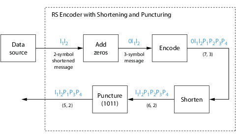
In this figure, the message source outputs two information symbols,
designated by I1I2. (For a BCH
example, the symbols are simply binary bits.) Because the code is a
shortened (7,3) code, a zero must be added ahead of the information symbols,
yielding a three-symbol message of
0I1I2. The modified
message sequence is then RS encoded, and the added information zero is
subsequently removed, which yields a result of
I1I2P1P2P3P4.
(In this example, the parity bits are at the end of the codeword.)
The puncturing operation is governed by the puncture vector, which, in
this case, is 1011. Within the puncture vector, a 1 means that the symbol is
kept, and a 0 means that the symbol is thrown away. In this example, the
puncturing operation removes the second parity symbol, yielding a final
vector of
I1I2P1P3P4.
Decoder Example with Shortening and Puncturing. The following figure shows how the RS encoder operates on a shortened and
punctured codeword.
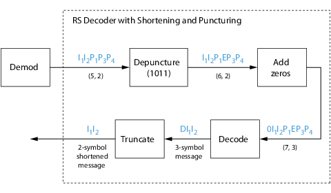
This case corresponds to the encoder operations shown in the figure of the
RS encoder with shortening and puncturing. As shown in the preceding figure,
the encoder receives a (5,2) codeword, because it has been shortened from a
(7,3) codeword by one symbol, and one symbol has also been punctured.
As a first step, the decoder adds an erasure, designated by E, in the
second parity position of the codeword. This corresponds to the puncture
vector 1011. Adding a zero accounts for shortening, in the same way as shown
in the preceding figure. The single erasure does not exceed the
erasure-correcting capability of the code, which can correct four erasures.
The decoding operation results in the three-symbol message
DI1I2. The first symbol is
truncated, as in the preceding figure, yielding a final output of
I1I2.
Encoder Example with Shortening, Puncturing, and Erasures. The following figure shows the decoder operating on the punctured,
shortened codeword, while also correcting erasures generated by the
receiver.
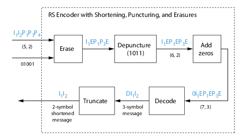
In this figure, demodulator receives the
I1I2P1P3P4
vector that the encoder sent. The demodulator declares that two of the five
received symbols are unreliable enough to be erased, such that symbols 2 and
5 are deemed to be erasures. The 01001 vector, provided by an external
source, indicates these erasures. Within the erasures vector, a 1 means that
the symbol is to be replaced with an erasure symbol, and a 0 means that the
symbol is passed unaltered.
The decoder blocks receive the codeword and the erasure vector, and
perform the erasures indicated by the vector 01001. Within the erasures
vector, a 1 means that the symbol is to be replaced with an erasure symbol,
and a 0 means that the symbol is passed unaltered. The resulting codeword
vector is
I1EP1P3E,
where E is an erasure symbol.
The codeword is then depunctured, according to the puncture vector used in
the encoding operation (i.e., 1011). Thus, an erasure symbol is inserted
between P1 and P3, yielding a
codeword vector of
I1EP1EP3E.
Just prior to decoding, the addition of zeros at the beginning of the
information vector accounts for the shortening. The resulting vector is
0I1EP1EP3E,
such that a (7,3) codeword is sent to the Berlekamp algorithm.
This codeword is decoded, yielding a three-symbol message of
DI1I2 (where D refers to a
dummy symbol). Finally, the removal of the D symbol from the message vector
accounts for the shortening and yields the original
I1I2 vector.
For additional information, see the Reed-Solomon Coding with Erasures, Punctures, and Shortening in Simulink
example.
LDPC Codes
Low-Density Parity-Check (LDPC) codes are linear error control codes with:
-
Sparse parity-check matrices
-
Long block lengths that can attain performance near the Shannon limit
(see LDPC Encoder and LDPC Decoder)
Communications Toolbox performs LDPC Coding using Simulink blocks and MATLAB objects.
The decoding process is done iteratively. If the number of iterations is too
small, the algorithm may not converge. You may need to experiment with the number of
iterations to find an appropriate value for your model. For details on the decoding
algorithm, see Decoding
Algorithm.
Unlike some other codecs, you cannot connect an LDPC decoder directly to the
output of an LDPC encoder, because the decoder requires log-likelihood ratios (LLR).
Thus, you may use a demodulator to compute the LLRs.

Also, unlike other decoders, it is possible (although rare) that the output of the
LDPC decoder does not satisfy all parity checks.
Galois Field Computations
A Galois field is an algebraic field that has a finite number
of members. Galois fields having 2m members are used in
error-control coding and are denoted GF(2m). This section
describes how to work with fields that have 2m members,
where m is an integer between 1 and 16. The subsections in this section are as
follows.
-
Galois Field Terminology
-
Representing Elements of Galois Fields
-
Arithmetic in Galois Fields
-
Logical Operations in Galois Fields
-
Matrix Manipulation in Galois Fields
-
Linear Algebra in Galois Fields
-
Signal Processing Operations in Galois Fields
-
Polynomials over Galois Fields
-
Manipulating Galois Variables
-
Speed and Nondefault Primitive Polynomials
-
Selected Bibliography for Galois Fields
If you need to use Galois fields having an odd number of elements, see Galois Fields of Odd Characteristic.
For more details about specific functions that process arrays of Galois field
elements, see the online reference pages in the documentation for MATLAB or for Communications Toolbox software.
Note
Please note that the Galois field objects do not support the copy method.
MATLAB functions whose generalization to Galois fields is straightforward to
describe do not have reference pages in this manual because the entries would be
identical to those in the MATLAB documentation.
Galois Field Terminology
The discussion of Galois fields in this document uses a few terms that are not
used consistently in the literature. The definitions adopted here appear in van
Lint [4]:
-
A primitive element of
GF(2m) is a cyclic generator of the group
of nonzero elements of GF(2m). This means
that every nonzero element of the field can be expressed as the
primitive element raised to some integer power. -
A primitive polynomial for
GF(2m) is the minimal polynomial of some
primitive element of GF(2m). It is the
binary-coefficient polynomial of smallest nonzero degree having a
certain primitive element as a root in
GF(2m). As a consequence, a primitive
polynomial has degree m and is irreducible.
The definitions imply that a primitive element is a root of a corresponding
primitive polynomial.
Representing Elements of Galois Fields
-
Section Overview
-
Creating a Galois field array
-
Example: Creating Galois Field Variables
-
Example: Representing Elements of GF(8)
-
How Integers Correspond to Galois Field Elements
-
Example: Representing a Primitive Element
-
Primitive Polynomials and Element Representations
Section Overview. This section describes how to create a Galois field
array, which is a MATLAB expression that represents the elements of a Galois field.
This section also describes how MATLAB technical computing software interprets the numbers that you
use in the representation, and includes several examples.
Creating a Galois field array. To begin working with data from a Galois field GF(2^m),
you must set the context by associating the data with crucial information
about the field. The gf function performs this
association and creates a Galois field array in MATLAB. This function accepts as inputs
-
The Galois field data,
x, which is a
MATLAB array whose elements are integers between 0 and
2^m-1. -
(Optional) An integer,
m,
that indicatesxis in the field
GF(2^m). Valid values ofm
are between 1 and 16. The default is 1, which means that the field
is GF(2). -
(Optional) A positive integer that indicates
which primitive polynomial for GF(2^m) you are
using in the representations inx. If you omit
this input argument,gfuses a default
primitive polynomial for GF(2^m). For information
about this argument, see Primitive Polynomials and Element Representations.
The output of the gf function is a variable that
MATLAB recognizes as a Galois field array, rather than an array of
integers. As a result, when you manipulate the variable, MATLAB works within the Galois field you have specified. For example,
if you apply the log function to a Galois field array,
MATLAB computes the logarithm in the Galois field and
not in the field of real or complex numbers.
When MATLAB Implicitly Creates a Galois field
array
Some operations on Galois field arrays require multiple arguments. If you
specify one argument that is a Galois field array and another that is an
ordinary MATLAB array, MATLAB interprets both as Galois field arrays in the same field. It
implicitly invokes the gf function on the ordinary
MATLAB array. This implicit invocation simplifies your syntax because
you can omit some references to the gf function. For an
example of the simplification, see Example: Addition and Subtraction.
Example: Creating Galois Field Variables. The code below creates a row vector whose entries are in the field GF(4),
and then adds the row to itself.
x = 0:3; % A row vector containing integers
m = 2; % Work in the field GF(2^2), or, GF(4).
a = gf(x,m) % Create a Galois array in GF(2^m).

b = a + a % Add a to itself, creating b.
The output is
a = GF(2^2) array. Primitive polynomial = D^2+D+1 (7 decimal)

Array elements =

     0     1     2     3


b = GF(2^2) array. Primitive polynomial = D^2+D+1 (7 decimal)

Array elements =

     0     0     0     0
The output shows the values of the Galois field arrays named
a and b. Each output section
indicates
-
The field containing the variable, namely, GF(2^2) = GF(4).
-
The primitive polynomial for the field. In this case, it is the
toolbox’s default primitive polynomial for GF(4). -
The array of Galois field values that the variable contains. In
particular, the array elements inaare exactly
the elements of the vectorx, and the array
elements inbare four instances of the zero
element in GF(4).
The command that creates b shows how, having defined
the variable a as a Galois field array, you can add
a to itself by using the ordinary
+ operator. MATLAB performs the vectorized addition operation in the field GF(4).
The output shows that
-
Compared to
a,bis in the
same field and uses the same primitive polynomial. It is not
necessary to indicate the field when defining the sum,
b, because MATLAB remembers that information from the definition of the
addends,a. -
The array elements of
bare zeros because the
sum of any value with itself, in a Galois field of
characteristic two, is zero. This result differs from
the sumx + x, which represents an addition
operation in the infinite field of integers.
Example: Representing Elements of GF(8). To illustrate what the array elements in a Galois field array mean, the
table below lists the elements of the field GF(8) as integers and as
polynomials in a primitive element, A. The table should help you interpret a
Galois field array like
gf8 = gf([0:7],3); % Galois vector in GF(2^3)
| Integer Representation | Binary Representation | Element of GF(8) |
|---|---|---|
| 0 | 000 | 0 |
| 1 | 001 | 1 |
| 2 | 010 | A |
| 3 | 011 | A + 1 |
| 4 | 100 | A2 |
| 5 | 101 | A2 + 1 |
| 6 | 110 | A2 + A |
| 7 | 111 | A2 + A + 1 |
How Integers Correspond to Galois Field Elements. Building on the GF(8) example
above, this section explains the interpretation of array elements
in a Galois field array in greater generality. The field
GF(2^m) has 2^m distinct elements,
which this toolbox labels as 0, 1, 2,…, 2^m-1. These
integer labels correspond to elements of the Galois field via a polynomial
expression involving a primitive element of the field. More specifically,
each integer between 0 and 2^m-1 has a binary
representation in m bits. Using the bits in the binary
representation as coefficients in a polynomial, where the least significant
bit is the constant term, leads to a binary polynomial whose order is at
most m-1. Evaluating the binary polynomial at a primitive
element of GF(2^m) leads to an element of the
field.
Conversely, any element of GF(2^m) can be expressed as
a binary polynomial of order at most m-1, evaluated at a
primitive element of the field. The m-tuple of
coefficients of the polynomial corresponds to the binary representation of
an integer between 0 and 2^m.
Below is a symbolic illustration of the correspondence of an integer
X, representable in binary form, with a Galois field
element. Each bk is either zero or
one, while A is a primitive element.
Example: Representing a Primitive Element. The code below defines a variable alph that represents
a primitive element of the field GF(24).
m = 4; % Or choose any positive integer value of m.
alph = gf(2,m) % Primitive element in GF(2^m)
The output is
alph = GF(2^4) array. Primitive polynomial = D^4+D+1 (19 decimal)

Array elements =

     2
The Galois field array alph represents a primitive
element because of the correspondence among
-
The integer 2, specified in the
gf
syntax -
The binary representation of 2, which is 10 (or 0010 using four
bits) -
The polynomial A + 0, where A is a primitive element in this field
(or 0A3 + 0A2
+ A + 0 using the four lowest powers of A)
Primitive Polynomials and Element Representations. This section builds on the discussion in Creating a Galois field array by describing how to specify your own
primitive polynomial when you create a Galois field array. The topics
are
If you perform many computations using a nondefault primitive polynomial,
see Speed and Nondefault Primitive Polynomials.
Specifying the Primitive
Polynomial
The discussion in How Integers Correspond to Galois Field Elements refers to a
primitive element, which is a root of a primitive polynomial of the field.
When you use the gf function to create a Galois field
array, the function interprets the integers in the array with respect to a
specific default primitive polynomial for that field, unless you explicitly
provide a different primitive polynomial. A list of the default primitive
polynomials is on the reference page for the gf function.
To specify your own primitive polynomial when creating a Galois field
array, use a syntax like
c = gf(5,4,25) % 25 indicates the primitive polynomial for GF(16).
instead of
c1= gf(5,4); % Use default primitive polynomial for GF(16).
The extra input argument, 25 in this case, specifies
the primitive polynomial for the field GF(2^m) in a way
similar to the representation described in How Integers Correspond to Galois Field Elements. In this case,
the integer 25 corresponds to a binary representation of 11001, which in
turn corresponds to the polynomial
D4 + D3 + 1.
Note
When you specify the primitive polynomial, the input argument must
have a binary representation using exactly m+1 bits,
not including unnecessary leading zeros. In other words, a primitive
polynomial for GF(2^m) always has order
m.
When you use an input argument to specify the primitive polynomial, the
output reflects your choice by showing the integer value as well as the
polynomial representation.
d = GF(2^4) array. Primitive polynomial = D^4+D^3+1 (25 decimal)

Array elements =

     1     2     3
Note
After you have defined a Galois field array, you cannot change the
primitive polynomial with respect to which MATLAB interprets the array elements.
Finding Primitive
Polynomials
You can use the primpoly function to find primitive
polynomials for GF(2^m) and the
isprimitive function to determine whether a
polynomial is primitive for GF(2^m). The code below
illustrates.
m = 4;
defaultprimpoly = primpoly(m) % Default primitive poly for GF(16)
allprimpolys = primpoly(m,'all') % All primitive polys for GF(16)
i1 = isprimitive(25) % Can 25 be the prim_poly input in gf(...)?
i2 = isprimitive(21) % Can 21 be the prim_poly input in gf(...)?
The output is below.
Primitive polynomial(s) =

D^4+D^1+1

defaultprimpoly =

    19

Primitive polynomial(s) =

D^4+D^1+1
D^4+D^3+1
allprimpolys =

    19
    25

i1 =

     1

i2 =

     0
Effect of Nondefault Primitive Polynomials on
Numerical Results
Most fields offer multiple choices for the primitive polynomial that helps
define the representation of members of the field. When you use the
gf function, changing the primitive polynomial
changes the interpretation of the array elements and, in turn, changes the
results of some subsequent operations on the Galois field array. For
example, exponentiation of a primitive element makes it easy to see how the
primitive polynomial affects the representations of field elements.
a11 = gf(2,3); % Use default primitive polynomial of 11.
a13 = gf(2,3,13); % Use D^3+D^2+1 as the primitive polynomial.
z = a13.^3 + a13.^2 + 1 % 0 because a13 satisfies the equation
nz = a11.^3 + a11.^2 + 1 % Nonzero. a11 does not satisfy equation.
The output below shows that when the primitive polynomial has integer
representation 13, the Galois field array satisfies a
certain equation. By contrast, when the primitive polynomial has integer
representation 11, the Galois field array fails to
satisfy the equation.
z = GF(2^3) array. Primitive polynomial = D^3+D^2+1 (13 decimal)

Array elements =

     0


nz = GF(2^3) array. Primitive polynomial = D^3+D+1 (11 decimal)

Array elements =

     6
The output when you try this example might also include a warning about
lookup tables. This is normal if you did not use the
gftable function to optimize computations involving
a nondefault primitive polynomial of 13.
Arithmetic in Galois Fields
-
Section Overview
-
Example: Addition and Subtraction
-
Example: Multiplication
-
Example: Division
-
Example: Exponentiation
-
Example: Elementwise Logarithm
Section Overview. You can perform arithmetic operations on Galois field arrays by using
familiar MATLAB operators, listed in the table below. Whenever you operate on
a pair of Galois field arrays, both arrays must be in the same Galois field.
| Operation | Operator |
|---|---|
| Addition | +
|
| Subtraction | -
|
| Elementwise multiplication | .*
|
| Matrix multiplication | *
|
| Elementwise left division | ./
|
| Elementwise right division | .
|
| Matrix left division | /
|
| Matrix right division | |
| Elementwise exponentiation | .^
|
| Elementwise logarithm | log()
|
| Exponentiation of a square Galois matrix by a scalar integer |
^
|
For multiplication and division of polynomials over a Galois field, see
Addition and Subtraction of Polynomials.
Example: Addition and Subtraction. The code below adds two Galois field arrays to create an addition table
for GF(8). Addition uses the ordinary + operator. The
code below also shows how to index into the array addtb
to find the result of adding 1 to the elements of GF(8).
m = 3;
e = repmat([0:2^m-1],2^m,1);
f = gf(e,m); % Create a Galois array.
addtb = f + f' % Add f to its own matrix transpose.

addone = addtb(2,:); % Assign 2nd row to the Galois vector addone.
The output is below.
addtb = GF(2^3) array. Primitive polynomial = D^3+D+1 (11 decimal)

Array elements =

     0     1     2     3     4     5     6     7
     1     0     3     2     5     4     7     6
     2     3     0     1     6     7     4     5
     3     2     1     0     7     6     5     4
     4     5     6     7     0     1     2     3
     5     4     7     6     1     0     3     2
     6     7     4     5     2     3     0     1
     7     6     5     4     3     2     1     0
As an example of reading this addition table, the (7,4) entry in the
addtb array shows that gf(6,3)
plus gf(3,3) equals gf(5,3).
Equivalently, the element A2+A plus the element
A+1 equals the element A2+1. The equivalence
arises from the binary representation of 6 as 110, 3 as 011, and 5 as
101.
The subtraction table, which you can obtain by replacing
+ by -, is the same as
addtb. This is because subtraction and addition are
identical operations in a field of characteristic two.
In fact, the zeros along the main diagonal of addtb
illustrate this fact for GF(8).
Simplifying the Syntax
The code below illustrates scalar expansion and the implicit creation of a
Galois field array from an ordinary MATLAB array. The Galois field arrays h and
h1 are identical, but the creation of
h uses a simpler syntax.
g = gf(ones(2,3),4); % Create a Galois array explicitly.
h = g + 5; % Add gf(5,4) to each element of g.
h1 = g + gf(5*ones(2,3),4) % Same as h.
The output is below.
h1 = GF(2^4) array. Primitive polynomial = D^4+D+1 (19 decimal)

Array elements =

     4     4     4
     4     4     4
Notice that 1+5 is reported as 4 in the Galois field. This is true because
the 5 represents the polynomial expression A2+1,
and 1+(A2+1) in GF(16) is
A2. Furthermore, the integer that represents
the polynomial expression A2 is 4.
Example: Multiplication. The example below multiplies individual elements in a Galois field array
using the .* operator. It then performs matrix
multiplication using the * operator. The elementwise
multiplication produces an array whose size matches that of the inputs. By
contrast, the matrix multiplication produces a Galois scalar because it is
the matrix product of a row vector with a column vector.
m = 5;
row1 = gf([1:2:9],m); row2 = gf([2:2:10],m);
col = row2'; % Transpose to create a column array.
ep = row1 .* row2; % Elementwise product.
mp = row1 * col; % Matrix product.
Multiplication Table for GF(8)
As another example, the code below multiplies two Galois vectors using
matrix multiplication. The result is a multiplication table for
GF(8).
m = 3;
els = gf([0:2^m-1]',m);
multb = els * els' % Multiply els by its own matrix transpose.
The output is below.
multb = GF(2^3) array. Primitive polynomial = D^3+D+1 (11 decimal)

Array elements =

     0     0     0     0     0     0     0     0
     0     1     2     3     4     5     6     7
     0     2     4     6     3     1     7     5
     0     3     6     5     7     4     1     2
     0     4     3     7     6     2     5     1
     0     5     1     4     2     7     3     6
     0     6     7     1     5     3     2     4
     0     7     5     2     1     6     4     3
Example: Division. The examples below illustrate the four division operators in a Galois
field by computing multiplicative inverses of individual elements and of an
array. You can also compute inverses using inv or using
exponentiation by -1.
Elementwise Division
This example divides 1 by each of the individual elements in a Galois
field array using the ./ and .
operators. These two operators differ only in their sequence of input
arguments. Each quotient vector lists the multiplicative inverses of the
nonzero elements of the field. In this example, MATLAB expands the scalar 1 to the size of nz
before computing; alternatively, you can use as arguments two arrays of the
same size.
m = 5;
nz = gf([1:2^m-1],m); % Nonzero elements of the field
inv1 = 1 ./ nz; % Divide 1 by each element.
inv2 = nz . 1; % Obtain same result using . operator.
Matrix Division
This example divides the identity array by the square Galois field array
mat using the / and
operators. Each quotient matrix is the
multiplicative inverse of mat. Notice how the transpose
operator (') appears in the equivalent operation using
. For square matrices, the sequence of transpose
operations is unnecessary, but for nonsquare matrices, it is
necessary.
m = 5;
mat = gf([1 2 3; 4 5 6; 7 8 9],m);
minv1 = eye(3) / mat; % Compute matrix inverse.
minv2 = (mat'  eye(3)')'; % Obtain same result using  operator.
Example: Exponentiation. The examples below illustrate how to compute integer powers of a Galois
field array. To perform matrix exponentiation on a Galois field array, you
must use a square Galois field array as the base and an ordinary (not
Galois) integer scalar as the exponent.
Elementwise Exponentiation
This example computes powers of a primitive element, A, of a Galois field.
It then uses these separately computed powers to evaluate the default
primitive polynomial at A. The answer of zero shows that A is a root of the
primitive polynomial. The .^ operator exponentiates each
array element independently.
m = 3;
av = gf(2*ones(1,m+1),m); % Row containing primitive element
expa = av .^ [0:m]; % Raise element to different powers.
evp = expa(4)+expa(2)+expa(1) % Evaluate D^3 + D + 1.
The output is below.
evp = GF(2^3) array. Primitive polynomial = D^3+D+1 (11 decimal)

Array elements =

     0
Matrix Exponentiation
This example computes the inverse of a square matrix by raising the matrix
to the power -1. It also raises the square matrix to the powers 2 and
-2.
m = 5;
mat = gf([1 2 3; 4 5 6; 7 8 9],m);
minvs = mat ^ (-1); % Matrix inverse
matsq = mat^2; % Same as mat * mat
matinvssq = mat^(-2); % Same as minvs * minvs
Example: Elementwise Logarithm. The code below computes the logarithm of the elements of a Galois field
array. The output indicates how to express each nonzero
element of GF(8) as a power of the primitive element. The logarithm of the
zero element of the field is undefined.
gf8_nonzero = gf([1:7],3); % Vector of nonzero elements of GF(8)
expformat = log(gf8_nonzero) % Logarithm of each element
The output is
expformat =

     0     1     3     2     6     4     5
As an example of how to interpret the output, consider the last entry in
each vector in this example. You can infer that the element
gf(7,3) in GF(8) can be expressed as either
-
A5, using the last element of
expformat -
A2+A+1, using the binary representation
of 7 as 111. See Example: Representing Elements of GF(8) for more
details.
Logical Operations in Galois Fields
-
Section Overview
-
Testing for Equality
-
Testing for Nonzero Values
Section Overview. You can apply logical tests to Galois field arrays and obtain a logical
array. Some important types of tests are testing for the equality of two
Galois field arrays and testing for nonzero
values in a Galois field array.
Testing for Equality. To compare corresponding elements of two Galois field arrays that have the
same size, use the operators == and
~=. The result is a logical array, each element of which
indicates the truth or falsity of the corresponding elementwise comparison.
If you use the same operators to compare a scalar with a Galois field array,
MATLAB technical computing software compares the scalar with each
element of the array, producing a logical array of the same size.
m = 5; r1 = gf([1:3],m); r2 = 1 ./ r1;
lg1 = (r1 .* r2 == [1 1 1]) % Does each element equal one?
lg2 = (r1 .* r2 == 1) % Same as above, using scalar expansion
lg3 = (r1 ~= r2) % Does each element differ from its inverse?
The output is below.
lg1 =

     1     1     1


lg2 =

     1     1     1


lg3 =

     0     1     1
Comparison of isequal and ==
To compare entire arrays and obtain a logical scalar
result rather than a logical array, use the built-in
isequal function. However,
isequal uses strict rules for its comparison, and
returns a value of 0 (false) if you compare
-
A Galois field array with an ordinary MATLAB array, even if the values of the underlying array
elements match -
A scalar with a nonscalar array, even if all elements in the array
match the scalar
The example below illustrates this difference between
== and isequal.
m = 5; r1 = gf([1:3],m); r2 = 1 ./ r1;
lg4 = isequal(r1 .* r2, [1 1 1]); % False
lg5 = isequal(r1 .* r2, gf(1,m)); % False
lg6 = isequal(r1 .* r2, gf([1 1 1],m)); % True
Testing for Nonzero Values. To test for nonzero values in a Galois vector, or in the columns of a
Galois field array that has more than one row, use the
any or all function. These two
functions behave just like the ordinary MATLAB functions any and
all, except that they consider only the underlying
array elements while ignoring information about which Galois field the
elements are in. Examples are below.
m = 3; randels = gf(randi([0 2^m-1],6,1),m);
if all(randels) % If all elements are invertible
    invels = randels . 1; % Compute inverses of elements.
else
    disp('At least one element was not invertible.');
end
alph = gf(2,4);
poly = 1 + alph + alph^3;
if any(poly) % If poly contains a nonzero value
    disp('alph is not a root of 1 + D + D^3.');
end
code = [0:4 4 0; 3:7 4 5]
if all(code,2) % Is each row entirely nonzero?
    disp('Both codewords are entirely nonzero.');
else
    disp('At least one codeword contains a zero.');
end
Matrix Manipulation in Galois Fields
-
Basic Manipulations of Galois Field Arrays
-
Basic Information About Galois Field Arrays
Basic Manipulations of Galois Field Arrays. Basic array operations on Galois field arrays are in the table below. The
functionality of these operations is analogous to the MATLAB operations having the same syntax.
| Operation | Syntax |
|---|---|
| Index into array, possibly using colon operator instead of a vector of explicit indices |
a(vector) ora(vector,vector1), wherevector and/orvector1 can be« :» instead of a vector |
| Transpose array | a'
|
| Concatenate matrices | [a,b] or[a;b]
|
| Create array having specified diagonal elements |
diag(vector)or diag(vector,k)
|
| Extract diagonal elements | diag(a) ordiag(a,k)
|
| Extract lower triangular part | tril(a) ortril(a,k)
|
| Extract upper triangular part | triu(a) ortriu(a,k)
|
| Change shape of array | reshape(a,k1,k2)
|
The code below uses some of these syntaxes.
m = 4; a = gf([0:15],m);
a(1:2) = [13 13]; % Replace some elements of the vector a.
b = reshape(a,2,8); % Create 2-by-8 matrix.
c = [b([1 1 2],1:3); a(4:6)]; % Create 4-by-3 matrix.
d = [c, a(1:4)']; % Create 4-by-4 matrix.
dvec = diag(d); % Extract main diagonal of d.
dmat = diag(a(5:9)); % Create 5-by-5 diagonal matrix
dtril = tril(d); % Extract upper and lower triangular
dtriu = triu(d); % parts of d.
Basic Information About Galois Field Arrays. You can determine the length of a Galois vector or the size of any Galois
field array using the length and
size functions. The functionality for Galois field
arrays is analogous to that of the MATLAB operations on ordinary arrays, except that the output
arguments from size and length are
always integers, not Galois field arrays. The code below illustrates the use
of these functions.
m = 4; e = gf([0:5],m); f = reshape(e,2,3);
lne = length(e); % Vector length of e
szf = size(f); % Size of f, returned as a two-element row
[nr,nc] = size(f); % Size of f, returned as two scalars
nc2 = size(f,2); % Another way to compute number of columns
Positions of Nonzero Elements
Another type of information you might want to determine from a Galois
field array are the positions of nonzero elements. For an ordinary
MATLAB array, you might use the find function.
However, for a Galois field array, you should use find
in conjunction with the ~= operator, as
illustrated.
x = [0 1 2 1 0 2]; m = 2; g = gf(x,m);
nzx = find(x); % Find nonzero values in the ordinary array x.
nzg = find(g~=0); % Find nonzero values in the Galois array g.
Linear Algebra in Galois Fields
-
Inverting Matrices and Computing Determinants
-
Computing Ranks
-
Factoring Square Matrices
-
Solving Linear Equations
Inverting Matrices and Computing Determinants. To invert a square Galois field array, use the inv
function. Related is the det function, which computes
the determinant of a Galois field array. Both inv and
det behave like their ordinary MATLAB counterparts, except that they perform computations in the
Galois field instead of in the field of complex numbers.
Note
A Galois field array is singular if and only if its determinant is
exactly zero. It is not necessary to consider roundoff errors, as in the
case of real and complex arrays.
The code below illustrates matrix inversion and determinant
computation.
m = 4;
randommatrix = gf(randi([0 2^m-1],4,4),m);
gfid = gf(eye(4),m);
if det(randommatrix) ~= 0
    invmatrix = inv(randommatrix);
    check1 = invmatrix * randommatrix;
    check2 = randommatrix * invmatrix;
    if (isequal(check1,gfid) & isequal(check2,gfid))
        disp('inv found the correct matrix inverse.');
    end
else
    disp('The matrix is not invertible.');
end
The output from this example is either of these two messages, depending on
whether the randomly generated matrix is nonsingular or singular.
inv found the correct matrix inverse.
The matrix is not invertible.
Computing Ranks. To compute the rank of a Galois field array, use the
rank function. It behaves like the ordinary
MATLAB
rank function when given exactly one input argument.
The example below illustrates how to find the rank of square and nonsquare
Galois field arrays.
m = 3;
asquare = gf([4 7 6; 4 6 5; 0 6 1],m);
r1 = rank(asquare);
anonsquare = gf([4 7 6 3; 4 6 5 1; 0 6 1 1],m);
r2 = rank(anonsquare);
[r1 r2]
The output is
The values of r1 and r2 indicate
that asquare has less than full rank but that
anonsquare has full rank.
Factoring Square Matrices. To express a square Galois field array (or a permutation of it) as the
product of a lower triangular Galois field array and an upper triangular
Galois field array, use the lu function. This function
accepts one input argument and produces exactly two or three output
arguments. It behaves like the ordinary MATLAB
lu function when given the same syntax. The example
below illustrates how to factor using lu.
tofactor = gf([6 5 7 6; 5 6 2 5; 0 1 7 7; 1 0 5 1],3);
[L,U]=lu(tofactor); % lu with two output arguments
c1 = isequal(L*U, tofactor) % True
tofactor2 = gf([1 2 3 4;1 2 3 0;2 5 2 1; 0 5 0 0],3);
[L2,U2,P] = lu(tofactor2); % lu with three output arguments
c2 = isequal(L2*U2, P*tofactor2) % True
Solving Linear Equations. To find a particular solution of a linear equation in a Galois field, use
the or / operator on Galois field
arrays. The table below indicates the equation that each operator addresses,
assuming that A and B are previously
defined Galois field arrays.
| Operator | Linear Equation | Syntax | Equivalent Syntax Using |
|---|---|---|---|
Backslash ( |
A * x = B |
x = A B |
Not applicable |
Slash (/) |
x * A = B |
x = B / A |
x = (A'B')' |
The results of the syntax in the table depend on characteristics of the
Galois field array A:
-
If
Ais square and nonsingular, the output
xis the unique solution to the linear
equation. -
If
Ais square and singular, the syntax in the
table produces an error. -
If
Ais not square, MATLAB attempts to find a particular solution. If
A'*AorA*A'is a singular
array, or ifAis a matrix, where the rows
outnumber the columns, that represents an overdetermined system, the
attempt might fail.
Note
An error message does not necessarily indicate that the linear
equation has no solution. You might be able to find a solution by
rephrasing the problem. For example, gf([1 2; 0 0],3) gf([1; produces an error but the mathematically equivalent
0],3)
gf([1 2],3) gf([1],3) does not. The first
syntax fails because gf([1 2; 0 0],3) is a singular
square matrix.
Example: Solving Linear Equations
The examples below illustrate how to find particular solutions of linear
equations over a Galois field.
m = 4;
A = gf(magic(3),m); % Square nonsingular matrix
Awide=[A, 2*A(:,3)]; % 3-by-4 matrix with redundancy on the right
Atall = Awide'; % 4-by-3 matrix with redundancy at the bottom
B = gf([0:2]',m);
C = [B; 2*B(3)];
D = [B; B(3)+1];
thesolution = A  B; % Solution of A * x = B
thesolution2 = B' / A; % Solution of x * A = B'
ck1 = all(A * thesolution == B) % Check validity of solutions.
ck2 = all(thesolution2 * A == B')
% Awide * x = B has infinitely many solutions. Find one.
onesolution = Awide  B;
ck3 = all(Awide * onesolution == B) % Check validity of solution.
% Atall * x = C has a solution.
asolution = Atall  C;
ck4 = all(Atall * asolution == C) % Check validity of solution.
% Atall * x = D has no solution.
notasolution = Atall  D;
ck5 = all(Atall * notasolution == D) % It is not a valid solution.
The output from this example indicates that the validity checks are all
true (1), except for ck5, which is
false (0).
Signal Processing Operations in Galois Fields
-
Section Overview
-
Filtering
-
Convolution
-
Discrete Fourier Transform
Section Overview. You can perform some signal-processing operations on
Galois field arrays, such as filtering, convolution, and
the discrete Fourier
transform.
This section describes how to perform these operations.
Other information about the corresponding operations for ordinary real
vectors is in the Signal Processing Toolbox™ documentation.
Filtering. To filter a Galois vector, use the filter function.
It behaves like the ordinary MATLAB
filter function when given exactly three input
arguments.
The code and diagram below give the impulse response of a particular
filter over GF(2).
m = 1; % Work in GF(2).
b = gf([1 0 0 1 0 1 0 1],m); % Numerator
a = gf([1 0 1 1],m); % Denominator
x = gf([1,zeros(1,19)],m);
y = filter(b,a,x); % Filter x.
figure; stem(y.x); % Create stem plot.
axis([0 20 -.1 1.1])
Convolution. Communications Toolbox software offers two equivalent ways to convolve a pair of
Galois vectors:
-
Use the
convfunction, as described in Multiplication and Division of Polynomials. This works
because convolving two vectors is equivalent to multiplying the two
polynomials whose coefficients are the entries of the
vectors. -
Use the
convmtxfunction to compute the
convolution matrix of one of the vectors, and then multiply that
matrix by the other vector. This works because convolving two
vectors is equivalent to filtering one of the vectors by the other.
The equivalence permits the representation of a digital filter as a
convolution matrix, which you can then multiply by any Galois vector
of appropriate length.
Tip
If you need to convolve large Galois vectors, multiplying by the
convolution matrix might be faster than using
conv.
Example
Computes the convolution matrix for a vector b in
GF(4). Represent the numerator coefficients for a digital filter, and then
illustrate the two equivalent ways to convolve b with
x over the Galois field.
m = 2; b = gf([1 2 3]',m);
n = 3; x = gf(randi([0 2^m-1],n,1),m);
C = convmtx(b,n); % Compute convolution matrix.
v1 = conv(b,x); % Use conv to convolve b with x
v2 = C*x; % Use C to convolve b with x.
Discrete Fourier Transform. The discrete Fourier transform is an important tool in digital signal
processing. This toolbox offers these tools to help you process discrete
Fourier transforms:
-
fft, which transforms a Galois vector -
ifft, which inverts the discrete Fourier
transform on a Galois vector -
dftmtx, which returns a Galois field array
that you can use to perform or invert the discrete Fourier transform
on a Galois vector
In all cases, the vector being transformed must be a Galois vector of
length 2m-1 in the field
GF(2m). The following example illustrates the
use of these functions. You can check, using the
isequal function, that y equals
y1, z equals
z1, and z equals
x.
m = 4;
x = gf(randi([0 2^m-1],2^m-1,1),m); % A vector to transform
alph = gf(2,m);
dm = dftmtx(alph);
idm = dftmtx(1/alph);
y = dm*x; % Transform x using the result of dftmtx.
y1 = fft(x); % Transform x using fft.
z = idm*y; % Recover x using the result of dftmtx(1/alph).
z1 = ifft(y1); % Recover x using ifft.
Tip
If you have many vectors that you want to transform (in the same
field), it might be faster to use dftmtx once and
matrix multiplication many times, instead of using
fft many times.
Polynomials over Galois Fields
-
Section Overview
-
Addition and Subtraction of Polynomials
-
Multiplication and Division of Polynomials
-
Evaluating Polynomials
-
Roots of Polynomials
-
Roots of Binary Polynomials
-
Minimal Polynomials
Section Overview. You can use Galois vectors to represent polynomials in an indeterminate
quantity x, with coefficients in a Galois field. Form the representation by
listing the coefficients of the polynomial in a vector in order of
descending powers of x. For example, the vector
represents the polynomial Ax3 +
1x2 + 0x + (A+1), where
-
A is a primitive element in the field
GF(24). -
x is the indeterminate quantity in the polynomial.
You can then use such a Galois vector to perform arithmetic with, evaluate, and
find roots of
polynomials. You can also find minimal
polynomials of elements of a Galois field.
Addition and Subtraction of Polynomials. To add and subtract polynomials, use + and
- on equal-length Galois vectors that represent the
polynomials. If one polynomial has lower degree than the other, you must pad
the shorter vector with zeros at the beginning so the two vectors have the
same length. The example below shows how to add a degree-one and a
degree-two polynomial.
lin = gf([4 2],3); % A^2 x + A, which is linear in x
linpadded = gf([0 4 2],3); % The same polynomial, zero-padded
quadr = gf([1 4 2],3); % x^2 + A^2 x + A, which is quadratic in x
% Can't do lin + quadr because they have different vector lengths.
sumpoly = [0, lin] + quadr; % Sum of the two polynomials
sumpoly2 = linpadded + quadr; % The same sum
Multiplication and Division of Polynomials. To multiply and divide polynomials, use conv and
deconv on Galois vectors that represent the
polynomials. Multiplication and division of polynomials is equivalent to
convolution and deconvolution of vectors. The deconv
function returns the quotient of the two polynomials as well as the
remainder polynomial. Examples are below.
m = 4;
apoly = gf([4 5 3],m); % A^2 x^2 + (A^2 + 1) x + (A + 1)
bpoly = gf([1 1],m); % x + 1
xpoly = gf([1 0],m); % x
% Product is A^2 x^3 + x^2 + (A^2 + A) x + (A + 1).
cpoly = conv(apoly,bpoly);
[a2,remd] = deconv(cpoly,bpoly); % a2==apoly. remd is zero.
[otherpol,remd2] = deconv(cpoly,xpoly); % remd is nonzero.
The multiplication and division operators in Arithmetic in Galois Fields
multiply elements or matrices, not polynomials.
Evaluating Polynomials. To evaluate a polynomial at an element of a Galois field, use
polyval. It behaves like the ordinary MATLAB
polyval function when given exactly two input
arguments. The example below evaluates a polynomial at several elements in a
field and checks the results using .^ and
.* in the field.
m = 4;
apoly = gf([4 5 3],m); % A^2 x^2 + (A^2 + 1) x + (A + 1)
x0 = gf([0 1 2],m); % Points at which to evaluate the polynomial
y = polyval(apoly,x0)

a = gf(2,m); % Primitive element of the field, corresponding to A.
y2 = a.^2.*x0.^2 + (a.^2+1).*x0 + (a+1) % Check the result.
The output is below.
y = GF(2^4) array. Primitive polynomial = D^4+D+1 (19 decimal)

Array elements =

     3     2    10


y2 = GF(2^4) array. Primitive polynomial = D^4+D+1 (19 decimal)

Array elements =

     3     2    10
The first element of y evaluates the polynomial at
0 and, therefore, returns the polynomial’s constant
term of 3.
Roots of Polynomials. To find the roots of a polynomial in a Galois field, use the
roots function on a Galois vector that represents
the polynomial. This function finds roots that are in the same field that
the Galois vector is in. The number of times an entry appears in the output
vector from roots is exactly its multiplicity as a root
of the polynomial.
Note
If the Galois vector is in GF(2m), the
polynomial it represents might have additional roots in some extension
field GF((2m)k).
However, roots does not find those additional roots
or indicate their existence.
The examples below find roots of cubic polynomials in GF(8).
p = 3; m = 2;
field = gftuple([-1:p^m-2]',m,p); % List of all elements of GF(9)
% Use default primitive polynomial here.
polynomial = [1 0 1 1]; % 1 + x^2 + x^3
rts =gfroots(polynomial,m,p) % Find roots in exponential format
% Check that each one is actually a root.
for ii = 1:3
   root = rts(ii);
   rootsquared = gfmul(root,root,field);
   rootcubed = gfmul(root,rootsquared,field);
   answer(ii)= gfadd(gfadd(0,rootsquared,field),rootcubed,field);
   % Recall that 1 is really alpha to the zero power.
   % If answer = -Inf, then the variable root represents
   % a root of the polynomial.
end
answer
Roots of Binary Polynomials. In the special case of a polynomial having binary coefficients, it is also
easy to find roots that exist in an extension field. This is because the
elements 0 and 1 have the same
unambiguous representation in all fields of characteristic two. To find
roots of a binary polynomial in an extension field, apply the
roots function to a Galois vector in the extension
field whose array elements are the binary coefficients of the
polynomial.
The example below seeks the roots of a binary polynomial in various
fields.
gf2poly = gf([1 1 1],1); % x^2 + x + 1 in GF(2)
noroots = roots(gf2poly); % No roots in the ground field, GF(2)
gf4poly = gf([1 1 1],2); % x^2 + x + 1 in GF(4)
roots4 = roots(gf4poly); % The roots are A and A+1, in GF(4).
gf16poly = gf([1 1 1],4); % x^2 + x + 1 in GF(16)
roots16 = roots(gf16poly); % Roots in GF(16)
checkanswer4 = polyval(gf4poly,roots4); % Zero vector
checkanswer16 = polyval(gf16poly,roots16); % Zero vector
The roots of the polynomial do not exist in GF(2), so
noroots is an empty array. However, the roots of the
polynomial exist in GF(4) as well as in GF(16), so roots4
and roots16 are nonempty.
Notice that roots4 and roots16 are
not equal to each other. They differ in these ways:
-
roots4is a GF(4) array, while
roots16is a GF(16) array. MATLAB keeps track of the underlying field of a Galois field
array. -
The array elements in
roots4and
roots16differ because they use
representations with respect to different primitive polynomials. For
example,2(which represents a primitive element)
is an element of the vectorroots4because the
default primitive polynomial for GF(4) is the same polynomial that
gf4polyrepresents. On the other hand,
2is not an element of
roots16because the primitive element of
GF(16) is not a root of the polynomial that
gf16polyrepresents.
Minimal Polynomials. The minimal polynomial of an element of GF(2m)
is the smallest degree nonzero binary-coefficient polynomial having that
element as a root in GF(2m). To find the minimal
polynomial of an element or a column vector of elements, use the
minpol function.
The code below finds that the minimal polynomial of
gf(6,4) is
D2 + D + 1 and then checks
that gf(6,4) is indeed among the roots of that polynomial
in the field GF(16).
m = 4;
e = gf(6,4);
em = minpol(e) % Find minimal polynomial of e. em is in GF(2).

emr = roots(gf([0 0 1 1 1],m)) % Roots of D^2+D+1 in GF(2^m)
The output is
em = GF(2) array.

Array elements =

     0     0     1     1     1


emr = GF(2^4) array. Primitive polynomial = D^4+D+1 (19 decimal)

Array elements =

     6
     7
To find out which elements of a Galois field share the same minimal
polynomial, use the cosets function.
Manipulating Galois Variables
-
Section Overview
-
Determining Whether a Variable Is a Galois Field Array
-
Extracting Information from a Galois Field Array
-
Use Field Extension Suffixes Appended to Galois Field Array Variables
Section Overview. This section describes techniques for manipulating Galois variables or for
transferring information between Galois field arrays and ordinary
MATLAB arrays.
Note
These techniques are particularly relevant if you write MATLAB file functions that process Galois field arrays. For an
example of this type of usage, enter edit gf/conv in
the Command Window and examine the first several lines of code in the
editor window.
Determining Whether a Variable Is a Galois Field Array. To find out whether a variable is a Galois field array rather than an
ordinary MATLAB array, use the isa function. An
illustration is below.
mlvar = eye(3);
gfvar = gf(mlvar,3);
no = isa(mlvar,'gf'); % False because mlvar is not a Galois array
yes = isa(gfvar,'gf'); % True because gfvar is a Galois array
Extracting Information from a Galois Field Array. To extract the array elements, field order, or primitive polynomial from a
variable that is a Galois field array, append a suffix to the name of the
variable. The table below lists the exact suffixes, which are independent of
the name of the variable.
| Information | Suffix | Output Value |
|---|---|---|
| Array elements | .x |
MATLAB array of type uint16 thatcontains the data values from the Galois field array. |
| Field order | .m |
Integer of type double that indicatesthat the Galois field array is in GF( 2^m). |
| Primitive polynomial | .prim_poly |
Integer of type uint32 that representsthe primitive polynomial. The representation is similar to the description in How Integers Correspond to Galois Field Elements. |
Note
If the output value is an integer data type and you want to convert it
to double for later manipulation, use the
double function.
Use Field Extension Suffixes Appended to Galois Field Array Variables
Extract information from Galois field arrays by using field extension suffixes.
Array elements (.x)
Convert a Galois field array to doubles.
a = GF(2) array.

Array elements =

   1   0
b = double(a.x) % a.x is in uint16
Field Order (.m)
Check that e solves its own minimal polynomial. Create empr as a Galois field array in a field order extension field (.m) by using a vector of binary coefficients of a polynomial (emp.x).
e = gf(6,4);                % An element of GF(16)
emp = minpol(e);            % Minimal polynomial is in GF(2)
empr = roots(gf(emp.x,e.m)) % Find roots of emp in GF(16)
empr = GF(2^4) array. Primitive polynomial = D^4+D+1 (19 decimal)

Array elements =

   6
   7
Primitive polynomial (.prim_poly)
Check that the primitive element gf(2,m) is really a root of the primitive polynomial for the field by confirming the output vector includes 2. Retrieve the primitive polynomial for the field and convert it to a binary vector representation having the appropriate number of bits.
primpoly_int = double(e.prim_poly);
mval = e.m;
primpoly_vect = gf(int2bit(primpoly_int,mval+1)',mval);
containstwo = roots(primpoly_vect)
containstwo = GF(2^4) array. Primitive polynomial = D^4+D+1 (19 decimal)

Array elements =

   2
   3
   4
   5
Speed and Nondefault Primitive Polynomials
Primitive Polynomials and Element Representations describes how to represent elements of a
Galois field with respect to a primitive polynomial of your choice. This section
describes how you can increase the speed of computations involving a Galois
field array that uses a primitive polynomial other than the default primitive
polynomial. The technique is recommended if you perform many such
computations.
The mechanism for increasing the speed is a data file,
userGftable.mat, that some computational functions use to
avoid performing certain computations repeatedly. To take advantage of this
mechanism for your combination of field order (m) and
primitive polynomial (prim_poly):
-
Navigate in the MATLAB application to a folder to which you have write
permission. You can use either thecdfunction or
the Current Folder feature to navigate. -
Define
mandprim_polyas
workspace variables. For example:m = 3; prim_poly = 13; % Examples of valid values
-
Invoke the
gftablefunction:gftable(m,prim_poly); % If you previously defined m and prim_poly
The function revises or creates userGftable.mat in your
current working folder to include data relating to your combination of field
order and primitive polynomial. After you initially invest the time to invoke
gftable, subsequent computations using those values of
m and prim_poly should be
faster.
Note
If you change your current working directory after invoking
gftable, you must place
userGftable.mat on your MATLAB path to ensure that MATLAB can see it. Do this by using the addpath
command to prefix the directory containing
userGftable.mat to your MATLAB path. If you have multiple copies of
userGftable.mat on your path, use
which('userGftable.mat','-all') to find out where
they are and which one MATLAB is using.
To see how much gftable improves the speed of your
computations, you can surround your computations with the
tic and toc functions. See the
gftable reference page for an
example.
Selected Bibliography for Galois Fields
[1] Blahut, Richard E., Theory and Practice
of Error Control Codes, Reading, MA, Addison-Wesley, 1983,
p. 105.
[2] Lang, Serge, Algebra, Third
Edition, Reading, MA, Addison-Wesley, 1993.
[3] Lin, Shu, and Daniel J. Costello, Jr.,
Error Control Coding: Fundamentals and
Applications, Englewood Cliffs, NJ, Prentice-Hall, 1983.
[4] van Lint, J. H., Introduction to Coding
Theory, New York, Springer-Verlag, 1982.
[5] Wicker, Stephen B., Error Control
Systems for Digital Communication and Storage, Upper Saddle
River, NJ, Prentice Hall, 1995.
Galois Fields of Odd Characteristic
A Galois field is an algebraic field having
pm elements, where p is prime and m is a positive
integer. This section describes how to work with Galois fields in which p is
odd. To work with Galois fields having an even number of
elements, see Galois Field
Computations. The subsections in this section are as follows.
-
Galois Field Terminology
-
Representing Elements of Galois Fields
-
Default Primitive Polynomials
-
Converting and Simplifying Element Formats
-
Arithmetic in Galois Fields
-
Polynomials over Prime Fields
-
Other Galois Field Functions
-
Selected Bibliography for Galois Fields
Galois Field Terminology
Throughout this section, p is an odd prime number and m is a positive integer.
Also, this document uses a few terms that are not used consistently in the
literature. The definitions adopted here appear in van Lint [5].
-
A primitive element of
GF(pm) is a cyclic generator of the group
of nonzero elements of GF(pm). This means
that every nonzero element of the field can be expressed as the
primitive element raised to some integer power. Primitive elements are
called A throughout this section. -
A primitive polynomial for
GF(pm) is the minimal polynomial of some
primitive element of GF(pm). As a
consequence, it has degree m and is irreducible.
Representing Elements of Galois Fields
-
Section Overview
-
Exponential Format
-
Polynomial Format
-
List of All Elements of a Galois Field
-
Nonuniqueness of Representations
Section Overview. This section discusses how to represent Galois field elements using this
toolbox’s exponential
format and polynomial
format. It also describes a way to list all
elements of the Galois field, because some functions use such a
list as an input argument. Finally, it discusses the nonuniqueness of
representations of Galois field elements.
The elements of GF(p) can be represented using the integers from 0 to
p-1.
When m is at least 2, GF(pm) is called an
extension field. Integers alone cannot represent the elements of
GF(pm) in a straightforward way. MATLAB technical computing software uses two main conventions for
representing elements of GF(pm): the exponential
format and the polynomial format.
Note
Both the exponential format and the polynomial format are relative to
your choice of a particular primitive element A of
GF(pm).
Exponential Format. This format uses the property that every nonzero element of
GF(pm) can be expressed as
Ac for some integer c between 0 and
pm-2. Higher exponents are not needed,
because the theory of Galois fields implies that every nonzero element of
GF(pm) satisfies the equation
xq-1 = 1 where
q = pm.
The use of the exponential format is shown in the table below.
| Element of GF(pm) |
MATLAB Representation of the Element |
|---|---|
| 0 | -Inf |
| A0 = 1 | 0
|
| A1 | 1
|
| … | … |
Aq-2 whereq = pm
|
q-2
|
Although -Inf is the standard exponential
representation of the zero element, all negative integers are equivalent to
-Inf when used as input
arguments in exponential format. This equivalence can be useful; for
example, see the concise line of code at the end of the section Default Primitive Polynomials.
Note
The equivalence of all negative integers and -Inf
as exponential formats means that, for example, -1 does
not represent A-1,
the multiplicative inverse of A. Instead, -1 represents the zero element
of the field.
Polynomial Format. The polynomial format uses the property that every element of
GF(pm) can be expressed as a polynomial in A
with exponents between 0 and m-1, and coefficients in GF(p). In the
polynomial format, the element
A(1) + A(2) A + A(3) A2 + … + A(m) Am-1
is represented in MATLAB by the vector
[A(1) A(2) A(3) ... A(m)]
Note
The Galois field functions in this toolbox represent a polynomial as a
vector that lists the coefficients in order of
ascending powers of the variable. This is the
opposite of the order that other MATLAB functions use.
List of All Elements of a Galois Field. Some Galois field functions in this toolbox require an argument that lists
all elements of an extension field GF(pm). This
is again relative to a particular primitive element A of
GF(pm). The proper format for the list of
elements is that of a matrix having pm rows, one
for each element of the field. The matrix has m columns, one for each
coefficient of a power of A in the polynomial format shown in Polynomial Format above. The first row contains only zeros
because it corresponds to the zero element in
GF(pm). If k is between 2 and
pm, then the kth row specifies the polynomial
format of the element Ak-2.
The minimal polynomial of A aids in the computation of this matrix,
because it tells how to express Am in terms of
lower powers of A. For example, the table below lists the elements of
GF(32), where A is a root of the primitive
polynomial 2 + 2x + x2. This
polynomial allows repeated use of the substitution
A2 = -2 — 2A = 1 + A
when performing the computations in the middle column of the table.
Elements of GF(9)
| Exponential Format | Polynomial Format | Row of MATLAB Matrix of Elements |
|---|---|---|
| A-Inf | 0 | 0 0
|
| A0 | 1 | 1 0
|
| A1 | A | 0 1 |
| A2 | 1+A | 1 1 |
| A3 | A + A2 = A + 1 + A = 1 + 2A | 1 2 |
| A4 | A + 2A2 = A + 2 + 2A = 2 | 2 0 |
| A5 | 2A | 0 2 |
| A6 | 2A2 = 2 + 2A | 2 2 |
| A7 | 2A + 2A2 = 2A + 2 + 2A = 2 + A | 2 1 |
Example
An automatic way to generate the matrix whose rows are in the third column
of the table above is to use the code below.
p = 3; m = 2;
% Use the primitive polynomial 2 + 2x + x^2 for GF(9).
prim_poly = [2 2 1];
field = gftuple([-1:p^m-2]',prim_poly,p);
The gftuple function is discussed in more detail in
Converting and Simplifying Element Formats.
Nonuniqueness of Representations. A given field has more than one primitive element. If two primitive
elements have different minimal polynomials, then the corresponding matrices
of elements will have their rows in a different order. If the two primitive
elements share the same minimal polynomial, then the matrix of elements of
the field is the same.
Note
You can use whatever primitive element you want, as long as you
understand how the inputs and outputs of Galois field functions depend
on the choice of some primitive polynomial. It is
usually best to use the same primitive polynomial throughout a given
script or function.
Other ways in which representations of elements are not unique arise from
the equations that Galois field elements satisfy. For example, an
exponential format of 8 in GF(9) is really the same as an exponential format
of 0, because
A8 = 1 = A0
in GF(9). As another example, the substitution mentioned just before the
table Elements of GF(9) shows that the
polynomial format [0 0 1] is really the same as the polynomial format [1
1].
Default Primitive Polynomials
This toolbox provides a default primitive polynomial for
each extension field. You can retrieve this polynomial using the
gfprimdf function. The command
prim_poly = gfprimdf(m,p); % If m and p are already defined
produces the standard row-vector representation of the default minimal
polynomial for GF(pm).
For example, the command below shows that the default primitive polynomial for
GF(9) is 2 + x + x2,
not the polynomial used in List of All Elements of a Galois Field.
To generate a list of elements of GF(pm) using the
default primitive polynomial, use the command
field = gftuple([-1:p^m-2]',m,p);
Converting and Simplifying Element Formats
-
Converting to Simplest Polynomial Format
-
Example: Generating a List of Galois Field Elements
-
Converting to Simplest Exponential Format
Converting to Simplest Polynomial Format. The gftuple function produces the simplest polynomial
representation of an element of GF(pm), given
either an exponential representation or a polynomial representation of that
element. This can be useful for generating the list of elements of
GF(pm) that other functions require.
Using gftuple requires three arguments: one
representing an element of GF(pm), one indicating
the primitive polynomial that MATLAB technical computing software should use when computing the
output, and the prime p. The table below indicates how
gftuple behaves when given the first two arguments
in various formats.
Behavior of gftuple Depending on Format of
First Two Inputs
| How to Specify Element | How to Indicate Primitive Polynomial |
What gftuple Produces |
|---|---|---|
| Exponential format; c = any integer | Integer m > 1 | Polynomial format of Ac, where A is a root of the default primitive polynomial for GF(pm) |
Example: tp = = 6
|
||
| Exponential format; c = any integer | Vector of coefficients of primitive polynomial | Polynomial format of Ac, where A is a root of the given primitive polynomial |
Example:polynomial = gfprimdf(2,3); tp = = 6
|
||
| Polynomial format of any degree | Integer m > 1 | Polynomial format of degree < m, using default primitive polynomial for GF(pm) to simplify |
Example: tp =
|
||
| Polynomial format of any degree | Vector of coefficients of primitive polynomial | Polynomial format of degree < m, using the given primitive polynomial for GF(pm) to simplify |
Example:polynomial = gfprimdf(2,3); tp = gftuple([0
|
The four examples that appear in the table above all produce the same
vector tp = [2, 1], but their different inputs to
gftuple correspond to the lines of the table. Each
example expresses the fact that
A6 = 2+A, where A is a root of the
(default) primitive polynomial
2 + x+ x2 for
GF(32).
Example
This example shows how gfconv and
gftuple combine to multiply two polynomial-format
elements of GF(34). Initially,
gfconv multiplies the two polynomials, treating the
primitive element as if it were a variable. This produces a high-order
polynomial, which gftuple simplifies using the
polynomial equation that the primitive element satisfies. The final result
is the simplest polynomial format of the product.
p = 3; m = 4;
a = [1 2 0 1]; b = [2 2 1 2];
notsimple = gfconv(a,b,p) % a times b, using high powers of alpha
simple = gftuple(notsimple,m,p) %Highest exponent of alpha is m-1
The output is below.
notsimple =

     2     0     2     0     0     1     2


simple =

     2     1     0     1
Example: Generating a List of Galois Field Elements. This example applies the conversion functionality to the task of
generating a matrix that lists all elements of a Galois field. A matrix that
lists all field elements is an input argument in functions such as
gfadd and gfmul. The variables
field1 and field2 below have the
format that such functions expect.
p = 5; % Or any prime number
m = 4; % Or any positive integer
field1 = gftuple([-1:p^m-2]',m,p);

prim_poly = gfprimdf(m,p); % Or any primitive polynomial
% for GF(p^m)
field2 = gftuple([-1:p^m-2]',prim_poly,p);
Converting to Simplest Exponential Format. The same function gftuple also produces the simplest
exponential representation of an element of
GF(pm), given either an exponential
representation or a polynomial representation of that element. To retrieve
this output, use the syntax
[polyformat, expformat] = gftuple(...)
The input format and the output polyformat are as in
the table Behavior of gftuple Depending on Format of First Two Inputs. In
addition, the variable expformat contains the simplest
exponential format of the element represented in
polyformat. It is simplest in
the sense that the exponent is either -Inf or a number
between 0 and pm-2.
Example
To recover the exponential format of the element 2 + A that the
previous section considered, use the commands below. In this case,
polyformat contains redundant information, while
expformat contains the desired result.
[polyformat, expformat] = gftuple([2 1],2,3)
polyformat =

     2     1

expformat =

     6
This output appears at first to contradict the information in the table
Elements of GF(9) , but in fact it does
not. The table uses a different primitive element; two plus that primitive
element has the polynomial and exponential formats shown below.
prim_poly = [2 2 1];
[polyformat2, expformat2] = gftuple([2 1],prim_poly,3)
The output below reflects the information in the bottom line of the
table.
polyformat2 =

     2     1


expformat2 =

     7
Arithmetic in Galois Fields
-
Section Overview
-
Arithmetic in Prime Fields
-
Arithmetic in Extension Fields
Section Overview. You can add, subtract, multiply, and divide elements of Galois fields
using the functions gfadd, gfsub,
gfmul, and gfdiv,
respectively. Each of these functions has a mode for prime fields and
a mode for extension
fields.
Arithmetic in Prime Fields. Arithmetic in GF(p) is the same as arithmetic modulo p. The functions
gfadd, gfmul,
gfsub, and gfdiv accept two
arguments that represent elements of GF(p) as integers between 0 and p-1.
The third argument specifies p.
Example: Addition Table for GF(5)
The code below constructs an addition table for GF(5). If
a and b are between 0 and 4, then
the element gfp_add(a+1,b+1) represents the sum
a+b in GF(5). For example, gfp_add(3,5) = because 2+4 is 1 modulo 5.
1
p = 5;
row = 0:p-1;
table = ones(p,1)*row;
gfp_add = gfadd(table,table',p)
The output for this example follows.
gfp_add =

     0     1     2     3     4
     1     2     3     4     0
     2     3     4     0     1
     3     4     0     1     2
     4     0     1     2     3
Other values of p produce tables for different prime
fields GF(p). Replacing gfadd by
gfmul, gfsub, or
gfdiv produces a table for the corresponding
arithmetic operation in GF(p).
Arithmetic in Extension Fields. The same arithmetic functions can add elements of
GF(pm) when m > 1, but the
format of the arguments is more complicated than in the case above. In
general, arithmetic in extension fields is more complicated than arithmetic
in prime fields; see the works listed in Selected Bibliography for Galois Fields for details about how the arithmetic operations work.
When working in extension fields, the functions
gfadd, gfmul,
gfsub, and gfdiv use the first
two arguments to represent elements of GF(pm) in
exponential format. The third argument, which is required, lists all
elements of GF(pm) as described in List of All Elements of a Galois Field. The result is in
exponential format.
Example: Addition Table for GF(9)
The code below constructs an addition table for
GF(32), using exponential formats relative to
a root of the default primitive polynomial for GF(9). If
a and b are between -1 and 7, then
the element gfpm_add(a+2,b+2) represents the sum of
Aa and Ab in
GF(9). For example, gfpm_add(4,6) = 5 because
A2 + A4 = A5
Using the fourth and sixth rows of the matrix field,
you can verify that
A2 + A4 = (1 + 2A) + (2 + 0A) = 3 + 2A = 0 + 2A = A5
modulo 3.
p = 3; m = 2; % Work in GF(3^2).
field = gftuple([-1:p^m-2]',m,p); % Construct list of elements.
row = -1:p^m-2;
table = ones(p^m,1)*row;
gfpm_add = gfadd(table,table',field)
The output is below.
gfpm_add =

  -Inf     0     1     2     3     4     5     6     7
     0     4     7     3     5  -Inf     2     1     6
     1     7     5     0     4     6  -Inf     3     2
     2     3     0     6     1     5     7  -Inf     4
     3     5     4     1     7     2     6     0  -Inf
     4  -Inf     6     5     2     0     3     7     1
     5     2  -Inf     7     6     3     1     4     0
     6     1     3  -Inf     0     7     4     2     5
     7     6     2     4  -Inf     1     0     5     3
Note
If you used a different primitive polynomial, then the tables would
look different. This makes sense because the ordering of the rows and
columns of the tables was based on that particular choice of primitive
polynomial and not on any natural ordering of the elements of
GF(9).
Other values of p and m produce
tables for different extension fields GF(p^m). Replacing
gfadd by gfmul,
gfsub, or gfdiv produces a
table for the corresponding arithmetic operation in
GF(p^m).
Polynomials over Prime Fields
-
Section Overview
-
Cosmetic Changes of Polynomials
-
Polynomial Arithmetic
-
Characterization of Polynomials
-
Roots of Polynomials
Section Overview. A polynomial over GF(p) is a polynomial whose coefficients are elements of
GF(p). Communications Toolbox software provides functions for
-
Changing polynomials in cosmetic
ways -
Performing polynomial
arithmetic -
Characterizing polynomials as primitive or
irreducible -
Finding roots of
polynomials in a Galois fieldNote
The Galois field functions in this toolbox represent a
polynomial over GF(p) for odd values of p as a vector that lists
the coefficients in order of ascending
powers of the variable. This is the opposite of the order that
other MATLAB functions use.
Cosmetic Changes of Polynomials. To display the traditionally formatted polynomial that corresponds to a
row vector containing coefficients, use gfpretty. To
truncate a polynomial by removing all zero-coefficient terms that have
exponents higher than the degree of the polynomial, use
gftrunc. For example,
polynom = gftrunc([1 20 394 10 0 0 29 3 0 0])
gfpretty(polynom)
The output is below.
polynom =

     1    20   394    10     0     0    29     3


                                   2       3       6      7
                   1 + 20 X + 394 X  + 10 X  + 29 X  + 3 X
Note
If you do not use a fixed-width font, then the spacing in the display
might not look correct.
Polynomial Arithmetic. The functions gfadd and gfsub
add and subtract, respectively, polynomials over GF(p). The
gfconv function multiplies polynomials over GF(p).
The gfdeconv function divides polynomials in GF(p),
producing a quotient polynomial and a remainder polynomial. For example, the
commands below show that
2 + x + x2 times
1 + x over the field GF(3) is
2 + 2x2 + x3.
a = gfconv([2 1 1],[1 1],3)
[quot, remd] = gfdeconv(a,[2 1 1],3)
The output is below.
a =

     2     0     2     1


quot =

     1     1

remd =

     0
The previously discussed functions gfadd and
gfsub add and subtract, respectively, polynomials.
Because it uses a vector of coefficients to represent a polynomial,
MATLAB does not distinguish between adding two polynomials and adding
two row vectors elementwise.
Characterization of Polynomials. Given a polynomial over GF(p), the gfprimck function
determines whether it is irreducible and/or primitive. By definition, if it
is primitive then it is irreducible; however, the reverse is not necessarily
true. The gfprimdf and gfprimfd
functions return primitive polynomials.
Given an element of GF(pm), the
gfminpol function computes its minimal polynomial
over GF(p).
Example
For example, the code below reflects the irreducibility of all minimal
polynomials. However, the minimal polynomial of a nonprimitive element is
not a primitive polynomial.
p = 3; m = 4;
% Use default primitive polynomial here.

prim_poly = gfminpol(1,m,p);
ckprim = gfprimck(prim_poly,p);
% ckprim = 1, since prim_poly represents a primitive polynomial.

notprimpoly = gfminpol(5,m,p);
cknotprim = gfprimck(notprimpoly,p);
% cknotprim = 0 (irreducible but not primitive)
% since alpha^5 is not a primitive element when p = 3.

ckreducible = gfprimck([0 1 1],p);
% ckreducible = -1 since the polynomial is reducible.
Roots of Polynomials. Given a polynomial over GF(p), the gfroots function
finds the roots of the polynomial in a suitable extension field
GF(pm). There are two ways to tell
MATLAB the degree m of the extension field
GF(pm), as shown in the following table.
Formats for Second Argument of
gfroots
| Second Argument | Represents |
|---|---|
| A positive integer | m as in GF(pm). MATLAB uses the default primitive polynomial in its computations. |
| A row vector | A primitive polynomial for GF(pm). Here m is the degree of this primitive polynomial. |
Example: Roots of a Polynomial in
GF(9)
The code below finds roots of the polynomial
1 + x2 + x3
in GF(9) and then checks that they are indeed roots. The exponential format
of elements of GF(9) is used throughout.
p = 3; m = 2;
field = gftuple([-1:p^m-2]',m,p); % List of all elements of GF(9)
% Use default primitive polynomial here.
polynomial = [1 0 1 1]; % 1 + x^2 + x^3
rts =gfroots(polynomial,m,p) % Find roots in exponential format
% Check that each one is actually a root.
for ii = 1:3
   root = rts(ii);
   rootsquared = gfmul(root,root,field);
   rootcubed = gfmul(root,rootsquared,field);
   answer(ii)= gfadd(gfadd(0,rootsquared,field),rootcubed,field);
   % Recall that 1 is really alpha to the zero power.
   % If answer = -Inf, then the variable root represents
   % a root of the polynomial.
end
answer
The output shows that A0 (which equals 1),
A5, and A7 are
roots.
roots =

     0
     5
     7


answer =

  -Inf  -Inf  -Inf
See the reference page for gfroots to see how
gfroots can also provide you with the polynomial
formats of the roots and the list of all elements of the field.
Other Galois Field Functions
See the online reference pages for information about these other Galois field
functions in Communications Toolbox software:
-
gfcosets, which produces
cyclotomic cosets -
gffilter, which filters
data using GF(p) polynomials -
gfprimfd, which finds
primitive polynomials -
gfrank, which computes the
rank of a matrix over GF(p) -
gfrepcov, which converts
one binary polynomial representation to another
Selected Bibliography for Galois Fields
[1] Blahut, Richard E., Theory and
Practice of Error Control Codes, Reading, Mass.,
Addison-Wesley, 1983.
[2] Lang, Serge, Algebra,
Third Edition, Reading, Mass., Addison-Wesley, 1993.
[3] Lin, Shu, and Daniel J. Costello, Jr.,
Error Control Coding: Fundamentals and
Applications, Englewood Cliffs, N.J., Prentice-Hall, 1983.
[4] van Lint, J. H., Introduction to
Coding Theory, New York, Springer-Verlag, 1982.
Vidéo pédagogique
Durée : 00:08:25
—Réalisation : 5 mai 2015
—Mise en ligne : 5 mai 2015
- document 1
document 2
document 3 - niveau 1
niveau 2
niveau 3 - audio 1
audio 2
audio 3
This sequence will be about theerror-correcting capacity of a linear code. We describe the way ofconsidering the space Fq^n as a metric space. This metricis necessary to justify the principle of decodingthat is returning the nearest codeword to the received vector. The metric principle isbased on the following concept: the Hamming distancebetween two vectors is the number of coordinates in which they differ.The Hamming weight of a vector isthe number of non-zero coordinates. Here we give some examples.So, the Hamming distancebetween these two vectors is 2, since they have twocoordinates in which they differ.The Hamming distancebetween these two strings is 1 because they just differ inone letter, and the Hamming weight of these vectorsis 2 since it just has two elements which arenon-zero. The Hamming distance is a metric on the vector space Fq^n. This means that thesefunctions satisfy the usual properties of a distance, thatis non-negativity, symmetry, the Hamming distance isinvariable under permutation, and it verifies the triangle inequality. The proof of theseproperties is left as an exercise. A measure for theerror-correcting capability of a linear code is the minimumdistance, that is the least Hamming distance between twodifferent codewords of a linear code. As we will see later, thehigher the minimum distance, the more errors the code can correct. The reason is that theminimum distance determines the packing radius of a code, thatis the largest integer s such that the balls of radius scentered at the codewords are all disjoint.
Intervenant
Thème
Notice
Crédits
Irene Marquez-Corbella (Intervenant), Nicolas Sendrier (Intervenant), Matthieu Finiasz (Intervenant)
Conditions d’utilisation
Ces ressources de cours sont, sauf mention contraire, diffusées sous Licence Creative Commons. L’utilisateur doit mentionner le nom de l’auteur, il peut exploiter l’œuvre sauf dans un contexte commercial et il ne peut apporter de modifications à l’œuvre originale.
Citer cette ressource :
Irene Marquez-Corbella, Nicolas Sendrier, Matthieu Finiasz. Inria. (2015, 5 mai). 1.5. Error Correcting Capacity. [Vidéo]. Canal-U. https://www.canal-u.tv/92683. (Consultée le 9 février 2023)
Contacter
Documentation
- Dans la même collection
- Avec les mêmes intervenants
- Sur le même thème
Dans la même collection
-
Vidéo pédagogique
00:05:39
1.8. Goppa Codes
In this session, we will
talk about another family of codes that have an efficient
decoding algorithm: the Goppa codes. One limitation of the
generalized Reed-Solomon codes is the fact that the -
Vidéo pédagogique
00:05:34
1.9. McEliece Cryptosystem
This is the last session of
the first week of this MOOC. We have already all the ingredients
to talk about code-based cryptography. Recall that in 1976 Diffie
and Hellman published their famous -
Vidéo pédagogique
00:06:37
1.7. Reed-Solomon Codes
Reed-Solomon codes were introduced
by Reed and Solomon in the 1960s. These codes are still
used in storage device, from compact-disc player to
deep-space application. And they are widely used -
Vidéo pédagogique
00:04:46
1.4. Parity Checking
There are two standard
ways to describe a subspace, explicitly by giving a
basis, or implicitly, by the solution space of the set of
homogeneous linear equations. Therefore, there are two
ways of -
Vidéo pédagogique
00:08:13
1.6. Decoding (A Difficult Problem)
The process of correcting
errors and obtaining back the message is called
decoding. In this sequence, we will focus on this process, the decoding. We would like that the
decoder of the received -
Vidéo pédagogique
00:05:50
1.2. Introduction II — Coding Theory
In this session, we will give a brief introduction to Coding Theory. Claude Shannon’s paper from 1948 entitled «A Mathematical Theory of Communication» gave birth to the disciplines of Information
-
Vidéo pédagogique
00:04:14
1.3. Encoding (Linear Transformation)
In this session, we will
talk about the easy map of the
— one-way trapdoor functions
based on error-correcting codes. We suppose that the set of
all messages that we wish to transmit is the set -
Vidéo pédagogique
00:07:18
1.1. Introduction I — Cryptography
Welcome to this MOOC which is entitled: code-based cryptography. This MOOC is divided in five weeks. The first week, we will talk about error-correcting codes and cryptography, this is an introduction
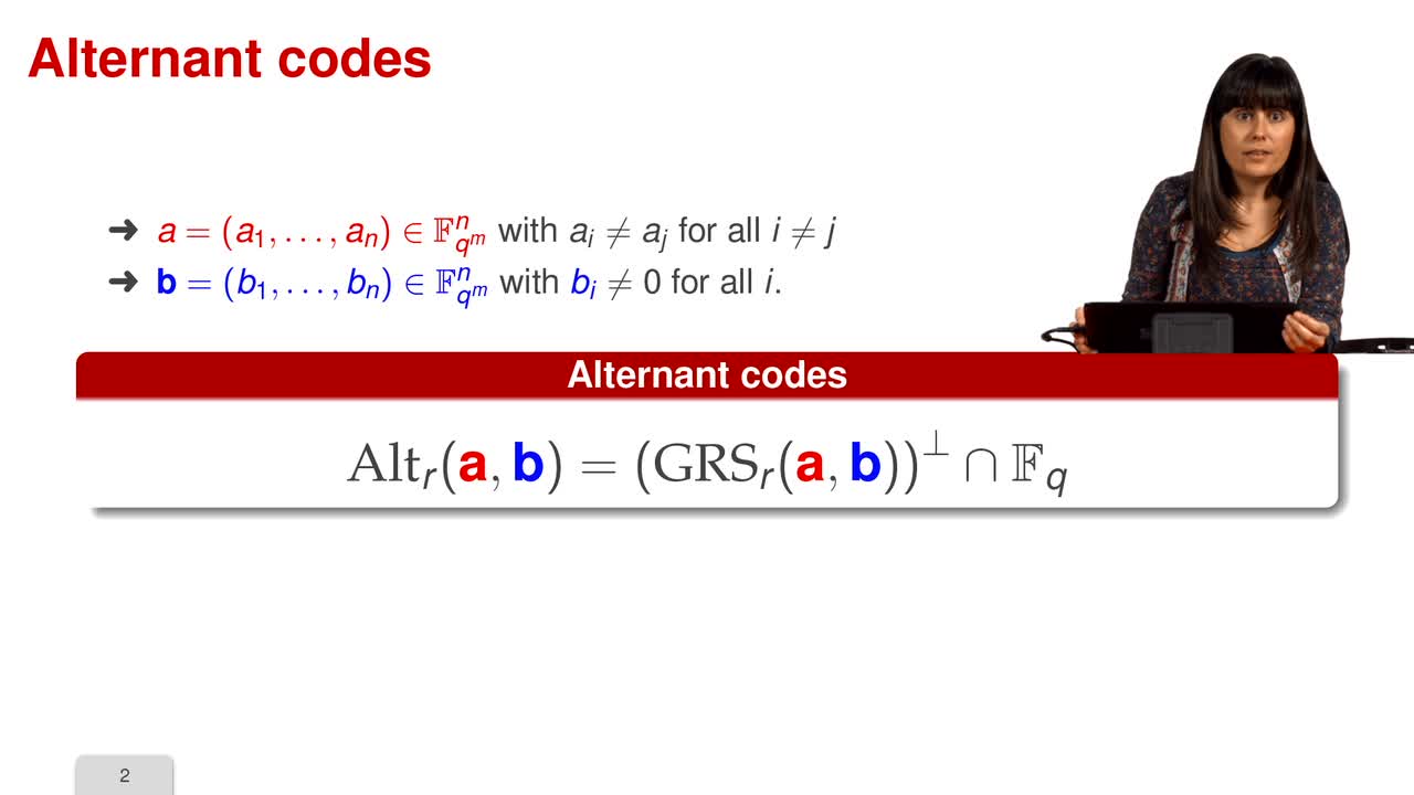
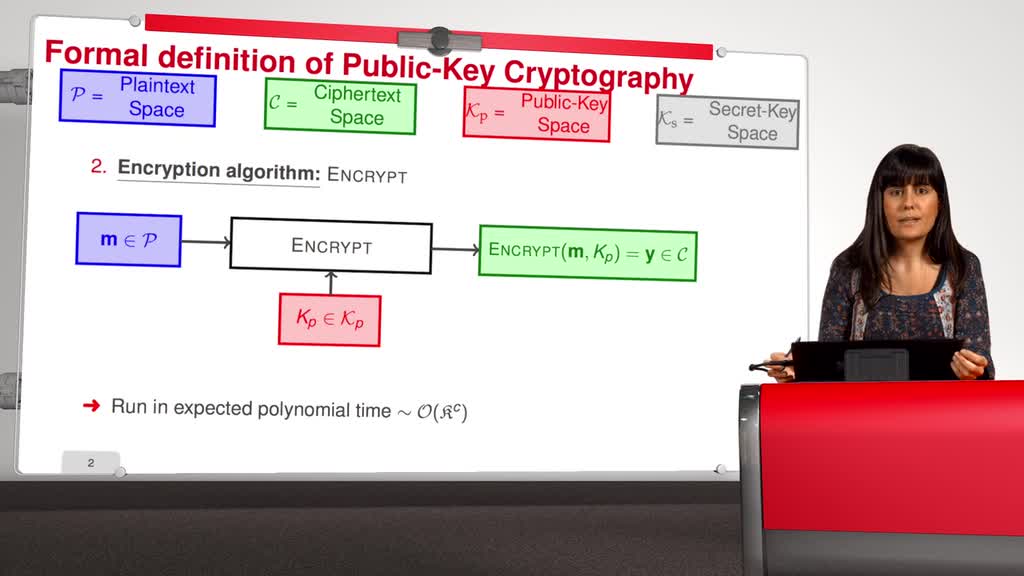
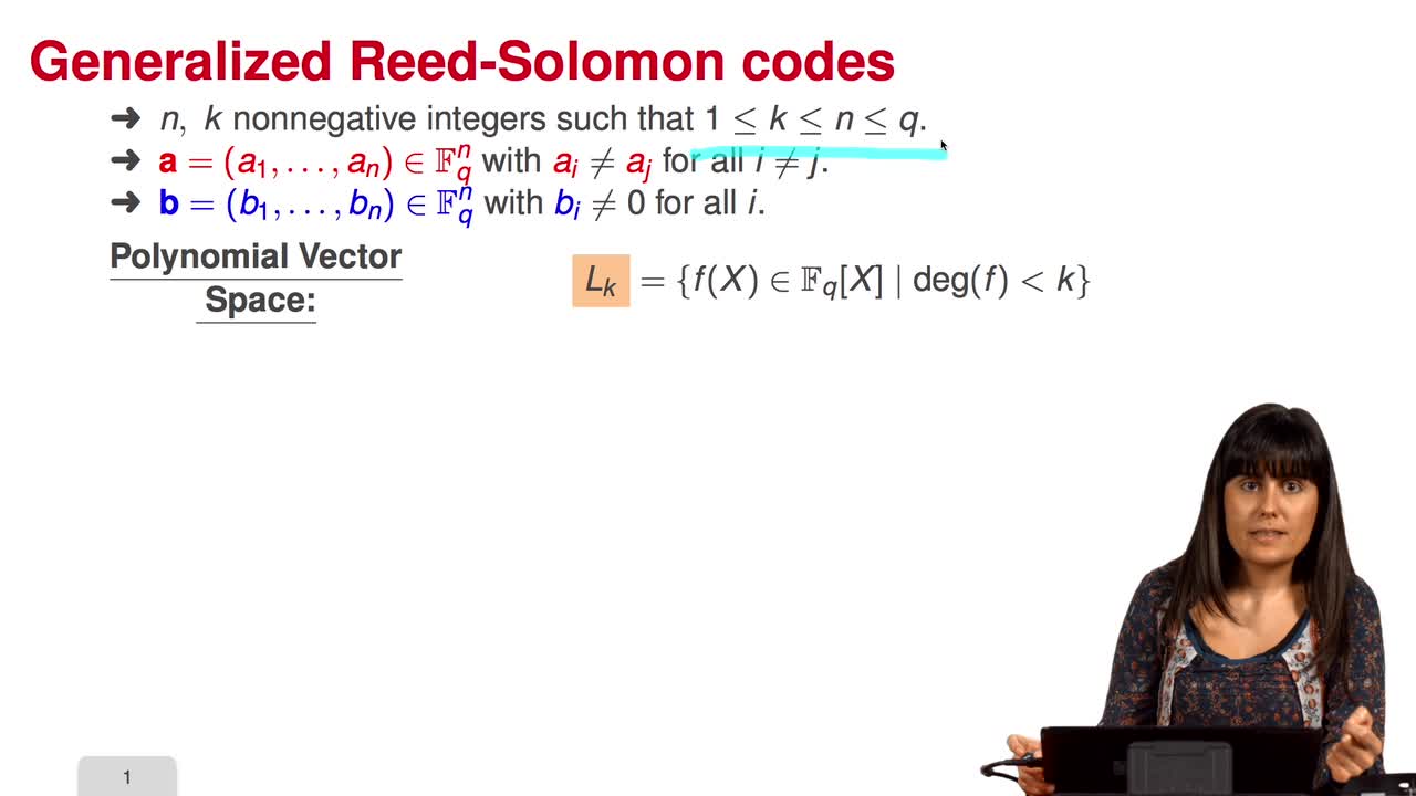
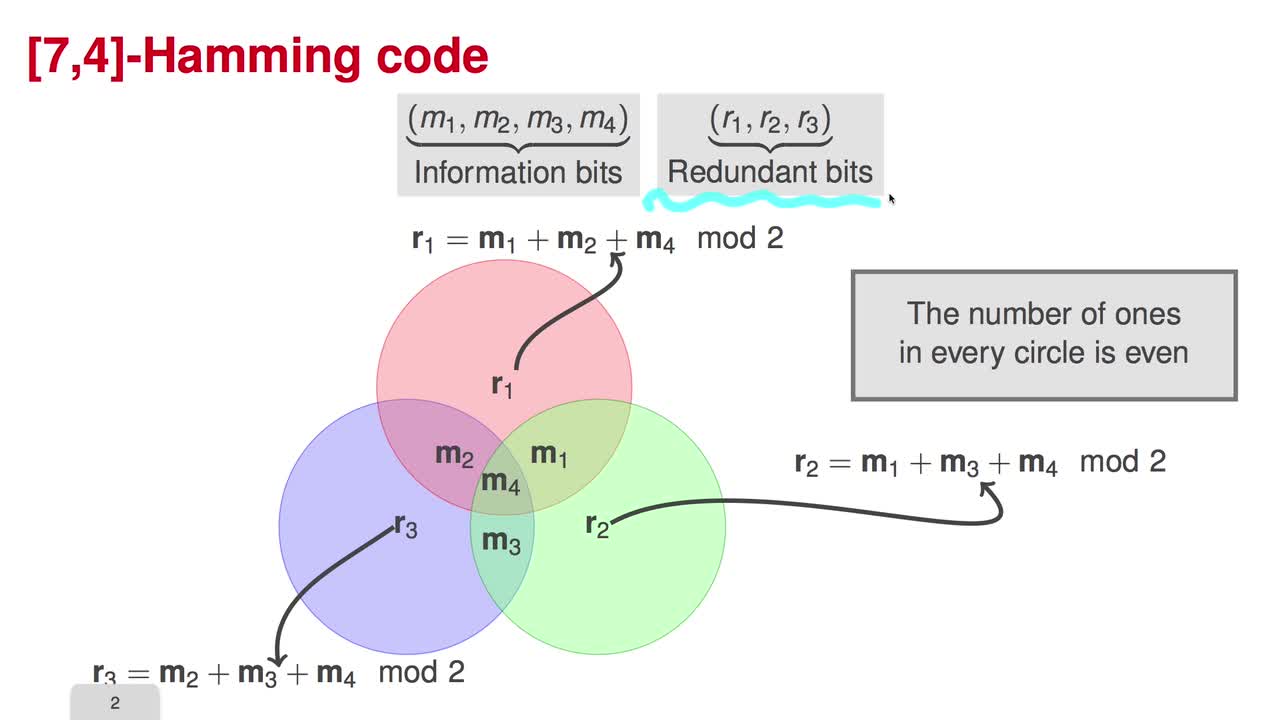
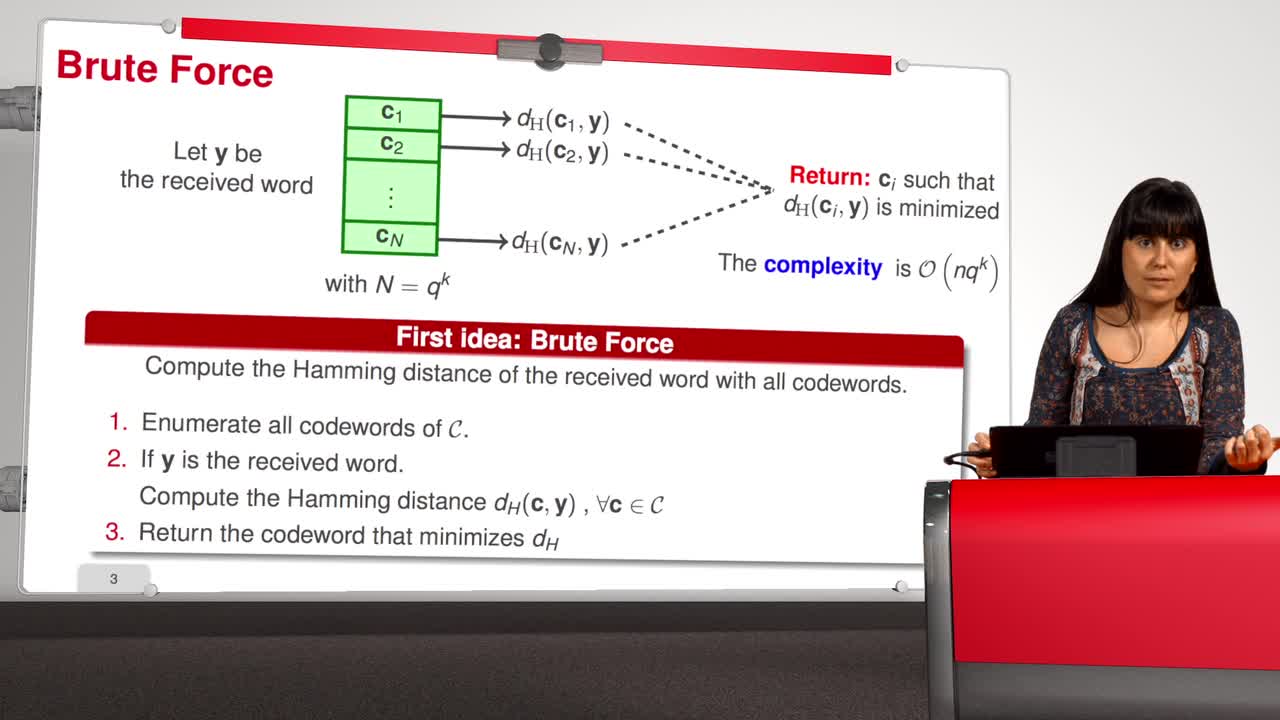
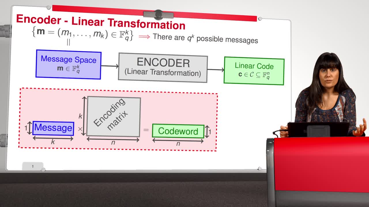
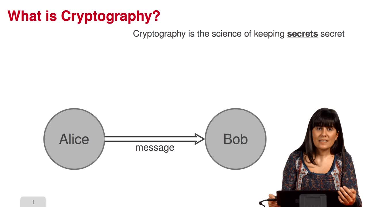
Avec les mêmes intervenants
-
Vidéo pédagogique
00:08:21
5.7. The Fast Syndrome-Based (FSB) Hash Function
In the last session of this
week, we will have a look at the FSB Hash Function which
is built using the one-way function we saw in
the previous session. What are the requirements for
a -
Vidéo pédagogique
00:07:11
5.5. Stern’s Zero-Knowledge Identification Scheme
In this session, we are
going to have a look at Stern’s Zero-Knowledge Identification Scheme. So, what is a
Zero-Knowledge Identification Scheme? An identification scheme
allows a prover to prove -
Vidéo pédagogique
00:05:20
5.6. An Efficient Provably Secure One-Way Function
In this session, we are
going to see how to build an efficient provably secure
one-way function from coding theory. As you know, a one-way
function is a function which is simple to evaluate and -
Vidéo pédagogique
00:04:41
5.4. Parallel-CFS
In this session, I will
present a variant of the CFS signature scheme called
parallel-CFS. We start from a simple question: what
happens if you try to use two different hash functions and
compute -
Vidéo pédagogique
00:04:51
5.3. Attacks against the CFS Scheme
In this session, we will
have a look at the attacks against the CFS signature scheme. As for public-key
encryption, there are two kinds of attacks against signature schemes. First kind of attack is -
Vidéo pédagogique
00:04:32
5.1. Code-Based Digital Signatures
Welcome to the last
week of this MOOC on code-based cryptography. This week, we will be
discussing other cryptographic constructions
relying on coding theory. We have seen how to do
public key -
Vidéo pédagogique
00:04:21
5.2. The Courtois-Finiasz-Sendrier (CFS) Construction
In this session, I am
going to present the Courtois-Finiasz-Sendrier
Construction of a code-based digital signature. In the previous session,
we have seen that it is impossible to hash a
document -
Vidéo pédagogique
00:04:03
4.9. Goppa codes still resist
All the results that we
have seen this week doesn’t mean that code based
cryptography is broken. So in this session we will
see that Goppa code still resists to all these attacks. So recall that -
Vidéo pédagogique
00:06:45
4.8. Attack against Algebraic Geometry codes
In this session, we will present an
attack against Algebraic Geometry codes (AG codes). Algebraic Geometry codes
is determined by a triple. First of all, an
algebraic curve of genus g, then a n -
Vidéo pédagogique
00:05:47
4.7. Attack against Reed-Muller codes
In this session, we will
introduce an attack against binary Reed-Muller codes. Reed-Muller codes were
introduced by Muller in 1954 and, later, Reed provided the
first efficient decoding algorithm -
Vidéo pédagogique
00:05:27
4.6. Attack against GRS codes
In this session we will
discuss the proposal of using generalized Reed-Solomon codes
for the McEliece cryptosystem. As we have already said,
generalized Reed-Solomon codes were proposed in
1986 by -
Vidéo pédagogique
00:05:31
4.5. Error-Correcting Pairs
We present in this session a
general decoding method for linear codes. And we will see it in an example. Let C be a generalized
Reed-Solomon code of dimension k associated to the pair (c, d). Then,
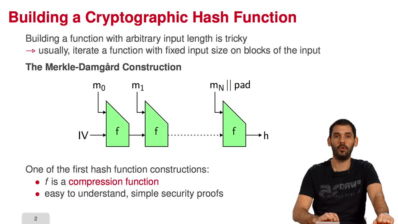

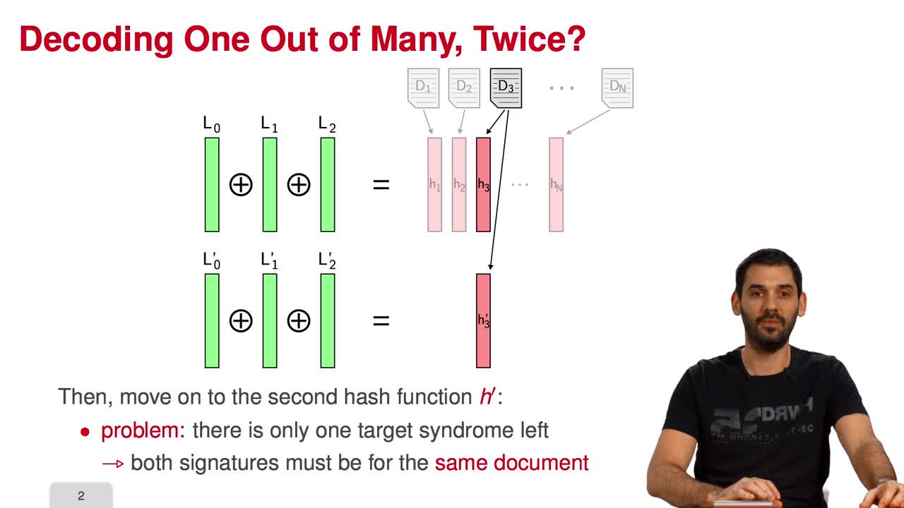

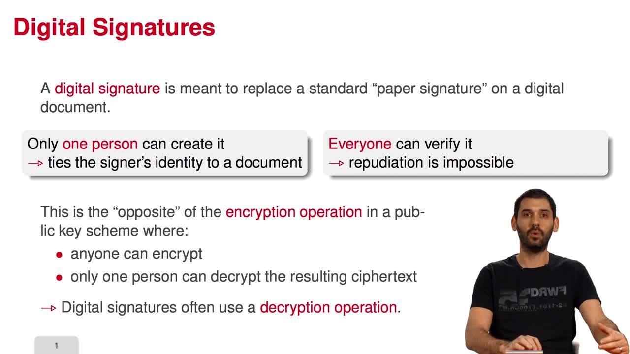
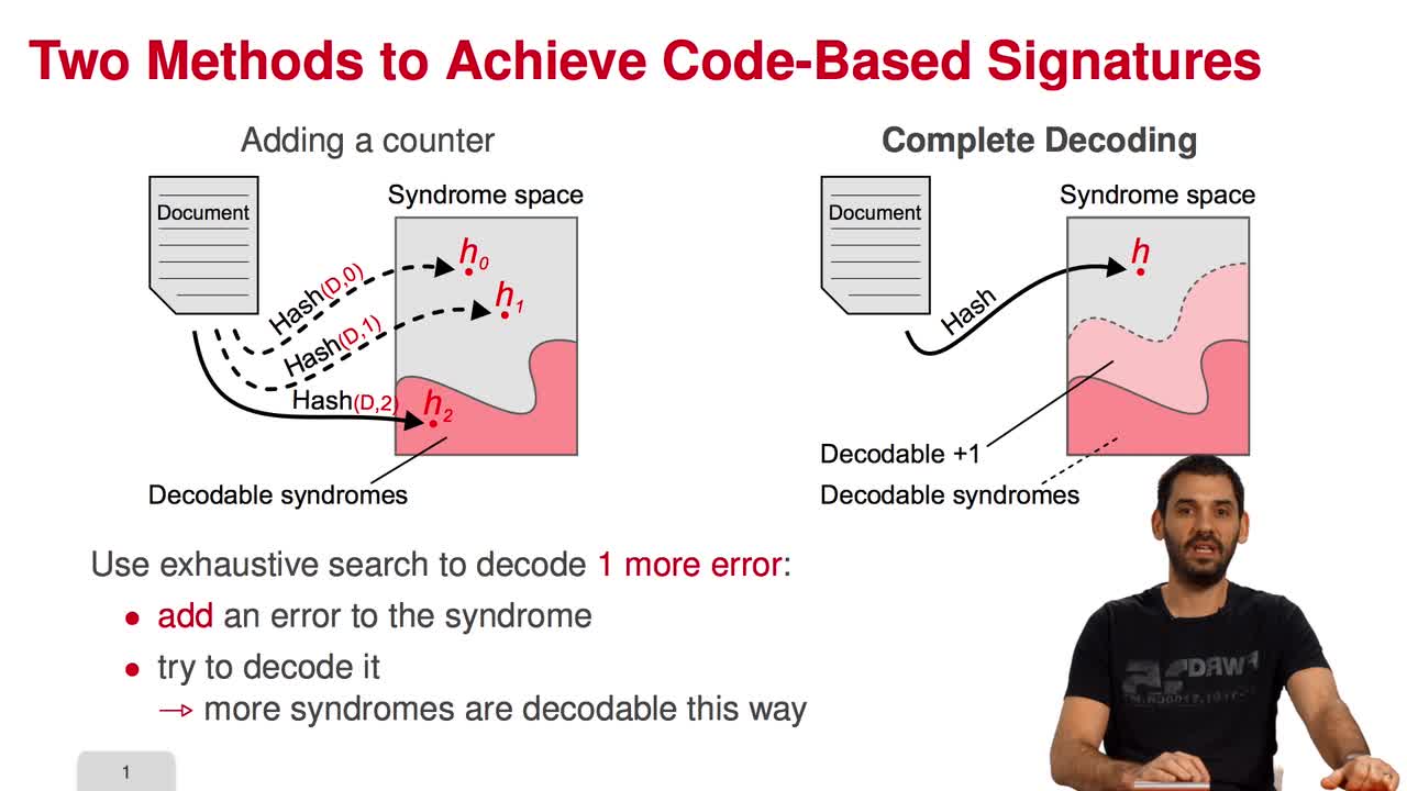
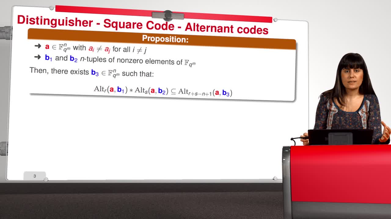

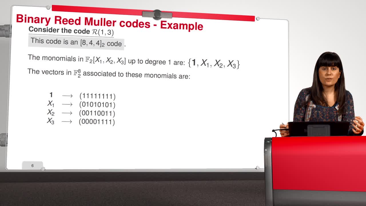
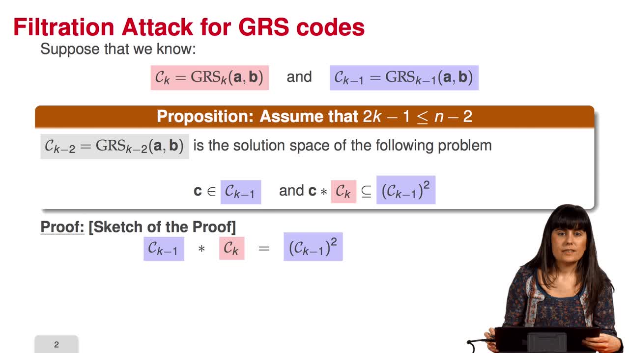
Sur le même thème
-
Retour d’expérience sur l’utilisation croisée de plusieurs archives de fouilles
Dans le cadre d’une thèse de doctorat engagée depuis 2019, une étude historiographique et épistémologique des effets des dispositifs numériques sur l’archéologie et sur les archéologues au cours des
-
Information Structures for Privacy and Fairness
Information Structures for Privacy and Fairness
-
Conférence
01:01:22
AI and Human Decision-Making: An Interdisciplinary Perspective
This seminar will talk about some of the privacy risks of these systems and will describe some recent attacks. It will also discuss why they sometimes fail to deliver. Finally, we will also show that
-
Webinaire sur la rédaction des PGD
Rédaction des Plans de Gestion de Données (PGD) sous l’angle des besoins de la communauté mathématique.
-
Alexandre Booms : « Usage de matériel pédagogique adapté en géométrie : une transposition à interro…
« Usage de matériel pédagogique adapté en géométrie : une transposition à interroger ».
Alexandre Booms, doctorant (Université de Reims Champagne-Ardenne — Cérep UR 4692) -
Conférence
00:09:00
Présentation de la rencontre. A l’heure du numérique « Quelles mesures pour la mesure ? ». Le relev…
Rencontre-Atelier de l’ANR Ornementation Architecturale des Gaules.
À l’heure du numérique, « Quelles mesures pour la mesure ? ». Le relevé des blocs d’architecture décorés et l’apport des outils
-
Conférence
00:47:41
Photogrammétrie : Performances et limitations
Rencontre-Atelier de l’ANR Ornementation Architecturale des Gaules.
À l’heure du numérique, « Quelles mesures pour la mesure ? ». Le relevé des blocs d’architecture décorés et l’apport des outils
-
Conférence
00:35:34
Relever et publier des blocs d’architecture : objectifs et méthodes
Rencontre-Atelier de l’ANR Ornementation Architecturale des Gaules.
À l’heure du numérique, « Quelles mesures pour la mesure ? ». Le relevé des blocs d’architecture décorés et l’apport des outils
-
Conférence
01:01:02
J. Fine — Knots, minimal surfaces and J-holomorphic curves
I
will describe work in progress, parts of which are joint with Marcelo
Alves. Let L be a knot or link in the 3-sphere. I will explain how one
can count minimal surfaces in hyperbolic 4-space -
Conférence
01:07:59
D. Tewodrose — Limits of Riemannian manifolds satisfying a uniform Kato condition
I will present a joint work with G. Carron and I. Mondello where we
study Kato limit spaces. These are metric measure spaces obtained as
Gromov-Hausdorff limits of smooth n-dimensional Riemannian -
Conférence
01:00:08
D. Stern — Harmonic map methods in spectral geometry
Over the last fifty
years, the problem of finding sharp upper bounds for area-normalized
Laplacian eigenvalues on closed surfaces has attracted the attention of
many geometers, due in part to -
Conférence
01:15:11
M. Lesourd — Positive Scalar Curvature on Noncompact Manifolds and the Positive Mass Theorem
The
study of positive scalar curvature on noncompact manifolds has seen
significant progress in the last few years. A major role has been played
by Gromov’s results and conjectures, and in


In information theory and coding theory with applications in computer science and telecommunication, error detection and correction (EDAC) or error control are techniques that enable reliable delivery of digital data over unreliable communication channels. Many communication channels are subject to channel noise, and thus errors may be introduced during transmission from the source to a receiver. Error detection techniques allow detecting such errors, while error correction enables reconstruction of the original data in many cases.

To clean up transmission errors introduced by Earth’s atmosphere (left), Goddard scientists applied Reed–Solomon error correction (right), which is commonly used in CDs and DVDs. Typical errors include missing pixels (white) and false signals (black). The white stripe indicates a brief period when transmission was interrupted.
DefinitionsEdit
Error detection is the detection of errors caused by noise or other impairments during transmission from the transmitter to the receiver.
Error correction is the detection of errors and reconstruction of the original, error-free data.
HistoryEdit
In classical antiquity, copyists of the Hebrew Bible were paid for their work according to the number of stichs (lines of verse). As the prose books of the Bible were hardly ever written in stichs, the copyists, in order to estimate the amount of work, had to count the letters.[1] This also helped ensure accuracy in the transmission of the text with the production of subsequent copies.[2][3] Between the 7th and 10th centuries CE a group of Jewish scribes formalized and expanded this to create the Numerical Masorah to ensure accurate reproduction of the sacred text. It included counts of the number of words in a line, section, book and groups of books, noting the middle stich of a book, word use statistics, and commentary.[1] Standards became such that a deviation in even a single letter in a Torah scroll was considered unacceptable.[4] The effectiveness of their error correction method was verified by the accuracy of copying through the centuries demonstrated by discovery of the Dead Sea Scrolls in 1947–1956, dating from c.150 BCE-75 CE.[5]
The modern development of error correction codes is credited to Richard Hamming in 1947.[6] A description of Hamming’s code appeared in Claude Shannon’s A Mathematical Theory of Communication[7] and was quickly generalized by Marcel J. E. Golay.[8]
IntroductionEdit
All error-detection and correction schemes add some redundancy (i.e., some extra data) to a message, which receivers can use to check consistency of the delivered message, and to recover data that has been determined to be corrupted. Error-detection and correction schemes can be either systematic or non-systematic. In a systematic scheme, the transmitter sends the original data, and attaches a fixed number of check bits (or parity data), which are derived from the data bits by some deterministic algorithm. If only error detection is required, a receiver can simply apply the same algorithm to the received data bits and compare its output with the received check bits; if the values do not match, an error has occurred at some point during the transmission. In a system that uses a non-systematic code, the original message is transformed into an encoded message carrying the same information and that has at least as many bits as the original message.
Good error control performance requires the scheme to be selected based on the characteristics of the communication channel. Common channel models include memoryless models where errors occur randomly and with a certain probability, and dynamic models where errors occur primarily in bursts. Consequently, error-detecting and correcting codes can be generally distinguished between random-error-detecting/correcting and burst-error-detecting/correcting. Some codes can also be suitable for a mixture of random errors and burst errors.
If the channel characteristics cannot be determined, or are highly variable, an error-detection scheme may be combined with a system for retransmissions of erroneous data. This is known as automatic repeat request (ARQ), and is most notably used in the Internet. An alternate approach for error control is hybrid automatic repeat request (HARQ), which is a combination of ARQ and error-correction coding.
Types of error correctionEdit
There are three major types of error correction.[9]
Automatic repeat requestEdit
Automatic repeat request (ARQ) is an error control method for data transmission that makes use of error-detection codes, acknowledgment and/or negative acknowledgment messages, and timeouts to achieve reliable data transmission. An acknowledgment is a message sent by the receiver to indicate that it has correctly received a data frame.
Usually, when the transmitter does not receive the acknowledgment before the timeout occurs (i.e., within a reasonable amount of time after sending the data frame), it retransmits the frame until it is either correctly received or the error persists beyond a predetermined number of retransmissions.
Three types of ARQ protocols are Stop-and-wait ARQ, Go-Back-N ARQ, and Selective Repeat ARQ.
ARQ is appropriate if the communication channel has varying or unknown capacity, such as is the case on the Internet. However, ARQ requires the availability of a back channel, results in possibly increased latency due to retransmissions, and requires the maintenance of buffers and timers for retransmissions, which in the case of network congestion can put a strain on the server and overall network capacity.[10]
For example, ARQ is used on shortwave radio data links in the form of ARQ-E, or combined with multiplexing as ARQ-M.
Forward error correctionEdit
Forward error correction (FEC) is a process of adding redundant data such as an error-correcting code (ECC) to a message so that it can be recovered by a receiver even when a number of errors (up to the capability of the code being used) are introduced, either during the process of transmission or on storage. Since the receiver does not have to ask the sender for retransmission of the data, a backchannel is not required in forward error correction. Error-correcting codes are used in lower-layer communication such as cellular network, high-speed fiber-optic communication and Wi-Fi,[11][12] as well as for reliable storage in media such as flash memory, hard disk and RAM.[13]
Error-correcting codes are usually distinguished between convolutional codes and block codes:
- Convolutional codes are processed on a bit-by-bit basis. They are particularly suitable for implementation in hardware, and the Viterbi decoder allows optimal decoding.
- Block codes are processed on a block-by-block basis. Early examples of block codes are repetition codes, Hamming codes and multidimensional parity-check codes. They were followed by a number of efficient codes, Reed–Solomon codes being the most notable due to their current widespread use. Turbo codes and low-density parity-check codes (LDPC) are relatively new constructions that can provide almost optimal efficiency.
Shannon’s theorem is an important theorem in forward error correction, and describes the maximum information rate at which reliable communication is possible over a channel that has a certain error probability or signal-to-noise ratio (SNR). This strict upper limit is expressed in terms of the channel capacity. More specifically, the theorem says that there exist codes such that with increasing encoding length the probability of error on a discrete memoryless channel can be made arbitrarily small, provided that the code rate is smaller than the channel capacity. The code rate is defined as the fraction k/n of k source symbols and n encoded symbols.
The actual maximum code rate allowed depends on the error-correcting code used, and may be lower. This is because Shannon’s proof was only of existential nature, and did not show how to construct codes which are both optimal and have efficient encoding and decoding algorithms.
Hybrid schemesEdit
Hybrid ARQ is a combination of ARQ and forward error correction. There are two basic approaches:[10]
- Messages are always transmitted with FEC parity data (and error-detection redundancy). A receiver decodes a message using the parity information, and requests retransmission using ARQ only if the parity data was not sufficient for successful decoding (identified through a failed integrity check).
- Messages are transmitted without parity data (only with error-detection information). If a receiver detects an error, it requests FEC information from the transmitter using ARQ, and uses it to reconstruct the original message.
The latter approach is particularly attractive on an erasure channel when using a rateless erasure code.
Error detection schemesEdit
Error detection is most commonly realized using a suitable hash function (or specifically, a checksum, cyclic redundancy check or other algorithm). A hash function adds a fixed-length tag to a message, which enables receivers to verify the delivered message by recomputing the tag and comparing it with the one provided.
There exists a vast variety of different hash function designs. However, some are of particularly widespread use because of either their simplicity or their suitability for detecting certain kinds of errors (e.g., the cyclic redundancy check’s performance in detecting burst errors).
Minimum distance codingEdit
A random-error-correcting code based on minimum distance coding can provide a strict guarantee on the number of detectable errors, but it may not protect against a preimage attack.
Repetition codesEdit
A repetition code is a coding scheme that repeats the bits across a channel to achieve error-free communication. Given a stream of data to be transmitted, the data are divided into blocks of bits. Each block is transmitted some predetermined number of times. For example, to send the bit pattern «1011», the four-bit block can be repeated three times, thus producing «1011 1011 1011». If this twelve-bit pattern was received as «1010 1011 1011» – where the first block is unlike the other two – an error has occurred.
A repetition code is very inefficient, and can be susceptible to problems if the error occurs in exactly the same place for each group (e.g., «1010 1010 1010» in the previous example would be detected as correct). The advantage of repetition codes is that they are extremely simple, and are in fact used in some transmissions of numbers stations.[14][15]
Parity bitEdit
A parity bit is a bit that is added to a group of source bits to ensure that the number of set bits (i.e., bits with value 1) in the outcome is even or odd. It is a very simple scheme that can be used to detect single or any other odd number (i.e., three, five, etc.) of errors in the output. An even number of flipped bits will make the parity bit appear correct even though the data is erroneous.
Parity bits added to each «word» sent are called transverse redundancy checks, while those added at the end of a stream of «words» are called longitudinal redundancy checks. For example, if each of a series of m-bit «words» has a parity bit added, showing whether there were an odd or even number of ones in that word, any word with a single error in it will be detected. It will not be known where in the word the error is, however. If, in addition, after each stream of n words a parity sum is sent, each bit of which shows whether there were an odd or even number of ones at that bit-position sent in the most recent group, the exact position of the error can be determined and the error corrected. This method is only guaranteed to be effective, however, if there are no more than 1 error in every group of n words. With more error correction bits, more errors can be detected and in some cases corrected.
There are also other bit-grouping techniques.
ChecksumEdit
A checksum of a message is a modular arithmetic sum of message code words of a fixed word length (e.g., byte values). The sum may be negated by means of a ones’-complement operation prior to transmission to detect unintentional all-zero messages.
Checksum schemes include parity bits, check digits, and longitudinal redundancy checks. Some checksum schemes, such as the Damm algorithm, the Luhn algorithm, and the Verhoeff algorithm, are specifically designed to detect errors commonly introduced by humans in writing down or remembering identification numbers.
Cyclic redundancy checkEdit
A cyclic redundancy check (CRC) is a non-secure hash function designed to detect accidental changes to digital data in computer networks. It is not suitable for detecting maliciously introduced errors. It is characterized by specification of a generator polynomial, which is used as the divisor in a polynomial long division over a finite field, taking the input data as the dividend. The remainder becomes the result.
A CRC has properties that make it well suited for detecting burst errors. CRCs are particularly easy to implement in hardware and are therefore commonly used in computer networks and storage devices such as hard disk drives.
The parity bit can be seen as a special-case 1-bit CRC.
Cryptographic hash functionEdit
The output of a cryptographic hash function, also known as a message digest, can provide strong assurances about data integrity, whether changes of the data are accidental (e.g., due to transmission errors) or maliciously introduced. Any modification to the data will likely be detected through a mismatching hash value. Furthermore, given some hash value, it is typically infeasible to find some input data (other than the one given) that will yield the same hash value. If an attacker can change not only the message but also the hash value, then a keyed hash or message authentication code (MAC) can be used for additional security. Without knowing the key, it is not possible for the attacker to easily or conveniently calculate the correct keyed hash value for a modified message.
Error correction codeEdit
Any error-correcting code can be used for error detection. A code with minimum Hamming distance, d, can detect up to d − 1 errors in a code word. Using minimum-distance-based error-correcting codes for error detection can be suitable if a strict limit on the minimum number of errors to be detected is desired.
Codes with minimum Hamming distance d = 2 are degenerate cases of error-correcting codes, and can be used to detect single errors. The parity bit is an example of a single-error-detecting code.
ApplicationsEdit
Applications that require low latency (such as telephone conversations) cannot use automatic repeat request (ARQ); they must use forward error correction (FEC). By the time an ARQ system discovers an error and re-transmits it, the re-sent data will arrive too late to be usable.
Applications where the transmitter immediately forgets the information as soon as it is sent (such as most television cameras) cannot use ARQ; they must use FEC because when an error occurs, the original data is no longer available.
Applications that use ARQ must have a return channel; applications having no return channel cannot use ARQ.
Applications that require extremely low error rates (such as digital money transfers) must use ARQ due to the possibility of uncorrectable errors with FEC.
Reliability and inspection engineering also make use of the theory of error-correcting codes.[16]
InternetEdit
In a typical TCP/IP stack, error control is performed at multiple levels:
- Each Ethernet frame uses CRC-32 error detection. Frames with detected errors are discarded by the receiver hardware.
- The IPv4 header contains a checksum protecting the contents of the header. Packets with incorrect checksums are dropped within the network or at the receiver.
- The checksum was omitted from the IPv6 header in order to minimize processing costs in network routing and because current link layer technology is assumed to provide sufficient error detection (see also RFC 3819).
- UDP has an optional checksum covering the payload and addressing information in the UDP and IP headers. Packets with incorrect checksums are discarded by the network stack. The checksum is optional under IPv4, and required under IPv6. When omitted, it is assumed the data-link layer provides the desired level of error protection.
- TCP provides a checksum for protecting the payload and addressing information in the TCP and IP headers. Packets with incorrect checksums are discarded by the network stack, and eventually get retransmitted using ARQ, either explicitly (such as through three-way handshake) or implicitly due to a timeout.
Deep-space telecommunicationsEdit
The development of error-correction codes was tightly coupled with the history of deep-space missions due to the extreme dilution of signal power over interplanetary distances, and the limited power availability aboard space probes. Whereas early missions sent their data uncoded, starting in 1968, digital error correction was implemented in the form of (sub-optimally decoded) convolutional codes and Reed–Muller codes.[17] The Reed–Muller code was well suited to the noise the spacecraft was subject to (approximately matching a bell curve), and was implemented for the Mariner spacecraft and used on missions between 1969 and 1977.
The Voyager 1 and Voyager 2 missions, which started in 1977, were designed to deliver color imaging and scientific information from Jupiter and Saturn.[18] This resulted in increased coding requirements, and thus, the spacecraft were supported by (optimally Viterbi-decoded) convolutional codes that could be concatenated with an outer Golay (24,12,8) code. The Voyager 2 craft additionally supported an implementation of a Reed–Solomon code. The concatenated Reed–Solomon–Viterbi (RSV) code allowed for very powerful error correction, and enabled the spacecraft’s extended journey to Uranus and Neptune. After ECC system upgrades in 1989, both crafts used V2 RSV coding.
The Consultative Committee for Space Data Systems currently recommends usage of error correction codes with performance similar to the Voyager 2 RSV code as a minimum. Concatenated codes are increasingly falling out of favor with space missions, and are replaced by more powerful codes such as Turbo codes or LDPC codes.
The different kinds of deep space and orbital missions that are conducted suggest that trying to find a one-size-fits-all error correction system will be an ongoing problem. For missions close to Earth, the nature of the noise in the communication channel is different from that which a spacecraft on an interplanetary mission experiences. Additionally, as a spacecraft increases its distance from Earth, the problem of correcting for noise becomes more difficult.
Satellite broadcastingEdit
The demand for satellite transponder bandwidth continues to grow, fueled by the desire to deliver television (including new channels and high-definition television) and IP data. Transponder availability and bandwidth constraints have limited this growth. Transponder capacity is determined by the selected modulation scheme and the proportion of capacity consumed by FEC.
Data storageEdit
Error detection and correction codes are often used to improve the reliability of data storage media.[19] A parity track capable of detecting single-bit errors was present on the first magnetic tape data storage in 1951. The optimal rectangular code used in group coded recording tapes not only detects but also corrects single-bit errors. Some file formats, particularly archive formats, include a checksum (most often CRC32) to detect corruption and truncation and can employ redundancy or parity files to recover portions of corrupted data. Reed-Solomon codes are used in compact discs to correct errors caused by scratches.
Modern hard drives use Reed–Solomon codes to detect and correct minor errors in sector reads, and to recover corrupted data from failing sectors and store that data in the spare sectors.[20] RAID systems use a variety of error correction techniques to recover data when a hard drive completely fails. Filesystems such as ZFS or Btrfs, as well as some RAID implementations, support data scrubbing and resilvering, which allows bad blocks to be detected and (hopefully) recovered before they are used.[21] The recovered data may be re-written to exactly the same physical location, to spare blocks elsewhere on the same piece of hardware, or the data may be rewritten onto replacement hardware.
Error-correcting memoryEdit
Dynamic random-access memory (DRAM) may provide stronger protection against soft errors by relying on error-correcting codes. Such error-correcting memory, known as ECC or EDAC-protected memory, is particularly desirable for mission-critical applications, such as scientific computing, financial, medical, etc. as well as extraterrestrial applications due to the increased radiation in space.
Error-correcting memory controllers traditionally use Hamming codes, although some use triple modular redundancy. Interleaving allows distributing the effect of a single cosmic ray potentially upsetting multiple physically neighboring bits across multiple words by associating neighboring bits to different words. As long as a single-event upset (SEU) does not exceed the error threshold (e.g., a single error) in any particular word between accesses, it can be corrected (e.g., by a single-bit error-correcting code), and the illusion of an error-free memory system may be maintained.[22]
In addition to hardware providing features required for ECC memory to operate, operating systems usually contain related reporting facilities that are used to provide notifications when soft errors are transparently recovered. One example is the Linux kernel’s EDAC subsystem (previously known as Bluesmoke), which collects the data from error-checking-enabled components inside a computer system; besides collecting and reporting back the events related to ECC memory, it also supports other checksumming errors, including those detected on the PCI bus.[23][24][25] A few systems[specify] also support memory scrubbing to catch and correct errors early before they become unrecoverable.
See alsoEdit
- Berger code
- Burst error-correcting code
- ECC memory, a type of computer data storage
- Link adaptation
- List of algorithms § Error detection and correction
- List of hash functions
ReferencesEdit
- ^ a b «Masorah». Jewish Encyclopedia.
- ^ Pratico, Gary D.; Pelt, Miles V. Van (2009). Basics of Biblical Hebrew Grammar: Second Edition. Zondervan. ISBN 978-0-310-55882-8.
- ^ Mounce, William D. (2007). Greek for the Rest of Us: Using Greek Tools Without Mastering Biblical Languages. Zondervan. p. 289. ISBN 978-0-310-28289-1.
- ^ Mishneh Torah, Tefillin, Mezuzah, and Sefer Torah, 1:2. Example English translation: Eliyahu Touger. The Rambam’s Mishneh Torah. Moznaim Publishing Corporation.
- ^ Brian M. Fagan (5 December 1996). «Dead Sea Scrolls». The Oxford Companion to Archaeology. Oxford University Press. ISBN 0195076184.
- ^ Thompson, Thomas M. (1983), From Error-Correcting Codes through Sphere Packings to Simple Groups, The Carus Mathematical Monographs (#21), The Mathematical Association of America, p. vii, ISBN 0-88385-023-0
- ^ Shannon, C.E. (1948), «A Mathematical Theory of Communication», Bell System Technical Journal, 27 (3): 379–423, doi:10.1002/j.1538-7305.1948.tb01338.x, hdl:10338.dmlcz/101429, PMID 9230594
- ^ Golay, Marcel J. E. (1949), «Notes on Digital Coding», Proc.I.R.E. (I.E.E.E.), 37: 657
- ^ Gupta, Vikas; Verma, Chanderkant (November 2012). «Error Detection and Correction: An Introduction». International Journal of Advanced Research in Computer Science and Software Engineering. 2 (11). S2CID 17499858.
- ^ a b A. J. McAuley, Reliable Broadband Communication Using a Burst Erasure Correcting Code, ACM SIGCOMM, 1990.
- ^ Shah, Pradeep M.; Vyavahare, Prakash D.; Jain, Anjana (September 2015). «Modern error correcting codes for 4G and beyond: Turbo codes and LDPC codes». 2015 Radio and Antenna Days of the Indian Ocean (RADIO): 1–2. doi:10.1109/RADIO.2015.7323369. ISBN 978-9-9903-7339-4. S2CID 28885076. Retrieved 22 May 2022.
- ^ «IEEE SA — IEEE 802.11ac-2013». IEEE Standards Association.
- ^ «Transition to Advanced Format 4K Sector Hard Drives | Seagate US». Seagate.com. Retrieved 22 May 2022.
- ^ Frank van Gerwen. «Numbers (and other mysterious) stations». Archived from the original on 12 July 2017. Retrieved 12 March 2012.
- ^ Gary Cutlack (25 August 2010). «Mysterious Russian ‘Numbers Station’ Changes Broadcast After 20 Years». Gizmodo. Retrieved 12 March 2012.
- ^ Ben-Gal I.; Herer Y.; Raz T. (2003). «Self-correcting inspection procedure under inspection errors» (PDF). IIE Transactions. IIE Transactions on Quality and Reliability, 34(6), pp. 529-540. Archived from the original (PDF) on 2013-10-13. Retrieved 2014-01-10.
- ^ K. Andrews et al., The Development of Turbo and LDPC Codes for Deep-Space Applications, Proceedings of the IEEE, Vol. 95, No. 11, Nov. 2007.
- ^ Huffman, William Cary; Pless, Vera S. (2003). Fundamentals of Error-Correcting Codes. Cambridge University Press. ISBN 978-0-521-78280-7.
- ^ Kurtas, Erozan M.; Vasic, Bane (2018-10-03). Advanced Error Control Techniques for Data Storage Systems. CRC Press. ISBN 978-1-4200-3649-7.[permanent dead link]
- ^ Scott A. Moulton. «My Hard Drive Died». Archived from the original on 2008-02-02.
- ^ Qiao, Zhi; Fu, Song; Chen, Hsing-Bung; Settlemyer, Bradley (2019). «Building Reliable High-Performance Storage Systems: An Empirical and Analytical Study». 2019 IEEE International Conference on Cluster Computing (CLUSTER): 1–10. doi:10.1109/CLUSTER.2019.8891006. ISBN 978-1-7281-4734-5. S2CID 207951690.
- ^ «Using StrongArm SA-1110 in the On-Board Computer of Nanosatellite». Tsinghua Space Center, Tsinghua University, Beijing. Archived from the original on 2011-10-02. Retrieved 2009-02-16.
- ^ Jeff Layton. «Error Detection and Correction». Linux Magazine. Retrieved 2014-08-12.
- ^ «EDAC Project». bluesmoke.sourceforge.net. Retrieved 2014-08-12.
- ^ «Documentation/edac.txt». Linux kernel documentation. kernel.org. 2014-06-16. Archived from the original on 2009-09-05. Retrieved 2014-08-12.
Further readingEdit
- Shu Lin; Daniel J. Costello, Jr. (1983). Error Control Coding: Fundamentals and Applications. Prentice Hall. ISBN 0-13-283796-X.
- SoftECC: A System for Software Memory Integrity Checking
- A Tunable, Software-based DRAM Error Detection and Correction Library for HPC
- Detection and Correction of Silent Data Corruption for Large-Scale High-Performance Computing
External linksEdit
- The on-line textbook: Information Theory, Inference, and Learning Algorithms, by David J.C. MacKay, contains chapters on elementary error-correcting codes; on the theoretical limits of error-correction; and on the latest state-of-the-art error-correcting codes, including low-density parity-check codes, turbo codes, and fountain codes.
- ECC Page — implementations of popular ECC encoding and decoding routines
Похожие слова: error correcting capability
Синонимы & Антонимы: не найдено
Примеры предложений: error correcting capability |
|
|---|---|
| In order to support Burkina Faso, is prepared to utilize all our military capabilities . |
|
| Her wiring makes her immune to their screening capabilities . |
|
| The advance strengthening of MONUC logistic support capabilities to support the current and foreseen future deployment is of paramount importance. |
|
| Without a more coherent framework, they won’t close the large gap in military spending and capabilities between Europe and the U.S., or make European militaries more effective. |
|
| We have to invest, in fact, in the idea of a meaningful prosperity, providing capabilities for people to flourish. |
|
| Microsoft Band has built — in Global Positioning System (GPS) capabilities , which let you map your activities like running or biking, without having to carry your phone with you. |
|
| For India, which possesses nuclear power, inclusion in the group is important given that its northern enemy, Pakistan, also has nuclear capabilities . |
|
| Militarily, it is a stalemate — which, given the vast imbalance between Russian and Ukrainian capabilities , amounts to a Ukrainian victory. |
|
| Nothing that can detect a ship with the Raza’s capabilities . |
|
| Al Qaeda, for example, has now become a franchised global concern whose capabilities no longer depend on its Afghan base. |
|
| You’ve got some sort of brainwashing capabilities here, don’t you? |
|
| The naval exercises will be closely watched by Russian forces, who are active in the Black Sea, and have vastly improved their surveillance capabilities in Crimea. |
|
| This ship has no offensive capabilities . |
|
| Medvedev is modern and open — minded, but his capabilities fall short of his commitments — this is a widespread view even among the ruling elite. |
|
| Anyway, these are two inventions of mine… Two autonomous mini drones, one with offensive and the other with defensive capabilities . |
|
| To head off the risk of an arms race or military confrontation, both sides must urgently agree to reciprocal measures to limit military capabilities and engage in arms control. |
|
| It is clearly intolerable and unsustainable for all of these countries to depend on the capabilities of Britain, France, and the United States at this time. |
|
| We have nowhere near the capabilities of being able to transport everyone all the way home. |
|
| See our guidelines to using additional capabilities for more info. |
|
| Shishir has been correcting a lot of sentences lately. |
|
| May 7, 2015 Cisco announced plans to buy Tropo, a cloud API platform that simplifies the addition of real — time communications and collaboration capabilities within applications. |
|
| In 2015, the Dutch National Police published their plans to integrate more ‘sensing’ capabilities into routine police work. |
|
| Along with their different capabilities , these two types of digital wallets also come with a difference in security considerations. |
|
| The mineral make — up of this type of soil is responsible for the moisture retaining capabilities . |
|
| Modems used for packet radio vary in throughput and modulation technique, and are normally selected to match the capabilities of the radio equipment in use. |
|
| An oversampled binary image sensor is an image sensor with non — linear response capabilities reminiscent of traditional photographic film. |
|
| In 2000, Deloitte acquired Eclipse to add internet design to its consulting capabilities . |
|
| Lawmakers and others questioned whether the Zumwalt — class costs too much and whether it provides the capabilities that the military needs. |
|
| Take — Two also began taking on distribution capabilities , acquiring various distribution firms such as DirectSoft Australia for the Oceania market. |
|
| The concept of Power in international relations can be described as the degree of resources, capabilities , and influence in international affairs. |
|