with tags
r
vec
cointegration
vars
urca
tsDyn
—
Franz X. Mohr, Created: July 22, 2019, Last update: July 22, 2019
One of the prerequisits for the estimation of a vector autoregressive (VAR) model is that the analysed time series are stationary. However, economic theory suggests that there exist equilibrium relations between economic variables in their levels, which can render these variables stationary without taking differences. This is called cointegration. Since knowing the size of such relationships can improve the results of an analysis, it would be desireable to have an econometric model, which is able to capture them. So-called vector error correction models (VECMs) belong to this class of models. The following text presents the basic concept of VECMs and guides through the estimation of such a model in R.
Model and data
Vector error correction models are very similar to VAR models and can have the following form:
[Delta x_t = Pi x_{t-1} + sum_{l = 1}^{p-1} Gamma_l Delta x_{t-l} + C d_t + epsilon_t,]
where (Delta x) is the first difference of the variables in vector (x), (Pi) is a coefficient matrix of cointegrating relationships, (Gamma) is a coefficient matrix of the lags of differenced variables of (x), (d) is a vector of deterministic terms and (C) its corresponding coefficient matrix. (p) is the lag order of the model in its VAR form and (epsilon) is an error term with zero mean and variance-covariance matrix (Sigma).
The above equation shows that the only difference to a VAR model is the error correction term (Pi x_{t-1}), which captures the effect of how the growth rate of a variable in (x) changes, if one of the variables departs from its equilibrium value. The coefficient matrix (Pi) can be written as the matrix product (Pi = alpha beta^{prime}) so that the error correction term becomes (alpha beta^{prime} x_{t-1}). The cointegration matrix (beta) contains information on the equilibrium relationships between the variables in levels. The vector described by (beta^{prime} x_{t-1}) can be interpreted as the distance of the variables form their equilibrium values. (alpha) is a so-called loading matrix describing the speed at which a dependent variable converges back to its equilibrium value.
Note that (Pi) is assumed to be of reduced rank, which means that (alpha) is a (K times r) matrix and (beta) is a (K^{co} times r) matrix, where (K) is the number of endogenous variables, (K^{co}) is the number of variables in the cointegration term and (r) is the rank of (Pi), which describes the number of cointegrating relationships that exist between the variables. Note that if (r = 0), there is no cointegration between the variables so that (Pi = 0).
To illustrate the estimation of VECMs in R, we use dataset E6 from Lütkepohl (2007), which contains quarterly, seasonally unadjusted time series for German long-term interest and inflation rates from 1972Q2 to 1998Q4. It comes with the bvartools package.
library(bvartools) # Load the package, which contains the data
data("e6") # Load data
plot(e6) # Plot data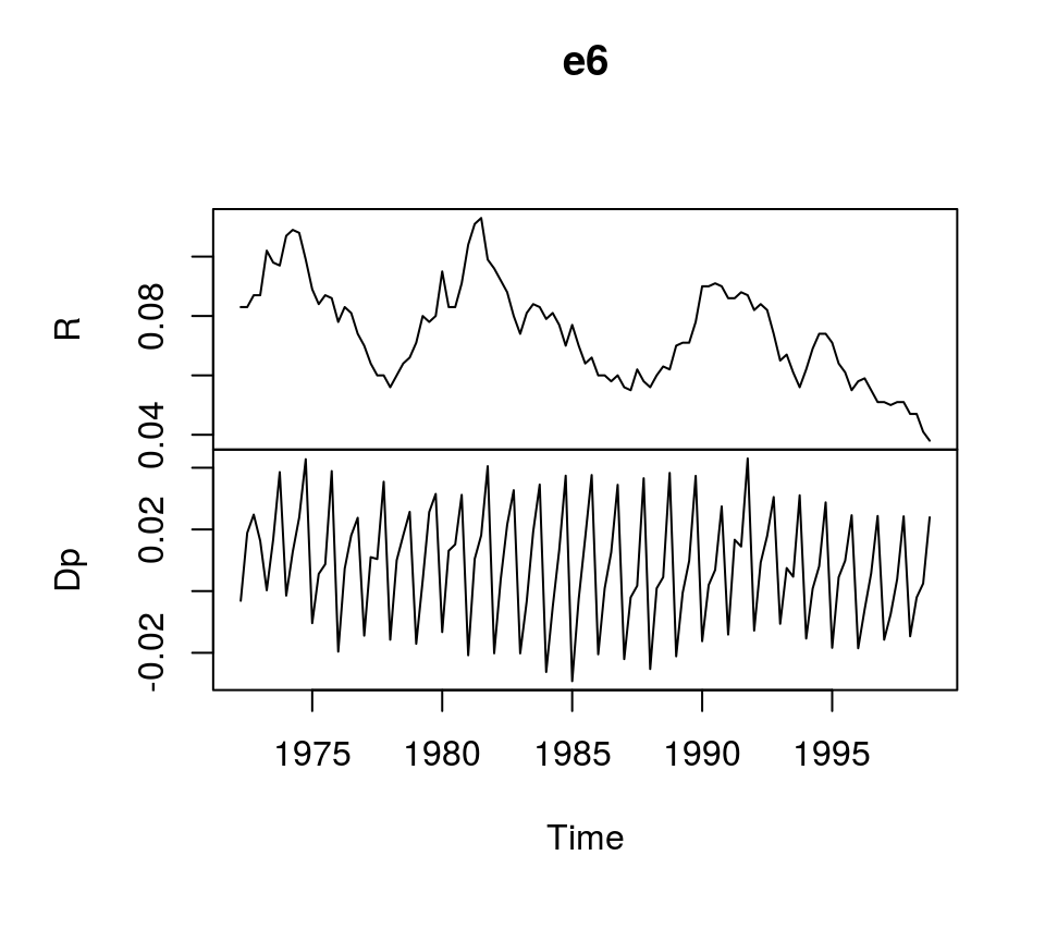
Estimation
There are multiple ways to estimate VEC models. A first approach would be to use ordinary least squares, which yields accurate result, but does not allow to estimate the cointegrating relations among the variables. The estimated generalised least squares (EGLS) approach would be an alternative. However, the most popular estimator for VECMs seems to be the maximum likelihood estimator of Johansen (1995), which is implemented in R by the ca.jo function of the urca package of Pfaff (2008a). Alternatively, function VECM of the tsDyn package of Di Narzo et al. (2020) can be used as well.1
But before the VEC model can be estimated, the lag order (p), the rank of the cointegration matrix (r) and deterministic terms have to be specified. A valid strategy to choose the lag order is to estimated the VAR in levels and choose the lag specification that minimises an Information criterion. Since the time series show strong seasonal pattern, we control for this by specifying season = 4, where 4 is the frequency of the data.
library(vars) # Load package

# Estimate VAR
var_aic <- VAR(e6, type = "const", lag.max = 8, ic = "AIC", season = 4)

# Lag order suggested by AIC
var_aic$p
## AIC(n)
## 4According to the AIC, a lag order of 4 can be used, which is the same value used in Lütkepohl (2007). This means the VEC model corresponding to the VAR in levels has 3 lags. Since the ca.jo function requires the lag order of the VAR model we set K = 4.2
The inclusion of deterministic terms in a VECM is a delicate issue. Without going into detail a common strategy is to add a linear trend to the error correction term and a constant to the non-cointegration part of the equation. For this example we follow Lütkepohl (2007) and add a constant term and seasonal dummies to the non-cointegration part of the equation.
The ca.jo function does not just estimate the VECM. It also calculates the test statistics for different specificaions of (r) and the user can choose between two alternative approaches, the trace and the eigenvalue test. For this example the trace test is used, i.e. type = "trace".
By default, the ca.jo function sets spec = "longrun" This specification would mean that the error correction term does not refer to the first lag of the variables in levels as decribed above, but to the (p-1)th lag instead. By setting spec = "transitory" the first lag will be used instead. Further information on the interpretation the two alternatives can be found in the function’s documentation ?ca.jo.
For further details on VEC modelling I recommend Lütkepohl (2006, Chapters 6, 7 and 8).
library(urca) # Load package

# Estimate
vec <- ca.jo(e6, ecdet = "none", type = "trace",
             K = 4, spec = "transitory", season = 4)

summary(vec)
##
## ######################
## # Johansen-Procedure #
## ######################
##
## Test type: trace statistic , with linear trend
##
## Eigenvalues (lambda):
## [1] 0.15184737 0.03652339
##
## Values of teststatistic and critical values of test:
##
## test 10pct 5pct 1pct
## r <= 1 | 3.83 6.50 8.18 11.65
## r = 0 | 20.80 15.66 17.95 23.52
##
## Eigenvectors, normalised to first column:
## (These are the cointegration relations)
##
## R.l1 Dp.l1
## R.l1 1.000000 1.000000
## Dp.l1 -3.961937 1.700513
##
## Weights W:
## (This is the loading matrix)
##
## R.l1 Dp.l1
## R.d -0.1028717 -0.03938511
## Dp.d 0.1577005 -0.02146119The trace test suggests that (r=1) and the first columns of the estimates of the cointegration relations (beta) and the loading matrix (alpha) correspond to the results of the ML estimator in Lütkepohl (2007, Ch. 7):
# Beta
round(vec@V, 2)
## R.l1 Dp.l1
## R.l1 1.00 1.0
## Dp.l1 -3.96 1.7# Alpha
round(vec@W, 2)## R.l1 Dp.l1
## R.d -0.10 -0.04
## Dp.d 0.16 -0.02However, the estimated coefficients of the non-cointegration part of the model correspond to the results of the EGLS estimator.
round(vec@GAMMA, 2)## constant sd1 sd2 sd3 R.dl1 Dp.dl1 R.dl2 Dp.dl2 R.dl3 Dp.dl3
## R.d 0.01 0.01 0.00 0.00 0.29 -0.16 0.01 -0.19 0.25 -0.09
## Dp.d -0.01 0.02 0.02 0.03 0.08 -0.31 0.01 -0.37 0.04 -0.34The deterministic terms are different from the results in Lütkepohl (2006), because different reference dates are used.
Using the the tsDyn package, estimates of the coefficients can be obtained in the following way:
# Load package
library(tsDyn)

# Obtain constant and seasonal dummies
seas <- gen_vec(data = e6, p = 4, r = 1, const = "unrestricted", seasonal = "unrestricted")
# Lag order p is 4 since gen_vec assumes that p corresponds to VAR form
seas <- seas$data$X[, 7:10]

# Estimate
est_tsdyn <- VECM(e6, lag = 3, r = 1, include = "none", estim = "ML", exogen = seas)

# Print results
summary(est_tsdyn)
## #############
## ###Model VECM
## #############
## Full sample size: 107 End sample size: 103
## Number of variables: 2 Number of estimated slope parameters 22
## AIC -2142.333 BIC -2081.734 SSR 0.005033587
## Cointegrating vector (estimated by ML):
## R Dp
## r1 1 -3.961937
##
##
## ECT R -1 Dp -1
## Equation R -0.1029(0.0471)* 0.2688(0.1062)* -0.2102(0.1581)
## Equation Dp 0.1577(0.0445)*** 0.0654(0.1003) -0.3392(0.1493)*
## R -2 Dp -2 R -3
## Equation R -0.0178(0.1069) -0.2230(0.1276). 0.2228(0.1032)*
## Equation Dp -0.0043(0.1010) -0.3908(0.1205)** 0.0184(0.0975)
## Dp -3 const season.1
## Equation R -0.1076(0.0855) 0.0015(0.0038) 0.0015(0.0051)
## Equation Dp -0.3472(0.0808)*** 0.0102(0.0036)** -0.0341(0.0048)***
## season.2 season.3
## Equation R 0.0089(0.0053). -0.0004(0.0051)
## Equation Dp -0.0179(0.0050)*** -0.0164(0.0048)***Impulse response analyis
The impulse response function of a VECM is usually obtained from its VAR form. The function vec2var of the vars package can be used to transform the output of the ca.jo function into an object that can be handled by the irf function of the vars package. Note that since ur.jo does not set the rank (r) of the cointegration matrix automatically, it has to be specified manually.
# Transform VEC to VAR with r = 1
var <- vec2var(vec, r = 1)
The impulse response function is then calculated in the usual manner by using the irf function.
# Obtain IRF
ir <- irf(var, n.ahead = 20, impulse = "R", response = "Dp",
          ortho = FALSE, runs = 500)

# Plot
plot(ir)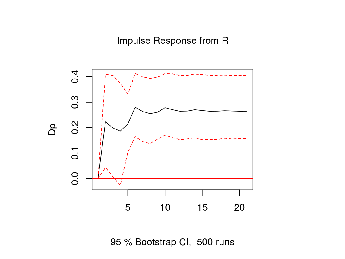
Note that an important difference to stationary VAR models is that the impulse response of a cointegrated VAR model does not neccessarily approach zero, because the variables are not stationary.
References
Lütkepohl, H. (2006). New introduction to multiple time series analysis (2nd ed.). Berlin: Springer.
Di Narzo, A. F., Aznarte, J. L., Stigler, M., &and Tsung-wu, H. (2020). tsDyn: Nonlinear Time Series Models with Regime Switching. R package version 10-1.2. https://CRAN.R-project.org/package=tsDyn
Pfaff, B. (2008a). Analysis of Integrated and Cointegrated Time Series with R. Second Edition. New York: Springer.
Pfaff, B. (2008b). VAR, SVAR and SVEC Models: Implementation Within R Package vars. Journal of Statistical Software 27(4).
[This article was first published on K & L Fintech Modeling, and kindly contributed to R-bloggers]. (You can report issue about the content on this page here)
Want to share your content on R-bloggers? click here if you have a blog, or here if you don’t.
This post explains how to estimate and forecast a Vector Error Correction Model (VECM) model using R. The VECM model consists of VAR model (short-term dynamics) and cointegration (long-term comovement). We use the Johansen cointegration test. The coverage of this post is just a small island of the vast VECM modeling world.
Key Takeaways for Cointegration, VECM, VAR
In general, when variables are non stationary, a VAR model in levels is not appropriate since it is a spurious regression which is a non-interpretable regression. However, although variables are non stationary but when cointegrations exist, a VAR model in levels can be estimated which has a long-term interpretation. In other words, the cointegration indicates one or more long-run equilibriums or stationary relationships among non-stationary variables.
To determine whether VAR model in levels is possible or not, we need to transform VAR model in levels to a VECM model in differences (with error correction terms), to which the Johansen test for cointegration is applied.
In other words, we take the following 4 steps
- construct a VECM model in differences (with error correction terms)
- apply the Johansen test to the VECM model in differences to find out the number of cointegration (r)
- if r = 0, estimate VAR in differences
- if r > 0, estimate VECM model in differences or VAR in levels
in case of 4), the VAR in differences is equal to the VECM model in differences (with no error correction term) since error correction terms does not exist.
In R package, the above steps are implemented in the following way.
- run ca.jo() function with level data for the Johansen cointegration test
- determine the number of cointegrations (r)
- if r = 0, estimate VAR in differences → period.
- if r > 0, apply the cajorls() function to the ca.jo() output to get estimated parameters of the VECM model in differences
- apply vec2var() function to the ca.jo() output to transform the VECM model in differences (with error correction terms) to VAR in levels
- apply predict() function to the transformed VAR model in levels for forecasting
While 4) provides the estimated parameters of VECM model, urca R package provides no function regarding prediction or forecasting. Instead, we use the predict() function in vars R package like 5) and 6). Indeed, for the forecasting purpose, we don’t have to use the cajorls() function since the vec2var() function can take the ca.jo() output as its argument.
Of course, 4), 5), 6) can also be implemented by using the following VECM() function in the tsDyn R package alternatively.
- if r > 0, call VECM() function with level data with the number of cointegrations (r) argument
- apply predict() function to the VECM() output for forecasting
Cointegration
When (x_t) and (y_t) are nonstationary ((I(1))) and if there is a (theta) such that (y_t – theta x_t) is stationary ((I(0))), (x_t) and (y_t) are cointegrated. In other words, although each time series is nonstationary but its linear combination may be stationary. In this case, the cointegration is help the model estimation by augmenting short-run dynamics with long-run equilibriums.
Cointegration test is done by the ca.jo() function in the urca library.
VECM Model
As explained in the previous post, when all variables are non-stationary in level ((X_t)) and there are some cointegrations in level((Pi X_{t})), we use a VECM model which consists of a VAR with stationary growth variables ((Delta X_t)) and error correcting equations with non-stationary level variables ((X_t)).
VECM describes a short-run dynamics by vector autoregression (VAR) as well as a long-run equilibrium by error correcting equations.
[begin{align} Delta X_t = Pi X_{t-1} + sum_{i=1}^{p-1}Gamma_i Delta X_{t-i} + CD_t + epsilon_t end{align}]
where (Delta x) is the first difference of (x), (Pi) is a coefficient matrix of cointegrating relationships. (Gamma_i) is a coefficient matrix of (Delta x_{t-i}), C is a coefficient matrix of a vector of deterministic terms (d_t). (epsilon_t) is an error term with mean zero and variance-covariance matrix (Sigma).
(Pi X_{t-1}) is the first lag of linear combinations of non-stationary level variables or error correction terms (ECT) which represent long-term relationships among non-stationary level variables.
For example, a tri-variate VECM(2) model is represented in the following way.
[begin{align} begin{bmatrix} Delta x_t \ Delta y_t \ Delta z_t end{bmatrix} &= begin{bmatrix} pi_{11} & pi_{12} & pi_{13} \ pi_{21} & pi_{22} & pi_{23} \ pi_{31} & pi_{32} & pi_{33} end{bmatrix} begin{bmatrix} x_{t-1} \ y_{t-1} \ z_{t-1} end{bmatrix} \ &+begin{bmatrix} gamma_{11}^1 & gamma_{12}^1 & gamma_{13}^1 \ gamma_{21}^1 & gamma_{22}^1 & gamma_{23}^1 \ gamma_{31}^1 & gamma_{32}^1 & gamma_{33}^1 end{bmatrix} begin{bmatrix} Delta x_{t-1} \ Delta y_{t-1} \ Delta z_{t-1} end{bmatrix} \ &+begin{bmatrix} gamma_{11}^2 & gamma_{12}^2 & gamma_{13}^2 \ gamma_{21}^2 & gamma_{22}^2 & gamma_{23}^2 \ gamma_{31}^2 & gamma_{32}^2 & gamma_{33}^2 end{bmatrix} begin{bmatrix} Delta x_{t-2} \ Delta y_{t-2} \ Delta z_{t-2} end{bmatrix} \ &+begin{bmatrix} c_{11} & c_{12} \ c_{21} & c_{22} \ c_{31} & c_{32} end{bmatrix} begin{bmatrix} 1 \ d_{t} end{bmatrix} +begin{bmatrix} epsilon_{xt} \ epsilon_{yt} \ epsilon_{zt} end{bmatrix} end{align}]
(Pi X_{t-1}) is the first lag of linear combinations of non-stationary level variables or error correction terms (ECT) which represent long-term relationships among non-stationary level variables.
In particular, the above cointegrating vector ((Pi)) is not unique and is interpreted as a kind of combined coefficient, it is decomposed into 1) a cointegration or equilibrium matrix ((beta)) and 2) a loading or speed matrix ((alpha)) as follows. [begin{align} Pi = alpha beta^{‘} end{align}] Its identification depends on the number of cointegration in the following way.
0) r = 0 (no cointegration)
In the case of no cointegration, since all variables are non-stationary in level, the above VECM model reduces to a VAR model with growth variables.
1) r = 1 (one cointegrating vector)
[begin{align} Pi X_{t} &= begin{bmatrix} pi_{11} & pi_{12} & pi_{13} \ pi_{21} & pi_{22} & pi_{23} \ pi_{31} & pi_{32} & pi_{33} end{bmatrix} begin{bmatrix} x_{t} \ y_{t} \ z_{t} end{bmatrix} \ &= begin{bmatrix} alpha_{11} \ alpha_{21} \ alpha_{31} end{bmatrix} begin{bmatrix} 1 & – beta_{11} & – beta_{12} end{bmatrix} begin{bmatrix} x_t \ y_t \ z_t end{bmatrix} \ &= begin{bmatrix} alpha_{11} \ alpha_{21} \ alpha_{31} end{bmatrix} begin{bmatrix} 1 \ – beta_{11} \ – beta_{12} end{bmatrix}^{‘} begin{bmatrix} x_t \ y_t \ z_t end{bmatrix} = alpha beta^{‘} X_t \ &= begin{bmatrix} alpha_{11} \ alpha_{21} \ alpha_{31} end{bmatrix} begin{bmatrix} x_{t} – beta_{11} y_{t} – beta_{12} z_{t} end{bmatrix} = alpha EC_t end{align}]
2) r = 2 (two cointegrating vectors)
[begin{align} Pi X_{t} &= begin{bmatrix} pi_{11} & pi_{12} & pi_{13} \ pi_{21} & pi_{22} & pi_{23} \ pi_{31} & pi_{32} & pi_{33} end{bmatrix} begin{bmatrix} x_{t} \ y_{t} \ z_{t} end{bmatrix} \ &= begin{bmatrix} alpha_{11} & alpha_{12} \ alpha_{21} & alpha_{22} \ alpha_{31} & alpha_{32} end{bmatrix} begin{bmatrix} 1 & – beta_{11} & – beta_{12} \ 1 & – beta_{21} & – beta_{22} end{bmatrix} begin{bmatrix} x_t \ y_t \ z_t end{bmatrix} \ &= begin{bmatrix} alpha_{11} & alpha_{12} \ alpha_{21} & alpha_{22} \ alpha_{31} & alpha_{32} end{bmatrix} begin{bmatrix} 1 & 1 \ – beta_{11} & – beta_{21} \ – beta_{12} & – beta_{22} end{bmatrix}^{‘} X_t = alpha beta^{‘} X_t \ &= begin{bmatrix} alpha_{11} & alpha_{12} \ alpha_{21} & alpha_{22} \ alpha_{31} & alpha_{32} end{bmatrix} begin{bmatrix} x_{t} – beta_{11} y_{t} – beta_{12} z_{t} \ x_{t} – beta_{21} y_{t} – beta_{22} z_{t} end{bmatrix} = alpha EC_t end{align}]
3) r = 3 (full cointegration)
In the case of full cointegration, since all variables are stationary, the above VECM model reduces to a VAR model with level variables.
Johansen Test for Cointegration
The rank of (Pi) equals the number of its non-zero eigenvalues and the Johansen test provides inference on this number. There are two tests for the number of co-integration relationships.
The first test is the trace test whose test statistic is
- H0 : cointegrating vectors ≤ r
- H1 : cointegrating vectors ≥ r + 1
The second test is the maximum eigenvalue test whose test statistic is given by
- H0 : There are r cointegrating vectors
- H1 : There are r + 1 cointegrating vectors
In both cases, r denotes the number of cointegrations
For this Johansen cointegration test, we can use the ca.jo() function in the urca R package. The following R code shows how to use ca.jo() function with the typical input argument.
|
vecm.model <– ca.jo( data_level, ecdet = “const”, type = “eigen”, K = 2, spec = “transitory”, season = 4, dumvar = NULL) summary(vecm.model) |
Relevant R functions
After running ca.jo() function for the cointegration test, there are three R functions for the estimation of VECM model.
These 3 R functions have the following functionalities.
- vec2var() from package vars : Transform a VECM to VAR in levels
- cajorls() from package urca : OLS regressions of a restricted VECM in differences
- VECM() from package tsDyn : Estimate a VECM in differences by Johansen MLE method
By default, the ca.jo() function sets spec = “transitory”. This specification would mean that the error correction term refers to the first lag of the variables in levels as described above. By setting spec = “longrun”, the p−1th lag will be used instead. Further information on the interpretation the two alternatives can be found in the documentation of the urca R package.
ca.jo() will give you the estimated parameters for single or multiple long-run cointegrating relationships, but not other remaining parameters, which are obtained by the cajorls() function. Alternatively we can simply convert this ca.jo() result to the estimated VAR representation by using the vec2var() function in vars R package. The same results can be obtained by using VECM() function from the package tsDyn.
In summary, these R functions have the following relationships.
- VECM(y in levels, lag = lag of Δy, r)
- = cajorls(ca.jo(y in levels, K=lag of y, r, spec=”transitory”))
- = vec2var(ca.jo(y in levels, K=lag of y, r, spec=”transitory”))
Here, lag of Δy + 1 = lag of y and r = # of cointegrating vectors.
Data
From urca R package, we can load finland dataset which is used for estimating a money demand function of Finland in Johansen and Juselius (1990). This dataset consists of logarithm of real money M2 (lrm1), logarithm of real income (lny), marginal interest rate (lnmr), inflation (difp), which covers the period 1958:Q1 – 1984:Q2.
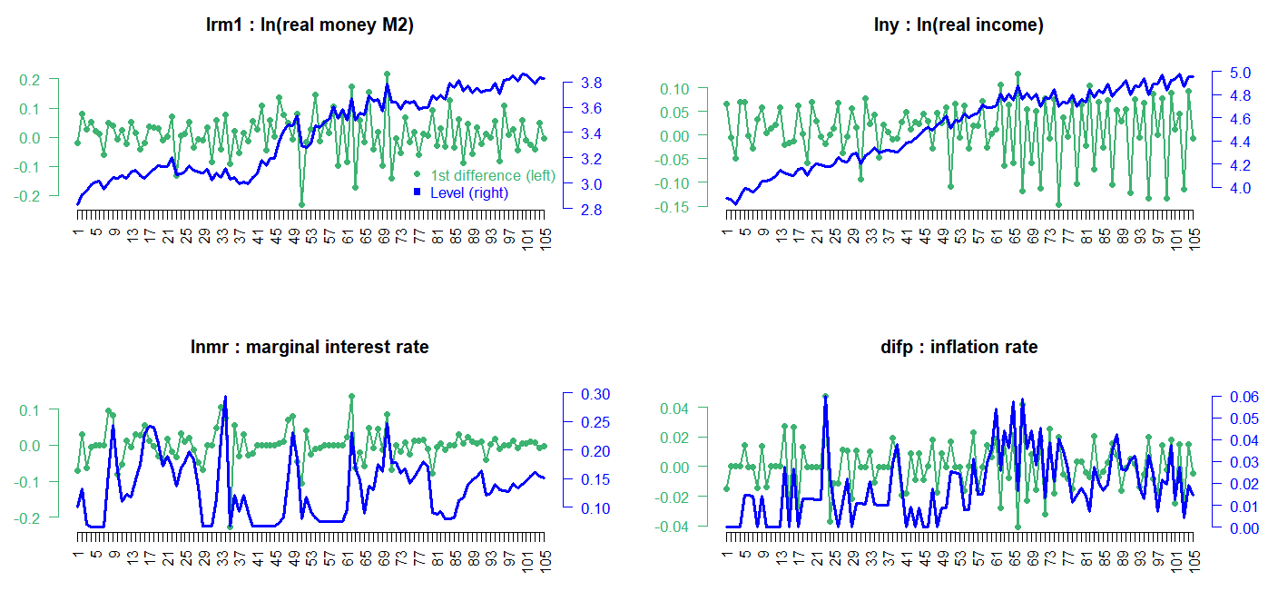
Visual inspections of this data in level show that real income rises, there is a demand for more money to make the transactions. On the other hand, the negative relationship between money and interest rate is found since the interest one gives up is the opportunity cost of holding money. To be consistent with the estimated results of Johansen and Juselius (1990), we set VECM lag = 1 (VAR lag = 2) and the quarterly demeaned seasonal dummy variables and ecdet = “none” in ca.jo() function or LRinclude = “none” in VECM() function. For the Johansen cointegration test, we use maximum eigenvalue test (type = “eigen” in ca.jo() function)
R code
In the following R code, we set up VAR(p) model in levels and perform the Johansen cointegration test and estimate parameteres. With these estimated parameters, we forecast level variables.
|
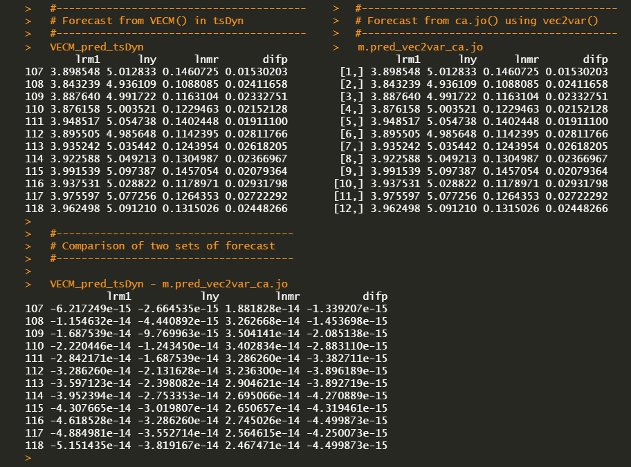
#========================================================# # Quantitative ALM, Financial Econometrics & Derivatives # ML/DL using R, Python, Tensorflow by Sang-Heon Lee # # https://kiandlee.blogspot.com #——————————————————–# # Vector Error Correction Model and Cointegration #========================================================# graphics.off() # clear all graphs rm(list = ls()) # remove all files from your workspace library(urca) # ca.jo, ur.df, finland library(vars) # vec2var library(tsDyn) # VECM #======================================================== # Data #======================================================== # level data : 1958q1 – 1984q2 data(finland) lev <– finland; nr_lev <– nrow(lev) # the sample period yq <– expand.grid(1:4, 1958:1984)[1:nr_lev,] colnames(yq) <– c(“q”, “yyyy”); rownames(yq) <– NULL # quarterly centered dummy variables yq$Q1 <– (yq$q==1)–1/4 yq$Q2 <– (yq$q==2)–1/4 yq$Q3 <– (yq$q==3)–1/4 dum_season <– yq[,–c(1,2)] # 1st differenced data dif <– as.data.frame(diff(as.matrix(lev), lag = 1)) #======================================================== # Cointegration Test #======================================================== #———————————————- # Johansen Cointegration Procedure #———————————————- # ecdet = ‘none’ for no intercept # ‘const’ for constant term # ‘trend’ for trend variable # in cointegration # type = eigen or trace test # K = lag order of VAR # spec = “transitory” or “longrun” # season = centered seasonal dummy (4:quarterly) # dumvar = another dummy variables #———————————————- coint_ca.jo <– ca.jo( lev, ecdet = “none”, type = “eigen”, K = 2, spec = “transitory”, season = 4, dumvar = NULL) summary(coint_ca.jo) #======================================================== # VECM model estimation #======================================================== #———————————————— # VECM estimation #———————————————— # VECM(data, lag, r = 1, # include = c(“const”, “trend”, “none”, “both”), # beta = NULL, estim = c(“2OLS”, “ML”), # LRinclude = c(“none”, “const”,”trend”, “both”), # exogen = NULL) #———————————————— VECM_tsDyn <– VECM(lev, lag=1, r=2, estim = “ML”, LRinclude = “none”, exogen = dum_season) #———————————————— # restricted VECM -> input for r #———————————————— cajorls_ca.jo <– cajorls(coint_ca.jo, r=2) #———————————————— # the VAR representation of a VECM from ca.jo #———————————————— # vec2var: Transform a VECM to VAR in levels # ca.jo is transformed to a VAR in level # r : The cointegration rank #———————————————— vec2var_ca.jo <– vec2var(coint_ca.jo, r=2) #======================================================== # Estimation Results #======================================================== #———————————————- # parameter estimates from each model #———————————————- VECM_tsDyn cajorls_ca.jo vec2var_ca.jo #======================================================== # Forecast #======================================================== # forecasting horizon nhor <– 12 #———————————————- # Forecast from VECM() in tsDyn #———————————————- # quarterly centered dummy variables for forecast dumf_season <– rbind(tail(dum_season,4), tail(dum_season,4), tail(dum_season,4)) VECM_pred_tsDyn <– predict(VECM_tsDyn, exoPred = dumf_season, n.ahead=nhor) # Draw Graph x11(width=8, height = 8); par(mfrow=c(4,1), mar=c(2,2,2,2)) # historical data + forecast data df <– rbind(lev, VECM_pred_tsDyn) for(i in 1:4) { matplot(df[,i], type=c(“l”), col = c(“blue”), main = str.main[i]) abline(v=nr_lev, col=“blue”) } VECM_pred_tsDyn #———————————————- # Forecast from ca.jo() using vec2var() #———————————————- pred_vec2var_ca.jo <– predict(vec2var_ca.jo, n.ahead=nhor) x11(); par(mai=rep(0.4, 4)); plot(pred_vec2var_ca.jo) x11(); par(mai=rep(0.4, 4)); fanchart(pred_vec2var_ca.jo) m.pred_vec2var_ca.jo <– cbind( pred_vec2var_ca.jo$fcst$lrm1[,1], pred_vec2var_ca.jo$fcst$lny[,1], pred_vec2var_ca.jo$fcst$lnmr[,1], pred_vec2var_ca.jo$fcst$difp[,1]) colnames(m.pred_vec2var_ca.jo) <– colnames(lev) m.pred_vec2var_ca.jo #———————————————- # Comparison of two sets of forecast #———————————————- VECM_pred_tsDyn – m.pred_vec2var_ca.jo |
cs |
Three models generate the same estimated parameters. Using these parameters we forecast the future values of the endogenous variables. However, cajorls() function can not be inserted into the predict() function. Therefore,
Results of Cointegration Test
summary(coint_ca.jo) delivers the following maximum eigenvalue cointegration test results with (beta) and (alpha) estimates.
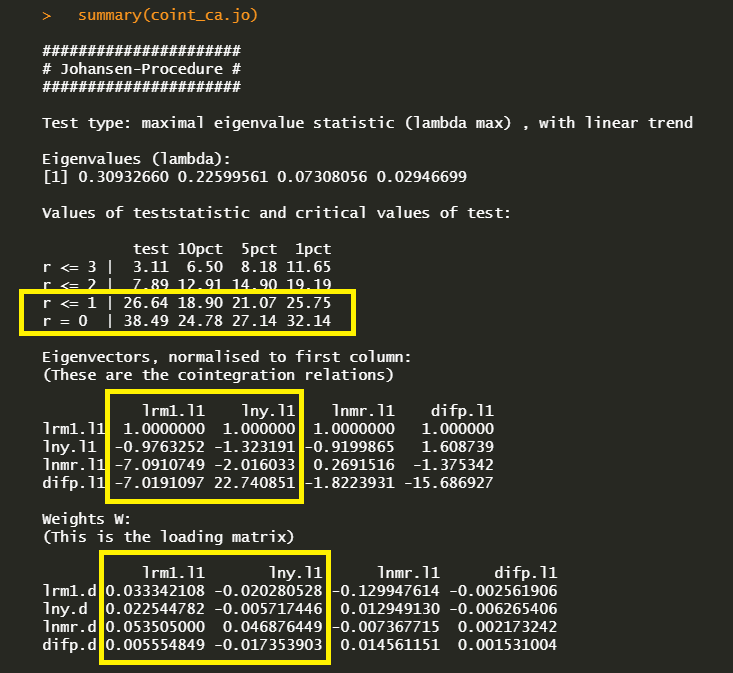
In the first r = 0 null hypothesis, since the test statistic 33.49 exceeds the 1, 5 and 10% critical values, there is at least one cointegration. In the second r = 1 null hypothesis, since the test statistic 26.64 also exceed the all critical values, the second hypothesis rejected. But in the third r = 3 null hypothesis, since the test statistic 7.89 does not exceed the all critical values, the third hypothesis can not be rejected. Therefore the cointegration is found at r = 2 under the maximum eigenvalue statistics.
Estimation Results
We estimate VECM parameters using three methods the following estimated results show the same output.


It seems that the following vec2var() output is different with the above two outputs. It’s because vec2var() estimate not a VECM in differences but a VAR in levels.

In particular, the first (VECM()) and second output(cajorls()) estimate beta coefficients with zero restrictions on some parameters. It is because of the fact that the eigenvector matrix is normalized using the Phillips triangular representation, which is used for identifying the relationships by using one zero restrictions (because we have two cointegrating relations r-1) in each relation. For this reason, we can see the shape of identity matrix from the upper position of estimated beta matrix.
Forecasting Results
Unlike a vec2var() object with the ca.jo() output and VECM() object in tsDyn, cajorls() object is not linked to the prediction functionality. For this reason we need to perform a forecast of the VECM model by using the aforementioned two methods. Since forecast figures from two methods are same, we can use either one method.
The following figures is from the VECM() function in the tsDyn.
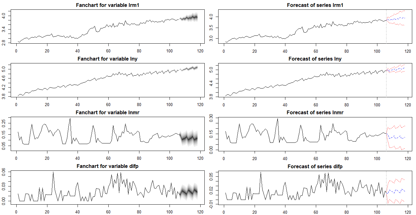
The following figure is from the vec2var() function in the vars with the ca.jo() result.

The differences between two forecast results are numerically zero at each point in forecasting horizon.
Concluding Remarks
In this post, we’ve implemented R code for the estimation of VECM model using several useful R package. The area of cointegration or VECM is so vast that it is difficult for me to understand it exactly. Nevertheless, I try to make clear explanations regarding some confusing parts in the VECM modeling. There are some interesting issues in this area such as the weak exogeneity restrictions or user defined cointegrating relationships based on some economic theory. This will be discussed later.
Reference
Johansen, S. and Juselius, K. (1990), Maximum Likelihood Estimation and Inference on Cointegration – with Applications to the Demand for Money, Oxford Bulletin of Economics and Statistics, 52, 2, 169–210. (blacksquare)
Time Series: Nonstationarity
rm(list=ls()) #Removes all items in Environment!
library(tseries) # for ADF unit root tests
library(dynlm)
library(nlWaldTest) # for the `nlWaldtest()` function
library(lmtest) #for `coeftest()` and `bptest()`.
library(broom) #for `glance(`) and `tidy()`
library(PoEdata) #for PoE4 datasets
library(car) #for `hccm()` robust standard errors
library(sandwich)
library(knitr) #for kable()
library(forecast)
New package: tseries (Trapletti and Hornik 2016).
A time series is nonstationary if its distribution, in particular its mean, variance, or timewise covariance change over time. Nonstationary time series cannot be used in regression models because they may create spurious regression, a false relationship due to, for instance, a common trend in otherwise unrelated variables. Two or more nonstationary series can still be part of a regression model if they are cointegrated, that is, they are in a stationary relationship of some sort.
We are concerned with testing time series for nonstationarity and finding out how can we transform nonstationary time series such that we can still use them in regression analysis.
data("usa", package="PoEdata")
usa.ts <- ts(usa, start=c(1984,1), end=c(2009,4),
               frequency=4)
Dgdp <- diff(usa.ts[,1])
Dinf <- diff(usa.ts[,"inf"])
Df <- diff(usa.ts[,"f"])
Db <- diff(usa.ts[,"b"])
usa.ts.df <- ts.union(gdp=usa.ts[,1], # package tseries
                      inf=usa.ts[,2],
                      f=usa.ts[,3],
                      b=usa.ts[,4],
                      Dgdp,Dinf,Df,Db,
                      dframe=TRUE)

plot(usa.ts.df$gdp)
plot(usa.ts.df$Dgdp)
plot(usa.ts.df$inf)
plot(usa.ts.df$Dinf)
plot(usa.ts.df$f)
plot(usa.ts.df$Df)
plot(usa.ts.df$b)
plot(usa.ts.df$Db)
A novelty in the above code sequence is the use of the function ts.union, wich binds together several time series, with the possibility of constructing a data frame. Table 12.1 presents the head of this data frame.
kable(head(usa.ts.df),
caption="Time series data frame constructed with 'ts.union'")| gdp | inf | f | b | Dgdp | Dinf | Df | Db |
|---|---|---|---|---|---|---|---|
| 3807.4 | 9.47 | 9.69 | 11.19 | NA | NA | NA | NA |
| 3906.3 | 10.03 | 10.56 | 12.64 | 98.9 | 0.56 | 0.87 | 1.45 |
| 3976.0 | 10.83 | 11.39 | 12.64 | 69.7 | 0.80 | 0.83 | 0.00 |
| 4034.0 | 11.51 | 9.27 | 11.10 | 58.0 | 0.68 | -2.12 | -1.54 |
| 4117.2 | 10.51 | 8.48 | 10.68 | 83.2 | -1.00 | -0.79 | -0.42 |
| 4175.7 | 9.24 | 7.92 | 9.76 | 58.5 | -1.27 | -0.56 | -0.92 |
AR(1), the First-Order Autoregressive Model
An AR(1) stochastic process is defined by Equation ref{eq:ar1def12}, where the error term is sometimes called “innovation” or “shock.”
[begin{equation}
y_{t}=rho y_{t-1}+nu_{t},;;;|rho |<1
label{eq:ar1def12}
end{equation}]
The AR(1) process is stationary if (| rho | <1); when (rho=1), the process is called random walk. The next code piece plots various AR(1) processes, with or without a constant, with or without trend (time as a term in the random process equation), with (rho) lesss or equal to 1. The generic equation used to draw the diagrams is given in Equation ref{eq:ar1generic12}.
[begin{equation}
y_{t}=alpha+lambda t+rho y_{t-1}+nu_{t}
label{eq:ar1generic12}
end{equation}]
N <- 500
a <- 1
l <- 0.01
rho <- 0.7

set.seed(246810)
v <- ts(rnorm(N,0,1))

y <- ts(rep(0,N))
for (t in 2:N){
  y[t]<- rho*y[t-1]+v[t]
}
plot(y,type='l', ylab="rho*y[t-1]+v[t]")
abline(h=0)

y <- ts(rep(0,N))
for (t in 2:N){
  y[t]<- a+rho*y[t-1]+v[t]
}
plot(y,type='l', ylab="a+rho*y[t-1]+v[t]")
abline(h=0)

y <- ts(rep(0,N))
for (t in 2:N){
  y[t]<- a+l*time(y)[t]+rho*y[t-1]+v[t]
}
plot(y,type='l', ylab="a+l*time(y)[t]+rho*y[t-1]+v[t]")
abline(h=0)

y <- ts(rep(0,N))
for (t in 2:N){
  y[t]<- y[t-1]+v[t]
}
plot(y,type='l', ylab="y[t-1]+v[t]")
abline(h=0)

a <- 0.1
y <- ts(rep(0,N))
for (t in 2:N){
  y[t]<- a+y[t-1]+v[t]
}
plot(y,type='l', ylab="a+y[t-1]+v[t]")
abline(h=0)

y <- ts(rep(0,N))
for (t in 2:N){
  y[t]<- a+l*time(y)[t]+y[t-1]+v[t]
}
plot(y,type='l', ylab="a+l*time(y)[t]+y[t-1]+v[t]")
abline(h=0)
Spurious Regression
Nonstationarity can lead to spurious regression, an apparent relationship between variables that are, in reality not related. The following code sequence generates two independent random walk processes, (y) and (x), and regresses (y) on (x).
T <- 1000
set.seed(1357)
y <- ts(rep(0,T))
vy <- ts(rnorm(T))
for (t in 2:T){
  y[t] <- y[t-1]+vy[t]
}

set.seed(4365)
x <- ts(rep(0,T))
vx <- ts(rnorm(T))
for (t in 2:T){
  x[t] <- x[t-1]+vx[t]
}
y <- ts(y[300:1000])
x <- ts(x[300:1000])
ts.plot(y,x, ylab="y and x")
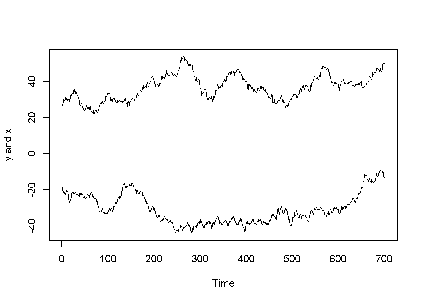
Figure 12.3: Artificially generated independent random variables
spurious.ols <- lm(y~x)
summary(spurious.ols)
##
## Call:
## lm(formula = y ~ x)
##
## Residuals:
## Min 1Q Median 3Q Max
## -12.55 -5.97 -2.45 4.51 24.68
##
## Coefficients:
## Estimate Std. Error t value Pr(>|t|)
## (Intercept) -20.3871 1.6196 -12.59 < 2e-16 ***
## x -0.2819 0.0433 -6.51 1.5e-10 ***
## ---
## Signif. codes: 0 '***' 0.001 '**' 0.01 '*' 0.05 '.' 0.1 ' ' 1
##
## Residual standard error: 7.95 on 699 degrees of freedom
## Multiple R-squared: 0.0571, Adjusted R-squared: 0.0558
## F-statistic: 42.4 on 1 and 699 DF, p-value: 1.45e-10The summary output of the regression shows a strong correlation between the two variables, thugh they have been generated independently. (Not any two randomly generated processes need to create spurious regression, though.) Figure 12.3 depicts the two time series, (y) and (x), and Figure 12.4 shows them in a scatterplot.
plot(x, y, type="p", col="grey")
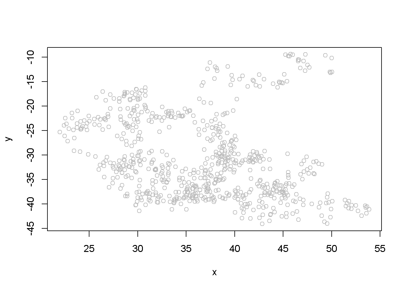
Figure 12.4: Scatter plot of artificial series y and x
Unit Root Tests for Stationarity
The Dickey-Fuller test for stationarity is based on an AR(1) process as defined in Equation ref{eq:ar1def12}; if our time series seems to display a constant and trend, the basic equation is the one in Equation ref{eq:ar1generic12}. According to the Dickey-Fuller test, a time series is nonstationary when (rho=1), which makes the AR(1) process a random walk. The null and alternative hypotheses of the test is given in Equation ref{eq:hypdftest12}.
[begin{equation}
H_{0}: rho=1, ;;; H_{A}: rho <1
label{eq:hypdftest12}
end{equation}]
The basic AR(1) equations mentioned above are transformed, for the purpose of the DF test into Equation ref{eq:dftesteqn12}, with the transformed hypothesis shown in Equation ref{eq:dftesthypo12}. Rejecting the DF null hypothesis implies that our time series is stationary.
[begin{equation}
Delta y_{t}=alpha+gamma y_{t-1}+lambda t +nu_{t}
label{eq:dftesteqn12}
end{equation}]
[begin{equation}
H_{0}: gamma =0, ;;;H_{A}: gamma <0
label{eq:dftesthypo12}
end{equation}]
An augmented DF test includes several lags of the variable tested; the number of lags to include can be assessed by examining the correlogram of the variable. The DF test can be of three types: with no constant and no trend, with constsnt and no trend, and, finally, with constant and trend. It is important to specify which DF test we want because the critical values are different for the three different types of the test. One decides which test to perform by examining a time series plot of the variable and determine if an imaginary regression line would have an intercept and a slope.
Let us apply the DF test to the (f) series in the (usa) dataset.
plot(usa.ts.df$f)
Acf(usa.ts.df$f)
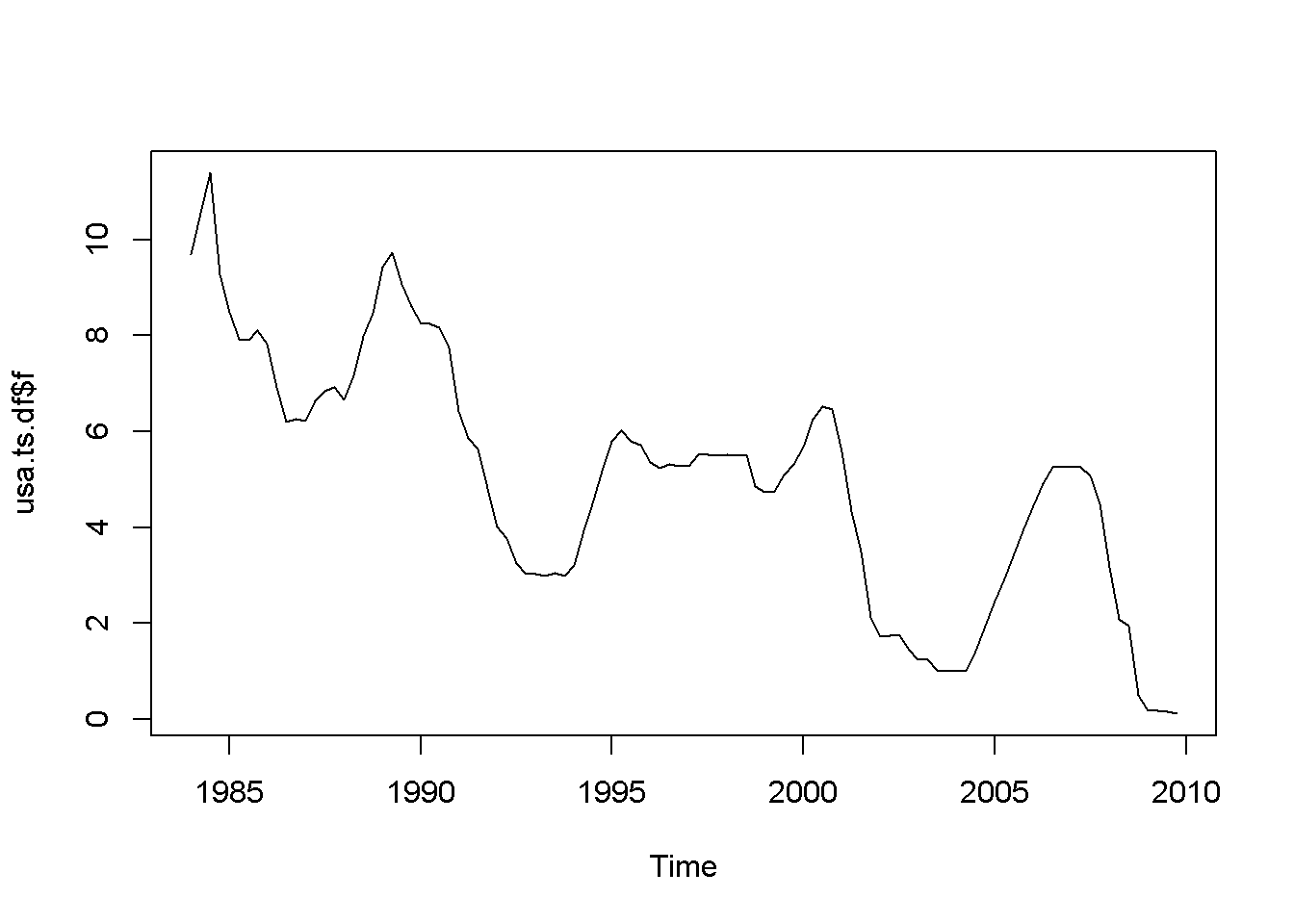
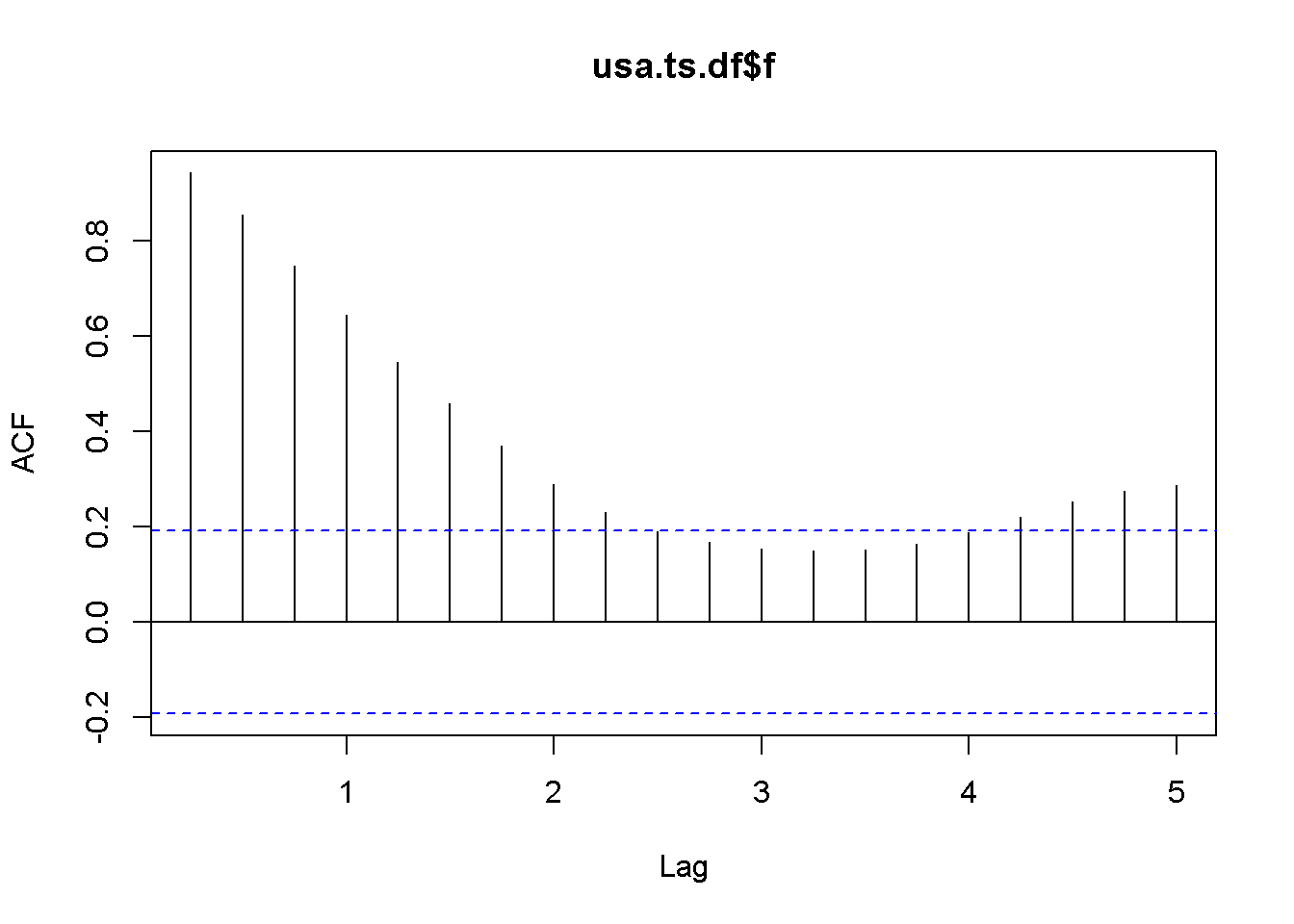
Figure 12.5: A plot and correlogram for series f in dataset usa
The time series plot in Figure 12.5 indicates both intercept and trend for our series, while the correlogram suggests including 10 lags in the DF test equation. Suppose we choose (alpha=0.05) for the DF test. The adf.test function does not require specifying whether the test should be conducted with constant or trend, and if no value for the number of lags is given (the argument for the number of lags is k), (R) will calculate a value for it. I would recommend always taking a look at the series’ plot and correlogram.
adf.test(usa.ts.df$f, k=10)##
## Augmented Dickey-Fuller Test
##
## data: usa.ts.df$f
## Dickey-Fuller = -3.373, Lag order = 10, p-value = 0.0628
## alternative hypothesis: stationaryThe result of the test is a (p)-value greater than our chosen significance level of 0.05; therefore, we cannot reject the null hypothesis of nonstationarity.
adf.test(usa.ts.df$b, k=10)##
## Augmented Dickey-Fuller Test
##
## data: usa.ts.df$b
## Dickey-Fuller = -2.984, Lag order = 10, p-value = 0.169
## alternative hypothesis: stationaryHere is a code to reproduce the results in the textbook.
f <- usa.ts.df$f
f.dyn <- dynlm(d(f)~L(f)+L(d(f)))
tidy(f.dyn)| term | estimate | std.error | statistic | p.value |
|---|---|---|---|---|
| (Intercept) | 0.172522 | 0.100233 | 1.72121 | 0.088337 |
| L(f) | -0.044621 | 0.017814 | -2.50482 | 0.013884 |
| L(d(f)) | 0.561058 | 0.080983 | 6.92812 | 0.000000 |
b <- usa.ts.df$b
b.dyn <- dynlm(d(b)~L(b)+L(d(b)))
tidy(b.dyn)| term | estimate | std.error | statistic | p.value |
|---|---|---|---|---|
| (Intercept) | 0.236873 | 0.129173 | 1.83376 | 0.069693 |
| L(b) | -0.056241 | 0.020808 | -2.70285 | 0.008091 |
| L(d(b)) | 0.290308 | 0.089607 | 3.23979 | 0.001629 |
A concept that is closely related to stationarity is order of integration, which is how many times we need to difference a series untill it becomes stationary. A series is I(0), that is, integrated of order (0) if it is already stationary (it is stationary in levels, not in differences); a series is I(1) if it is nonstationary in levels, but stationary in its first differences.
df <- diff(usa.ts.df$f)
plot(df)
Acf(df)
adf.test(df, k=2)
##
## Augmented Dickey-Fuller Test
##
## data: df
## Dickey-Fuller = -4.178, Lag order = 2, p-value = 0.01
## alternative hypothesis: stationary
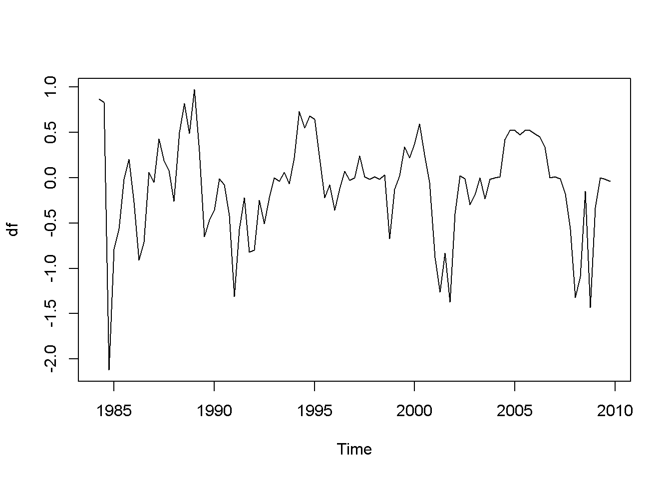
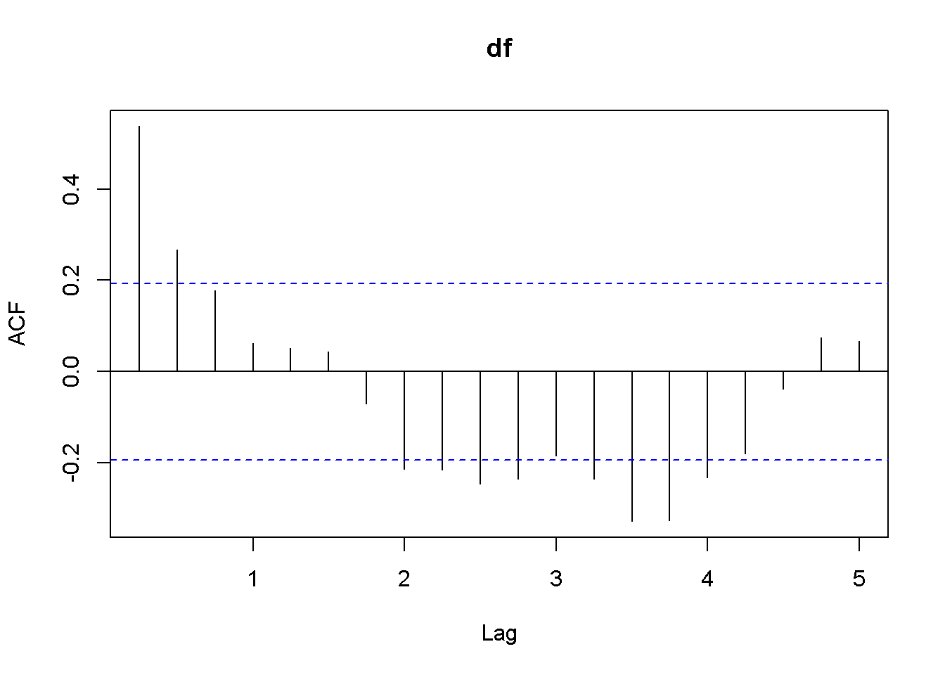
Figure 12.6: Plot and correlogram for series diff(f) in dataset usa
db <- diff(usa.ts.df$b)
plot(db)
Acf(db)
adf.test(db, k=1)
##
## Augmented Dickey-Fuller Test
##
## data: db
## Dickey-Fuller = -6.713, Lag order = 1, p-value = 0.01
## alternative hypothesis: stationary
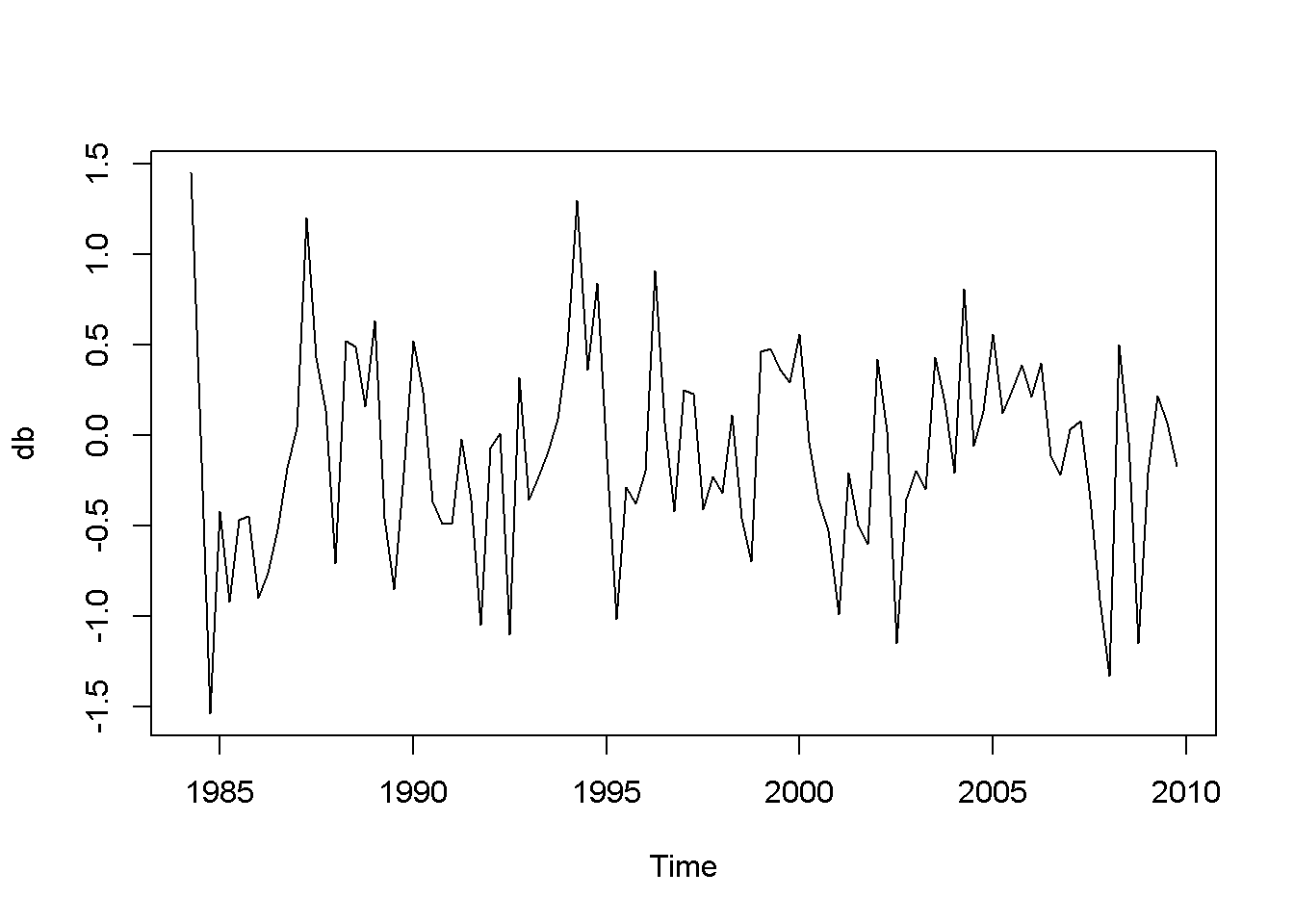
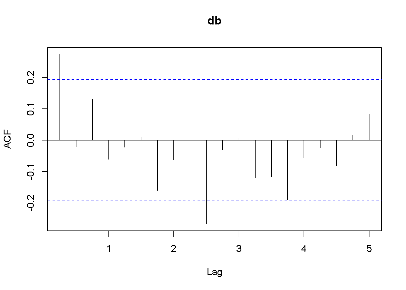
Figure 12.7: Plot and correlogram for series diff(b) in dataset usa
Both the plots and the DF tests indicate that the (f) and (b) series are stationary in first differences, which makes each of them integrated of order 1. The next code sequence reproduces the results in the textbook. Please note the term ((-1)) in the dynlm command; it tells (R) that we do not want an intercept in our model. Figures 12.6 and 12.7 show plots of the differenced (f) and (b) series, respectively.
df.dyn <- dynlm(d(df)~L(df)-1)
db.dyn <- dynlm(d(db)~L(db)-1)
tidy(df.dyn)| term | estimate | std.error | statistic | p.value |
|---|---|---|---|---|
| L(df) | -0.446986 | 0.081462 | -5.48706 | 0 |
| term | estimate | std.error | statistic | p.value |
|---|---|---|---|---|
| L(db) | -0.701796 | 0.091594 | -7.66205 | 0 |
Function ndiffs() in the package forecast is a very convenient way of determining the order of integration of a series. The arguments of this function are x, a time series, alpha, the significacnce level of the test (0.05 by default), test= one of “kpss”, “adf”, or “pp”, which indicates the unit root test to be used; we have only studied the “adf” test.), and max.d= maximum number of differences. The output of this function is an integer, which is the order of integration of the time series.
## [1] 1## [1] 1As we have already found, the orders of integration for both (f) and (b) are 1.
Cointegration
Two series are cointegrated when their trends are not too far apart and are in some sense similar. This vague statement, though, can be made precise by conducting a cointegration test, which tests whether the residuals from regressing one series on the other one are stationary. If they are, the series are cointegrated. Thus, a cointegration test is in fact a Dickey-Fuler stationarity test on residuals, and its null hypothesis is of noncointegration. In other words, we would like to reject the null hypothesis in a cointegration test, as we wanted in a stationarity test.
Let us apply this method to determine the state of cointegration between the series (f) and (b) in dataset (usa).
fb.dyn <- dynlm(b~f)
ehat.fb <- resid(fb.dyn)
ndiffs(ehat.fb) #result: 1
## [1] 1output <- dynlm(d(ehat.fb)~L(ehat.fb)+L(d(ehat.fb))-1) #no constant
foo <- tidy(output)
foo| term | estimate | std.error | statistic | p.value |
|---|---|---|---|---|
| L(ehat.fb) | -0.224509 | 0.053504 | -4.19613 | 0.000059 |
| L(d(ehat.fb)) | 0.254045 | 0.093701 | 2.71124 | 0.007891 |
The relevant statistic is (tau = -4.196133), which is less than (-3.37), the relevant critical value for the cointegration test. In conclusion, we reject the null hypothesis that the residuals have unit roots, therefore the series are cointegrated.
(R) has a special function to perform cointegration tests, function po.test in package tseries. (The name comes from the method it uses, which is called “Phillips-Ouliaris.”) The main argument of the function is a matrix having in its first column the dependent variable of the cointegration equation and the independent variables in the other columns. Let me illustrate its application in the case of the same series (fb) and (f).
bfx <- as.matrix(cbind(b,f), demean=FALSE)
po.test(bfx)
##
## Phillips-Ouliaris Cointegration Test
##
## data: bfx
## Phillips-Ouliaris demeaned = -20.51, Truncation lag parameter = 1,
## p-value = 0.0499The PO test marginally rejects the null of no cointegration at the 5 percent level.
The Error Correction Model
A relationship between cointegrated I(1) variables is a long run relationship, while a relationship between I(0) variables is a short run one. The short run error correction model combines, in some sense, short run and long run effects. Starting from an ARDL(1,1) model (Equation ref{eq:ardl11error12}) and assuming that there is a steady state (long run) relationship between (y) and (x), one can derive the error correction model in Equation ref{eq:errorcorreqn12}, where more lagged differences of (x) may be necessary to eliminate autocorrelation.
[begin{equation}
y_{t}=delta+theta_{1}y_{t-1}+delta_{0}x_{t}+delta_{1}x_{t-1}+nu_{t}
label{eq:ardl11error12}
end{equation}]
[begin{equation}
Delta y_{t}=-alpha (y_{t-1}-beta_{1}-beta_{2}x_{t-1})+delta_{0}Delta x_{t}+nu_{t}
label{eq:errorcorreqn12}
end{equation}]
In the case of the US bonds and funds example, the error correction model can be constructed as in Equation ref{eq:bferrorcorrection12}.
[begin{equation}
Delta b_{t}=-alpha (b_{t-1}-beta_{1}-beta_{2}f_{t-1})+delta_{0}Delta , f_{t}+ delta_{1}Delta , f_{t-1} + nu_{t}
label{eq:bferrorcorrection12}
end{equation}]
The (R) function that estimates a nonlinear model such as the one in Equation ref{eq:bferrorcorrection12} is nls, which requires three main argumants: a formula, which is the regression model to be estimated written using regular text mathematical operators, a start= list of guessed or otherwise approximated values of the estimated parameters to initiate a Gauss-Newton numerical optimization process, and data= a data frame, list, or environment data source. Please note that data cannot be a matrix.
In the next code sequence, the initial values of the parameters have been determined by estimating Equation ref{eq:ardl11error12} with (b) and (f) replacing (y) and (x).
b.ols <- dynlm(L(b)~L(f))
b1ini <- coef(b.ols)[[1]]
b2ini <- coef(b.ols)[[2]]
d.ols <- dynlm(b~L(b)+f+L(f))
aini <- 1-coef(d.ols)[[2]]
d0ini <- coef(d.ols)[[3]]
d1ini <- coef(d.ols)[[4]]
Db <- diff(b)
Df <- diff(f)
Lb <- lag(b,-1)
Lf <- lag(f,-1)
LDf <- lag(diff(f),-1)
bfset <- data.frame(ts.union(cbind(b,f,Lb,Lf,Db,Df,LDf)))
formula <- Db ~ -a*(Lb-b1-b2*Lf)+d0*Df+d1*LDf
bf.nls <- nls(formula, na.action=na.omit, data=bfset,
          start=list(a=aini, b1=b1ini, b2=b2ini,
                     d0=d0ini, d1=d1ini))
kable(tidy(bf.nls),
caption="Parameter estimates in the error correction model")| term | estimate | std.error | statistic | p.value |
|---|---|---|---|---|
| a | 0.141877 | 0.049656 | 2.85720 | 0.005230 |
| b1 | 1.429188 | 0.624625 | 2.28807 | 0.024304 |
| b2 | 0.776557 | 0.122475 | 6.34052 | 0.000000 |
| d0 | 0.842463 | 0.089748 | 9.38697 | 0.000000 |
| d1 | -0.326845 | 0.084793 | -3.85463 | 0.000208 |
The error correction model can also be used to test the two series for cointegration. All we need to do is to test the errors of the correction part embedded in Equation ref{eq:bferrorcorrection12} for stationarity. The estimated errors are given by Equation ref{eq:embederrors12}.
[begin{equation}
hat{e}_{t-1}=b_{t-1}-beta_{1}-beta_{2}f_{t-1}
label{eq:embederrors12}
end{equation}]
ehat <- bfset$Lb-coef(bf.nls)[[2]]-coef(bf.nls)[[3]]*bfset$Lf
ehat <- ts(ehat)
ehat.adf <- dynlm(d(ehat)~L(ehat)+L(d(ehat))-1)
kable(tidy(ehat.adf),
caption="Stationarity test within the error correction model")| term | estimate | std.error | statistic | p.value |
|---|---|---|---|---|
| L(ehat) | -0.168488 | 0.042909 | -3.92668 | 0.000158 |
| L(d(ehat)) | 0.179486 | 0.092447 | 1.94149 | 0.055013 |
To test for cointegration, one should compare the (t)-ratio of the lagged term shown as ‘statistic’ in Equation 12.3, (t=-3.927) to the critical value of (-3.37). The result is to reject the null of no cointegration, which means the series are cointegrated.
References
I have to estimate the relationship between prices in New York(N) and London(L) using a vector error correction model adapted from Joel Hasbrouck. After much research online, I still have not made much headway so I thought that I would ask you experts to see if I can get some direction in getting this model done.
My dataset is a dataframe with date, time, symbol, price.
Return(r_t) is defined as the log difference between price for each fifteen minute interval (p(t) — p(t-1)) for both New York and London (equation 1 and 2).
The model uses r_t in New York to model on 2 lags of returns in new york and London (equation 3).
Then uses in r-t in London to model on 2 lags of returns in new york and london (equation 4).
N and L represent New York and London respectively anywhere seen in the model and t represents time.
r_t^N=∆ log(P_t^N )
r_t^L=∆ log(P_t^L )
r_t^N=α(log(P_(t-1)^N)-log(P_(t-1)^L))+∑_(i=1)to 2(γ_i^(N,N) r_(t-i)^N) + ∑_(i=1)to 2(γ_i^(N,L) r_(t-i)^L)+ ε_t^N
r_t^L=α(log(P_(t-1)^L)-log(P_(t-1)^N))+∑_(i=1)to 2(γ_i^(L,L) r_(t-i)^L) + ∑_(i=1)to 2(γ_i^(L,N) r_(t-i)^N)+ ε_t^L
Any help will be soooooo appreciated. Thank you in advance for your help!!
I am new to R and have a bit more experience using SAS and the time series procedures there. I have seen reference to using vars() but the examples I have looked at do not seem applicable so I am pretty much stuck. I have done the DW statistic and there is co-integration.
I just can’t figure out how to write the code for this …
ecm: Error Correction Model
Description
Fits an error correction model for univriate response.
Usage
ecm(y, X, output = TRUE)
Arguments
y
a response of a numeric vector or univariate time series.
X
an exogenous input of a numeric vector or a matrix for multivariate time series.
output
a logical value indicating to print the results in R console.
The default is TRUE.
Value
- An object with class «
lm«, which is the same results oflmfor
fitting linear regression.
Details
An error correction model captures the short term relationship between the
response y and the exogenous input variable X. The model is defined as
$$dy[t] = bold{beta}[0]*dX[t] + beta[1]*ECM[t-1] + e[t],$$
where $d$ is an operator of the first order difference, i.e.,
$dy[t] = y[t] — y[t-1]$, and $bold{beta}[0]$ is a coefficient vector with the
number of elements being the number of columns of X (i.e., the number
of exogenous input variables), and$ECM[t-1] = y[t-1] — hat{y}[t-1]$ which is the
main term in the sense that its coefficient $beta[1]$ explains the short term
dynamic relationship between y and X
in this model, in which $hat{y}[t]$ is estimated from the linear regression model
$y[t] = bold{alpha}*X[t] + u[t]$. Here, $e[t]$ and $u[t]$ are both error terms
but from different linear models.
References
Engle, Robert F.; Granger, Clive W. J. (1987). Co-integration and error correction:
Representation, estimation and testing. Econometrica, 55 (2): 251-276.
Examples
Run this code
X <- matrix(rnorm(200),100,2)
y <- 0.1*X[,1] + 2*X[,2] + rnorm(100)
ecm(y,X)
Run the code above in your browser using DataCamp Workspace
Description
Usage
Arguments
Details
Value
See Also
Examples
Builds an lm object that represents an error correction model (ECM) by automatically differencing and
lagging predictor variables according to ECM methodology.
y |
The target variable |
xeq |
The variables to be used in the equilibrium term of the error correction model |
xtr |
The variables to be used in the transient term of the error correction model |
lags |
The number of lags to use |
includeIntercept |
Boolean whether the y-intercept should be included (should be set to TRUE if using ‘earth’ as linearFitter) |
weights |
Optional vector of weights to be passed to the fitting process |
linearFitter |
Whether to use ‘lm’ or ‘earth’ to fit the model |
... |
Additional arguments to be passed to the ‘lm’ or ‘earth’ function (careful that some arguments may not be appropriate for ecm!) |
The general format of an ECM is
Δ y_{t} = β_{0} + β_{1}Δ x_{1,t} +…+ β_{i}Δ x_{i,t} + γ(y_{t-1} — (α_{1}x_{1,t-1} +…+ α_{i}x_{i,t-1})).
The ecm function here modifies the equation to the following:
Δ y = β_{0} + β_{1}Δ x_{1,t} +…+ β_{i}Δ x_{i,t} + γ y_{t-1} + γ_{1}x_{1,t-1} +…+ γ_{i}x_{i,t-1},
where γ_{i} = -γ α_{i},
so it can be modeled as a simpler ordinary least squares (OLS) function using R’s lm function.
Ordinarily, the ECM uses lag=1 when differencing the transient term and lagging the equilibrium term, as specified in the equation above. However, the ecm function here gives the user the ability to specify a lag greater than 1.
Notice that an ECM models the change in the target variable (y). This means that the predictors will be lagged and differenced,
and the model will be built on one observation less than what the user inputs for y, xeq, and xtr. If these arguments contain vectors with too few observations (eg. one single observation),
the function will not work. Additionally, for the same reason, if using weights in the ecm function, the length of weights should be one less than the number of rows in xeq or xtr.
When inputting a single variable for xeq or xtr in base R, it is important to input it in the format «xeq=df[‘col1’]» so they inherit the class ‘data.frame’. Inputting such as «xeq=df[,’col1′]» or «xeq=df$col1» will result in errors in the ecm function. You can load data via other R packages that store data in other formats, as long as those formats also inherit the ‘data.frame’ class.
By default, base R’s ‘lm’ is used to fit the model. However, users can opt to use ‘earth’, which uses Jerome Friedman’s Multivariate Adaptive Regression Splines (MARS) to build a regression model, which transforms each continuous variable into piece-wise linear hinge functions. This allows for non-linear features in both the transient and equilibrium terms.
ECM models are used for time series data. This means the user may need to consider stationarity and/or cointegration before using the model.
an lm object representing an error correction model
lm, earth
1 2 3 4 5 6 7 8 9 10 11 12 13 14 15 16 17 18 19 20 21 22 23 24 25 26 27 28 29 30 31 32 33 34 |
##Not run #Use ecm to predict Wilshire 5000 index based on corporate profits, #Federal Reserve funds rate, and unemployment rate. data(Wilshire) #Use 2015-12-01 and earlier data to build models trn <- Wilshire[Wilshire$date<='2015-12-01',] #Assume all predictors are needed in the equilibrium and transient terms of ecm. xeq <- xtr <- trn[c('CorpProfits', 'FedFundsRate', 'UnempRate')] model1 <- ecm(trn$Wilshire5000, xeq, xtr, includeIntercept=TRUE) #Assume CorpProfits and FedFundsRate are in the equilibrium term, #UnempRate has only transient impacts. xeq <- trn[c('CorpProfits', 'FedFundsRate')] xtr <- trn['UnempRate'] model2 <- ecm(trn$Wilshire5000, xeq, xtr, includeIntercept=TRUE) #From a strictly statistical standpoint, Wilshire data may not be stationary #and hence model1 and model2 may have heteroskedasticity in the residuals. #Let's check for that. lmtest::bptest(model1) lmtest::bptest(model2) #The Breush-Pagan tests suggest we should reject homoskedasticity in the residuals for both models. lmtest::bgtest(model1) lmtest::bgtest(model2) #The Breusch-Godfrey tests suggest we should reject that there is no serial correlation #in the residuals. #Given the above issues, see adjusted std. errors and p-values for our models. lmtest::coeftest(model1, vcov=sandwich::NeweyWest) lmtest::coeftest(model2, vcov=sandwich::NeweyWest) |
ecm documentation built on May 28, 2021, 5:07 p.m.