bug #31070: fzero cannot compute initial bracketing
| Submitter: | Carlo de Falco <cdf> | ||
| Submitted: | Sun 19 Sep 2010 12:24:28 PM UTC | ||
| Category: | Libraries | Severity: | 1 — Wish |
| Priority: | 3 — Low | Item Group: | Feature Request |
| Status: | Postponed | Assigned to: | highegg |
| Originator Name: | Open/Closed: * | Closed | |
| Release: * | dev | Operating System: * | Mac OS |
| Fixed Release: | None | Planned Release: | None |
* Mandatory Fields
Add a New Comment (![]() Rich Markup)
Rich Markup)
Comment Type & Canned Response:
|
Mon 20 Sep 2010 03:28:02 PM UTC, comment #3: I agree that this is not a bug, |
Carlo de Falco <cdf> |
|
Mon 20 Sep 2010 06:07:01 AM UTC, comment #2: |
Jaroslav Hajek <highegg> |
|
Sun 19 Sep 2010 11:23:12 PM UTC, comment #1: |
Carlo de Falco <cdf> |
|
Sun 19 Sep 2010 12:24:28 PM UTC, original submission: |
Carlo de Falco <cdf> |
(Note: upload size limit is set to 16384 kB, after insertion of
the required escape characters.)
Attach Files:
Comment:
Depends on the following items: None found
Items that depend on this one: None found
Carbon-Copy List
There are 0 votes so far. Votes easily highlight which items people would like to see resolved
in priority, independently of the priority of the item set by tracker
managers.
Only project members can vote.
Please enter the title of George Orwell’s famous
dystopian book (it’s a date):
![]()
7.2 Решение трансцендентных уравнений
Уравнение, в котором неизвестное входит в аргумент трансцендентных функций, называется трансцендентным уравнением. К трансцендентным уравнениям принадлежат показательные, логарифмические, тригонометрические.
Для решения трансцендентных уравнений вида  в Octave существует функция
  или
или ![fzero(name, [a, b])](https://intuit.ru/sites/default/files/tex_cache/5fff2a3e9373b95b078fec50acd24f67.png) , где
, где  — имя функции, вычисляющей левую часть уравнения,
  — начальное приближение к корню,
 ![[a, b]](https://intuit.ru/sites/default/files/tex_cache/022022f289db140169cd9514f74ee648.png) — интервал изоляции корня.
— интервал изоляции корня.
Если функция вызывается в формате: ![[x, y] = fzero(name, x0)](https://intuit.ru/sites/default/files/tex_cache/2562efaafed3bb64258ee94f5d6ac5c0.png) , то здесь
, то здесь  — корень уравнения,
  — значение функции в точке .
Пример 7.14. Найти решение уравнения:
![sqrt[3]{(2x-3)^2}- sqrt[3]{(x-1)^2}=0.](https://intuit.ru/sites/default/files/tex_cache/2797184839ebd07b7f8e224ba3830f7f.png)
Начнём решение данного трансцендентного уравнения с определения интервала изоляции корня. Воспользуемся для этого графическим методом. Построим график функции, указанной в левой части уравнения (листинг 7.15), создав предварительно функцию для её определения.
% Функция для вычисления левой части уравнения f(x)=0
function y=f1(x)
	y=((2-x-3).^2).^(1/3)-((x-1).^2).^(1/3);
end;
% Построение графика функции f(x)
cla; okno1=figure();
x = -1:0.1:3;
y=f1(x);
pol=plot(x, y);
set(pol, ’LineWidth’, 3, ’Color’, ’k’)
set(gca, ’xlim’, [-1, 3]); set(gca, ’ylim’, [-1,1.5]);
set(gca, ’xtick’, [-1:0.5:3]); set(gca, ’ytick’,[-1:0.5:1.5]);
grid on; xlabel(’x’); ylabel(’y’);
title(’Plot y=(2x-3)^{2/3}-(x-1)^{2/3}’);
Листинг
7.15.
Графическое отделение корней (пример 7.14).
На графике (рис. 7.3) видно, что функция  дважды пересекает ось
  . Первый раз на интервале [1, 1.5], второй — [1.5, 2.5].
Уточним корни, полученные графическим методом. Воспользуемся функцией, вычисляющей левую часть заданного уравнения из листинга 7.15 и обратимся к функции  , указав в качестве параметров имя созданной функции и число (1.5) близкое к первому корню:
>>> x1=fzero(’f1’, 1.5)
x1 = 1.3333
Теперь применим функцию , указав в качестве параметров имя функции, и интервал изоляции второго корня:
>>> x2=fzero(’f1’, [1.52.5])
x1= 2
Не трудно заметить, что и в первом и во втором случае функция правильно нашла корни заданного уравнения.

Рис.
7.3.
Графическое решение примера 7.14
Ниже приведён пример некорректного обращения к функции , здесь интервал изоляции корня задан неверно. На графике видно, что на концах этого интервала функция знак не меняет, или, другими словами, выбранный интервал содержит сразу два корня.
>>>fzero(’f1’, [1 3])
error: fzero: not a valid initial bracketing
error: called from:
error: /usr/share/octave/3.4.0/m/optimization/fzero.m at line 170, column 5
В следующем листинге приведён пример обращения к функции в полном формате:
>>> [X(1),Y(1)]= fzero(’f1’, [1 1.5]);
>>> [X(2),Y(2) ]= fzero(’f1’, [1.5 2.5]);
>>> X % Решение уравнения
X = 1.3333 2.0000
>>> Y % Значения функции в точке Х
Y = -2.3870e-15  0.0000e+00
Пример 7.15. Найти решение уравнения  .
.
Как видим, левая часть уравнения представляет собой полином. В примере 7.13 было показано, что данное уравнение имеет четыре корня: два действительных и два мнимых (листинг 7.14).
Листинг 7.16 демонстрирует решение алгебраического уравнения при помощи функции . Не трудно заметить, что результатом работы функции являются только действительные корни. Графическое решение (рис. 7.2) подтверждает это: функция дважды пересекает ось абсцисс.
function y=f2(x)
	y=x.^4+4-x.^3+4-x.^2-9;
end;
>>> [X(1),Y(1)]= fzero(’f2’, [-4 -2]);
>>> [X(2),Y(2)]= fzero(’f2’, [0 2]);
>>> X
>>> Y
X = -3 1
Y = 0 0
Листинг
7.16.
Решение уравнения с помощью fzero (пример 7.15).
![]()
-
Direct link to this question
⋮
-
Direct link to this question
Hi. So this is what I wrote so far in octave:
f=4*x.^2+20*x+4
f = ![]()
x=fzero(@(x) f, -5)
Error using fzero (line 308)
Initial function value must be finite and real.
but I keep getting the error in the title. What is wrong with what I wrote? Thanks in advance!
Answers (1)
![]()
-
Direct link to this answer
⋮
-
Direct link to this answer
Use fzero for numeric functions and solve for symbollic functions —
f=4*x.^2+20*x+4
f = ![]()
x=vpa(solve(f==0))
x =

xd = double(x)
xd = 2×1
-4.791287847477920
-0.208712152522080
whos x xd
Name Size Bytes Class Attributes
x 2×1 8 sym
xd 2×1 16 double
.
3 Comments
![]()
Direct link to this comment
⋮
-
Link
Direct link to this comment
How do I declare a numerical function?
![]()
Direct link to this comment
⋮
-
Link
Direct link to this comment
f=4*x.^2+20*x+4
f = ![]()
F = matlabFunction(f)
F = function_handle with value:
@(x)x.*2.0e+1+x.^2.*4.0+4.0
or
f = @(x) 4*x.^2 + 20*x + 4
f = function_handle with value:
@(x)4*x.^2+20*x+4
![]()
Direct link to this comment
⋮
-
Link
Direct link to this comment
One approach —
f=4*x.^2+20*x+4
f = ![]()
f_fcn = matlabFunction(f)
f_fcn = function_handle with value:
@(x)x.*2.0e+1+x.^2.*4.0+4.0
To get the other root, use a different initial parameter estimate —
.
Sign in to comment.
See Also
Categories
Community Treasure Hunt
Find the treasures in MATLAB Central and discover how the community can help you!
Start Hunting!
An Error Occurred
Unable to complete the action because of changes made to the page. Reload the page to see its updated state.
![]()
With Matlab, I obtained the plot below with the following simplified loop.
for i = 1:size(a0,2)
  fun3 = @(y) sind(90-y) - n*(sind(90-asind(sind(a0(i))/n)-y));
  y(i) = fzero(fun3, [0,90]);
end
The difference is in the form of equation: I replaced 90-y = asind(something) with sin(90-y) = something. When «something» is greater than 1 in absolute value, the former version throws an error due to complex value of asind. The latter proceeds normally, recognizing that this is not a solution (sin(90-y) can’t be equal to something that is greater than 1).
No precomputing of the bracket was necessary, [0,90] simply worked. Another change I made was in the plot: plot(a0,y) instead of plot(y), to get the correct horizontal axis.
And you can’t avoid for loop here, nor should you worry about it. Vectorization means eliminating loops where the content is a low-level operation that can be done en masse by operating on some C array. But fzero is totally not that. If the code takes long to run, it’s because solving a bunch of equations takes long, not because there’s a for loop.

The fzero command in MATLAB can be used to find the value of a single parameter of a multivariable function that will set the function equal to zero (if such a value exists). The command can only find one root at a time, and can only find roots in one variable at a time. There are several different ways to present fzero with the specific function and variable. In addition to the examples below, there is another page with more examples at MATLAB:Fzero/Examples.
Contents
- 1 Examples
- 1.1 Different Function Calls
- 1.1.1 Most General Case
- 1.1.1.1 Function on the Fly
- 1.1.1.2 Pre-Defined Functions
- 1.1.2 Single-Variable Anonymous Functions
- 1.1.3 Single-Variable Built-in Functions and .m Functions
- 1.1.1 Most General Case
- 1.2 Changing «Constant» Parameters
- 1.2.1 One Parameter
- 1.2.2 Two Parameters
- 1.1 Different Function Calls
- 2 Questions
- 3 External Links
- 4 References
Examples
Different Function Calls
Most General Case
The following examples show a method that will work regardless of how many input variables your function has or how you define your function — whether it is built-in, a variable containing an anonymous function, an anonymous function generated on the fly, or a .m file function. The paradigm is:
[ROOT, VAL_AT_ROOT] = fzero(@(DUMMY_VAR) FUNCTION_THING, INIT_STUFF, OPTIONS)
where
- ROOT is the calculated value of the requested variable when the function is 0
- VAL_AT_ROOT is the value of the function when substituting ROOT for the requested variable — nominally this is 0 but there may be roundoff issues to deal with
- DUMMY_VAR is the variable you want to use in this FUNCTION_THING to indicate which of the various inputs
fzerois allowed to alter - INIT_STUFF is either an initial guess or a valid initial bracket — note that
fzerocan only find one root at a time, so you cannot load this with several values and try to havefzerofind multiple results (for that, you need loops) - FUNCTION_THING can be a built-in function, the name of an anonymous function, the name of a .m file function, or a calculation — whatever it is that you are trying to set equal to zero; note that DUMMY_VAR must appear somewhere in this expression for
fzeroto be able to do anything - OPTIONS are…optional — the most common is the command
optimset('Display', 'iter')
if you want to see the magic happen
The example is based on wanting to determine roots of:
(f(x, y, z)=cos(x)+sin(y)+z=0,!)
We will assume that two of the three variables ((x) and (y)) are known and that we want to find (z) given those values. We will further assume that (x=1) and (y=pi). Finally, we will make an initial guess that (z=12).
Function on the Fly
If you only want to solve this problem once, and the calculation only requires one line of code, the process with the least «overhead» involves creating the function on the fly inside the fzero command. All you have to do is put your expression in for the FUNCTION_THING, making sure the DUMMY_VAR is appropriately used. The line:
[zValue, fValue] = fzero(@(zDummy) cos(1) + sin(pi) + zDummy, 12)
will produce
zValue =

  -5.4030e-01


fValue =

     0
A slightly «longer» version of this would have you pre-define the (x) and (y) variables first, then use the variables in the function definition:
expression in for the FUNCTION_THING, making sure the DUMMY_VAR is appropriately used. The line:
x = 1;
y = pi;
[zValue, fValue] = fzero(@(zDummy) cos(x) + sin(y) + zDummy, 12)
This works the same as the previous example — recall that when anonymous functions are created, they can take «snapshots» of the workspace. In the case above, the FUNCTION_THING is able to «see» what the variables x and y contain.
Pre-Defined Functions
If you want to solve the same problem multiple times, perhaps by altering initial guesses or altering one or more of the constant parameters in the function, you should first define the function. If the expression can be calculated all on one line, you may choose to use a variable with an anonymous function — for example:
MyFun = @(xa, ya, za) cos(xa) + sin(ya) + za
On the other hand, if the expression is more complicated or if you just want to put it in a .m file, you can certainly do that as well. or example, instead of the MyFun variable above, you could write a MyFun.m file containing:
function out = MyFun(xb, yb, zb)
out = cos(xb) + sin(yb) + zb;
In either case, you would use fzero by properly building the FUNCTION_THING using the name of the function. As in the previous example, you can hard-code the values for the (x) and (y) values:
[zValue, fValue] = fzero(@(zDummy) MyFun(1, pi, zDummy), 12)
or you can use variables to transmit the information:
x = 1;
y = pi;
[zValue, fValue] = fzero(@(zDummy) MyFun(x, y, zDummy), 12)
In any event, note again that the FUNCTION_THING only has one unknown, and that unknown is named as the DUMMY_VAR.
Single-Variable Anonymous Functions
For single-variable anonymous functions, there is a slightly simpler way to run fzero — all you need to do is give the name of the variable to FUNCTION_THING rather than setting up the DUMMY_VAR. For example, to find the solution to (x^2-cos(x)=0) with an initial guess of (x=1), you can set up an anonymous function for it as:
MyAnonCalc = @(x) x.^2-cos(x)
and then solve with:
[xValue, fValue] = fzero(MyAnonCalc, 1)
to get
xValue =

   8.2413e-01


fValue =

  -1.1102e-16
Single-Variable Built-in Functions and .m Functions
The following method works for both built-in single-input functions and .m file single-input functions (i.e. not variables containing anonymous functions). The first argument is the name of the function in single quotes and the second argument is the initial guess or initial bracket for the one variable of the function. For example, to find the solution to (cos(x)=0) with an initial guess of (x=1), you can type
[xValue, fValue] = fzero('cos', 1)
and get
xValue =

   1.5708e+00


fValue =

   6.1232e-17
To find the solution for (x) values between 2 and 5 radians, you could type:
[xValue, fValue] = fzero('cos', [2 5])
and get
xValue =

   4.7124e+00


fValue =

  -1.8370e-16
If you have a .m file function of one variable, the process is the same. For example, to find a root of (y=x^2-cos(x)) with an initial guess of 1, you could first create a .m file called MyCalc.m with:
function out = MyCalc(in)
out = in.^2 - cos(in);
then use fzero:
[xValue, fValue] = fzero('MyCalc', 1)
and get
xValue =

   8.2413e-01


fValue =

  -1.1102e-16
Changing «Constant» Parameters
In each of the examples above, there was only one variable that MATLAB had control over; everything else remained constant. Sometimes, there may be a function of multiple variables where you want to find the value of the root as a function of one or more parameters of the function. We will again use the example:
(f(x, y, z)=cos(x)+sin(y)+z=0,!)
One Parameter
Now assume that we still set (y=pi) but we want to calculate (z) values that make (f(x,y,z)=0) for a variety of (x) values. The fzero command can still only solve for a single set of parameters at a time, so you need to construct a loop that will substitute the appropriate (x) values into the function and then store the resulting (z) value. The following example code will do this for 200 values of (x) between (-pi) and (2pi). It is based on a variable called MyFun that stores the anonymous function, but it could just as well work with a .m file containing the same calculation. The example also assumes an initial guess of 12 for the (z) value.
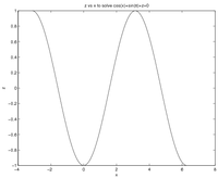
MyFun = @(xa, ya, za) cos(xa) + sin(ya) + za
xVals = linspace(-pi, 2*pi, 200);
yVal  = pi;
for k=1:length(xVals)
     [zVals(k), fVals(k)] = fzero(@(zDummy) MyFun(xVals(k), yVal, zDummy), 12);
end
Now, zVals contains the values of (z) that will make the function equal to zero for the corresponding values of (x) in the xVals matrix. The plot is shown at right. You can prove to yourself that this is correct by re-arranging the equation (f=0) to note that (z=-cos(x)-sin(y)) and, if (y=pi), (z=-cos(x)).
Two Parameters
The next logical expansion is to allow both (x) and (y) to change. There are two fundamentally different ways to approach this problem — either (x) and (y) can be represented by one-dimensional vectors and accessed as such or they can be created using a meshgrid structure. The latter will take up more memory, but at least all the matrices will be the same size and all entries can be accessed using the same row and column notation. As help for how you might set up such a problem, imagine that you want to find the roots of some function (f(alpha, beta, gamma)) — and you know (alpha) goes from 1 to 11 by 2 and (beta) goes from 10 to 100 by 10. Assuming you call the first variable Alpha and the second variable Beta, you can create a matrix Gamma with the code as follows:
[Alpha, Beta] = meshgrid(1:2:11, 10:10:100);
[Rows, Cols] = size(Alpha)
Gamma = zeros(Rows, Cols);
for R = 1:Rows
    for C = 1:Cols
        Gamma(R, C) = fzero(@(GammaDummy} f(Alpha(R, C), Beta(R, C), GammaDummy), <initial guess or bracket>)
    end
end
You could then visualize it with a mesh with contours using:
meshc(Alpha, Beta, Gamma)
Since fzero can only solve one value at a time, the double for loop is a useful way of sweeping through each possible set of parameters and storing the results in an organization structure that will lend itself to surface plotting later. The above is a demonstration of how a double loop might work. Note also that beta and gamma are built-in MATLAB functions — thus the use of capitals to avoid redefining built-in functions!
Questions
Post your questions by editing the discussion page of this article. Edit the page, then scroll to the bottom and add a question by putting in the characters *{{Q}}, followed by your question and finally your signature (with four tildes, i.e. ~~~~). Using the {{Q}} will automatically put the page in the category of pages with questions — other editors hoping to help out can then go to that category page to see where the questions are. See the page for Template:Q for details and examples.
External Links
References
![]()