I am attempting to install the package tidy verse in R studio and receiving these errors.
> install.packages('tidyverse')
also installing the dependency ‘rstudioapi’

  There is a binary version available but the source version is later:
           binary source needs_compilation
rstudioapi  0.9.0   0.10             FALSE

trying URL 'https://cran.rstudio.com/bin/macosx/el-capitan/contrib/3.5/tidyverse_1.2.1.tgz'
Content type 'application/x-gzip' length 88754 bytes (86 KB)
==================================================
downloaded 86 KB


The downloaded binary packages are in
    /var/folders/kn/b21xc36111z157czpz0swc900000gn/T//RtmpeVGvVh/downloaded_packages
installing the source package ‘rstudioapi’

trying URL 'https://cran.rstudio.com/src/contrib/rstudioapi_0.10.tar.gz'
Content type 'application/x-gzip' length 61888 bytes (60 KB)
==================================================
downloaded 60 KB

Error in loadNamespace(j <- i[[1L]], c(lib.loc, .libPaths()), versionCheck = vI[[j]]) :
  there is no package called ‘assertthat’
Calls: time.to ... tryCatch -> tryCatchList -> tryCatchOne -> <Anonymous>
Execution halted
Warning in install.packages :
  installation of package ‘rstudioapi’ had non-zero exit status

The downloaded source packages are in
    ‘/private/var/folders/kn/b21xc36111z157czpz0swc900000gn/T/RtmpeVGvVh/downloaded_packages’
In addition I’ve attempted to install in base R and receive the same message. I’ve gone to the temporary folders and unzipped the package and moved that over to the library folder. When I attempt library(assertthat) it gives me an error that there is not a valid package installed.
I’ve successfully installed tidyverse before on this machine, but when trying to use it this time it told me it was not installed, so I’ve attempted to reïnstall it.
Содержание
- library(tidyverse) fails on pre-1.1 versions of RStudio due to lack of getThemeInfo #83
- Comments
- Footer
- R-bloggers
- R news and tutorials contributed by hundreds of R bloggers
- Dataframes and the tidyverse
- Credibly Curious
- 2020-05-29
- Error in loadNamespace(Name) : There is No Package Called ‘here’
- Nicholas Tierney
- Install the package
- Why does that work?
- Another Error: Error in install.packages : object ‘here’ not found
- Another error: Warning in install.packages : package ‘emo’ is not available (for R version 3.6.2)
- Problem solving: Is the package perhaps misspelt?
- Problem solving: Does the package exist on CRAN?
- Why write this blog post?
- Thanks
library(tidyverse) fails on pre-1.1 versions of RStudio due to lack of getThemeInfo #83
When loading the tidyverse with library(tidyverse) in RStudio 1.0.153, the following error occurs:
Working backwards, the error occurs in text_col when it calls getThemeInfo . The function checks to ensure that rstudioapi is available, but not whether the version in use has getThemeInfo available. This can be isolated as:
Running the command on the same computer in the latest release of RStudio does not generate an error.
The text was updated successfully, but these errors were encountered:
I’m experiencing the same error using RStudio Server v.1.1.355
This fixed it for me:
@tiernanmartin I think that’s a different problem, but it’s also fix in the dev version
After:
install.packages(«tidyverse»)
tidyverse 1.1.1 1.2.1 FALSE
Warning in install.packages :
running command ‘»C:/PROGRA 1/R/R-32 1.4/bin/x64/R» CMD INSTALL -l «C:UsersUserDocumentsRwin-library3.2» C:UsersUserAppDataLocalTempRtmpGQjwZM/downloaded_packages/tidyverse_1.2.1.tar.gz’ had status 1
Warning in install.packages :
installation of package ‘tidyverse’ had non-zero exit status
library(tidyverse)
Error in library(tidyverse) : there is no package called ‘tidyverse’
. this problem is only on my home laptop (my work computer runs the same code fine).
What is going on?
hi, Rstudio Version 1.1.423
After installing R3.4.4 (2018-03-15) I have a similar problem, I get this:
library(tidyverse)
Error: package or namespace load failed for ‘tidyverse’ in loadNamespace(i, c(lib.loc, .libPaths()), versionCheck = vI[[i]]):
there is no package called ‘tidyr’»
Rstudio Version 1.1.423
© 2023 GitHub, Inc.
You can’t perform that action at this time.
You signed in with another tab or window. Reload to refresh your session. You signed out in another tab or window. Reload to refresh your session.
Источник
R-bloggers
R news and tutorials contributed by hundreds of R bloggers
Dataframes and the tidyverse
Posted on February 12, 2017 by geraldbelton in R bloggers | 0 Comments
The data frame is the primary structure for working with data in R. Whenever you have data that is arranged in a spreadsheet-like fashion, the default receptacle for that data in R is the data frame. In a data frame, each column contains measurements on one variable, and each row contains measurements on one case. All of the data in a column must be of the same type (numeric, character, or logical).
R has been around for more than 20 years now, and some things that worked well 20 years ago are less than ideal now. Consider how your mobile phone has changed over the last 20 years:
 Making changes to things as basic as data frames in R is difficult. If you change the definition of a data frame, then all of the existing R programs that use data frames would have to be re-written to use the new definition. To avoid this kind of problem, most development in R takes place in packages.
The R package “tibble” provides tools for working with an alternative version of the data frame. A tibble is a data frame, but some things have been changed to make using them a little bit easier. The tibble package is part of the tidyverse, a set of packages that provide a useful set of tools for data cleaning and analysis. The tidyverse is extensively documented in the book R For Data Science. In keeping with the open-source nature of R, that book is available free online: http://r4ds.had.co.nz/.
You can load tibble, along with the rest of the tidyverse tools, like this:
The first time you do this, you will probably get an error message.
In that case, you need to install tidyverse:
You only need to do this installation once, but when you start a new R session you will need to reload the package with the library() command.
Tibbles are one of the unifying features of the tidyverse, but most other R packages produce data frames. You can use the “as_tibble()” command to convert a data frame to a tibble:
There are some things that happen when you load a normal data frame that don’t happen when you load a tibble. On the plus side, tibble() doesn’t change the structure of your data. The data.frame() command will convert character strings to factors, unless you remember to tell it not to do that. Tibble won’t create row names. Tibble also won’t change the names of you variables.
This last feature can seem like a bug if you aren’t expecting it. One very common way to get data into R is to import it from a CSV file. CSV files are often created from Excel spreadsheets, and the column headings on Excel spreadsheets often don’t conform to the R standards for variable names. Since tibble doesn’t change variable names, you can end up with column names that are not proper R variable names. For example, they might include spaces or not start with a letter. To refer to these names, you’ll need to enclose them in backticks. For example:
`Feb Data` #contains space
Tibbles have a nice print method that, by default, shows only the first ten rows of data, and the number of columns that will fit on a screen. This keeps you from flooding your console with data.
You can control the number of rows and the width of the displayed data by explicitly calling ‘print.’ ‘width = Inf’ will print all of the columns.
You can look at the structure of an object, and get an overview of it, with the str() command:
Here are some more ways to look at basic information about a tibble (or a regular data frame):
Summary() provides a statistical overview of a data set:
To specify a single variable within a data frame or tibble, use the dollar sign $ . R has another way of doing this, using column numbers, but using the dollar sign will make it much easier to understand your code if someone else needs to use it, or if you come back to look at it months after writing it.
- Use data frames, and in particular, use the tidyverse and tibbles.
- Always understand the parameters of your data frame: the number of rows and columns.
- Understand what type of variables you have in your columns.
- Refer to your columns by name, using $ , to make your code more readable.
- When in doubt, use str() on an object.
Источник
Credibly Curious
Nick Tierney’s (mostly) rstats blog
2020-05-29
Error in loadNamespace(Name) : There is No Package Called ‘here’
Nicholas Tierney
This error (or a variant of it) is quite common when using R:
Another variant is:
Let’s list out some ways that you can address this issue.
Install the package
Install the package that is claimed not to be there. That is, for this error:
You install the PKG package (use your package name intead of PKG ):
Why does that work?
is given because R is looking for a package to use, and it cannot find that package. Installing your package means that R can find it, and load it so you can use it!
Another Error: Error in install.packages : object ‘here’ not found
This happens when you write:
You need to write the package that you want to install in quotes:
Why? Well R thinks here is an object, but it requires the R package to be in quotes.
Now, that might not feel like the best reason — the truth is it is to do with a thing called Non Standard Evaluation (NSE), but going into more detail than that is beyond the scope of this blog post.
What I would suggest is this, internalise:
When installing R packages, put the package in quotes: “package”
Another error: Warning in install.packages : package ‘emo’ is not available (for R version 3.6.2)
This can happen if you write:
Why? Well, it could be one of the following below errors:
- Package name misspelt
- Package might not exist on CRAN
It is quite likely that it is not to do with your version of R.
Problem solving: Is the package perhaps misspelt?
I have, more often than I care to admit, had a spelling mistake that caused me to go on a rabbit hole.
Problem solving: Does the package exist on CRAN?
Type “PKG CRAN rstats” into a search engine
Perhaps you might find the right spelling, in which case, install the package with the right spelling using install.packages .
Perhaps you might find that it is on github (or bitbucket or gitlab), not on CRAN.
Let’s take a github example. You need to install an R package from github with a different command.
Let’s say we want to install the “treezy” package from github. You scroll down and find the instructions here:
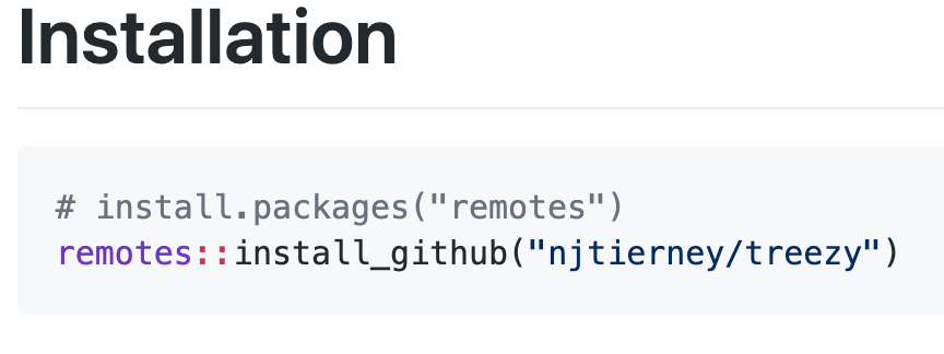
So you will need to do two things:
- Install remotes from CRAN ( install.packages(«remotes» )
- Run remotes::install_github()
Similarly there are packages for R packages that you might find on other repositories such as gitlab ( install_gitlab ) or bitbucket ( install_bitbucket ).
Why write this blog post?
I teach an introduction to data analysis class, and many students encounter this error:
but they do not have the skills and experience to identify how to solve this problem. In class, I decided to showcase how I would try to solve this problem, live, on zoom, to my class. So I googled the error, and then I discovered that the top hit isthis stack overflow page, which was decidedly not helpful for the problem that my students had.
So I wrote this blogpost.
Hopefully it’s helpful!
Next up in this series is tackling this problem:
Thanks
Thanks to Emi Tanaka and Miles McBain for their suggestions on a few helpful additions to the blog post!
Источник
Credibly Curious
Nick Tierney’s (mostly) rstats blog
2020-05-29
Error in loadNamespace(Name) : There is No Package Called ‘here’
Nicholas Tierney
This error (or a variant of it) is quite common when using R:
Another variant is:
Let’s list out some ways that you can address this issue.
Install the package
Install the package that is claimed not to be there. That is, for this error:
You install the PKG package (use your package name intead of PKG ):
Why does that work?
is given because R is looking for a package to use, and it cannot find that package. Installing your package means that R can find it, and load it so you can use it!
Another Error: Error in install.packages : object ‘here’ not found
This happens when you write:
You need to write the package that you want to install in quotes:
Why? Well R thinks here is an object, but it requires the R package to be in quotes.
Now, that might not feel like the best reason — the truth is it is to do with a thing called Non Standard Evaluation (NSE), but going into more detail than that is beyond the scope of this blog post.
What I would suggest is this, internalise:
When installing R packages, put the package in quotes: “package”
Another error: Warning in install.packages : package ‘emo’ is not available (for R version 3.6.2)
This can happen if you write:
Why? Well, it could be one of the following below errors:
- Package name misspelt
- Package might not exist on CRAN
It is quite likely that it is not to do with your version of R.
Problem solving: Is the package perhaps misspelt?
I have, more often than I care to admit, had a spelling mistake that caused me to go on a rabbit hole.
Problem solving: Does the package exist on CRAN?
Type “PKG CRAN rstats” into a search engine
Perhaps you might find the right spelling, in which case, install the package with the right spelling using install.packages .
Perhaps you might find that it is on github (or bitbucket or gitlab), not on CRAN.
Let’s take a github example. You need to install an R package from github with a different command.
Let’s say we want to install the “treezy” package from github. You scroll down and find the instructions here:
So you will need to do two things:
- Install remotes from CRAN ( install.packages(«remotes» )
- Run remotes::install_github()
Similarly there are packages for R packages that you might find on other repositories such as gitlab ( install_gitlab ) or bitbucket ( install_bitbucket ).
Why write this blog post?
I teach an introduction to data analysis class, and many students encounter this error:
but they do not have the skills and experience to identify how to solve this problem. In class, I decided to showcase how I would try to solve this problem, live, on zoom, to my class. So I googled the error, and then I discovered that the top hit isthis stack overflow page, which was decidedly not helpful for the problem that my students had.
So I wrote this blogpost.
Hopefully it’s helpful!
Next up in this series is tackling this problem:
Thanks
Thanks to Emi Tanaka and Miles McBain for their suggestions on a few helpful additions to the blog post!
Источник
downloading and running tidyverse package in R

Hi,
I’m trying to download the package ‘tidyverse’ in R studio for rna seq analysis. This will allow me to transfer Kallisto results into R.
I have used the following command: install.packages("tidyverse"). However, I get the following error message when I try to run the function library(tidyverse): Error in library(tidyverse) : there is no package called ‘tidyverse’.
I also tried the install packages option in r studio.
If anyone knows how to install this package please let me know.
Thankyou
seq
analysis
tidyverse
rna
• 2.3k views
Login before adding your answer.
Traffic: 2406 users visited in the last hour
[This article was first published on R – Gerald Belton, and kindly contributed to R-bloggers]. (You can report issue about the content on this page here)
Want to share your content on R-bloggers? click here if you have a blog, or here if you don’t.
The data frame is the primary structure for working with data in R. Whenever you have data that is arranged in a spreadsheet-like fashion, the default receptacle for that data in R is the data frame. In a data frame, each column contains measurements on one variable, and each row contains measurements on one case. All of the data in a column must be of the same type (numeric, character, or logical).
R has been around for more than 20 years now, and some things that worked well 20 years ago are less than ideal now. Consider how your mobile phone has changed over the last 20 years:
 Making changes to things as basic as data frames in R is difficult. If you change the definition of a data frame, then all of the existing R programs that use data frames would have to be re-written to use the new definition. To avoid this kind of problem, most development in R takes place in packages.
The R package “tibble” provides tools for working with an alternative version of the data frame. A tibble is a data frame, but some things have been changed to make using them a little bit easier. The tibble package is part of the tidyverse, a set of packages that provide a useful set of tools for data cleaning and analysis. The tidyverse is extensively documented in the book R For Data Science. In keeping with the open-source nature of R, that book is available free online: http://r4ds.had.co.nz/.
You can load tibble, along with the rest of the tidyverse tools, like this:
library(tidyverse)
The first time you do this, you will probably get an error message.
> library(tidyverse)
Error in library(tidyverse) : there is no package called ‘tidyverse’
In that case, you need to install tidyverse:
install.packages('tidyverse')
You only need to do this installation once, but when you start a new R session you will need to reload the package with the library() command.
Tibbles are one of the unifying features of the tidyverse, but most other R packages produce data frames. You can use the “as_tibble()” command to convert a data frame to a tibble:
as_tibble(iris)
#> # A tibble: 150 × 5
#> Sepal.Length Sepal.Width Petal.Length Petal.Width Species
#> <dbl> <dbl> <dbl> <dbl> <fctr>
#> 1 5.1 3.5 1.4 0.2 setosa
#> 2 4.9 3.0 1.4 0.2 setosa
#> 3 4.7 3.2 1.3 0.2 setosa
#> 4 4.6 3.1 1.5 0.2 setosa
#> 5 5.0 3.6 1.4 0.2 setosa
#> 6 5.4 3.9 1.7 0.4 setosa
#> # ... with 144 more rows
There are some things that happen when you load a normal data frame that don’t happen when you load a tibble. On the plus side, tibble() doesn’t change the structure of your data. The data.frame() command will convert character strings to factors, unless you remember to tell it not to do that. Tibble won’t create row names. Tibble also won’t change the names of you variables.
This last feature can seem like a bug if you aren’t expecting it. One very common way to get data into R is to import it from a CSV file. CSV files are often created from Excel spreadsheets, and the column headings on Excel spreadsheets often don’t conform to the R standards for variable names. Since tibble doesn’t change variable names, you can end up with column names that are not proper R variable names. For example, they might include spaces or not start with a letter. To refer to these names, you’ll need to enclose them in backticks. For example:
`Feb Data` #contains space
Tibbles have a nice print method that, by default, shows only the first ten rows of data, and the number of columns that will fit on a screen. This keeps you from flooding your console with data.
> irises <- as_tibble(iris)
> irises
# A tibble: 150 × 5
 Sepal.Length Sepal.Width Petal.Length Petal.Width Species
 <dbl> <dbl> <dbl> <dbl> <fctr>
1 5.1 3.5 1.4 0.2 setosa
2 4.9 3.0 1.4 0.2 setosa
3 4.7 3.2 1.3 0.2 setosa
4 4.6 3.1 1.5 0.2 setosa
5 5.0 3.6 1.4 0.2 setosa
6 5.4 3.9 1.7 0.4 setosa
7 4.6 3.4 1.4 0.3 setosa
8 5.0 3.4 1.5 0.2 setosa
9 4.4 2.9 1.4 0.2 setosa
10 4.9 3.1 1.5 0.1 setosa
# ... with 140 more rows
You can control the number of rows and the width of the displayed data by explicitly calling ‘print.’ ‘width = Inf’ will print all of the columns.
irises %>%
 print(n=5, width = Inf)
You can look at the structure of an object, and get an overview of it, with the str() command:
> str(irises)
Classes ‘tbl_df’, ‘tbl’ and 'data.frame': 150 obs. of 5 variables:
 $ Sepal.Length: num 5.1 4.9 4.7 4.6 5 5.4 4.6 5 4.4 4.9 ...
 $ Sepal.Width : num 3.5 3 3.2 3.1 3.6 3.9 3.4 3.4 2.9 3.1 ...
 $ Petal.Length: num 1.4 1.4 1.3 1.5 1.4 1.7 1.4 1.5 1.4 1.5 ...
 $ Petal.Width : num 0.2 0.2 0.2 0.2 0.2 0.4 0.3 0.2 0.2 0.1 ...
 $ Species : Factor w/ 3 levels "setosa","versicolor",..: 1 1 1 1 1 1 1 1 1 1 ...
Here are some more ways to look at basic information about a tibble (or a regular data frame):
> names(irises)
[1] "Sepal.Length" "Sepal.Width" "Petal.Length"
[4] "Petal.Width" "Species"
> ncol(irises)
[1] 5
> length(irises)
[1] 5
> dim(irises)
[1] 150 5
> nrow(irises)
[1] 150
Summary() provides a statistical overview of a data set:
> summary(irises)
 Sepal.Length Sepal.Width Petal.Length
 Min. :4.300 Min. :2.000 Min. :1.000
 1st Qu.:5.100 1st Qu.:2.800 1st Qu.:1.600
 Median :5.800 Median :3.000 Median :4.350
 Mean :5.843 Mean :3.057 Mean :3.758
 3rd Qu.:6.400 3rd Qu.:3.300 3rd Qu.:5.100
 Max. :7.900 Max. :4.400 Max. :6.900
 Petal.Width Species
 Min. :0.100 setosa :50
 1st Qu.:0.300 versicolor:50
 Median :1.300 virginica :50
 Mean :1.199
 3rd Qu.:1.800
 Max. :2.500
To specify a single variable within a data frame or tibble, use the dollar sign $. R has another way of doing this, using column numbers, but using the dollar sign will make it much easier to understand your code if someone else needs to use it, or if you come back to look at it months after writing it.
> head(irises$Sepal.Length)
[1] 5.1 4.9 4.7 4.6 5.0 5.4
> summary(irises$Sepal.Length)
 Min. 1st Qu. Median Mean 3rd Qu. Max.
 4.300 5.100 5.800 5.843 6.400 7.900
To recap:
- Use data frames, and in particular, use the tidyverse and tibbles.
- Always understand the parameters of your data frame: the number of rows and columns.
- Understand what type of variables you have in your columns.
- Refer to your columns by name, using
$, to make your code more readable. - When in doubt, use
str()on an object.
In this very first lesson, you’ll learn how to:
- get R up and running on your computer.
- interact with R by typing statements into the console and seeing the results of those statements.
- define your own objects and use those objects in subsequent statements.
- create a new script and run some statements from that script.
- get help with R.
- install and load libraries.
Download R and RStudio
To begin using R, you’ll need to download two pieces of software:
- Head to cloud.r-project.org to download and install the version of R appropriate for your computer, whether Windows, Mac, or Linux. Note that if you have a newer MacBook with an Apple M1 chip, make sure to install the appropriate version of R (labeled
Apple silicon arm64on the download page), and not the version designed for older Intel-based MacBooks.1 - Head to www.rstudio.com and download RStudio. If prompted to choose your version, you’ll want “RStudio Desktop,” which is free and, like R, available for Windows, Mac, and Linux.
Why two programs? Well, R is the program that does most of the raw computational work, while RStudio is a graphical front end for R (called an “integrated development environment,” or IDE) that offers a lot of creature comforts. You’ll work entirely within RStudio; meanwhile, RStudio will interface with R behind the scenes, without your ever needing to open the R program itself. Loosely speaking, if you imagine that analyzing data is like driving a car, then RStudio is the steering wheel and the pedals, while R is the engine.2 That’s why you need to install R in order for RStudio to work: if you try to drive a car without an engine, you’re not going to get very far.
First steps
Go ahead and open up RStudio for the first time. On a Mac or Windows machine, this is as simple as finding where you’ve installed the RStudio app (not the R app) and double-clicking its icon. You should see something like this (with possible minor aesthetic differences, depending on your computer’s operating system):
There’s a lot here, and it might seem overwhelming at first. Here’s a brief summary of what you’re looking at:
- The left panel, with the blinking cursor and the
>symbol, is the console. This is where R statements get evaluated and where the results of those statements get printed. - The top right panel shows your workspace. In these lessons, you’ll mainly use this panel to import data sets. But this panel allows you to do some other handy things, too, like examine a history of prior statements that you’ve asked R to evaluate in the console.
- Finally, the bottom-right panel is mainly used for plots, packages, and help. We’ll see this in action soon.
Interacting with R
For now, just focus on the left-hand panel (the console). More specifically, focus on the blinking cursor in the console, right next to the angle bracket (>). That > symbol is a prompt; it’s R’s way of saying, “Tell me what to do by typing statements right here.” Below I’ve circled it in red:
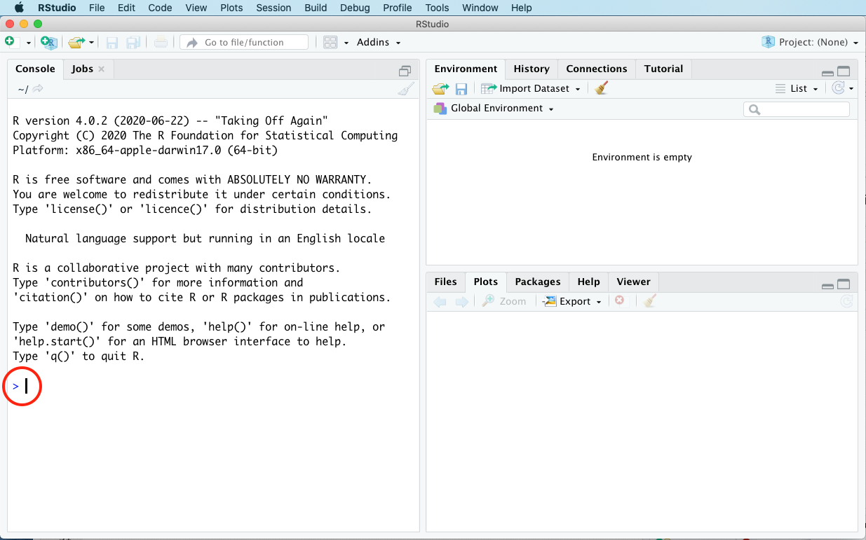
Where see you that prompt (>), type the following statement:
2+3Then hit Enter to run the statement. R should print out 5 right underneath where you typed 2+3, and then it should give you a new prompt (> + blinking cursor) immediately below that. In other words, your screen should now look like this:
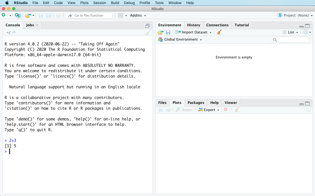
Congratulations! You’ve just run your first line of R code — in this case, a statement that tells R to do some simple arithmetic. In the console, R is telling you that the result of evaluating the statement 2+3 is 5.
You might be confused by the little [1] in front of the 5. That’s R’s way of telling you that it has only 1 number to report, and that this number is 5. This habit of R’s might initially seem like oversharing, but it will make a lot more sense later, when we start doing calculations that produce multiple numbers as outputs and we might want some handy way of referencing, say, the 104th number.
This example, while simple, illustrates the basic idea of interacting with R:
- You write statements (also known as commands or lines of code), and run those statements in the console.
- R evaluates those statements and does something—for example, printing out the result of a calculation or making a plot.
Some statements, like 2 + 3, are simple. Other statements, like log10(1000) + 4^2 - 15.85841, are a bit more complex. (Try that one in the console.)3 Soon, you’ll start to chain multiple statements together to form a program. But in the very beginning, learning R mostly means learning which statements do which things!
How you’ll get feedback
Every lesson in this book depends on getting immediate feedback: I’ll show you what R statements you need to write in order to accomplish a given task, together with what you should expect to see as a result of executing those statements. In my experience, this is the best way learn R (or any programming language).
Above, I provided this feedback via screen shot. This worked OK. But screen shots aren’t really the best way to give you the feedback you need. Not only are they tedious for me, but they’re also inefficient for you: they show a bunch of extraneous information, with the relevant feedback buried in a corner somewhere, perhaps with a silly red circle drawn around it.
So from here on, we’ll adopt the following convention. Whenever you’re supposed to evaluate a statement (like 2+3) and to compare your result with mine, you’ll see it written in two boxes, like this:
## [1] 5The first box shows what you’re supposed to type. Immediately below that, the second box shows what the result should be, whether it’s something printed to console (like we see here) or a plot (like you’ll see below). Note that you won’t actually see the little ## symbols printed in your console. Those ## symbols are there so that you can distinguish intended input (first box, no ##) from expected output (second box, with ##) at a quick glance.
Let’s see one more explicit example of this convention in action. We’ll add 1 and 4, and then multiply the result by 3:
## [1] 15The two blocks above are telling you: 1) that you should type in 3*(1+4) and then hit Enter (first block); and 2) that you should see [1] 15 printed out to the console as a result (second block). Again, the [1] 15 means that R has 1 number to report as a result of what you asked it to do, and that this number is 15.
I’ll mostly stick with this convention for providing feedback, saving screen shots only for when they’re necessary.
R as a calculator
You probably got the sense from the examples above you can treat R as a simple calculator. Indeed, R works exactly as you’d expect it to in this regard: it obeys the standard order of operations that you learned in grade school, and it also knows all the important “fancy” functions like logarithms and cosines and exponentials that you learned in high school. Here we’ll calculate the base-10 logarithm of 1000:
## [1] 3You can also treat R like a graphing calculator, using the curve function. Try, for example, typing in the following statement:
curve(x^2 - 3*x + 1, from=0, to=5)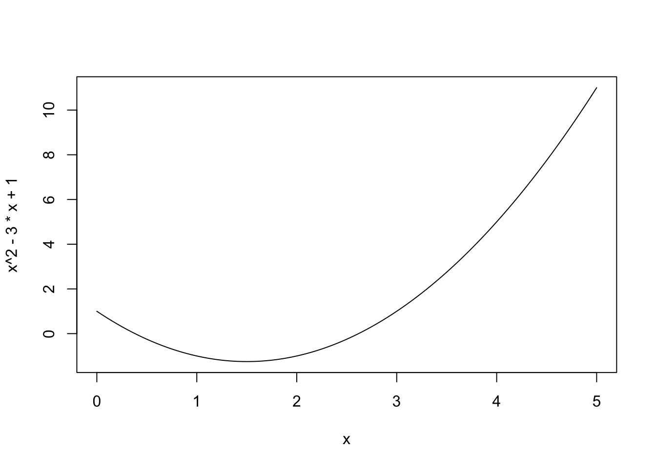
This statement plots the curve (f(x) = x^2 — 3x + 1) over the domain (0 leq x leq 5). The three inputs to curve are called arguments:
x^2 - 3*x + 1is the curve you want to plot.from=0andto=5says that you want to start the curve at (x=0) and end it at (x=5).
When you evaluate the statement by hitting Enter, nothing gets printed to the console, but you should see a graph pop up automatically in the Plots tab, in the lower-right panel on your screen. (Displaying plots is one of the main uses of that lower-right panel, although we’ll cover a couple of other uses later.)
If you want to get some practice, try any of the following examples, or else just make up your own.
30/10
5^2
sqrt(9)
log(7.4)
exp(2)
curve(cos(x), from=0, to=4*pi)
Note that to R:
- the four basic arithmetic operations are
+,-,*, and/. logmeans natural log, whilelog10means the base-10 log.x^ameans “raise x to the power a.”- But if you want to raise the mathematical constant (e = 2.718…) to some power (a), use
exp(a). - For trigonometric functions (like
cos,sin,tan, etc.), angles are assumed to be in radians.
R is case sensitive
Statements in R are case-sensitive. If you use upper case where lower case is expected, or vice versa, you’ll get an error. So if, for example, you typed Curve rather than curve, you’d get an error telling you that there is no such thing as a function called Curve:
Curve(x^2 - 3*x + 1, from=0, to=5)## Error in Curve(x^2 - 3 * x + 1, from = 0, to = 5): could not find function "Curve"Be aware of this case-sensitivity. It’s a common source of coding errors for beginners.
Objects
We’ve seen that using R as a (graphing) calculator is pretty straightforward. But to do anything more interesting than basic arithmetic, we need to learn how to assign values to objects.4
In computer programming, an object is analogous to an envelope or a file folder. It’s a place where information can be stored, given a label, and accessed later. Creating objects helps us break complex tasks down into a series of simpler tasks.
Let’s create your first object. Run the following statement in the console:
Nothing gets printed to the console when you run this statement. But under the hood, R has created an object called foo and stored the value 3 in that object.
Let’s unpack the statement foo = 3 piece by piece. All assignment statements in R have the same basic structure:
3is the value of the object. In our file-folder analogy, this is like the contents of the folder.foois the name of the object. In our file-folder analogy, this is like the label on the folder. Here we called the objectfoo, but you can call objects in R pretty much anything you want, with a handful of exceptions.=is called the “assignment operator.” It tells R to assign the value on the right (3) to the object on the left (foo).
If we now ask R what foo is, it will tell us:
## [1] 3The reason we assign values to objects is so that we can use those objects in subsequent calculations. It’s like a souped-up version of the “memory” function on your calculator. To illustrate this, let’s create an object called bar that stores the results of the computation (4 + log_{10}(100)). Since (log_{10}(100) = 2), this calculation should give us 6.
Again, nothing gets printed to the console when we create an object and assign it a value. But, remember, once we’ve created the object, we can type its name into the console, and R will tell us what value is stored there:
## [1] 6More importantly, now we can use this object in a subsequent computation, just like we’d use any number:
## [1] 10Creating objects—that is, storing intermediate results in user-defined objects, and re-using those results in subsequent calculations—may not seem like a big deal now. After all, we’re just messing around with basic arithmetic. But as you’ll soon learn, the ability to create your own objects is a source of great power. That’s because it allows us to write a complex data analysis as a sequence of many smaller, simpler steps. And that’s the way we accomplish pretty much anything complex in life, whether it’s running a data analysis, auditing a bank, or building a house:
- break the complex task down into simpler tasks.
- accomplish each task in isolation, using the products of earlier tasks to help us with the next task.
- stitch the tasks together in the proper order to accomplish the overall goal.
We could summarize this “basic mantra of data science” as follows.
The basic mantra of data science: manage complexity by breaking complex tasks down into simple tasks, and then stitching the simple tasks together.
In the next section, we’ll learn how scripts can make this process a lot more manageable.
Scripts
In our previous examples, you learned to interact with R by typing statements like 2+3 or sqrt(9) directly into the console, where you see the > prompt. This works OK for simple statements, but it’s actually not the best way to interact with R—especially when we start chaining together complex statements to analyze data.
Instead, you should learn to work with scripts. A script is a file that collects multiple statements (i.e. lines of R code) in a single document, which always ends in a .R suffix.
Your basic workflow in RStudio should look like this.
- Create a script with the goal of solving some specific tasks.
- Write statements in your script, saving them for subsequent modification or re-use.
- Run those statements in the console to produce the desired output or behavior.
- View the results, usually either in the console or the
Plotstab of RStudio’s lower-right panel.
There are many advantages to working with scripts, which we’ll discuss below. For now let’s focus on the “how” and “what” rather than the “why.”
Creating and running scripts
To create a new R script, go to the File Menu and choose New File > R Script. Your screen should now look something like this:

Before there were three panels; now there are four. The bottom left panel is your old friend, the console. But now there’s a (new) top left panel called the code editor. RStudio’s code editor allows you to create, open, and edit R scripts. When you opened the File menu and chose New File > R script, you conjured into existence a new, blank script whose default name is probably something like Untitled1.R. In the lessons to follow, this panel is where you’ll do most of your actual work, by creating and editing scripts (.R files) that encode the steps in a data analysis.
Go ahead and type the following two statements in the new script you just created. Do not type them directly in the console. Put each statement on its own line in your script, and then save the script, giving it whatever name you want (e.g. my_first_script.R):
foo = 1 + 2
foo + 7
These statements: 1) create an object called foo that is assigned a specific value (i.e. 3, the result of 1 + 2); and then 2) add 7 to foo. We should get 10 as a result, right? But when you type these statements in your script, nothing actually happens. That’s because you need to run these statements in the console in order to get R to evaluate them.
The easiest way to run statements from your script is to highlight those statements with your mouse, and then use the keyboard shortcut Control-Enter (Command-Enter works too if you’re on a Mac). When you do this, you should see the statements themselves, followed by their result, appear in your console, like this:
## [1] 10And that’s it—your first R script. From here on, when I give you R commands to run, you should first write them in a script, and then run them in the console. It might feel clunky at first, but you should practice this way of doing things, because it will indispensable when things get more complex.
Two further notes on running statements from a script:
- If you just want to run a single line from your script, you don’t have to highlight it. You can just click anywhere on that line and then hit
Control-Enter. - You can also run statements (either individually or as a block) using the
Runbutton at the top of the code editor. I personally find this less user-friendly, but your mileage may vary.
A slightly more interesting script
OK, so that first script was a bit simple. Below, I’ve given you one that’s slightly more interesting. You can safely include the little notes after the # symbol, which are called “comments.” R ignores anything in a script the right of the # symbol, allowing you to write little explanations (for yourself or others) about what your code is doing.
# Load one of R's built-in data sets about cars
data(mtcars)

# Fit a straight line for mpg vs hp and plot the result.
mpg_model = lm(mpg ~ hp, data=mtcars)
plot(mtcars$hp, mtcars$mpg)
abline(mpg_model)
coef(mpg_model)
Create a new blank script, and then type5 this entire chunk of R code, word for word, into your script. Don’t worry too much about the details of the individual statements; we’ll cover those in later lessons.
Now highlight everything in the script, and hit Control-Enter to run it. You should see the plot below:
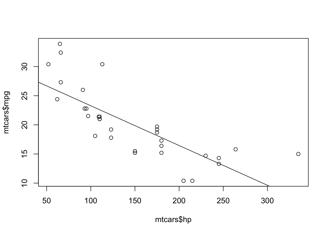
And you should also see the following information printed in your console:
## (Intercept)          hp
## 30.09886054 -0.06822828
Each dot in the plot represents a car. The x coordinate of the dot represents the horsepower (hp) of that car’s engine. The y coordinate represents that car’s gas mileage (mpg). The line you see is the result of fitting a linear regression model to estimate the systematic relationship between mileage and horsepower. The two numbers printed in your console tell you the (y)-intercept and slope of the trend line. Unsurprisingly, cars with more powerful engines tend to get lower gas mileage (hence the negative slope).
This code chunk exhibits two important ideas we’ve covered: 1) the use of = to assign values to objects; and 2) the re-use of those objects in subsequent statements. For example, the statement mpg_model = lm(mpg ~ hp, data=mtcars) fits a straight line to mpg versus hp, storing the result in an object that I called mpg_model. This mpg_model object is then re-used in two subsequent statements, abline(mpg_model) and coef(mpg_model), which draw the line through the point cloud and print the intercept/slope to the console, respectively.
So there you have it: you’ve run and visualized your first data analysis in R! I hope you’re beginning to get a feel for the basic RStudio workflow. You create a script organized around some specific task. Then you:
- write statements in your script, saving them for subsequent modification or re-use.
- run those statements in the console to produce the desired output or behavior.
- view the results, usually either in the console or the
Plotspanel
In more complex data analyses, you will typically iterate these three steps, gradually building up complexity until you’ve accomplished what you set out to do.
Organizing your data analyses around scripts is probably the single most important “best practice” of using R. It’s perfectly fine to type statements directly into the console every now and again, especially if you’re in more of an “exploratory” mode. But if you find yourself doing this repeatedly, especially with complex statements that build on previous statements, you should probably stop and ask yourself: “Would I be better off writing these statements in a script instead, so that I can save, re-use, and modify them later?” Usually the answer is yes!
Why can’t I just point and click?
This way of interacting with R—writing statements in a script and then running those statements in the console—is called a “command-line interface” or a “REPL” (pronounced “reeple,” for Read-Evaluate-Print Loop). It may seem unfamiliar or even intimidating at first. It’s certainly different from popular programs you might be used to, where you do a lot of pointing and clicking. To R beginners, the command-line interface can even feel like a step backward in time—sort of like you’re interacting with a “dumb” computer from the 1970s rather than something “smart” from the 21st century, with a mouse or a touch screen.
“Why do I have to type literally everything?” you might wonder. “Why can’t I click on menus and buttons that do this stuff for me?”
I understand this reaction. But let me try to convince you that the command-line interface is actually a huge advantage for doing data science! It’s true that the learning curve is steeper than with more familiar “point and click” software packages. But with R, the results of running a complex analysis don’t require that you remember a long, detailed succession of clicks and menu options. Instead, those results rely upon a series of written commands that do exactly what they say. So, for example, if you want to re-run your analysis on a new data set—perhaps because you collected some more data—you don’t need have to remember which buttons you clicked or which menu options you chose in order to get your new results. You just have to load the new data set and re-run your script from beginning to end—possibly tweaking it here and there, as required.
Here are five other advantages to this way of interacting with R, via scripts and the console:
- Scripts make it simple to save your work and pick up where you left off, without having to remember what you’ve accomplished already.
- Scripts make it easy to modify a complex analysis by adding or changing steps in the middle of a long chain of statements. (No
Control-Zrequired!) - Scripts make your analysis shareable: just save the .R file and post it to a site like GitHub.
- Scripts make your analysis reproducible, since anyone—including a future version of yourself—can read the script and see/repeat exactly what you’ve done.
- Scripts make it much easier to diagnose and correct errors in your analysis, because—unlike, say, in other widely used data-analysis programs—an error always arises from some specific statement that’s written down in black and white for anyone to see.6
As I hope you’ll come to appreciate over the lessons to come, these advantages far outweigh the familiar comforts of mice and menus.
Getting help
Everyone needs help with R at some point or another. In fact, the more you use R, the more you’ll find yourself relying on various help resources. In my life as a teacher and researcher, I look for R help all the time, and you will, too.
Here are your best bets.
-
Search the web. There’s a huge and very active community of R users out there, and many of them like to post about their R problems, or their solutions to other people’s R problems, online. If in doubt, just Google your question, e.g. “How do I find the maximum of two numbers in R?” Chances are very, very good that your question has been asked and answered before.
-
Search R’s own help files. For example, suppose you wanted to figure out how to calculate the median of a bunch of numbers in R. You could go to the
Helptab in the lower-right panel, and typemedianinto the search bar. You’d see several options pop up, one of which is the function calledmedian. Click on it, and the help page for that function will be displayed. It will show you how to use the function, and even give you examples at the bottom of the help page. -
If you want help on a specific function—say, for example, the function
log10—you can type a question mark, followed by the function’s name, into the console. Try, for example, running this statement:
Personally, I use option 1 about 70% of the time, option 3 about 30% of the time, and option 2 about 0% of the time (since all of R’s help files are on the web anyway, and will come up in a web search if they’re useful).
My advice
Now that we’ve covered the basics of R scripts and getting help, here’s my advice for how best to use this book to learn R.
- Type out my commands into your own script. Don’t just copy/paste. Copying and pasting is lazy, and you’ll never build muscle memory that way, any more than you can learn to ride a bike by watching someone else ride a bike.
- Execute the commands and compare your results to mine. (Remember our convention on How you’ll get feedback from above.)
- Be an active learner. Once you start to learn a bit of R, try executing variations on the commands I’ve given to see what you get. Trying articulating out loud in your own words what each command is doing and why it produces the behavior it does. This is a great way to build familiarity with the R environment.
Invariably, I have students in my large data science classes at UT who think they understand R on the basis of these lessons, but then do poorly on quizzes and tests. When I talk with them about their study habits, more often than thought it turns out that they’ve been plowing through these walk-throughs, blindly copying/pasting commands and hitting command enter at high speed, without dwelling on why the commands do what they do, and without absorbing the underlying ideas.
You cannot expect to just “copy/paste/command-enter” your way through these walk-throughs and come away with an understanding of R or data science. What’s true of learning R is true of learning pretty much anything: becoming an independent learner means actively engaging in the material.
Libraries
R has an enormous ecosystem of libraries, ranging from the simple to the very sophisticated. A library is a piece of software that provides additional functionality to R, beyond what’s contained in the basic R installation. If R is like a smart phone, then a library is like an app for the phone. And just like a phone app, a library is something you need to install only once, but load each time you want to use it.
Installing a library
Here we’ll install two libraries that we’ll use a lot in the lessons to follow: tidyverse and mosaic.
The first minute of this video gives a walk-through of how to install a library. (It’s with an older version of RStudio, though the process is still the same). But we’ll explain the steps here, too. Conveniently, libraries, also called “packages,” are installed from within RStudio itself.
Here are the steps to install tidyverse. The same process works for any library:
- In the lower right panel of RStudio, you’ll see a tab called
Packages. Click on it. - Under the
Packagestab, you’ll see a button at the top left of the panel calledInstall. Click on it. - In the window that pops up, type in the name of the package you want to install:
tidyverse. After a few letters, RStudio will start to auto-suggest options for you. Just keep typing until you seetidyverseas the only option. Then either click on it or hitTabto auto-complete the full name of the library. - Click the
Installbutton.
In response, R should print out a very long and seemingly ponderous “progress report” into the console. This “progress report” provides all kinds of interesting detail for R super-users, but it isn’t all that helpful if you’re a beginner—and because there’s just so much darn red text, it can even seem intimidating! But not to worry. R is just telling you, in its own long-winded way, that it’s downloading and installing a bunch of tidyverse-related files behind the scenes.7 Eventually it should stop with some kind of DONE message in the console and give you another prompt (>), at which point the library is installed and ready to be used.
Then repeat the whole process to install mosaic. If you got an error, see Dealing with installation errors, below.
Loading a library
Let’s practice loading the tidyverse library, which we’ll lean on heavily in most of these lessons. In R, you load a library using the library command, like this:
## ── Attaching packages ──────────────────────────────────────────────────────────────────────────────────────────────────── tidyverse 1.3.1 ──## ✓ ggplot2 3.3.5 ✓ purrr 0.3.4
## ✓ tibble 3.1.3 ✓ dplyr 1.0.7
## ✓ tidyr 1.1.3 ✓ stringr 1.4.0
## ✓ readr 2.0.1 ✓ forcats 0.5.1## ── Conflicts ─────────────────────────────────────────────────────────────────────────────────────────────────────── tidyverse_conflicts() ──
## x dplyr::filter() masks stats::filter()
## x dplyr::lag() masks stats::lag()If you see a similar set of messages to what’s shown above (possibly with some more rows called “Conflicts”), you’re good to go! Feel free to move on to the next lesson.
But if you haven’t installed the tidyverse library, executing this command will give you an error like this:
Error in library(tidyverse) : there is no package called ‘tidyverse’To avoid the error, you’ll first need to install tidyverse like we covered above.
Dealing with installation errors
R might issue a warning or tell you that it had a conflict when you installed these libraries. Despite sounding scary, these notices are almost certainly innocuous and can be safely ignored.
On the other hand, if R tells you that it had an error when installing, you’ll need to address that error before you move on. Luckily, most library installation errors are a result of having an old version of R, and therefore fixable with two simple steps:
- Install the latest version of R, from cloud.r-project.org.
- Install the latest version of RStudio, from www.rstudio.com.
Usually, it’s that simple.
If that doesn’t fix the problem, however, your next step is to try Googling the error message. (If you’re taking my class and show me the installation error message, that is precisely what I will do, unless it happens to be some particular error I’ve seen before.) Installation errors like this are rare, but they can happen, and they’re almost always due to some quirk of your particular computer (and therefore difficult to generalize about). The good news is whatever error you’re experiencing is almost surely not unprecedented in the history of R. In fact, the chances are good that someone, somewhere, has figured out what the error means and how to fix it.
In my large classes at UT-Austin, the most common (but still quite rare) library installation error I’ve seen tends to occur on Windows machines, and it looks something like the following:
The downloaded source packages are in
?/tmp/Rtmph4YKLX/downloaded_packages?
Updating HTML index of packages in '.Library'
Warning in install.packages :
cannot create file
'/opt/POC/lib64/Revo-7.3/R-3.1.1/lib64/R/doc/html/packages.html', reason
'Permission denied'
Yikes! Basically, what’s happening here is that you don’t have permission to write files to the directory where R wants to write files. (Hence 'Permission denied'!) This can happen if your computer is actually owned by someone else, e.g. your employer, but I’ve also seen it happen out of the blue to students who own their computers fair and square.
Fixing the error depends on which version of Windows you have, and so your best bet is to Google something like “Give permissions to files and folders in Windows” and follow whatever steps suggested by the collective wisdom of humanity.