Not sure if this is a new issue or not. I am getting this error and don’t quite understand the fix that was applied for #461 as this appears to be related to the fix.
Here is my call to train. The data set contains no NA:
fitWithXGBLinear <- train(target~.,
                                data=train,
                                method = 'xgbLinear',
                                tunrLength=3,
                                trControl = ctrl ,
                                metric="logLoss"
)
This produces the error:
Error in na.fail.default(list(target = c(10L, 8L, 8L, 12L, 1L, 1L, 4L,  :
  missing values in object
As shown below, my data set contains no NA. This data set is from a current kaggle competition:
> lapply(train, function(x) any(is.na(x)))
$a
[1] FALSE

$target
[1] FALSE

$b
[1] FALSE

$c
[1] FALSE
This data set is from a current kaggle competition:
'data.frame':   51336 obs. of  4 variables:
 $ a     :Class 'integer64'  num [1:51336] 1.06e+05 -9.81e+71 3.76e+234 -4.97e-249 -3.98e+136 ...
 $ target: Factor w/ 12 levels "F23.","F24.26",..: 10 8 8 12 1 1 4 4 10 6 ...
 $ b     : chr  "小米" "TCL" "TCL" "小米" ...
 $ c     : chr  "MI 3" "么么哒" "么么哒" "MI 4" ...
If I change the call to train to this, it seems to run. I’ve never had to do this before so not sure I understand the need.
fitWithXGBLinear <- train(target~.,
                                data=train,
                                method = 'xgbLinear',
                                tunrLength=3,
                                trControl = ctrl ,
                                na.action = na.omit,
                                metric="logLoss"
)
Содержание
- How does R handle missing values? | R FAQ
- Very basics
- Differences from other packages
- NA options in R
- Missing values in analysis
- Primary Sidebar
- Handling Missing Values in R Programming
- R – handling Missing Values
- Dealing Missing Values in R
- is.na() Function for Finding Missing values:
- is.nan() Function for Finding Missing values:
- Properties of Missing Values:
- Removing NA or NaN values
- Alteryx Designer Discussions
- Forest Model: Error in na.fail.default
How does R handle missing values? | R FAQ
Version info: Code for this page was tested in R Under development (unstable) (2012-02-22 r58461)

On: 2012-03-28

With: knitr 0.4
Like other statistical software packages, R is capable of handling missing values. However, to those accustomed to working with missing values in other packages, the way in which R handles missing values may require a shift in thinking. On this page, we will present first the basics of how missing values are represented in R. Next, for those coming from SAS, SPSS, and/or Stata, we will outline some of the differences between missing values in R and missing values elsewhere. Finally, we will introduce some of the tools for working with missing values in R, both in data management and analysis.
Very basics
Missing data in R appears as NA. NA is not a string or a numeric value, but an indicator of missingness. We can create vectors with missing values.
NA is the one of the few non-numbers that we could include in x1 without generating an error (and the other exceptions are letters representing numbers or numeric ideas like infinity). In x2, the third value is missing while the fourth value is the character string “NA”. To see which values in each of these vectors R recognizes as missing, we can use the is.na function. It will return a TRUE/FALSE vector with as any elements as the vector we provide.
We can see that R distinguishes between the NA and “NA” in x2–NA is seen as a missing value, “NA” is not.
Differences from other packages
- NA cannot be used in comparisons: In other packages, a “missing” value is assigned an extreme numeric value–either very high or very low. As a result, values coded as missing can 1) be compared to other values and 2) other values can be compared to missing. In the example SAS code below, we compare the values in y to 0 and to the missing symbol and see that both comparisons are valid (and that the missing symbol is valued at less than zero).
We can try the equivalent in R.
Our missing value cannot be compared to 0 and none of our values can be compared to NA because NA is not assigned a value–it simply is or it isn’t.
- NA is used for all kinds of missing data: In other packages, missing strings and missing numbers might be represented differently–empty quotations for strings, periods for numbers. In R, NA represents all types of missing data. We saw a small example of this in x1 and x2. x1 is a “numeric” object and x2 is a “character” object.
- Non-NA values cannot be interpreted as missing: Other packages allow you to designate values as “system missing” so that these values will be interpreted in the analysis as missing. In R, you would need to explicitly change these values to NA. The is.na function can also be used to make such a change:
NA options in R
We have introduced is.na as a tool for both finding and creating missing values. It is one of several functions built around NA. Most of the other functions for NA are options for na.action.
Just as there are default settings for functions, there are similar underlying defaults for R as a software. You can view these current settings with options(). One of these is the “na.action” that describes how missing values should be treated. The possible na.action settings within R include:
- na.omit and na.exclude: returns the object with observations removed if they contain any missing values; differences between omitting and excluding NAs can be seen in some prediction and residual functions
- na.pass: returns the object unchanged
- na.fail: returns the object only if it contains no missing values
To see the na.action currently in in options, use getOption(“na.action”). We can create a data frame with missing values and see how it is treated with each of the above.
Missing values in analysis
In some R functions, one of the arguments the user can provide is the na.action. For example, if you look at the help for the lm command, you can see that na.action is one of the listed arguments. By default, it will use the na.action specified in the R options. If you wish to use a different na.action for the regression, you can indicate the action in the lm command.
Two common options with lm are the default, na.omit and na.exclude which does not use the missing values, but maintains their position for the residuals and fitted values.
Using na.exclude pads the residuals and fitted values with NAs where there were missing values. Other functions do not use the na.action, but instead have a different argument (with some default) for how they will handle missing values. For example, the mean command will, by default, return NA if there are any NAs in the passed object.
If you wish to calculate the mean of the non-missing values in the passed object, you can indicate this in the na.rm argument (which is, by default, set to FALSE).
Two common commands used in data management and exploration are summary and table. The summary command (when used with numeric vectors) returns the number of NAs in a vector, but the table command ignores NAs by default.
To see NA among the table output, you can indicate “ifany” or “always” in the useNA argument. The first will show NA in the output only if there is some missing data in the object. The second will include NA in the output regardless.
Sorting data containing missing values in R is again different from other packages because NA cannot be compared to other values. By default, sort removes any NA values and can therefore change the length of a vector.
The user can specify if NA should be last or first in a sorted order by indicating TRUE or FALSE for the na.last argument.
No matter the goal of your R code, it is wise to both investigate missing values in your data and use the help files for all functions you use. You should be either aware of and comfortable with the default treatments of missing values or specifying the treatment of missing values you want for your analysis.
Click here to report an error on this page or leave a comment
Источник
Handling Missing Values in R Programming
As the name indicates, Missing values are those elements which are not known. NA or NaN are reserved words that indicate a missing value in R Programming language for q arithmetical operations that are undefined.
R – handling Missing Values
Missing values are practical in life. For example, some cells in spreadsheets are empty. If an insensible or impossible arithmetic operation is tried then NAs occur.
Dealing Missing Values in R
Missing Values in R, are handled with the use of some pre-defined functions:
is.na() Function for Finding Missing values:
A logical vector is returned by this function that indicates all the NA values present. It returns a Boolean value. If NA is present in a vector it returns TRUE else FALSE.
Output:
is.nan() Function for Finding Missing values:
A logical vector is returned by this function that indicates all the NaN values present. It returns a Boolean value. If NaN is present in a vector it returns TRUE else FALSE.
Output:
Properties of Missing Values:
- For testing objects that are NA use is.na()
- For testing objects that are NaN use is.nan()
- There are classes under which NA comes. Hence integer class has integer type NA, the character class has character type NA, etc.
- A NaN value is counted in NA but the reverse is not valid.
The creation of a vector with one or multiple NAs is also possible.
Output:
Removing NA or NaN values
There are two ways to remove missing values:
Источник
Alteryx Designer Discussions
Forest Model: Error in na.fail.default
- Mark as New
- Bookmark
- Subscribe
- Mute
- Subscribe to RSS Feed
- Permalink
- Notify Moderator
I’m trying to build a Forest Model for the first time, and no matter what I do (clean data, change dataset, remove N/As, filter out null values) to my data, i keep getting this following error message below.
Forest Model (45) Forest Model: Error in na.fail.default(list(Industry = c(92L, 294L, 203L, 267L, 331L, :
I thought the error occurred because of missing values/ bad values, however, no matter how I cleaned the data, the problem still persists.
1. Could someone help me understand why this still persists ?
2. Could someone help me fix the problem?
(ive attached the workflow and source files within)
- Mark as New
- Bookmark
- Subscribe
- Mute
- Subscribe to RSS Feed
- Permalink
- Notify Moderator
Here’s the zip file with the workflow and original csv files; any help will be very much appreciated.
- Mark as New
- Bookmark
- Subscribe
- Mute
- Subscribe to RSS Feed
- Permalink
- Notify Moderator
Attached are the source files — workflow and input data. It would be amazing if anyone could help me out here. thank you!
- Mark as New
- Bookmark
- Subscribe
- Mute
- Subscribe to RSS Feed
- Permalink
- Notify Moderator
Hi @NYJ1,did fixing the field name problem in your other post fix the forest model problem?
- Mark as New
- Bookmark
- Subscribe
- Mute
- Subscribe to RSS Feed
- Permalink
- Notify Moderator
unfortunately it did not, I’m not sure what’s wrong with the forest model, or what was the problem with my understanding of how to use the forest model
- Mark as New
- Bookmark
- Subscribe
- Mute
- Subscribe to RSS Feed
- Permalink
- Notify Moderator
1 more source files is missing, » S&P closing prices.csv «. Would you be able to share that as well?
- Mark as New
- Bookmark
- Subscribe
- Mute
- Subscribe to RSS Feed
- Permalink
- Notify Moderator
Here you go. thank you very much for your kind help
- Mark as New
- Bookmark
- Subscribe
- Mute
- Subscribe to RSS Feed
- Permalink
- Notify Moderator
It seems that the error might have occured because the underlying randomForest R package cannot handle categorical predictors with more than 53 categories , see screenshot of error message below (you can obtain these logs by going to your Workflow — Configuration pane on the left of your canvas —> click Runtime —> click Show All Macro Messages)
Using the Field Summary tool under the Data Investigation tool category, you will notice that amongst the 5 categorical variables in the dataset — none can be used as the predictor variables because each of them either:
— Contains m ore than 53 categories per variable
— Contains a «unary» value (i.e. the entire variable only has 1 unique value ). For example, see the variable, » Is company name same as GFinance? «
Removing these variables (as well as removing the Date columns) as predictor variables should allow your Forest Model to run as per normal. I got the 1st draft of the Model Report which showcases the evaluation metrics generated by the Forest Model that has been built, after removing the unusable variables:
Alternatively, you can consider feature-engineering the categorical variables using some suggestions below:
— One Hot Encoding the categorical variables to make each categorical value in every variable a numerical, binary column on its own (i.e. a 1 or 0). For more info on how to perform One Hot Encoding in Alteryx, this post should help you: https://community.alteryx.com/t5/Data-Science-Blog/One-Hot-Encoding-What-s-It-All-About/ba-p/578652
— Bin the Categories together (if this approach makes business sense)
Please also note that the Field Summary tool mentioned earlier also detected 5 variables which contain some missing values ( between 0.16-0.82% missing values ) — see below. Do remember to impute/clean them with a sensible value that makes sense to your case, or simply replace them with Mean/Median/Constant Value using our Imputation tool:
Please see zip file as attached for the prototype workflow. Hope this helps!
Источник
Version info: Code for this page was tested in R Under development (unstable) (2012-02-22 r58461)
On: 2012-03-28
With: knitr 0.4
Like other statistical software packages, R is capable of handling missing values. However, to those accustomed to working with missing values in other packages, the way in which R handles missing values may require a shift in thinking. On this page, we will present first the basics of how missing values are represented in R. Next, for those coming from SAS, SPSS, and/or Stata, we will outline some of the differences between missing values in R and missing values elsewhere. Finally, we will introduce some of the tools for working with missing values in R, both in data management and analysis.
Very basics
Missing data in R appears as NA. NA is not a string or a numeric value, but
an indicator of missingness. We can create vectors with missing values.
x1 <- c(1, 4, 3, NA, 7)
x2 <- c("a", "B", NA, "NA")
NA is the one of the few non-numbers that we could include in x1 without generating
an error (and the other exceptions are letters representing numbers or numeric
ideas like infinity). In x2, the third value is missing while the fourth value is the
character string “NA”. To see which values in each of these vectors R recognizes
as missing, we can use the is.na function. It will return a TRUE/FALSE
vector with as any elements as the vector we provide.
is.na(x1)


## [1] FALSE FALSE FALSE  TRUE FALSE


is.na(x2)


## [1] FALSE FALSE  TRUE FALSE
We can see that R distinguishes between the NA and “NA” in x2–NA is
seen as a missing value, “NA” is not.
Differences from other packages
- NA cannot be used in comparisons: In other packages, a “missing”
value is assigned an extreme numeric value–either very high or very low. As a
result, values coded as missing can 1) be compared to other values and 2) other
values can be compared to missing. In the example SAS code below, we compare the values in y to 0 and to the missing
symbol and see that both comparisons are valid (and that the missing symbol is
valued at less than zero).
data test;
  input x y;
  datalines;
2 .
3 4
5 1
6 0
;

data test; set test;
  lowy = (y < 0);
  missy = (y = .);
run;

proc print data = test; run;

Obs    x    y    lowy    missy

 1     2    .      1       1
 2     3    4      0       0
 3     5    1      0       0
 4     6    0      0       0
We can try the equivalent in R.
x1 < 0


## [1] FALSE FALSE FALSE    NA FALSE


x1 == NA


## [1] NA NA NA NA NA
Our missing value cannot be compared to 0 and none of our values can be compared to NA because NA is not assigned a value–it
simply is or it isn’t.
- NA is used for all kinds of missing data: In other packages, missing
strings and missing numbers might be represented differently–empty quotations
for strings, periods for numbers. In R, NA represents all types of missing data.
We saw a small example of this in x1 and x2. x1 is a
“numeric” object and x2 is a “character” object. - Non-NA values cannot be interpreted as missing: Other packages allow you to
designate values as “system missing” so that these values will be interpreted in
the analysis as missing. In R, you would need to explicitly change these values
to NA. The is.na function
can also be used to make such a change:
is.na(x1) <- which(x1 == 7)
x1


## [1]  1  4  3 NA NA
NA options in R
We have introduced is.na as a tool for both finding and creating
missing values. It is one of several functions built around NA. Most of
the other functions for NA are options for na.action.
Just as there are
default settings for functions, there are similar underlying defaults for R as a software. You
can view these current settings with options(). One of these is the “na.action”
that describes how missing values should be treated. The possible
na.action settings within R include:
- na.omit and na.exclude: returns the object with observations
removed if they contain any missing values; differences between omitting and
excluding NAs can be seen in some prediction and residual functions - na.pass: returns the object unchanged
- na.fail: returns the object only if it contains no missing values
To see the na.action currently in in options, use getOption(“na.action”).
We can create a data frame with missing values and see how it is treated with
each of the above.
(g <- as.data.frame(matrix(c(1:5, NA), ncol = 2)))


##   V1 V2
## 1  1  4
## 2  2  5
## 3  3 NA


na.omit(g)


##   V1 V2
## 1  1  4
## 2  2  5


na.exclude(g)


##   V1 V2
## 1  1  4
## 2  2  5


na.fail(g)


## Error in na.fail.default(g) : missing values in object


na.pass(g)


##   V1 V2
## 1  1  4
## 2  2  5
## 3  3 NA
Missing values in analysis
In some R functions, one of the arguments the user can provide is the
na.action. For example, if you look at the help for the lm command,
you can see that na.action is one of the listed arguments. By default, it
will use the na.action specified in the R options. If you wish to use
a different na.action for the regression, you can indicate the action in
the lm command.
Two common options with lm are the default, na.omit and na.exclude which does not use the missing values, but maintains their position for the residuals and fitted values.
anscombe <- within(anscombe, {
    y1[1:3] <- NA
})
anscombe


##    x1 x2 x3 x4    y1   y2    y3    y4
## 1  10 10 10  8    NA 9.14  7.46  6.58
## 2   8  8  8  8    NA 8.14  6.77  5.76
## 3  13 13 13  8    NA 8.74 12.74  7.71
## 4   9  9  9  8  8.81 8.77  7.11  8.84
## 5  11 11 11  8  8.33 9.26  7.81  8.47
## 6  14 14 14  8  9.96 8.10  8.84  7.04
## 7   6  6  6  8  7.24 6.13  6.08  5.25
## 8   4  4  4 19  4.26 3.10  5.39 12.50
## 9  12 12 12  8 10.84 9.13  8.15  5.56
## 10  7  7  7  8  4.82 7.26  6.42  7.91
## 11  5  5  5  8  5.68 4.74  5.73  6.89


model.omit <- lm(y2 ~ y1, data = anscombe, na.action = na.omit)
model.exclude <- lm(y2 ~ y1, data = anscombe,
    na.action = na.exclude)


resid(model.omit)


##      4      5      6      7      8      9     10     11
##  0.727  1.575 -0.799 -0.743 -1.553 -0.425  2.190 -0.971


resid(model.exclude)


##      1      2      3      4      5      6      7      8      9     10
##     NA     NA     NA  0.727  1.575 -0.799 -0.743 -1.553 -0.425  2.190
##     11
## -0.971


fitted(model.omit)


##    4    5    6    7    8    9   10   11
## 8.04 7.69 8.90 6.87 4.65 9.55 5.07 5.71


fitted(model.exclude)


##    1    2    3    4    5    6    7    8    9   10   11
##   NA   NA   NA 8.04 7.69 8.90 6.87 4.65 9.55 5.07 5.71
Using na.exclude pads the residuals and fitted values with NAs where there were missing values. Other functions do not use the na.action, but instead have a different argument (with some default) for how they will handle missing values. For example, the mean command will, by default, return NA if there are any NAs in the passed object.
mean(x1)


## [1] NA
If you wish to calculate the mean of the non-missing values in the passed
object, you can indicate this in the na.rm argument (which is, by
default, set to FALSE).
mean(x1, na.rm = TRUE)

## [1] 2.67
Two common commands used in data management and exploration are summary
and table. The summary command (when used with numeric vectors) returns the number of NAs in a vector, but the
table command ignores NAs by default.
summary(x1)


##    Min. 1st Qu.  Median    Mean 3rd Qu.    Max.    NA's
##    1.00    2.00    3.00    2.67    3.50    4.00       2


table(x1)


## x1
## 1 3 4
## 1 1 1
To see NA among the table output, you can indicate “ifany” or “always” in the
useNA argument. The first
will show NA in the output only if there is some missing data in the object. The
second will include NA in the output regardless.
table(x1, useNA = "ifany")


## x1
##    1    3    4
##    1    1    1    2


table(1:3, useNA = "always")


##
##    1    2    3
##    1    1    1    0
Sorting data containing missing values in R is again different from other
packages because NA cannot be compared to other values. By default, sort
removes any NA values and can therefore change the length of a vector.
(x1s <- sort(x1))


## [1] 1 3 4


length(x1s)


## [1] 3
The user can specify if NA should be last or first in a sorted order by indicating TRUE or FALSE for the
na.last argument.
sort(x1, na.last = TRUE)


## [1]  1  3  4 NA NA
No matter the goal of your R code, it is wise to both investigate
missing values in your data and use the help files for all functions you use.
You should be either aware of and comfortable with the default treatments of
missing values or specifying the treatment of missing values you want for
your analysis.
In data science, one of the common tasks is dealing with missing data. If we have missing data in your dataset, there are several ways to handle it in R programming. One way is to simply remove any rows or columns that contain missing data. Another way to handle missing data is to impute the missing values using a statistical method. This means replacing the missing values with estimates based on the other values in the dataset. For example, we can replace missing values with the mean or median value of the variable in which the missing values are found.
Missing Data
In R, the NA symbol is used to define the missing values, and to represent impossible arithmetic operations (like dividing by zero) we use the NAN symbol which stands for “not a number”. In simple words, we can say that both NA or NAN symbols represent missing values in R.
Let us consider a scenario in which a teacher is inserting the marks (or data) of all the students in a spreadsheet. But by mistake, she forgot to insert data from one student in her class. Thus, missing data/values are practical in nature.
Finding Missing Data in R
R provides us with inbuilt functions using which we can find the missing values. Such inbuilt functions are explained in detail below −
Using the is.na() Function
We can use the is.na() inbuilt function in R to check for NA values. This function returns a vector that contains only logical value (either True or False). For the NA values in the original dataset, the corresponding vector value should be True otherwise it should be False.
Example
# vector with some data
myVector <- c(NA, "TP", 4, 6.7, 'c', NA, 12)
myVector
Output
[1] NA "TP" "4" "6.7" "c" NA "12"
Let’s find the NAs
# finding NAs
myVector <- c(NA, "TP", 4, 6.7, 'c', NA, 12)
is.na(myVector)
Output
[1] TRUE FALSE FALSE FALSE FALSE TRUE FALSE
Let’s identify NAs in Vector
myVector <- c(NA, "TP", 4, 6.7, 'c', NA, 12)
which(is.na(myVector))
Output
[1] 1 6
Let’s identify total number of NAs −
myVector <- c(NA, "TP", 4, 6.7, 'c', NA, 12)
sum(is.na(myVector))
Output
[1] 2
As you can see in the output this function produces a vector having True boolean value at those positions in which myVector holds a NA value.
Using the is.nan() Function
We can apply the is.nan() function to check for NAN values. This function returns a vector containing logical values (either True or False). If there are some NAN values present in the vector, then it returns True corresponding to that position in the vector otherwise it returns False.
Example
myVector <- c(NA, 100, 241, NA, 0 / 0, 101, 0 / 0)

is.nan(myVector)
Output
[1] FALSE FALSE FALSE FALSE TRUE FALSE TRUE
As you can see in the output this function produces a vector having True boolean value at those positions in which myVector holds a NAN value.
Some of the traits of missing values have listed below −
-
Multiple NA or NAN values can exist in a vector.
-
To deal with NA type of missing values in a vector we can use is.na() function by passing the vector as an argument.
-
To deal with the NAN type of missing values in a vector we can use is.nan() function by passing the vector as an argument.
-
Generally, NAN values can be included in the NA type but the vice-versa is not true.
Removing Missing Data/ Values
Let us consider a scenario in which we want to filter values except for missing values. In R, we have two ways to remove missing values. These methods are explained below −
Remove Values Using Filter functions
The first way to remove missing values from a dataset is to use R’s modeling functions. These functions accept a na.action parameter that lets the function what to do in case an NA value is encountered. This makes the modeling function invoke one of its missing value filter functions.
These functions are capable enough to replace the original data set with a new data set in which the NA values have been changed. It has the default setting as na.omit that completely removes a row if this row contains any missing value. An alternative to this setting is −
It just terminates whenever it encounters any missing values. The following are the filter functions −
-
na.omit − It simply rules out any rows that contain any missing value and forgets those rows forever.
-
na.exclude − This agument ignores rows having at least one missing value.
-
na.pass − Take no action.
-
na.fail − It terminates the execution if any of the missing values are found.
Example
myVector <- c(NA, "TP", 4, 6.7, 'c', NA, 12)
na.exclude(myVector)
Output
[1] "TP"  "4"   "6.7" "c"   "12"
attr(,"na.action")
[1] 1 6
attr(,"class")
[1] "exclude"
Example
myVector <- c(NA, "TP", 4, 6.7, 'c', NA, 12)
na.omit(myVector)
Output
[1] "TP"  "4"   "6.7" "c"   "12"
attr(,"na.action")
[1] 1 6
attr(,"class")
[1] "omit"
Example
myVector <- c(NA, "TP", 4, 6.7, 'c', NA, 12)
na.fail(myVector)
Output
Error in na.fail.default(myVector) : missing values in object
As you can see in the output, execution halted for rows containing at least one missing value.
Selecting values that are not NA or NAN
In order to select only those values which are not missing, firstly we are required to produce a logical vector having corresponding values as True for NA or NAN value and False for other values in the given vector.
Example
Let logicalVector be such a vector (we can easily get this vector by applying is.na() function).
myVector1 <- c(200, 112, NA, NA, NA, 49, NA, 190)
logicalVector1 <- is.na(myVector1)
newVector1 = myVector1[! logicalVector1]
print(newVector1)
Output
[1] 200 112 49 190
Applying the is.nan() function
myVector2 <- c(100, 121, 0 / 0, 123, 0 / 0, 49, 0 / 0, 290)
logicalVector2 <- is.nan(myVector2)
newVector2 = myVector2[! logicalVector2]
print(newVector2)
Output
[1] 100 121 123 49 290
As you can see in the output missing values of type NA and NAN have been successfully removed from myVector1 and myVector2 respectively.
Filling Missing Values with Mean or Median
In this section, we will see how we can fill or populate missing values in a dataset using mean and median. We will use the apply method to get the mean and median of missing columns.
Step 1 − The very first step is to get the list of columns that contain at least one missing value (NA) value.
Example
# Create a data frame
dataframe <- data.frame( Name = c("Bhuwanesh", "Anil", "Jai", "Naveen"),
   Physics = c(98, 87, 91, 94),
   Chemistry = c(NA, 84, 93, 87),
   Mathematics = c(91, 86, NA, NA) )
#Print dataframe
print(dataframe)
Output
       Name   Physics Chemistry Mathematics
1 Bhuwanesh        98        NA          91
2      Anil        87        84          86
3       Jai        91        93          NA
4    Naveen        94        87          NA
Let’s print the column names having at least one NA value.
listMissingColumns <- colnames(dataframe)[ apply(dataframe, 2, anyNA)]
print(listMissingColumns)
Output
[1] "Chemistry" "Mathematics"
In our dataframe, we have two columns with NA values.
Step 2 − Now we are required to compute the mean and median of the corresponding columns. Since we need to omit NA values in the missing columns, therefore, we can pass «na.rm = True» argument to the apply() function.
meanMissing <- apply(dataframe[,colnames(dataframe) %in% listMissingColumns],
   2, mean, na.rm =  TRUE)
print(meanMissing)
Output
Chemistry Mathematics
   88.0          88.5
The mean of Column Chemistry is 88.0 and that of Mathematics is 88.5.
Now let’s find the median of the columns −
medianMissing <- apply(dataframe[,colnames(dataframe) %in% listMissingColumns],
   2, median, na.rm =  TRUE)

print(medianMissing)
Output
Chemistry Mathematics
87.0        88.5
The median of Column Chemistry is 87.0 and that of Mathematics is 88.5.
Step 3 − Now our mean and median values of corresponding columns are ready. In this step, we will replace NA values with mean and median using mutate() function which is defined under “dplyr” package.
Example
# Importing library
library(dplyr)

# Create a data frame
dataframe <- data.frame( Name = c("Bhuwanesh", "Anil", "Jai", "Naveen"),
   Physics = c(98, 87, 91, 94),
   Chemistry = c(NA, 84, 93, 87),
   Mathematics = c(91, 86, NA, NA) )

listMissingColumns <- colnames(dataframe)[ apply(dataframe, 2, anyNA)]

meanMissing <- apply(dataframe[,colnames(dataframe) %in% listMissingColumns],
   2, mean, na.rm =  TRUE)

medianMissing <- apply(dataframe[,colnames(dataframe) %in% listMissingColumns],
   2, median, na.rm =  TRUE)

newDataFrameMean <- dataframe %>% mutate(
   Chemistry = ifelse(is.na(Chemistry), meanMissing[1], Chemistry),
   Mathematics = ifelse(is.na(Mathematics), meanMissing[2], Mathematics))

newDataFrameMean
Output
       Name    Physics Chemistry Mathematics
1 Bhuwanesh         98        88        91.0
2      Anil         87        84        86.0
3       Jai         91        93        88.5
4    Naveen         94        87        88.5
Notice the missing values are filled with the mean of the corresponding column.
Example
Now let’s fill the NA values with the median of the corresponding column.
# Importing library
library(dplyr)

# Create a data frame
dataframe <- data.frame( Name = c("Bhuwanesh", "Anil", "Jai", "Naveen"),
   Physics = c(98, 87, 91, 94),
   Chemistry = c(NA, 84, 93, 87),
   Mathematics = c(91, 86, NA, NA) )

listMissingColumns <- colnames(dataframe)[ apply(dataframe, 2, anyNA)]

meanMissing <- apply(dataframe[,colnames(dataframe) %in% listMissingColumns],
   2, mean, na.rm =  TRUE)

medianMissing <- apply(dataframe[,colnames(dataframe) %in% listMissingColumns],
   2, median, na.rm =  TRUE)

newDataFrameMedian <- dataframe %>% mutate(
   Chemistry = ifelse(is.na(Chemistry), medianMissing[1], Chemistry),
   Mathematics =  ifelse(is.na(Mathematics), medianMissing[2],Mathematics))

print(newDataFrameMedian)
Output
       Name  Physics Chemistry Mathematics
1 Bhuwanesh      98        87         91.0
2      Anil      87        84         86.0
3       Jai      91        93         88.5
4    Naveen      94        87         88.5
The missing values are filled with the median of the corresponding column.
Conclusion
In this tutorial, we discussed how we can deal with missing data in R. We started the tutorial with a discussion on missing values, finding missing values, removing missing values and lastly we saw ways to populate missing values by mean and median. We hope this tutorial will help you to enhance your knowledge in the field of data science.
Hi @NYJ1 ,
It seems that the error might have occured because the underlying randomForest R package cannot handle categorical predictors with more than 53 categories, see screenshot of error message below (you can obtain these logs by going to your Workflow — Configuration pane on the left of your canvas —> click Runtime —> click Show All Macro Messages)

Using the Field Summary tool under the Data Investigation tool category, you will notice that amongst the 5 categorical variables in the dataset — none can be used as the predictor variables because each of them either:
— Contains more than 53 categories per variable
or
— Contains a «unary» value (i.e. the entire variable only has 1 unique value). For example, see the variable, «Is company name same as GFinance?«

Removing these variables (as well as removing the Date columns) as predictor variables should allow your Forest Model to run as per normal. I got the 1st draft of the Model Report which showcases the evaluation metrics generated by the Forest Model that has been built, after removing the unusable variables:

Alternatively, you can consider feature-engineering the categorical variables using some suggestions below:
— One Hot Encoding the categorical variables to make each categorical value in every variable a numerical, binary column on its own (i.e. a 1 or 0). For more info on how to perform One Hot Encoding in Alteryx, this post should help you: https://community.alteryx.com/t5/Data-Science-Blog/One-Hot-Encoding-What-s-It-All-About/ba-p/578652
or
— Bin the Categories together (if this approach makes business sense)
Please also note that the Field Summary tool mentioned earlier also detected 5 variables which contain some missing values (between 0.16-0.82% missing values) — see below. Do remember to impute/clean them with a sensible value that makes sense to your case, or simply replace them with Mean/Median/Constant Value using our Imputation tool:

Please see zip file as attached for the prototype workflow. Hope this helps!
Best,
Michael
This guide briefly outlines handling missing data in your data set. This is not meant to be a comprehensive treatment of how to deal with missing data. One can teach a whole class or write a whole book on this subject. Instead, the guide provides a brief overview, with some direction on the available R functions that handle missing data.
Bringing data into R
First, let’s load in the required packages for this guide. Depending on when you read this guide, you may need to install some of these packages before calling library().
library(sf)
library(sp)
library(spdep)
library(tidyverse)
library(tmap)
We’ll be using the shapefile saccity.shp. The file contains Sacramento City census tracts with the percent of the tract population living in subsidized housing, which was taken from the U.S. Department of Housing and Urban Development data portal.
We’ll need to read in the shapefile. First, set your working directory to a folder you want to save your data in.
setwd("path to the folder containing saccity.shp")I saved the file in Github as a zip file. Download that zip file using the function download.file(), unzip it using the function unzip(), and read the file into R using st_read()
download.file(url = "https://raw.githubusercontent.com/crd230/data/master/saccity.zip", destfile = "saccity.zip")
unzip(zipfile = "saccity.zip")
sac.city.tracts.sf <- st_read("saccity.shp")
## Reading layer `saccity' from data source `/Users/noli/Documents/UCD/teaching/CRD 230/Lab/crd230.github.io/saccity.shp' using driver `ESRI Shapefile'
## Simple feature collection with 120 features and 3 fields
## geometry type: MULTIPOLYGON
## dimension: XY
## bbox: xmin: -121.5601 ymin: 38.43757 xmax: -121.3627 ymax: 38.6856
## epsg (SRID): 4269
## proj4string: +proj=longlat +datum=NAD83 +no_defsIn case you are having problems with the above code, try installing the package utils. If you are still having problems, download the zip file from Canvas (Additional data). Save that file into the folder you set your working directory to. Then use st_read() as above.
Let’s look at the tibble.
sac.city.tracts.sf## Simple feature collection with 120 features and 3 fields
## geometry type: MULTIPOLYGON
## dimension: XY
## bbox: xmin: -121.5601 ymin: 38.43757 xmax: -121.3627 ymax: 38.6856
## epsg (SRID): 4269
## proj4string: +proj=longlat +datum=NAD83 +no_defs
## First 10 features:
## GEOID NAME psubhous
## 1 06067000100 Census Tract 1, Sacramento County, California NA
## 2 06067000200 Census Tract 2, Sacramento County, California NA
## 3 06067000300 Census Tract 3, Sacramento County, California NA
## 4 06067000400 Census Tract 4, Sacramento County, California 2.18
## 5 06067000500 Census Tract 5, Sacramento County, California 7.89
## 6 06067000600 Census Tract 6, Sacramento County, California 15.44
## 7 06067000700 Census Tract 7, Sacramento County, California 17.00
## 8 06067000800 Census Tract 8, Sacramento County, California 9.17
## 9 06067001101 Census Tract 11.01, Sacramento County, California 5.24
## 10 06067001200 Census Tract 12, Sacramento County, California 10.05
## geometry
## 1 MULTIPOLYGON (((-121.4472 3...
## 2 MULTIPOLYGON (((-121.4505 3...
## 3 MULTIPOLYGON (((-121.4615 3...
## 4 MULTIPOLYGON (((-121.4748 3...
## 5 MULTIPOLYGON (((-121.487 38...
## 6 MULTIPOLYGON (((-121.487 38...
## 7 MULTIPOLYGON (((-121.5063 3...
## 8 MULTIPOLYGON (((-121.5116 3...
## 9 MULTIPOLYGON (((-121.4989 3...
## 10 MULTIPOLYGON (((-121.48 38....And make sure it looks like Sacramento city
tm_shape(sac.city.tracts.sf) +
  tm_polygons()
Cool? Cool.
Summarizing data with missing values
The variable psubhous gives us the percent of the tract population living in subsidized housing. What is the mean of this variable?
sac.city.tracts.sf %>% summarize(mean = mean(psubhous))## Simple feature collection with 1 feature and 1 field
## geometry type: POLYGON
## dimension: XY
## bbox: xmin: -121.5601 ymin: 38.43757 xmax: -121.3627 ymax: 38.6856
## epsg (SRID): 4269
## proj4string: +proj=longlat +datum=NAD83 +no_defs
## mean geometry
## 1 NA POLYGON ((-121.409 38.50368...We get “NA” which tells us that there are some neighborhoods with missing data. If a variable has an NA, most R functions summarizing that variable automatically yield an NA.
What if we try to do some kind of spatial data analysis on the data? Surely, R won’t give us a problem since spatial is special, right? Let’s calculate the Moran’s I (see Lab 5) for psubhous.
#Turn sac.city.tracts.sf into an sp object.
sac.city.tracts.sp <- as(sac.city.tracts.sf, "Spatial")

sacb<-poly2nb(sac.city.tracts.sp, queen=T)
sacw<-nb2listw(sacb, style="W")
moran.test(sac.city.tracts.sp$psubhous, sacw)
## Error in na.fail.default(x): missing values in objectSimilar to nonspatial data functions, R will force you to deal with your missing data values. In this case, R gives us an error.
Summarizing the extent of missingness
Before you do any analysis on your data, it’s a good idea to check the extent of missingness in your data set. The best way to do this is to use the function aggr(), which is a part of the VIM package. Install this package and load it into R.
install.packages("VIM")
library(VIM)
Then run the aggr() function as follows
summary(aggr(sac.city.tracts.sf))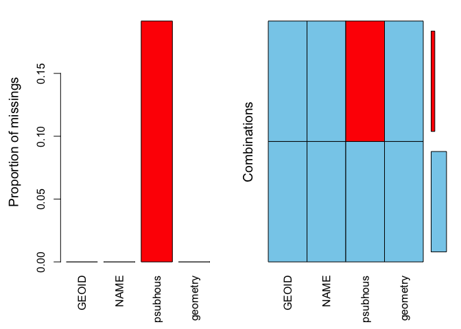
##
##  Missings per variable:
##  Variable Count
##     GEOID     0
##      NAME     0
##  psubhous    23
##  geometry     0
##
##  Missings in combinations of variables:
##  Combinations Count  Percent
##       0:0:0:0    97 80.83333
##       0:0:1:0    23 19.16667
The results show two tables and two plots. The left-hand side plot shows the proportion of cases that are missing values for each variable in the data set. The right-hand side plot shows which combinations of variables are missing. The first table shows the number of cases that are missing values for each variable in the data set. The second table shows the percent of cases missing values based on combinations of variables. The results show that 23 or 19% of census tracts are missing values on the variable psubhous.
Exclude missing data
The most simplest way for dealing with cases having missing values is to delete them. You do this using the filter() command
sac.city.tracts.sf.rm <- filter(sac.city.tracts.sf, is.na(psubhous) != TRUE)You now get your mean
sac.city.tracts.sf.rm %>% summarize(mean = mean(psubhous))## Simple feature collection with 1 feature and 1 field
## geometry type: POLYGON
## dimension: XY
## bbox: xmin: -121.5601 ymin: 38.43757 xmax: -121.3627 ymax: 38.68522
## epsg (SRID): 4269
## proj4string: +proj=longlat +datum=NAD83 +no_defs
## mean geometry
## 1 6.13866 POLYGON ((-121.409 38.50368...And your Moran’s I
#Turn sac.city.tracts.sf into an sp object.
sac.city.tracts.sp.rm <- as(sac.city.tracts.sf.rm, "Spatial")

sacb.rm<-poly2nb(sac.city.tracts.sp.rm, queen=T)
sacw.rm<-nb2listw(sacb.rm, style="W")
moran.test(sac.city.tracts.sp.rm$psubhous, sacw.rm)
##
## Moran I test under randomisation
##
## data: sac.city.tracts.sp.rm$psubhous
## weights: sacw.rm
##
## Moran I statistic standard deviate = 1.5787, p-value = 0.0572
## alternative hypothesis: greater
## sample estimates:
## Moran I statistic Expectation Variance
## 0.079875688 -0.010416667 0.003271021It’s often a better idea to keep your data intact rather than remove cases. For many of R’s functions, there is an na.rm = TRUE option, which tells R to remove all cases with missing values on the variable when performing the function. For example, inserting the na.rm = TRUE option in the mean() function yields
sac.city.tracts.sf %>% summarize(mean = mean(psubhous, na.rm=TRUE))## Simple feature collection with 1 feature and 1 field
## geometry type: POLYGON
## dimension: XY
## bbox: xmin: -121.5601 ymin: 38.43757 xmax: -121.3627 ymax: 38.6856
## epsg (SRID): 4269
## proj4string: +proj=longlat +datum=NAD83 +no_defs
## mean geometry
## 1 6.13866 POLYGON ((-121.409 38.50368...In the function moran.test(), we use the option na.action=na.omit
moran.test(sac.city.tracts.sp$psubhous, sacw, na.action=na.omit) ##
## Moran I test under randomisation
##
## data: sac.city.tracts.sp$psubhous
## weights: sacw
## omitted: 1, 2, 3, 17, 19, 21, 22, 23, 34, 43, 44, 46, 49, 50, 69, 74, 75, 99, 100, 101, 102, 106, 120
##
## Moran I statistic standard deviate = 1.5787, p-value = 0.0572
## alternative hypothesis: greater
## sample estimates:
## Moran I statistic Expectation Variance
## 0.079875688 -0.010416667 0.003271021Impute the mean
Usually, it is better to keep observations than discard or ignore them, especially if a large proportion of your sample is missing data. In the case of psubhous, were missing almost 20% of the data, which is a lot of cases to exclude. Moreover, not all functions have the built in na.rm or na.action options. Plus, look at this map
tm_shape(sac.city.tracts.sf.rm) + tm_polygons(col="blue")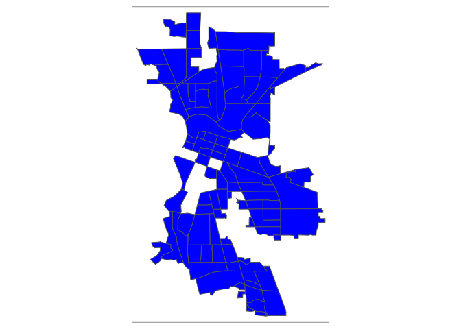
We’ve got permanent holes in Sacramento because we physically removed census tracts with missing values.
One way to keep observations with missing data is to impute a value for missingness. A simple imputation is the mean value of the variable. To impute the mean, we need to use the tidy friendly impute_mean() function in the tidyimpute package. Install this package and load it into R.
install.packages("tidyimpute")
library(tidyimpute)
Then use the function impute_mean(). To use this function, pipe in the data set and then type in the variables you want to impute.
sac.city.tracts.sf.mn <- sac.city.tracts.sf %>%
    impute_mean(psubhous)
Note that you can impute more than one variable within impute_mean() by separating variables with commas. We should now have no missing values
summary(aggr(sac.city.tracts.sf.mn))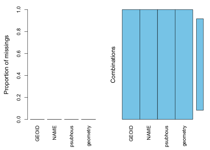
##
##  Missings per variable:
##  Variable Count
##     GEOID     0
##      NAME     0
##  psubhous     0
##  geometry     0
##
##  Missings in combinations of variables:
##  Combinations Count Percent
##       0:0:0:0   120     100
Therefore allowing us to calculate the mean of psubhous
sac.city.tracts.sf.mn %>% summarize(mean = mean(psubhous))## Simple feature collection with 1 feature and 1 field
## geometry type: POLYGON
## dimension: XY
## bbox: xmin: -121.5601 ymin: 38.43757 xmax: -121.3627 ymax: 38.6856
## epsg (SRID): 4269
## proj4string: +proj=longlat +datum=NAD83 +no_defs
## mean geometry
## 1 6.13866 POLYGON ((-121.409 38.50368...And a Moran’s I
#Turn sac.city.tracts.sf into an sp object.
sac.city.tracts.sp.mn <- as(sac.city.tracts.sf.mn, "Spatial")

sacb.mn<-poly2nb(sac.city.tracts.sp.mn, queen=T)
sacw.mn<-nb2listw(sacb.mn, style="W")
moran.test(sac.city.tracts.sp.mn$psubhous, sacw.mn)
##
## Moran I test under randomisation
##
## data: sac.city.tracts.sp.mn$psubhous
## weights: sacw.mn
##
## Moran I statistic standard deviate = 1.8814, p-value = 0.02996
## alternative hypothesis: greater
## sample estimates:
## Moran I statistic Expectation Variance
## 0.081778772 -0.008403361 0.002297679And our map has no holes!!
tmap_mode("view")
tm_shape(sac.city.tracts.sf.mn) +
  tm_polygons(col = "psubhous", style = "quantile")
Other Imputation Methods
The tidyimpute package has a set of functions for imputing missing values in your data. The functions are categorized as univariate and multivariate, where the former imputes a single value for all missing observations (like the mean) whereas the latter imputes a value based on a set of non-missing characteristics. Univariate methods include
impute_max— maximumimpute_minimum— minimumimpute_median— median valueimpute_quantile— quantile valueimpute_sample— randomly sampled value via bootstrap
Multivariate methods include
impute_fit,impute_predict— use a regression model to predict the valueimpute_by_group— use by-group imputation
Some of the multivariate functions may not be fully developed at the moment, but their test versions may be available for download. If you’re looking to use a multivariate method to impute missingness, check the Hmisc and MICE packages.
The MICE package provides functions for imputing missing values using multiple imputation methods. These methods take into account the uncertainty related to the unknown real values by imputing M plausible values for each unobserved response in the data. This renders M different versions of the data set, where the non-missing data is identical, but the missing data entries differ. These methods go beyond the scope of this class, but you can check a number of user created vignettes, include this, this and this. I’ve also uploaded onto Canvas (Additional Readings folder) a chapter from Gelman and Hill that covers missing data.
Website created and maintained by Noli Brazil