Содержание
- Основы Maple
- Декларации об ошибках
- Как исправить: ошибка в plot.window(…): нужны конечные значения «xlim»
- Пример 1: Ошибка с вектором символов
- Пример 2: Ошибка с вектором значений NA
- Дополнительные ресурсы
- Plotting means and error bars (ggplot2)
- Problem
- Solution
- Sample data
- Line graphs
- Bar graphs
- Error bars for within-subjects variables
- One within-subjects variable
- Understanding within-subjects error bars
- Two within-subjects variables
- Note about normed means
- Helper functions
- R Error in plot.window(…) : need finite ‘xlim’ values (2 Examples)
- Creation of Example Data
- Example 2: Avoid the Error Message – need finite ‘xlim’ values
- Exponenta.ru
- не могу понять в чем ошибка. помогите пожалуйста!!
- не могу понять в чем ошибка. помогите пожалуйста!!
- Re: не могу понять в чем ошибка. помогите пожалуйста!!
Основы Maple

Декларации об ошибках
- Если получен неожиданный ответ, то зачастую причина в том, что Maple понимает переменную иначе, чем вы хотели бы ее представить. Например, полагая, что х – только число, можно легко ошибиться, поскольку на самом деле оказывается, что х – это переменная. Исправить можно так:
тогда Maple представит себе переменные х и у должным образом. Учтите, что попытка заставить Maple выдать числа, применяя assume к переменной, может создать проблему.
- Посмотрите, где находится первый пробел в команде, например, не стоит ли между знаком > и первым символом команды. Уберите этот пробел.
- Если проблеме не исчезла, сотрите полностью строку и перенаберите ее заново.
emptyplot (пустой график).
Причина: синтаксическая ошибка при построении выражений.
axes appear, but no function is plotted (есть только оси координат, но нет графика).
Так получается, если неправильно заданы параметры осей графика.
Error, (in plot) invalid arguments (Ошибка, (в графике) неверные аргументы).
Возможно, вы пытаетесь построить график с переменной, которой было присвоено значение.
Error, (in plot/transform) can not evaluate boolean: –5.*z = вместо := .
Parametric plot gives two plots instead (Выдаются два графика вместо параметрического графика).
Это случается, если неправильно поставлены скобки [ ] .
Function plotting fails (График функции не получился).
Не удается построить график только что определенной функции f(x) с помощью plot(f(x),x=0..5) . Проверьте, что находится в переменной, содержащей f(x).
Error, wrong number (or type) of parameters in function diff (Ошибка, неверное количество или тип параметров в функции diff).
То же, что и в проблеме неприсваивания при построении графиков (см. выше), но только для diff .
Нужно применить unassign x (не забудьте применить кавычки):
Error, (in int) wrong number (or type) of arguments (Ошибка, (в int) неправильное число (или тип аргументов)).
То же, что и в неприсваивании при построении графиков (см выше), но только для int .
Нужно применить unassign x (не забудьте использовать кавычки):
Nothing comes back (нет ответа).
Иногда Maple может решить систему, если коэффициенты являются рациональными числами, и не может, если они являются числами с плавающей точкой. Поэтому не используйте x*0.01 – вместо этого используйте x/100.
Error, too many levels of recursion or Warning, recursive definition of name (Ошибка, слишком много уровней рекурсии или Предупреждение, рекурсивное определение имени).
You want x to be a variable, but it is a number instead (Вы хотите, чтобы х был переменной, но на самом деле – это число).
Ранее x было присвоено значение, а нужна переменная.
Это иной путь «расприсваивания» переменной.
Error, (in assign) invalid arguments (Ошибка,(в присваивании) неверные аргументы).
Источник
Как исправить: ошибка в plot.window(…): нужны конечные значения «xlim»
Одна ошибка, с которой вы можете столкнуться при использовании R:
Эта ошибка возникает, когда вы пытаетесь создать график в R и используете либо вектор символов, либо вектор только со значениями NA на оси x.
В следующих примерах показаны два разных сценария, в которых эта ошибка может возникнуть на практике.
Пример 1: Ошибка с вектором символов
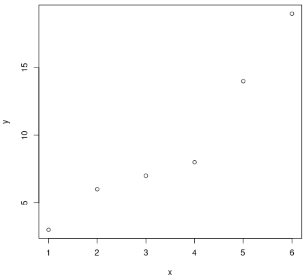
Предположим, вы пытаетесь создать диаграмму рассеяния, используя следующий код:
Мы получаем ошибку, потому что вектор, который мы использовали для значений оси x, является вектором символов.
Чтобы исправить эту ошибку, нам просто нужно указать числовой вектор по оси X:

Мы можем создать диаграмму рассеяния без каких-либо ошибок, потому что мы предоставили числовой вектор для оси X.
Пример 2: Ошибка с вектором значений NA
Предположим, вы пытаетесь создать диаграмму рассеяния, используя следующий код:
Мы получаем ошибку, потому что вектор, который мы использовали для значений по оси x, является вектором только со значениями NA.
Чтобы исправить эту ошибку, нам просто нужно указать числовой вектор по оси X:

И снова мы можем успешно создать диаграмму рассеяния без ошибок, потому что мы использовали числовой вектор для оси x.
Дополнительные ресурсы
В следующих руководствах объясняется, как исправить другие распространенные ошибки в R:
Источник
Plotting means and error bars (ggplot2)
Problem
You want to plot means and error bars for a dataset.
Solution
To make graphs with ggplot2, the data must be in a data frame, and in “long” (as opposed to wide) format. If your data needs to be restructured, see this page for more information.
Sample data
The examples below will the ToothGrowth dataset. Note that dose is a numeric column here; in some situations it may be useful to convert it to a factor.
First, it is necessary to summarize the data. This can be done in a number of ways, as described on this page. In this case, we’ll use the summarySE() function defined on that page, and also at the bottom of this page. (The code for the summarySE function must be entered before it is called here).
Line graphs
After the data is summarized, we can make the graph. These are basic line and point graph with error bars representing either the standard error of the mean, or 95% confidence interval.
/figure/unnamed-chunk-4-1.png)
/figure/unnamed-chunk-4-2.png)
/figure/unnamed-chunk-4-3.png)
/figure/unnamed-chunk-4-4.png)
A finished graph with error bars representing the standard error of the mean might look like this. The points are drawn last so that the white fill goes on top of the lines and error bars.
/figure/unnamed-chunk-5-1.png)
Bar graphs
The procedure is similar for bar graphs. Note that tgc$size must be a factor. If it is a numeric vector, then it will not work.
/figure/unnamed-chunk-6-1.png)
/figure/unnamed-chunk-6-2.png)
A finished graph might look like this.
/figure/unnamed-chunk-7-1.png)
Error bars for within-subjects variables
When all variables are between-subjects, it is straightforward to plot standard error or confidence intervals. However, when there are within-subjects variables (repeated measures), plotting the standard error or regular confidence intervals may be misleading for making inferences about differences between conditions.
The method below is from Morey (2008), which is a correction to Cousineau (2005), which in turn is meant to be a simpler method of that in Loftus and Masson (1994). See these papers for a more detailed treatment of the issues involved in error bars with within-subjects variables.
One within-subjects variable
Here is a data set (from Morey 2008) with one within-subjects variable: pre/post-test.
The first step is to convert it to long format. See this page for more information about the conversion.
Collapse the data using summarySEwithin (defined at the bottom of this page; both of the helper functions below must be entered before the function is called here).
/figure/unnamed-chunk-10-1.png)
The value and value_norm columns represent the un-normed and normed means. See the section below on normed means for more information.
Understanding within-subjects error bars
This section explains how the within-subjects error bar values are calculated. The steps here are for explanation purposes only; they are not necessary for making the error bars.
The graph of individual data shows that there is a consistent trend for the within-subjects variable condition , but this would not necessarily be revealed by taking the regular standard errors (or confidence intervals) for each group. The method in Morey (2008) and Cousineau (2005) essentially normalizes the data to remove the between-subject variability and calculates the variance from this normalized data.
/figure/unnamed-chunk-11-1.png)
/figure/unnamed-chunk-11-2.png)
The differences in the error bars for the regular (between-subject) method and the within-subject method are shown here. The regular error bars are in red, and the within-subject error bars are in black.
/figure/unnamed-chunk-12-1.png)
Two within-subjects variables
If there is more than one within-subjects variable, the same function, summarySEwithin , can be used. This data set is taken from Hays (1994), and used for making this type of within-subject error bar in Rouder and Morey (2005).
The data must first be converted to long format. In this case, the column names indicate two variables, shape (round/square) and color scheme (monochromatic/colored).
Now it can be summarized and graphed.
/figure/unnamed-chunk-15-1.png)
Note about normed means
The summarySEWithin function returns both normed and un-normed means. The un-normed means are simply the mean of each group. The normed means are calculated so that means of each between-subject group are the same. These values can diverge when there are between-subject variables.
Helper functions
The summarySE function is also defined on this page. If you only are working with between-subjects variables, that is the only function you will need in your code. If you have within-subjects variables and want to adjust the error bars so that inter-subject variability is removed as in Loftus and Masson (1994), then the other two functions, normDataWithin and summarySEwithin must also be added to your code; summarySEwithin will then be the function that you call.
Источник
R Error in plot.window(…) : need finite ‘xlim’ values (2 Examples)
This article illustrates how to handle the plot error “need finite ‘xlim’ values” in R.
Table of contents:
Let’s dive into it…
Creation of Example Data
As a first step, we need to create some example data. First, we’ll create an x-vector:
x Example 1: Reproduce the Error Message – need finite ‘xlim’ values
In this example, I’ll illustrate how to replicate the error message “need finite ‘xlim’ values” in R.
If we want to draw our previously created data to a plot, we might try to use the following R code:
plot(x, y) # Try to draw plot # Error in plot.window(. ) : need finite ‘xlim’ values # In addition: Warning messages: # 1: In min(x) : no non-missing arguments to min; returning Inf # 2: In max(x) : no non-missing arguments to max; returning -Inf
As you can see, the previous syntax returned the error message “need finite ‘xlim’ values”.
That’s obviously no surprise. Our x vector contains only missing values and hence cannot be drawn to a plot.
So how can we solve this problem?
Example 2: Avoid the Error Message – need finite ‘xlim’ values
In Example 2, I’ll show how to fix the problems with the error message “need finite ‘xlim’ values”.
First, we have to create an x vector that contains actual values:
x2 Video & Further Resources
Have a look at the following video of my YouTube channel. I illustrate the R programming code of this article in the video:
Please accept YouTube cookies to play this video. By accepting you will be accessing content from YouTube, a service provided by an external third party.

If you accept this notice, your choice will be saved and the page will refresh.
Accept YouTube Content
In addition, you may want to read the other posts of my homepage. I have released numerous tutorials about topics such as labels and graphics in R:
At this point in the article you should know how to deal with the plotting error message “need finite ‘xlim’ values” in the R programming language.
Please note that a very similar error message could occur, in case all y-values are NA (i.e. “Error in plot.window(…) : need finite ‘ylim’ values”).
Don’t hesitate to tell me about it in the comments, in case you have any additional questions.
Источник
Exponenta.ru
Образовательный математический сайт
не могу понять в чем ошибка. помогите пожалуйста!!
Модератор: Admin
не могу понять в чем ошибка. помогите пожалуйста!!
Сообщение Nata117 » Вт янв 11, 2011 11:59 am
Re: не могу понять в чем ошибка. помогите пожалуйста!!
Сообщение Kitonum » Вт янв 11, 2011 7:01 pm
Сообщение Nata117 » Ср янв 12, 2011 12:15 pm
Сообщение Kitonum » Ср янв 12, 2011 2:14 pm
В одном из Ваших уравнений присутствует параметр p , значение которого не определено. Это — основная причина, почему не считается! Ну ещё те ошибки, о которых я уже писал. Я произвольно присвоил p значение 1 , после чего всё заработало!
Фрагмент кода:
p:=1: Sp:=map(res,[seq(0.09/50*i,i=0..50)]);
Sp := [[t = 0., P(t) = 50., phi(t) = 1.], [t = .1800000000e-2, P(t) = 50.4350063251672012, phi(t) = .975968257705710384], [t = .3600000000e-2, P(t) = 50.9177946569956532, phi(t) = .952154283567009596], [t = .5400000000e-2, P(t) = 51.4442649641215724, phi(t) = .928575262186644434], [t = .7200000000e-2, P(t) = 52.0100685458456198, phi(t) = .905245332470889120], [t = .9000000000e-2, P(t) = 52.6107447398945710, phi(t) = .882175672502904851], [t = .1080000000e-1, P(t) = 53.2418274517322346, phi(t) = .859374639670642426], [t = .1260000000e-1, P(t) = 53.8988825218068898, phi(t) = .836847924424685808], [t = .1440000000e-1, P(t) = 54.5775990481969658, phi(t) = .814598703439283200], [t = .1620000000e-1, P(t) = 55.2738513461950376, phi(t) = .792628066493929473], [t = .1800000000e-1, P(t) = 55.9837238824985662, phi(t) = .770935261014395912], [t = .1980000000e-1, P(t) = 56.7035233445178904, phi(t) = .749517887104383052], [t = .2160000000e-1, P(t) = 57.4298265157117669, phi(t) = .728371944480206146], [t = .2340000000e-1, P(t) = 58.1594664180973808, phi(t) = .707492352371674072], [t = .2520000000e-1, P(t) = 58.8895239747403778, phi(t) = .686873227308512968], [t = .2700000000e-1, P(t) = 59.6173271958009536, phi(t) = .666507891832906818], [t = .2880000000e-1, P(t) = 60.3404453593376076, phi(t) = .646389042795666002], [t = .3060000000e-1, P(t) = 61.0567034955123376, phi(t) = .626508763596743234], [t = .3240000000e-1, P(t) = 61.7641275239122366, phi(t) = .606858907189038344], [t = .3420000000e-1, P(t) = 62.4609315063902956, phi(t) = .587431197213856504], [t = .3600000000e-1, P(t) = 63.1455176385617847, phi(t) = .568217228028420674], [t = .3780000000e-1, P(t) = 63.8164629067057306, phi(t) = .549208502542908648], [t = .3960000000e-1, P(t) = 64.4725167587298956, phi(t) = .530396440458462681], [t = .4140000000e-1, P(t) = 65.1125679470279550, phi(t) = .511772527622042728], [t = .4320000000e-1, P(t) = 65.7356236318277354, phi(t) = .493328392111318182], [t = .4500000000e-1, P(t) = 66.3408093811911215, phi(t) = .475055804234666646], [t = .4680000000e-1, P(t) = 66.9273642822145406, phi(t) = .456946676681127650], [t = .4860000000e-1, P(t) = 67.4946293389597828, phi(t) = .438993036225981348], [t = .5040000000e-1, P(t) = 68.0420435093492699, phi(t) = .421187056400741888], [t = .5220000000e-1, P(t) = 68.5691159771347004, phi(t) = .403521114066910158], [t = .5400000000e-1, P(t) = 69.0754246280541224, phi(t) = .385987791226163778], [t = .5580000000e-1, P(t) = 69.5606160498319498, phi(t) = .368579875020357938], [t = .5760000000e-1, P(t) = 70.0244006116413118, phi(t) = .351290346461309910], [t = .5940000000e-1, P(t) = 70.4665459721530994, phi(t) = .334112333550809937], [t = .6120000000e-1, P(t) = 70.8868763438969866, phi(t) = .317039141370691724], [t = .6300000000e-1, P(t) = 71.2852549918250986, phi(t) = .300064257729813821], [t = .6480000000e-1, P(t) = 71.6615836658388190, phi(t) = .283181352704035660], [t = .6660000000e-1, P(t) = 72.0158026007892431, phi(t) = .266384278636218718], [t = .6840000000e-1, P(t) = 72.3478904868938742, phi(t) = .249667070020255288], [t = .7020000000e-1, P(t) = 72.6578581709716360, phi(t) = .233023906342104431], [t = .7200000000e-1, P(t) = 72.9457505912858154, phi(t) = .216449094140738652], [t = .7380000000e-1, P(t) = 73.2116411716993128, phi(t) = .199937087194482720], [t = .7560000000e-1, P(t) = 73.4556259872405946, phi(t) = .183482473988763079], [t = .7740000000e-1, P(t) = 73.6778237641035930, phi(t) = .167079977716107774], [t = .7920000000e-1, P(t) = 73.8783758796477628, phi(t) = .150724456276146668], [t = .8100000000e-1, P(t) = 74.0574463623980250, phi(t) = .134410902275611366], [t = .8280000000e-1, P(t) = 74.2152205650808128, phi(t) = .118134427378747742], [t = .8460000000e-1, P(t) = 74.3519027987358072, phi(t) = .101890218433768012], [t = .8640000000e-1, P(t) = 74.4677170575893684, phi(t) = .856735713709563806e-1], [t = .8820000000e-1, P(t) = 74.5629034094364728, phi(t) = .694798767283690972e-1], [t = .9000000000e-1, P(t) = 74.6377178645699360, phi(t) = .533046185895388186e-1]]
Источник
There is no help page available for this error
Sorry, we do not have specific information about your error. There are several resources that can help you find a solution:
Related Maplesoft Help Pages
-
12 Graphics
Contents Previous Next Index 12 Graphics Maple offers a variety of ways to generate
2-D and 3-D plots. This chapter shows you how to create and manipulate such … -
6 Procedures
Contents Previous Next Index 6 Procedures A Maple procedure is a sequence of parameter
declarations, variable declarations, and statements that encapsulates a computation … -
Interpolation and Smoothing
Interpolated Plotting and Smoothing in Maple 16 The topic of this worksheet is
interpolation and smoothing of given 2-dimensional and 3-dimensional data. The …
Related Posts & Questions on MaplePrimes
-
I am getting the error in plot — MaplePrimes
Sep 13, 2015 … plot([Y2(t),-X2(t),0…100],numpoints=100);. Error, (in plot) procedure expected, as range contains no plotting variable … -
how I solve a Hard Triple Integral? — MaplePrimes
Nov 9, 2019 … 200. (1) ;.3. (2) ; Error, (in plot) procedure expected, as range contains no plotting variable ;.3798. (3) ;.22788. (4) … -
how to PLOT PDE IBCS for different Sc , Pr, Gr, Gm at fixed t? Also …
Mar 10, 2018 … Error, (in plot/options2d) unexpected option: .22 = .1 … Error, (in plot) procedure expected, as range contains no plotting variable …
Other Resources
- Review the Error Message Guide Overview
- Frequently Asked Questions
- Contact Maplesoft Technical Support
|
0 / 0 / 0 Регистрация: 10.01.2016 Сообщений: 9 |
|
|
1 |
|
Почему график пустой и выводит предупреждение03.05.2016, 15:44. Показов 3241. Ответов 11
Добрый день! Помогите разобраться, почему у меня график пустой, и выводит предупреждение? Впроде бы уже все проверила, не могу понять, что он хочет… Код на картинке: Миниатюры
__________________
0 |

|
Programming Эксперт 94731 / 64177 / 26122 Регистрация: 12.04.2006 Сообщений: 116,782 |
03.05.2016, 15:44 |
|
Ответы с готовыми решениями: Выводит пустой отчет FastReport6 Выводит пустой отчет Как создать пустой график Подскажите, почему не запускается и почему не выводит решение по частям? 11 |
|
Модератор
5031 / 3862 / 1327 Регистрация: 30.07.2012 Сообщений: 11,435 |
|
|
03.05.2016, 16:25 |
2 |
|
Код на картинке: Код должен быть в ФАЙЛЕ, а не на картинке…
0 |

 Прикрепите архив своего файла.
|
0 / 0 / 0 Регистрация: 10.01.2016 Сообщений: 9 |
|
|
03.05.2016, 16:43 [ТС] |
3 |
|
извините, вот файл:
0 |
|
19 / 19 / 2 Регистрация: 15.05.2011 Сообщений: 142 |
|
|
03.05.2016, 19:14 |
4 |
|
у меня график пустой, и выводит предупреждение? А у меня в вашем файле все построило. Миниатюры
0 |
|
Модератор
5031 / 3862 / 1327 Регистрация: 30.07.2012 Сообщений: 11,435 |
|
|
03.05.2016, 19:17 |
5 |
|
Акаша, у меня график строится… Maple 2015 Миниатюры
0 |
|
0 / 0 / 0 Регистрация: 10.01.2016 Сообщений: 9 |
|
|
03.05.2016, 19:28 [ТС] |
6 |
|
у меня Maple14, такое чувство, что через раз он графики строит( VSI,
0 |
|
19 / 19 / 2 Регистрация: 15.05.2011 Сообщений: 142 |
|
|
04.05.2016, 23:44 |
7 |
|
установила maple15 15? Не 2015? Просто есть Maple 15 и есть Maple 2015, и между ними 4 года разницы в выпуске)
0 |
|
0 / 0 / 0 Регистрация: 10.01.2016 Сообщений: 9 |
|
|
08.05.2016, 13:15 [ТС] |
8 |
|
15? Не 2015? Просто есть Maple 15 и есть Maple 2015, и между ними 4 года разницы в выпуске) Maple 2015 korsar-pirat, извините, но тут действительно какая-то ерунда получается: Я поняла в чем проблема, каждый раз при открытии файла, если хочешь продолжать что-то в нем и дальше писать, прежде нужно пересчитать все предыдущие формулы, и только после этого писать новые, т.к. если этого не сделать графики что последующие, что новые строятся пустые.
0 |
|
19 / 19 / 2 Регистрация: 15.05.2011 Сообщений: 142 |
|
|
08.05.2016, 15:37 |
9 |
|
Кажется логично, если переменные пустые, а вы хотите построить график.
1 |
|
0 / 0 / 0 Регистрация: 10.01.2016 Сообщений: 9 |
|
|
09.05.2016, 13:24 [ТС] |
10 |
|
korsar-pirat, Вот а сейчас , что с ним не так? вроде сделала все как в методичке, прогнала файл уже раз 10 , но два последних графика пустые… вообще не понимаю, почему так.
0 |
|
19 / 19 / 2 Регистрация: 15.05.2011 Сообщений: 142 |
|
|
09.05.2016, 16:43 |
11 |
|
но два последних графика пустые… проблема с bkf4. Миниатюры
0 |
|
0 / 0 / 0 Регистрация: 10.01.2016 Сообщений: 9 |
|
|
09.05.2016, 17:19 [ТС] |
12 |
|
korsar-pirat, да, действительно пропустила переменные. спасибо большое!
0 |
|
IT_Exp Эксперт 87844 / 49110 / 22898 Регистрация: 17.06.2006 Сообщений: 92,604 |
09.05.2016, 17:19 |
|
12 |
Основы Maple
Декларации об ошибках
- Если получен неожиданный ответ, то зачастую причина в том, что Maple понимает переменную иначе, чем вы хотели бы ее представить. Например, полагая, что х – только число, можно легко ошибиться, поскольку на самом деле оказывается, что х – это переменная. Исправить можно так:
тогда Maple представит себе переменные х и у должным образом. Учтите, что попытка заставить Maple выдать числа, применяя assume к переменной, может создать проблему.
- Посмотрите, где находится первый пробел в команде, например, не стоит ли между знаком > и первым символом команды. Уберите этот пробел.
- Если проблеме не исчезла, сотрите полностью строку и перенаберите ее заново.
emptyplot (пустой график).
Причина: синтаксическая ошибка при построении выражений.
axes appear, but no function is plotted (есть только оси координат, но нет графика).
Так получается, если неправильно заданы параметры осей графика.
Error, (in plot) invalid arguments (Ошибка, (в графике) неверные аргументы).
Возможно, вы пытаетесь построить график с переменной, которой было присвоено значение.
Error, (in plot/transform) can not evaluate boolean: –5.*z = вместо := .
Parametric plot gives two plots instead (Выдаются два графика вместо параметрического графика).
Это случается, если неправильно поставлены скобки [ ] .
Function plotting fails (График функции не получился).
Не удается построить график только что определенной функции f(x) с помощью plot(f(x),x=0..5) . Проверьте, что находится в переменной, содержащей f(x).
Error, wrong number (or type) of parameters in function diff (Ошибка, неверное количество или тип параметров в функции diff).
То же, что и в проблеме неприсваивания при построении графиков (см. выше), но только для diff .
Нужно применить unassign x (не забудьте применить кавычки):
Error, (in int) wrong number (or type) of arguments (Ошибка, (в int) неправильное число (или тип аргументов)).
То же, что и в неприсваивании при построении графиков (см выше), но только для int .
Нужно применить unassign x (не забудьте использовать кавычки):
Nothing comes back (нет ответа).
Иногда Maple может решить систему, если коэффициенты являются рациональными числами, и не может, если они являются числами с плавающей точкой. Поэтому не используйте x*0.01 – вместо этого используйте x/100.
Error, too many levels of recursion or Warning, recursive definition of name (Ошибка, слишком много уровней рекурсии или Предупреждение, рекурсивное определение имени).
You want x to be a variable, but it is a number instead (Вы хотите, чтобы х был переменной, но на самом деле – это число).
Ранее x было присвоено значение, а нужна переменная.
Это иной путь «расприсваивания» переменной.
Error, (in assign) invalid arguments (Ошибка,(в присваивании) неверные аргументы).
Источник
Error in plot procedure expected as range contains no plotting variable
I noticed this package is not introduced in Maple 17.. what is the alternative way to produce smother curve
limit of the integral is function.
The integration in (F2) is not work properly.
My tyr is below:
b:=-gamma1*tau0+I*tau0*Delta-2*a*(k-1)*xr:
a:=1+I*c;
c1:=sqrt(conjugate(a))/tau0:
c2:=0.5*((conjugate(b)/sqrt(conjugate(a)))):
lambda1:=2*(1-I*d)*(t-k1)/j+(1-I*d)^2:
lambda2:=t*(1-j)*k1/j+1/sqrt(2)*(1-I*d):
lambda3:=c1*(t-k1)/j+c1*(1-I*d)+c2:
J1:=sqrt(Pi)/sqrt(2)*(1-erf(lambda2)):
J1mod:=(Re(J1))^2+(Im(J1))^2:
g1:=0.5*sqrt(Pi)*tau0*exp(c2^2)*exp(-conjugate(a)*((k-1)*xr)^2)/(sqrt(conjugate(a))):
F2:=-sqrt(2)*int(exp(-x^2)*erf(sqrt(2)*c1*x+lambda3),x=-lambda2..infty);
Warning, computation interrupted
J2:=sum(g1*J1+g1*F2,k=1..1);
J2mod:=(((Re(J2))^2+(Im(J2))^2)):
W:= unapply(no*J1mod+Omega^2*J2mod,d):
Omega:=0.01:no:=1:Delta:=0:tau0:=1:c:=0:gamma1:=0:j:=1:k1:=0:t:=2*Pi:xr:=1:
P1:=plot(W,-50..50,axes=boxed,title=tit,color=black,font=[2,3,18],thickness=2,tickmarks=[3,2],titlefont=[SYMBOL,14],font=[1,1,18],linestyle=1);
| From: |
| To: |
| Custom Message (optional): |
You must be logged into your Facebook account in order to share via Facebook.
Login to Facebook
Click the button below to share this on Google+. A new window will open.
Click Here to Share on Google+
You must be logged in to your Twitter account in order to share. Click the button below to login (a new window will open.)
Источник
Как исправить: ошибка в plot.window(…): нужны конечные значения «xlim»
Одна ошибка, с которой вы можете столкнуться при использовании R:
Эта ошибка возникает, когда вы пытаетесь создать график в R и используете либо вектор символов, либо вектор только со значениями NA на оси x.
В следующих примерах показаны два разных сценария, в которых эта ошибка может возникнуть на практике.
Пример 1: Ошибка с вектором символов
Предположим, вы пытаетесь создать диаграмму рассеяния, используя следующий код:
Мы получаем ошибку, потому что вектор, который мы использовали для значений оси x, является вектором символов.
Чтобы исправить эту ошибку, нам просто нужно указать числовой вектор по оси X:
Мы можем создать диаграмму рассеяния без каких-либо ошибок, потому что мы предоставили числовой вектор для оси X.
Пример 2: Ошибка с вектором значений NA
Предположим, вы пытаетесь создать диаграмму рассеяния, используя следующий код:
Мы получаем ошибку, потому что вектор, который мы использовали для значений по оси x, является вектором только со значениями NA.
Чтобы исправить эту ошибку, нам просто нужно указать числовой вектор по оси X:
И снова мы можем успешно создать диаграмму рассеяния без ошибок, потому что мы использовали числовой вектор для оси x.
Дополнительные ресурсы
В следующих руководствах объясняется, как исправить другие распространенные ошибки в R:
Источник
Plotting means and error bars (ggplot2)
Problem
You want to plot means and error bars for a dataset.
Solution
To make graphs with ggplot2, the data must be in a data frame, and in “long” (as opposed to wide) format. If your data needs to be restructured, see this page for more information.
Sample data
The examples below will the ToothGrowth dataset. Note that dose is a numeric column here; in some situations it may be useful to convert it to a factor.
First, it is necessary to summarize the data. This can be done in a number of ways, as described on this page. In this case, we’ll use the summarySE() function defined on that page, and also at the bottom of this page. (The code for the summarySE function must be entered before it is called here).
Line graphs
After the data is summarized, we can make the graph. These are basic line and point graph with error bars representing either the standard error of the mean, or 95% confidence interval.
A finished graph with error bars representing the standard error of the mean might look like this. The points are drawn last so that the white fill goes on top of the lines and error bars.
Bar graphs
The procedure is similar for bar graphs. Note that tgc$size must be a factor. If it is a numeric vector, then it will not work.
A finished graph might look like this.
Error bars for within-subjects variables
When all variables are between-subjects, it is straightforward to plot standard error or confidence intervals. However, when there are within-subjects variables (repeated measures), plotting the standard error or regular confidence intervals may be misleading for making inferences about differences between conditions.
The method below is from Morey (2008), which is a correction to Cousineau (2005), which in turn is meant to be a simpler method of that in Loftus and Masson (1994). See these papers for a more detailed treatment of the issues involved in error bars with within-subjects variables.
One within-subjects variable
Here is a data set (from Morey 2008) with one within-subjects variable: pre/post-test.
The first step is to convert it to long format. See this page for more information about the conversion.
Collapse the data using summarySEwithin (defined at the bottom of this page; both of the helper functions below must be entered before the function is called here).
The value and value_norm columns represent the un-normed and normed means. See the section below on normed means for more information.
Understanding within-subjects error bars
This section explains how the within-subjects error bar values are calculated. The steps here are for explanation purposes only; they are not necessary for making the error bars.
The graph of individual data shows that there is a consistent trend for the within-subjects variable condition , but this would not necessarily be revealed by taking the regular standard errors (or confidence intervals) for each group. The method in Morey (2008) and Cousineau (2005) essentially normalizes the data to remove the between-subject variability and calculates the variance from this normalized data.
The differences in the error bars for the regular (between-subject) method and the within-subject method are shown here. The regular error bars are in red, and the within-subject error bars are in black.
Two within-subjects variables
If there is more than one within-subjects variable, the same function, summarySEwithin , can be used. This data set is taken from Hays (1994), and used for making this type of within-subject error bar in Rouder and Morey (2005).
The data must first be converted to long format. In this case, the column names indicate two variables, shape (round/square) and color scheme (monochromatic/colored).
Now it can be summarized and graphed.
Note about normed means
The summarySEWithin function returns both normed and un-normed means. The un-normed means are simply the mean of each group. The normed means are calculated so that means of each between-subject group are the same. These values can diverge when there are between-subject variables.
Helper functions
The summarySE function is also defined on this page. If you only are working with between-subjects variables, that is the only function you will need in your code. If you have within-subjects variables and want to adjust the error bars so that inter-subject variability is removed as in Loftus and Masson (1994), then the other two functions, normDataWithin and summarySEwithin must also be added to your code; summarySEwithin will then be the function that you call.
Источник
R error in plot.window(. ) need finite ‘xlim’ values
I want to plot a data.frame and my problem is, that the following error appears:
This is my code:
I thought the problem might be, that x and y are character values and this cannot be plotted (x are dates and times for example 16.06.2015 20:07:00 and y just a double value like 0,0300 ). But I couldn’t really do y = as.numeric(CO2.data$V2) because then every value was NA.
The result of str(CO2.data) is:
1 Answer 1
But I couldn’t really do y = as.numeric(CO2.data$V2) because then every value was NA.
Well plot essentially has the same problem.
When reading in data, the first step should always be to put the data into an appropriate format, and only then process to the next step. Your workflow should always look like this, with virtually no exceptions.
In your case, you need to convert the datetime and the numeric values explicitly because R cannot handle the format conversion automatically:
In particular, you need to specify the date format (first line) and you need to convert decimal commas into decimal points before converting the strings to numbers.
If you use read.csv2 instead of read.table , you can specify the decimal separator; this allows you to omit the second conversion above:
Oh, and use FALSE and TRUE , not F and T — the latter are variables, so some code could redefine the meaning of F and T .
Источник
You should upgrade or use an alternative browser.
-
Forums
-
Mathematics
-
MATLAB, Maple, Mathematica, LaTeX
Maple — Error (in plots:-display)
- Maple
-
Thread starter
darida -
Start date
Oct 1, 2013 -
-
Tags -
maple
-
- Oct 1, 2013
- #1
eps1 := [0, 1/5, 2/5, 3/5, 4/5, 1]:
start1 := 2.3:
base1 := 1.1:
for i from 1 to 6 do
R := start1*base1**0:
points1 := [R, evalf(eval(mH, {M=1, r=R, epsilon = eps1}))]:
for a from 1 to 20 do
R := start1*base1**a:
points1 := points1, [R, evalf(eval(mH, {M=1, r=R, epsilon = eps1}))]:
end do:
end do:
plots[display]({
setoptions(symbol = diamond, symbolsize = 12, color = black),
plot([points1[1]]), pointplot([points1[1]]),
plot([points1[2]]), pointplot([points1[2]]),
plot([points1[3]]), pointplot([points1[3]]),
plot([points1[4]]), pointplot([points1[4]]),
plot([points1[5]]), pointplot([points1[5]]),
plot([points1[6]]), pointplot([points1[6]]),
},
textplot({[16,1.0, epsilon_ = 0.0],[16, 0.95, epsilon_ = 0.2],
[16, 0.84, epsilon_ = 0.4],[16, 0.95, epsilon_ = 0.6],
[16, 0.5, epsilon_ = 0.8],[16, 0.29, epsilon_ = 1.0]},
align={right},font=[TIMES,ROMAN,12]),
axes=boxed,
axis[1] = [mode = log, gridlines = [8, thickness = 1, subticks = false, color = grey]],
axis[2] = [gridlines = [color = grey]],
view = [2 .. 16, .25 .. 1.03]
);
But got this error:
Error, (in plots:-display) cannot make plot structure from object with name pointplot
What is wrong here?
Source: «www.diva-portal.org/smash/get/diva2:114136/FULLTEXT01.pdf» [Broken]
Edit: Appendix A
Answers and Replies
Suggested for: Maple — Error (in plots:-display)
- Last Post
- Sep 15, 2022
- Last Post
- Sep 5, 2022
- Last Post
- Jan 9, 2021
- Last Post
- Oct 23, 2019
- Last Post
- May 12, 2020
- Last Post
- Sep 4, 2019
- Last Post
- Jan 18, 2021
- Last Post
- Apr 13, 2018
- Last Post
- Apr 8, 2018
- Last Post
- Sep 19, 2017
-
Forums
-
Mathematics
-
MATLAB, Maple, Mathematica, LaTeX
![]()

- Forum
- Futura-Sciences : les forums de la science
- MATHEMATIQUES
- Math�matiques du sup�rieur
- Maple 18

R�pondre � la discussion
Affichage des r�sultats 1 � 1 sur 1
-
06/06/2016, 13h34
#1
Maple 18
——
bonjour,
j’ai une fonction p�riode de 2pi suivante g=pi-x (pour x appartenant [0,pi])…
Je souhaite la tracer avec MAPLE 18, mais j’ai toujours une erreur.. o� est-elle? l’erreur intervient seulement sur le rept… mais laquelle?
voici ce j’ai:
restart; with(plots); libname := libname, currentdir();
g := piecewise(-Pi <= x and x < 0, Pi+x, 0 <= x and x <= Pi, Pi-x);
piecewise(-Pi <= x and x < 0, Pi + x, 0 <= x and x <= Pi, Pi — x)plot(rept(g, x = -Pi .. Pi), -2*Pi .. 2*Pi, color = red, thickness = 2);
Error, (in plot) procedure expected, as range contains no plotting variable
Merci,
——
Discussions similaires
-
R�ponses: 3
Dernier message: 16/03/2014, 00h31
-
Maple
Par Astroide dans le forum Logiciel — Software — Open Source
R�ponses: 12
Dernier message: 11/09/2008, 23h46
-
R�ponses: 4
Dernier message: 09/08/2007, 18h55
-
maple IV
Par sadyoner dans le forum Math�matiques du sup�rieur
R�ponses: 3
Dernier message: 01/11/2006, 15h58
-
Maple
Par alleunam dans le forum Math�matiques du sup�rieur
R�ponses: 13
Dernier message: 14/07/2006, 11h03
Fuseau horaire GMT +1. Il est actuellement 15h01.
Still seeing an error with the updated version of GDAL. Printing the session_info() also, in case that helps:
library(sf)
#> Linking to GEOS 3.7.0, GDAL 2.3.2, PROJ 5.2.0
u = "https://github.com/geocompr/geocompkg/releases/download/0.1/munster.gpx"
download.file(url = u, destfile = "munster.gpx")
st_layers(f)
#> Error in st_layers(f): object 'f' not found
r_munster = read_sf(u, "tracks")
#> Warning in CPL_read_ogr(dsn, layer, query, as.character(options), quiet, :
#> GDAL Error 1: JSON parsing error: unexpected character (at offset 0)
head(r_munster)
#> Simple feature collection with 6 features and 12 fields
#> geometry type:  MULTILINESTRING
#> dimension:      XY
#> bbox:           xmin: 7.574756 ymin: 51.9576 xmax: 7.615323 ymax: 51.9683
#> epsg (SRID):    4326
#> proj4string:    +proj=longlat +datum=WGS84 +no_defs
#> # A tibble: 6 x 13
#>   name  cmt   desc  src   link1_href link1_text link1_type link2_href
#>   <chr> <chr> <chr> <chr> <chr>      <chr>      <chr>      <chr>
#> 1 D_20… <NA>  D-20… <NA>  https://a… <NA>       <NA>       <NA>
#> 2 2018… <NA>  Mit … <NA>  https://a… <NA>       <NA>       <NA>
#> 3 2018… <NA>  Mit … <NA>  https://a… <NA>       <NA>       <NA>
#> 4 <NA>  <NA>  <NA>  <NA>  <NA>       <NA>       <NA>       <NA>
#> 5 <NA>  <NA>  <NA>  <NA>  <NA>       <NA>       <NA>       <NA>
#> 6 2010… <NA>  Fiet… <NA>  https://a… <NA>       <NA>       <NA>
#> # … with 5 more variables: link2_text <chr>, link2_type <chr>,
#> #   number <int>, type <chr>, geometry <MULTILINESTRING [°]>
plot(r_munster[1:9, ])
#> Warning: plotting the first 9 out of 12 attributes; use max.plot = 12 to
#> plot all
plot(r_munster)
#> Warning: plotting the first 9 out of 12 attributes; use max.plot = 12 to
#> plot all
#> Error in CPL_geos_is_empty(st_geometry(x)): Evaluation error: IllegalArgumentException: point array must contain 0 or >1 elements.
Created on 2019-01-07 by the reprex package (v0.2.1)
Session info
devtools::session_info()
#> ─ Session info ──────────────────────────────────────────────────────────
#>  setting  value
#>  version  R version 3.5.2 (2018-12-20)
#>  os       Ubuntu 18.04.1 LTS
#>  system   x86_64, linux-gnu
#>  ui       X11
#>  language en_GB:en
#>  collate  en_GB.UTF-8
#>  ctype    en_GB.UTF-8
#>  tz       Europe/London
#>  date     2019-01-07
#>
#> ─ Packages ──────────────────────────────────────────────────────────────
#>  package     * version    date       lib source
#>  assertthat    0.2.0      2017-04-11 [3] CRAN (R 3.5.0)
#>  backports     1.1.3      2018-12-14 [3] CRAN (R 3.5.1)
#>  callr         3.1.1      2018-12-21 [3] CRAN (R 3.5.2)
#>  class         7.3-15     2019-01-01 [4] CRAN (R 3.5.2)
#>  classInt      0.3-1      2018-12-18 [1] CRAN (R 3.5.1)
#>  cli           1.0.1      2018-09-25 [1] CRAN (R 3.5.1)
#>  crayon        1.3.4      2017-09-16 [3] CRAN (R 3.5.0)
#>  curl          3.2        2018-03-28 [1] CRAN (R 3.5.1)
#>  DBI           1.0.0      2018-05-02 [3] CRAN (R 3.5.0)
#>  desc          1.2.0      2018-05-01 [3] CRAN (R 3.5.0)
#>  devtools      2.0.1      2018-10-26 [1] CRAN (R 3.5.1)
#>  digest        0.6.18     2018-10-10 [3] CRAN (R 3.5.1)
#>  e1071         1.7-0      2018-07-28 [3] CRAN (R 3.5.1)
#>  evaluate      0.12       2018-10-09 [3] CRAN (R 3.5.1)
#>  fansi         0.4.0      2018-10-05 [3] CRAN (R 3.5.1)
#>  fs            1.2.6      2018-08-23 [1] CRAN (R 3.5.1)
#>  glue          1.3.0.9000 2019-01-07 [1] Github (tidyverse/glue@3f7012c)
#>  highr         0.7        2018-06-09 [3] CRAN (R 3.5.0)
#>  htmltools     0.3.6      2017-04-28 [3] CRAN (R 3.5.0)
#>  httr          1.4.0      2018-12-11 [3] CRAN (R 3.5.1)
#>  knitr         1.21       2018-12-10 [3] CRAN (R 3.5.1)
#>  magrittr      1.5        2014-11-22 [3] CRAN (R 3.5.0)
#>  memoise       1.1.0      2017-04-21 [3] CRAN (R 3.5.0)
#>  mime          0.6        2018-10-05 [3] CRAN (R 3.5.1)
#>  pillar        1.3.1      2018-12-15 [1] CRAN (R 3.5.1)
#>  pkgbuild      1.0.2      2018-10-16 [3] CRAN (R 3.5.1)
#>  pkgconfig     2.0.2      2018-08-16 [3] CRAN (R 3.5.1)
#>  pkgload       1.0.2      2018-10-29 [3] CRAN (R 3.5.1)
#>  prettyunits   1.0.2      2015-07-13 [1] CRAN (R 3.5.1)
#>  processx      3.2.1      2018-12-05 [3] CRAN (R 3.5.1)
#>  ps            1.3.0      2018-12-21 [3] CRAN (R 3.5.2)
#>  R6            2.3.0      2018-10-04 [3] CRAN (R 3.5.1)
#>  Rcpp          1.0.0      2018-11-07 [1] CRAN (R 3.5.1)
#>  remotes       2.0.2      2018-10-30 [3] CRAN (R 3.5.1)
#>  rlang         0.3.0.1    2018-10-25 [1] CRAN (R 3.5.1)
#>  rmarkdown     1.11       2018-12-08 [1] CRAN (R 3.5.1)
#>  rprojroot     1.3-2      2018-01-03 [1] CRAN (R 3.5.1)
#>  sessioninfo   1.1.1      2018-11-05 [1] CRAN (R 3.5.1)
#>  sf          * 0.7-3      2019-01-07 [1] Github (r-spatial/sf@aa999b0)
#>  stringi       1.2.4      2018-07-20 [3] CRAN (R 3.5.1)
#>  stringr       1.3.1      2018-05-10 [3] CRAN (R 3.5.0)
#>  testthat      2.0.1      2018-10-13 [1] CRAN (R 3.5.1)
#>  tibble        2.0.0      2019-01-04 [1] CRAN (R 3.5.2)
#>  units         0.6-2      2018-12-05 [1] CRAN (R 3.5.1)
#>  usethis       1.4.0      2018-08-14 [1] CRAN (R 3.5.1)
#>  utf8          1.1.4      2018-05-24 [3] CRAN (R 3.5.0)
#>  withr         2.1.2      2018-03-15 [3] CRAN (R 3.5.0)
#>  xfun          0.4        2018-10-23 [1] CRAN (R 3.5.1)
#>  xml2          1.2.0      2018-01-24 [3] CRAN (R 3.5.0)
#>  yaml          2.2.0      2018-07-25 [3] CRAN (R 3.5.1)
#>
#> [1] /home/robin/R/x86_64-pc-linux-gnu-library/3.5
#> [2] /usr/local/lib/R/site-library
#> [3] /usr/lib/R/site-library
#> [4] /usr/lib/R/library
Incidentally: upgrading to the latest version of GDAL with
sudo add-apt-repository ppa:ubuntugis/ubuntugis-unstable
sudo apt-get update
sudo apt-get install libudunits2-dev libgdal-dev libgeos-dev libproj-dev
caused QGIS to be uninstalled. Any ideas how to make QGIS3 run happily after running those commands (I know this is way off topic)?