Error Rate Calculation
Compute bit error rate or symbol error rate of input data
- Library:
-
Communications Toolbox /
Comm SinksCommunications Toolbox HDL Support /
Comm Sinks
Description
The Error Rate Calculation block compares input data from a transmitter with
input data from a receiver. The block calculates the error rate as a running statistic
by dividing the total number of unequal pairs of data elements by the total number of
input data elements from one source.
You can use this block to compute the symbol or bit error rate because it does not consider
the magnitude of the difference between input data elements. If the inputs are bits,
then the block computes the bit error rate. If the inputs are symbols, then the block
computes the symbol error rate.
This figure shows the block with all ports enabled.![]()
Ports
Input
expand all
Tx — Transmitted data
scalar | column vector
Transmitted data, specified as a scalar or column vector.
Note
If you specify the Tx or
Rx input as a scalar, the object
compares this value with all elements of the other input. If you
specify both inputs as vectors, they must have the same size and
data type.
Data Types: single | double | int8 | int16 | int32 | uint8 | uint16 | uint32 | Boolean
Rx — Received data
scalar | column vector
Received data, specified as a scalar or column vector.
Data Types: single | double | int8 | int16 | int32 | uint8 | uint16 | uint32 | Boolean
Sel — Sample indices
positive integer | column vector of positive integers
Indices of the samples to consider when comparing data, specified as a
positive integer or column vector of positive integers.
Dependencies
To enable this input, set the Computation
mode parameter to Select samples from.
input port
Data Types: double
Rst — Reset error count
scalar
Reset error count, specified as a scalar.
Dependencies
To enable this input, set the Reset port
parameter to on.
Data Types: double | Boolean
Output
expand all
Out — Difference between transmitted and received data
column vector
Difference between transmitted and received data, returned as a column
vector of the form [R; N;, where:
S]
-
R is the error rate.
-
N is the number of errors.
-
S is the number of samples
compared.
Dependencies
To enable this port, set the Output data
parameter to Port.
Data Types: double
Parameters
expand all
Receive delay — Received signal delay
0 (default) | nonnegative integer
Number of samples by which the received data lags behind the transmitted
data, specified as a nonnegative integer. Use this parameter to align the
samples for comparison in the transmitted and received input data
vectors.
Data Types: double
Computation delay — Computation delay
0 (default) | nonnegative scalar
Number of data samples that the object ignores at the beginning of the
comparison, specified as a nonnegative integer. Use this property to ignore
the transient behavior of both input signals.
Data Types: double
Computation mode — Samples to consider
Entire frame (default) | Select samples from mask | Select samples from port
Samples to consider, specified as one of these values.
-
Entire frame— Compare all
the samples of the received data to those of the transmitted
frame. -
Select samples from mask—
Set the indices of the samples to consider when making
comparisons in the Selected samples from
frame parameter. -
Select samples from port— Set the
indices of the samples to consider when making comparisons in
theSelinput port.
Selected samples from frame — Sample indices
[] (default) | positive integer | column vector of positive integers
Indices of the samples to consider when comparing data, specified as a
positive integer or column vector of positive integers. The default value,
an empty vector, specifies that the block uses all samples from the received
frame.
Dependencies
To enable this parameter, set the Computation
mode property to Select samples from.
mask
Data Types: double
Output data — Output data location
Workspace (default) | Port
Output data location, specified as one of these options.
-
Workspace— Send the output
data to the workspace variable defined by the Variable
name parameter. -
Port— Add an output data
port to the block and send the output data to that port.
Variable name — Output data variable name
ErrorVec (default) | character vector | string scalar
Output data variable name in the MATLAB® workspace.
Dependencies
To enable this parameter, set the Output data
variable to Workspace.
Data Types: char | string
Reset port — Option to add Rst
off (default) | on
RstEnable the Rst input port.
Stop simulation — Option to stop simulation after specified number of errors or comparisons
off (default) | on
Option to stop the simulation after the block detects the number of errors
specified in the Target number of errors parameter or
performs the number of comparisons specified in the Maximum number
of symbols parameter.
Target number of errors — Option to stop simulation after specified number of errors
100 (default) | positive integer
Option to stop the simulation after detecting this number of errors,
specified as a positive integer.
Dependencies
To enable this parameter, set the Stop simulation
parameter to on.
Data Types: double
Maximum number of symbols — Option to stop simulation after comparing specified number of symbols
1e6 (default) | positive integer
Option to stop the simulation after comparing this number of symbols,
specified as a positive integer.
Note
If you use the Simulink®
Coder™ rapid simulation (RSim) target to build an RSim
executable, then you can tune the Target number of
errors and Maximum number of symbols
parameters without recompiling the model. This is useful for Monte Carlo
simulations in which you run the simulation multiple times (perhaps on
multiple computers) with different amounts of noise.
Dependencies
To enable this parameter, set the Stop simulation
parameter to on.
Data Types: double
Model Examples
Block Characteristics
|
Data Types |
|
|
Multidimensional Signals |
|
|
Variable-Size Signals |
|
Extended Capabilities
C/C++ Code Generation
Generate C and C++ code using Simulink® Coder™.
When you set the Output data parameter to
Workspace, the block generates no code. Similarly, no
data is saved to the workspace if you set the Simulation mode
parameter to Accelerator or Rapid. If you need error rate information in these cases,
Accelerator
set the Output data parameter to
Port.
HDL Code Generation
Generate Verilog and VHDL code for FPGA and ASIC designs using HDL Coder™.
This block can be used for simulation visibility in subsystems
that generate HDL code, but is not included in the hardware implementation.
Version History
Introduced before R2006a
![]()
Main Content
comm.ErrorRate
Compute bit or symbol error rate of input data
Description
The comm.ErrorRate object compares input data from a transmitter with input
data from a receiver and calculates the error rate as a running statistic. To obtain the error
rate, the object divides the total number of unequal pairs of data elements by the total
number of input data elements from one source.
To compute the error rate:
-
Create the
comm.ErrorRateobject and set its properties. -
Call the object with arguments, as if it were a function.
To learn more about how System objects work, see What
Are System Objects?
Creation
Syntax
Description
example
errorRate = comm.ErrorRate
rate calculator System object™. This object computes the error rate of the received data by comparing it to
the transmitted data.
example
errorRate = comm.ErrorRate(Name=Value)
sets Properties using one or more name-value arguments. For example,
ReceiveDelay = 5 specifies that the received data lags behind the
transmitted data by five samples.
Properties
expand all
Unless otherwise indicated, properties are nontunable, which means you cannot change their
values after calling the object. Objects lock when you call them, and the
release function unlocks them.
If a property is tunable, you can change its value at
any time.
For more information on changing property values, see
System Design in MATLAB Using System Objects.
ReceiveDelay — Received signal delay
0 (default) | nonnegative integer
Number of samples by which the received data lags behind the transmitted data,
specified as a nonnegative integer. Use this property to align the samples for
comparison in the transmitted and received input data vectors.
Data Types: double
ComputationDelay — Computation delay
0 (default) | nonnegative scalar
Number of data samples that the object ignores at the beginning of the comparison,
specified as a nonnegative integer. Use this property to ignore the transient behavior
of both input signals.
Data Types: double
Samples — Samples to consider
Entire frame (default) | Custom | Input port
Samples to consider, specified as one of these values.
-
Entire frame— Compare all the samples of the
received data to those of the transmitted frame -
Custom— Set the indices of the samples to consider
when making comparisons in theCustomSamples
property -
Input port— Set the indices of the samples to
consider when making comparisons in theindinput
Data Types: char | string
CustomSamples — Sample indices
[] (default) | positive integer | column vector of positive integers
Indices of the samples to consider when comparing data, specified as a positive
integer or column vector of positive integers. The default value is an empty vector,
which corresponds to the object using all samples from the received frame.
Dependencies
To enable this property, set the Samples property to
Custom.
Data Types: double
ResetInputPort — Enable reset
false or 0 (default) | true or 1
resetEnable the reset input, specified as a logical
1 (true) or 0
(false).
Data Types: logical
Usage
Syntax
Description
example
y = errorRate(tx,rx)
counts the number of differences between transmitted and received data vectors
tx and rx, respectively.
example
y = errorRate(tx,rx,ind)
counts the number of differences between the transmitted and received data vectors based
on sample indices ind. To enable this syntax, set the Samples property to Input port.
y = errorRate(___,reset)
resets the error count when you set the reset input as a nonzero
value. To enable this syntax, set the ResetInputPort property to
1 (true).
Input Arguments
expand all
tx — Transmitted data
scalar | column vector
Transmitted data vector, specified as a scalar or column vector.
Data Types: single | double | int8 | int16 | int32 | uint8 | uint16 | uint32 | logical
rx — Received data
scalar | column vector
Received data vector, specified as a scalar or column vector.
Note
If you specify the tx or rx input as
a scalar, the object compares this value with all elements of the other input. If
you specify both inputs as vectors, they must have the same size and data
type.
Data Types: single | double | int8 | int16 | int32 | uint8 | uint16 | uint32 | logical
ind — Sample indices
positive integer | column vector of positive integers
Indices of the samples to consider when comparing data, specified as a positive
integer or column vector of positive integers.
Dependencies
To enable this input, set the Samples property to
Input port.
Data Types: single | double
reset — Reset error count
scalar
Reset error count, specified as a logical 1
(true) or 0 (false). To
reset the error count between calls to the object, set this property to a nonzero
value.
Dependencies
To enable this input, set the ResetInputPort property
to 1 (true).
Data Types: double | logical
Output Arguments
expand all
y — Difference between transmitted and received data
column vector
Difference between transmitted and received data, returned as a column vector of
the form [R; N;, where
S]
-
R is the error rate
-
N is the number of errors
-
S is the number of samples compared
Data Types: double
Object Functions
To use an object function, specify the
System object as the first input argument. For
example, to release system resources of a System object named obj, use
this syntax:
Examples
collapse all
Calculate Error Statistics
Create two binary vectors and determine the error statistics.
Create a bit error rate counter object.
errorRate = comm.ErrorRate;
Create a binary data vector.
tx = [1 0 1 0 1 0 1 0 1 0]';
Introduce errors to the first and last bits.
rx = tx;
rx(1) = ~rx(1);
rx(end) = ~rx(end);
Calculate the difference between the transmitted and received data.
Display the bit error rate.
Display the number of errors.
Display the total number samples used for comparison.
Calculate BER Between Transmitted and Received Signal
Create an 8-DPSK modulator and demodulator pair that work with binary data.
dpskModulator = comm.DPSKModulator( ...
    ModulationOrder=8,BitInput=true);
dpskDemodulator = comm.DPSKDemodulator( ...
    ModulationOrder=8,BitOutput=true);
Create an error rate calculator, accounting for the three bit (one symbol) transient caused by the differential modulation.
errorRate = comm.ErrorRate( ...
    ComputationDelay=3,Samples="Input port");
Calculate and display the BER for 10 frames for the specified sample indices.
BER = zeros(10,1);
ind = (1:3:96)';

for i = 1:10
    tx = randi([0 1],96,1);      % Generate binary data
    modData = dpskModulator(tx); % Modulate
    rxSig = awgn(modData,7);     % Pass through AWGN channel
    rx = dpskDemodulator(rxSig); % Demodulate
    y = errorRate(tx,rx,ind);    % Compute error statistics
    BER(i) = y(1);               % Save BER data
end
BER
BER = 10×1

    0.0645
    0.0952
    0.0947
    0.0945
    0.0943
    0.0890
    0.0852
    0.0863
    0.0941
    0.0940
Extended Capabilities
Version History
Introduced in R2012a
Error Rate Calculation
Вычисляет вероятность битовых ошибок или вероятность символьных ошибок во входных данных
Библиотека
Связные получатели
Описание
Блок Error Rate Calculation сравнивает входные данные от передатчика с входными данными от приемника. Он вычисляет коэффициент ошибок как текущую статистику, деля общее количества неравных пар элементов данных на общее количество элементов входных данных от одного источника.
Используйте этот блок, чтобы вычислить вероятность символьных или битовых ошибок, поскольку он не учитывает величину разницы между элементами входных данных. Если входные параметры являются битами, то блок вычисляет вероятность битовой ошибки. Если входные параметры являются символами, то он вычисляет вероятность символьной ошибки.
Примечание
Когда вы устанавливаете параметр Output data на Workspace, блок не генерирует кода. Точно так же никакие данные не сохранены в рабочую область, если Simulation mode установлен в Accelerator или Rapid Accelerator. Если вы нуждаетесь в информации о коэффициенте ошибок в этих случаях, устанавливаете Output data на Port.
Входные данные
Этот блок имеет между двумя и четырьмя входными портами, в зависимости от того, как вы устанавливаете диалоговые параметры. Входные порты отметили Tx и Rx примите переданные и полученные сигналы, соответственно. Tx и Rx сигналы должны совместно использовать ту же частоту дискретизации.
Tx и Rx входные порты принимают сигналы вектор-столбца или скаляр. Для получения информации о типах данных, которые поддерживает каждый порт блока см. таблицу Supported Data Types на этой странице.
Если Tx скаляр и Rx вектор, или наоборот, затем блок сравнивает скаляр с каждым элементом вектора. В этом случае блок ведет себя, как будто вы предварительно обработали скалярный сигнал при помощи блока Repeat с набором параметров Rate options к Enforce single rate.
Если вы выбираете Reset port, то дополнительный входной порт появляется, пометил Rst. Rst введите принимает только скалярный сигнал (типа double или boolean) и должен иметь тот же шаг расчета порта как Tx и Rx порты. Когда Rst вход является ненулевым, блок очищает и затем повторно вычисляет статистику ошибок.
Если вы устанавливаете параметр Computation mode на Select samples from port, затем дополнительный входной порт появляется, пометил Sel. Sel введите указывает, какие элементы кадра важны для расчета. Sel введите может быть вектор-столбец типа double.
Инструкции ниже указывают, как необходимо сконфигурировать входные параметры и диалоговые параметры в зависимости от того, как вы хотите, чтобы этот блок интерпретировал ваш Tx и Rx данные.
-
Если оба сигнала данных являются скаляром, то этот блок сравнивает
Txскалярный сигнал сRxскалярный сигнал. Для этой настройки используйте значение по умолчанию параметра Computation mode,Entire frame. -
Если оба сигнала данных являются векторами, то этот блок сравнивает некоторых или весь
TxиRxданные:-
Если вы устанавливаете параметр Computation mode на
Entire frame, затем блок сравнивает весьTxструктурируйте со всемRxсистема координат. -
Если вы устанавливаете параметр Computation mode на
Select samples from mask, затем поле Selected samples from frame появляется в диалоговом окне. Это поле параметра принимает вектор, который перечисляет индексы тех элементовRxструктурируйте это, вы хотите, чтобы блок рассмотрел. Например, чтобы считать только первые и последние элементы длины шестью системами координат приемника, установите параметр Selected samples from frame на[1 6]. Если вектор Selected samples from frame включает нули, то блок игнорирует их. -
Если вы устанавливаете параметр Computation mode на
Select samples from port, затем дополнительный входной порт, пометилSel, появляется на значке блока. Данные в этом входном порту должны иметь тот же формат как тот из параметра Selected samples from frame, описанного выше.
-
-
Если один сигнал данных является скаляром, и другой вектор, то скаляр с каждой записью вектора. В этом случае, если
Rxскаляр, затем фраза “Rxструктурируйте” выше, относится к векторному расширениюRx.Примечание
Этот блок не поддерживает сигналы переменного размера. Если вы выбираете
Select samples from portопция и хочет, чтобы число элементов в подкадре варьировалось во время симуляции, затем необходимо заполнитьSelсигнал с нулями. Блок Error Rate Calculation игнорирует нули вSelсигнал.
Выходные данные
Этот блок производит вектор длины три, чьи записи соответствуют:
-
Коэффициент ошибок
-
Общее количество ошибок, то есть, количества экземпляров, что элемент Rx не совпадает с соответствующим элементом Tx
-
Общему количеству сравнений, которые сделал блок
Блок отправляет этому выходные данные в основной MATLAB® рабочая область или к выходному порту, в зависимости от того, как вы устанавливаете параметр Output data:
-
Если вы устанавливаете параметр Output data на
Workspaceи заполните параметр Variable name, затем та переменная в основном рабочем пространстве MATLAB содержит текущее значение, когда симуляция заканчивается. Приостановка симуляции не заставляет блок писать временные данные в переменную.Если вы планируете использовать этот блок наряду с Simulink® Программное обеспечение Coder™, затем вы не должны использовать
Workspaceопция. Вместо этого используйтеPortопция и подключение выходной порт с блоком Simulink To Workspace (Simulink). -
Если вы устанавливаете параметр Output data на
Port, затем выходной порт появляется. Этот выходной порт содержит рабочую статистику ошибок.
Задержки
Receive delay и параметры Computation delay реализуют два различных типов задержек этого блока. Одна задержка полезна, если вы хотите, чтобы этот блок компенсировал задержку полученного сигнала. Другой полезно, если вы хотите проигнорировать начальное переходное поведение обоих входных сигналов.
-
Параметр Receive delay представляет количество отсчетов, которым принятые данные отстают от передаваемых данных. Передаваемый сигнал неявно задерживается той же самой суммой, прежде чем блок сравнит его с принятыми данными. Это значение полезно, когда вы задерживаете передаваемый сигнал так, чтобы это выровнялось с полученным сигналом. Задержка приема сохраняется в течение симуляции.
-
Параметр Computation delay представляет количество отсчетов, которое блок игнорирует в начале сравнения.
Используйте блок Find Delay, чтобы определить задержку, и затем установить Receive delay на задержку, о которой сообщает блок Find Delay.
Если вы используете Select samples from mask или Select samples from port опция, затем каждый параметр задержки относится к количеству отсчетов, которое получает блок, игнорирует ли блок в конечном счете некоторых из них или нет.
При использовании порта Sel, чтобы вычислить ошибки на задержанный сигнал, задержка должна быть добавлена к индексам Sel. Для получения дополнительной информации смотрите, Вычисляют, Ошибки для Задержанного Выбрали Samples.
Остановка симуляции на основе статистики ошибок
Можно сконфигурировать этот блок так, чтобы его управление статистикой ошибок длительность симуляции. Это полезно для вычисления надежной установившейся статистики ошибок, не зная заранее, сколько времени переходные эффекты могут продлиться. Чтобы использовать этот режим, проверяйте Stop simulation. Блок пытается запустить симуляцию, пока это не обнаруживает количество ошибок, которые задает параметр Target number of errors. Однако остановки симуляции прежде, чем обнаружить достаточно ошибок, если время достигает установки Stop time модели (в диалоговом окне Configuration Parameters), если блок Error Rate Calculation делает сравнения Maximum number of symbols, или если другой блок в модели направляет симуляцию, чтобы остановиться.
Чтобы проигнорировать или этих двух критериев остановки в этом блоке, установите соответствующий параметр (Target number of errors или Maximum number of symbols) к Inf. Например, чтобы достигнуть целевого количества ошибок, не останавливая симуляцию рано, установите Maximum number of symbols на Inf и набор Stop time модели к Inf.
Настройка параметров в исполняемом файле RSim (программное обеспечение Simulink Coder)
Если вы используете Simulink Coder быстрая симуляция (RSim) цель, чтобы создать исполняемый файл RSim, то можно настроить Target number of errors и параметры Maximum number of symbols , не перекомпилировав модель. Это полезно для симуляций Монте-Карло, в которых вы запускаете симуляцию многократно (возможно, на нескольких компьютерах) с различными количествами шума.
Примеры
Вычисление ошибок целого кадра
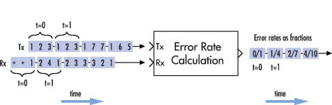
Рисунок ниже показывает, как блок сравнивает пары элементов и считает количество ошибочных событий. Tx и Rx входные параметры являются вектор-столбцами.
Этот пример предполагает, что шаг расчета каждого входного сигнала составляет 1 секунду и что параметры блока следующие:
-
Receive delay =
2 -
Computation delay =
0 -
Computation mode =
Entire frame
Оба входных сигнала являются вектор-столбцами длины три. Однако схематические расположения, каждый вектор-столбец горизонтально и выравнивает пары векторов, чтобы отразить задержку приема двух выборок. На каждом временном шаге блок сравнивает элементы Rx сигнал с теми из Tx сигнал, которые появляются непосредственно выше их в схематическом. Например, во время 1, блок выдерживает сравнение 2, 4, и 1 от Rx сигнал с 2, 3, и 1 от Tx сигнал.
Значения первых двух элементов Rx появитесь как звездочки, потому что они не влияют на выход. Точно так же 6 и 5 в Tx сигнал не влияет на выход до времени 3, хотя они влияли бы на выход во время 4.
В коэффициентах ошибок правой стороны рисунка каждый числитель во время t отражает количество ошибок при рассмотрении элементов Rx в течение времени t.
Подсчет ошибок целого кадра со сбросом
Если бы флажок Reset port блока был установлен, и сброс произошел во время = 3 секунды, то последний коэффициент ошибок будет 2/3 вместо 4/10. Это значение 2/3 отразило бы сравнение 3, 2, и 1 от Rx сигнал с 7, 7, и 1 от Tx сигнал. Рисунок ниже иллюстрирует этот сценарий. Tx и Rx входные параметры являются вектор-столбцами.

Подсчет ошибок на выборочных отсчетах в кадре
При использовании порта Sel, чтобы вычислить ошибки на задержанный сигнал, задержка должна быть добавлена к индексам Sel. Для получения дополнительной информации смотрите, Вычисляют, Ошибки для Задержанного Выбрали Samples.
Параметры
- Receive delay
-
Количество отсчетов, которым принятые данные отстают от передаваемых данных. (Если
TxилиRxвектор, затем каждая запись представляет выборку.) - Computation delay
-
Количество отсчетов, которые блок должен проигнорировать в начале сравнения.
- Computation mode
-
Любой
Entire frame,Select samples from mask, илиSelect samples from portВ зависимости от того, должен ли блок рассмотреть весь или только часть входных кадров. - Selected samples from frame
-
Вектор, который перечисляет индексы элементов
Rxструктурируйте вектор, который блок должен рассмотреть при создании сравнений. Это поле появляется, только если Computation mode установлен вSelect samples from mask. - Output data
-
Любой
WorkspaceилиPortВ зависимости от того, где вы хотите отправить выходные данные. - Variable name
-
Имя переменной для вектора выходных данных в основном рабочем пространстве MATLAB. Это поле появляется, только если Output data установлен в
Workspace. - Reset port
-
Если вы устанавливаете этот флажок, то дополнительный входной порт появляется, пометил
Rst. - Stop simulation
-
Если вы устанавливаете этот флажок, то симуляция запускается только, пока этот блок не обнаруживает конкретное количество ошибок или выполняет конкретное количество сравнений, какой бы ни на первом месте.
- Target number of errors
-
Остановки симуляции после обнаружения этого количества ошибок. Это поле активно, только если Stop simulation проверяется.
- Maximum number of symbols
-
Остановки симуляции после создания этого количества сравнений. Это поле активно, только если Stop simulation проверяется.
Поддерживаемые типы данных
| Порт | Поддерживаемые типы данных |
|---|---|
|
Tx |
|
|
Rx |
|
|
Sel |
|
|
Сброс |
|
Расширенные возможности
Генерация кода C/C++
Генерация кода C и C++ с помощью Simulink® Coder™.
Генерация HDL-кода
Сгенерируйте Verilog и код VHDL для FPGA и проекты ASIC с помощью HDL Coder™.
Этот блок может использоваться для видимости симуляции в подсистемах, которые генерируют HDL-код, но не включен в аппаратную реализацию.
Представлено до R2006a
This topic describes how to compute error statistics for various communications
systems.
Computation of Theoretical Error Statistics
The biterr function, discussed in the
Compute SERs and BERs Using Simulated Data section, can help you gather empirical error
statistics, but validating your results by comparing them to the theoretical error
statistics is good practice. For certain types of communications systems,
closed-form expressions exist for the computation of the bit error rate (BER) or an
approximate bound on the BER. The functions listed in this table compute the
closed-form expressions for the BER or a bound on it for the specified types of
communications systems.
| Type of Communications System | Function |
|---|---|
| Uncoded AWGN channel | berawgn
|
| Uncoded Rayleigh and Rician fading channel | berfading
|
| Coded AWGN channel | bercoding |
| Uncoded AWGN channel with imperfect synchronization | bersync
|
The analytical expressions used in these functions are discussed in
Analytical Expressions Used in BER Analysis. The reference pages of these functions also list
references to one or more books containing the closed-form expressions implemented
by the function.
Theoretical Performance Results
-
Plot Theoretical Error Rates
-
Compare Theoretical and Empirical Error Rates
Plot Theoretical Error Rates
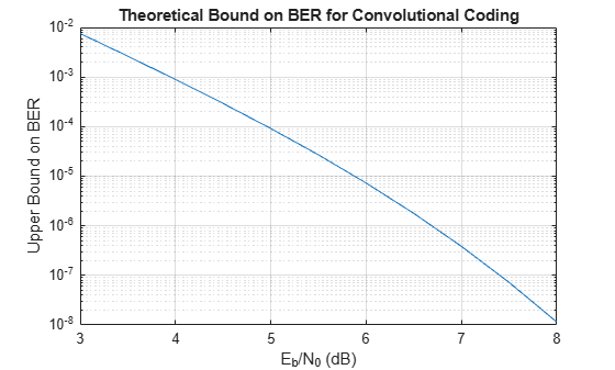
This example uses the bercoding function to compute upper bounds on BERs for convolutional coding with a soft-decision decoder.
coderate = 1/4; % Code rate
Create a structure, dspec, with information about the distance spectrum. Define the energy per bit to noise power spectral density ratio (Eb/N0) sweep range and generate the theoretical bound results.
dspec.dfree = 10; % Minimum free distance of code
dspec.weight = [1 0 4 0 12 0 32 0 80 0 192 0 448 0 1024 ...
    0 2304 0 5120 0]; % Distance spectrum of code
EbNo = 3:0.5:8;
berbound = bercoding(EbNo,'conv','soft',coderate,dspec);
Plot the theoretical bound results.
semilogy(EbNo,berbound)
xlabel('E_b/N_0 (dB)');
ylabel('Upper Bound on BER');
title('Theoretical Bound on BER for Convolutional Coding');
grid on;
Compare Theoretical and Empirical Error Rates
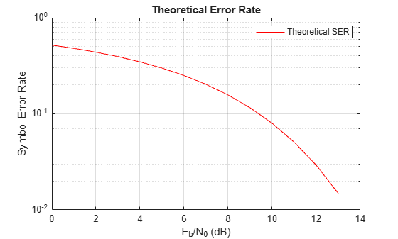
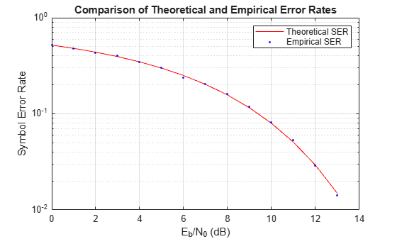
Using the berawgn function, compute the theoretical symbol error rates (SERs) for pulse amplitude modulation (PAM) over a range of Eb/N0 values. Simulate 8 PAM with an AWGN channel, and compute the empirical SERs. Compare the theoretical and then empirical SERs by plotting them on the same set of axes.
Compute and plot the theoretical SER using berawgn.
rng('default') % Set random number seed for repeatability
M = 8;
EbNo = 0:13;
[ber,ser] = berawgn(EbNo,'pam',M);

semilogy(EbNo,ser,'r');
legend('Theoretical SER');
title('Theoretical Error Rate');
xlabel('E_b/N_0 (dB)');
ylabel('Symbol Error Rate');
grid on;
Compute the empirical SER by simulating an 8 PAM communications system link. Define simulation parameters and preallocate variables needed for the results. As described in [1], because N0=2×(NVariance)2, add 3 dB to the Eb/N0 value when converting Eb/N0 values to SNR values.
n = 10000; % Number of symbols to process
k = log2(M); % Number of bits per symbol
snr = EbNo+3+10*log10(k); % In dB
ynoisy = zeros(n,length(snr));
z = zeros(n,length(snr));
errVec = zeros(3,length(EbNo));
Create an error rate calculator System object™ to compare decoded symbols to the original transmitted symbols.
errcalc = comm.ErrorRate;
Generate a random data message and apply PAM. Normalize the channel to the signal power. Loop the simulation to generate error rates over the range of SNR values.
x = randi([0 M-1],n,1); % Create message signal
y = pammod(x,M); % Modulate
signalpower = (real(y)'*real(y))/length(real(y));

for jj = 1:length(snr)
    reset(errcalc)
    ynoisy(:,jj) = awgn(real(y),snr(jj),'measured'); % Add AWGN
    z(:,jj) = pamdemod(complex(ynoisy(:,jj)),M); % Demodulate
    errVec(:,jj) = errcalc(x,z(:,jj)); % Compute SER from simulation
end
Compare the theoretical and empirical results.
hold on;
semilogy(EbNo,errVec(1,:),'b.');
legend('Theoretical SER','Empirical SER');
title('Comparison of Theoretical and Empirical Error Rates');
hold off;
Performance Results via Simulation
-
Section Overview
-
Compute SERs and BERs Using Simulated Data
Section Overview
This section describes how to compare the data messages that enter and leave
a communications system simulation and how to compute error statistics using the
Monte Carlo technique. Simulations can measure system performance by using the
data messages before transmission and after reception to compute the BER or SER
for a communications system. To explore physical layer components used to model
and simulate communications systems, see PHY Components.
Curve fitting can be useful when you have a small or imperfect data set but
want to plot a smooth curve for presentation purposes. To explore the use of
curve fitting when computing performance results via simulation, see the Curve Fitting for Error Rate Plots section.
Compute SERs and BERs Using Simulated Data
The example shows how to compute SERs and BERs using the biterr and symerr functions, respectively. The symerr function compares two sets of data and computes the number of symbol errors and the SER. The biterr function compares two sets of data and computes the number of bit errors and the BER. An error is a discrepancy between corresponding points in the two sets of data.
The two sets of data typically represent messages entering a transmitter and recovered messages leaving a receiver. You can also compare data entering and leaving other parts of your communications system (for example, data entering an encoder and data leaving a decoder).
If your communications system uses several bits to represent one symbol, counting symbol errors is different from counting bit errors. In either the symbol- or bit-counting case, the error rate is the number of errors divided by the total number of transmitted symbols or bits, respectively.
Typically, simulating enough data to produce at least 100 errors provides accurate error rate results. If the error rate is very small (for example, 10-6 or less), using the semianalytic technique might compute the result more quickly than using a simulation-only approach. For more information, see the Performance Results via Semianalytic Technique section.
Compute Error Rates
Use the symerr function to compute the SERs for a noisy linear block code. Apply no digital modulation, so that each symbol contains a single bit. When each symbol is a single bit, the symbol errors and bit errors are the same.
After artificially adding noise to the encoded message, compare the resulting noisy code to the original code. Then, decode and compare the decoded message to the original message.
m = 3; % Set parameters for Hamming code
n = 2^m-1;
k = n-m;
msg = randi([0 1],k*200,1); % Specify 200 messages of k bits each
code = encode(msg,n,k,'hamming');
codenoisy = bsc(code,0.95); % Add noise
newmsg = decode(codenoisy,n,k,'hamming'); % Decode and correct errors
Compute the SERs.
[~,noisyVec] = symerr(code,codenoisy);
[~,decodedVec] = symerr(msg,newmsg);
The error rate decreases after decoding because the Hamming decoder correct errors based on the error-correcting capability of the decoder configuration. Because random number generators produce the message and noise is added, results vary from run to run. Display the SERs.
disp(['SER in the received code: ',num2str(noisyVec(1))])
SER in the received code: 0.94571
disp(['SER after decoding: ',num2str(decodedVec(1))])
SER after decoding: 0.9675
Comparing SER and BER
These commands show the difference between symbol errors and bit errors in various situations.
Create two three-element decimal vectors and show the binary representation. The vector a contains three 2-bit symbols, and the vector b contains three 3-bit symbols.
bpi = 3; % Bits per integer
a = [1 2 3];
b = [1 4 4];
int2bit(a,bpi)
ans = 3×3

     0     0     0
     0     1     1
     1     0     1
ans = 3×3

     0     1     1
     0     0     0
     1     0     0
Compare the binary values of the two vectors and compute the number of errors and the error rate by using the biterr and symerr functions.
format rat % Display fractions instead of decimals
[snum,srate] = symerr(a,b)
snum is 2 because the second and third entries have bit differences. srate is 2/3 because the total number of symbols is 3.
[bnum,brate] = biterr(a,b)
bnum is 5 because the second entries differ in two bits, and the third entries differ in three bits. brate is 5/9 because the total number of bits is 9. By definition, the total number of bits is the number of entries in a for symbol error computations or b for bit error computations times the maximum number of bits among all entries of a and b, respectively.
Performance Results via Semianalytic Technique
The technique described in the Performance Results via Simulation
section can work for a large variety of communications systems but can be
prohibitively time-consuming for small error rates (for example,
10-6 or less). The semianalytic technique is an
alternative way to compute error rates. The semianalytic technique can produce
results faster than a nonanalytic method that uses simulated data.
For more information on implementing the semianalytic technique using a
combination of simulation and analysis to determine the error rate of a
communications system, see the semianalytic function.
Error Rate Plots
-
Section Overview
-
Creation of Error Rate Plots Using
semilogy
Function -
Curve Fitting for Error Rate Plots
-
Use Curve Fitting on Error Rate Plot
Section Overview
Error rate plots can be useful when examining the performance of a
communications system and are often included in publications. This section
discusses and demonstrates tools you can use to create error rate plots, modify
them to suit your needs, and perform curve fitting on the error rate data and
the plots.
Creation of Error Rate Plots Using semilogy Function
In many error rate plots, the horizontal axis indicates
Eb/N0
values in dB, and the vertical axis indicates the error rate using a logarithmic
(base 10) scale. For examples that create such a plot using the semilogy function, see Compare Theoretical and Empirical Error Rates and Plot Theoretical Error Rates.
Curve Fitting for Error Rate Plots
Curve fitting can be useful when you have a small or imperfect data set but
want to plot a smooth curve for presentation purposes. The berfit function includes
curve-fitting capabilities that help your analysis when the empirical data
describes error rates at different
Eb/N0
values. This function enables you to:
-
Customize various relevant aspects of the curve-fitting process, such
as a list of selections for the type of closed-form function used to
generate the fit. -
Plot empirical data along with a curve that
berfitfits to the
data. -
Interpolate points on the fitted curve between
Eb/N0
values in your empirical data set to smooth the plot. -
Collect relevant information about the fit, such as the numerical
values of points along the fitted curve and the coefficients of the fit
expression.
Note
The berfit function is
intended for curve fitting or interpolation, not extrapolation.
Extrapolating BER data beyond an order of magnitude below the smallest
empirical BER value is inherently unreliable.
Use Curve Fitting on Error Rate Plot
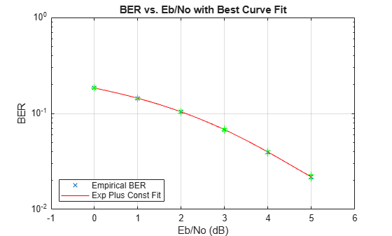
This example simulates a simple differential binary phase shift keying (DBPSK) communications system and plots error rate data for a series of Eb/N0 values. It uses the berfit and berconfint functions to fit a curve to a set of empirical error rates.
Initialize Simulation Parameters
Specify the input signal message length, modulation order, range of Eb/N0 values to simulate, and the minimum number of errors that must occur before the simulation computes an error rate for a given Eb/N0 value. Preallocate variables for final results and interim results.
Typically, for statistically accurate error rate results, the minimum number of errors must be on the order of 100. This simulation uses a small number of errors to shorten the run time and to illustrate how curve fitting can smooth a set of results.
siglen = 100000; % Number of bits in each trial
M = 2; % DBPSK is binary
EbN0vec = 0:5; % Vector of EbN0 values
minnumerr = 5; % Compute BER after only 5 errors occur
numEbN0 = length(EbN0vec); % Number of EbN0 values

ber = zeros(1,numEbN0); % Final BER values
berVec = zeros(3,numEbN0); % Updated BER values
intv = cell(1,numEbN0); % Cell array of confidence intervals
Create an error rate calculator System object™.
errorCalc = comm.ErrorRate;
Loop the Simulation
Simulate the DBPSK-modulated communications system and compute the BER using a for loop to vary the Eb/N0 value. The inner while loop ensures that a minimum number of bit errors occur for each Eb/N0 value. Error rate statistics are saved for each Eb/N0 value and used later in this example when curve fitting and plotting.
for jj = 1:numEbN0
    EbN0 = EbN0vec(jj);
    snr = EbN0; % For binary modulation SNR = EbN0
    reset(errorCalc)

    while (berVec(2,jj) < minnumerr)
        msg = randi([0,M-1],siglen,1); % Generate message sequence
        txsig = dpskmod(msg,M); % Modulate
        rxsig = awgn(txsig,snr,'measured'); % Add noise
        decodmsg = dpskdemod(rxsig,M); % Demodulate
        berVec(:,jj) = errorCalc(msg,decodmsg); % Calculate BER
    end
Use the berconfint function to compute the error rate at a 98% confidence interval for the Eb/N0 values.
    [ber(jj),intv1] = berconfint(berVec(2,jj),berVec(3,jj),0.98);
    intv{jj} = intv1;
    disp(['EbN0 = ' num2str(EbN0) ' dB, ' num2str(berVec(2,jj)) ...
        ' errors, BER = ' num2str(ber(jj))])
end
EbN0 = 0 dB, 18392 errors, BER = 0.18392
EbN0 = 1 dB, 14307 errors, BER = 0.14307
EbN0 = 2 dB, 10190 errors, BER = 0.1019
EbN0 = 3 dB, 6940 errors, BER = 0.0694
EbN0 = 4 dB, 4151 errors, BER = 0.04151
EbN0 = 5 dB, 2098 errors, BER = 0.02098
Use the berfit function to plot the best fitted curve, interpolating between BER points to get a smooth plot. Add confidence intervals to the plot.
fitEbN0 = EbN0vec(1):0.25:EbN0vec(end); % Interpolation values
berfit(EbN0vec,ber,fitEbN0);
hold on;
for jj=1:numEbN0
    semilogy([EbN0vec(jj) EbN0vec(jj)],intv{jj},'g-+');
end
hold off;
See Also
Apps
- Bit Error Rate Analysis
Functions
berawgn|bercoding|berconfint|berfading|berfit|bersync
Related Topics
- Analyze Performance with Bit Error Rate Analysis App
- Analytical Expressions Used in BER Analysis
This is machine translation
Translated by ![]()
Mouseover text to see original. Click the button below to return to the English version of the page.
Note: This page has been translated by MathWorks. Click here to see
To view all translated materials including this page, select Country from the country navigator on the bottom of this page.
Theoretical Results
Common Notation
The following notation is used throughout this Appendix:
| Quantity or Operation | Notation |
|---|---|
| Size of modulation constellation |
M |
| Number of bits per symbol |
k=log2M |
| Energy per bit-to-noise power-spectral-density ratio |
EbN0 |
| Energy per symbol-to-noise power-spectral-density ratio |
EsN0=kEbN0 |
| Bit error rate (BER) |
Pb |
| Symbol error rate (SER) |
Ps |
| Real part |
Re[⋅] |
| Largest integer smaller than |
⌊⋅⌋ |
The following mathematical functions are used:
| Function | Mathematical Expression |
|---|---|
| Q function |
Q(x)=12π∫x∞exp(−t2/2)dt |
| Marcum Q function |
Q(a,b)=∫b∞texp(−t2+a22)I0(at)dt |
| Modified Bessel function of the first kind of order ν |
Iν(z)=∑k=0∞(z/2)υ+2kk!Γ(ν+k+1) where Γ(x)=∫0∞e−ttx−1dt is the gamma function. |
| Confluent hypergeometric function |
F11(a,c;x)=∑k=0∞(a)k(c)kxkk! where the Pochhammer symbol, (λ)k, is defined as (λ)0=1, (λ)k=λ(λ+1)(λ+2)⋯(λ+k−1). |
The following acronyms are used:
| Acronym | Definition |
|---|---|
| M-PSK | M-ary phase-shift keying |
| DE-M-PSK | Differentially encoded M-ary phase-shift keying |
| BPSK | Binary phase-shift keying |
| DE-BPSK | Differentially encoded binary phase-shift keying |
| QPSK | Quaternary phase-shift keying |
| DE-QPSK | Differentially encoded quadrature phase-shift keying |
| OQPSK | Offset quadrature phase-shift keying |
| DE-OQPSK | Differentially encoded offset quadrature phase-shift keying |
| M-DPSK | M-ary differential phase-shift keying |
| M-PAM | M-ary pulse amplitude modulation |
| M-QAM | M-ary quadrature amplitude modulation |
| M-FSK | M-ary frequency-shift keying |
| MSK | Minimum shift keying |
| M-CPFSK | M-ary continuous-phase frequency-shift keying |
Analytical Expressions Used in berawgn
-
M-PSK
-
DE-M-PSK
-
OQPSK
-
DE-OQPSK
-
M-DPSK
-
M-PAM
-
M-QAM
-
Orthogonal M-FSK with Coherent Detection
-
Nonorthogonal 2-FSK with Coherent Detection
-
Orthogonal M-FSK with Noncoherent Detection
-
Nonorthogonal 2-FSK with Noncoherent Detection
-
Precoded MSK with Coherent Detection
-
Differentially Encoded MSK with Coherent Detection
-
MSK with Noncoherent Detection (Optimum Block-by-Block)
-
CPFSK Coherent Detection (Optimum Block-by-Block)
M-PSK. From equation 8.22 in [2]
The following expression is very close, but not strictly equal,
to the exact BER (from [4] and equation 8.29 from [2]):
where wi’=wi+wM−i, wM/2’=wM/2, wiis the Hamming weight of bits
assigned to symbol i, and
Special case of M=2, e.g., BPSK (equation
5.2-57 from [1]):
Special case of M=4, e.g., QPSK (equations
5.2-59 and 5.2-62 from [1]):
DE-M-PSK. M=2, e.g., DE-BPSK (equation 8.36
from [2]):
M=4, e.g., DE-QPSK (equation 8.38
from [2]):
From equation 5 in [3]:
OQPSK. Same BER/SER as QPSK [2].
DE-OQPSK. Same BER/SER as DE-QPSK [3].
M-DPSK. From equation 8.84 in [2]:
The following expression is very close, but not strictly equal,
to the exact BER [4]:
where wi’=wi+wM−i, wM/2’=wM/2, wi is the Hamming weight of bits
assigned to symbol i, and
Special case of M=2 (equation 8.85
from [2]):
M-PAM. From equations 8.3 and 8.7 in [2], and
equation 5.2-46 in [1]:
From [5]:
M-QAM. For square M-QAM, k=log2M is even (equation
8.10 from [2], and
equations 5.2-78 and 5.2-79 from [1]):
From [5]:
For rectangular (non-square) M-QAM, k=log2M is odd, M=I×J, I=2k−12, and J=2k+12:
From [5]:
where
and
Orthogonal M-FSK with Coherent Detection. From equation 8.40 in [2] and
equation 5.2-21 in [1]:
Nonorthogonal 2-FSK with Coherent Detection. For M=2 (from equation 5.2-21 in [1] and equation 8.44 in [2]):
ρis the complex correlation coefficient:
where s˜1(t) and s˜2(t) are complex lowpass signals,
and
For example:
where Δf=f1−f2.
(from equation 8.44 in [2], where h=ΔfTb)
Orthogonal M-FSK with Noncoherent Detection. From equation 5.4-46 in [1] and equation 8.66 in [2]:
Nonorthogonal 2-FSK with Noncoherent Detection. For M=2 (from equation 5.4-53 in [1] and equation 8.69 in [2]):
where
Precoded MSK with Coherent Detection. Same BER/SER as BPSK.
Differentially Encoded MSK with Coherent Detection. Same BER/SER as DE-BPSK.
MSK with Noncoherent Detection (Optimum Block-by-Block). Upper bound (from equations 10.166 and 10.164 in [6]):
where
CPFSK Coherent Detection (Optimum Block-by-Block). Lower bound (from equation 5.3-17 in [1]):
Upper bound:
where h is the modulation index, and Kδmin is the number of paths having
the minimum distance.
Analytical Expressions Used in berfading
-
Notation
-
M-PSK with MRC
-
DE-M-PSK with MRC
-
M-PAM with MRC
-
M-QAM with MRC
-
M-DPSK with Postdetection EGC
-
Orthogonal 2-FSK, Coherent Detection with MRC
-
Nonorthogonal 2-FSK, Coherent Detection with MRC
-
Orthogonal M-FSK, Noncoherent Detection with EGC
-
Nonorthogonal 2-FSK, Noncoherent Detection with No Diversity
Notation. The following notation is used for the expressions found in berfading.
| Value | Notation |
|---|---|
| Power of the fading amplitude r | Ω=E[r2], where E[⋅] denotes statistical expectation |
| Number of diversity branches |
L |
| SNR per symbol per branch |
γ¯l=(ΩlEsN0)/L=(ΩlkEbN0)/L For identically-distributed diversity γ¯=(ΩkEbN0)/L |
| Moment generating functions for each diversity branch |
Rayleigh fading: Mγl(s)=11−sγ¯l Rician fading: Mγl(s)=1+K1+K−sγ¯le[Ksγ¯l(1+K)−sγ¯l] where K is the ratio of For |
The following acronyms are used:
| Acronym | Definition |
|---|---|
| MRC | maximal-ratio combining |
| EGC | equal-gain combining |
M-PSK with MRC. From equation 9.15 in [2]:
From [4] and [2]:
where wi’=wi+wM−i, wM/2’=wM/2, wi is the Hamming weight of bits
assigned to symbol i, and
For the special case of Rayleigh fading with M=2 (from equations C-18, C-21,
and Table C-1 in [6]):
where
If L=1:
DE-M-PSK with MRC. For M=2 (from equations 8.37 and 9.8-9.11
in [2]):
M-PAM with MRC. From equation 9.19 in [2]:
From [5] and [2]:
M-QAM with MRC. For square M-QAM, k=log2M is even (equation
9.21 in [2]):
From [5] and [2]:
For rectangular (nonsquare) M-QAM, k=log2M is odd, M=I×J, I=2k−12, J=2k+12, γ¯l=Ωllog2(IJ)EbN0, and
From [5] and [2]:
M-DPSK with Postdetection EGC. From equation 8.165 in [2]:
From [4] and [2]:
where wi’=wi+wM−i, wM/2’=wM/2, wi is the Hamming weight of bits
assigned to symbol i, and
For the special case of Rayleigh fading with M=2, and L=1 (equation 8.173 from [2]):
Orthogonal 2-FSK, Coherent Detection with MRC. From equation 9.11 in [2]:
For the special case of Rayleigh fading (equations 14.4-15 and
14.4-21 in [1]):
Nonorthogonal 2-FSK, Coherent Detection with MRC. Equations 9.11 and 8.44 in [2]:
For the special case of Rayleigh fading with L=1 (equation 20 in [8] and equation 8.130 in [2]):
Orthogonal M-FSK, Noncoherent Detection with EGC. Rayleigh fading (equation 14.4-47 in [1]):
Rician fading (equation 41 in [8]):
where
and I[a,b](i)=1 if a≤i≤b and 0 otherwise.
Nonorthogonal 2-FSK, Noncoherent Detection with No Diversity. From equation 8.163 in [2]:
where
Analytical Expressions Used in bercoding and BERTool
-
Common Notation for This Section
-
Block Coding
-
Convolutional Coding
Common Notation for This Section
| Description | Notation |
|---|---|
| Energy-per-information bit-to-noise power-spectral-density ratio |
γb=EbN0 |
| Message length |
K |
| Code length |
N |
| Code rate |
Rc=KN |
Block Coding. Specific notation for block coding expressions: dmin is the minimum distance of the
code.
Soft Decision
BPSK, QPSK, OQPSK, PAM-2, QAM-4, and precoded MSK (equation 8.1-52 in
[1]):
DE-BPSK, DE-QPSK, DE-OQPSK, and DE-MSK:
BFSK, coherent detection (equations 8.1-50 and 8.1-58 in [1]):
BFSK, noncoherent square-law detection (equations 8.1-65 and 8.1-64 in
[1]):
DPSK:
Hard Decision
General linear block code (equations 4.3, 4.4 in [9], and 12.136 in [6]):
Hamming code (equations 4.11, 4.12 in [9], and 6.72, 6.73 in [7]):
(24, 12) extended Golay code (equation 4.17 in [9], and 12.139 in [6]):
where βm is the average number of channel symbol errors that remain
in corrected N-tuple when the channel caused
m symbol errors (table 4.2 in [9]).
Reed-Solomon code with N=Q−1=2q−1:
for FSK (equations 4.25, 4.27 in [9], 8.1-115, 8.1-116 in [1], 8.7, 8.8 in [7], and 12.142, 12.143 in [6]), and
otherwise.
If log2Q/log2M=q/k=h where h is an integer (equation 1 in
[10]):
where s is the symbol error rate (SER) in an uncoded
AWGN channel.
For example, for BPSK, M=2 and Ps=1−(1−s)q
Otherwise, Ps is given by table 1 and equation 2 in [10].
Convolutional Coding. Specific notation for convolutional coding expressions: dfree is the free distance of the
code, and ad is the number of paths of distance d from
the all-zero path that merge with the all-zero path for the first
time.
Soft Decision
From equations 8.2-26, 8.2-24, and 8.2-25 in [1], and equations 13.28 and 13.27 in [6]:
with transfer function
where f(d) is the exponent of N as a function of
d.
Results for BPSK, QPSK, OQPSK, PAM-2, QAM-4, precoded MSK, DE-BPSK,
DE-QPSK, DE-OQPSK, DE-MSK, DPSK, and BFSK are obtained as:
where Pb is the BER in the corresponding uncoded AWGN channel. For
example, for BPSK (equation 8.2-20 in [1]):
Hard Decision
From equations 8.2-33, 8.2-28, and 8.2-29 in [1], and equations 13.28, 13.24, and 13.25 in [6]:
where
when d is odd, and
when d is even (p is the bit error
rate (BER) in an uncoded AWGN channel).
Performance Results via Simulation
-
Section Overview
-
Using Simulated Data to Compute Bit and Symbol Error Rates
-
Example: Computing Error Rates
-
Comparing Symbol Error Rate and Bit Error Rate
Section Overview
One way to compute the bit error rate or symbol error rate for a communication system is to
simulate the transmission of data messages and compare all messages before and
after transmission. The simulation of the communication system components using
Communications Toolbox™ is covered in other parts of this guide. This section describes
how to compare the data messages that enter and leave the simulation.
Another example of computing performance results via simulation
is in Curve Fitting for Error Rate Plots in the discussion of curve
fitting.
Using Simulated Data to Compute Bit and Symbol Error Rates
The biterr function compares two sets of
data and computes the number of bit errors and the bit error rate.
The symerr function compares two sets of data
and computes the number of symbol errors and the symbol error rate.
An error is a discrepancy between corresponding points in the two
sets of data.
Of the two sets of data, typically one represents messages entering
a transmitter and the other represents recovered messages leaving
a receiver. You might also compare data entering and leaving other
parts of your communication system, for example, data entering an
encoder and data leaving a decoder.
If your communication system uses several bits to represent
one symbol, counting bit errors is different from counting symbol
errors. In either the bit- or symbol-counting case, the error rate
is the number of errors divided by the total number (of bits or symbols)
transmitted.
Note
To ensure an accurate error rate, you should typically simulate
enough data to produce at least 100 errors.
If the error rate is very small (for example, 10-6 or
smaller), the semianalytic technique might compute the result more
quickly than a simulation-only approach. See Performance Results via the Semianalytic Technique for more
information on how to use this technique.
Example: Computing Error Rates
The script below uses the symerr function
to compute the symbol error rates for a noisy linear block code. After
artificially adding noise to the encoded message, it compares the
resulting noisy code to the original code. Then it decodes and compares
the decoded message to the original one.
m = 3; n = 2^m-1; k = n-m; % Prepare to use Hamming code.
msg = randi([0 1],k*200,1); % 200 messages of k bits each
code = encode(msg,n,k,'hamming');
codenoisy = rem(code+(rand(n*200,1)>.95),2); % Add noise.
% Decode and correct some errors.
newmsg = decode(codenoisy,n,k,'hamming');
% Compute and display symbol error rates.
noisyVec = step(comm.ErrorRate,code,codenoisy);
decodedVec = step(comm.ErrorRate,msg,newmsg);
disp(['Error rate in the received code: ',num2str(noisyVec(1))])
disp(['Error rate after decoding: ',num2str(decodedVec(1))])
The output is below. The error rate decreases after decoding
because the Hamming decoder corrects some of the errors. Your results
might vary because this example uses random numbers.
Error rate in the received code: 0.054286
Error rate after decoding: 0.03
Comparing Symbol Error Rate and Bit Error Rate
In the example above, the symbol errors and bit errors are the
same because each symbol is a bit. The commands below illustrate the
difference between symbol errors and bit errors in other situations.
a = [1 2 3]'; b = [1 4 4]';
format rat % Display fractions instead of decimals.
% Create ErrorRate Calculator System object
serVec = step(comm.ErrorRate,a,b);
srate = serVec(1)
snum = serVec(2)
% Convert integers to bits
hIntToBit = comm.IntegerToBit(3);
a_bit = step(hIntToBit, a);
b_bit = step(hIntToBit, b);
% Calculate BER
berVec = step(comm.ErrorRate,a_bit,b_bit);
brate = berVec(1)
bnum = berVec(2)
The output is below.
snum =

      2


srate =

     2/3


bnum =

      5


brate =

     5/9
bnum is 5 because the second entries differ
in two bits and the third entries differ in three bits. brate is
5/9 because the total number of bits is 9. The total number of bits
is, by definition, the number of entries in a or b times
the maximum number of bits among all entries of a and b.
Performance Results via the Semianalytic Technique
The technique described in Performance Results via Simulation works well for a large
variety of communication systems, but can be prohibitively time-consuming
if the system’s error rate is very small (for example, 10-6 or
smaller). This section describes how to use the semianalytic technique
as an alternative way to compute error rates. For certain types of
systems, the semianalytic technique can produce results much more
quickly than a nonanalytic method that uses only simulated data.
The semianalytic technique uses a combination of simulation
and analysis to determine the error rate of a communication system.
The semianalytic function in Communications Toolbox helps
you implement the semianalytic technique by performing some of the
analysis.
When to Use the Semianalytic Technique
The semianalytic technique works well for certain types of communication
systems, but not for others. The semianalytic technique is applicable
if a system has all of these characteristics:
-
Any effects of multipath fading, quantization, and
amplifier nonlinearities must precede the effects
of noise in the actual channel being modeled. -
The receiver is perfectly synchronized with the carrier,
and timing jitter is negligible. Because phase noise and timing jitter
are slow processes, they reduce the applicability of the semianalytic
technique to a communication system. -
The noiseless simulation has no errors in the received
signal constellation. Distortions from sources other than noise should
be mild enough to keep each signal point in its correct decision region.
If this is not the case, the calculated BER is too low. For instance,
if the modeled system has a phase rotation that places the received
signal points outside their proper decision regions, the semianalytic
technique is not suitable to predict system performance.
Furthermore, the semianalytic function
assumes that the noise in the actual channel being modeled is Gaussian.
For details on how to adapt the semianalytic technique for non-Gaussian
noise, see the discussion of generalized exponential distributions
in [11].
Procedure for the Semianalytic Technique
The procedure below describes how you would typically implement
the semianalytic technique using the semianalytic function:
-
Generate a message signal containing at least ML symbols,
where M is the alphabet size of the modulation and L is the length
of the impulse response of the channel in symbols. A common approach
is to start with an augmented binary pseudonoise (PN) sequence of
total length(log2M)ML.
An augmented PN sequence is a PN sequence with
an extra zero appended, which makes the distribution of ones and zeros
equal. -
Modulate a carrier with the message signal using baseband modulation.
Supported modulation types are listed on the reference page forsemianalytic.
Shape the resultant signal with rectangular pulse shaping, using
the oversampling factor that you will later use to filter the modulated
signal. Store the result of this step astxsigfor
later use. -
Filter the modulated signal with a transmit filter. This filter
is often a square-root raised cosine filter, but you can also use
a Butterworth, Bessel, Chebyshev type 1 or 2, elliptic, or more general
FIR or IIR filter. If you use a square-root raised cosine filter,
use it on the nonoversampled modulated signal and specify the oversampling
factor in the filtering function. If you use another filter type,
you can apply it to the rectangularly pulse shaped signal. -
Run the filtered signal through a noiseless channel.
This channel can include multipath fading effects, phase shifts,
amplifier nonlinearities, quantization, and additional filtering,
but it must not include noise. Store the result of this step asrxsigfor
later use. -
Invoke the
semianalyticfunction
using thetxsigandrxsigdata
from earlier steps. Specify a receive filter as a pair of input arguments,
unless you want to use the function’s default filter. The function
filtersrxsigand then determines the error probability
of each received signal point by analytically applying the Gaussian
noise distribution to each point. The function averages the error
probabilities over the entire received signal to determine the overall
error probability. If the error probability calculated in this way
is a symbol error probability, the function converts it to a bit error
rate, typically by assuming Gray coding. The function returns the
bit error rate (or, in the case of DQPSK modulation, an upper bound
on the bit error rate).
Example: Using the Semianalytic Technique
The example below illustrates the procedure described above,
using 16-QAM modulation. It also compares the error rates obtained
from the semianalytic technique with the theoretical error rates obtained
from published formulas and computed using the berawgn function.
The resulting plot shows that the error rates obtained using the two
methods are nearly identical. The discrepancies between the theoretical
and computed error rates are largely due to the phase offset in this
example’s channel model.
% Step 1. Generate message signal of length >= M^L.
M = 16; % Alphabet size of modulation
L = 1; % Length of impulse response of channel
msg = [0:M-1 0]; % M-ary message sequence of length > M^L

% Step 2. Modulate the message signal using baseband modulation.
%hMod = comm.RectangularQAMModulator(M);  % Use 16-QAM.
%modsig = step(hMod,msg'); % Modulate data
modsig = qammod(msg',M); % Modulate data
Nsamp = 16;
modsig = rectpulse(modsig,Nsamp); % Use rectangular pulse shaping.

% Step 3. Apply a transmit filter.
txsig = modsig; % No filter in this example

% Step 4. Run txsig through a noiseless channel.
rxsig = txsig*exp(1i*pi/180); % Static phase offset of 1 degree
% Step 5. Use the semianalytic function.
% Specify the receive filter as a pair of input arguments.
% In this case, num and den describe an ideal integrator.
num = ones(Nsamp,1)/Nsamp;
den = 1;
EbNo = 0:20; % Range of Eb/No values under study
ber = semianalytic(txsig,rxsig,'qam',M,Nsamp,num,den,EbNo);

% For comparison, calculate theoretical BER.
bertheory = berawgn(EbNo,'qam',M);

% Plot computed BER and theoretical BER.
figure; semilogy(EbNo,ber,'k*');
hold on; semilogy(EbNo,bertheory,'ro');
title('Semianalytic BER Compared with Theoretical BER');
legend('Semianalytic BER with Phase Offset',...
   'Theoretical BER Without Phase Offset','Location','SouthWest');
hold off;
This example creates a figure like the one below.

Theoretical Performance Results
-
Computing Theoretical Error Statistics
-
Plotting Theoretical Error Rates
-
Comparing Theoretical and Empirical Error Rates
Computing Theoretical Error Statistics
While the biterr function discussed above
can help you gather empirical error statistics, you might also compare
those results to theoretical error statistics. Certain types of communication
systems are associated with closed-form expressions for the bit error
rate or a bound on it. The functions listed in the table below compute
the closed-form expressions for some types of communication systems,
where such expressions exist.
| Type of Communication System | Function |
|---|---|
| Uncoded AWGN channel | berawgn |
| Coded AWGN channel | bercoding |
| Uncoded Rayleigh and Rician fading channel | berfading |
| Uncoded AWGN channel with imperfect synchronization | bersync |
Each function’s reference page lists one or more books containing
the closed-form expressions that the function implements.
Plotting Theoretical Error Rates
The example below uses the bercoding function
to compute upper bounds on bit error rates for convolutional coding
with a soft-decision decoder. The data used for the generator and
distance spectrum are from [1] and [12], respectively.
coderate = 1/4; % Code rate
% Create a structure dspec with information about distance spectrum.
dspec.dfree = 10; % Minimum free distance of code
dspec.weight = [1 0 4 0 12 0 32 0 80 0 192 0 448 0 1024 ...
   0 2304 0 5120 0]; % Distance spectrum of code
EbNo = 3:0.5:8;
berbound = bercoding(EbNo,'conv','soft',coderate,dspec);
semilogy(EbNo,berbound) % Plot the results.
xlabel('E_b/N_0 (dB)'); ylabel('Upper Bound on BER');
title('Theoretical Bound on BER for Convolutional Coding');
grid on;
This example produces the following plot.

Comparing Theoretical and Empirical Error Rates
The example below uses the berawgn function
to compute symbol error rates for pulse amplitude modulation (PAM)
with a series of Eb/N0 values. For comparison, the code simulates
8-PAM with an AWGN channel and computes empirical symbol error rates.
The code also plots the theoretical and empirical symbol error rates
on the same set of axes.
% 1. Compute theoretical error rate using BERAWGN.
rng('default')      % Set random number seed for repeatability
%
M = 8; EbNo = 0:13;
[ber, ser] = berawgn(EbNo,'pam',M);
% Plot theoretical results.
figure; semilogy(EbNo,ser,'r');
xlabel('E_b/N_0 (dB)'); ylabel('Symbol Error Rate');
grid on; drawnow;

% 2. Compute empirical error rate by simulating.
% Set up.
n = 10000; % Number of symbols to process
k = log2(M); % Number of bits per symbol
% Convert from EbNo to SNR.
% Note: Because No = 2*noiseVariance^2, we must add 3 dB
% to get SNR. For details, see Proakis' book listed in
% "Selected Bibliography for Performance Evaluation."
snr = EbNo+3+10*log10(k);
% Preallocate variables to save time.
ynoisy = zeros(n,length(snr));
z      = zeros(n,length(snr));
berVec = zeros(3,length(EbNo));

% PAM modulation and demodulation system objects
%h  = comm.PAMModulator(M);
%h2 = comm.PAMDemodulator(M);

% AWGNChannel System object
hChan = comm.AWGNChannel('NoiseMethod', 'Signal to noise ratio (SNR)');


% ErrorRate calculator System object to compare decoded symbols to the
% original transmitted symbols.
hErrorCalc = comm.ErrorRate;

% Main steps in the simulation
x = randi([0 M-1],n,1); % Create message signal.
%y = step(h,x); % Modulate.
y = pammod(x,M); % Modulate.
hChan.SignalPower = (real(y)' * real(y))/ length(real(y));

% Loop over different SNR values.
for jj = 1:length(snr)
    reset(hErrorCalc)
    hChan.SNR = snr(jj); % Assign Channel SNR
    ynoisy(:,jj) = step(hChan,real(y)); % Add AWGN
%    z(:,jj) = step(h2,complex(ynoisy(:,jj))); % Demodulate.
    z(:,jj) = pamdemod(complex(ynoisy(:,jj)),M); % Demodulate.

    % Compute symbol error rate from simulation.
    berVec(:,jj) = step(hErrorCalc, x, z(:,jj));
end

% 3. Plot empirical results, in same figure.
hold on; semilogy(EbNo,berVec(1,:),'b.');
legend('Theoretical SER','Empirical SER');
title('Comparing Theoretical and Empirical Error Rates');
hold off;
This example produces a plot like the one in the following figure.
Your plot might vary because the simulation uses random numbers.

Error Rate Plots
-
Section Overview
-
Creating Error Rate Plots Using
semilogy -
Curve Fitting for Error Rate Plots
-
Example: Curve Fitting for an Error Rate Plot
Section Overview
Error rate plots provide a visual way to examine the performance
of a communication system, and they are often included in publications.
This section mentions some of the tools you can use to create error
rate plots, modify them to suit your needs, and do curve
fitting on error rate data. It also provides an example of curve
fitting. For more detailed discussions about the more general
plotting capabilities in MATLAB®, see the MATLAB documentation
set.
Creating Error Rate Plots Using semilogy
In many error rate plots, the horizontal axis indicates Eb/N0 values
in dB and the vertical axis indicates the error rate using a logarithmic
(base 10) scale. To see an example of such a plot, as well as the
code that creates it, see Comparing Theoretical and Empirical Error Rates. The part
of that example that creates the plot uses the semilogy function
to produce a logarithmic scale on the vertical axis and a linear scale
on the horizontal axis.
Other examples that illustrate the use of semilogy are
in these sections:
-
Example: Using the Semianalytic Technique, which also illustrates
-
Plotting two sets of data on one pair of axes
-
Adding a title
-
Adding a legend
-
-
Plotting Theoretical Error Rates, which also illustrates
-
Adding axis labels
-
Adding grid lines
-
Curve Fitting for Error Rate Plots
Curve fitting is useful when you have a small or imperfect data set but want to plot a smooth
curve for presentation purposes. The berfit function in
Communications Toolbox offers curve-fitting capabilities that are well suited to the
situation when the empirical data describes error rates at different
Eb/N0 values. This function
enables you to
-
Customize various relevant aspects of the curve-fitting
process, such as the type of closed-form function (from a list of
preset choices) used to generate the fit. -
Plot empirical data along with a curve that
berfitfits
to the data. -
Interpolate points on the fitted curve between Eb/N0 values
in your empirical data set to make the plot smoother looking. -
Collect relevant information about the fit, such as
the numerical values of points along the fitted curve and the coefficients
of the fit expression.
Note
The berfit function is intended for curve
fitting or interpolation, not extrapolation.
Extrapolating BER data beyond an order of magnitude below the smallest
empirical BER value is inherently unreliable.
For a full list of inputs and outputs for berfit,
see its reference page.
Example: Curve Fitting for an Error Rate Plot
This example simulates a simple DBPSK (differential binary phase
shift keying) communication system and plots error rate data for a
series of Eb/N0 values. It uses the berfit function
to fit a curve to the somewhat rough set of empirical error rates.
Because the example is long, this discussion presents it in multiple
steps:
-
Setting Up Parameters for the Simulation
-
Simulating the System Using a Loop
-
Plotting the Empirical Results and the Fitted Curve
Setting Up Parameters for the Simulation. The first step in the example sets up the parameters to be used
during the simulation. Parameters include the range of Eb/N0 values
to consider and the minimum number of errors that must occur before
the simulation computes an error rate for that Eb/N0 value.
Note
For most applications, you should base an error rate computation
on a larger number of errors than is used here (for instance, you
might change numerrmin to 100 in
the code below). However, this example uses a small number of errors
merely to illustrate how curve fitting can smooth out a rough data
set.
% Set up initial parameters.
siglen = 100000; % Number of bits in each trial
M = 2; % DBPSK is binary.
% DBPSK modulation and demodulation System objects
hMod  = comm.DBPSKModulator;
hDemod = comm.DBPSKDemodulator;
% AWGNChannel System object
hChan = comm.AWGNChannel('NoiseMethod', 'Signal to noise ratio (SNR)');
% ErrorRate calculator System object to compare decoded symbols to the
% original transmitted symbols.
hErrorCalc = comm.ErrorRate;
EbNomin = 0; EbNomax = 9; % EbNo range, in dB
numerrmin = 5; % Compute BER only after 5 errors occur.
EbNovec = EbNomin:1:EbNomax; % Vector of EbNo values
numEbNos = length(EbNovec); % Number of EbNo values
% Preallocate space for certain data.
ber = zeros(1,numEbNos); % final BER values
berVec = zeros(3,numEbNos); % Updated BER values
intv = cell(1,numEbNos); % Cell array of confidence intervals
Simulating the System Using a Loop. The next step in the example is to use a for loop
to vary the Eb/N0 value (denoted by EbNo in the
code) and simulate the communication system for each value. The inner while loop
ensures that the simulation continues to use a given EbNo value
until at least the predefined minimum number of errors has occurred.
When the system is very noisy, this requires only one pass through
the while loop, but in other cases, this requires
multiple passes.
The communication system simulation uses these toolbox functions:
-
randito generate a random message
sequence -
dpskmodto perform DBPSK modulation -
awgnto model a channel with
additive white Gaussian noise -
dpskdemodto perform DBPSK demodulation -
biterrto compute the number
of errors for a given pass through thewhileloop -
berconfintto compute the final
error rate and confidence interval for a given value ofEbNo
As the example progresses through the for loop,
it collects data for later use in curve fitting and plotting:
-
ber, a vector containing the bit
error rates for the series ofEbNovalues. -
intv, a cell array containing the
confidence intervals for the series ofEbNovalues.
Each entry inintvis a two-element vector that
gives the endpoints of the interval.
% Loop over the vector of EbNo values.
berVec = zeros(3,numEbNos); % Reset
for jj = 1:numEbNos
    EbNo = EbNovec(jj);
    snr = EbNo; % Because of binary modulation
    reset(hErrorCalc)
    hChan.SNR = snr; % Assign Channel SNR
    % Simulate until numerrmin errors occur.
    while (berVec(2,jj) < numerrmin)
        msg = randi([0,M-1], siglen, 1); % Generate message sequence.
        txsig = step(hMod, msg); % Modulate.
        hChan.SignalPower = (txsig'*txsig)/length(txsig);  % Calculate and
        % assign signal power
        rxsig = step(hChan,txsig); % Add noise.
        decodmsg = step(hDemod, rxsig); % Demodulate.
        if (berVec(2,jj)==0)
            % The first symbol of a differentially encoded transmission
            % is discarded.
            berVec(:,jj) = step(hErrorCalc, msg(2:end),decodmsg(2:end));
        else
            berVec(:,jj) = step(hErrorCalc, msg, decodmsg);
        end
    end
    % Error rate and 98% confidence interval for this EbNo value
    [ber(jj), intv1] = berconfint(berVec(2,jj),berVec(3,jj)-1,.98);
    intv{jj} = intv1; % Store in cell array for later use.
    disp(['EbNo = ' num2str(EbNo) ' dB, ' num2str(berVec(2,jj)) ...
        ' errors, BER = ' num2str(ber(jj))])
end
This part of the example displays output in the Command Window
as it progresses through the for loop. Your exact
output might be different, because this example uses random numbers.
EbNo = 0 dB, 189 errors, BER = 0.18919
EbNo = 1 dB, 139 errors, BER = 0.13914
EbNo = 2 dB, 105 errors, BER = 0.10511
EbNo = 3 dB, 66 errors, BER = 0.066066
EbNo = 4 dB, 40 errors, BER = 0.04004
EbNo = 5 dB, 18 errors, BER = 0.018018
EbNo = 6 dB, 6 errors, BER = 0.006006
EbNo = 7 dB, 11 errors, BER = 0.0055028
EbNo = 8 dB, 5 errors, BER = 0.00071439
EbNo = 9 dB, 5 errors, BER = 0.00022728
EbNo = 10 dB, 5 errors, BER = 1.006e-005
Plotting the Empirical Results and the Fitted Curve
The final part of this example fits a curve to the BER data
collected from the simulation loop. It also plots error bars using
the output from the berconfint function.
% Use BERFIT to plot the best fitted curve,
% interpolating to get a smooth plot.
fitEbNo = EbNomin:0.25:EbNomax; % Interpolation values
berfit(EbNovec,ber,fitEbNo,[],'exp');

% Also plot confidence intervals.
hold on;
for jj=1:numEbNos
   semilogy([EbNovec(jj) EbNovec(jj)],intv{jj},'g-+');
end
hold off;

BERTool
The command bertool launches
the Bit Error Rate Analysis Tool (BERTool) application.
The application enables you to analyze the bit error rate (BER)
performance of communications systems. BERTool computes the BER as
a function of signal-to-noise ratio. It analyzes performance either
with Monte-Carlo simulations of MATLAB functions and Simulink® models
or with theoretical closed-form expressions for selected types of
communication systems.
Using BERTool you can:
-
Generate BER data for a communication system using
-
Closed-form expressions for theoretical BER performance
of selected types of communication systems. -
The semianalytic technique.
-
Simulations contained in MATLAB simulation functions
or Simulink models. After you create a function or model that
simulates the system, BERTool iterates over your choice of Eb/N0 values
and collects the results.
-
-
Plot one or more BER data sets on a single set of
axes. For example, you can graphically compare simulation data with
theoretical results or simulation data from a series of similar models
of a communication system. -
Fit a curve to a set of simulation data.
-
Send BER data to the MATLAB workspace or to a
file for any further processing you might want to perform.
Note
BERTool is designed for analyzing bit error rates only, not
symbol error rates, word error rates, or other types of error rates.
If, for example, your simulation computes a symbol error rate (SER),
convert the SER to a BER before using the simulation with BERTool.
The following sections describe the Bit Error Rate Analysis
Tool (BERTool) and provide examples showing how to use its GUI.
-
Start BERTool
-
The BERTool Environment
-
Computing Theoretical BERs
-
Using the Semianalytic Technique to Compute BERs
-
Run MATLAB Simulations
-
Use Simulation Functions with BERTool
-
Run Simulink Simulations
-
Use Simulink Models with BERTool
-
Manage BER Data
Start BERTool
To open BERTool, type

The BERTool Environment
-
Components of BERTool
-
Interaction Among BERTool Components
Components of BERTool
-
A data viewer at the top. It is initially empty.

After you instruct BERTool to generate one or more BER data
sets, they appear in the data viewer. An example that shows how data
sets look in the data viewer is in Example: Using a MATLAB Simulation with BERTool. -
A set of tabs on the bottom. Labeled Theoretical, Semianalytic,
and Monte Carlo, the tabs correspond to the different
methods by which BERTool can generate BER data.
Note
When using BERTool to compare theoretical results and Monte
Carlo results, the Simulink model provided must model exactly
the system defined by the parameters on the
Theoretical tab.To learn more about each of the methods, see
-
Computing Theoretical BERs
-
Using the Semianalytic Technique to Compute BERs
-
Run MATLAB Simulations or Run Simulink Simulations
-
-
A separate BER Figure window, which displays some or all
of the BER data sets that are listed in the data viewer. BERTool opens
the BER Figure window after it has at least one data set to display, so
you do not see the BER Figure window when you first open BERTool. For
an example of how the BER Figure window looks, see Example: Using the Theoretical Tab in BERTool.


Interaction Among BERTool Components. The components of BERTool act as one integrated tool. These
behaviors reflect their integration:
-
If you select a data set in the data viewer, BERTool reconfigures
the tabs to reflect the parameters associated with that data set and
also highlights the corresponding data in the BER Figure window. This is
useful if the data viewer displays multiple data sets and you want
to recall the meaning and origin of each data set. -
If you click data plotted in the BER Figure window, BERTool reconfigures
the tabs to reflect the parameters associated with that data and also
highlights the corresponding data set in the data viewer.Note
You cannot click on a data point while BERTool is generating
Monte Carlo simulation results. You must wait until the tool generates
all data points before clicking for more information. -
If you configure the Semianalytic or Theoretical tab
in a way that is already reflected in an existing data set, BERTool highlights
that data set in the data viewer. This prevents BERTool from duplicating
its computations and its entries in the data viewer, while still showing
you the results that you requested. -
If you close the BER Figure window, then you can reopen
it by choosing from the menu
in BERTool. -
If you select options in the data viewer that affect
the BER plot, the BER Figure window reflects your selections immediately.
Such options relate to data set names, confidence intervals, curve
fitting, and the presence or absence of specific data sets in the
BER plot.
Note
If you save the BER Figure window using the window’s menu,
the resulting file contains the contents of the window but not the BERTool data
that led to the plot. To save an entire BERTool session, see Saving a BERTool Session.
Computing Theoretical BERs
-
Section Overview
-
Example: Using the Theoretical Tab in BERTool
-
Available Sets of Theoretical BER Data
Section Overview. You can use BERTool to generate and analyze theoretical BER
data. Theoretical data is useful for comparison with your simulation
results. However, closed-form BER expressions exist only for certain
kinds of communication systems.
To access the capabilities of BERTool related to theoretical
BER data, use the following procedure:
-
Open BERTool, and go to the Theoretical tab.
-
Set the parameters to reflect the system whose performance
you want to analyze. Some parameters are visible and active only when
other parameters have specific values. See Available Sets of Theoretical BER Data for details. -
Click Plot.

For an example that shows how to generate and analyze theoretical
BER data via BERTool, see Example: Using the Theoretical Tab in BERTool.
Also, Available Sets of Theoretical BER Data indicates which combinations
of parameters are available on the Theoretical tab
and which underlying functions perform computations.
Example: Using the Theoretical Tab in BERTool. This example illustrates how to use BERTool to generate and
plot theoretical BER data. In particular, the example compares the
performance of a communication system that uses an AWGN channel and
QAM modulation of different orders.
Running the Theoretical Example
-
Open BERTool, and go to the Theoretical
tab. -
Set the parameters as shown in the following figure.

-
Click Plot.
BERTool creates an entry in the data viewer and plots the data in
the BER Figure window. Even though the parameters request that
Eb/N0 go up to 18,
BERTool plots only those BER values that are at least
10-8. The following figures
illustrate this step.

-
Change the Modulation order parameter to
16, and click
Plot.BERTool creates another entry in the data viewer and plots the new
data in the same BER Figure window (not pictured). -
Change the Modulation order parameter to
64, and click
Plot.BERTool creates another entry in the data viewer and plots the new
data in the same BER Figure window, as shown in the following
figures.
-
To recall which value of Modulation order
corresponds to a given curve, click the curve. BERTool responds by
adjusting the parameters in the Theoretical tab
to reflect the values that correspond to that curve. -
To remove the last curve from the plot (but not from the data
viewer), clear the check box in the last entry of the data viewer in
the Plot column. To restore the curve to the
plot, select the check box again.


Available Sets of Theoretical BER Data. BERTool can generate a large set of theoretical bit-error rates,
but not all combinations of parameters are currently supported. The Theoretical tab
adjusts itself to your choices, so that the combination of parameters
is always valid. You can set the Modulation order parameter
by selecting a choice from the menu or by typing a value in the field.
The Normalized timing error must be between 0
and 0.5.
BERTool assumes that Gray coding is used for all modulations.
For QAM, when log2M is odd (M being
the modulation order), a rectangular constellation is assumed.
Combinations of Parameters for AWGN Channel
Systems
The following table lists the available sets of theoretical BER data for
systems that use an AWGN channel.
| Modulation | Modulation Order |
Other Choices |
|---|---|---|
| PSK | 2, 4 | Differential or nondifferential encoding. |
| 8, 16, 32, 64, or a higher power of 2 |
||
| OQPSK | 4 | Differential or nondifferential encoding. |
| DPSK | 2, 4, 8, 16, 32, 64, or a higher power of 2 |
|
| PAM | 2, 4, 8, 16, 32, 64, or a higher power of 2 |
|
| QAM | 4, 8, 16, 32, 64, 128, 256, 512, 1024, or a higher power of 2 |
|
| FSK | 2 | Orthogonal or nonorthogonal; Coherentor Noncoherent demodulation. |
| 4, 8, 16, 32, or a higher power of 2 |
Orthogonal;Coherent demodulation. |
|
| 4, 8, 16, 32, or 64 | Orthogonal;Noncoherent demodulation. |
|
| MSK | 2 | Coherentconventional or precoded MSK; Noncoherentprecoded MSK. |
| CPFSK | 2, 4, 8, 16, or a higher power of 2 |
Modulation index> 0. |
BER results are also available for the following:
-
block and convolutional coding with hard-decision decoding for all
modulations except CPFSK -
block coding with soft-decision decoding for all binary
modulations (including 4-PSK and 4-QAM) except CPFSK, noncoherent
non-orthogonal FSK, and noncoherent MSK -
convolutional coding with soft-decision decoding for all binary
modulations (including 4-PSK and 4-QAM) except CPFSK -
uncoded nondifferentially-encoded 2-PSK with synchronization
errors
For more information about specific combinations of parameters, including
bibliographic references that contain closed-form expressions, see the
reference pages for the following functions:
-
berawgn— For
systems with no coding and perfect synchronization -
bercoding—
For systems with channel coding -
bersync— For
systems with BPSK modulation, no coding, and imperfect
synchronization
Combinations of Parameters for Rayleigh and Rician
Channel Systems
The following table lists the available sets of theoretical BER data for
systems that use a Rayleigh or Rician channel.
When diversity is used, the SNR on each diversity branch is derived from
the SNR at the input of the channel (EbNo) divided by the
diversity order.
| Modulation | Modulation Order |
Other Choices |
|---|---|---|
| PSK | 2 |
Differential or nondifferential
In the case of |
| 4, 8, 16, 32, 64, or a higher power of 2 |
Diversity

                                                order
≧1 |
|
| OQPSK | 4 | Diversity order ≧1 |
| DPSK | 2, 4, 8, 16, 32, 64, or a higher power of 2 |
Diversity

                                                order
≧1 |
| PAM | 2, 4, 8, 16, 32, 64, or a higher power of 2 | Diversity order ≧1 |
| QAM | 4, 8, 16, 32, 64, 128, 256, 512, 1024, or a higher power of 2 |
Diversity order ≧1 |
| FSK | 2 |
Correlation coefficient ∈[−1,1].
In the case of a |
| 4, 8, 16, 32, or a higher power of 2 | Noncoherent demodulation only.Diversity order ≧1 |
For more information about specific combinations of parameters, including
bibliographic references that contain closed-form expressions, see the
reference page for the berfading function.
Using the Semianalytic Technique to Compute BERs
-
Section Overview
-
Example: Using the Semianalytic Tab in BERTool
-
Procedure for Using the Semianalytic Tab in BERTool
Section Overview. You can use BERTool to generate and analyze BER data via the
semianalytic technique. The semianalytic technique is discussed in Performance Results via the Semianalytic Technique, and When to Use the Semianalytic Technique is
particularly relevant as background material.
To access the semianalytic capabilities of BERTool, open the Semianalytic tab.

For further details about how BERTool applies the semianalytic
technique, see the reference page for the semianalytic function,
which BERTool uses to perform computations.
Example: Using the Semianalytic Tab in BERTool. This example illustrates how BERTool applies the semianalytic
technique, using 16-QAM modulation. This example is a variation on
the example in Example: Using the Semianalytic Technique, but it is tailored
to use BERTool instead of using the semianalytic function
directly.
Running the Semianalytic Example
-
To set up the transmitted and received signals, run steps 1
through 4 from the code example in Example: Using the Semianalytic Technique. The code is
repeated below.% Step 1. Generate message signal of length >= M^L. M = 16; % Alphabet size of modulation L = 1; % Length of impulse response of channel msg = [0:M-1 0]; % M-ary message sequence of length > M^L % Step 2. Modulate the message signal using baseband modulation. %hMod = comm.RectangularQAMModulator(M); % Use 16-QAM. %modsig = step(hMod,msg'); % Modulate data modsig = qammod(msg',M); % Modulate data Nsamp = 16; modsig = rectpulse(modsig,Nsamp); % Use rectangular pulse shaping. % Step 3. Apply a transmit filter. txsig = modsig; % No filter in this example % Step 4. Run txsig through a noiseless channel. rxsig = txsig*exp(1i*pi/180); % Static phase offset of 1 degree
-
Open BERTool and go to the Semianalytic
tab. -
Set parameters as shown in the following figure.

-
Click Plot.

Visible Results of the Semianalytic
Example
After you click Plot, BERTool creates a listing for
the resulting data in the data viewer.
![]()
BERTool plots the data in the BER Figure window.

Procedure for Using the Semianalytic Tab in BERTool. The procedure below describes how you typically implement the
semianalytic technique using BERTool:
-
Generate a message signal containing at least ML symbols,
where M is the alphabet size of the modulation and L is the length
of the impulse response of the channel in symbols. A common approach
is to start with an augmented binary pseudonoise (PN) sequence of
total length(log2M)ML.
An augmented PN sequence is a PN sequence with
an extra zero appended, which makes the distribution of ones and zeros
equal. -
Modulate a carrier with the message signal using baseband modulation.
Supported modulation types are listed on the reference page forsemianalytic.
Shape the resultant signal with rectangular pulse shaping, using
the oversampling factor that you will later use to filter the modulated
signal. Store the result of this step astxsigfor
later use. -
Filter the modulated signal with a transmit filter. This filter
is often a square-root raised cosine filter, but you can also use
a Butterworth, Bessel, Chebyshev type 1 or 2, elliptic, or more general
FIR or IIR filter. If you use a square-root raised cosine filter,
use it on the nonoversampled modulated signal and specify the oversampling
factor in the filtering function. If you use another filter type,
you can apply it to the rectangularly pulse shaped signal. -
Run the filtered signal through a noiseless channel.
This channel can include multipath fading effects, phase shifts,
amplifier nonlinearities, quantization, and additional filtering,
but it must not include noise. Store the result of this step asrxsigfor
later use. -
On the Semianalytic tab of BERTool,
enter parameters as in the table below.Parameter Name Meaning Eb/No
rangeA
vector that lists the values of Eb/N0 for which you want to collect
BER data. The value in this field can be a MATLAB expression
or the name of a variable in the MATLAB workspace.Modulation
typeThese parameters describe the modulation scheme
you used earlier in this procedure.Modulation
orderDifferential
encodingThis
check box, which is visible and active for MSK and PSK modulation,
enables you to choose between differential and nondifferential encoding.Samples
per symbolThe
number of samples per symbol in the transmitted signal. This value
is also the sampling rate of the transmitted and received signals,
in Hz.Transmitted
signalThe txsigsignal
that you generated earlier in this procedureReceived
signalThe rxsigsignal
that you generated earlier in this procedureNumerator Coefficients of the receiver filter that BERTool applies
to the received signalDenominator Note
Consistency among the values in the GUI is important. For example,
if the signal referenced in the Transmitted signal field
was generated using DPSK and you set Modulation type toMSK,
the results might not be meaningful. -
Click Plot.
Semianalytic Computations and
Results
After you click Plot, BERTool performs these
tasks:
-
Filters
rxsigand then determines the error
probability of each received signal point by analytically applying
the Gaussian noise distribution to each point. BERTool averages the
error probabilities over the entire received signal to determine the
overall error probability. If the error probability calculated in
this way is a symbol error probability, BERTool converts it to a bit
error rate, typically by assuming Gray coding. (If the modulation
type is DQPSK or cross QAM, the result is an upper bound on the bit
error rate rather than the bit error rate itself.) -
Enters the resulting BER data in the data viewer of the BERTool
window. -
Plots the resulting BER data in the BER Figure window.
Run MATLAB Simulations
-
Section Overview
-
Example: Using a MATLAB Simulation with BERTool
-
Varying the Stopping Criteria
-
Plotting Confidence Intervals
-
Fitting BER Points to a Curve
Section Overview. You can use BERTool in conjunction with your own MATLAB simulation
functions to generate and analyze BER data. The MATLAB function
simulates the communication system whose performance you want to study. BERTool invokes
the simulation for Eb/N0 values that you specify, collects the BER
data from the simulation, and creates a plot. BERTool also enables
you to easily change the Eb/N0 range and stopping criteria for the
simulation.
To learn how to make your own simulation functions compatible
with BERTool, see Use Simulation Functions with BERTool.
Example: Using a MATLAB Simulation with BERTool. This example illustrates how BERTool can run a MATLAB simulation
function. The function is viterbisim, one of the
demonstration files included with Communications Toolbox software.
To run this example, follow these steps:
-
Open BERTool and go to the Monte Carlo tab.
(The default parameters depend on whether you have Communications
Toolbox software
installed. Also note that the BER variable name field
applies only to Simulink models.) -
Set parameters as shown in the following figure.

-
Click Run.
BERTool runs the simulation function once for each specified
value of Eb/N0 and gathers BER data. (While BERTool is busy with
this task, it cannot process certain other tasks, including plotting
data from the other tabs of the GUI.)Then BERTool creates a listing in the data viewer.
BERTool plots the data in the BER Figure window.

-
To change the range of Eb/N0 while reducing the number
of bits processed in each case, type[5 5.2 5.3]in
the Eb/No range field, type1e5in
the Number of bits field, and click Run.BERTool runs the simulation function again for each new value
of Eb/N0 and gathers new BER data. Then BERTool creates another
listing in the data viewer.
BERTool plots the data in the BER Figure window, adjusting the horizontal
axis to accommodate the new data.The two points corresponding to 5 dB from the two data sets
are different because the smaller value of Number of bits in
the second simulation caused the simulation to end before observing
many errors. To learn more about the criteria that BERTool uses
for ending simulations, see Varying the Stopping Criteria.


For another example that uses BERTool to run a MATLAB simulation
function, see Example: Prepare a Simulation Function for Use with BERTool.
Varying the Stopping Criteria. When you create a MATLAB simulation function for use with BERTool,
you must control the flow so that the simulation ends when it either
detects a target number of errors or processes a maximum number of
bits, whichever occurs first. To learn more about this requirement,
see Requirements for Functions;
for an example, see Example: Prepare a Simulation Function for Use with BERTool.
After creating your function, set the target number of errors
and the maximum number of bits in the Monte Carlo tab
of BERTool.

Typically, a Number of errors value of
at least 100 produces an accurate error rate. The Number
of bits value prevents the simulation from running too
long, especially at large values of Eb/N0. However, if the Number
of bits value is so small that the simulation collects
very few errors, the error rate might not be accurate. You can use
confidence intervals to gauge the accuracy of the error rates that
your simulation produces; the larger the confidence interval, the
less accurate the computed error rate.
As an example, follow the procedure described in Example: Using a MATLAB Simulation with BERTool and set Confidence
Level to 95 for each of the
two data sets. The confidence intervals for the second data set are
larger than those for the first data set. This is because the second
data set uses a small value for Number of bits relative
to the communication system properties and the values in Eb/No
range, resulting in BER values based on only a small number
of observed errors.
Note
You can also use the Stop button in BERTool to
stop a series of simulations prematurely, as long as your function
is set up to detect and react to the button press.
Plotting Confidence Intervals. After you run a simulation with BERTool, the resulting data
set in the data viewer has an active menu in the Confidence
Level column. The default value is off,
so that the simulation data in the BER Figure window does not show confidence
intervals.
To show confidence intervals in the BER Figure window, set Confidence
Level to a numerical value: 90%, 95%,
or 99%.

The plot in the BER Figure window responds immediately to your choice.
A sample plot is below.

For an example that plots confidence intervals for a Simulink simulation,
see Example: Using a Simulink Model with BERTool.
To find confidence intervals for levels not listed in the Confidence
Level menu, use the berconfint function.
Fitting BER Points to a Curve. After you run a simulation with BERTool, the BER Figure window plots
individual BER data points. To fit a curve to a data set that contains
at least four points, select the box in the Fit column
of the data viewer.
The plot in the BER Figure window responds immediately to your choice.
A sample plot is below.

For an example that performs curve fitting for data from a Simulink simulation
and generates the plot shown above, see Example: Using a Simulink Model with BERTool. For an example
that performs curve fitting for data from a MATLAB simulation
function, see Example: Prepare a Simulation Function for Use with BERTool.
For greater flexibility in the process of fitting a curve to
BER data, use the berfit function.
Use Simulation Functions with BERTool
-
Requirements for Functions
-
Template for a Simulation Function
-
Example: Prepare a Simulation Function for Use with BERTool
Requirements for Functions. When you create a MATLAB function for use with BERTool,
ensure the function interacts properly with the GUI. This section
describes the inputs, outputs, and basic operation of a BERTool-compatible
function.
Input Arguments
BERTool evaluates your entries in fields of the GUI and passes data to the
function as these input arguments, in sequence:
-
One value from the Eb/No range vector each
time BERTool invokes the simulation function -
The Number of errors value
-
The Number of bits value
Output Arguments
Your simulation function must compute and return these output arguments,
in sequence:
-
Bit error rate of the simulation
-
Number of bits processed when computing the BER
BERTool uses these output arguments when reporting and plotting
results.
Simulation Operation
Your simulation function must perform these tasks:
-
Simulate the communication system for the
Eb/N0 value
specified in the first input argument. -
Stop simulating when the number of errors or the number of
processed bits equals or exceeds the corresponding threshold
specified in the second or third input argument,
respectively. -
Detect whether you click Stop in BERTool
and abort the simulation in that case.
Template for a Simulation Function. Use the following template when adapting your code to work with BERTool.
You can open it in an editor by entering edit in the MATLAB Command Window. Understanding the Template explains
bertooltemplate
the template’s key sections, while Using the Template indicates how to
use the template with your own simulation code. Alternatively, you can
develop your simulation function without using the template, but be sure it
satisfies the requirements described in Requirements for Functions.
function [ber, numBits] = bertooltemplate(EbNo, maxNumErrs, maxNumBits)
% Import Java class for BERTool.
import com.mathworks.toolbox.comm.BERTool;

% Initialize variables related to exit criteria.
berVec = zeros(3,1); % Updated BER values

% --- Set up parameters. ---
% --- INSERT YOUR CODE HERE.
% Simulate until number of errors exceeds maxNumErrs
% or number of bits processed exceeds maxNumBits.
while((berVec(2) < maxNumErrs) && (berVec(3) < maxNumBits))

   % Check if the user clicked the Stop button of BERTool.
   if (BERTool.getSimulationStop)
      break;
   end

   % --- Proceed with simulation.
   % --- Be sure to update totErr and numBits.
   % --- INSERT YOUR CODE HERE.
end % End of loop

% Assign values to the output variables.
ber = berVec(1);
numBits = berVec(3);
From studying the code in the function template, observe how the
function either satisfies the requirements listed in Requirements for Functions or
indicates where your own insertions of code should do so. In
particular,
-
The function has appropriate input and output
arguments. -
The function includes a placeholder for code that simulates a
system for the given
Eb/N0
value. -
The function uses a loop structure to stop simulating when the
number of errors exceedsmaxNumErrsor the
number of bits exceedsmaxNumBits, whichever
occurs first.Note
Although the
whilestatement of the
loop describes the exit criteria, your own code inserted
into the section markedProceed withmust compute the number of errors
simulation
and the number of bits. If you do not perform these
computations in your own code, clicking
Stop is the only way to terminate
the loop. -
In each iteration of the loop, the function detects when the
user clicks Stop in BERTool.
Here is a procedure for using the template with your own simulation
code:
-
Determine the setup tasks you must perform. For example, you
might want to initialize variables containing the modulation
alphabet size, filter coefficients, a convolutional coding
trellis, or the states of a convolutional interleaver. Place the
code for these setup tasks in the template section marked
Set up parameters. -
Determine the core simulation tasks, assuming that all setup
work has already been performed. For example, these tasks might
include error-control coding, modulation/demodulation, and
channel modeling. Place the code for these core simulation tasks
in the template section markedProceed with.
simulation -
Also in the template section marked
Proceed with, include code that updates the values
simulation
oftotErrandnumBits. The
quantitytotErrrepresents the number of
errors observed so far. The quantitynumBits
represents the number of bits processed so far. The computations
to update these variables depend on how your core simulation
tasks work.Note
Updating the numbers of errors and bits is important for
ensuring that the loop terminates. However, if you
accidentally create an infinite loop early in your
development work using the function template, click
Stop in BERTool to abort the
simulation. -
Omit any setup code that initializes
EbNo,
maxNumErrs, or
maxNumBits, because BERTool passes these
quantities to the function as input arguments after evaluating
the data entered in the GUI. -
Adjust your code or the template’s code as necessary to use
consistent variable names and meanings. For example, if your
original code uses a variable calledebn0and
the template’s function declaration (first line) uses the
variable nameEbNo, you must change one of
the names so they match. As another example, if your original
code uses SNR instead of
Eb/N0,
you must convert quantities appropriately.
Example: Prepare a Simulation Function for Use with BERTool. This section adapts the function template given in Template for a Simulation Function.
Preparing the Function
To prepare the function for use with BERTool, follow these steps:
-
Copy the template from Template for a Simulation Function into a new MATLAB file in the MATLAB Editor. Save it in a folder on your MATLAB path using the file name
bertool_simfcn. -
From the original example, the following lines are setup tasks.
They are modified from the original example to rely on the input
arguments that BERTool provides to the function, instead of defining
variables such asEbNovecand
numerrmindirectly.% Set up initial parameters. siglen = 1000; % Number of bits in each trial M = 2; % DBPSK is binary. % DBPSK modulation and demodulation System objects hMod = comm.DBPSKModulator; hDemod = comm.DBPSKDemodulator; % AWGNChannel System object hChan = comm.AWGNChannel('NoiseMethod', 'Signal to noise ratio (SNR)'); % ErrorRate calculator System object to compare decoded symbols to the % original transmitted symbols. hErrorCalc = comm.ErrorRate; snr = EbNo; % Because of binary modulation hChan.SNR = snr; %Assign Channel SNR
Place these lines of code in the template section marked
Set up parameters. -
From the original example, the following lines are the core
simulation tasks, after all setup work has been performed.msg = randi([0,M-1], siglen, 1); % Generate message sequence. txsig = step(hMod, msg); % Modulate. hChan.SignalPower = (txsig'*txsig)/length(txsig); % Calculate and % assign signal power rxsig = step(hChan,txsig); % Add noise. decodmsg = step(hDemod, rxsig); % Demodulate. berVec = step(hErrorCalc, msg, decodmsg); % Calculate BER
Place the code for these core simulation tasks in the template
section markedProceed with simulation.
The bertool_simfcn function is now compatible with
BERTool. Note that unlike the original example, the function here does
not initialize EbNovec, define
EbNo as a scalar, or use numerrmin
as the target number of errors; this is because BERTool provides input
arguments for similar quantities. The bertool_simfcn
function also excludes code related to plotting, curve fitting, and
confidence intervals in the original example because BERTool enables you to
do similar tasks interactively without writing code.
Using the Prepared Function
To use bertool_simfcn in conjunction with BERTool,
continue the example by following these steps:
-
Open BERTool and go to the Monte Carlo
tab. -
Set parameters on the Monte Carlo tab as
shown in the following figure.
-
Click Run.
BERTool spends some time computing results and then plots them.
They do not appear to fall along a smooth curve because the
simulation required only five errors for each value in
EbNo. -
To fit a curve to the series of points in the BER Figure window,
select the box next to Fit in the data
viewer.BERTool plots the curve, as shown in the following figure.


Run Simulink Simulations
-
Section Overview
-
Example: Using a Simulink Model with BERTool
-
Varying the Stopping Criteria
Section Overview. You can use BERTool in conjunction with Simulink models
to generate and analyze BER data. The Simulink model simulates
the communication system whose performance you want to study, while BERTool manages
a series of simulations using the model and collects the BER data.
Note
To use Simulink models within BERTool, you must have
a Simulink license. Communications
Toolbox software is highly
recommended. The rest of this section assumes you have a license for
both Simulink and Communications
Toolbox applications.
To access the capabilities of BERTool related to Simulink models,
open the Monte Carlo tab.

For further details about confidence intervals and curve fitting
for simulation data, see Plotting Confidence Intervals and Fitting BER Points to a Curve, respectively.
Example: Using a Simulink Model with BERTool. This example illustrates how BERTool can manage a series of
simulations of a Simulink model, and how you can vary the plot.
The model is commgraycode, one of the demonstration
models included with Communications
Toolbox software. The example
assumes that you have Communications
Toolbox software installed.
To run this example, follow these steps:
-
Open BERTool and go to the Monte Carlo tab.
The model’s file name,commgraycode.mdl, appears
as the Simulation MATLAB file or Simulink model parameter.
(Ifviterbisim.mappears there, select to indicate
that Communications
Toolbox software is installed.) -
Click Run.
BERTool loads the model into memory (which in turn initializes
several variables in the MATLAB workspace), runs the simulation
once for each value of Eb/N0, and gathers BER data. BERTool creates
a listing in the data viewer.
BERTool plots the data in the BER Figure window.

-
To fit a curve to the series of points in the BER Figure window,
select the box next to Fit in the data viewer.BERTool plots the curve, as below.
-
To indicate the 99% confidence interval around each
point in the simulation data, set Confidence Level to99%in
the data viewer.BERTool displays error bars to represent the confidence intervals,
as below.


Another example that uses BERTool to manage a series of Simulink simulations
is in Example: Prepare a Model for Use with BERTool.
Varying the Stopping Criteria. When you create a Simulink model for use with BERTool,
you must set it up so that the simulation ends when it either detects
a target number of errors or processes a maximum number of bits, whichever
occurs first. To learn more about this requirement, see Requirements for Models; for an example,
see Example: Prepare a Model for Use with BERTool.
After creating your Simulink model, set the target number
of errors and the maximum number of bits in the Monte Carlo tab
of BERTool.
Typically, a Number of errors value of
at least 100 produces an accurate error rate. The Number
of bits value prevents the simulation from running too
long, especially at large values of Eb/N0. However, if the Number
of bits value is so small that the simulation collects
very few errors, the error rate might not be accurate. You can use
confidence intervals to gauge the accuracy of the error rates that
your simulation produces; the larger the confidence interval, the
less accurate the computed error rate.
You can also click Stop in BERTool to
stop a series of simulations prematurely.
Use Simulink Models with BERTool
-
Requirements for Models
-
Tips for Preparing Models
-
Example: Prepare a Model for Use with BERTool
Requirements for Models. A Simulink model must satisfy these requirements before
you can use it with BERTool, where the case-sensitive variable names
must be exactly as shown below:
-
The channel block must use the variable
EbNorather
than a hard-coded value for Eb/N0. -
The simulation must stop when the error count reaches
the value of the variablemaxNumErrsor when the
number of processed bits reaches the value of the variablemaxNumBits,
whichever occurs first.You can configure the Error Rate Calculation block in Communications
Toolbox software
to stop the simulation based on such criteria. -
The simulation must send the final error rate data
to the MATLAB workspace as a variable whose name you enter in
the BER variable name field in BERTool. The
variable must be a three-element vector that lists the BER, the number
of bit errors, and the number of processed bits.This three-element vector format is supported by the Error Rate
Calculation block.
Tips for Preparing Models. Here are some tips for preparing a Simulink model for use
with BERTool:
-
To avoid using an undefined variable name in the dialog
box for a Simulink block in the steps that follow, set up variables
in the MATLAB workspace using a command such as the one below.EbNo = 0; maxNumErrs = 100; maxNumBits = 1e8;
You might also want to put the same command in the model’s preload
function callback, to initialize the variables if you reopen the model
in a future MATLAB session.When you use BERTool, it provides the actual values based
on what you enter in the GUI, so the initial values above are somewhat
arbitrary. -
To model the channel, use the AWGN Channel block in Communications
Toolbox software
with these parameters:-
Mode =
Signal to

noise ratio (Eb/No) -
Eb/No =
EbNo

-
-
To compute the error rate, use the Error Rate Calculation
block in Communications
Toolbox software with these parameters:-
Check Stop simulation.
-
Target number of errors =
maxNumErrs -
Maximum number of symbols =
maxNumBits

-
-
To send data from the Error Rate Calculation block to the MATLAB workspace, set Output data to
Port, attach a To Workspace block, and
set the latter block’s Limit data points to
last parameter to1. The
Variable name parameter in the To Workspace block must
match the value you enter in the BER variable
name field of BERTool.Tip
More
than one To Workspace block is available. Be sure to
select To Workspace from the DSP System
Toolbox™ / Sinks sublibrary. -
If your model computes a symbol error rate instead
of a bit error rate, use the Integer to Bit Converter block in Communications
Toolbox software
to convert symbols to bits. -
Frame-based simulations often run faster than sample-based
simulations for the same number of bits processed. The number of errors
or number of processed bits might exceed the values you enter in BERTool,
because the simulation always processes a fixed amount of data in
each frame. -
If you have an existing model that uses the AWGN Channel
block using a Mode parameter other thanSignal, you can adapt the block to use
to noise ratio (Eb/No)
the Eb/No mode instead. To learn about how the block’s different modes
are related to each other, press the AWGN Channel block’s Help button
to view the online reference page. -
If your model uses a preload function or other callback
to initialize variables in the MATLAB workspace upon loading,
make sure before you use the Run button in BERTool that
one of these conditions is met:-
The model is not currently in memory. In this case, BERTool loads
the model into memory and runs the callback functions. -
The model is in memory (whether in a window or not),
and the variables are intact.
If you clear or overwrite the model’s variables and want to
restore their values before using the Run button
in BERTool, you can use thebdclosefunction
in the MATLAB Command Window to clear the model from memory.
This causes BERTool to reload the model after you click Run.
Similarly, if you refresh your workspace by issuing aclearor
allclear variablescommand, you should
also clear the model from memory by usingbdclose all. -


Example: Prepare a Model for Use with BERTool. This example uses a Simulink model that is set up for use
with BERTool. The example also illustrates how to compare the BER
performance of a Simulink simulation with theoretical BER results.
The example assumes that you have Communications
Toolbox software
installed.
To prepare the model for use with BERTool, follow these steps,
using the exact case-sensitive variable names as shown:
-
Open the model by entering the following command in
the MATLAB Command Window.
-
To initialize parameters in the MATLAB workspace
and avoid using undefined variables as block parameters, enter the
following command in the MATLAB Command Window.EbNo = 0; maxNumErrs = 100; maxNumBits = 1e8;
-
To ensure that BERTool uses the correct amount of
noise each time it runs the simulation, open the dialog box for the AWGN
Channel block by double-clicking the block. Verify that Es/No is
set toEbNoand click OK.
In this particular model, Es/N0 is
equivalent to Eb/N0 because the modulation type is BPSK. -
To ensure that BERTool uses the correct stopping criteria for each
iteration,-
Open the dialog box for the Error Rate
Calculation block. Verify that
Target number of errors is set
tomaxNumErrs, and that
Maximum number of symbols is
set tomaxNumBits. Click
OK. -
The simulation stop time must be set to
Inf.
-
-
To enable BERTool to access the BER results that the Error Rate Calculation block computes,
the To Workspace block,
BER, is connected to the output of the Error
Rate Calculation block.Tip
More
than one To Workspace block is available. Be sure to
select To Workspace from the DSP System
Toolbox / Sinks sublibrary.

To use the doc_bpsk model with BERTool,
follow these steps:
-
Open BERTool and go to the Monte Carlo tab.
-
Set parameters on the Monte Carlo tab
as shown in the following figure.
-
Click Run.
BERTool spends some time computing results and then plots
them.
-
To compare these simulation results with theoretical
results, go to the Theoretical tab in BERTool and
set parameters as shown below.
-
Click Plot.
BERTool plots the theoretical curve in the BER Figure window along
with the earlier simulation results.


Manage BER Data
-
Exporting Data Sets or BERTool Sessions
-
Importing Data Sets or BERTool Sessions
-
Managing Data in the Data Viewer
Exporting Data Sets or BERTool Sessions. BERTool enables you to export individual data sets to the MATLAB workspace
or to MAT-files. One option for exporting is convenient for processing
the data outside BERTool. For example, to create a highly customized
plot using data from BERTool, export the BERTool data set to the MATLAB workspace
and use any of the plotting commands in MATLAB. Another option
for exporting enables you to reimport the data into BERTool later.
BERTool also enables you to save an entire session, which
is useful if your session contains multiple data sets that you want
to return to in a later session.
This section describes these capabilities:
Exporting Data Sets
To export an individual data set, follow these steps:
-
In the data viewer, select the data set you want to export.
-
Choose .

-
Set Export to to indicate the format and
destination of the data.-
If you want to reimport the data into BERTool later, you
must choose either
Workspace structureor
MAT-file structureto create
a structure in the MATLAB workspace or a MAT-file, respectively.A new field called Structure name
appears. Set it to the name that you want BERTool to use for
the structure it creates.If you selected
Workspaceand you want BERTool to use your
structure
chosen variable name, even if a variable by that name
already exists in the workspace, select Overwrite
variables. -
If you do not need to reimport the
data into BERTool later, a convenient way to access the data
outside BERTool is to have BERTool create a pair of arrays
in the MATLAB workspace. One array contains
Eb/N0
values, while the other array contains BER values. To choose
this option, set Export to to
Workspace arrays.Then type two variable names in the fields under
Variable names.If you want BERTool to use your chosen variable names even
if variables by those names already exist in the workspace,
select Overwrite variables.
-
-
Click OK. If you selected
MAT-file structure, BERTool prompts
you for the path to the MAT-file that you want to create.

To reimport a structure later, see Importing Data Sets.
Examining an Exported Structure
This section briefly describes the contents of the structure that BERTool
exports to the workspace or to a MAT-file. The structure’s fields are
indicated in the table below. The fields that are most relevant for you when
you want to manipulate exported data are paramsEvaled and
data.
| Name of Field | Significance |
|---|---|
params |
The parameter values in the BERTool GUI, some of which might be invisible and hence irrelevant for computations. |
paramsEvaled |
The parameter values that BERTool uses when computing the data set. |
data |
The Eb/N0, BER, and number of bits processed. |
dataView |
Information about the appearance in the data viewer. Used by BERTool for data reimport. |
cellEditabilities |
Indicates whether the data viewer has an active Confidence Level or Fit entry. Used by BERTool for data reimport. |
Parameter Fields
The params and paramsEvaled fields
are similar to each other, except that params describes
the exact state of the GUI whereas paramsEvaled indicates
the values that are actually used for computations. As an example of the
difference, for a theoretical system with an AWGN channel,
params records but paramsEvaled
omits a diversity order parameter. The diversity order is not used in the
computations because it is relevant only for systems with Rayleigh channels.
As another example, if you type [0:3]+1 in the GUI as the
range of Eb/N0 values,
params indicates [0:3]+1 while
paramsEvaled indicates 1 2 3.
4
The length and exact contents of paramsEvaled depend on
the data set because only relevant information appears. If the meaning of
the contents of paramsEvaled is not clear upon
inspection, one way to learn more is to reimport the data set into BERTool
and inspect the parameter values that appear in the GUI. To reimport the
structure, follow the instructions in Importing Data Sets or BERTool Sessions.
Data Field
If your exported workspace variable is called ber0, the
field ber0.data is a cell array that contains the
numerical results in these vectors:
-
ber0.data{1}lists the
Eb/N0
values. -
ber0.data{2}lists the BER values corresponding
to each of the Eb/N0
values. -
ber0.data{3}indicates, for simulation or
semianalytic results, how many bits BERTool processed when computing
each of the corresponding BER values.
To save an entire BERTool session, follow these steps:
-
Choose .
-
When BERTool prompts you, enter the path to the file that
you want to create.
BERTool creates a text file that records all data sets currently in
the data viewer, along with the GUI parameters associated with the data
sets.
Note
If your BERTool session requires particular workspace variables
(such as txsig or rxsig for
the Semianalytic tab), save those separately in
a MAT-file using the save command in
MATLAB.
Importing Data Sets or BERTool Sessions. BERTool enables you to reimport individual data sets that
you previously exported to a structure, or to reload entire sessions
that you previously saved. This section describes these capabilities:
To learn more about exporting data sets or saving sessions from BERTool,
see Exporting Data Sets or BERTool Sessions.
To import an individual data set that you previously exported from
BERTool to a structure, follow these steps:
-
Choose .

-
Set Import from to either
Workspace structureor
MAT-file structure. If you select
Workspace structure, type the
name of the workspace variable in the Structure
name field. -
Click OK. If you select
MAT-file, BERTool prompts you to
select the file that contains the structure you want to
import.

After you dismiss the Data Import dialog box (and
the file selection dialog box, in the case of a MAT-file), the data
viewer shows the newly imported data set and the BER Figure window plots
it.
Opening a Previous BERTool
Session
To replace the data sets in the data viewer with data sets from a
previous BERTool session, follow these steps:
-
Choose .
Note
If BERTool already contains data sets, it asks you
whether you want to save the current session. If you
answer no and continue with the loading process, BERTool
discards the current session upon opening the new
session from the file. -
When BERTool prompts you, enter the path to the file you
want to open. It must be a file that you previously created
using the option in
BERTool.
After BERTool reads the session file, the data viewer shows the data
sets from the file.
If your BERTool session requires particular workspace variables (such
as txsig or rxsig for the
Semianalytic tab) that you saved separately in
a MAT-file, you can retrieve them using the load
command in MATLAB.
Managing Data in the Data Viewer. The data viewer gives you flexibility to rename and delete data
sets, and to reorder columns in the data viewer.
-
To rename a data set in the data viewer, double-click
its name in the BER Data Set column and type
a new name.
-
To delete a data set from the data viewer, select
it and choose .Note
If the data set originated from the Semianalytic or Theoretical tab, BERTool deletes
the data without asking for confirmation. You cannot undo this operation. -
To move a column in the data viewer, drag the column’s
heading to the left or right with the mouse. For example, the image
below shows the mouse dragging the BER column
to the left of its default position. When you release the mouse button,
the columns snap into place.


Error Rate Test Console
The Error Rate Test Console is an object capable of running
simulations for communications systems to measure error rate performance.
The Error Rate Test Console is compatible with communications
systems created with a specific API defined by the testconsole.SystemBasicAPI
class. Within this class definition you define the functionality of
a communications system.
You attach a system to the Error Rate Test Console to run simulations
and obtain error rate data.
You obtain error rate results at different locations in the
system under test, by defining unique test points. Each test point
contains a pair of probes that the system uses to log data to the
test console. The information you register with the test console specifies
how each pair of test probes compares data. For example, in a frame
based system, the Error Rate Test Console can compare transmitted
and received header bits or transmitted and received data bits. Similarly,
it can compare CRC error counts to obtain frame error rates at different
points in the system. You can also configure the Error Rate Test Console
to compare data in multiple pairs of probes, obtaining multiple error
rate results.
You can run simulations with as many test parameters as desired,
parse the results, and obtain parametric or surface plots by specifying
which parameters act as independent variables.
There are two main tasks associated with using the Error Rate
Test Console: Creating
a System and Attaching
a System to the Error Rate Test Console.
When you run a system that is not attached to an Error Rate
Test Console, the system is running in debug mode. Debug mode is useful
when evaluating or debugging the code for the system you are designing.
To see a full-scale example on creating a system and running
simulations, see Bit Error
Rate Simulations For Various Eb/No and Modulation Order Values.
The following sections describe the Error Rate Test Console
and its functionality:
-
Creating a System
-
Methods Allowing You to Communicate with the Error Rate Test
Console at Simulation Run Time -
Debug Mode
-
Run Simulations Using the Error Rate Test Console
-
Bit Error Rate Simulations For Various Eb/No and Modulation
Order Values
Creating a System
You attach a system to the Error Rate Test Console to run simulations
and obtain error rate data. When you attach the system under test,
you also register specific information to the test console in order
to define the system’s test inputs, test parameters, and test probes.
Creating a communications system for use with the Error Rate
Test Console, involves the following steps.
-
Writing a system class, extending the testconsole.SystemBasicAPI
class. -
Writing a registration method
-
Registration is test related
-
Defines items such as test parameters, test probes,
and test inputs
-
-
Writing a setup method
-
Writing a reset method
-
Writing a run method
Methods allows the system to communicate with the test console.
To see the system file, navigate to the following location:
matlabtoolboxcommcomm+commtest
Then, enter the following syntax at the MATLAB command
line:
edit MPSKSYSTEM.m
Writing A Register Method. Using the register method, you register test
inputs, test parameters, and test probes to the Error Rate Test Console.
You register these items to the Error Rate Test Console using the registerTestInput, registerTestParameter,
and registerTestProbe methods.
-
Write a
registermethod for every
communication system you create. -
If you do not implement a
registermethod
for a system, you can still attach the system to the Error Rate Test
Console. While the test console runs the specified number of iterations
on the system, you cannot control simulation parameters or retrieve
results from the simulation.
Registering Test Inputs
In order to run simulations, the system under test requests test inputs
from the Error Rate Test Console. These test inputs provide data, driving
simulations for the system under test.
A system under test cannot request a specific input type until you attach
it to the Error Rate Test Console. Additionally, the specific input type
must be registered to the test console.
Inside the register method, you call the
registerTestInput(sys,inputName) method to
register test inputs.
-
sysrepresents the handle to a user-defined
system object. -
inputNamerepresents the name of the input that
the system registers. This name must coincide with the name of an
available test input in the Error Rate Test Console or an error
occurs.-
‘NumTransmissions’ — calling the
getInputmethod returns the frame
length. The system itself is responsible for generating a
data frame using a data source. -
‘RandomIntegerSource’ — calling the
getInputmethod returns a vector of
symbols with a length the Error Rate Test Console
FrameLengthproperty specifies. If
the system registers this source type, then it must also
register a test parameter named ‘M’ that corresponds to the
modulation order.
-
Registering Test Parameters
Test parameters are the system parameters for which the Error Rate Test
Console obtains simulation results. You specify the sweep range of these
parameters using the Error Rate Test Console and obtain simulation results
for different system conditions.
The system under test registers a system parameter to the Error Rate Test
Console, creating a test parameter. You register a test parameter to the
Error Rate Test Console using the
registerTestParameter(sys,name,default,validRange)
method.
-
sysrepresents the handle to the user-defined
system object -
namerepresents the parameter name that the
system registers to the Error Rate Test Console -
defaultspecifies the default value of the test
parameter – it can be a numeric value or a character vector -
validRangespecifies a range of input values
for the test parameter — it can be a 1×2 vector of numeric
values with upper and lower ranges or a cell array of chars (an
Enum).
A parameter of type char becomes useful when defining system conditions.
For example, in a communications system, a Channel parameter may be defined
so that it takes values such as ‘Rayleigh’, ‘Rician’, or ‘AWGN’. Depending
on the Channel char value, the system may filter transmitted data through a
different channel. This allows the simulation of the system over different
channel scenarios.
If the system registers a test parameter named ‘X’ then the system must
also contain a readable property named ‘X’. If not, the registration process
issues an error. This process ensures that calling the
getTestParameter method in debug mode returns the
value held by the corresponding property.
Registering Test Probes
Test probes log the simulation data the Error Rate Test Console uses for
computing test metrics, such as: number of errors, number of transmissions,
and error rate. To log data into a probe, your communications system must
register the probe to the Error Rate Test Console.
You register a test probe to the Error Rate Test Console using the
registerTestProbe(sys,name,description)
method.
-
sysrepresents the handle to the user-defined
system object -
namerepresents the name of the test
probe -
descriptioncontains information about the test
probes; useful for indicating what the probe is used for. The
description input is optional.
You can define an arbitrary number of probes to log test data at several
points within the system.
Writing a Setup Method. The Error Rate Test Console calls the setup method
at the beginning of simulations for each new sweep point. A sweep
point is one of several sets of simulation parameters for which the
system will be simulated. Using the getTestParameter method
of the system under test, the setup method requests
the current simulation sweep values from the Error Rate Test Console
and sets the various system components accordingly. The setup method
sets the system to the conditions the current test parameter sweep
values generate.
Writing a setup method for each communication
system you create is not necessary. The setup method
is optional.
Writing a Reset Method. Use the reset method to reset states of various
system components, such as: objects, data buffers, or system flags.
The Error Rate Test Console calls the reset method
of the system:
-
at the beginning of simulations for a new sweep point.
(This condition occurs when you set theResetModeof
the Error Rate Test Console to “Reset at new simulation point’.) -
at each simulation iteration. (This condition occurs
when you set theResetModeof the Error Rate Test
Console to ‘Reset at every iteration’.)
Writing a reset method for each communication
system you create is not mandatory. The reset method
is optional.
Writing a Run Method. Write a run method for each communication
system you create. The run method includes the
core functionality of the system under test. At each simulation iteration,
the Error Rate Test Console calls the run method
of the system under test.
When designing a communication system, ensure at run time that
your system sets components to the current simulation test parameter
sweep values. Depending on your unique design, at run time, the communication
system:
-
requests test inputs from the test console using the
getInputmethod -
logs test data to its test probes using the
setTestProbeDatamethod -
logs user-data to the test console using the
setUserDatamethod -
Although it is recommended you do this at setup time,
the system can also request the current simulation sweep values using
thegetTestParametermethod.
Methods Allowing You to Communicate with the Error Rate Test Console at Simulation Run Time
-
Getting Test Inputs From the Error Rate Test Console
-
Getting the Current Simulation Sweep Value of a Registered
Test Parameter -
Logging Test Data to a Registered Test Probe
-
Logging User-Defined Data To The Test Console
Getting Test Inputs From the Error Rate Test Console. At simulation time, the communications system you design can
request input data to the Error Rate Test Console. To request a particular
type of input data, the system under test must register the specific
input type to the Error Rate Test Console. The system under test
calls getInput(obj,inputName) method to request test inputs to the
test console.
-
obj represents the handle of the Error Rate Test Console
-
inputName represents the input that the system under
test gets from the Error Rate Test Console
For an Error Rate Test Console, ‘NumTransmissions’ or ‘RandomDiscreetSource’
are acceptable selections for inputName.
The system under test provides the following inputs:
-
‘NumTransmissions’ — calling the
getInputmethod
returns the frame length. The system itself is responsible for generating
a data frame using a data source. -
‘RandomIntegerSource’ — calling the
getInputmethod
returns a vector of symbols with a length the Error Rate Test ConsoleFrameLengthproperty
specifies. If the system registers this source type, then it must
also register a test parameter named ‘M’ that corresponds to the modulation
order.
Getting the Current Simulation Sweep Value of a Registered
Test Parameter. For each simulation iteration, the system under test may require
the current simulation sweep values from the registered test parameters.
To obtain these values from the Error Rate Test console, the system
under test calls the getTestParameter(sys,name) method.
Logging Test Data to a Registered Test Probe. At simulation time, the system under test may log data to a
registered test probe using the setTestProbeData(sys,name,data) method.
-
sysrepresents the handle to the
system -
namerepresents the name of a registered
test probe -
datarepresents the data the probe
logs to the Error Rate Test Console.
Logging User-Defined Data To The Test Console. At simulation time, the system under test may log user-data
to the Error Rate Test Console by calling the setUserData method.
This user-data passes directly to the specific user-defined metric
calculator functions. Log user-data to the Error Rate Test Console
as follows:
setUserData(sys,data)
-
sysrepresents the handle to the
system -
datarepresents the data the probe
logs to the Error Rate Test Console.
Debug Mode
When you run a system that is not attached to an Error Rate
Test Console, the system is running in debug mode. Debug mode is useful
when evaluating or debugging the code for the system you are designing.
A system that extends the testconsole.SystemBasicAPI class can
run by itself, without the need to attach it to a test console. This
scenario is referred to as debug mode. Debug mode is useful when evaluating
or debugging the code for the system you are designing. For example,
if you define break points when designing your system, you can run
the system in debug mode and confirm that the system runs without
errors or warnings.
-
Implementing A Default Input Generator Function For Debug Mode
Implementing A Default Input Generator Function For Debug Mode. If your system registers a test input and calls the getInput method
at simulation run time then for it to run in debug mode, the system
must implement a default input generator function. This method should
return an input congruent to the test console.
input = generateDefaultInput(obj)
Run Simulations Using the Error Rate Test Console
-
Creating a Test Console
-
Attaching a System to the Error Rate Test Console
-
Defining Simulation Conditions
-
Registering a Test Point
-
Getting Test Information
-
Running a Simulation
-
Getting Results and Plotting Data
-
Parsing and Plotting Results for Multiple Parameter Simulations
Running simulations with the Error Rate Test Console involves
the following tasks:
-
Creating a test console
-
Attaching a system
-
Defining simulation conditions
-
Specifying stop criterion
-
Specifying iteration mode
-
Specifying reset mode
-
Specifying sweep values
-
-
Registering test points
-
Running simulations
-
Getting results and plotting
Creating a Test Console. You create a test console in one of the following ways:
-
h = commtest.ErrorRatereturns
an error rate test console, h. The error rate test console runs simulations
of a system under test to obtain error rates. -
h = commtest.ErrorRate(sys)returns
an error rate test console, h, with an attached system under test,
sys. -
h = commtest.ErrorRate(sys,'PropertyName',PropertyValue,...)returns
an error rate test console, h, with an attached system under test,
sys. Each specified property, ‘PropertyName’, is set to the specified
value, PropertyValue. -
h = commtest.ErrorRate('PropertyName',PropertyValue,...)returns
an error rate test console, h, with each specified property ‘PropertyName’,
set to the specified value, PropertyValue.
Attaching a System to the Error Rate Test Console. You attach a system to the Error Rate Test Console to run simulations
and obtain error rate data. There are two ways to attach a system
to the Error Rate Test Console.
-
To attach a system to the Error Rate Test Console,
type the following at the MATLAB command line:attachSystem(testConsole, mySystem) -
To attach a system at construction time of an Error
Rate Test Console, see Creating a Test Console. -
mySystemis the name of the system
under test
If system under test A is currently attached to the Error Rate
Test Console H1, and you call attachSystem(H2,A),
then A detaches from H1 and attaches to Error Rate Test Console H2.
This causes system A to display a warning message, stating that it
has detached from H1 and attached to H2.
Defining Simulation Conditions
Stop Criterion
The Error Rate Test Console controls the simulation stop criterion using
the SimulationLimitOption property. You define the
criterion to stop a simulation when reaching either a specific number of
transmissions or a specific number of errors.
-
Setting
SimulationLimitOptionproperty to
‘Number of transmissions’ stops the simulation for each sweep
parameter point when the Error Rate Test Console counts the number
of transmissions specified in
MaxNumTransmissions -
Setting
SimulationLimitOptionproperty to
‘Number of errors’ stops the simulation for a sweep parameter point
when the Error Rate Test Console counts the number of errors
specified inMinNumErrors. The
ErrorCountTestPointproperty should be set to
the name of the registered test point containing the error count
being compared to theMinNumErrorsproperty to
control the simulation length. -
Setting
SimulationLimitOptionproperty to
‘Number of errors or transmissions’ stops the simulation for each
sweep parameter point when the Error Rate Test Console completes the
number of transmissions specified in
MaxNumTransmissionsor when obtaining the
number of errors specified inMinNumErrors,
whichever happens first.
Iteration Mode
The iteration mode defines the way that the Error Rate Test Console
combines test parameter sweep values to perform simulations. The
IterationMode property of the test console controls
this behavior.
-
Setting
IterationModeto ‘Combinatorial’
performs simulations for all possible combinations of registered
test parameter sweep values. -
Setting
IterationModeto ‘Indexed’ performs
simulations for all indexed sweep value sets. The
ith sweep
value set consists of the
ith element from
every sweep value vector for each registered test parameter. All
sweep value vectors must be of equal length, with the exception of
those that are unit length.
Specifying and Obtaining Sweep
Values
The Error Rate Test Console performs simulations for a set of sweep
points, which consist of combinations of sweep values specified for each
registered test parameter. The way the test console forms sweep points
depends on the IterationMode settings. The iteration mode
defines the way in which sweep values for different test parameters combine
to produce simulation results.
Using the setTestParameterSweepValues method, you
specify sweep values for each test parameter that the system under test
registers to the Error Rate Test Console.
setTestParameterSweepValues(obj,name,value)
where
-
objrepresents handle to the Error Rate Test
Console. -
namerepresents the name of the registered test
parameter (this name must correspond to a test parameter registered
by the system under test or an error occurs) -
valuerepresents the sweep values you specify
for the test parameter named ‘name’. Depending on the application,
sweep values may be a vector with numeric values or a cell array of
characters. The test console issues an error if you attempt to set
sweep values that are out of the specified valid range for a test
parameter (valid ranges are defined by the system when attaching to
a test console).
You obtain the list of test parameters registered by the system under test
using the info method of the Error Rate Test
Console.
You obtain the sweep values for a specific registered test parameter using
the getTestParameterSweepValues method of the Error Rate
Test Console. You obtain the valid ranges of a specific registered test
parameter using the getTestParameterValidRanges method of
the Error Rate Test Console.
If you do not specify sweep values for a particular test parameter, the
Error Rate Test Console. always uses the parameter’s default value to run
simulations. (Default values for test parameters are defined by the system
when attaching to a test console at registration time.)
Reset Mode
You control the reset criteria for the system under test using the
SystemResetMode property of the Error Rate Test
Console.
-
Setting
SystemResetModeto ‘Reset at new
simulation point’ resets the system under test resets at the
beginning of iterations for a new simulation sweep point. -
Setting
SystemResetModeto ‘Reset at every
iteration’ resets the system under test at every
simulation.
Registering a Test Point. You obtain error rate results at different points in the system
under test, by defining unique test points. Each test point groups
a pair of probes that the system under test uses to log data and the
Error Rate Test Console uses to obtain data. In order to create a
test point for a pair of probes, the probes must be registered to
the Error Rate Test Console.
The Error Rate Test Console calculates error rates by comparing
the data available in a pair of probes.
Test points hold error and transmission counts for each sweep
point simulation.
The info method displays which test points are registered to
the test console.
registerTestPoint(h, name, actprobe, expprobe) registers
a new test point with name, name, to the error rate test console, h.
The test point must contain a pair of registered test probes actprobe and expprobe whose
data will be compared to obtain error rate values. actprobe contains
actual data, and expprobe contains expected data.
Error rates will be calculated using a default error rate calculator
function that simply performs one-to-one comparisons of the data
vectors available in the probes.
registerTestPoint(h, name, actprobe, expprobe, fcnhandle) adds
a function handle, fcnhandle, that points to a
user-defined error calculator function that will be used instead of
the default function to compare the data in probes actprobe and exprobe,
to obtain error rate results.
Writing a user-defined error calculator
function
A user-defined error calculator function must comply with the following
syntax:
[ecnt tcnt] = functionName(act, exp, udata) where
ecnt output corresponds to the error count, and
tcnt output is the number of transmissions used to
obtain the error count. Inputs act and
exp correspond to actual and expected data. The error
rate test console will set these inputs to the data available in the pair of
test point probes actprobe and
expprobe previously mentioned.
udata is a user data input that the system under test
may pass to the test console at run time using the setUserData method. udata may contain data
necessary to compute errors such as delays, data buffers, and so on. The
error rate test console will pass the same user data logged by the system
under test to the error calculator functions of all the registered test
points. You call the info method to see the names of the registered test
points and the error rate calculator functions associated with them, and to
see the names of the registered test probes.
Getting Test Information. Returns a report of the current test console settings.
info(h) displays:
-
Test console name
-
System under test name
-
Available test inputs
-
Registered test inputs
-
Registered test parameters
-
Registered test probes
-
Registered test points
-
Metric calculator functions
-
Test metrics
Running a Simulation. You run simulations by calling the run method
of the Error Rate Test Console.
run(testConsole) runs a specified number
of iterations of an attached system under test for a specified set
of parameter values. If a Parallel
Computing Toolbox™ license is
available and a parpool is open, then you can distribute the iterations
among the available number of workers.
Getting Results and Plotting Data. Call the getResults method of the error rate
test console to obtain test results.
r = getResults(testConsole)returns the simulation
results, r, for the test console, testConsole. r is an object of type testconsole.Results and
contains the simulation data for all the registered test points.
You call the getData method of results object
r to get simulation results data. You call the plot and semilogy method
of the results object r to plot results data. See testconsole.Results for more information.
Parsing and Plotting Results for Multiple Parameter Simulations. The DPSKModulationTester.mat file contains an Error Rate Test
Console with a DPSK modulation system. This system defines three test
parameters:
-
The bit energy to noise power spectral density ratio,
EbNo(in
decibels) -
The modulation order,
M -
The maximum Doppler shift,
MaxDopplerShift(in
hertz)
These parameters have the following sweep values:
-
EbNo= [-2:4] dB -
M= [2 4 8 16] -
MaxDopplerShift= [0 0.001 0.09]
Hz
Because simulations generally take a long time to run, a simulation
was run offline. DPSKModulationTester.mat file contains a saved Error
Rate Test Console with the saved results. The simulations were run
to obtain at least 2500 errors and 5e6 frame transmissions per simulation
point.
Load the simulation results by entering the following at the MATLAB command
line:
load DPSKModulationTester.mat
To parse and plot results for multiple parameter simulations,
perform the following steps:
-
Using the
getSweepParameterValuesmethod,
display the sweep parameter values used in the simulation for each
test parameter. For example, you display the sweep values forMaxDopplerShiftby
entering:getTestParameterSweepValues(testConsole,'MaxDopplerShift')MATLAB returns the following result:
-
Get the results object that parses and plots simulation
results by entering the following at the command line:DPSKResults = getResults(testConsole)MATLAB returns the following result:
DPSKResults = TestConsoleName: 'commtest.ErrorRate' SystemUnderTestName: 'commexample.DPSKModulation' IterationMode: 'Combinatorial' TestPoint: 'BitErrors' Metric: 'ErrorRate' TestParameter1: 'EbNo' TestParameter2: 'None' -
Use the
setParsingValuesmethod to enable
the plotting of error rate results versus Eb/No for a modulation order
of 4 and maximum Doppler shift of 0.001 Hz. To do so, enter the following:.setParsingValues(DPSKResults,'M',4,'MaxDopplerShift',0.001) -
Use the
getParsingValuesmethod to verify
the current parsing values settings:getParsingValues(DPSKResults)MATLAB returns the following:
ans =

               EbNo: -2
                  M: 4
    MaxDopplerShift: 1.0000e-003
If not specified, the parsing value for a test parameter defaults
to its first sweep value. In this example, the first sweep value for
EbNo equals -2 dB. However, in this example,TestParameter1is
set to EbNo; therefore, the Error Rate Test Console plots results
for all EbNo sweep values, not just for the value listed by thegetParsingValuesmethod. -
Obtain a log-scale plot of bit error rate versus Eb/No
for a modulation order of 4 and a maximum Doppler shift of 0.001 Hz:MATLAB generates the following figure.

-
Set the
TestParameter2property of the
results object to ‘MaxDopplerShift’. This setting enables the plotting
of multiple error rate curves versus Eb/No for each sweep value of
the maximum Doppler shift.DPSKResults.TestParameter2 = 'MaxDopplerShift'; -
Obtain log-scale plots of bit error rate versus Eb/No
for a modulation order of 2 at each of the maximum Doppler shift sweep
values.setParsingValues(DPSKResults,'M',2) semilogy(DPSKResults)MATLAB generates the following figure.
-
Obtain the same type of curves as in the previous step,
but now for a modulation order of 16.setParsingValues(DPSKResults,'M',16) semilogy(DPSKResults)MATLAB generates the following figure.
-
Obtain error rate plots versus the modulation order for
each Eb/No sweep value by settingTestParameter1equal
to M andTestParameter2equal to EbNo. You can plot
the results for the case when the maximum Doppler shift is 0 Hz by
using thesetParsingValuesmethod:DPSKResults.TestParameter1 = 'M'; DPSKResults.TestParameter2 = 'EbNo'; setParsingValues(DPSKResults, 'MaxDopplerShift',0) semilogy(DPSKResults)MATLAB generates the following figure.
-
Obtain a data matrix with the bit error rate values previously
plotted by entering the following:BERMatrix = getData(DPSKResults)MATLAB returns the following result:
BERMatrix =

  Columns 1 through 7

    0.2660    0.2467    0.2258    0.2049    0.1837    0.1628    0.1418
    0.3076    0.2889    0.2702    0.2504    0.2296    0.2082    0.1871
    0.3510    0.3384    0.3258    0.3120    0.2983    0.2837    0.2685
    0.3715    0.3631    0.3535    0.3442    0.3350    0.3246    0.3147

  Columns 8 through 13

    0.1217    0.1022    0.0844    0.0677    0.0534    0.0406
    0.1658    0.1451    0.1254    0.1065    0.0890    0.0728
    0.2531    0.2369    0.2204    0.2042    0.1874    0.1704
    0.3044    0.2945    0.2839    0.2735    0.2626    0.2512
The rows of the matrix correspond to the values of the test
parameter defined by theTestParameter1property,
M. The columns correspond to the values of the test parameter defined
by theTestParameter2property, EbNo. -
Plot the results as a 3-D data plot by entering the following:
MATLAB generates the following plot:
In this case, the parameter defined by the
TestParameter1property,
M, controls the x-axis and the parameter defined by theTestParameter2property,
EbNo, controls the y-axis.


Bit Error Rate Simulations For Various Eb/No and Modulation Order Values
Tasks for running bit error rate simulations for various En/No
and modulation order values.
-
Load the Error Rate Test Console
-
Run the Simulation and Obtain Results
-
Generate an Error Rate Results Figure Window
-
Run Parallel Simulations Using Parallel
Computing Toolbox Software -
Create a System File and Attach It to the Test Console
-
Configure the Error Rate Test Console and Run a Simulation
-
Optimize System Performance Using Parameterized Simulations
Load the Error Rate Test Console. The Error Rate Test Console is a simulation tool for obtaining
error rate results. The MATLAB software includes a data file
for use with the Error Rate Test Console. You will use the data file
while performing the steps of this tutorial. The data file contains
an Error Rate Test Console object with an attached Gray coded modulation
system. This example Error Rate Test Console is configured to run
bit error rate simulations for various EbNo and modulation order,
or M, values.
-
Load the file containing the Error Rate Test Console
and attached Gray coded modulation system. At the MATLAB command
line, enter:load GrayCodedModTester_EbNo_M -
Examine the test console by displaying its properties.
At the MATLAB command line, enter:MATLAB returns the following output:
testConsole =

                   Description: 'Error Rate Test Console'
           SystemUnderTestName: 'commexample.GrayCodedMod_EbNo_M'
                 IterationMode: 'Combinatorial'
               SystemResetMode: 'Reset at new simulation point'
         SimulationLimitOption: 'Number of errors or transmissions'
    TransmissionCountTestPoint: 'DemodBitErrors'
           MaxNumTransmissions: 100000000
           ErrorCountTestPoint: 'DemodBitErrors'
                  MinNumErrors: 100
Notice that SystemUnderTest is a Gray coded modulation system.
Because the SimulationLimitOption is ‘Number of error or transmission’,
the simulation runs until reaching 100 errors or 1e8 bits.
Run the Simulation and Obtain Results. In this example, you use tic and toc to
compare simulation run time.
-
Run the simulation, using the
ticandtoccommands
to measure simulation time. At the MATLAB command line, enter:tic; run(testConsole); tocMATLAB returns output similar to the following:
Running simulations...
Elapsed time is 174.671632 seconds.
-
Obtain the results of the simulation using the
getResultsmethod
by typing the following at the MATLAB command line:grayResults = getResults(testConsole)MATLAB returns the following output:
grayResults =

        TestConsoleName: 'commtest.ErrorRate'
    SystemUnderTestName: 'commexample.GrayCodedMod_EbNo_M'
          IterationMode: 'Combinatorial'
              TestPoint: 'DemodBitErrors'
                 Metric: 'ErrorRate'
         TestParameter1: 'EbNo'
         TestParameter2: 'None'
In the next section, you use the results object to obtain error
values and plot error rate curves.
Generate an Error Rate Results Figure Window. The semilogy method generates a figure containing
error rate curves for the demodulator bit error test point (DemodBitErrors)
of the Gray coded modulation system. The next figure shows an Error
Rate and Eb over No curve
for the demodulator bit errors test point. This test point collects
bit errors by comparing the bits the system transmits with the bits
it receives. The x-axis displays the TestParameter1 property
of grayResults, which contains EbNo values.
-
Generate the figure by entering the following at the MATLAB command
line:This script generates the following figure.
-
Set the
TestParameter2property
toM. At the MATLAB command line, enter:grayResults.TestParameter2 = 'M'Previously, the simulation ran for multiple modulation order
(M) values. The x-axis displays theTestParameter1property
ofgrayResults, which contains EbNo values. Although
the simulation ran for multiple M values, this run contains data for
M=2. -
Plot multiple error rate curves by entering the following
at the MATLAB command line.This script generates the following figure.


Run Parallel Simulations Using Parallel
Computing Toolbox Software. If you have a Parallel
Computing Toolbox user license and
you create a parpool, the test console runs the simulation in parallel.
This approach reduces the processing time.
Note
If you do not have a Parallel
Computing Toolbox user license
you are unable to perform this section of the tutorial.
-
If you have a Parallel
Computing Toolbox license,
run the following command to start your default parpool:If you have a multicore computer, then the default parpool
uses the cores as workers. -
Using the workers, run the simulation. At the MATLAB command
line, enter:
tic; run(testConsole); toc
MATLAB returns output similar to the following:
4 workers available for parallel computing. Simulations ...,
will be distributed among these workers.
Running simulations...
Elapsed time is 87.449652 seconds.
Notice that the simulation runs more than three times as fast
than in the previous section.
Create a System File and Attach It to the Test Console. In the previous sections, you used an existing Gray coded modulator
system file to generate data. In this section, you create a system
file and then attach it to the Error Rate Test Console.
This example outlines the tasks necessary for converting legacy
code to a system file you can attach to the Error Rate Test Console.
Use commdoc_gray as the starting point for your system file. The files
you use in this section of the tutorial reside in the following folder:
matlabhelptoolboxcommexamples
-
Copy the system basic API template, SystemBasicTemplate.m,
as MyGrayCodedModulation.m. -
Rename the references to the system name in the file.
First, rename the system definition by changing the class name to
MyGrayCodedModulation. Replace the following lines, lines 1 and 2,
of the file:classdef SystemBasicTemplate < testconsole.SystemBasicAPI %SystemBasicTemplate Template for creating a system
with these lines:
classdef MyGrayCodedModulation < testconsole.SystemBasicAPI
%MyGrayCodedModulation Gray coded modulation system
-
Rename the constructor by replacing:
function obj = SystemBasicTemplate
%SystemBasicTemplate Construct a system
with
function obj = MyGrayCodedModulation
%MyGrayCodedModulation Construct a Gray coded modulation system
-
Enter a description for your system. Update the
obj.Descriptionparameter
with the following information:obj.Description = 'Gray coded modulation';
Because you are not using the
resetandsetupmethods
for this system, leave these methods empty. -
Copy lines 12–44 from commdoc_gray.m to the
body of therunmethod. -
Copy Lines 54–57 from commdoc_gray.m to the
body of therunmethod. -
Change EbNo to a test parameter. This change allows
the system to obtain EbNo values from the Error Rate Test Console.
As a test parameter, EbNo becomes a variable, which allows simulations
to run for different values. Locate the following line of syntax in
the file:Replace it with:
EbNo = getTestParameter(obj,'EbNo');
-
Add modulation order, M, as a new test parameter for
the simulation. Locate the following syntax:M = 16; % Size of signal constellation
Replace
it with:M = getTestParameter(obj,'M');
-
Register the test parameters to the test console.
-
Declare EbNo as a test parameter by placing the following
line of code in the body of theregistermethod:registerTestParameter(obj,'EbNo',0,[-50 50]);
The
parameter defaults to 0 dB and can take values between -50 dB and
50 dB. -
Declare M as a test parameter by placing the following
line of code in the body of theregistermethod:registerTestParameter(obj,'M',16,[2 1024]);
The parameter defaults to 16 QAM Modulation and can take values
from 2 through 1024.
-
-
Add EbNo and M to the test parameters list in the
MyGrayCodedModulationFile file.% Test Parameters properties EbNo = 0; M = 16; endThis adds EbNo and M to the possible test
parameters list. EbNo defaults to a value of 0 dB. M defaults to a
value of 16. -
Define test probe locations in the
runmethod.
In this example, you are calculating end-to-end error rate. This calculation
requires transmitted bits and received bits. Add one probe for obtaining
transmitted bits and one probe for received bits.-
Locate the random binary data stream creation code
by searching for the following lines:% Create a binary data stream as a column vector. x = randi([0 1],n,1); % Random binary data stream
-
Add a probe, TxBits, after the random binary data
stream creation:% Create a binary data stream as a column vector. x = randi([0 1],n,1); % Random binary data stream setTestProbeData(obj,'TxBits',x);
This code sends the random binary data stream, x,
to the probe TxBits. -
Locate the demodulation code by searching for the
following lines:% Demodulate signal using 16-QAM. z = demodulate(hDemod,yRx);
-
Add a probe, RxBits, after the demodulation code.
% Demodulate signal using 16-QAM. z = demodulate(hDemod,yRx); setTestProbeData(obj,'RxBits',z);
This code sends the binary received data stream, z,
to the probe RxBits. -
-
Register the test probes to the Error Rate Test Console,
making it possible to obtain data from the system. Add these probes
to the functionregister(obj)by adding two lines
to theregistermethod:function register(obj) % REGISTER Register the system with a test console % REGISTER(H) registers test parameters and test probes of the % system, H, with a test console. registerTestParameter(obj,'EbNo',0,[-50 50]); registerTestParameter(obj,'M',16,[2 1024]); registerTestProbe(obj,'TxBits') registerTestProbe(obj,'RxBits') end -
Save the file. The file is ready for use with the
system. -
Create a Gray coded modulation system. At the MATLAB command
line, enter:mySystem = MyGrayCodedModulation
MATLAB returns the following output:
mySystem = Description: 'Gray coded modulation' EbNo: 0 M: 16 -
Create an Error Rate Test Console by entering the
following at the MATLAB command line:testConsole = commtest.ErrorRate
The MATLAB software returns the following output:
testConsole = Description: 'Error Rate Test Console' SystemUnderTestName: 'commtest.MPSKSystem' FrameLength: 500 IterationMode: 'Combinatorial' SystemResetMode: 'Reset at new simulation point' SimulationLimitOption: 'Number of transmissions' TransmissionCountTestPoint: 'Not set' MaxNumTransmissions: 1000 -
Attach the system file MyGrayCodedModulation to the
error rate test console by entering the following at the MATLAB command
line:attachSystem(testConsole, mySystem)
Configure the Error Rate Test Console and Run a Simulation. Configure the Error Rate Test Console to obtain error rate metrics
from the attached system. The Error Rate Test Console defines metrics
as number of errors, number of transmissions, and error rate.
-
At the MATLAB command line, enter:
registerTestPoint(testConsole, 'DemodBitErrors', 'TxBits', 'RxBits');
This line defines the test point, DemodBitErrors, and compares
bits from the TxBits probe to the bits from the RxBits probe. The
Error Rate Test Console calculated metrics for this test point. -
Configure the Error Rate Test Console to run simulations
for EbNo values. Start at 2 dB and end at 10 dB, with a step size
of 2 dB and M values of 2, 4, 8, and 16. At the MATLAB command
line, enter:setTestParameterSweepValues(testConsole, 'EbNo', 2:2:10) setTestParameterSweepValues(testConsole, 'M', [2 4 8 16])
-
Set the simulation limit to the number of transmissions.
testConsole.SimulationLimitOption = 'Number of transmissions'
-
Set the maximum number of transmissions to 1000.
testConsole.MaxNumTransmissions = 1000
-
Configure the Error Rate Test Console so it uses the
demodulator bit error test point for determining the number of transmitted
bits.testConsole.TransmissionCountTestPoint = 'DemodBitErrors'
-
Run the simulation. At the MATLAB command line,
enter: -
Obtain the results of the simulation. At the MATLAB command
line, enter:grayResults = getResults(testConsole) -
To obtain more accurate results, run the simulations
for a given minimum number of errors. In this example, you also limit
the number of simulation bits so that the simulations do not run indefinitely.
At the MATLAB command line, enter:testConsole.SimulationLimitOption = 'Number of errors or transmissions'; testConsole.MinNumErrors = 100; testConsole.ErrorCountTestPoint = 'DemodBitErrors'; testConsole.MaxNumTransmissions = 1e8; testConsole -
Run the simulation by entering the following at the MATLAB command
line. -
Generate the new results in a Figure window by entering
the following at the MATLAB command line.grayResults = getResults(testConsole); grayResults.TestParameter2 = 'M' semilogy(grayResults)This script generates the following figure.

Optimize System Performance Using Parameterized Simulations. In the previous example, the system only utilizes the run method.
Every time the object calls the run method, which
is every 3e4 bits for this simulation, the object sets the M and SNR
values. This time interval includes: obtaining numbers from the test
console, calculating intermediate values, and setting other variables.
In contrast, the system basic API provides a setup method
where the Error Rate Test Console configures the system once for each
simulation point. This change relieves the run method
from getting and setting simulation parameters, thus reducing simulation
time.
The run method of a system also creates a
new modulator (hMod) and a new demodulator (hDemod). Creating a modulator
or a demodulator is much more time consuming than just modifying a
property of these objects. Create a modulator and a demodulator object
once when the system is constructed. Then, modify its properties in
the setup method of the system to speed up the simulations.
-
Save the file MyGrayCodedModulation as MyGrayCodedModulationOptimized.
-
In the MyGrayCodedModulationOptimized file, replace
the constructor name and the class definition name.-
Locate the following lines of code:
classdef MyGrayCodedModulation < testconsole.SystemBasicAPI
%MyGrayCodedModulation Gray coded modulation system
-
Replace them with:
classdef MyGrayCodedModulationOptimized < testconsole.SystemBasicAPI
%MyGrayCodedModulationOptimized Gray coded modulation system
-
-
In the MyGrayCodedModulationOptimized file,
replace the constructor name.-
Locate the following lines of code:
function obj = MyGrayCodedModulation
%MyGrayCodedModulation Construct a Gray coded modulation system
-
Replace them with:
function obj = MyGrayCodedModulationOptimized
%MyGrayCodedModulationOptimized Construct a Gray
%coded modulation system
-
-
Move the oversampling rate definition from the
runmethod
to thesetupmethod.nSamp = 1; % Oversampling rate
-
Move code related to setting M to the
setupmethod.
Cut the following lines from therunmethod and
paste to thesetupmethod.M = getTestParameter(obj,'M'); k = log2(M); % Number of bits per symbol -
In the
setupmethod, replace M
with the object property M.obj.M = getTestParameter(obj,'M'); k = log2(obj.M); % Number of bits per symbol
This change provides access to the M value from the
runmethod. -
Move code related to setting EbNo to the
setupmethod.
Cut the following lines from therunmethod and
paste to thesetupmethod.EbNo = getTestParameter(obj,'EbNo'); SNR = EbNo + 10*log10(k) - 10*log10(nSamp);
-
In the
setupmethod, replace EbNo
with the object property EbNo. This change provides access to the
EbNo value from the run method.obj.EbNo = getTestParameter(obj,'EbNo'); SNR = obj.EbNo + 10*log10(k) - 10*log10(nSamp);
-
Create a new internal variable called SNR to store
the calculated SNR value. Define the SNR property as a private property;
it is not a test parameter. With this change, the system calculates
SNR in thesetupmethod and accesses it from therunmethod.
Add the following lines of code the system file, after the Test Parameters
block.%================================================================= % Internal variables properties (Access = private) SNR end -
In the
setupmethod, replace SNR
with object property SNR.obj.SNR = obj.EbNo + 10*log10(k) - 10*log10(nSamp);
-
In the
runmethod, replace M with obj.M and SNR with obj.SNR.hMod = comm.RectangularQAMModulator(obj.M); % Create a 16-QAM modulator yNoisy = awgn(yTx,obj.SNR,'measured');
Notice that the
runmethod creates the QAM
modulator and demodulator. -
Move the QAM modulator and demodulator creation out of the
runmethod. Move
following lines from therunmethod to the
constructor (i.e the method named
MyGrayCodedModulationOptimized)%% Create Modulator and Demodulator hMod = comm.RectangularQAMModulator(obj.M); % Create a 16-QAM modulator hMod.BitInput = true; % Accept bits as inputs hMod.SymbolMapping = 'Gray'; % Gray coded symbol mapping hDemod = comm.RectangularQAMDemodulator(obj.M); % Create a 16-QAM demodulator hDemod.BitOutput = true; % Output bits hDemod.SymbolMapping = 'Gray'; % Gray coded symbol mapping
Create private properties called Modulator and Demodulator to
store the modulator and demodulator objects.% Internal variables properties (Access = private) SNR Modulator Demodulator end
-
In the constructor method, replace
hModandhDemodwith
the object propertyobj.Modulatorandobj.Demodulatorrespectively.% Create a 16-QAM modulator obj.Modulator = comm.RectangularQAMModulator(obj.M, ... 'BitInput',true,'SymbolMapping','Gray'); % Create a 16-QAM demodulator obj.Demodulator = comm.RectangularQAMDemodulator(obj.M, ... 'BitOutput',true,'SymbolMapping','Gray');
In the
runmethod, replacehModandhDemodwith
object propertiesobj.Modulatorandobj.Demodulator.y = modulate(obj.Modulator,x); z = demodulate(obj.Demodulator,yRx);
-
Locate the setup region of the file.
function setup(obj)
% SETUP Initialize the system
% SETUP(H) gets current test parameter value(s) from the test
% console and initializes system, H, accordingly.
-
Set the M value of the modulator and demodulator by
adding the following lines of code to the setup.obj.Modulator.M = obj.M; obj.Demodulator.M = obj.M;
-
Save the file.
-
Create an optimized system. At the MATLAB command
line, enter:myOptimSystem = MyGrayCodedModulationOptimized -
Create an Error Rate Test Console and attach the system
to the test console. At the MATLAB command line, type:testConsole = commtest.ErrorRate(myOptimSystem) -
At the MATLAB command line, type:
registerTestPoint(testConsole, 'DemodBitErrors', 'TxBits', 'RxBits');This line defines the test point, DemodBitErrors, and compares
bits from the TxBits probe to the bits from the RxBits probe. The
Error Rate Test Console calculated metrics for this test point. -
Configure the Error Rate Test Console to run simulations
for EbNo values. Start at 2 dB and end at 10 dB, with a step size
of 2 dB and M values of 2, 4, 8, and 16. At the MATLAB command
line, type:setTestParameterSweepValues(testConsole, 'EbNo', 2:2:10) setTestParameterSweepValues(testConsole, 'M', [2 4 8 16])
-
Configure the Error Rate Test Console so it uses the
demodulator bit error test point for determining the number of transmitted
bits.testConsole.TransmissionCountTestPoint = 'DemodBitErrors'
-
To obtain more accurate results, run the simulations
for a given minimum number of errors. In this example, you also limit
the number of simulation bits so that the simulations do not run indefinitely.
At the MATLAB command line, type:testConsole.SimulationLimitOption = 'Number of errors or transmissions'; testConsole.MinNumErrors = 100; testConsole.ErrorCountTestPoint = 'DemodBitErrors'; testConsole.MaxNumTransmissions = 1e8; testConsole -
Run the simulation. At the MATLAB command line,
type:tic; run(testConsole); tocMATLAB returns the following information:
Running simulations...
Elapsed time is 191.748359 seconds.
Notice that these optimization changes reduce the simulation
run time about 10%. -
Generate the new results in a Figure window. At the MATLAB command
line, type:grayResults = getResults(testConsole); grayResults.TestParameter2 = 'M' semilogy(grayResults)
This script generates the
following figure.

25.
Communication Blockset/Channels/ Multipath Rician Fading
Channel — аналог многолучевого канала с райсовскими замираниями. Входной и выходной
сигнал должны быть комплексными.
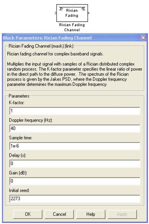
Параметр K-factor определяет
отношение мощности прямого луча к суммарной мощности всех отраженных лучей (K =
0 – релеевские замирания).
Параметр Doppler frequency
определяет частоту Доплера в канале связи, Гц (не рекомендуется устанавливать менее
0.1 Гц).
Параметр Sample time лучше устанавливать
равным -1.
Параметр Delay vector задает
комплекс отраженных лучей с индивидуальными задержками в секундах.
Параметр Gain vector задает амплитуды
комплекса отраженных лучей в дБ.
26.
Счетчик Ошибок – считает количество переданных битов, количество
ошибочных битов, и вероятность ошибки (BER). Блок можно извлечь из демо-схем
MATLAB: В основном окне
MATLAB зайдите в Help => Demos => Blocksets => CDMA Reference =>
IS-95 Forward Traffic Channel End-to-End (sim). Скопируйте два блока, показанные
ниже на рисунке, к себе в рабочий файл.
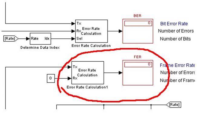
Error
Rate Calculation:
На вход Tx подается передаваемая
цифровая последовательность (амплитудные уровни «0» и «1» должны быть равны 0 и
1 соответственно; длительность бита должна состоять из одного отсчета, то есть скорость
передачи данных должна равняться частоте дискретизации цифровой последовательности).
На вход Rx подается принимаемая цифровая последовательность (условия на сигнал
– такие же как и на сигнал Tx). Обычно принимаемый сигнал Rx задержан
на несколько битовых интервалов, поэтому для достоверного сравнения Tx и
Rx сигналов параметр Receive delay должен быть равен числу бит задержки.
Computation delay – это задержка перед началом счета сравнения (Computation
delay = Receive delay).
Дисплей
Счетчика:
Верхнее окно счетчика показывает вероятность
ошибки (BER)
Среднее окно счетчика показывает количество
ошибочных бит
Нижнее окно счетчика показывает количество
передаваемых бит
27. Communication Blockset/Comm
Sinks/Discrete-Time Eye and Scatter Diagrams – отображает «глазковую диаграмму»
и комплексную плоскость входного дискретного сигнала данных. Входной сигнал может
быть как комплексным, так и действительным.
Ниже на осциллограмме изображены комплексный
(квадратурный) цифровой сигнал со скоростью передачи данных 200 бит/с (QPSK). Длительность
символа равна 0.01 с. Количество возможных позиций M равно 4. Квадратурные сигналы
отфильтрованы фильтрами нижних частот Баттерворта 8-го порядка с частотой среза
100 Гц. Частота дискретизации 1000 Гц.
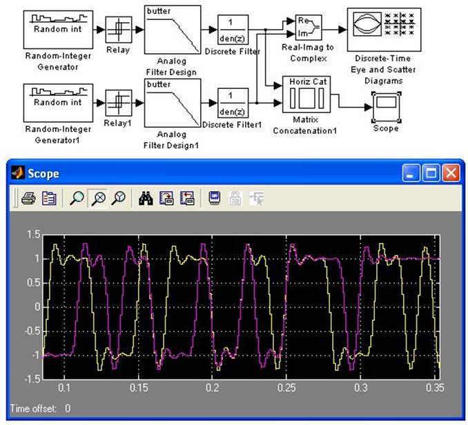
Параметр Trace period определяет
интервал построения глазковой диаграммы (обычно равен 2-3 длительности информационного
символа). Trace period = 0.03 (в примере).
Параметр Trace offset определяет
временной сдвиг глазковой диаграммы (для выставления «глазка» по центру диаграммы).
Trace offset = 0 (в примере).
Параметр Decision point определяет
местоположение сечения, по которому строятся точки на комплексной плоскости (см.
рисунок ниже – черная вертикальная линия на глазковой диаграмме). Decision
point должен быть кратен Sample time for plot update для диаграммы. Decision
point = 0.013 (в примере).
Параметр Lower and upper
bounds of diagram определяет амплитудный диапазон окна «глазковой» диаграммы.
Должен быть не меньше амплитудного коридора сигнала. Lower and upper bounds
of diagram = [-1.5 1.5] (в примере).
Параметр Number of saved
traces определяет количество одновременно прорисовываемых точек на комплексной
плоскости (или кривых на «глазковой диаграмме»). Number of saved traces
= 500 (в примере).
Параметр Diagram type = Eye and Scatter
Diagrams
Параметр Line type….. определяет цвет
линий
Sample time for plot update
– интервал дискретизации для диаграммы. Для качественной прорисовки глазковой диаграммы
Sample time for plot update лучше брать в 10 раз меньше длительности информационного
символа. Sample time for plot update = 0.001 (в примере).
Neglecting square terms of the Q function, your expression is correct, but it is the symbol error probability, not the bit error probability:
$$P_s=2.5,Qleft(frac{d}{2sigma}right)tag{1}$$
With Gray encoding, the bit error probability is closely approximated by
$$P_bapproxfrac13Pstag{2}$$
because there are $3$ bits per symbol, and the most likely symbol errors (i.e. between neighboring symbols) cause only one bit error.
Furthermore, if $N_0$ is the one-sided noise density, then $sigma=sqrt{N_0/2}$, and the energy per bit is $E_b=E_s/3$, where $E_s$ is the symbol energy. It remains to express the distance $d$ between the symbols in terms of $E_s$. The energy of the four inner symbols is $d^2/2$. The energy of the corner symbols is $5d^2/2$. So for equally probable symbols, the average symbol energy is
$$E_s=frac12cdotfrac{d^2}{2}+frac12cdotfrac{5d^2}{2}=frac{3d^2}{2}tag{3}$$
which gives
$$d=sqrt{frac{2E_s}{3}}=sqrt{2E_b}tag{4}$$
Plugging (4) into (1) gives for the symbol error probablity
$$P_s=2.5,Qleft(sqrt{frac{E_b}{N_0}}right)tag{5}$$
which, combined with (2), gives for the average bit error probability
$$E_bapproxfrac{5}{6},Qleft(sqrt{frac{E_b}{N_0}}right)tag{6}$$
Note that Eq. (6) for the bit error probability was derived under the assumption that the SNR is relatively high. This assumption is implicit in Eq. (1), where quadratic terms of the Q function were neglected. The exact expression for the symbol error probability is
$$P_s=2.5,Qleft(frac{d}{2sigma}right)-1.5,Q^2left(frac{d}{2sigma}right)tag{a}$$
For $d/2sigmarightarrow 0$ the expression (a) approaches $7/8$. This is a consequence of all symbols being detected with equal probability, and since only one of them is the correct symbol, the symbol error probability must be $7/8$.
The expression (2) for the bit error probability assumes that each symbol error causes only one bit error, which is true if Gray encoding is used and if it is assumed that symbol errors only occur between neighboring symbols, the latter being a reasonable assumption at relatively high SNRs. However, for $d/2sigmarightarrow 0$ any symbol will be confused with any other with equal probability. There is only one symbol (the correct one) where there are zero bit errors. There are $3$ symbols causing one bit error, $3$ symbols causing $2$ bit errors, and one symbol causing $3$ bit errors. Since for very bad SNRs all symbols are detected with equal probability, the average number of wrong bits per detected symbol is
$$frac18cdot 0+frac{3}{8}cdot 1+frac{3}{8}cdot 2+frac18cdot 3=frac{3}{2}$$
And since there are $3$ bits per symbol, the average bit error rate for $d/2sigmarightarrow 0$ is
$$E_b=frac{3}{2}cdotfrac13=frac12$$
as expected.