Фильтр Калмана — это легко
Время прочтения
18 мин
Просмотры 48K

Много людей, в первый раз сталкивающихся в работе с датчиками, склонны считать, что получаемые показания — это точные значения. Некоторые вспоминают, что в показаниях всегда есть погрешности и ошибки. Чтобы ошибки в измерениях не приводили к ошибкам в функционировании системы в целом, данные датчиков необходимо обрабатывать. На ум сразу приходит словосочетание “фильтр Калмана”. Но слава этого “страшного” алгоритма, малопонятные формулы и разнообразие используемых обозначений отпугивают разработчиков. Постараемся разобраться с ним на практическом примере.
Об алгоритме
Что же нам потребуется для работы фильтра Калмана?
- Нам потребуется модель системы.
- Модель должна быть линейной (об этом чуть позже).
- Нужно будет выбрать переменные, которые будут описывать состояние системы (“вектор состояния”).
- Мы будем производить измерения и вычисления в дискретные моменты времени (например, 10 раз в секунду). Нам потребуется модель наблюдения.
- Для работы фильтра достаточно данных измерений в текущий момент времени и результатов вычислений с предыдущего момента времени.
Алгоритм работает итеративно. На каждом шаге алгоритм берёт данные датчиков (с шумом и другими проблемами), вектор состояния с предыдущего шага и по этим данным оценивает состояние системы на текущем шаге. Кроме того, он еще отслеживает насколько мы можем быть уверены, что наш текущий вектор состояний соответствует истинному положению дел (разброс значений для каждой переменной в векторе).
Обычно используются следующие обозначения:
 — вектор состояния;
 — мера неопределенности вектора состояния. Представляет из себя ковариационную матрицу (об этом позже — это будет, наверное, самая сложная часть).
Содержимое вектора состояния зависит от фантазии разработчика и решаемой задачи. Например, мы можем отслеживать координаты объекта, а также его скорость и ускорение. В этом случае получается вектор из трёх переменных: {позиция, скорость, ускорение} (для одномерного случая; для 3D мира будет по одному такому набору для каждой оси, то есть, 9 значений в векторе)
По сути, речь идёт о совместном распределении случайных величин
В фильтре Калмана мы предполагаем, что все погрешности и ошибки (как во входных данных, так и в оценке вектора состояния) имеют нормальное распределение. А для многомерного нормального распределения его полностью определяют два параметра: математическое ожидание вектора и его ковариационная матрица.
Математическая модель системы / процесса
Мы имеем дело с динамической системой, т.е. состояние системы меняется со временем. Имея модель системы, фильтр Калмана может предугадывать, каким будет состояние системы в следующий момент времени. Именно это позволяет фильтру так эффективно устранять шум и оценивать параметры, которые не наблюдаются (не измеряются) напрямую.
Фильтр Калмана накладывает ограничения на используемые модели: это должны быть дискретные модели в пространстве состояний. А ещё они должны быть линейными.
Дискретные и линейные?
Дискретность означает для нас то, что модель работает “шагами”. На каждом шаге мы вычисляем новое состояние системы по вектору состояния с предыдущего шага. Обычно, модели такого рода задаются системой разностных уравнений.
По поводу линейности: каждое уравнение системы является линейным уравнением, задающим новое значение переменной состояния. Т.е. никаких косинусов, синусов, возведений в степень и даже сложений с константой.
Такую модель удобно представлять в виде разностного матричного уравнения:

Давайте разберём это уравнение подробно. В первую очередь, нас интересует первое слагаемое ( ) — это как раз модель эволюции процесса. А матрица
  (также встречаются обозначения
  ,
,  ) — называется матрицей процесса (state transition matrix). Она задаёт систему линейных уравнений, описывающих, как получается новое состояние системы из предыдущего.
Например, для равноускоренного движения матрица будет выглядеть так:

Первая строка матрицы — хорошо знакомое уравнение  . Аналогично, вторая строка матрицы описывает изменение скорости. Третья строка описывает изменение ускорения.
А что же с остальными слагаемыми?
В некоторых случаях, мы напрямую управляем процессом (например, управляем квадракоптером с помощью пульта Д/У) и нам достоверно известны задаваемые параметры (заданная на пульте скорость полёта). Второе слагаемое — это модель управления. Матрица  называется матрицей управления, а вектор
  — вектор управляющих воздействий. В случаях когда мы только наблюдаем за процессом, это слагаемое отсутствует.
Последнее слагаемое —  — это вектор ошибки модели. Модель равноускоренного движения абсолютно точно описывает положение объекта. Однако в реальном мире есть множество случайных факторов — дороги неровные, дует ветер, и т.п. Иногда, процесс сложен и приходится использовать упрощённую модель, которая не учитывает все аспекты. Именно так возникает ошибка модели.
То, что мы записываем это слагаемое, не означает, что мы знаем ошибку на каждом шаге или описываем её аналитически. Однако фильтр Калмана делает важное предположение — ошибка имеет нормальное распределение с нулевым математическим ожиданием и ковариационной матрицей  . Эта матрица очень важна для стабильной работы фильтра и мы её рассмотрим позже.
Модель наблюдения
Не всегда получается так, что мы измеряем интересующие нас параметры напрямую (например, мы измеряем скорость вращения колеса, хотя нас интересует скорость автомобиля). Модель наблюдения описывает связь между переменными состояния и измеряемыми величинами:

 — это вектор измерения/наблюдения.Это значения, получаемые с датчиков системы.
Первое слагаемое  — модель, связывающая вектор состояния с соответствующими ему показаниями датчиков. (Такой выбор модели может показаться странным, ведь наша задача — получить из , а эта модель получает из . Но это действительно так. В частности, это необходимо потому, что некоторые переменные состояния из могут отсутствовать в ).
Второе слагаемое  — это вектор ошибок измерения. Как и в случае с предыдущими ошибками, предполагается, что она имеет нормальное распределение с нулевым математическим ожиданием.
  — ковариационная матрица, соответствующая вектору .
Вернёмся к нашему примеру. Пусть у нас на роботе установлен один единственный датчик — GPS приёмник (“измеряет” положение). В этом случае матрица  будет выглядеть следующим образом:

Строки матрицы соответствуют переменным в векторе состояния, столбцы — элементам вектора измерений. В первой строке матрицы находится значение “1” так как единица измерения положения в векторе состояния совпадает с единицей измерения значения в векторе измерений. Остальные строки содержат “0” потому что переменные состояния соответствующие этим строкам не измеряются датчиком.
Что будет, если датчик и модель используют разные единицы измерения? А если датчиков несколько?
Например, модель использует метры, а датчик — количество оборотов колеса. В этом случае матрица будет выглядеть так:

Количество датчиков ничем (кроме здравого смысла) не ограничено.
Например, добавим спидометр:

Второй столбец матрицы соответствует нашему новому датчику.
Несколько датчиков могут измерять один и тот же параметр. Добавим ещё один датчик скорости:

Ковариационные матрицы и где они обитают
Для настройки фильтра нам потребуется заполнить несколько ковариационных матриц:
, и .
Ковариационные матрицы?
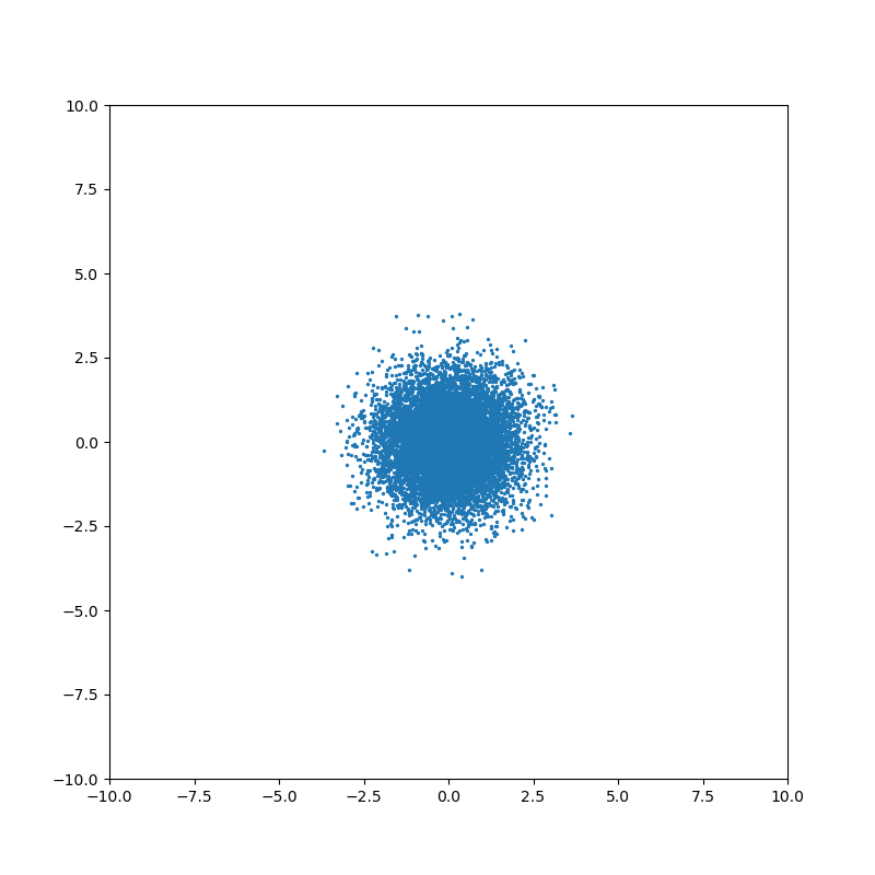
Для нормально распределенной случайной величины её математическое ожидание и дисперсия полностью определяют её распределение. Дисперсия — это мера разброса случайной величины. Чем больше дисперсия — тем сильнее может отклоняться случайная величина от её математического ожидания. Ковариационная матрица — это многомерный аналог дисперсии, для случая, когда у нас не одна случайная величина, а случайный вектор.
В одной статье сложно уместить всю теорию вероятностей, поэтому ограничимся сугубо практическими свойствами ковариационных матриц. Это симметричные квадратные матрицы, на главной диагонали которой располагаются дисперсии элементов вектора. Остальные элементы матрицы — ковариации между компонентами вектора. Ковариация показывает, насколько переменные зависят друг от друга.
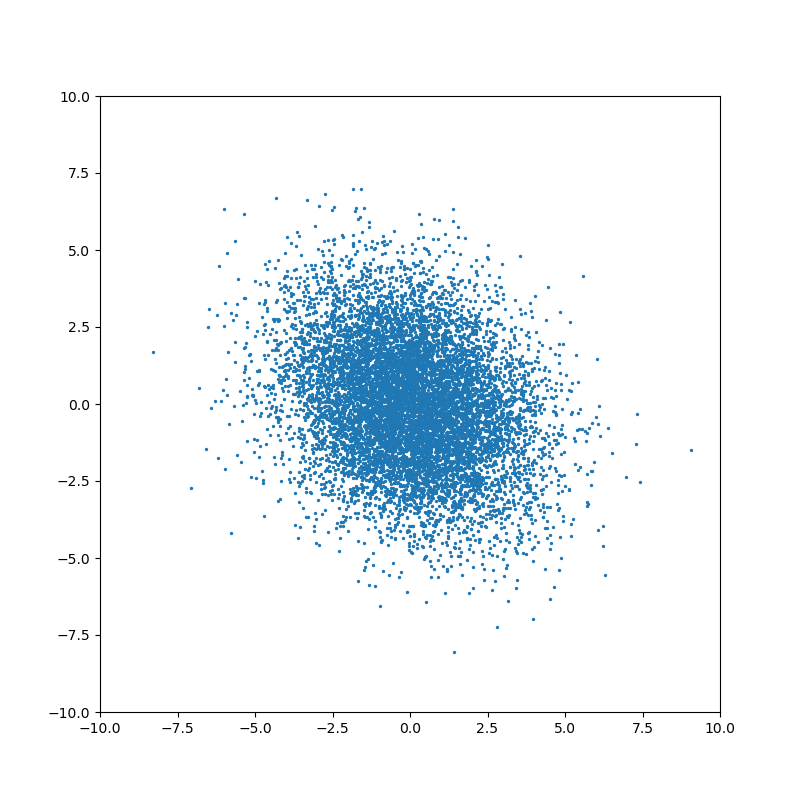
Проиллюстрируем влияние мат. ожидания, дисперсии и ковариации.
Начнём с одномерного случая. Функция плотности вероятности нормального распределения — знаменитая колоколообразная кривая. Горизонтальная ось — значение случайной величины, а вертикальная ось — сравнительная вероятность того что случайная величина примет это значение:

Чем меньше дисперсия — тем меньше ширина колокола.
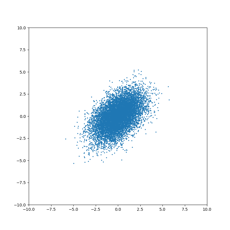
Понятие ковариации возникает для совместного распределения нескольких случайных величин. Когда случайные величины независимы, то ковариация равна нулю:

Ненулевое значение ковариации означает, что существует связь между значениями случайных величин:


На каждом шаге фильтр Калмана строит предположение о состоянии системы, исходя из предыдущей оценки состояния и данных измерений. Если неопределенности вектора состояния выше, чем ошибка измерения, то фильтр будет выбирать значения ближе к данным измерений. Если ошибка измерения больше оценки неопределенности состояния, то фильтр будет больше “доверять” данным моделирования. Именно поэтому важно правильно подобрать значения ковариационных матриц — основного инструмента настройки фильтра.
Рассмотрим каждую матрицу подробнее:
— ковариационная матрица состояния
Квадратная матрица, порядок матрицы равен размеру вектора состояния
Как уже было сказано выше, эта матрица определяет “уверенность” фильтра в оценке переменных состояния. Алгоритм самостоятельно обновляет эту матрицу в процессе работы. Однако нам нужно установить начальное состояние, вместе с исходным предположением о векторе состояния.
Во многих случаях нам неизвестны значения ковариации между переменными для изначального состояния (элементы матрицы, расположенные вне главной диагонали). Поэтому можно проигнорировать их, установив равными 0. Фильтр самостоятельно обновит значения в процессе работы. Если же значения ковариации известны, то, конечно же, стоит использовать их.
Дисперсию же проигнорировать не выйдет. Необходимо установить значения дисперсии в зависимости от нашей уверенности в исходном векторе состояния. Для этого можно воспользоваться правилом трёх сигм: значение случайной величины попадает в диапазон  с вероятностью 99.7%.
Пример
Допустим, нам нужно установить дисперсию для переменной состояния — скорости робота. Мы знаем что максимальная скорость передвижения робота — 10 м/с. Но начальное значение скорости нам неизвестно. Поэтому, мы выберем изначальное значение переменной — 0 м/с, а среднеквадратичное отклонение  ;
;  Соответственно, дисперсия
  .
.
— ковариационная матрица шума измерений
Квадратная матрица, порядок матрицы равен размеру вектора наблюдения (количеству измеряемых параметров).
Во многих случаях можно считать, что измерения не коррелируют друг с другом. В этом случае матрица будет являться диагональной матрицей, где все элементы вне главной диагонали равны нулю. Достаточно будет установить значения дисперсии для каждого измеряемого параметра. Иногда эти данные можно найти в документации к используемым датчика. Однако, если справочной информации нет, то можно оценить дисперсию, измеряя датчиком заранее известное эталонное значение, или воспользоваться правилом трёх сигм.
— ковариационная матрица ошибки модели
Квадратная матрица, порядок матрицы равен размеру вектора состояния.
С этой матрицей обычно возникает наибольшее количество вопросов. Что означает ошибка модели? Каков смысл этой матрицы и за что она отвечает? Как заполнять эту матрицу? Рассмотрим всё по порядку.
Каждый раз, когда фильтр предсказывает состояние системы, используя модель процесса, он увеличивает неуверенность в оценке вектора состояния. Для одномерного случая формула выглядит приблизительно следующим образом:

Если установить очень маленькое значение , то этап предсказания будет слабо увеличивать неопределенность оценки. Это означает, что мы считаем, что наша модель точно описывает процесс.
Если же установить большое значение , то этап предсказания будет сильно увеличивать неопределенность оценки. Таким образом, мы показываем что модель может содержать неточности или неучтенные факторы.
Для многомерного случая формула выглядит несколько сложнее, но смысл схожий. Однако, есть важное отличие: эта матрица указывает, на какие переменные состояния будут в первую очередь влиять ошибки модели и неучтённые факторы.
Допустим, мы отслеживаем перемещение робота, используя модель равноускоренного движения, и вектор состояния содержит следующие переменные: положение x, скорость v и ускорение a. Однако, наша модель не учитывает, что на дороге встречаются неровности.
Когда робот проходит неровность, показания датчиков и предсказание модели начнут расходиться. Структура матрицы будет определять, как фильтр отреагирует на это расхождение.
Мы можем выдвинуть различные предположения относительно природы шума. Для нашего примера с равноускоренным движением логично было бы предположить, что неучтённые факторы (неровность дороги) в первую очередь влияют на ускорение. Этот подход применим ко многим структурам модели, где в векторе состояния присутствует переменная и несколько её производных по времени (например, положение и производные: скорость и ускорение). Матрица выбирается таким образом, чтобы наибольшее значение соответствовало самому высокому порядку производной.
Так как же заполняется матрица Q?
Обычно используют модель-приближение. Рассмотрим на примере модели равноускоренного движения:
Модель непрерывного белого шума
Мы предполагаем, что ускорение постоянно на каждом шаге. Но из-за неровностей дороги ускорение, на самом деле, постоянно изменяется. Мы можем предположить, что изменение ускорения происходит под воздействием непрерывного белого шума с нулевым математическим ожиданием (т.е. усреднив все небольшие изменения ускорения за время движения робота мы получаем 0)
В этой модели матрица Q рассчитывается следующим образом

Мы формируем матрицу Qc в соответствии со структурой вектора состояния. Наивысшему порядку производной соответствует правый нижний элемент матрицы. В случае, если в векторе состояния несколько таких переменных, то каждая из них учитывается в матрице.
Для нашей модели равноускоренного движения матрица будет выглядеть так:

 — спектральная плотность мощности белого шума
Подставляем матрицу процесса, соответствующую нашей модели:

После перемножения и интегрирования получаем:

Модель “кусочного” белого шума
Мы предполагаем, что ускорение на самом деле постоянно в течение каждого шага моделирования, но дискретно и независимо меняется между шагами. Выглядит очень похоже на предыдущую модель, но небольшая разница есть

 — мощность шума
 — наивысший порядок производной, используемой в модели (т.е. ускорение для вышеописанной модели)
В этой модели матрица определяется следующим образом:
![$ Q = mathbb{E}[,Gammaomega(t)omega(t)Gamma^T],=Gammasigma_upsilon^2Gamma^T $](https://habrastorage.org/getpro/habr/formulas/68f/0bb/a32/68f0bba3267049b97faff063484e96eb.svg)
Из матрицы процесса F
берём столбец с наивысшим порядком производной

и подставляем в формулу. В итоге получаем:

Обе модели являются приближениями того, что происходит на самом деле в реальности. На практике, приходится экспериментировать и выяснять, какая модель подходит лучше в каждом отдельном случае. Плюсом второй модели является то, что мы оперируем дисперсией шума, с которой уже хорошо умеем работать.
Простейший подход
В некоторых случаях прибегают к грубому упрощению: устанавливают все элементы матрицы равными нулю, за исключением элементов, соответствующих максимальным порядкам производных переменных состояния.
Действительно, если рассчитать по одному из приведённых выше методов, при достаточно малых значениях  , значения элементов матрицы оказываются очень близкими к нулю.
Т.е. для нашей модели равноускоренного движения можно взять матрицу следующего вида:

И хотя такой подход не совсем корректен, его можно использовать в качестве первого приближения или для экспериментов. Без сомнения, не стоит выбирать матрицу таким образом для любых важных задач без весомых причин.
Важное замечание
Во всех примерах выше используется вектор состояния  и может показаться, что во всех случаях дисперсия, соответствующая наивысшему порядок производной, находится в правом нижнем углу матрицы. Это не так.
Рассмотрим вектор состояния 
Матрица будет представлять собой блочную матрицу, где отдельные блоки 3х3 элементов будут соответствовать группам и  . Остальные элементы матрицы будут равны нулю.
Дисперсия, соответствующая наивысшим порядкам производных  и
и  , будет находиться на 3-ей и 5-ой позициях на главной диагонали матрицы.
Однако, на практике нет никакого смысла перемешивать порядок переменных состояния таким образом, чтобы порядки производных шли не по очереди — это просто неудобно.
Пример кода
Нет смысла изобретать велосипед и писать свою собственную реализацию фильтра Калмана, когда существует множество готовых библиотек. Я выбрал язык python и библиотеку filterpy для примера.
Чтобы не загромождать пример, возьмем одномерный случай. Одномерный робот оборудован одномерным GPS, который определяет положение с некоторой погрешностью.
Моделирование данных датчиков
Начнём с равномерного движения:
Simulator.py
import numpy as np
import numpy.random

# Моделирование данных датчика
def simulateSensor(samplesCount, noiseSigma, dt):
   # Шум с нормальным распределением. мат. ожидание = 0, среднеквадратичное отклонение = noiseSigma
   noise = numpy.random.normal(loc = 0.0, scale = noiseSigma, size = samplesCount)

   trajectory = np.zeros((3, samplesCount))

   position = 0
   velocity = 1.0
   acceleration = 0.0

   for i in range(1, samplesCount):
       position = position + velocity * dt + (acceleration * dt ** 2) / 2.0
       velocity = velocity + acceleration * dt
       acceleration = acceleration

       trajectory[0][i] = position
       trajectory[1][i] = velocity
       trajectory[2][i] = acceleration

   measurement = trajectory[0] + noise

   return trajectory, measurement # Истинное значение и данные "датчика" с шумом
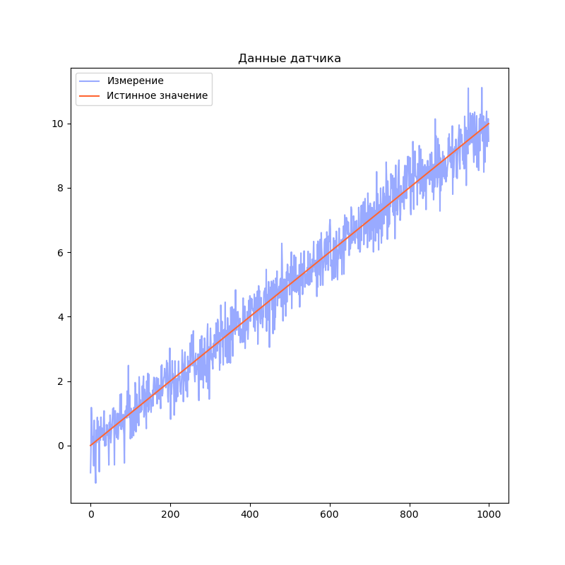
Визуализируем результаты моделирования:
Код
import matplotlib.pyplot as plt
dt = 0.01
measurementSigma = 0.5
trajectory, measurement = simulateSensor(1000, measurementSigma, dt)

plt.title("Данные датчика")
plt.plot(measurement, label="Измерение", color="#99AAFF")
plt.plot(trajectory[0], label="Истинное значение", color="#FF6633")
plt.legend()
plt.show()
Реализация фильтра
Для начала выберем модель системы. Я решил взять 3 переменных состояния: положение, скорость и ускорение. В качестве модели процесса возьмем модель равноускоренного движения:
У нас единственный датчик, который напрямую измеряет положение. Поэтому модель наблюдения получается очень простой:

Мы предполагаем, что наш робот находится в точке 0 и имеет нулевые скорость и ускорение в начальный момент времени:

Однако, мы не уверены, что это именно так. Поэтому установим матрицу ковариации для начального состояния с большими значениями на главной диагонали:

Я воспользовался функцией библиотеки filterpy для расчёта ковариационной матрицы ошибки модели: filterpy.common.Q_discrete_white_noise. Эта функция использует модель непрерывного белого шума.
Код
import filterpy.kalman
import filterpy.common
import matplotlib.pyplot as plt
import numpy as np
import numpy.random
from Simulator import simulateSensor # моделирование датчиков
dt = 0.01 # Шаг времени
measurementSigma = 0.5 # Среднеквадратичное отклонение датчика
processNoise = 1e-4 # Погрешность модели
# Моделирование данных датчиков
trajectory, measurement = simulateSensor(1000, measurementSigma, dt)
# Создаём объект KalmanFilter
filter = filterpy.kalman.KalmanFilter(dim_x=3, # Размер вектора стостояния
dim_z=1) # Размер вектора измерений
# F - матрица процесса - размер dim_x на dim_x - 3х3
filter.F = np.array([ [1, dt, (dt**2)/2],
[0, 1.0, dt],
[0, 0, 1.0]])
# Матрица наблюдения - dim_z на dim_x - 1x3
filter.H = np.array([[1.0, 0.0, 0.0]])
# Ковариационная матрица ошибки модели
filter.Q = filterpy.common.Q_discrete_white_noise(dim=3, dt=dt, var=processNoiseVariance)
# Ковариационная матрица ошибки измерения - 1х1
filter.R = np.array([[measurementSigma*measurementSigma]])
# Начальное состояние.
filter.x = np.array([0.0, 0.0, 0.0])
# Ковариационная матрица для начального состояния
filter.P = np.array([[10.0, 0.0, 0.0],
[0.0, 10.0, 0.0],
[0.0, 0.0, 10.0]])
filteredState = []
stateCovarianceHistory = []
# Обработка данных
for i in range(0, len(measurement)):
z = [ measurement[i] ] # Вектор измерений
filter.predict() # Этап предсказания
filter.update(z) # Этап коррекции
filteredState.append(filter.x)
stateCovarianceHistory.append(filter.P)
filteredState = np.array(filteredState)
stateCovarianceHistory = np.array(stateCovarianceHistory)
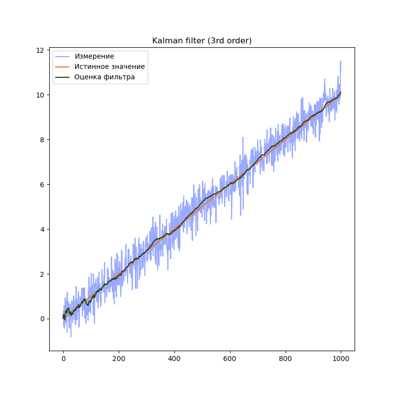
# Визуализация
plt.title("Kalman filter (3rd order)")
plt.plot(measurement, label="Измерение", color="#99AAFF")
plt.plot(trajectory[0], label="Истинное значение", color="#FF6633")
plt.plot(filteredState[:, 0], label="Оценка фильтра", color="#224411")
plt.legend()
plt.show()
Бонус — сравнение различных порядков моделей
Сравним поведение фильтра с моделями разного порядка. Для начала, смоделируем более сложный сценарий поведения робота. Пусть робот находится в покое первые 20% времени, затем движется равномерно, а затем начинает двигаться равноускоренно:
Simulator.py
# Моделирование данных датчика
def simulateSensor(samplesCount, noiseSigma, dt):
   # Шум с нормальным распределением. мат. ожидание = 0, среднеквадратичное отклонение = noiseSigma
   noise = numpy.random.normal(loc = 0.0, scale = noiseSigma, size = samplesCount)

   trajectory = np.zeros((3, samplesCount))

   position = 0
   velocity = 0.0
   acceleration = 0.0

   for i in range(1, samplesCount):
       position = position + velocity * dt + (acceleration * dt ** 2) / 2.0
       velocity = velocity + acceleration * dt
       acceleration = acceleration

       # Переход на равномерное движение
       if(i == (int)(samplesCount * 0.2)):
           velocity = 10.0

       # Переход на равноускоренное движение
       if (i == (int)(samplesCount * 0.6)):
           acceleration = 10.0

       trajectory[0][i] = position
       trajectory[1][i] = velocity
       trajectory[2][i] = acceleration

   measurement = trajectory[0] + noise

   return trajectory, measurement # Истинное значение и данные "датчика" с шумом
В предыдущем примере мы использовали модель, содержащую переменную (положение) и две производных её по времени (скорость и ускорение). Посмотрим, что будет, если избавиться от одной или обеих производных:
2-й порядок
# Создаём объект KalmanFilter
filter = filterpy.kalman.KalmanFilter(dim_x=2,      # Размер вектора стостояния
                                     dim_z=1)      # Размер вектора измерений

# F - матрица процесса - размер dim_x на dim_x - 2х2
filter.F = np.array([ [1,   dt],
                     [0,   1.0]])


# Матрица наблюдения - dim_z на dim_x - 1x2
filter.H = np.array([[1.0, 0.0]])

filter.Q = [[dt**2,       dt],
           [   dt,      1.0]] * processNoise

# Начальное состояние.
filter.x = np.array([0.0, 0.0])

# Ковариационная матрица для начального состояния
filter.P = np.array([[8.0, 0.0],
                    [0.0, 8.0]])
1-й порядок
# Создаём объект KalmanFilter
filter = filterpy.kalman.KalmanFilter(dim_x=1,      # Размер вектора стостояния
                                     dim_z=1)      # Размер вектора измерений

# F - матрица процесса - размер dim_x на dim_x - 1х1
filter.F = np.array([ [1.0]])


# Матрица наблюдения - dim_z на dim_x - 1x1
filter.H = np.array([[1.0]])

# Ковариационная матрица ошибки модели
filter.Q = processNoise

# Ковариационная матрица ошибки измерения - 1х1
filter.R = np.array([[measurementSigma*measurementSigma]])

# Начальное состояние.
filter.x = np.array([0.0])

# Ковариационная матрица для начального состояния
filter.P = np.array([[8.0]])
Сравним результаты:
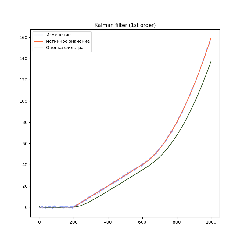
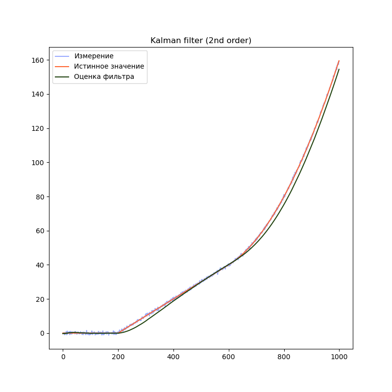

На графиках сразу заметно, что модель первого порядка начинает отставать от истинного значения на участках равномерного движения и равноускоренного движения. Модель второго порядка успешно справляется с участком равномерного движения, но так же начинает отставать на участке равноускоренного движения. Модель третьего порядка справляется со всеми тремя участками.
Однако, это не означает что нужно использовать модели высокого порядка во всех случаях. В нашем примере, модель третьего порядка справляется с участком равномерного движения несколько хуже модели второго порядка, т.к. фильтр интерпретирует шум сенсора как изменение ускорения. Это приводит к колебанию оценки фильтра. Стоит подбирать порядок модели в соответствии с планируемыми режимами работы фильтра.
Нелинейные модели и фильтр Калмана
Почему фильтр Калмана не работает для нелинейных моделей и что делать
Всё дело в нормальном распределении. При применении линейных преобразованийк нормально распределенной случайной величине, результирующее распределение будет представлять собой нормальное распределение, или будет пропорциональным нормальному распределению. Именно на этом принципе и строится математика фильтра Калмана.
Есть несколько модификаций алгоритма, которые позволяют работать с нелинейными моделями.
Например:
Extended Kalman Filter (EKF) — расширенный фильтр Калмана. Этот подход строит линейное приближение модели на каждом шаге. Для этого требуется рассчитать матрицу вторых частных производных функции модели, что бывает весьма непросто. В некоторых случаях, аналитическое решение найти сложно или невозможно, и поэтому используют численные методы.
Unscented Kalman Filter (UKF). Этот подход строит приближение распределения получающегося после нелинейного преобразования при помощи сигма-точек. Преимуществом этого метода является то, что он не требует вычисления производных.
Мы рассмотрим именно Unscented Kalman Filter
Unscented Kalman Filter и почему он без запаха
Основная магия этого алгоритма заключается в методе, который строит приближение распределения плотности вероятности случайной величины после прохождения через нелинейное преобразование. Этот метод называется unscented transform — сложнопереводимое на русский язык название. Автор этого метода, Джеффри Ульман, не хотел, чтобы его разработку называли “Фильтр Ульмана”. Согласно интервью, он решил назвать так свой метод после того как увидел дезодорант без запаха (“unscented deodorant”) на столе в лаборатории, где он работал.
Этот метод достаточно точно строит приближение функции распределения случайной величины, но что более важно — он очень простой.
Для использования UKF не придётся реализовывать какие-либо дополнительные вычисления, за исключением моделей системы. В общем виде, нелинейная модель не может быть представлена в виде матрицы, поэтому мы заменяем матрицы и на функции  и
и  . Однако смысл этих моделей остаётся тем же.
Реализуем unscented Kalman filter для линейной модели из прошлого примера:
Код
import filterpy.kalman
import filterpy.common
import matplotlib.pyplot as plt
import numpy as np
import numpy.random
from Simulator import simulateSensor, CovarianceQ

dt = 0.01
measurementSigma = 0.5
processNoiseVariance = 1e-4

# Функция наблюдения - аналог матрицы наблюдения
# Преобразует вектор состояния x в вектор измерений z
def measurementFunction(x):
   return np.array([x[0]])

# Функция процесса - аналог матрицы процесса
def stateTransitionFunction(x, dt):
   newState = np.zeros(3)
   newState[0] = x[0] + dt * x[1] + ( (dt**2)/2 ) * x[2]
   newState[1] = x[1] + dt * x[2]
   newState[2] = x[2]

   return newState


trajectory, measurement = simulateSensor(1000, measurementSigma)

# Для unscented kalman filter необходимо выбрать алгоритм выбора сигма-точек
points = filterpy.kalman.JulierSigmaPoints(3, kappa=0)

# Создаём объект UnscentedKalmanFilter
filter = filterpy.kalman.UnscentedKalmanFilter(dim_x = 3,
                                              dim_z = 1,
                                              dt = dt,
                                              hx = measurementFunction,
                                              fx = stateTransitionFunction,
                                              points = points)


# Ковариационная матрица ошибки модели
filter.Q = filterpy.common.Q_discrete_white_noise(dim=3, dt=dt, var=processNoiseVariance)

# Ковариационная матрица ошибки измерения - 1х1
filter.R = np.array([[measurementSigma*measurementSigma]])

# Начальное состояние.
filter.x = np.array([0.0, 0.0, 0.0])

# Ковариационная матрица для начального состояния
filter.P = np.array([[10.0, 0.0,  0.0],
                    [0.0,  10.0, 0.0],
                    [0.0,  0.0,  10.0]])

filteredState = []
stateCovarianceHistory = []

for i in range(0, len(measurement)):
   z = [ measurement[i] ]
   filter.predict()
   filter.update(z)

   filteredState.append(filter.x)
   stateCovarianceHistory.append(filter.P)

filteredState = np.array(filteredState)
stateCovarianceHistory = np.array(stateCovarianceHistory)

plt.title("Unscented Kalman filter")
plt.plot(measurement, label="Измерение", color="#99AAFF")
plt.plot(trajectory[0], label="Истинное значение", color="#FF6633")
plt.plot(filteredState[:, 0], label="Оценка фильтра", color="#224411")
plt.legend()
plt.show()
Разница в коде минимальна. Мы заменили матрицы F и H на функции f(x) и h(x). Это позволяет использовать нелинейные модели системы и/или наблюдения:
# Функция наблюдения - аналог матрицы наблюдения
# Преобразует вектор состояния x в вектор измерений z
def measurementFunction(x):
   return np.array([x[0]])

# Функция процесса - аналог матрицы процесса
def stateTransitionFunction(x, dt):
   newState = np.zeros(3)
   newState[0] = x[0] + dt * x[1] + ( (dt**2)/2 ) * x[2]
   newState[1] = x[1] + dt * x[2]
   newState[2] = x[2]

   return newState
Также, появилась строчка, устанавливающая алгоритм генерации сигма-точек
points = filterpy.kalman.JulierSigmaPoints(3, kappa=0)
Этот алгоритм определяет точность оценки распределения вероятности при прохождении через нелинейное преобразование. К сожалению, существуют только общие рекомендации относительно генерации сигма-точек. Поэтому для каждой отдельной задачи значения параметров алгоритма подбираются экспериментальным путём.
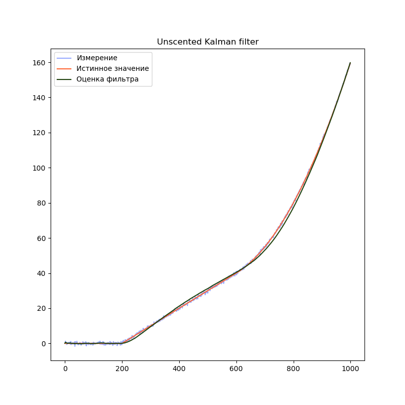
Ожидаемый результат — график оценки положения практически не отличается от обычного фильтра Калмана.
В этом примере используется линейная модель. Однако мы могли бы использовать нелинейные функции. Например, мы могли бы использовать следующую реализацию:
g = 9.8
# Вектор состояния - угол наклона
# Вектор измерений - ускорение вдоль осей X и Y
def measurementFunction(x):
  measurement = np.zeros(2)
  measurement[0] = math.sin(x[0]) * g
  measurement[1] = math.cos(x[0]) * g
  return measurement
Такую модель измерений было бы невозможно использовать в случае с линейным фильтром Калмана
Вместо заключения
За рамками статьи остались теоретические основы фильтра Калмана. Однако объем материала по этой теме ошеломляет. Сложно выбрать хороший источник. Я бы хотел рекомендовать замечательную книгу от автора библиотеки filterpy Roger Labbe (на английском языке). В ней доступно описаны принципы работы алгоритма и сопутствующая теория. Книга представляет собой документ Jupyter notebook, который позволяет в интерактивном режиме экспериментировать с примерами.
Литература
→ Roger Labbe — Kalman and Bayesian Filters in Python
→ Wikipedia
A “quick” review of Error State — Extended Kalman Filter
Recently in my job I had to work on implementing a Kalman Filter. My surprise was that there is an incredible lack of resources explaining with detail how Kaman Filter (KF) works. Imagine now the lack of resources explaining a more complex KF as the Error-state Extended Kaman Filter (ES-EKF). In this post, I will focus on the ES-EKF and leave UKF alone for now. One of the only blogs regarding a linear KF worth reading is kalman filter with images which I recommended. Here I will cover with more details the whole linear Kalman filter equations and how to derive them. After that, I will explain how to transform it into an Extended KF (EKF) and then how to transform it into an Error-state Extended KF (ES-EKF).
Notation
We will use Proper Euler angles to note rotations, that will be is (alpha, beta, gamma), we are only interested in 2D rotations, therefore, we will use the z-x’-z’’ representation in which (alpha) represents the yaw (the representation does not matter as far as the first rotation happens in the (z) axis). The steering angle will be noted by (delta).
Explanation
The Kalman Filter is used to keep track of certain variables and fuse information coming from other sensors such as Inertial Measurement Unit (IMU) or Wheels or any other sensor. It is very common in robotics because it fuses the information according to how certain the measurements are. Therefore we can have several sources of information, some more reliable than others and a KF takes that into account to keep track of the variables we are interested in.
The state (s_t) we are interested in tracking is composed by (x) and (y) coordinates, the heading of the vehicle or the yaw (theta), the current velocity (v) and steering angle (delta). The tracked orientation is only composed by the yaw (theta), we are only modelling a 2D world, therefore we do not care about the roll (beta) or pitch (gamma). And finally, we added the steering angle (delta) which is important to predict the movement of the car. Therefore the state in timestep (t) is
[s_t= left[begin{matrix}
x\y\theta\v\delta
end{matrix}right]]
KF can be divided into two steps, update and predict step. In the predict step, using the tracked information we predict where will the object move in the next step. In the update step, we update the belief we have about the variables using the external measurements coming from the sensors.
Sensor
Keep in mind that a KF can handle any number of sensors, so far we are going to use the localization measurement coming from a GPS + pseudo-gyro.
This measurement contains the global measurements ((x,y)) that avoid the system of drifting. This system (without global variables) is also called Dead reckoning. Dead reckoning or using a Kalman Filter without a global measurement is prone to cumulative errors, that means that the state will slowly diverge from the true value.
Prediction Step
We will track the state as a multivariable Gaussian distribution with mean (mu) and covariance (P). (mu_t) will be the expected value of the state using the information available (i.e. the mean of (s_t)). And the state will have a covariance matrix (P) which means how certain we are about our prediction. We will use (mu_{t-1}) and (u) to predict (mu_t). Here (u) is a control column-vector of any extra information we can use, for example, steering angle if we can have access to the steering of the car or the acceleration if we have access to it. (u) can be a vector of any size.
We will try to model everything using matrices but for now, we will use scalars, the new value of the state in (t) will be
[begin{align}
x_t &= x_{t-1} + vDelta t cos theta\
y_t &= y_{t-1} + vDelta t sin theta\
theta &= theta_{t-1}\
v_t &= v_{t-1}\
delta_t &= delta_{t-1}
end{align}]
Here we are making simplifying assumptions about the world. First, the velocity (v) and the steering (delta) of the next step will be the same as before which is a weak assumption. The strong assumption is that the heading or yaw of the car (theta) is the same. Notice we are not using the steering but we still track it, it will be useful later. We can incorporate the kinematic model here to make the prediction more robust. But that will be adding non-linearities (and so far it is a linear KF). For now, let’s work with a simple environment and later on we can make things more interesting.
This prediction can be re-formulated in matrix form as
[mu_t = Fmu_{t-1} + Bu]
Where (u) is a zero vector and (B) is a linear transformation from (u) into the same form of the state (s). Also, (F) would be ((F) has to be linear so far, in the EKF we will expand that to include non-linearities)
[F = left[begin{matrix}
1 & 0 & 0 & Delta tcostheta & 0 \
0 & 1 & 0 & Delta tsintheta & 0\
0 & 0 & 1 & 0 & 0\
0 & 0 & 0 & 1 & 0\
0 & 0 & 0 & 0 & 1
end{matrix}right]]
This will result in the same equations but using matrix notation. Rember now that we are modelling (s) as a multivariable gaussian distribution and we are keeping track of the mean (mu) of the state (s) and the covariance (P). Using the equations above we update the mean of the state, now we have to update the covariance of the state. Every time we predict we make small errors which add noise and results in a slightly less accurate prediction. The covariance (P) has to reflect this reduction in certainty. The way it is done with Gaussian distributions is that the distribution gets slightly more flat (i.e. the covariance “increase”).
In a single-variable gaussian distribution (y sim mathcal N (mu’,sigma^2)) the variance has the property that (text{var}(ky) = k^2text{var}(y)), where (k) is a scalar. In matrix notation that is (P_t = FP_{t-1}F^T). Now we have to take into account that we are adding (Bu), where (u) is the control vector and a gaussian variable with covariance (Q). The good thing about Gaussians is that the covariances of a sum of Gaussians is the sum of the covariances (if both random variables are independent). Having this into account we have.
[P_t = FP_{t-1}F^T+BQB^T]
And with this, we have finished prediction the state and updating its covariance.
Update step
In the update step, we receive a measurement (z) coming from a sensor. We use the sensor information to correct/update the belief we have about the state. The measurement is a random variable with covariance (R). This is where things get interesting. In this case, we have two Gaussians variables, the state best estimate (mu_t) and the measurement reading (z).
The best way to combine two Gaussians is by multiplying them together. By multiplying them together, if certain values have high certainty in both distributions, the result will be also a high in the product (very certain). If both values have low certainty, the product will be even lower. And if If only one is high and the other is not, then the result will lay between high and low certainty. So multiplication of Gaussians merges the information of both distributions taking into account how certain the values are (covariance).
The equations derived from multiplying two multivariate Gaussians are similar to the single variable case. We will derive them here and generalize that to matrix form.
Let’s suppose we have (x_1 sim mathcal N (mu_1,sigma_1^2)) and (x_2simmathcal N(mu_2,sigma_2^2)) (and they do not have anything to do with the state or measurement for now). Have in mind that both (x_1) and (x_2) live in the same vector space (x), therefore
[begin{align}
p(x_1) = frac 1 {sqrt{2pisigma_1^2}}e^{-frac{(x-mu_1)^2}{2sigma_2^2}} & & p(x_2) = frac 1 {sqrt{2pisigma_2^2}}e^{-frac{(x-mu_2)^2}{2sigma_2^2}}
end{align}]
by multiplying them together we obtain
[frac 1 {sqrt{2pisigma_1^2}}e^{-frac{(x-mu_1)^2}{2sigma_1^2}}frac 1 {sqrt{2pisigma_2^2}}e^{-frac{(x-mu_2)^2}{2sigma_2^2}}]
We also now about a very useful property of Gaussians: the product of Gaussians is also a gaussian distribution. Therefore, to know the result of fusing both Gaussians we have to write the equation above in a gaussian form.
[begin{align}
&=frac 1 {sqrt{2pisigma_1^2}}e^{-frac{(x-mu_1)^2}{2sigma_1^2}}frac 1 {sqrt{2pisigma_2^2}}e^{-frac{(x-mu_2)^2}{2sigma_2^2}}\
&=frac 1 {2pisigma_1^2sigma_2^2}e^{-left(frac{(x-mu_1)^2}{2sigma_1^2}+frac{(x-mu_2)^2}{2sigma_2^2}right)}\
end{align}]
Because we know the result will be a Gaussian distribution, we do not care about constant values (e.g. (2pisigma_1^2)), in fact, we only care about the exponent value, which I have to transform it into something similar to
[frac{(x-text{something})^2}{2text{something else}^2}]
Where (text{something}) will be the new mean and (text{something else}^2) will be the new covariance after multiplication. Therefore we will ignore all the other terms and focus on the exponent value.
[begin{align}
frac{(x-mu_1)^2}{2sigma_1^2}+frac{(x-mu_2)^2}{2sigma_2^2} &= frac{sigma_2^2(x-mu_1)^2+sigma_1^2(x-mu_2)^2}{2sigma_1^2sigma_2^2}\
&= frac{sigma_2^2x^2-2sigma_2^2mu_1x+sigma_2^2mu_1^2 + sigma_1^2x^2-2sigma_1^2mu_2x+sigma_1^2mu_2^2}{2sigma_1^2sigma_2^2}\
&= frac{x^2(sigma_2^2+sigma_1^2)-2x(sigma_2^2mu_1+sigma_1^2mu_2)}{2sigma_1^2sigma_2^2}+frac{sigma_2^2mu_1^2+sigma_1^2mu_2^2}{2sigma_1^2sigma_2^2}\
&= frac{(sigma_2^2+sigma_1^2)}{2sigma_1^2sigma_2^2}left(x^2-2xfrac{sigma_2^2mu_1+sigma_1^2mu_2}{sigma^2+sigma_2^2}right)+frac{sigma_2^2mu_1^2+sigma_1^2mu_2^2}{2sigma_1^2sigma_2^2}\
end{align}]
The term on the right can be ignored because it is constant and goes out of the exponent. And the term in parenthesis resembles a perfect square trinomial lacking the last squared term.
[begin{align}
&= frac{(sigma_2^2+sigma_1^2)}{2sigma_1^2sigma_2^2}left(x^2-2xfrac{sigma_2^2mu_1+sigma_1^2mu_2}{sigma^2+sigma_2^2}right)\
&= frac{(sigma_2^2+sigma_1^2)}{2sigma_1^2sigma_2^2}left(x^2-2xfrac{sigma_2^2mu_1+sigma_1^2mu_2}{sigma^2+sigma_2^2} + left(frac{sigma_2^2mu_1+sigma_1^2mu_2}{sigma^2+sigma_2^2}right)^2 — left(frac{sigma_2^2mu_1+sigma_1^2mu_2}{sigma^2+sigma_2^2}right)^2 right)\
&= frac{(sigma_2^2+sigma_1^2)}{2sigma_1^2sigma_2^2}left(left(x-frac{sigma_2^2mu_1+sigma_1^2mu_2}{sigma^2+sigma_2^2}right)^2 — left(frac{sigma_2^2mu_1+sigma_1^2mu_2}{sigma^2+sigma_2^2}right)^2 right)\
end{align}]
Ignoring the second term because it is also a constant, the final result of the exponent value is
[frac{(sigma_2^2+sigma_1^2)}{2sigma_1^2sigma_2^2}left(x-frac{sigma_2^2mu_1+sigma_1^2mu_2}{sigma_1^2+sigma_2^2}right)^2 = frac{left(x-frac{sigma_2^2mu_1+sigma_1^2mu_2}{sigma_1^2+sigma_2^2}right)^2}{frac{2sigma_1^2sigma_2^2}{(sigma_2^2+sigma_1^2)}}]
In fact this final form does resemble a Gaussian distribution. The new mean will be what is in the parenhesis with (x) and the new covariance will be the denominator divided by 2. To simplify things further along the way, we will re write it like
[begin{align}
mu_{text{new}} &= frac{sigma_2^2mu_1+sigma_1^2mu_2}{sigma_1^2+sigma_2^2}\
&= mu_1 + frac{sigma_2^2mu_1+sigma_1^2mu_2}{sigma_1^2+sigma_2^2} — mu_1\
&= mu_1 + frac{sigma_2^2mu_1+sigma_1^2mu_2-mu_1(sigma_1^2+sigma_2^2)}{sigma_1^2+sigma_2^2}\
&= mu_1 + frac{sigma_2^2mu_1+sigma_1^2mu_2-mu_1sigma_1^2-sigma_2^2mu_1}{sigma_1^2+sigma_2^2}\
&= mu_1 + frac{sigma_1^2(mu_2-mu_1)}{sigma_1^2+sigma_2^2}\
&= mu_1 + K(mu_2-mu_1)
end{align}]
where (K = sigma_1^2/(sigma_1^2+sigma_2^2)). For the variance we have
[begin{align}
sigma_text{new}&=frac{sigma_1^2sigma_2^2}{(sigma_2^2+sigma_1^2)}\
&=sigma_1^2 + frac{sigma_1^2sigma_2^2}{(sigma_2^2+sigma_1^2)} — sigma_1^2\
&=sigma_1^2 + frac{sigma_1^2sigma_2^2-sigma_1^2(sigma_2^2+sigma_1^2)}{sigma_2^2+sigma_1^2}\
&=sigma_1^2 + frac{sigma_1^2sigma_2^2-sigma_1^2sigma_2^2+sigma_1^4}{sigma_2^2+sigma_1^2}\
&=sigma_1^2 + frac{sigma_1^4}{sigma_2^2+sigma_1^2}\
&= sigma_1^2 + Ksigma_1^2
end{align}]
Now we need to transform that to matrix notation and change for the correct variables. (mu) and (z) are not in the same vector space, therefore to transform (x) into the same vector space as the measurement space we use the matrix (H). The final result will be
[begin{align}
K &= HP_{t-1}H^T(HP_{t-1}H^T+R)^{-1}\
Hmu_t &= Hmu_{t-1}+K(z-Hmu_{t-1})\
HP_tH^T &= HP_{t-1}H^T+KHP_{t-1}H^T
end{align}]
If we take one (H) out from the left of (K) and we end up with
[begin{align}
K &= P_{t-1}H^T(HP_{t-1}H^T+R)^{-1}\
Hmu_t &= Hmu_{t-1}+HK(z-Hmu_{t-1})\
HP_tH^T &= HP_{t-1}H^T+HKHP_{t-1}H^T
end{align}]
We can pre-multiply the second and third equation by (H^{-T}) and also post-multiply the third equation by (H^{-1}), The final result turns out to be in the state vector space (mu) and not in the measurement vector space (Hmu). The final result for the update step (which corresponds to the combination of two sources of information with different certainty levels) is
[begin{align}
K &= P_{t-1}H^T(HP_{t-1}H^T+R)^{-1}\
mu_t &= mu_{t-1}+K(z-Hmu_{t-1})\
P_t &= P_{t-1}+KHP_{t-1} = (I+KH)P_{t-1}
end{align}]
And that is it! The all the equations for a Linear Kalman Filter.
Prediction step
[begin{align}
mu_t &= Fmu_{t-1} + Bu\
P_t &= FP_{t-1}F^T+BQB^T
end{align}]
Update step:
[begin{align}
K &= PH^T(HPH^T+R)^{-1}\
mu_t &= mu_{t-1}+K(z-Hmu_{t-1})\
P_t &= P_{t-1}+KHP_{t-1} = (I+KH)P_{t-1}
end{align}]
Extended Kalman Filter
In reality, the world does not behave linearly. The way KF deals with non-linearities is by using the jacobian to linearize the equation. We can expand this model to a non-linear proper KF modifying the prediction step by adding a simple kinematic model, for example, a bicycle kinematic model.
If we model everything from the centre of gravity of the vehicle, the equations for the bicycle kinematic model are
[begin{align}
dot x &= vcos (theta+beta)\
dot y &= vsin(theta+beta)\
dot theta &= frac{vcos(beta)tan(delta)}{L}\
beta &= tan^{-1}left(frac{l_rtandelta}{L}right)
end{align}]
Where (theta) is the heading of the vehicle (yaw), (beta) is the slip angle of the centre of gravity, (L) is the length of the vehicle, (l_r) is the length between the rearmost part to the centre of gravity and (delta) is the steering angle. In discrete-time form, we will have
[begin{align}
x_t &= x_{t-1}+Delta t cdot vcos (theta+beta)\
y_t &= y_{t-1}+Delta t cdot vsin(theta+beta)\
theta_t &= theta_{t-1} +Delta tcdot frac{vcos(beta)tan(delta)}{L}\
beta_t &= tan^{-1}left(frac{l_rtandelta_{t-1}}{L}right)\
v_t &= v_{t-1}\
delta_t &= delta_{t-1}
end{align}]
If you define that system of equations as (mathbf f(x,y,theta,v,delta)inmathbb R^6) then we can model the whole system using (mathbf f) and (F=partial f_j/partial x_i). We can also use the same trick with the transformation from state space (s) into measurement vector space (z).
We can also add non-linearities in the measurement. Before we used the matrix (H) now we can use the function (mathbf h(cdot)) and define (H) as (H=partial h_i/partial x_i). The final Extended Kalman Filter is
Prediction step
[begin{align}
mu_t &= mathbf f(mu_{t-1}) + Bu\
P_t &= FP_{t-1}F^T+BQB^T\
end{align}]
Update step:
[begin{align}K &= P_{t-1}H^T(HP_{t-1}H^T+R)^{-1}\
mu_t &= mu_{t-1}+K(z-mathbf h(mu_{t-1}))
\P_t &= (I+KH)P_{t-1}
end{align}]
##
Error state — Extended Kalman Filter
EKF is not a perfect method to estimate and predict the state, it will always make mistakes when predicting. The longer the number of sequential predictions without updates, the bigger the accumulated error. One interesting common property of the errors is that they have less complex behaviour than the state itself. This can be seen easier in the image below. While the behaviour of the position is highly non-linear, the error (estimation — ground truth) behaves much closer to a linear behaviour.
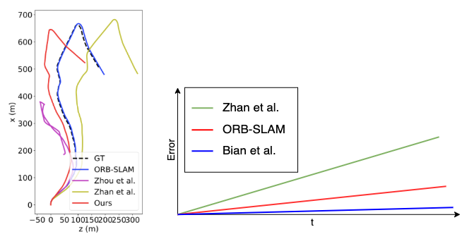
left image taken from “Unsupervised Scale-consistent Depth and Ego-motion Learning from Monocular Video”.
Therefore modelling the error of the state (i.e. error-state) is more likely that will be model correctly by a linear model. Therefore, we can avoid some noise coming from trying to model highly non-linear behaviour by modelling the error-state. Let’s define the error-state as (e=mu_t-mu_{t-1}). We can approximate (mathbf f(mu_{t-1})) using the Taylor series expansion only using the first derivative. Therefore (mathbf f(mu_{t-1}) approx mu_{t-1} + Fe_{t-1}). Replacing this and rearranging equation we end up with the final equations for the Error state — Extended Kalman Filter (ES-EKF)
Prediction step
[begin{align}
s_t &= mathbf f(s_{t-1},u)\
P_t &= FP_{t-1}F^T+BQB^T\
end{align}]
Update step:
[begin{align}K &= PH^T(HPH^T+R)^{-1}\
e_t &= K(z-h(mu_{t-1}))\
s_t &= s_{t-1} + e_t\
P_t &= (I+KH)P_{t-1}
end{align}]
Keep in mind that now we are tracking the error state and the covariance of the error, therefore we need to predict the state (s_t) and correct it by using the error-state during the update step, otherwise, we can estimate the state directly using (mathbf f(cdot)) as in ithe prediction step.
(if you see I have made a mistake, don’t hesitate to tell me).

The Kalman filter keeps track of the estimated state of the system and the variance or uncertainty of the estimate. The estimate is updated using a state transition model and measurements.  denotes the estimate of the system’s state at time step k before the k-th measurement yk has been taken into account;
  is the corresponding uncertainty.
For statistics and control theory, Kalman filtering, also known as linear quadratic estimation (LQE), is an algorithm that uses a series of measurements observed over time, including statistical noise and other inaccuracies, and produces estimates of unknown variables that tend to be more accurate than those based on a single measurement alone, by estimating a joint probability distribution over the variables for each timeframe. The filter is named after Rudolf E. Kálmán, who was one of the primary developers of its theory.
This digital filter is sometimes termed the Stratonovich–Kalman–Bucy filter because it is a special case of a more general, nonlinear filter developed somewhat earlier by the Soviet mathematician Ruslan Stratonovich.[1][2][3][4] In fact, some of the special case linear filter’s equations appeared in papers by Stratonovich that were published before summer 1960, when Kalman met with Stratonovich during a conference in Moscow.[5]
Kalman filtering[6] has numerous technological applications. A common application is for guidance, navigation, and control of vehicles, particularly aircraft, spacecraft and ships positioned dynamically.[7] Furthermore, Kalman filtering is a concept much applied in time series analysis used for topics such as signal processing and econometrics. Kalman filtering is also one of the main topics of robotic motion planning and control[8][9] and can be used for trajectory optimization.[10] Kalman filtering also works for modeling the central nervous system’s control of movement. Due to the time delay between issuing motor commands and receiving sensory feedback, the use of Kalman filters[11] provides a realistic model for making estimates of the current state of a motor system and issuing updated commands.[12]
The algorithm works by a two-phase process. For the prediction phase, the Kalman filter produces estimates of the current state variables, along with their uncertainties. Once the outcome of the next measurement (necessarily corrupted with some error, including random noise) is observed, these estimates are updated using a weighted average, with more weight being given to estimates with greater certainty. The algorithm is recursive. It can operate in real time, using only the present input measurements and the state calculated previously and its uncertainty matrix; no additional past information is required.
Optimality of Kalman filtering assumes that errors have a normal (Gaussian) distribution. In the words of Rudolf E. Kálmán: «In summary, the following assumptions are made about random processes: Physical random phenomena may be thought of as due to primary random sources exciting dynamic systems. The primary sources are assumed to be independent gaussian random processes with zero mean; the dynamic systems will be linear.»[13] Though regardless of Gaussianity, if the process and measurement covariances are known, the Kalman filter is the best possible linear estimator in the minimum mean-square-error sense.[14]
Extensions and generalizations of the method have also been developed, such as the extended Kalman filter and the unscented Kalman filter which work on nonlinear systems. The basis is a hidden Markov model such that the state space of the latent variables is continuous and all latent and observed variables have Gaussian distributions. Kalman filtering has been used successfully in multi-sensor fusion,[15] and distributed sensor networks to develop distributed or consensus Kalman filtering.[16]
History[edit]
The filtering method is named for Hungarian émigré Rudolf E. Kálmán, although Thorvald Nicolai Thiele[17][18] and Peter Swerling developed a similar algorithm earlier. Richard S. Bucy of the Johns Hopkins Applied Physics Laboratory contributed to the theory, causing it to be known sometimes as Kalman–Bucy filtering.
Stanley F. Schmidt is generally credited with developing the first implementation of a Kalman filter. He realized that the filter could be divided into two distinct parts, with one part for time periods between sensor outputs and another part for incorporating measurements.[19] It was during a visit by Kálmán to the NASA Ames Research Center that Schmidt saw the applicability of Kálmán’s ideas to the nonlinear problem of trajectory estimation for the Apollo program resulting in its incorporation in the Apollo navigation computer.[20]: 16
This Kalman filtering was first described and developed partially in technical papers by Swerling (1958), Kalman (1960) and Kalman and Bucy (1961).
The Apollo computer used 2k of magnetic core RAM and 36k wire rope […]. The CPU was built from ICs […]. Clock speed was under 100 kHz […]. The fact that the MIT engineers were able to pack such good software (one of the very first applications of the Kalman filter) into such a tiny computer is truly remarkable.
— Interview with Jack Crenshaw, by Matthew Reed, TRS-80.org (2009) [1]
Kalman filters have been vital in the implementation of the navigation systems of U.S. Navy nuclear ballistic missile submarines, and in the guidance and navigation systems of cruise missiles such as the U.S. Navy’s Tomahawk missile and the U.S. Air Force’s Air Launched Cruise Missile. They are also used in the guidance and navigation systems of reusable launch vehicles and the attitude control and navigation systems of spacecraft which dock at the International Space Station.[21]
Overview of the calculation[edit]
Kalman filtering uses a system’s dynamic model (e.g., physical laws of motion), known control inputs to that system, and multiple sequential measurements (such as from sensors) to form an estimate of the system’s varying quantities (its state) that is better than the estimate obtained by using only one measurement alone. As such, it is a common sensor fusion and data fusion algorithm.
Noisy sensor data, approximations in the equations that describe the system evolution, and external factors that are not accounted for, all limit how well it is possible to determine the system’s state. The Kalman filter deals effectively with the uncertainty due to noisy sensor data and, to some extent, with random external factors. The Kalman filter produces an estimate of the state of the system as an average of the system’s predicted state and of the new measurement using a weighted average. The purpose of the weights is that values with better (i.e., smaller) estimated uncertainty are «trusted» more. The weights are calculated from the covariance, a measure of the estimated uncertainty of the prediction of the system’s state. The result of the weighted average is a new state estimate that lies between the predicted and measured state, and has a better estimated uncertainty than either alone. This process is repeated at every time step, with the new estimate and its covariance informing the prediction used in the following iteration. This means that Kalman filter works recursively and requires only the last «best guess», rather than the entire history, of a system’s state to calculate a new state.
The measurements’ certainty-grading and current-state estimate are important considerations. It is common to discuss the filter’s response in terms of the Kalman filter’s gain. The Kalman-gain is the weight given to the measurements and current-state estimate, and can be «tuned» to achieve a particular performance. With a high gain, the filter places more weight on the most recent measurements, and thus conforms to them more responsively. With a low gain, the filter conforms to the model predictions more closely. At the extremes, a high gain close to one will result in a more jumpy estimated trajectory, while a low gain close to zero will smooth out noise but decrease the responsiveness.
When performing the actual calculations for the filter (as discussed below), the state estimate and covariances are coded into matrices because of the multiple dimensions involved in a single set of calculations. This allows for a representation of linear relationships between different state variables (such as position, velocity, and acceleration) in any of the transition models or covariances.
Example application[edit]
As an example application, consider the problem of determining the precise location of a truck. The truck can be equipped with a GPS unit that provides an estimate of the position within a few meters. The GPS estimate is likely to be noisy; readings ‘jump around’ rapidly, though remaining within a few meters of the real position. In addition, since the truck is expected to follow the laws of physics, its position can also be estimated by integrating its velocity over time, determined by keeping track of wheel revolutions and the angle of the steering wheel. This is a technique known as dead reckoning. Typically, the dead reckoning will provide a very smooth estimate of the truck’s position, but it will drift over time as small errors accumulate.
For this example, the Kalman filter can be thought of as operating in two distinct phases: predict and update. In the prediction phase, the truck’s old position will be modified according to the physical laws of motion (the dynamic or «state transition» model). Not only will a new position estimate be calculated, but also a new covariance will be calculated as well. Perhaps the covariance is proportional to the speed of the truck because we are more uncertain about the accuracy of the dead reckoning position estimate at high speeds but very certain about the position estimate at low speeds. Next, in the update phase, a measurement of the truck’s position is taken from the GPS unit. Along with this measurement comes some amount of uncertainty, and its covariance relative to that of the prediction from the previous phase determines how much the new measurement will affect the updated prediction. Ideally, as the dead reckoning estimates tend to drift away from the real position, the GPS measurement should pull the position estimate back toward the real position but not disturb it to the point of becoming noisy and rapidly jumping.
Technical description and context[edit]
The Kalman filter is an efficient recursive filter estimating the internal state of a linear dynamic system from a series of noisy measurements. It is used in a wide range of engineering and econometric applications from radar and computer vision to estimation of structural macroeconomic models,[22][23] and is an important topic in control theory and control systems engineering. Together with the linear-quadratic regulator (LQR), the Kalman filter solves the linear–quadratic–Gaussian control problem (LQG). The Kalman filter, the linear-quadratic regulator, and the linear–quadratic–Gaussian controller are solutions to what arguably are the most fundamental problems of control theory.
In most applications, the internal state is much larger (has more degrees of freedom) than the few «observable» parameters which are measured. However, by combining a series of measurements, the Kalman filter can estimate the entire internal state.
For the Dempster–Shafer theory, each state equation or observation is considered a special case of a linear belief function and the Kalman filtering is a special case of combining linear belief functions on a join-tree or Markov tree. Additional methods include belief filtering which use Bayes or evidential updates to the state equations.
A wide variety of Kalman filters exists by now, from Kalman’s original formulation — now termed the «simple» Kalman filter, the Kalman–Bucy filter, Schmidt’s «extended» filter, the information filter, and a variety of «square-root» filters that were developed by Bierman, Thornton, and many others. Perhaps the most commonly used type of very simple Kalman filter is the phase-locked loop, which is now ubiquitous in radios, especially frequency modulation (FM) radios, television sets, satellite communications receivers, outer space communications systems, and nearly any other electronic communications equipment.
Underlying dynamic system model[edit]
|
This section needs expansion. You can help by adding to it. (August 2011) |
Kalman filtering is based on linear dynamic systems discretized in the time domain. They are modeled on a Markov chain built on linear operators perturbed by errors that may include Gaussian noise. The state of the target system refers to the ground truth (yet hidden) system configuration of interest, which is represented as a vector of real numbers. At each discrete time increment, a linear operator is applied to the state to generate the new state, with some noise mixed in, and optionally some information from the controls on the system if they are known. Then, another linear operator mixed with more noise generates the measurable outputs (i.e., observation) from the true («hidden») state. The Kalman filter may be regarded as analogous to the hidden Markov model, with the difference that the hidden state variables have values in a continuous space as opposed to a discrete state space as for the hidden Markov model. There is a strong analogy between the equations of a Kalman Filter and those of the hidden Markov model. A review of this and other models is given in Roweis and Ghahramani (1999)[24] and Hamilton (1994), Chapter 13.[25]
In order to use the Kalman filter to estimate the internal state of a process given only a sequence of noisy observations, one must model the process in accordance with the following framework. This means specifying the matrices, for each time-step k, following:
- Fk, the state-transition model;
- Hk, the observation model;
- Qk, the covariance of the process noise;
- Rk, the covariance of the observation noise;
- and sometimes Bk, the control-input model as described below; if Bk is included, then there is also
- uk, the control vector, representing the controlling input into control-input model.
![]()
Model underlying the Kalman filter. Squares represent matrices. Ellipses represent multivariate normal distributions (with the mean and covariance matrix enclosed). Unenclosed values are vectors. For the simple case, the various matrices are constant with time, and thus the subscripts are not used, but Kalman filtering allows any of them to change each time step.
The Kalman filter model assumes the true state at time k is evolved from the state at (k − 1) according to

where
At time k an observation (or measurement) zk of the true state xk is made according to

where
- Hk is the observation model, which maps the true state space into the observed space and
- vk is the observation noise, which is assumed to be zero mean Gaussian white noise with covariance Rk:
 .
.

The initial state, and the noise vectors at each step {x0, w1, …, wk, v1, … ,vk} are all assumed to be mutually independent.
Many real-time dynamic systems do not exactly conform to this model. In fact, unmodeled dynamics can seriously degrade the filter performance, even when it was supposed to work with unknown stochastic signals as inputs. The reason for this is that the effect of unmodeled dynamics depends on the input, and, therefore, can bring the estimation algorithm to instability (it diverges). On the other hand, independent white noise signals will not make the algorithm diverge. The problem of distinguishing between measurement noise and unmodeled dynamics is a difficult one and is treated as a problem of control theory using robust control.[26][27]
Details[edit]
The Kalman filter is a recursive estimator. This means that only the estimated state from the previous time step and the current measurement are needed to compute the estimate for the current state. In contrast to batch estimation techniques, no history of observations and/or estimates is required. In what follows, the notation  represents the estimate of
  at time n given observations up to and including at time m ≤ n.
The state of the filter is represented by two variables:
The algorithm structure of the Kalman filter resembles that of Alpha beta filter. The Kalman filter can be written as a single equation; however, it is most often conceptualized as two distinct phases: «Predict» and «Update». The predict phase uses the state estimate from the previous timestep to produce an estimate of the state at the current timestep. This predicted state estimate is also known as the a priori state estimate because, although it is an estimate of the state at the current timestep, it does not include observation information from the current timestep. In the update phase, the innovation (the pre-fit residual), i.e. the difference between the current a priori prediction and the current observation information, is multiplied by the optimal Kalman gain and combined with the previous state estimate to refine the state estimate. This improved estimate based on the current observation is termed the a posteriori state estimate.
Typically, the two phases alternate, with the prediction advancing the state until the next scheduled observation, and the update incorporating the observation. However, this is not necessary; if an observation is unavailable for some reason, the update may be skipped and multiple prediction procedures performed. Likewise, if multiple independent observations are available at the same time, multiple update procedures may be performed (typically with different observation matrices Hk).[28][29]
Predict[edit]
Update[edit]
| Innovation or measurement pre-fit residual | 
|
| Innovation (or pre-fit residual) covariance | 
|
| Optimal Kalman gain | 
|
| Updated (a posteriori) state estimate | 
|
| Updated (a posteriori) estimate covariance | 
|
| Measurement post-fit residual | 
|
The formula for the updated (a posteriori) estimate covariance above is valid for the optimal Kk gain that minimizes the residual error, in which form it is most widely used in applications. Proof of the formulae is found in the derivations section, where the formula valid for any Kk is also shown.
A more intuitive way to express the updated state estimate ( ) is:
) is:

This expression reminds us of a linear interpolation,  for
for  between [0,1].
In our case:
This expression also resembles the alpha beta filter update step.
Invariants[edit]
If the model is accurate, and the values for  and
and  accurately reflect the distribution of the initial state values, then the following invariants are preserved:
![{displaystyle {begin{aligned}operatorname {E} [mathbf {x} _{k}-{hat {mathbf {x} }}_{kmid k}]&=operatorname {E} [mathbf {x} _{k}-{hat {mathbf {x} }}_{kmid k-1}]=0\operatorname {E} [{tilde {mathbf {y} }}_{k}]&=0end{aligned}}}](https://wikimedia.org/api/rest_v1/media/math/render/svg/b8f5d60c0c6af2a77e632b6b4140752357d1d908)
where ![{displaystyle operatorname {E} [xi ]}](https://wikimedia.org/api/rest_v1/media/math/render/svg/261957bffe5d89e65e9d27dfa34c5f86f6017baa) is the expected value of
is the expected value of  . That is, all estimates have a mean error of zero.
Also:

so covariance matrices accurately reflect the covariance of estimates.
Estimation of the noise covariances Qk and Rk[edit]
Practical implementation of a Kalman Filter is often difficult due to the difficulty of getting a good estimate of the noise covariance matrices Qk and Rk. Extensive research has been done to estimate these covariances from data. One practical method of doing this is the autocovariance least-squares (ALS) technique that uses the time-lagged autocovariances of routine operating data to estimate the covariances.[30][31] The GNU Octave and Matlab code used to calculate the noise covariance matrices using the ALS technique is available online using the GNU General Public License.[32] Field Kalman Filter (FKF), a Bayesian algorithm, which allows simultaneous estimation of the state, parameters and noise covariance has been proposed.[33] The FKF algorithm has a recursive formulation, good observed convergence, and relatively low complexity, thus suggesting that the FKF algorithm may possibly be a worthwhile alternative to the Autocovariance Least-Squares methods.
Optimality and performance[edit]
It follows from theory that the Kalman filter is the optimal linear filter in cases where a) the model matches the real system perfectly, b) the entering noise is «white» (uncorrelated) and c) the covariances of the noise are known exactly. Correlated noises can also be treated using Kalman filters.[34]
Several methods for the noise covariance estimation have been proposed during past decades, including ALS, mentioned in the section above. After the covariances are estimated, it is useful to evaluate the performance of the filter; i.e., whether it is possible to improve the state estimation quality. If the Kalman filter works optimally, the innovation sequence (the output prediction error) is a white noise, therefore the whiteness property of the innovations measures filter performance. Several different methods can be used for this purpose.[35] If the noise terms are distributed in a non-Gaussian manner, methods for assessing performance of the filter estimate, which use probability inequalities or large-sample theory, are known in the literature.[36][37]
Example application, technical[edit]

Truth;
filtered process;
observations.
Consider a truck on frictionless, straight rails. Initially, the truck is stationary at position 0, but it is buffeted this way and that by random uncontrolled forces. We measure the position of the truck every Δt seconds, but these measurements are imprecise; we want to maintain a model of the truck’s position and velocity. We show here how we derive the model from which we create our Kalman filter.
Since  are constant, their time indices are dropped.
The position and velocity of the truck are described by the linear state space

where  is the velocity, that is, the derivative of position with respect to time.
We assume that between the (k − 1) and k timestep, uncontrolled forces cause a constant acceleration of ak that is normally distributed with mean 0 and standard deviation σa. From Newton’s laws of motion we conclude that

(there is no  term since there are no known control inputs. Instead, ak is the effect of an unknown input and
  applies that effect to the state vector) where
![{displaystyle {begin{aligned}mathbf {F} &={begin{bmatrix}1&Delta t\0&1end{bmatrix}}\[4pt]mathbf {G} &={begin{bmatrix}{frac {1}{2}}{Delta t}^{2}\[6pt]Delta tend{bmatrix}}end{aligned}}}](https://wikimedia.org/api/rest_v1/media/math/render/svg/03f9aa60ead12f434f4197b8c91ddad8c1b08ac6)
so that

where
![{displaystyle {begin{aligned}mathbf {w} _{k}&sim N(0,mathbf {Q} )\mathbf {Q} &=mathbf {G} mathbf {G} ^{textsf {T}}sigma _{a}^{2}={begin{bmatrix}{frac {1}{4}}{Delta t}^{4}&{frac {1}{2}}{Delta t}^{3}\[6pt]{frac {1}{2}}{Delta t}^{3}&{Delta t}^{2}end{bmatrix}}sigma _{a}^{2}.end{aligned}}}](https://wikimedia.org/api/rest_v1/media/math/render/svg/2ec09cb336ca77b3ef6203ebc27d13a302cf62cc)
The matrix  is not full rank (it is of rank one if
  ). Hence, the distribution
  is not absolutely continuous and has no probability density function. Another way to express this, avoiding explicit degenerate distributions is given by

At each time phase, a noisy measurement of the true position of the truck is made. Let us suppose the measurement noise vk is also distributed normally, with mean 0 and standard deviation σz.

where

and
![{displaystyle mathbf {R} =mathrm {E} left[mathbf {v} _{k}mathbf {v} _{k}^{textsf {T}}right]={begin{bmatrix}sigma _{z}^{2}end{bmatrix}}}](https://wikimedia.org/api/rest_v1/media/math/render/svg/dbbc9b31d008d00147cf59b62a0a92d78297ca0b)
We know the initial starting state of the truck with perfect precision, so we initialize

and to tell the filter that we know the exact position and velocity, we give it a zero covariance matrix:

If the initial position and velocity are not known perfectly, the covariance matrix should be initialized with suitable variances on its diagonal:

The filter will then prefer the information from the first measurements over the information already in the model.
Asymptotic form[edit]
For simplicity, assume that the control input  . Then the Kalman filter may be written:
![{displaystyle {hat {mathbf {x} }}_{kmid k}=mathbf {F} _{k}{hat {mathbf {x} }}_{k-1mid k-1}+mathbf {K} _{k}[mathbf {z} _{k}-mathbf {H} _{k}mathbf {F} _{k}{hat {mathbf {x} }}_{k-1mid k-1}].}](https://wikimedia.org/api/rest_v1/media/math/render/svg/0fcfb5a306bbf523000da1394518cf482488fd1d)
A similar equation holds if we include a non-zero control input. Gain matrices  evolve independently of the measurements
  . From above, the four equations needed for updating the Kalman gain are as follows:

Since the gain matrices depend only on the model, and not the measurements, they may be computed offline. Convergence of the gain matrices to an asymptotic matrix  applies for conditions established in Walrand and Dimakis.[38] Simulations establish the number of steps to convergence. For the moving truck example described above, with
  . and
. and  , simulation shows convergence in
  iterations.
Using the asymptotic gain, and assuming  and
and  are independent of
  , the Kalman filter becomes a linear time-invariant filter:
![{displaystyle {hat {mathbf {x} }}_{k}=mathbf {F} {hat {mathbf {x} }}_{k-1}+mathbf {K} _{infty }[mathbf {z} _{k}-mathbf {H} mathbf {F} {hat {mathbf {x} }}_{k-1}].}](https://wikimedia.org/api/rest_v1/media/math/render/svg/76b977e658b713bf9847f509957c98319d73cacb)
The asymptotic gain , if it exists, can be computed by first solving the following discrete Riccati equation for the asymptotic state covariance  :[38]
:[38]

The asymptotic gain is then computed as before.

Additionally, a form of the asymptotic Kalman filter more commonly used in control theory is given by
![{displaystyle {displaystyle {hat {mathbf {x} }}_{k+1}=mathbf {F} {hat {mathbf {x} }}_{k}+mathbf {B} mathbf {u} _{k}+mathbf {overline {K}} _{infty }[mathbf {z} _{k}-mathbf {H} {hat {mathbf {x} }}_{k}],}}](https://wikimedia.org/api/rest_v1/media/math/render/svg/bd519bc83300a8923c8aec3bbdd8664daed84bbe)
where

This leads to an estimator of the form

Derivations[edit]
The Kalman filter can be derived as a generalized least squares method operating on previous data.[39]
Deriving the posteriori estimate covariance matrix[edit]
Starting with our invariant on the error covariance Pk | k as above

substitute in the definition of
![{displaystyle mathbf {P} _{kmid k}=operatorname {cov} left[mathbf {x} _{k}-left({hat {mathbf {x} }}_{kmid k-1}+mathbf {K} _{k}{tilde {mathbf {y} }}_{k}right)right]}](https://wikimedia.org/api/rest_v1/media/math/render/svg/b31ed7985490d3d6803ac08a7965ad1b250c4554)
and substitute 
![{displaystyle mathbf {P} _{kmid k}=operatorname {cov} left(mathbf {x} _{k}-left[{hat {mathbf {x} }}_{kmid k-1}+mathbf {K} _{k}left(mathbf {z} _{k}-mathbf {H} _{k}{hat {mathbf {x} }}_{kmid k-1}right)right]right)}](https://wikimedia.org/api/rest_v1/media/math/render/svg/3fc500651c69cafbe9f07a93541cb3166d787126)
and
![{displaystyle mathbf {P} _{kmid k}=operatorname {cov} left(mathbf {x} _{k}-left[{hat {mathbf {x} }}_{kmid k-1}+mathbf {K} _{k}left(mathbf {H} _{k}mathbf {x} _{k}+mathbf {v} _{k}-mathbf {H} _{k}{hat {mathbf {x} }}_{kmid k-1}right)right]right)}](https://wikimedia.org/api/rest_v1/media/math/render/svg/5f9076bf807d7ed72fbd6246635cf2b7da91ee7c)
and by collecting the error vectors we get
![{displaystyle mathbf {P} _{kmid k}=operatorname {cov} left[left(mathbf {I} -mathbf {K} _{k}mathbf {H} _{k}right)left(mathbf {x} _{k}-{hat {mathbf {x} }}_{kmid k-1}right)-mathbf {K} _{k}mathbf {v} _{k}right]}](https://wikimedia.org/api/rest_v1/media/math/render/svg/1df4494c4e4fbff6fccdac6368485af96dac9b82)
Since the measurement error vk is uncorrelated with the other terms, this becomes
![{displaystyle mathbf {P} _{kmid k}=operatorname {cov} left[left(mathbf {I} -mathbf {K} _{k}mathbf {H} _{k}right)left(mathbf {x} _{k}-{hat {mathbf {x} }}_{kmid k-1}right)right]+operatorname {cov} left[mathbf {K} _{k}mathbf {v} _{k}right]}](https://wikimedia.org/api/rest_v1/media/math/render/svg/4591ba7c762680cfc0eb090f2c358df87b4d1e4c)
by the properties of vector covariance this becomes

which, using our invariant on Pk | k−1 and the definition of Rk becomes

This formula (sometimes known as the Joseph form of the covariance update equation) is valid for any value of Kk. It turns out that if Kk is the optimal Kalman gain, this can be simplified further as shown below.
Kalman gain derivation[edit]
The Kalman filter is a minimum mean-square error estimator. The error in the a posteriori state estimation is

We seek to minimize the expected value of the square of the magnitude of this vector, ![{displaystyle operatorname {E} left[left|mathbf {x} _{k}-{hat {mathbf {x} }}_{k|k}right|^{2}right]}](https://wikimedia.org/api/rest_v1/media/math/render/svg/9980afd591249f61711d6020cb30a0bcd54ec641) . This is equivalent to minimizing the trace of the a posteriori estimate covariance matrix
. This is equivalent to minimizing the trace of the a posteriori estimate covariance matrix  . By expanding out the terms in the equation above and collecting, we get:
![{displaystyle {begin{aligned}mathbf {P} _{kmid k}&=mathbf {P} _{kmid k-1}-mathbf {K} _{k}mathbf {H} _{k}mathbf {P} _{kmid k-1}-mathbf {P} _{kmid k-1}mathbf {H} _{k}^{textsf {T}}mathbf {K} _{k}^{textsf {T}}+mathbf {K} _{k}left(mathbf {H} _{k}mathbf {P} _{kmid k-1}mathbf {H} _{k}^{textsf {T}}+mathbf {R} _{k}right)mathbf {K} _{k}^{textsf {T}}\[6pt]&=mathbf {P} _{kmid k-1}-mathbf {K} _{k}mathbf {H} _{k}mathbf {P} _{kmid k-1}-mathbf {P} _{kmid k-1}mathbf {H} _{k}^{textsf {T}}mathbf {K} _{k}^{textsf {T}}+mathbf {K} _{k}mathbf {S} _{k}mathbf {K} _{k}^{textsf {T}}end{aligned}}}](https://wikimedia.org/api/rest_v1/media/math/render/svg/be6f9e0fc4bee39b78b2b9d62ecafaf0954143af)
The trace is minimized when its matrix derivative with respect to the gain matrix is zero. Using the gradient matrix rules and the symmetry of the matrices involved we find that

Solving this for Kk yields the Kalman gain:

This gain, which is known as the optimal Kalman gain, is the one that yields MMSE estimates when used.
Simplification of the posteriori error covariance formula[edit]
The formula used to calculate the a posteriori error covariance can be simplified when the Kalman gain equals the optimal value derived above. Multiplying both sides of our Kalman gain formula on the right by SkKkT, it follows that

Referring back to our expanded formula for the a posteriori error covariance,

we find the last two terms cancel out, giving

This formula is computationally cheaper and thus nearly always used in practice, but is only correct for the optimal gain. If arithmetic precision is unusually low causing problems with numerical stability, or if a non-optimal Kalman gain is deliberately used, this simplification cannot be applied; the a posteriori error covariance formula as derived above (Joseph form) must be used.
Sensitivity analysis[edit]
The Kalman filtering equations provide an estimate of the state and its error covariance  recursively. The estimate and its quality depend on the system parameters and the noise statistics fed as inputs to the estimator. This section analyzes the effect of uncertainties in the statistical inputs to the filter.[40] In the absence of reliable statistics or the true values of noise covariance matrices
  and
and  , the expression
no longer provides the actual error covariance. In other words, ![{displaystyle mathbf {P} _{kmid k}neq Eleft[left(mathbf {x} _{k}-{hat {mathbf {x} }}_{kmid k}right)left(mathbf {x} _{k}-{hat {mathbf {x} }}_{kmid k}right)^{textsf {T}}right]}](https://wikimedia.org/api/rest_v1/media/math/render/svg/14f468d3696299953a87882fe8987d019be46f87) . In most real-time applications, the covariance matrices that are used in designing the Kalman filter are different from the actual (true) noise covariances matrices.[citation needed] This sensitivity analysis describes the behavior of the estimation error covariance when the noise covariances as well as the system matrices and that are fed as inputs to the filter are incorrect. Thus, the sensitivity analysis describes the robustness (or sensitivity) of the estimator to misspecified statistical and parametric inputs to the estimator.
. In most real-time applications, the covariance matrices that are used in designing the Kalman filter are different from the actual (true) noise covariances matrices.[citation needed] This sensitivity analysis describes the behavior of the estimation error covariance when the noise covariances as well as the system matrices and that are fed as inputs to the filter are incorrect. Thus, the sensitivity analysis describes the robustness (or sensitivity) of the estimator to misspecified statistical and parametric inputs to the estimator.
This discussion is limited to the error sensitivity analysis for the case of statistical uncertainties. Here the actual noise covariances are denoted by  and
and  respectively, whereas the design values used in the estimator are and respectively. The actual error covariance is denoted by
  and as computed by the Kalman filter is referred to as the Riccati variable. When
  and
and  , this means that
  . While computing the actual error covariance using
 ![{displaystyle mathbf {P} _{kmid k}^{a}=Eleft[left(mathbf {x} _{k}-{hat {mathbf {x} }}_{kmid k}right)left(mathbf {x} _{k}-{hat {mathbf {x} }}_{kmid k}right)^{textsf {T}}right]}](https://wikimedia.org/api/rest_v1/media/math/render/svg/b8bfa69cc3749d0b62c6d50dc98080b54b24ea12) , substituting for Failed to parse (SVG (MathML can be enabled via browser plugin): Invalid response («Math extension cannot connect to Restbase.») from server «/mathoid/local/v1/»:): {displaystyle widehat{mathbf{x}}_{k mid k}}
, substituting for Failed to parse (SVG (MathML can be enabled via browser plugin): Invalid response («Math extension cannot connect to Restbase.») from server «/mathoid/local/v1/»:): {displaystyle widehat{mathbf{x}}_{k mid k}}
and using the fact that ![{displaystyle Eleft[mathbf {w} _{k}mathbf {w} _{k}^{textsf {T}}right]=mathbf {Q} _{k}^{a}}](https://wikimedia.org/api/rest_v1/media/math/render/svg/d683b5e826696f9302ad471107d89cbd574a2861) and
and ![{displaystyle Eleft[mathbf {v} _{k}mathbf {v} _{k}^{textsf {T}}right]=mathbf {R} _{k}^{a}}](https://wikimedia.org/api/rest_v1/media/math/render/svg/d89dca74f5288b67fbe0fa2855a370545ddb4006) , results in the following recursive equations for :
, results in the following recursive equations for :

and

While computing , by design the filter implicitly assumes that ![{displaystyle Eleft[mathbf {w} _{k}mathbf {w} _{k}^{textsf {T}}right]=mathbf {Q} _{k}}](https://wikimedia.org/api/rest_v1/media/math/render/svg/3e913b662d3d03c3b59ce4a86767ae6c4a57c311) and
and ![{displaystyle Eleft[mathbf {v} _{k}mathbf {v} _{k}^{textsf {T}}right]=mathbf {R} _{k}}](https://wikimedia.org/api/rest_v1/media/math/render/svg/819ee3b84d0b2613dc716ed09927696fda25baf5) . The recursive expressions for and are identical except for the presence of and in place of the design values and respectively. Researches have been done to analyze Kalman filter system’s robustness.[41]
. The recursive expressions for and are identical except for the presence of and in place of the design values and respectively. Researches have been done to analyze Kalman filter system’s robustness.[41]
Square root form[edit]
One problem with the Kalman filter is its numerical stability. If the process noise covariance Qk is small, round-off error often causes a small positive eigenvalue to be computed as a negative number. This renders the numerical representation of the state covariance matrix P indefinite, while its true form is positive-definite.
Positive definite matrices have the property that they have a triangular matrix square root P = S·ST. This can be computed efficiently using the Cholesky factorization algorithm, but more importantly, if the covariance is kept in this form, it can never have a negative diagonal or become asymmetric. An equivalent form, which avoids many of the square root operations required by the matrix square root yet preserves the desirable numerical properties, is the U-D decomposition form, P = U·D·UT, where U is a unit triangular matrix (with unit diagonal), and D is a diagonal matrix.
Between the two, the U-D factorization uses the same amount of storage, and somewhat less computation, and is the most commonly used square root form. (Early literature on the relative efficiency is somewhat misleading, as it assumed that square roots were much more time-consuming than divisions,[42]: 69 while on 21st-century computers they are only slightly more expensive.)
Efficient algorithms for the Kalman prediction and update steps in the square root form were developed by G. J. Bierman and C. L. Thornton.[42][43]
The L·D·LT decomposition of the innovation covariance matrix Sk is the basis for another type of numerically efficient and robust square root filter.[44] The algorithm starts with the LU decomposition as implemented in the Linear Algebra PACKage (LAPACK). These results are further factored into the L·D·LT structure with methods given by Golub and Van Loan (algorithm 4.1.2) for a symmetric nonsingular matrix.[45] Any singular covariance matrix is pivoted so that the first diagonal partition is nonsingular and well-conditioned. The pivoting algorithm must retain any portion of the innovation covariance matrix directly corresponding to observed state-variables Hk·xk|k-1 that are associated with auxiliary observations in
yk. The l·d·lt square-root filter requires orthogonalization of the observation vector.[43][44] This may be done with the inverse square-root of the covariance matrix for the auxiliary variables using Method 2 in Higham (2002, p. 263).[46]
Parallel form[edit]
The Kalman filter is efficient for sequential data processing on central processing units (CPUs), but in its original form it is inefficient on parallel architectures such as graphics processing units (GPUs). It is however possible to express the filter-update routine in terms of an associative operator using the formulation in Särkkä (2021).[47] The filter solution can then be retrieved by the use of a prefix sum algorithm which can be efficiently implemented on GPU.[48] This reduces the computational complexity from  in the number of time steps to
  .
.
Relationship to recursive Bayesian estimation[edit]
The Kalman filter can be presented as one of the simplest dynamic Bayesian networks. The Kalman filter calculates estimates of the true values of states recursively over time using incoming measurements and a mathematical process model. Similarly, recursive Bayesian estimation calculates estimates of an unknown probability density function (PDF) recursively over time using incoming measurements and a mathematical process model.[49]
In recursive Bayesian estimation, the true state is assumed to be an unobserved Markov process, and the measurements are the observed states of a hidden Markov model (HMM).

Because of the Markov assumption, the true state is conditionally independent of all earlier states given the immediately previous state.

Similarly, the measurement at the k-th timestep is dependent only upon the current state and is conditionally independent of all other states given the current state.

Using these assumptions the probability distribution over all states of the hidden Markov model can be written simply as:

However, when a Kalman filter is used to estimate the state x, the probability distribution of interest is that associated with the current states conditioned on the measurements up to the current timestep. This is achieved by marginalizing out the previous states and dividing by the probability of the measurement set.
This results in the predict and update phases of the Kalman filter written probabilistically. The probability distribution associated with the predicted state is the sum (integral) of the products of the probability distribution associated with the transition from the (k − 1)-th timestep to the k-th and the probability distribution associated with the previous state, over all possible  .
.

The measurement set up to time t is

The probability distribution of the update is proportional to the product of the measurement likelihood and the predicted state.

The denominator

is a normalization term.
The remaining probability density functions are

The PDF at the previous timestep is assumed inductively to be the estimated state and covariance. This is justified because, as an optimal estimator, the Kalman filter makes best use of the measurements, therefore the PDF for  given the measurements
  is the Kalman filter estimate.
Marginal likelihood[edit]
Related to the recursive Bayesian interpretation described above, the Kalman filter can be viewed as a generative model, i.e., a process for generating a stream of random observations z = (z0, z1, z2, …). Specifically, the process is
- Sample a hidden state from the Gaussian prior distribution .
- Sample an observation from the observation model .
- For , do
- Sample the next hidden state from the transition model
- Sample an observation from the observation model
- Sample the next hidden state


This process has identical structure to the hidden Markov model, except that the discrete state and observations are replaced with continuous variables sampled from Gaussian distributions.
In some applications, it is useful to compute the probability that a Kalman filter with a given set of parameters (prior distribution, transition and observation models, and control inputs) would generate a particular observed signal. This probability is known as the marginal likelihood because it integrates over («marginalizes out») the values of the hidden state variables, so it can be computed using only the observed signal. The marginal likelihood can be useful to evaluate different parameter choices, or to compare the Kalman filter against other models using Bayesian model comparison.
It is straightforward to compute the marginal likelihood as a side effect of the recursive filtering computation. By the chain rule, the likelihood can be factored as the product of the probability of each observation given previous observations,
- ,

and because the Kalman filter describes a Markov process, all relevant information from previous observations is contained in the current state estimate  Thus the marginal likelihood is given by

i.e., a product of Gaussian densities, each corresponding to the density of one observation zk under the current filtering distribution  . This can easily be computed as a simple recursive update; however, to avoid numeric underflow, in a practical implementation it is usually desirable to compute the log marginal likelihood
  instead. Adopting the convention
  , this can be done via the recursive update rule

where  is the dimension of the measurement vector.[50]
An important application where such a (log) likelihood of the observations (given the filter parameters) is used is multi-target tracking. For example, consider an object tracking scenario where a stream of observations is the input, however, it is unknown how many objects are in the scene (or, the number of objects is known but is greater than one). For such a scenario, it can be unknown apriori which observations/measurements were generated by which object. A multiple hypothesis tracker (MHT) typically will form different track association hypotheses, where each hypothesis can be considered as a Kalman filter (for the linear Gaussian case) with a specific set of parameters associated with the hypothesized object. Thus, it is important to compute the likelihood of the observations for the different hypotheses under consideration, such that the most-likely one can be found.
Information filter[edit]
In the information filter, or inverse covariance filter, the estimated covariance and estimated state are replaced by the information matrix and information vector respectively. These are defined as:

Similarly the predicted covariance and state have equivalent information forms, defined as:

as have the measurement covariance and measurement vector, which are defined as:

The information update now becomes a trivial sum.[51]

The main advantage of the information filter is that N measurements can be filtered at each time step simply by summing their information matrices and vectors.

To predict the information filter the information matrix and vector can be converted back to their state space equivalents, or alternatively the information space prediction can be used.[51]
![{displaystyle {begin{aligned}mathbf {M} _{k}&=left[mathbf {F} _{k}^{-1}right]^{textsf {T}}mathbf {Y} _{k-1mid k-1}mathbf {F} _{k}^{-1}\mathbf {C} _{k}&=mathbf {M} _{k}left[mathbf {M} _{k}+mathbf {Q} _{k}^{-1}right]^{-1}\mathbf {L} _{k}&=mathbf {I} -mathbf {C} _{k}\mathbf {Y} _{kmid k-1}&=mathbf {L} _{k}mathbf {M} _{k}mathbf {L} _{k}^{textsf {T}}+mathbf {C} _{k}mathbf {Q} _{k}^{-1}mathbf {C} _{k}^{textsf {T}}\{hat {mathbf {y} }}_{kmid k-1}&=mathbf {L} _{k}left[mathbf {F} _{k}^{-1}right]^{textsf {T}}{hat {mathbf {y} }}_{k-1mid k-1}end{aligned}}}](https://wikimedia.org/api/rest_v1/media/math/render/svg/160c07d9b85fcb57249512dc02c8c657e0bb986c)
Fixed-lag smoother[edit]
The optimal fixed-lag smoother provides the optimal estimate of  for a given fixed-lag
  using the measurements from
  to .[52] It can be derived using the previous theory via an augmented state, and the main equation of the filter is the following:

where:
- and
- where and are the prediction error covariance and the gains of the standard Kalman filter (i.e., ).
![{displaystyle mathbf {P} ^{(i)}=mathbf {P} left[left(mathbf {F} -mathbf {K} mathbf {H} right)^{textsf {T}}right]^{i}}](https://wikimedia.org/api/rest_v1/media/math/render/svg/d3f062727421b3b0781655e42ca094d1d950fb93)


If the estimation error covariance is defined so that
![{displaystyle mathbf {P} _{i}:=Eleft[left(mathbf {x} _{t-i}-{hat {mathbf {x} }}_{t-imid t}right)^{*}left(mathbf {x} _{t-i}-{hat {mathbf {x} }}_{t-imid t}right)mid z_{1}ldots z_{t}right],}](https://wikimedia.org/api/rest_v1/media/math/render/svg/8780d91a9b0e63eced8dd27ec2f8ed0b45c1de89)
then we have that the improvement on the estimation of  is given by:
![{displaystyle mathbf {P} -mathbf {P} _{i}=sum _{j=0}^{i}left[mathbf {P} ^{(j)}mathbf {H} ^{textsf {T}}left(mathbf {H} mathbf {P} mathbf {H} ^{textsf {T}}+mathbf {R} right)^{-1}mathbf {H} left(mathbf {P} ^{(i)}right)^{textsf {T}}right]}](https://wikimedia.org/api/rest_v1/media/math/render/svg/b0f8a12ef0ba8f26d287adc97353160f6cb9af36)
Fixed-interval smoothers[edit]
The optimal fixed-interval smoother provides the optimal estimate of  (
( ) using the measurements from a fixed interval to
  . This is also called «Kalman Smoothing». There are several smoothing algorithms in common use.
Rauch–Tung–Striebel[edit]
The Rauch–Tung–Striebel (RTS) smoother is an efficient two-pass algorithm for fixed interval smoothing.[53]
The forward pass is the same as the regular Kalman filter algorithm. These filtered a-priori and a-posteriori state estimates  , and covariances
  , are saved for use in the backward pass (for retrodiction).
In the backward pass, we compute the smoothed state estimates and covariances  . We start at the last time step and proceed backward in time using the following recursive equations:

where

 is the a-posteriori state estimate of timestep and
  is the a-priori state estimate of timestep
  . The same notation applies to the covariance.
Modified Bryson–Frazier smoother[edit]
An alternative to the RTS algorithm is the modified Bryson–Frazier (MBF) fixed interval smoother developed by Bierman.[43] This also uses a backward pass that processes data saved from the Kalman filter forward pass. The equations for the backward pass involve the recursive
computation of data which are used at each observation time to compute the smoothed state and covariance.
The recursive equations are

where  is the residual covariance and
  . The smoothed state and covariance can then be found by substitution in the equations

or

An important advantage of the MBF is that it does not require finding the inverse of the covariance matrix.
Minimum-variance smoother[edit]
The minimum-variance smoother can attain the best-possible error performance, provided that the models are linear, their parameters and the noise statistics are known precisely.[54] This smoother is a time-varying state-space generalization of the optimal non-causal Wiener filter.
The smoother calculations are done in two passes. The forward calculations involve a one-step-ahead predictor and are given by

The above system is known as the inverse Wiener-Hopf factor. The backward recursion is the adjoint of the above forward system. The result of the backward pass  may be calculated by operating the forward equations on the time-reversed
  and time reversing the result. In the case of output estimation, the smoothed estimate is given by

Taking the causal part of this minimum-variance smoother yields

which is identical to the minimum-variance Kalman filter. The above solutions minimize the variance of the output estimation error. Note that the Rauch–Tung–Striebel smoother derivation assumes that the underlying distributions are Gaussian, whereas the minimum-variance solutions do not. Optimal smoothers for state estimation and input estimation can be constructed similarly.
A continuous-time version of the above smoother is described in.[55][56]
Expectation–maximization algorithms may be employed to calculate approximate maximum likelihood estimates of unknown state-space parameters within minimum-variance filters and smoothers. Often uncertainties remain within problem assumptions. A smoother that accommodates uncertainties can be designed by adding a positive definite term to the Riccati equation.[57]
In cases where the models are nonlinear, step-wise linearizations may be within the minimum-variance filter and smoother recursions (extended Kalman filtering).
Frequency-weighted Kalman filters[edit]
Pioneering research on the perception of sounds at different frequencies was conducted by Fletcher and Munson in the 1930s. Their work led to a standard way of weighting measured sound levels within investigations of industrial noise and hearing loss. Frequency weightings have since been used within filter and controller designs to manage performance within bands of interest.
Typically, a frequency shaping function is used to weight the average power of the error spectral density in a specified frequency band. Let  denote the output estimation error exhibited by a conventional Kalman filter. Also, let
  denote a causal frequency weighting transfer function. The optimum solution which minimizes the variance of
  arises by simply constructing
  .
.
The design of remains an open question. One way of proceeding is to identify a system which generates the estimation error and setting equal to the inverse of that system.[58] This procedure may be iterated to obtain mean-square error improvement at the cost of increased filter order. The same technique can be applied to smoothers.
Nonlinear filters[edit]
The basic Kalman filter is limited to a linear assumption. More complex systems, however, can be nonlinear. The nonlinearity can be associated either with the process model or with the observation model or with both.
The most common variants of Kalman filters for non-linear systems are the Extended Kalman Filter and Unscented Kalman filter. The suitability of which filter to use depends on the non-linearity indices of the process and observation model.[59]
Extended Kalman filter[edit]
In the extended Kalman filter (EKF), the state transition and observation models need not be linear functions of the state but may instead be nonlinear functions. These functions are of differentiable type.

The function f can be used to compute the predicted state from the previous estimate and similarly the function h can be used to compute the predicted measurement from the predicted state. However, f and h cannot be applied to the covariance directly. Instead a matrix of partial derivatives (the Jacobian) is computed.
At each timestep the Jacobian is evaluated with current predicted states. These matrices can be used in the Kalman filter equations. This process essentially linearizes the nonlinear function around the current estimate.
Unscented Kalman filter[edit]
When the state transition and observation models—that is, the predict and update functions  and
and  —are highly nonlinear, the extended Kalman filter can give particularly poor performance.[60] This is because the covariance is propagated through linearization of the underlying nonlinear model. The unscented Kalman filter (UKF) [60] uses a deterministic sampling technique known as the unscented transformation (UT) to pick a minimal set of sample points (called sigma points) around the mean. The sigma points are then propagated through the nonlinear functions, from which a new mean and covariance estimate are then formed. The resulting filter depends on how the transformed statistics of the UT are calculated and which set of sigma points are used. It should be remarked that it is always possible to construct new UKFs in a consistent way.[61] For certain systems, the resulting UKF more accurately estimates the true mean and covariance.[62] This can be verified with Monte Carlo sampling or Taylor series expansion of the posterior statistics. In addition, this technique removes the requirement to explicitly calculate Jacobians, which for complex functions can be a difficult task in itself (i.e., requiring complicated derivatives if done analytically or being computationally costly if done numerically), if not impossible (if those functions are not differentiable).
Sigma points[edit]
For a random vector  , sigma points are any set of vectors

attributed with
- first-order weights that fulfill

- for all :


![{displaystyle E[x_{i}]=sum _{j=0}^{N}W_{j}^{a}s_{j,i}}](https://wikimedia.org/api/rest_v1/media/math/render/svg/675007e4cd61311f7ca86cfa1e7182c2a18d2fa1)
- second-order weights that fulfill

- for all pairs .

![{displaystyle (i,l)in {1,dots ,L}^{2}:E[x_{i}x_{l}]=sum _{j=0}^{N}W_{j}^{c}s_{j,i}s_{j,l}}](https://wikimedia.org/api/rest_v1/media/math/render/svg/4568b4d145d78fcd8e7e109df907af1021ef13cd)
A simple choice of sigma points and weights for  in the UKF algorithm is

where  is the mean estimate of . The vector
  is the jth column of
  where
where  . Typically, is obtained via Cholesky decomposition of
  . With some care the filter equations can be expressed in such a way that is evaluated directly without intermediate calculations of . This is referred to as the square-root unscented Kalman filter.[63]
The weight of the mean value,  , can be chosen arbitrarily.
Another popular parameterization (which generalizes the above) is

 and
and  control the spread of the sigma points.
  is related to the distribution of
  .
.
Appropriate values depend on the problem at hand, but a typical recommendation is  ,
,  , and
, and  . However, a larger value of (e.g.,
  ) may be beneficial in order to better capture the spread of the distribution and possible nonlinearities.[64] If the true distribution of is Gaussian, is optimal.[65]
Predict[edit]
As with the EKF, the UKF prediction can be used independently from the UKF update, in combination with a linear (or indeed EKF) update, or vice versa.
Given estimates of the mean and covariance, and , one obtains  sigma points as described in the section above. The sigma points are propagated through the transition function f.
- .

The propagated sigma points are weighed to produce the predicted mean and covariance.

where  are the first-order weights of the original sigma points, and
  are the second-order weights. The matrix is the covariance of the transition noise,
  .
.
Update[edit]
Given prediction estimates and , a new set of sigma points  with corresponding first-order weights
  and second-order weights
  is calculated.[66] These sigma points are transformed through the measurement function .
- .

Then the empirical mean and covariance of the transformed points are calculated.
![{displaystyle {begin{aligned}{hat {mathbf {z} }}&=sum _{j=0}^{2L}W_{j}^{a}mathbf {z} _{j}\[6pt]{hat {mathbf {S} }}_{k}&=sum _{j=0}^{2L}W_{j}^{c}(mathbf {z} _{j}-{hat {mathbf {z} }})(mathbf {z} _{j}-{hat {mathbf {z} }})^{textsf {T}}+mathbf {R} _{k}end{aligned}}}](https://wikimedia.org/api/rest_v1/media/math/render/svg/b4cbfafad41274db6e909b41006299ad5ba6400c)
where is the covariance matrix of the observation noise,  . Additionally, the cross covariance matrix is also needed

The Kalman gain is

The updated mean and covariance estimates are

Discriminative Kalman filter[edit]
When the observation model  is highly non-linear and/or non-Gaussian, it may prove advantageous to apply Bayes’ rule and estimate

where  for nonlinear functions
  . This replaces the generative specification of the standard Kalman filter with a discriminative model for the latent states given observations.
Under a stationary state model

where  , if
, if

then given a new observation , it follows that[67]

where

Note that this approximation requires  to be positive-definite; in the case that it is not,

is used instead. Such an approach proves particularly useful when the dimensionality of the observations is much greater than that of the latent states[68] and can be used build filters that are particularly robust to nonstationarities in the observation model.[69]
Adaptive Kalman filter[edit]
Adaptive Kalman filters allow to adapt for process dynamics which are not modeled in the process model  , which happens for example in the context of a maneuvering target when a constant velocity (reduced order) Kalman filter is employed for tracking.[70]
Kalman–Bucy filter[edit]
Kalman–Bucy filtering (named for Richard Snowden Bucy) is a continuous time version of Kalman filtering.[71][72]
It is based on the state space model

where  and
and  represent the intensities (or, more accurately: the Power Spectral Density — PSD — matrices) of the two white noise terms
  and
and  , respectively.
The filter consists of two differential equations, one for the state estimate and one for the covariance:

where the Kalman gain is given by

Note that in this expression for  the covariance of the observation noise represents at the same time the covariance of the prediction error (or innovation)
  ; these covariances are equal only in the case of continuous time.[73]
The distinction between the prediction and update steps of discrete-time Kalman filtering does not exist in continuous time.
The second differential equation, for the covariance, is an example of a Riccati equation. Nonlinear generalizations to Kalman–Bucy filters include continuous time extended Kalman filter.
Hybrid Kalman filter[edit]
Most physical systems are represented as continuous-time models while discrete-time measurements are made frequently for state estimation via a digital processor. Therefore, the system model and measurement model are given by

where
- .

Initialize[edit]
![{displaystyle {hat {mathbf {x} }}_{0mid 0}=Eleft[mathbf {x} (t_{0})right],mathbf {P} _{0mid 0}=operatorname {Var} left[mathbf {x} left(t_{0}right)right]}](https://wikimedia.org/api/rest_v1/media/math/render/svg/22f8d1d2c5bc4283dd4032d5de0b9dff4da51f0d)
Predict[edit]

The prediction equations are derived from those of continuous-time Kalman filter without update from measurements, i.e.,  . The predicted state and covariance are calculated respectively by solving a set of differential equations with the initial value equal to the estimate at the previous step.
For the case of linear time invariant systems, the continuous time dynamics can be exactly discretized into a discrete time system using matrix exponentials.
Update[edit]

The update equations are identical to those of the discrete-time Kalman filter.
Variants for the recovery of sparse signals[edit]
The traditional Kalman filter has also been employed for the recovery of sparse, possibly dynamic, signals from noisy observations. Recent works[74][75][76] utilize notions from the theory of compressed sensing/sampling, such as the restricted isometry property and related probabilistic recovery arguments, for sequentially estimating the sparse state in intrinsically low-dimensional systems.
Relation to Gaussian processes[edit]
Since linear Gaussian state-space models lead to Gaussian processes, Kalman filters can be viewed as sequential solvers for Gaussian process regression.[77]
Applications[edit]
- Attitude and heading reference systems
- Autopilot
- Electric battery state of charge (SoC) estimation[78][79]
- Brain–computer interfaces[67][69][68]
- Chaotic signals
- Tracking and vertex fitting of charged particles in particle detectors[80]
- Tracking of objects in computer vision
- Dynamic positioning in shipping
- Economics, in particular macroeconomics, time series analysis, and econometrics[81]
- Inertial guidance system
- Nuclear medicine – single photon emission computed tomography image restoration[82]
- Orbit determination
- Power system state estimation
- Radar tracker
- Satellite navigation systems
- Seismology[83]
- Sensorless control of AC motor variable-frequency drives
- Simultaneous localization and mapping
- Speech enhancement
- Visual odometry
- Weather forecasting
- Navigation system
- 3D modeling
- Structural health monitoring
- Human sensorimotor processing[84]
See also[edit]
- Alpha beta filter
- Inverse-variance weighting
- Covariance intersection
- Data assimilation
- Ensemble Kalman filter
- Extended Kalman filter
- Fast Kalman filter
- Filtering problem (stochastic processes)
- Generalized filtering
- Invariant extended Kalman filter
- Kernel adaptive filter
- Masreliez’s theorem
- Moving horizon estimation
- Particle filter estimator
- PID controller
- Predictor–corrector method
- Recursive least squares filter
- Schmidt–Kalman filter
- Separation principle
- Sliding mode control
- State-transition matrix
- Stochastic differential equations
- Switching Kalman filter
References[edit]
- ^ Stratonovich, R. L. (1959). Optimum nonlinear systems which bring about a separation of a signal with constant parameters from noise. Radiofizika, 2:6, pp. 892–901.
- ^ Stratonovich, R. L. (1959). On the theory of optimal non-linear filtering of random functions. Theory of Probability and Its Applications, 4, pp. 223–225.
- ^ Stratonovich, R. L. (1960) Application of the Markov processes theory to optimal filtering. Radio Engineering and Electronic Physics, 5:11, pp. 1–19.
- ^ Stratonovich, R. L. (1960). Conditional Markov Processes. Theory of Probability and Its Applications, 5, pp. 156–178.
- ^ Stepanov, O. A. (15 May 2011). «Kalman filtering: Past and present. An outlook from Russia. (On the occasion of the 80th birthday of Rudolf Emil Kalman)». Gyroscopy and Navigation. 2 (2): 105. doi:10.1134/S2075108711020076. S2CID 53120402.
- ^ Fauzi, Hilman; Batool, Uzma (15 July 2019). «A Three-bar Truss Design using Single-solution Simulated Kalman Filter Optimizer». Mekatronika. 1 (2): 98–102. doi:10.15282/mekatronika.v1i2.4991. S2CID 222355496.
- ^ Paul Zarchan; Howard Musoff (2000). Fundamentals of Kalman Filtering: A Practical Approach. American Institute of Aeronautics and Astronautics, Incorporated. ISBN 978-1-56347-455-2.
- ^ Lora-Millan, Julio S.; Hidalgo, Andres F.; Rocon, Eduardo (2021). «An IMUs-Based Extended Kalman Filter to Estimate Gait Lower Limb Sagittal Kinematics for the Control of Wearable Robotic Devices». IEEE Access. 9: 144540–144554. doi:10.1109/ACCESS.2021.3122160. ISSN 2169-3536. S2CID 239938971.
- ^ Kalita, Diana; Lyakhov, Pavel (December 2022). «Moving Object Detection Based on a Combination of Kalman Filter and Median Filtering». Big Data and Cognitive Computing. 6 (4): 142. doi:10.3390/bdcc6040142. ISSN 2504-2289.
- ^ Ghysels, Eric; Marcellino, Massimiliano (2018). Applied Economic Forecasting using Time Series Methods. New York, NY: Oxford University Press. p. 419. ISBN 978-0-19-062201-5. OCLC 1010658777.
- ^ Azzam, M. Abdullah; Batool, Uzma; Fauzi, Hilman (15 July 2019). «Design of an Helical Spring using Single-solution Simulated Kalman Filter Optimizer». Mekatronika. 1 (2): 93–97. doi:10.15282/mekatronika.v1i2.4990. S2CID 221855079.
- ^ Wolpert, Daniel; Ghahramani, Zoubin (2000). «Computational principles of movement neuroscience». Nature Neuroscience. 3: 1212–7. doi:10.1038/81497. PMID 11127840. S2CID 736756.
- ^ Kalman, R. E. (1960). «A New Approach to Linear Filtering and Prediction Problems». Journal of Basic Engineering. 82: 35–45. doi:10.1115/1.3662552. S2CID 1242324.
- ^ Humpherys, Jeffrey (2012). «A Fresh Look at the Kalman Filter». SIAM Review. 54 (4): 801–823. doi:10.1137/100799666.
- ^ Li, Wangyan; Wang, Zidong; Wei, Guoliang; Ma, Lifeng; Hu, Jun; Ding, Derui (2015). «A Survey on Multisensor Fusion and Consensus Filtering for Sensor Networks». Discrete Dynamics in Nature and Society. 2015: 1–12. doi:10.1155/2015/683701. ISSN 1026-0226.
- ^ Li, Wangyan; Wang, Zidong; Ho, Daniel W. C.; Wei, Guoliang (2019). «On Boundedness of Error Covariances for Kalman Consensus Filtering Problems». IEEE Transactions on Automatic Control. 65 (6): 2654–2661. doi:10.1109/TAC.2019.2942826. ISSN 0018-9286. S2CID 204196474.
- ^ Lauritzen, S. L. (December 1981). «Time series analysis in 1880. A discussion of contributions made by T.N. Thiele». International Statistical Review. 49 (3): 319–331. doi:10.2307/1402616. JSTOR 1402616.
He derives a recursive procedure for estimating the regression component and predicting the Brownian motion. The procedure is now known as Kalman filtering.
- ^ Lauritzen, S. L. (2002). Thiele: Pioneer in Statistics. New York: Oxford University Press. p. 41. ISBN 978-0-19-850972-1.
He solves the problem of estimating the regression coefficients and predicting the values of the Brownian motion by the method of least squares and gives an elegant recursive procedure for carrying out the calculations. The procedure is nowadays known as Kalman filtering.
- ^ «Mohinder S. Grewal and Angus P. Andrews» (PDF). Archived from the original (PDF) on 2016-03-07. Retrieved 2015-04-23.
- ^ Jerrold H. Suddath; Robert H. Kidd; Arnold G. Reinhold (August 1967). A Linearized Error Analysis Of Onboard Primary Navigation Systems For The Apollo Lunar Module, NASA TN D-4027 (PDF). NASA Technical Note. National Aeronautics and Space Administration.
- ^ Gaylor, David; Lightsey, E. Glenn (2003). «GPS/INS Kalman Filter Design for Spacecraft Operating in the Proximity of International Space Station». AIAA Guidance, Navigation, and Control Conference and Exhibit. doi:10.2514/6.2003-5445. ISBN 978-1-62410-090-1.
- ^ Ingvar Strid; Karl Walentin (April 2009). «Block Kalman Filtering for Large-Scale DSGE Models». Computational Economics. 33 (3): 277–304. CiteSeerX 10.1.1.232.3790. doi:10.1007/s10614-008-9160-4. hdl:10419/81929. S2CID 3042206.
- ^ Martin Møller Andreasen (2008). «Non-linear DSGE Models, The Central Difference Kalman Filter, and The Mean Shifted Particle Filter» (PDF).[permanent dead link]
- ^ Roweis, S; Ghahramani, Z (1999). «A unifying review of linear gaussian models» (PDF). Neural Computation. 11 (2): 305–45. doi:10.1162/089976699300016674. PMID 9950734. S2CID 2590898.
- ^ Hamilton, J. (1994), Time Series Analysis, Princeton University Press. Chapter 13, ‘The Kalman Filter’
- ^ Ishihara, J.Y.; Terra, M.H.; Campos, J.C.T. (2006). «Robust Kalman Filter for Descriptor Systems». IEEE Transactions on Automatic Control. 51 (8): 1354. doi:10.1109/TAC.2006.878741. S2CID 12741796.
- ^ Terra, Marco H.; Cerri, Joao P.; Ishihara, Joao Y. (2014). «Optimal Robust Linear Quadratic Regulator for Systems Subject to Uncertainties». IEEE Transactions on Automatic Control. 59 (9): 2586–2591. doi:10.1109/TAC.2014.2309282. S2CID 8810105.
- ^ Kelly, Alonzo (1994). «A 3D state space formulation of a navigation Kalman filter for autonomous vehicles» (PDF). DTIC Document: 13. Archived (PDF) from the original on December 30, 2014. 2006 Corrected Version Archived 2017-01-10 at the Wayback Machine
- ^ Reid, Ian; Term, Hilary. «Estimation II» (PDF). www.robots.ox.ac.uk. Oxford University. Retrieved 6 August 2014.
- ^ Rajamani, Murali (October 2007). Data-based Techniques to Improve State Estimation in Model Predictive Control (PDF) (PhD Thesis). University of Wisconsin–Madison. Archived from the original (PDF) on 2016-03-04. Retrieved 2011-04-04.
- ^ Rajamani, Murali R.; Rawlings, James B. (2009). «Estimation of the disturbance structure from data using semidefinite programming and optimal weighting». Automatica. 45 (1): 142–148. doi:10.1016/j.automatica.2008.05.032.
- ^ «Autocovariance Least-Squares Toolbox». Jbrwww.che.wisc.edu. Retrieved 2021-08-18.
- ^ Bania, P.; Baranowski, J. (12 December 2016). Field Kalman Filter and its approximation. IEEE 55th Conference on Decision and Control (CDC). Las Vegas, NV, USA: IEEE. pp. 2875–2880.
- ^ Bar-Shalom, Yaakov; Li, X.-Rong; Kirubarajan, Thiagalingam (2001). Estimation with Applications to Tracking and Navigation. New York, USA: John Wiley & Sons, Inc. pp. 319 ff. doi:10.1002/0471221279. ISBN 0-471-41655-X.
- ^ Three optimality tests with numerical examples are described in Peter, Matisko (2012). «Optimality Tests and Adaptive Kalman Filter». 16th IFAC Symposium on System Identification. IFAC Proceedings Volumes. 16th IFAC Symposium on System Identification. Vol. 45. pp. 1523–1528. doi:10.3182/20120711-3-BE-2027.00011. ISBN 978-3-902823-06-9.
- ^ Spall, James C. (1995). «The Kantorovich inequality for error analysis of the Kalman filter with unknown noise distributions». Automatica. 31 (10): 1513–1517. doi:10.1016/0005-1098(95)00069-9.
- ^ Maryak, J.L.; Spall, J.C.; Heydon, B.D. (2004). «Use of the Kalman Filter for Inference in State-Space Models with Unknown Noise Distributions». IEEE Transactions on Automatic Control. 49: 87–90. doi:10.1109/TAC.2003.821415. S2CID 21143516.
- ^ a b Walrand, Jean; Dimakis, Antonis (August 2006). Random processes in Systems — Lecture Notes (PDF). pp. 69–70.
- ^ Sant, Donald T. «Generalized least squares applied to time varying parameter models.» Annals of Economic and Social Measurement, Volume 6, number 3. NBER, 1977. 301-314. Online Pdf
- ^ Anderson, Brian D. O.; Moore, John B. (1979). Optimal Filtering. New York: Prentice Hall. pp. 129–133. ISBN 978-0-13-638122-8.
- ^ Jingyang Lu. «False information injection attack on dynamic state estimation in multi-sensor systems», Fusion 2014
- ^ a b Thornton, Catherine L. (15 October 1976). Triangular Covariance Factorizations for Kalman Filtering (PhD). NASA. NASA Technical Memorandum 33-798.
- ^ a b c Bierman, G.J. (1977). «Factorization Methods for Discrete Sequential Estimation». Factorization Methods for Discrete Sequential Estimation. Bibcode:1977fmds.book…..B.
- ^ a b Bar-Shalom, Yaakov; Li, X. Rong; Kirubarajan, Thiagalingam (July 2001). Estimation with Applications to Tracking and Navigation. New York: John Wiley & Sons. pp. 308–317. ISBN 978-0-471-41655-5.
- ^ Golub, Gene H.; Van Loan, Charles F. (1996). Matrix Computations. Johns Hopkins Studies in the Mathematical Sciences (Third ed.). Baltimore, Maryland: Johns Hopkins University. p. 139. ISBN 978-0-8018-5414-9.
- ^ Higham, Nicholas J. (2002). Accuracy and Stability of Numerical Algorithms (Second ed.). Philadelphia, PA: Society for Industrial and Applied Mathematics. p. 680. ISBN 978-0-89871-521-7.
- ^ Särkkä, S.; Ángel F. García-Fernández (2021). «Temporal Parallelization of Bayesian Smoothers». IEEE Transactions on Automatic Control. 66 (1): 299–306. arXiv:1905.13002. doi:10.1109/TAC.2020.2976316. S2CID 213695560.
- ^ «Parallel Prefix Sum (Scan) with CUDA». developer.nvidia.com/. Retrieved 2020-02-21.
The scan operation is a simple and powerful parallel primitive with a broad range of applications. In this chapter we have explained an efficient implementation of scan using CUDA, which achieves a significant speedup compared to a sequential implementation on a fast CPU, and compared to a parallel implementation in OpenGL on the same GPU. Due to the increasing power of commodity parallel processors such as GPUs, we expect to see data-parallel algorithms such as scan to increase in importance over the coming years.
- ^ Masreliez, C. Johan; Martin, R D (1977). «Robust Bayesian estimation for the linear model and robustifying the Kalman filter». IEEE Transactions on Automatic Control. 22 (3): 361–371. doi:10.1109/TAC.1977.1101538.
- ^ Lütkepohl, Helmut (1991). Introduction to Multiple Time Series Analysis. Heidelberg: Springer-Verlag Berlin. p. 435.
- ^ a b Gabriel T. Terejanu (2012-08-04). «Discrete Kalman Filter Tutorial» (PDF). Retrieved 2016-04-13.
- ^ Anderson, Brian D. O.; Moore, John B. (1979). Optimal Filtering. Englewood Cliffs, NJ: Prentice Hall, Inc. pp. 176–190. ISBN 978-0-13-638122-8.
- ^ Rauch, H.E.; Tung, F.; Striebel, C. T. (August 1965). «Maximum likelihood estimates of linear dynamic systems». AIAA Journal. 3 (8): 1445–1450. Bibcode:1965AIAAJ…3.1445.. doi:10.2514/3.3166.
- ^ Einicke, G.A. (March 2006). «Optimal and Robust Noncausal Filter Formulations». IEEE Transactions on Signal Processing. 54 (3): 1069–1077. Bibcode:2006ITSP…54.1069E. doi:10.1109/TSP.2005.863042. S2CID 15376718.
- ^ Einicke, G.A. (April 2007). «Asymptotic Optimality of the Minimum-Variance Fixed-Interval Smoother». IEEE Transactions on Signal Processing. 55 (4): 1543–1547. Bibcode:2007ITSP…55.1543E. doi:10.1109/TSP.2006.889402. S2CID 16218530.
- ^ Einicke, G.A.; Ralston, J.C.; Hargrave, C.O.; Reid, D.C.; Hainsworth, D.W. (December 2008). «Longwall Mining Automation. An Application of Minimum-Variance Smoothing». IEEE Control Systems Magazine. 28 (6): 28–37. doi:10.1109/MCS.2008.929281. S2CID 36072082.
- ^ Einicke, G.A. (December 2009). «Asymptotic Optimality of the Minimum-Variance Fixed-Interval Smoother». IEEE Transactions on Automatic Control. 54 (12): 2904–2908. Bibcode:2007ITSP…55.1543E. doi:10.1109/TSP.2006.889402. S2CID 16218530.
- ^ Einicke, G.A. (December 2014). «Iterative Frequency-Weighted Filtering and Smoothing Procedures». IEEE Signal Processing Letters. 21 (12): 1467–1470. Bibcode:2014ISPL…21.1467E. doi:10.1109/LSP.2014.2341641. S2CID 13569109.
- ^ Biswas, Sanat K.; Qiao, Li; Dempster, Andrew G. (2020-12-01). «A quantified approach of predicting suitability of using the Unscented Kalman Filter in a non-linear application». Automatica. 122: 109241. doi:10.1016/j.automatica.2020.109241. ISSN 0005-1098. S2CID 225028760.
- ^ a b Julier, Simon J.; Uhlmann, Jeffrey K. (1997). «New extension of the Kalman filter to nonlinear systems» (PDF). In Kadar, Ivan (ed.). Signal Processing, Sensor Fusion, and Target Recognition VI. Proceedings of SPIE. Vol. 3. pp. 182–193. Bibcode:1997SPIE.3068..182J. CiteSeerX 10.1.1.5.2891. doi:10.1117/12.280797. S2CID 7937456. Retrieved 2008-05-03.
- ^ Menegaz, H. M. T.; Ishihara, J. Y.; Borges, G. A.; Vargas, A. N. (October 2015). «A Systematization of the Unscented Kalman Filter Theory». IEEE Transactions on Automatic Control. 60 (10): 2583–2598. doi:10.1109/tac.2015.2404511. hdl:20.500.11824/251. ISSN 0018-9286. S2CID 12606055.
- ^ Gustafsson, Fredrik; Hendeby, Gustaf (2012). «Some Relations Between Extended and Unscented Kalman Filters». IEEE Transactions on Signal Processing. 60 (2): 545–555. Bibcode:2012ITSP…60..545G. doi:10.1109/tsp.2011.2172431. S2CID 17876531.
- ^ Van der Merwe, R.; Wan, E.A. (2001). «The square-root unscented Kalman filter for state and parameter-estimation». 2001 IEEE International Conference on Acoustics, Speech, and Signal Processing. Proceedings (Cat. No.01CH37221). 6: 3461–3464. doi:10.1109/ICASSP.2001.940586. ISBN 0-7803-7041-4. S2CID 7290857.
- ^ Bitzer, S. (2016). «The UKF exposed: How it works, when it works and when it’s better to sample». doi:10.5281/zenodo.44386.
- ^ Wan, E.A.; Van Der Merwe, R. (2000). «The unscented Kalman filter for nonlinear estimation» (PDF). Proceedings of the IEEE 2000 Adaptive Systems for Signal Processing, Communications, and Control Symposium (Cat. No.00EX373). p. 153. CiteSeerX 10.1.1.361.9373. doi:10.1109/ASSPCC.2000.882463. ISBN 978-0-7803-5800-3. S2CID 13992571.
- ^ Sarkka, Simo (September 2007). «On Unscented Kalman Filtering for State Estimation of Continuous-Time Nonlinear Systems». IEEE Transactions on Automatic Control. 52 (9): 1631–1641. doi:10.1109/TAC.2007.904453.
- ^ a b Burkhart, Michael C.; Brandman, David M.; Franco, Brian; Hochberg, Leigh; Harrison, Matthew T. (2020). «The Discriminative Kalman Filter for Bayesian Filtering with Nonlinear and Nongaussian Observation Models». Neural Computation. 32 (5): 969–1017. doi:10.1162/neco_a_01275. PMC 8259355. PMID 32187000. S2CID 212748230. Retrieved 26 March 2021.
- ^ a b Burkhart, Michael C. (2019). A Discriminative Approach to Bayesian Filtering with Applications to Human Neural Decoding (Thesis). Providence, RI, USA: Brown University. doi:10.26300/nhfp-xv22. Retrieved 26 March 2021.
- ^ a b Brandman, David M.; Burkhart, Michael C.; Kelemen, Jessica; Franco, Brian; Harrison, Matthew T.; Hochberg, Leigh R. (2018). «Robust Closed-Loop Control of a Cursor in a Person with Tetraplegia using Gaussian Process Regression». Neural Computation. 30 (11): 2986–3008. doi:10.1162/neco_a_01129. PMC 6685768. PMID 30216140. Retrieved 26 March 2021.
- ^ Bar-Shalom, Yaakov; Li, X.-Rong; Kirubarajan, Thiagalingam (2001). Estimation with Applications to Tracking and Navigation. New York, USA: John Wiley & Sons, Inc. pp. 421 ff. doi:10.1002/0471221279. ISBN 0-471-41655-X.
- ^ Bucy, R.S. and Joseph, P.D., Filtering for Stochastic Processes with Applications to Guidance, John Wiley & Sons, 1968; 2nd Edition, AMS Chelsea Publ., 2005. ISBN 0-8218-3782-6
- ^ Jazwinski, Andrew H., Stochastic processes and filtering theory, Academic Press, New York, 1970. ISBN 0-12-381550-9
- ^ Kailath, T. (1968). «An innovations approach to least-squares estimation—Part I: Linear filtering in additive white noise». IEEE Transactions on Automatic Control. 13 (6): 646–655. doi:10.1109/TAC.1968.1099025.
- ^ Vaswani, Namrata (2008). «Kalman filtered Compressed Sensing». 2008 15th IEEE International Conference on Image Processing. pp. 893–896. arXiv:0804.0819. doi:10.1109/ICIP.2008.4711899. ISBN 978-1-4244-1765-0. S2CID 9282476.
- ^ Carmi, Avishy; Gurfil, Pini; Kanevsky, Dimitri (2010). «Methods for sparse signal recovery using Kalman filtering with embedded pseudo-measurement norms and quasi-norms». IEEE Transactions on Signal Processing. 58 (4): 2405–2409. Bibcode:2010ITSP…58.2405C. doi:10.1109/TSP.2009.2038959. S2CID 10569233.
- ^ Zachariah, Dave; Chatterjee, Saikat; Jansson, Magnus (2012). «Dynamic Iterative Pursuit». IEEE Transactions on Signal Processing. 60 (9): 4967–4972. arXiv:1206.2496. Bibcode:2012ITSP…60.4967Z. doi:10.1109/TSP.2012.2203813. S2CID 18467024.
- ^ Särkkä, Simo; Hartikainen, Jouni; Svensson, Lennart; Sandblom, Fredrik (2015-04-22). «On the relation between Gaussian process quadratures and sigma-point methods». arXiv:1504.05994 [stat.ME].
- ^ Vasebi, Amir; Partovibakhsh, Maral; Bathaee, S. Mohammad Taghi (2007). «A novel combined battery model for state-of-charge estimation in lead-acid batteries based on extended Kalman filter for hybrid electric vehicle applications». Journal of Power Sources. 174 (1): 30–40. Bibcode:2007JPS…174…30V. doi:10.1016/j.jpowsour.2007.04.011.
- ^ Vasebi, A.; Bathaee, S.M.T.; Partovibakhsh, M. (2008). «Predicting state of charge of lead-acid batteries for hybrid electric vehicles by extended Kalman filter». Energy Conversion and Management. 49: 75–82. doi:10.1016/j.enconman.2007.05.017.
- ^ Fruhwirth, R. (1987). «Application of Kalman filtering to track and vertex fitting». Nuclear Instruments and Methods in Physics Research Section A. 262 (2–3): 444–450. Bibcode:1987NIMPA.262..444F. doi:10.1016/0168-9002(87)90887-4.
- ^ Harvey, Andrew C. (1994). «Applications of the Kalman filter in econometrics». In Bewley, Truman (ed.). Advances in Econometrics. New York: Cambridge University Press. pp. 285f. ISBN 978-0-521-46726-1.
- ^ Boulfelfel, D.; Rangayyan, R.M.; Hahn, L.J.; Kloiber, R.; Kuduvalli, G.R. (1994). «Two-dimensional restoration of single photon emission computed tomography images using the Kalman filter». IEEE Transactions on Medical Imaging. 13 (1): 102–109. doi:10.1109/42.276148. PMID 18218487.
- ^ Bock, Y.; Crowell, B.; Webb, F.; Kedar, S.; Clayton, R.; Miyahara, B. (2008). «Fusion of High-Rate GPS and Seismic Data: Applications to Early Warning Systems for Mitigation of Geological Hazards». AGU Fall Meeting Abstracts. 43: G43B–01. Bibcode:2008AGUFM.G43B..01B.
- ^ Wolpert, D. M.; Miall, R. C. (1996). «Forward Models for Physiological Motor Control». Neural Networks. 9 (8): 1265–1279. doi:10.1016/S0893-6080(96)00035-4. PMID 12662535.
Further reading[edit]
- Einicke, G.A. (2019). Smoothing, Filtering and Prediction: Estimating the Past, Present and Future (2nd ed.). Amazon Prime Publishing. ISBN 978-0-6485115-0-2.
- Jinya Su; Baibing Li; Wen-Hua Chen (2015). «On existence, optimality and asymptotic stability of the Kalman filter with partially observed inputs». Automatica. 53: 149–154. doi:10.1016/j.automatica.2014.12.044.
- Gelb, A. (1974). Applied Optimal Estimation. MIT Press.
- Kalman, R.E. (1960). «A new approach to linear filtering and prediction problems» (PDF). Journal of Basic Engineering. 82 (1): 35–45. doi:10.1115/1.3662552. Archived from the original (PDF) on 2008-05-29. Retrieved 2008-05-03.
- Kalman, R.E.; Bucy, R.S. (1961). «New Results in Linear Filtering and Prediction Theory». Journal of Basic Engineering. 83: 95–108. CiteSeerX 10.1.1.361.6851. doi:10.1115/1.3658902.
- Harvey, A.C. (1990). Forecasting, Structural Time Series Models and the Kalman Filter. Cambridge University Press. ISBN 9780521405737.
- Roweis, S.; Ghahramani, Z. (1999). «A Unifying Review of Linear Gaussian Models» (PDF). Neural Computation. 11 (2): 305–345. doi:10.1162/089976699300016674. PMID 9950734. S2CID 2590898.
- Simon, D. (2006). Optimal State Estimation: Kalman, H Infinity, and Nonlinear Approaches. Wiley-Interscience.
- Warwick, K. (1987). «Optimal observers for ARMA models». International Journal of Control. 46 (5): 1493–1503. doi:10.1080/00207178708933989.
- Bierman, G.J. (1977). Factorization Methods for Discrete Sequential Estimation. Mathematics in Science and Engineering. Vol. 128. Mineola, N.Y.: Dover Publications. ISBN 978-0-486-44981-4.
- Bozic, S.M. (1994). Digital and Kalman filtering. Butterworth–Heinemann.
- Haykin, S. (2002). Adaptive Filter Theory. Prentice Hall.
- Liu, W.; Principe, J.C. and Haykin, S. (2010). Kernel Adaptive Filtering: A Comprehensive Introduction. John Wiley.
{{cite book}}: CS1 maint: multiple names: authors list (link) - Manolakis, D.G. (1999). Statistical and Adaptive signal processing. Artech House.
- Welch, Greg; Bishop, Gary (1997). «SCAAT: incremental tracking with incomplete information» (PDF). SIGGRAPH ’97 Proceedings of the 24th annual conference on Computer graphics and interactive techniques. ACM Press/Addison-Wesley Publishing Co. pp. 333–344. doi:10.1145/258734.258876. ISBN 978-0-89791-896-1. S2CID 1512754.
- Jazwinski, Andrew H. (1970). Stochastic Processes and Filtering. Mathematics in Science and Engineering. New York: Academic Press. p. 376. ISBN 978-0-12-381550-7.
- Maybeck, Peter S. (1979). «Chapter 1» (PDF). Stochastic Models, Estimation, and Control. Mathematics in Science and Engineering. Vol. 141–1. New York: Academic Press. ISBN 978-0-12-480701-3.
- Moriya, N. (2011). Primer to Kalman Filtering: A Physicist Perspective. New York: Nova Science Publishers, Inc. ISBN 978-1-61668-311-5.
- Dunik, J.; Simandl M.; Straka O. (2009). «Methods for Estimating State and Measurement Noise Covariance Matrices: Aspects and Comparison». 15th IFAC Symposium on System Identification, 2009. 15th IFAC Symposium on System Identification, 2009. France. pp. 372–377. doi:10.3182/20090706-3-FR-2004.00061. ISBN 978-3-902661-47-0.
- Chui, Charles K.; Chen, Guanrong (2009). Kalman Filtering with Real-Time Applications. Springer Series in Information Sciences. Vol. 17 (4th ed.). New York: Springer. p. 229. ISBN 978-3-540-87848-3.
- Spivey, Ben; Hedengren, J. D. and Edgar, T. F. (2010). «Constrained Nonlinear Estimation for Industrial Process Fouling». Industrial & Engineering Chemistry Research. 49 (17): 7824–7831. doi:10.1021/ie9018116.
{{cite journal}}: CS1 maint: multiple names: authors list (link) - Thomas Kailath; Ali H. Sayed; Babak Hassibi (2000). Linear Estimation. NJ: Prentice–Hall. ISBN 978-0-13-022464-4.
- Ali H. Sayed (2008). Adaptive Filters. NJ: Wiley. ISBN 978-0-470-25388-5.
{{cite book}}: CS1 maint: uses authors parameter (link)
External links[edit]
- A New Approach to Linear Filtering and Prediction Problems, by R. E. Kalman, 1960
- Kalman and Bayesian Filters in Python. Open source Kalman filtering textbook.
- How a Kalman filter works, in pictures. Illuminates the Kalman filter with pictures and colors
- Kalman–Bucy Filter, a derivation of the Kalman–Bucy Filter
- MIT Video Lecture on the Kalman filter on YouTube
- Kalman filter in Javascript. Open source Kalman filter library for node.js and the web browser.
- An Introduction to the Kalman Filter, SIGGRAPH 2001 Course, Greg Welch and Gary Bishop
- Kalman Filter webpage, with many links
- Kalman Filter Explained Simply, Step-by-Step Tutorial of the Kalman Filter with Equations
- «Kalman filters used in Weather models» (PDF). SIAM News. 36 (8). October 2003. Archived from the original (PDF) on 2011-05-17. Retrieved 2007-01-27.
- Haseltine, Eric L.; Rawlings, James B. (2005). «Critical Evaluation of Extended Kalman Filtering and Moving-Horizon Estimation». Industrial & Engineering Chemistry Research. 44 (8): 2451. doi:10.1021/ie034308l.
- Gerald J. Bierman’s Estimation Subroutine Library: Corresponds to the code in the research monograph «Factorization Methods for Discrete Sequential Estimation» originally published by Academic Press in 1977. Republished by Dover.
- Matlab Toolbox implementing parts of Gerald J. Bierman’s Estimation Subroutine Library: UD / UDU’ and LD / LDL’ factorization with associated time and measurement updates making up the Kalman filter.
- Matlab Toolbox of Kalman Filtering applied to Simultaneous Localization and Mapping: Vehicle moving in 1D, 2D and 3D
- The Kalman Filter in Reproducing Kernel Hilbert Spaces A comprehensive introduction.
- Matlab code to estimate Cox–Ingersoll–Ross interest rate model with Kalman Filter Archived 2014-02-09 at the Wayback Machine: Corresponds to the paper «estimating and testing exponential-affine term structure models by kalman filter» published by Review of Quantitative Finance and Accounting in 1999.
- Online demo of the Kalman Filter. Demonstration of Kalman Filter (and other data assimilation methods) using twin experiments.
- Botella, Guillermo; Martín h., José Antonio; Santos, Matilde; Meyer-Baese, Uwe (2011). «FPGA-Based Multimodal Embedded Sensor System Integrating Low- and Mid-Level Vision». Sensors. 11 (12): 1251–1259. Bibcode:2011Senso..11.8164B. doi:10.3390/s110808164. PMC 3231703. PMID 22164069.
- Examples and how-to on using Kalman Filters with MATLAB A Tutorial on Filtering and Estimation
- Explaining Filtering (Estimation) in One Hour, Ten Minutes, One Minute, and One Sentence by Yu-Chi Ho
- Simo Särkkä (2013). «Bayesian Filtering and Smoothing». Cambridge University Press. Full text available on author’s webpage https://users.aalto.fi/~ssarkka/.

В интернете, в том числе и на хабре, можно найти много информации про фильтр Калмана. Но тяжело найти легкоперевариваемый вывод самих формул. Без вывода вся эта наука воспринимается как некое шаманство, формулы выглядят как безликий набор символов, а главное, многие простые утверждения, лежащие на поверхности теории, оказываются за пределами понимания. Целью этой статьи будет рассказать об этом фильтре на как можно более доступном языке.
Фильтр Калмана — это мощнейший инструмент фильтрации данных. Основной его принцип состоит в том, что при фильтрации используется информация о физике самого явления. Скажем, если вы фильтруете данные со спидометра машины, то инерционность машины дает вам право воспринимать слишком быстрые скачки скорости как ошибку измерения. Фильтр Калмана интересен тем, что в каком-то смысле, это самый лучший фильтр. Подробнее обсудим ниже, что конкретно означают слова «самый лучший». В конце статьи я покажу, что во многих случаях формулы можно до такой степени упростить, что от них почти ничего и не останется.
Ликбез
Перед знакомством с фильтром Калмана я предлагаю вспомнить некоторые простые определения и факты из теории вероятности.
Случайная величина
Когда говорят, что дана случайная величина  , то имеют ввиду, что эта величина, может принимать случайные значения. Разные значения она принимает с разной вероятностью. Когда вы кидаете, скажем, кость, то выпадет дискретное множество значений: . Когда речь идет, например, о скорости блуждающей частички, то, очевидно, приходится иметь дело с непрерывным множеством значений. «Выпавшие» значения случайной величины мы будем обозначать через , но иногда, будем использовать ту же букву, которой обозначаем случайную величину: .
В случае с непрерывным множеством значений случайную величину характеризует плотность вероятности , которая нам диктует, что вероятность того, что случайная величина «выпадет» в маленькой окрестности точки длиной равна . Как мы видим из картинки, эта вероятность равна площади заштрихованного прямоугольника под графиком:

Довольно часто в жизни случайные величины распределены по Гауссу, когда плотность вероятности равна .

Мы видим, что функция имеет форму колокола с центром в точке и с характерной шириной порядка .
Раз мы заговорили о Гауссовом распределении, то грешно будет не упомянуть, откуда оно возникло. Также как и числа и прочно обосновались в математике и встречаются в самых неожиданных местах, так и распределение Гаусса пустило глубокие корни в теорию вероятности. Одно замечательное утверждение, частично объясняющее Гауссово всеприсутствие, состоит в следующем:
Пусть есть случайная величина имеющая произвольное распределение (на самом деле существуют некие ограничения на эту произвольность, но они совершенно не жесткие). Проведем экспериментов и посчитаем сумму «выпавших» значений случайной величины. Сделаем много таких экспериментов. Понятно, что каждый раз мы будем получать разное значение суммы. Иными словами, эта сумма является сама по себе случайной величиной со своим каким-то определенным законом распределения. Оказывается, что при достаточно больших закон распределения этой суммы стремится к распределению Гаусса (к слову, характерная ширина «колокола» растет как ). Более подробно читаем в википедии: центральная предельная теорема. В жизни очень часто встречаются величины, которые складываются из большого количества одинаково распределенных независимых случайных величин, поэтому и распределены по Гауссу.
Среднее значение
Среднее значение случайной величины — это то, что мы получим в пределе, если проведем очень много экспериментов, и посчитаем среднее арифметическое выпавших значений. Среднее значение обозначают по-разному: математики любят обозначать через (математическое ожидание), а заграничные математики через (expectation). Физики же через или . Мы будем обозначать на заграничный лад: .
Например, для Гауссова распределения , среднее значение равно .
Дисперсия
В случае с распределением Гаусса мы совершенно четко видим, что случайная величина предпочитает выпадать в некоторой окрестности своего среднего значения . Как видно из графика, характерный разброс значений порядка . Как же оценить этот разброс значений для произвольной случайной величины, если мы знаем ее распределение. Можно нарисовать график ее плотности вероятности и оценить характерную ширину на глаз. Но мы предпочитаем идти алгебраическим путем. Можно найти среднюю длину отклонения (модуль) от среднего значения: . Эта величина будет хорошей оценкой характерного разброса значений . Но мы с вами очень хорошо знаем, что использовать модули в формулах — одна головная боль, поэтому эту формулу редко используют для оценок характерного разброса.
Более простой способ (простой в смысле расчетов) — найти . Эту величину называют дисперсией, и часто обозначают как . Корень из дисперсии называют среднеквадратичным отклонением. Среднеквадратичное отклонение — хорошая оценка разброса случайной величины.
Например, для распределение Гаусса можно посчитать, что определенная выше дисперсия в точности равна , а значит среднеквадратичное отклонение равно , что очень хорошо согласуется с нашей геометрической интуицией.
На самом деле тут скрыто маленькое мошенничество. Дело в том, что в определении распределения Гаусса под экспонентой стоит выражение . Эта двойка в знаменателе стоит именно для того, чтобы среднеквадратичное отклонение равнялось бы коэффициенту . То есть сама формула распределения Гаусса написана в виде, специально заточенном для того, что мы будем считать ее среднеквадратичное отклонение.
Независимые случайные величины
Случайные величины бывают зависимыми и нет. Представьте, что вы бросаете иголку на плоскость и записываете координаты ее обоих концов. Эти две координаты зависимы, они связаны условием, что расстояние между ними всегда равно длине иголки, хотя и являются случайными величинами.
Случайные величины независимы, если результат выпадения первой из них совершенно не зависит от результата выпадения второй из них. Если случайные величины и независимы, то среднее значение их произведения равно произведению их средних значений:
Доказательство
Например, иметь голубые глаза и окончить школу с золотой медалью — независимые случайные величины. Если голубоглазых, скажем а золотых медалистов , то голубоглазых медалистов Этот пример подсказывает нам, что если случайные величины и заданы своими плотностями вероятности и , то независимость этих величин выражается в том, что плотность вероятности (первая величина выпала , а вторая ) находится по формуле:
Из этого сразу же следует, что:
Как вы видите, доказательство проведено для случайных величин, которые имеют непрерывный спектр значений и заданы своей плотностью вероятности. В других случаях идея доказательтсва аналогичная.
Фильтр Калмана
Постановка задачи
Обозначим за величину, которую мы будем измерять, а потом фильтровать. Это может быть координата, скорость, ускорение, влажность, степень вони, температура, давление, и т.д.
Начнем с простого примера, который и приведет нас к формулировке общей задачи. Представьте себе, что у нас есть радиоуправляемая машинка, которая может ехать только вперед и назад. Мы, зная вес машины, форму, покрытие дороги и т.д., расcчитали как контролирующий джойстик влияет на скорость движения .

Тогда координата машины будет изменяться по закону:
В реальной же жизни мы не можем учесть в наших расчетах маленькие возмущения, действующие на машину (ветер, ухабы, камушки на дороге), поэтому настоящая скорость машины, будет отличаться от расчетной. К правой части написанного уравнения добавится случайная величина :
У нас есть установленный на машинке GPS сенсор, который пытается мерить истинную координату машинки, и, конечно же, не может ее померить точно, а мерит с ошибкой , которая является тоже случайной величиной. В итоге с сенсора мы получаем ошибочные данные:
Задача состоит в том, что, зная неверные показания сенсора, найти хорошее приближение для истинной координаты машины .
В формулировке же общей задачи, за координату может отвечать все что угодно (температура, влажность…), а член, отвечающий за контроль системы извне мы обозначим за (в примере c машиной ). Уравнения для координаты и показания сенсора будут выглядеть так:
 (1)
(1)
Давайте подробно обсудим, что нам известно:
Нелишним будет отметить, что задача фильтрации — это не задача сглаживания. Мы не стремимся сглаживать данные с сенсора, мы стремимся получить наиболее близкое значение к реальной координате .
Алгоритм Калмана
Мы будем рассуждать по индукции. Представьте себе, что на -ом шаге мы уже нашли отфильтрованное значение с сенсора , которое хорошо приближает истинную координату системы . Не забываем, что мы знаем уравнение, контролирующее изменение нам неизвестной координаты:
поэтому, еще не получая значение с сенсора, мы можем предположить, что на шаге система эволюционирует согласно этому закону и сенсор покажет что-то близкое к . К сожалению, пока мы не можем сказать ничего более точного. С другой стороны, на шаге у нас на руках будет неточное показание сенсора .
Идея Калмана состоит в следующем. Чтобы получить наилучшее приближение к истинной координате , мы должны выбрать золотую середину между показанием неточного сенсора и нашим предсказанием того, что мы ожидали от него увидеть. Показанию сенсора мы дадим вес а на предсказанное значение останется вес :
Коэффициент называют коэффициентом Калмана. Он зависит от шага итерации, поэтому правильнее было бы писать , но пока, чтобы не загромождать формулы расчетах, мы будем опускать его индекс.
Мы должны выбрать коэффициент Калмана таким, чтобы получившееся оптимальное значение координаты было бы наиболее близко к истинной . К примеру, если мы знаем, что наш сенсор очень точный, то мы будем больше доверять его показанию и дадим значению больше весу ( близко единице). Eсли же сенсор, наоборот, совсем не точный, тогда больше будем ориентироваться на теоретически предсказанное значение .
В общем случае, чтобы найти точное значение коэффициента Калмана , нужно просто минимизировать ошибку:
Используем уравнения (1) (те которые в на голубом фоне в рамочке), чтобы переписать выражение для ошибки:
Доказательство
Теперь самое время обсудить, что означает выражение минимизировать ошибку? Ведь ошибка, как мы видим, сама по себе является случайной величиной и каждый раз принимает разные значения. На самом деле не существует однозначного подхода к определению того, что означает, что ошибка минимальна. Точно также как и в случае с дисперсией случайной величины, когда мы пытались оценить характерную ширину ее разброса, так и тут мы выберем самый простой для расчетов критерий. Мы будем минимизировать среднее значение от квадрата ошибки:
Распишем последнее выражение:
Доказательство
Из того что все случайные величины, входящие в выражение для , независимы, следует, что все «перекрестные» члены равны нулю:
Мы использовали тот факт, что , тогда формула для дисперсии выглядит намного проще: .
Это выражение принимает минимальное значение, когда(приравниваем производную к нулю):
Здесь мы уже пишем выражение для коэффициента Калмана с индексом шага , тем самым мы подчеркиваем, что он зависит от шага итерации.
Подставляем полученное оптимальное значение в выражение для , которую мы минимизировали. Получаем;
.
Наша задача решена. Мы получили итерационную формулу, для вычисления коэффициента Калмана.
Давайте сведем, наши полученные знания в одну рамочку:

Пример
На рекламной картинке вначале статьи отфильтрованы данные с вымышленного GPS сенсора, установленного на вымышленной машине, которая едет равноускоренно c известным вымышленным ускорением .
Код на матлабе
clear all;
N=100  % number of samples
a=0.1 % acceleration
sigmaPsi=1
sigmaEta=50;
k=1:N
x=k
x(1)=0
z(1)=x(1)+normrnd(0,sigmaEta);
for t=1:(N-1)
  x(t+1)=x(t)+a*t+normrnd(0,sigmaPsi);
   z(t+1)=x(t+1)+normrnd(0,sigmaEta);
end;
%kalman filter
xOpt(1)=z(1);
eOpt(1)=sigmaEta;
for t=1:(N-1)
  eOpt(t+1)=sqrt((sigmaEta^2)*(eOpt(t)^2+sigmaPsi^2)/(sigmaEta^2+eOpt(t)^2+sigmaPsi^2))
  K(t+1)=(eOpt(t+1))^2/sigmaEta^2
 xOpt(t+1)=(xOpt(t)+a*t)*(1-K(t+1))+K(t+1)*z(t+1)
end;
plot(k,xOpt,k,z,k,x)
Анализ
Если проследить, как с шагом итерации изменяется коэффициент Калмана , то можно показать, что он всегда стабилизируется к определенному значению . К примеру, когда среднеквадратичные ошибки сенсора и модели относятся друг к другу как десять к одному, то график коэффициента Калмана в зависимости от шага итерации выглядит так:

В следующем примере мы обсудим как это поможет существенно облегчить нашу жизнь.
Второй пример
На практике очень часто бывает, что нам вообще ничего не известно о физической модели того, что мы фильтруем. К примеру, вы захотели отфильтровать показания с вашего любимого акселерометра. Вам же заранее неизвестно по какому закону вы намереваетесь крутить акселерометр. Максимум информации, которую вы можете выцепить — это дисперсия ошибки сенсора . В такой непростой ситуации все незнание модели движения можно загнать в случайную величину :
Но, откровенно говоря, такая система уже совершенно не удовлетворяет тем условиям, которые мы налагали на случайную величину , ведь теперь туда запрятана вся неизвестная нам физика движения, и поэтому мы не можем говорить, что в разные моменты времени ошибки модели независимы друг от друга и что их средние значения равны нулю. В этом случае, по большому счету, теория фильтра Калмана не применима. Но, мы не будем обращать внимания на этот факт, а, тупо применим все махину формул, подобрав коэффициенты и на глаз, так чтобы отфильтрованные данные миленько смотрелись.
Но можно пойти по другому, намного более простому пути. Как мы видели выше, коэффициент Калмана с увеличением всегда стабилизируется к значению . Поэтому вместо того, чтобы подбирать коэффициенты и и находить по сложным формулам коэффициент Калмана , мы можем считать этот коэффициент всегда константой, и подбирать только эту константу. Это допущение почти ничего не испортит. Во-первых, мы уже и так незаконно пользуемся теорией Калмана, а во-вторых коэффициент Калмана быстро стабилизируется к константе. В итоге все очень упростится. Нам вообще никакие формулы из теории Калмана не нужны, нам просто нужно подобрать приемлемое значение и вставить в итерационную формулу:
На следующем графике показаны отфильтрованные двумя разными способами данные с вымышленного сенсора. При условии того, что мы ничего не знаем о физике явления. Первый способ — честный, со всеми формулами из теории Калмана. А второй — упрощенный, без формул.

Как мы видим, методы почти ничем не отличаются. Маленькое отличие наблюдается, только вначале, когда коэффициент Калмана еще не стабилизировался.
Обсуждение
Как мы увидели, основная идея фильтра Калмана состоит в том, чтобы найти такой коэффициент , чтобы отфильтрованное значение
в среднем меньше всего отличалось бы от реального значения координаты . Мы видим, что отфильтрованное значение есть линейная функция от показания сенсора и предыдущего отфильтрованного значения . А предыдущее отфильтрованное значение является, в свою очередь, линейной функцией от показания сенсора и предпредыдущего отфильтрованного значения . И так далее, пока цепь полностью не развернется. То есть отфильтрованное значение зависит от всех предыдущих показаний сенсора линейно:
Поэтому фильтр Калмана называют линейным фильтром.
Можно доказать, что из всех линейных фильтров Калмановский фильтр самый лучший. Самый лучший в том смысле, что средний квадрат ошибки фильтра минимален.
Многомерный случай
Всю теорию фильтра Калмана можно обобщить на многомерный случай. Формулы там выглядят чуть страшнее, но сама идея их вывода такая же, как и в одномерном случае. В этой прекрасной статье вы можете увидеть их: http://habrahabr.ru/post/140274/.
А в этом замечательном видео разобран пример, как их использовать.
Литература
Оригинальную статью Калмана можно скачать вот тут: http://www.cs.unc.edu/~welch/kalman/media/pdf/Kalman1960.pdf.
Автор: khdavid
Источник