What Is an Error Term?
An error term is a residual variable produced by a statistical or mathematical model, which is created when the model does not fully represent the actual relationship between the independent variables and the dependent variables. As a result of this incomplete relationship, the error term is the amount at which the equation may differ during empirical analysis.
The error term is also known as the residual, disturbance, or remainder term, and is variously represented in models by the letters e, ε, or u.
Key Takeaways
- An error term appears in a statistical model, like a regression model, to indicate the uncertainty in the model.
- The error term is a residual variable that accounts for a lack of perfect goodness of fit.
- Heteroskedastic refers to a condition in which the variance of the residual term, or error term, in a regression model varies widely.
Understanding an Error Term
An error term represents the margin of error within a statistical model; it refers to the sum of the deviations within the regression line, which provides an explanation for the difference between the theoretical value of the model and the actual observed results. The regression line is used as a point of analysis when attempting to determine the correlation between one independent variable and one dependent variable.
Error Term Use in a Formula
An error term essentially means that the model is not completely accurate and results in differing results during real-world applications. For example, assume there is a multiple linear regression function that takes the following form:
Y
=
α
X
+
β
ρ
+
ϵ
where:
α
,
β
=
Constant parameters
X
,
ρ
=
Independent variables
ϵ
=
Error term
begin{aligned} &Y = alpha X + beta rho + epsilon \ &textbf{where:} \ &alpha, beta = text{Constant parameters} \ &X, rho = text{Independent variables} \ &epsilon = text{Error term} \ end{aligned}
Y=αX+βρ+ϵwhere:α,β=Constant parametersX,ρ=Independent variablesϵ=Error term
When the actual Y differs from the expected or predicted Y in the model during an empirical test, then the error term does not equal 0, which means there are other factors that influence Y.
What Do Error Terms Tell Us?
Within a linear regression model tracking a stock’s price over time, the error term is the difference between the expected price at a particular time and the price that was actually observed. In instances where the price is exactly what was anticipated at a particular time, the price will fall on the trend line and the error term will be zero.
Points that do not fall directly on the trend line exhibit the fact that the dependent variable, in this case, the price, is influenced by more than just the independent variable, representing the passage of time. The error term stands for any influence being exerted on the price variable, such as changes in market sentiment.
The two data points with the greatest distance from the trend line should be an equal distance from the trend line, representing the largest margin of error.
If a model is heteroskedastic, a common problem in interpreting statistical models correctly, it refers to a condition in which the variance of the error term in a regression model varies widely.
Linear Regression, Error Term, and Stock Analysis
Linear regression is a form of analysis that relates to current trends experienced by a particular security or index by providing a relationship between a dependent and independent variables, such as the price of a security and the passage of time, resulting in a trend line that can be used as a predictive model.
A linear regression exhibits less delay than that experienced with a moving average, as the line is fit to the data points instead of based on the averages within the data. This allows the line to change more quickly and dramatically than a line based on numerical averaging of the available data points.
The Difference Between Error Terms and Residuals
Although the error term and residual are often used synonymously, there is an important formal difference. An error term is generally unobservable and a residual is observable and calculable, making it much easier to quantify and visualize. In effect, while an error term represents the way observed data differs from the actual population, a residual represents the way observed data differs from sample population data.
In statistics and optimization, errors and residuals are two closely related and easily confused measures of the deviation of an observed value of an element of a statistical sample from its «true value» (not necessarily observable). The error of an observation is the deviation of the observed value from the true value of a quantity of interest (for example, a population mean). The residual is the difference between the observed value and the estimated value of the quantity of interest (for example, a sample mean). The distinction is most important in regression analysis, where the concepts are sometimes called the regression errors and regression residuals and where they lead to the concept of studentized residuals.
In econometrics, «errors» are also called disturbances.[1][2][3]
IntroductionEdit
Suppose there is a series of observations from a univariate distribution and we want to estimate the mean of that distribution (the so-called location model). In this case, the errors are the deviations of the observations from the population mean, while the residuals are the deviations of the observations from the sample mean.
A statistical error (or disturbance) is the amount by which an observation differs from its expected value, the latter being based on the whole population from which the statistical unit was chosen randomly. For example, if the mean height in a population of 21-year-old men is 1.75 meters, and one randomly chosen man is 1.80 meters tall, then the «error» is 0.05 meters; if the randomly chosen man is 1.70 meters tall, then the «error» is −0.05 meters. The expected value, being the mean of the entire population, is typically unobservable, and hence the statistical error cannot be observed either.
A residual (or fitting deviation), on the other hand, is an observable estimate of the unobservable statistical error. Consider the previous example with men’s heights and suppose we have a random sample of n people. The sample mean could serve as a good estimator of the population mean. Then we have:
- The difference between the height of each man in the sample and the unobservable population mean is a statistical error, whereas
- The difference between the height of each man in the sample and the observable sample mean is a residual.
Note that, because of the definition of the sample mean, the sum of the residuals within a random sample is necessarily zero, and thus the residuals are necessarily not independent. The statistical errors, on the other hand, are independent, and their sum within the random sample is almost surely not zero.
One can standardize statistical errors (especially of a normal distribution) in a z-score (or «standard score»), and standardize residuals in a t-statistic, or more generally studentized residuals.
In univariate distributionsEdit
If we assume a normally distributed population with mean μ and standard deviation σ, and choose individuals independently, then we have
and the sample mean
is a random variable distributed such that:
The statistical errors are then
with expected values of zero,[4] whereas the residuals are
The sum of squares of the statistical errors, divided by σ2, has a chi-squared distribution with n degrees of freedom:
However, this quantity is not observable as the population mean is unknown. The sum of squares of the residuals, on the other hand, is observable. The quotient of that sum by σ2 has a chi-squared distribution with only n − 1 degrees of freedom:
This difference between n and n − 1 degrees of freedom results in Bessel’s correction for the estimation of sample variance of a population with unknown mean and unknown variance. No correction is necessary if the population mean is known.
Edit
It is remarkable that the sum of squares of the residuals and the sample mean can be shown to be independent of each other, using, e.g. Basu’s theorem. That fact, and the normal and chi-squared distributions given above form the basis of calculations involving the t-statistic:
where represents the errors, represents the sample standard deviation for a sample of size n, and unknown σ, and the denominator term accounts for the standard deviation of the errors according to:[5]
The probability distributions of the numerator and the denominator separately depend on the value of the unobservable population standard deviation σ, but σ appears in both the numerator and the denominator and cancels. That is fortunate because it means that even though we do not know σ, we know the probability distribution of this quotient: it has a Student’s t-distribution with n − 1 degrees of freedom. We can therefore use this quotient to find a confidence interval for μ. This t-statistic can be interpreted as «the number of standard errors away from the regression line.»[6]
RegressionsEdit
In regression analysis, the distinction between errors and residuals is subtle and important, and leads to the concept of studentized residuals. Given an unobservable function that relates the independent variable to the dependent variable – say, a line – the deviations of the dependent variable observations from this function are the unobservable errors. If one runs a regression on some data, then the deviations of the dependent variable observations from the fitted function are the residuals. If the linear model is applicable, a scatterplot of residuals plotted against the independent variable should be random about zero with no trend to the residuals.[5] If the data exhibit a trend, the regression model is likely incorrect; for example, the true function may be a quadratic or higher order polynomial. If they are random, or have no trend, but «fan out» — they exhibit a phenomenon called heteroscedasticity. If all of the residuals are equal, or do not fan out, they exhibit homoscedasticity.
However, a terminological difference arises in the expression mean squared error (MSE). The mean squared error of a regression is a number computed from the sum of squares of the computed residuals, and not of the unobservable errors. If that sum of squares is divided by n, the number of observations, the result is the mean of the squared residuals. Since this is a biased estimate of the variance of the unobserved errors, the bias is removed by dividing the sum of the squared residuals by df = n − p − 1, instead of n, where df is the number of degrees of freedom (n minus the number of parameters (excluding the intercept) p being estimated — 1). This forms an unbiased estimate of the variance of the unobserved errors, and is called the mean squared error.[7]
Another method to calculate the mean square of error when analyzing the variance of linear regression using a technique like that used in ANOVA (they are the same because ANOVA is a type of regression), the sum of squares of the residuals (aka sum of squares of the error) is divided by the degrees of freedom (where the degrees of freedom equal n − p − 1, where p is the number of parameters estimated in the model (one for each variable in the regression equation, not including the intercept)). One can then also calculate the mean square of the model by dividing the sum of squares of the model minus the degrees of freedom, which is just the number of parameters. Then the F value can be calculated by dividing the mean square of the model by the mean square of the error, and we can then determine significance (which is why you want the mean squares to begin with.).[8]
However, because of the behavior of the process of regression, the distributions of residuals at different data points (of the input variable) may vary even if the errors themselves are identically distributed. Concretely, in a linear regression where the errors are identically distributed, the variability of residuals of inputs in the middle of the domain will be higher than the variability of residuals at the ends of the domain:[9] linear regressions fit endpoints better than the middle. This is also reflected in the influence functions of various data points on the regression coefficients: endpoints have more influence.
Thus to compare residuals at different inputs, one needs to adjust the residuals by the expected variability of residuals, which is called studentizing. This is particularly important in the case of detecting outliers, where the case in question is somehow different than the other’s in a dataset. For example, a large residual may be expected in the middle of the domain, but considered an outlier at the end of the domain.
Other uses of the word «error» in statisticsEdit
The use of the term «error» as discussed in the sections above is in the sense of a deviation of a value from a hypothetical unobserved value. At least two other uses also occur in statistics, both referring to observable prediction errors:
The mean squared error (MSE) refers to the amount by which the values predicted by an estimator differ from the quantities being estimated (typically outside the sample from which the model was estimated).
The root mean square error (RMSE) is the square-root of MSE.
The sum of squares of errors (SSE) is the MSE multiplied by the sample size.
Sum of squares of residuals (SSR) is the sum of the squares of the deviations of the actual values from the predicted values, within the sample used for estimation. This is the basis for the least squares estimate, where the regression coefficients are chosen such that the SSR is minimal (i.e. its derivative is zero).
Likewise, the sum of absolute errors (SAE) is the sum of the absolute values of the residuals, which is minimized in the least absolute deviations approach to regression.
The mean error (ME) is the bias.
The mean residual (MR) is always zero for least-squares estimators.
See alsoEdit
- Absolute deviation
- Consensus forecasts
- Error detection and correction
- Explained sum of squares
- Innovation (signal processing)
- Lack-of-fit sum of squares
- Margin of error
- Mean absolute error
- Observational error
- Propagation of error
- Probable error
- Random and systematic errors
- Reduced chi-squared statistic
- Regression dilution
- Root mean square deviation
- Sampling error
- Standard error
- Studentized residual
- Type I and type II errors
ReferencesEdit
- ^ Kennedy, P. (2008). A Guide to Econometrics. Wiley. p. 576. ISBN 978-1-4051-8257-7. Retrieved 2022-05-13.
- ^ Wooldridge, J.M. (2019). Introductory Econometrics: A Modern Approach. Cengage Learning. p. 57. ISBN 978-1-337-67133-0. Retrieved 2022-05-13.
- ^ Das, P. (2019). Econometrics in Theory and Practice: Analysis of Cross Section, Time Series and Panel Data with Stata 15.1. Springer Singapore. p. 7. ISBN 978-981-329-019-8. Retrieved 2022-05-13.
- ^ Wetherill, G. Barrie. (1981). Intermediate statistical methods. London: Chapman and Hall. ISBN 0-412-16440-X. OCLC 7779780.
- ^ a b A modern introduction to probability and statistics : understanding why and how. Dekking, Michel, 1946-. London: Springer. 2005. ISBN 978-1-85233-896-1. OCLC 262680588.
{{cite book}}: CS1 maint: others (link) - ^ Bruce, Peter C., 1953- (2017-05-10). Practical statistics for data scientists : 50 essential concepts. Bruce, Andrew, 1958- (First ed.). Sebastopol, CA. ISBN 978-1-4919-5293-1. OCLC 987251007.
{{cite book}}: CS1 maint: multiple names: authors list (link) - ^ Steel, Robert G. D.; Torrie, James H. (1960). Principles and Procedures of Statistics, with Special Reference to Biological Sciences. McGraw-Hill. p. 288.
- ^ Zelterman, Daniel (2010). Applied linear models with SAS ([Online-Ausg.]. ed.). Cambridge: Cambridge University Press. ISBN 9780521761598.
- ^ «7.3: Types of Outliers in Linear Regression». Statistics LibreTexts. 2013-11-21. Retrieved 2019-11-22.
- Cook, R. Dennis; Weisberg, Sanford (1982). Residuals and Influence in Regression (Repr. ed.). New York: Chapman and Hall. ISBN 041224280X. Retrieved 23 February 2013.
- Cox, David R.; Snell, E. Joyce (1968). «A general definition of residuals». Journal of the Royal Statistical Society, Series B. 30 (2): 248–275. JSTOR 2984505.
- Weisberg, Sanford (1985). Applied Linear Regression (2nd ed.). New York: Wiley. ISBN 9780471879572. Retrieved 23 February 2013.
- «Errors, theory of», Encyclopedia of Mathematics, EMS Press, 2001 [1994]
External linksEdit
- Media related to Errors and residuals at Wikimedia Commons
Goals
This tutorial builds on the previous Linear Regression and Generating Residuals tutorials. It is suggested that you complete those tutorials prior to starting this one.
This tutorial demonstrates how to test the OLS assumption of error term normality. After completing this tutorial, you should be able to :
- Estimate the model using
olsand store the results. - Plot a histogram plot of residuals.
- Graph a standardized normal probability plot (P-P plot).
- Plot the quantiles of residuals against the normal distribution quantiles (Q-Q Plot).
Introduction
In previous tutorials, we examined the use of OLS to estimate model parameters. One of the assumptions of the OLS model is that the error terms follow the normal distribution. This tutorial is designed to test the validity of that assumption.
In this tutorial we will examine the residuals for normality using three visualizations:
- A histogram of the residuals.
- A P-P plot.
- Q-Q plot.
Estimate the model and store results
As with previous tutorials, we use the linear data generated from
$$ y_{i} = 1.3 + 5.7 x_{i} + epsilon_{i} $$
where $ epsilon_{i} $ is the random disturbance term.
This time we will stored the results from the GAUSS function ols for use in testing normality. The ols function has a total of 11 outputs. The variables are listed below along with the names we will assign to them:
- variable names =
nam - moment matrix x’x =
m - parameter estimates =
b - standardized coefficients =
stb - variance-covariance matrix =
vc - standard errors of estimates =
std - standard deviation of residuals =
sig - correlation matrix of variables =
cx - r-squared =
rsq - residuals =
resid - durbin-watson statistic =
dw
// Clear the work space
new;

// Set seed to replicate results
rndseed 23423;

// Number of observations
num_obs = 100;

// Generate independent variables
x = rndn(num_obs, 1);

// Generate error terms
error_term = rndn(num_obs,1);

// Generate y from x and errorTerm
y = 1.3 + 5.7*x + error_term;

// Turn on residuals computation
_olsres = 1;

// Estimate model and store results in variables
screen off;
{ nam, m, b, stb, vc, std, sig, cx, rsq, resid, dbw } = ols("", y, x);
screen on;

print "Parameter Estimates:";
print b';
The above code will produce the following output:
Parameter Estimates:
       1.2795490        5.7218389
Create a histogram plot of residuals
Our first diagnostic review of the residuals will be a histogram plot. Examining a histogram of the residuals allows us to check for visible evidence of deviation from the normal distribution. To generate the percentile histogram plot we use the plotHistP command. plotHistP takes the following inputs:
- myPlot
- Optional input, a
plotControlstructure - x
- Mx1 vector of data.
- v
- Nx1 vector, breakpoints to be used to compute frequencies
or
scalar, the number of categories (bins).
// Set format of graph
// Declare plotControl structure
struct plotControl myPlot;

// Fill 'myPlot' with default histogram settings
myplot = plotGetDefaults("hist");

// Add title to graph
plotSetTitle(&myPlot, "Residuals Histogram", "Arial", 16);

// Plot histogram of residuals
plotHistP(myPlot, resid, 50);
The above code should produce a plot that looks similar to the one below. As is expected, these residuals show a tendency to clump around zero with a bell shape curve indicative of a normal distribution.

Create a standardized normal probability plot (P-P)
As we wish to confirm the normality of the error terms, we would like to know how this distribution compares to the normal density. A standardized normal probability (P-P) can be used to help determine how closely the residuals and the normal distribution agree. It is most sensitive to non-normality in the middle range of data. The (P-P) plot charts the standardized ordered residuals against the empirical probability $ p_{i} = frac{i }{N+1} $ , where i is the position of the data value in the ordered list and N is the number of observations.
There are four steps to constructing the P-P plot:
- Sort the residuals
- Calculate the cumulative probabilities from the normal distribution associated with each standardized residual $ NormalF[ frac{x-hat{mu}}{hat{sigma}} ] $
- Construct the vector of empirical probabilities $ p_{i} = frac{i}{N+1} $
- Plot the cumulative probabilities on the vertical axis against the empirical probabilities on the horizontal axis
1. Sort the residuals
GAUSS includes a built-in sorting function, sortc. We will use this function to sort the residuals and store them in a new vector, resid_sorted. sortc takes two inputs:
- x
- Matrix or vector to sort.
- c
- Scalar, the column on which to sort.
//Sort the residuals
resid_sorted = sortc(resid, 1);
2. Calculate the p-value of standardized residuals
We need to find the cumulative normal probability associated with the standardized residuals using the cdfN function. However, we must first standardize the sorted residuals by subtracting their mean and dividing by the standard deviation, $ frac{x-hat{mu}}{hat{sigma}} $. This is accomplished using GAUSS’s data normalizing function, rescale. With this function, data can be quickly normalized using either pre-built methods or user-specified location and scaling factor. The available scaling methods are:
| Method | Location | Scale Factor |
|---|---|---|
| «euclidian» | 0 | $$sqrt{sum{x_i^2}}$$ |
| «mad» | Median | Absolute deviation from the median |
| «maxabs» | 0 | Maximum absolute value |
| «midrange» | (Max + Min)/2 | Range/2 |
| «range» | Minimum | Range |
| «standardize» | Mean | Standard deviation |
| «sum» | 0 | Sum |
| «ustd» | 0 | Standard deviation about the origin |
// Standardize residuals
{ resid_standard, loc, factor} = rescale(resid_sorted,"standardize");

// Find cummulative density for standardized residuals
p_resid = cdfn(resid_standard);
3. Construct a vector of empirical probabilities
We next find the empirical probabilities, $ p_{i} = frac{i}{N+1} $ , where $i$ is the position of the data value in the ordered list and $N$ is the number of observations.
// Calculate p_i
// Count number of residuals
N = rows(resid_sorted);

// Construct sequential vector of i values 1, 2, 3...
i = seqa(1, 1, N);

// Divided each element in i by (N+1) to get vector of p_i
p_i_fast = i/(N + 1);
print p_i_fast;
4. Plot the cumulative probabilities on the vertical axis against the empirical probabilities
Our final step is to generate a scatter plot of the sorted residuals against the empirical probabilities. Our plot shows a relatively straight line, again supporting the assumption of error term normality.
/*
** Plot sorted residuals vs. corresponding z-score
*/

// Declare 'myPlotPP' to be a plotControl structure
// and fill with default scatter settings
struct plotControl myPlotPP;
myPlotPP = plotGetDefaults("scatter");

// Set up text interpreter
plotSetTextInterpreter(&myPlotPP, "latex", "axes");

// Add title to graph
plotSetTitle(&myPlotPP, "Standardized P-P Plot", "Arial", 18);

// Add axis labels to graph
plotSetYLabel(&myPlotPP, "NormalF\ [ \frac{x-\hat{\mu}}{\hat{\sigma}}\ ]", "Arial", 14);
plotSetXLabel(&myPlotPP, "\ p_{i}");

plotScatter(myPlotPP, p_i_fast, p_resid);
Create a normal quantile-quantile (Q-Q) plot
A normal quantile-quantile plot charts the quantiles of an observed sample against the quantiles from a theoretical normal distribution. The more linear the plot, the more closely the sample distribution matches the normal distribution. To construct the normal Q-Q plot we follow three steps:
- Arrange residuals in ascending order.
- Find the Z-scores corresponding to N+1 quantiles of the normal distribution, where N is the number of residuals.
- Plot the sorted residuals on the vertical axis and the corresponding z-score on the horizontal axis.
1. Arrange residuals in ascending order
Because we did this above we can use the already created variable, resid_sorted.
2. Find the Z-scores corresponding the n+1 quantiles of the normal distribution, where n is the number of residuals.
To find Z-scores we will again use the cdfni function. We first need to find the probability levels that correspond to the n+1 quantiles. This can be done using the seqa function. To determine what size our quantiles should be, we divide 100% by the number of residuals.
// Find quantiles
quant_increment = 100/(n+1);
start_point = quant_increment;
quantiles=seqa(start_point, quant_increment, n);

// Find Z-scores
z_values_QQ = cdfni(quantiles/100);
3. Plot sorted residual vs. quantile Z-scores
The Q-Q plot charts the sorted residuals on the vertical axis against the quantile z-scores on the horizontal axis.
Where the P-P plot is good for observing deviations from the normal distribution in the middle, the Q-Q plot is better for observing deviations from the normal distribution in the tails.
/*
** Plot sorted residuals vs. corresponding z-score
*/

// Declare plotControl struct and fill with default scatter settings
struct plotControl myPlotQQ;
myPlotQQ = plotGetDefaults("scatter");

// Set up text interpreter
plotSetTextInterpreter(&myPlotQQ, "latex", "all");

// Add title to graph
plotSetTitle(&myPlotQQ, "Normal\ Q-Q\ Plot","Arial", 16);

// Add axis label to graph
plotSetXLabel(&myPlotQQ, "N(0,1)\ Theoretical\ Quantiles");
plotSetYLabel(&myPlotQQ, "Residuals", "Arial", 14);

// Open new graph tab so we do not
// overwrite our last plot
plotOpenWindow();

// Draw graph
plotScatter(myPlotQQ, z_values_QQ, resid_sorted);
Conclusion
Congratulations! You have:
- Stored results from the
olsprocedure. - Created a histogram plot of residuals.
- Created a P-P graph of the residuals.
- Created a Q-Q graph of the residuals.
The next tutorial examines methods for testing the assumption of homoscedasticity.
For convenience, the full program text is reproduced below.
// Clear the work space
new;

// Set seed to replicate results
rndseed 23423;

// Number of observations
num_obs = 100;

// Generate independent variables
x = rndn(num_obs, 1);

// Generate error terms
error_term = rndn(num_obs,1);

// Generate y from x and errorTerm
y = 1.3 + 5.7*x + error_term;

// Turn on residuals computation
_olsres = 1;

// Estimate model and store results in variables
screen off;
{ nam, m, b, stb, vc, std, sig, cx, rsq, resid, dbw } = ols("", y, x);
screen on;

print "Parameter Estimates:";
print b';

// Declare plotControl structure
struct plotControl myPlot;

//Fill 'myPlot' with default histogram settings
myplot = plotGetDefaults("hist");

// Add title to graph
plotSetTitle(&myPlot, "Residuals Histogram", "Arial", 16);

// Plot histogram of residuals
plotHistP(myPlot, resid, 50);

// Sort the residuals
resid_sorted = sortc(resid, 1);

// Standardize residuals
{ resid_standard, loc, factor} = rescale(resid_sorted,"standardize");

// Find cummulative density for standardized residuals
p_resid = cdfn(resid_standard);

// Calculate p_i
// Count number of residuals
N = rows(resid_sorted);

// Construct sequential vector of i values 1, 2, 3...
i = seqa(1, 1, N);

// Divided each element in i by (N+1) to get vector of p_i
p_i_fast = i/(N + 1);
print p_i_fast;

/*
** Plot sorted residuals vs. corresponding z-score
*/

// Declare 'myPlotPP' to be a plotControl structure
// and fill with default scatter settings
struct plotControl myPlotPP;
myPlotPP = plotGetDefaults("scatter");

// Set up text interpreter
plotSetTextInterpreter(&myPlotPP, "latex", "axes");

// Add title to graph
plotSetTitle(&myPlotPP, "Standardized P-P Plot", "Arial", 18);

// Add axis labels to graph
plotSetYLabel(&myPlotPP, "NormalF\ [ \frac{x-\hat{\mu}}{\hat{\sigma}}\ ]", "Arial", 14);
plotSetXLabel(&myPlotPP, "\ p_{i}");

plotScatter(myPlotPP, p_i_fast, p_resid);

// Find quantiles
quant_increment = 100/(n+1);
start_point = quant_increment;
quantiles=seqa(start_point, quant_increment, n);

// Find Z-scores
z_values_QQ = cdfni(quantiles/100);

/*
** Plot sorted residuals vs. corresponding z-score
*/

// Declare plotControl struct and fill with default scatter settings
struct plotControl myPlotQQ;
myPlotQQ = plotGetDefaults("scatter");

// Set up text interpreter
plotSetTextInterpreter(&myPlotQQ, "latex", "all");

// Add title to graph
plotSetTitle(&myPlotQQ, "Normal\ Q-Q\ Plot","Arial", 16);

// Add axis label to graph
plotSetXLabel(&myPlotQQ, "N(0,1)\ Theoretical\ Quantiles");
plotSetYLabel(&myPlotQQ, "Residuals", "Arial", 14);

// Open new graph tab so we do not
// overwrite our last plot
plotOpenWindow();

// Draw graph
plotScatter(myPlotQQ, z_values_QQ, resid_sorted);This book is in Open Review. We want your feedback to make the book better for you and other students. You may annotate some text by selecting it with the cursor and then click the on the pop-up menu. You can also see the annotations of others: click the in the upper right hand corner of the page
Instrument Relevance
Instruments that explain little variation in the endogenous regressor (X) are called weak instruments. Weak instruments provide little information about the variation in (X) that is exploited by IV regression to estimate the effect of interest: the estimate of the coefficient on the endogenous regressor is estimated inaccurately. Moreover, weak instruments cause the distribution of the estimator to deviate considerably from a normal distribution even in large samples such that the usual methods for obtaining inference about the true coefficient on (X) may produce wrong results. See Chapter 12.3 and Appendix 12.4 of the book for a more detailed argument on the undesirable consequences of using weak instruments in IV regression.
Key Concept 12.5
A Rule of Thumb for Checking for Weak Instruments
Consider the case of a single endogenous regressor (X) and (m) instruments (Z_1,dots,Z_m). If the coefficients on all instruments in the population first-stage regression of a TSLS estimation are zero, the instruments do not explain any of the variation in the (X) which clearly violates assumption 1 of Key Concept 12.2. Although the latter case is unlikely to be encountered in practice, we should ask ourselves “to what extent” the assumption of instrument relevance should be fulfilled.
While this is hard to answer for general IV regression, in the case of a single endogenous regressor (X) one may use the following rule of thumb:
Compute the (F)-statistic which corresponds to the hypothesis that the coefficients on (Z_1,dots,Z_m) are all zero in the first-stage regression. If the (F)-statistic is less than (10), the instruments are weak such that the TSLS estimate of the coefficient on (X) is biased and no valid statistical inference about its true value can be made. See also Appendix 12.5 of the book.
The rule of thumb of Key Concept 12.5 is easily implemented in R. Run the first-stage regression using lm() and subsequently compute the heteroskedasticity-robust (F)-statistic by means of linearHypothesis(). This is part of the application to the demand for cigarettes discussed in Chapter 12.4.
If Instruments are Weak
There are two ways to proceed if instruments are weak:
-
Discard the weak instruments and/or find stronger instruments. While the former is only an option if the unknown coefficients remain identified when the weak instruments are discarded, the latter can be very difficult and even may require a redesign of the whole study.
-
Stick with the weak instruments but use methods that improve upon TSLS in this scenario, for example limited information maximum likelihood estimation, see Appendix 12.5 of the book.
When the Assumption of Instrument Exogeneity is Violated
If there is correlation between an instrument and the error term, IV regression is not consistent (this is shown in Appendix 12.4 of the book). The overidentifying restrictions test (also called the (J)-test) is an approach to test the hypothesis that additional instruments are exogenous. For the (J)-test to be applicable there need to be more instruments than endogenous regressors. The (J)-test is summarized in Key Concept 12.5.
Key Concept 12.6
(J)-Statistic / Overidentifying Restrictions Test
Take (widehat{u}_i^{TSLS} , i = 1,dots,n), the residuals of the TSLS estimation of the general IV regression model (12.5). Run the OLS regression
[begin{align}
widehat{u}_i^{TSLS} =& , delta_0 + delta_1 Z_{1i} + dots + delta_m Z_{mi} + delta_{m+1} W_{1i} + dots + delta_{m+r} W_{ri} + e_i tag{12.9}
end{align}]
and test the joint hypothesis [H_0: delta_1 = 0, dots, delta_{m} = 0] which states that all instruments are exogenous. This can be done using the corresponding (F)-statistic by computing [J = mF.] This test is the overidentifying restrictions test and the statistic is called the (J)-statistic with [J sim chi^2_{m-k}] in large samples under the null and the assumption of homoskedasticity. The degrees of freedom (m-k) state the degree of overidentification since this is the number of instruments (m) minus the number of endogenous regressors (k).
It is important to note that the (J)-statistic discussed in Key Concept 12.6 is only (chi^2_{m-k}) distributed when the error term (e_i) in the regression (12.9) is homoskedastic. A discussion of the heteroskedasticity-robust (J)-statistic is beyond the scope of this chapter. We refer to Section 18.7 of the book for a theoretical argument.
As for the procedure shown in Key Concept 12.6, the application in the next section shows how to apply the (J)-test using linearHypothesis().

3. Simple Regression
The error term; ei in y =
1 +
2xi + ei 1) Captures
effects of any omitted variables; 2) Human behaviour is
random; tries to include this; 3) Accounts for error due to
assumed linear relationship; 4) This random error can’t
be observed; must assume: E(e) = 0; V(e) = 2 = V(y)
(and is constant; HS); Cov(eiej) = Cov(yiyj) = 0 (no auto);
X variable not random and takes at least 2 different vals;
e ~ N(0,2), needed for inference.
Objective of SLR: to fit a straight line in such a way that
the sums of squares of the residuals are minimised. This
is Least Squares Regression/OLS.
Estimator: the method/formula. Estimate: the actual
value calculated from sample data.
Elasticities: ratio of % changes. %Y/%X
4. Probability
Random variables: values unknown until observed.
Discrete: can count the number of obs. in an interval.
Continuous: infinite num. of values in an interval.
Rules of expected values: E(c) = c
E(X+Y) = E(X) + E(Y) E(XY) = xyX.Y.P(X,Y)
E(cX) = c.E(X) E(cX + dY) = c.E(X) + d.E(Y)
Rules of variance:
V(c) = 0 V(Y+c) = V(Y) V(cY) = c2.V(Y)
V(aX+bY) = a2.V(X) + 2ab.Cov(X,Y) + b2.V(Y)
Properties of covariance
1. If X & Y are independent, Cov(X,Y)=0 (but not v.v.)
2. Cov(X,X) = V(X)
3. Cov(a+bX,c+dY) = bdCov(X,Y)
4. XY (correlation) = Cov(X,Y)/[V(X).V(Y)]
Independence: if X & Y are independent, then
1. Cov(X,Y) = 0; XY = 0; E(XY) = E(X).E(Y);
E(Y|X) = E(Y) and E(X|Y) = E(X).
Continuous distributions: Z, t, 2, F
Standard normal Z: X~N(μ,2); Z = (x – μ)/; bell-
shaped: values within 68%(1)-95%(2)-99.7%(3) rule.
Chi-square distribution: If Z~N(0,1), Z2 is a 2 with 1
df. A distribution of squared standard normals. Family of
curves dependant on df. Only positive. Skewed.
(n1) s
2
2
~
(n1)
2
Given a normal distribution.
Student t distribution: ‘squashed’ Z-distribution, family
depending on df. As df, more closely ~ normal dist.
t=y
μ
sn
F-distribution: ratio of 2 2 distributions, each divided
by their degrees of freedom. Family depending on df.
Similar shape to 2. For the ratio of 2 variances:
s
1
2
1
2
s
2
2
2
2
=s
1
2
s
2
2
2
2
1
2
~F(n
1
1, n
2
1)
One table for 95th percentile, one for 99th. Col. then row.
5. Inference
Estimation: estimate the value of a parameter.
Hypothesis testing: test a claim/whether a specific
parameter value should be rejected or retained.
Properties of point estimators: BLUE; Best (lowest
variance) Linear Unbiased Efficient (Gauss Markov).
Linear: no indices. Separate. Unbiased: on avg. we get
the right value, est. val. = pop. val.
Estimating
: Sample mean used to estimate popn mean.
Sampling distribution: how y varies between samples.
y is normal if population is normal.
CLT: for large n >30, sample mean y approx. normally
distributed regardless of population histogram. Not
applicable to sample variance, must assume normality.
Interval estimator for
:
y±t.s
n
(given normality).
n or %confidence IE width (from eqn).
HT for
: use t-dist (s.4).
Interval estimator for
2: use chi-squared (s.4).
A distribution of squared standard normals.
Interval estimate for ratio of 2 variances: use F.
Assuming independent RS from normal population. To
find lower F value, reverse df and take reciprocal.
p-value: probability that observed statistic (or more
extreme) could occur if the null model were correct.
Retain if high (>0.05). Reject if low.
Level of significance: like a ‘threshold’ for the p-value;
an alternative used for manual calculations.
Results of a HT
o true
o false
etain Ho Correct Type II error
eject Ho Type I error Correct
7. Inference in SLRM
Interval estimates: estimate ± t*se(estimate)
HT for slope/intercept: STATA gives 2-tailed p-value
for testing against 0 (P>|t|). If low p, reject Ho (param=0),
conclude slope sig/>0. Divide by 2 for 1-tail test.
8. Prediction, Fit, & Modelling
Point prediction: simply substitute value into equation.
The closer the val. to the mean, the better the prediction.
Intervals:
ˆ
y
0±tcse(f)
where
ˆ
y
0
=f
var( f)=
2
1+1
N+(x
0
x )
2
(x
i
x )
2
x0x
: as x0 gets further from its mean, variance of
forecast increases. 2: overall variance. N: obs., as we
take more, variance decreases.
(x
i
x )
2
: variability of x
ˆ
2+ˆ
2
n+(x0x )2var( ˆ
b
2)
2: Residual MS. n: # obs.; x0: point we’re estimating; x
:
mean.
var( ˆ
b
2)
: est. variance of slope (Std. Err.2).
SST: Total Sum of Squares.
(Yi
Y
i)2
. Variability of Y
values around their mean. V(Y) = SST/(n-1). What we’re
trying to explain with our regression line. ‘Total SS’ in
STATA.
SSE: Error Sum of Squares (sum of squared residuals).
(Y
i
ˆ
Y
i
)
2
=ˆ
e
i
2
..Variability of Y values around
regression line. The part left unexplained. ‘Residual SS’
in STATA.
SSR: Regression Sum of Squares.
(
ˆ
Y
i
Y
i
)
2
Difference
between explained and unexplained. ‘Model SS’ in
STATA. Higher is better ( higher R2 value).
R2 (coeff. of det.): R2 = SSR/SST = 1 – (SSE/SST)
Functional Models: must be linear in parameters (LIP);
need not be linear in variables (LIV). Linear, Log-Linear,
Semi-log (Log Lin, Lin Log), Reciprocal, Polynomial.
Linear: Elasticity varies, slope constant.
Log-log:
Y=aX
2
ln(y)=
1+
2ln(x)
Intercept: When x=1, ln(x)=0 y=antilog(1).
Slope:
a
2X
2
1
=
2Y
X
This is not constant
Elasticity:
=dY
dX
X
Y=
2
Y
X
X
Y=
2
This is constant
Linear in logs: we can use OLS if assumptions hold.
We can’t compare R2 vals. if dependant variables differ:
e.g. y and ln(y). Look at scatter/residual plots.
Log-lin:
Y=ab
x
ln(y)=ln(a)+xln(b)=
1
+
2
x
Intercept: When x=0, ln(y) = 1 y = e1
First variable log, second linear. Log: proportionate
change (Y/Y). Linear: unit change (X).
Slope: 1 unit in X 100.2% (instantaneous growth
rate) or 100(e2-1)% (compound) – similar when small.
Elasticity: 2.x not constant.
Lin-log:
y=
1
+
2
ln(x)
Intercept: When x=1, ln(x)=0 y = 1
Slope: a 1% in x 2/100 unit change in y
Elasticity: 2/y not constant (varies as y varies)
Skewness: lack of symmetry. Normal symmetric.
Kurtosis: peaked/flat? How oscillations cluster around μ
9. Multiple Regression
Assumptions: (similar to simple regression)
1)
y
i
=
1
+
2
x
i2
+
3
x
i3
+…+
k
x
ik
+e
i
2)
E[ei]=0
(average of error terms is 0); 3)
var(yi)=
2
; 4)
cov(y
i
,y
j
)=cov(e
i
,e
j
)=0
(no relationship between error
terms); 5) The values of each xik are not random and are
not exact linear functions of the other explanatory vars;
6)
e
i
~N(0,
2
)
normally distributed
Ceteris Paribus: when interpreting remember to state
‘we estimate that … holding everything else constant’
Estimating variance of error:
ˆ
2
=
ˆ
e
i
2
nK=SSE
nK
df for t-test: n-K
R2 and
R
2
: Adding extra variables will always R2.
Thus compare (Adj.)
R
2
values between MR and SR.
R
2
=1SSE (nK)
SST (n1)
R
2
=1SSE
SST
Interpretation difficult. Adj. R-sq. sometimes negative.
Root MSE: sqrt. of Mean Square Error. Est. of .
MSE=
ˆ
2
(‘Residual MS’)
RMSE=
ˆ
10. Inference in Multiple Regression
Gauss Markov theorem holds: OLS estimators are BLUE.
Their means are the true values.
STATA is used to calculate variance/covariances.
Normality is assumed: we can conduct inference.
Interval Estimation: the same as SLR, just with
different degrees of freedom.
2±tnkse(
2)
HT, 1 coeff., Ho:
r=0: As for SLR use p-val from
STATA. Divide by 2 for 1-tail test.
HT, 1 coeff.:
calc t =
ˆ
R
R
se(ˆ
R)
Where
ˆ
R
is the Coef. of variable we’re testing,
R
is
the value being tested, and se(
ˆ
R
) is the Std. Err.
Significant of the whole equation: The F Test.
H
0
:
2
=
3
=… =
k
=0
no relationship
HA: not H0 is a relationship one or more
0
If H0 true Model SS low, Error (Residual) SS high.
SS are a ‘kind of’ variance. 2;
F=
SS
1
2
df
1
SS
2
2
df
2
F = (Model MS)/(Error MS)
Compare calculated value to critical value and conclude.
Alternatively look to p-value (‘Prob > F’) and conclude;
if it’s small, reject the hypothesis.
Partial F test: are some of the slopes zero? That is, does
the full model explain a lot more than the partial?
Method: 1) Partial model; 2) Full model; 3) Calculate
difference between 1 and 2; 4) Calc F, ratio of 2 MS:
F=(G/H) as below; 5) Compare calc. F and crit. F(Q,D)
SS (Resid.) df MS (Resid.)
Partial Error A B …
Difference A – C = E B – C = Q E/Q = G
Full Error C D H
11. Model Specification
A good model: Parsimony (keep it simple); Identifiable
(1 estimate per parameter); Goodness of fit (a good R2
but not maximizing it); Theoretical consistency (model
must be based on theory); Predictive power (are
predictions consistent with reality?)
1) Omitted variables: an important variable is left out,
making the model too small. Why? Can’t obtain data, etc.
Omitted variable bias: An omitted variable can’t be
held constant, and values should be calculated cet. par.
Sign of bias: sign of Corr. between OV and Y * sign of
Corr. Between OV and included X
Value of bias: EV of Coeff. on X in small model (where
OV omitted = Coeff. in full model + bias
Consequences of bias: 1) Coeffs. biased/inconsistent,
does not go away even for large sample; 2) Est. value of
2 is biased; 3) Est. variances of regression Coeffs. are
biased (usually est. variance too big); 4) CI/HT unreliable
Remedy: Eco. theory (don’t omit, ensure all relevant is
there); Data collection (do it better); test
2) Unnecessary variables: over fitting; may R2 but not
necessarily better model. Model will be too big.
Consequences: Unbiased (2 correctly est.), but… it’s
inefficient (there is a better model; it’s LUE not BLUE)
Considerations: why was the var used in the first place
(Eco. theory)? Don’t data mine/build models iteratively
3) Measurement error: We’ve assumed no error in data
collected; maybe – non random sample – bad questions –
deliberate errors – people don’t know
Consequences: y-variables: OLS estimators unbiased
and 2 of OLS estimators unbiased, but; est. variances are
larger. x-variables: OLS estimators biased & inconsistent
Remedy: instrumental/proxy variables; if possibility of
severe measurement errors (or if data difficult to obtain),
used a proxy variable
4) Wrong functional form: may lead to bias.
Steps: 1) Eco. theory model; 2) Estimate; 3) TEST (R2
or Adj. R2, Signs/sizes, t, F [individual & overall]); If the
result is unsatisfactory consider the previous factors, then
Econometrics is all about causality. Economics is full of theory of how one thing causes another: increases in prices cause demand to decrease, better education causes people to become richer, etc. So to be able to test this theory, economists find data (such as price and quantity of a good, or notes on a population’s education and wealth levels). However, when this data is placed on a plot, it rarely makes neat lines that are presented in introductory economics text books.
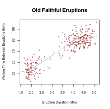
This plot is of waiting time between eruptions of Old Faithful and duration of eruptions, but it might as well be a plot of the supply line for sweater sales
Data always comes out looking like a cloud, and without using proper techniques, it is impossible to determine if this cloud gives any useful information. Econometrics is a tool to establish correlation and hopefully later, causality, using collected data points. We do this by creating an explanatory function from the data. The function is linear model and is estimated by minimizing the squared distance from the data to the line. The distance is considered an error term. This is the process of linear regression.
The Line[edit | edit source]
The point of econometrics is establishing a correlation, and hopefully, causality between two variables. The easiest way to do this is to make a line. The slope of the line will say «if we increase x by so much, then y will increase by this much» and we have an intercept that gives us the value of y when x = 0.
The equation for a line is y = a + b*x (note:a and b take on different written forms, such as alpha and beta, or beta(0) beta(1) but they always mean «intercept» and «slope»).
The problem is developing a line that fits our data. Because our data is scattered, and non-linear, it is impossible for this simple line to hit every data point. So we set our line up so that it minimizes the errors (and we need to actually minimize the squared errors). We adjust our first line, or explanatory function to have an error term, so that, given x and the error term, we can correctly come up with the right y.
y = a + b*x + error
Basic Example[edit | edit source]
After blowing our grant money on a vacation, we are pressured by the University to come up with some answers about movements of the sweater industry in Minnesota. We do not have much time, so we only collect data from two different clothing stores in Minnesota on two separate days. Fortunately for us, we get data from one day in the summer and one day in the winter. We ask both stores to tell us how many sweaters they have sold and they tell us the truth. We are looking to see how weather (temperature—independent variable) affects how many sweaters are sold (dependent variable).
We come up with the following scatter plot.
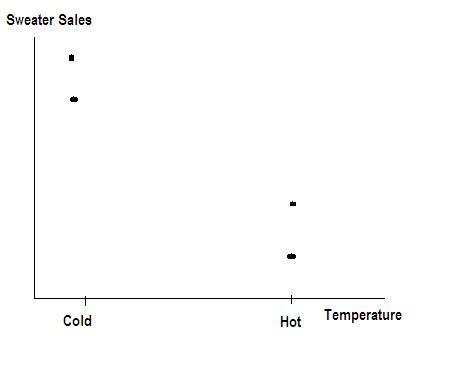
Now we can add a line (a function) to tell us the relationship of these two variables. We will minimize the sum of errors, and see what we get. The distance to the line from the cold side is +15 and the difference from the hot side to the line is -15. When we add them together, we get 15 — 15 = 0. 0 error, our line must be perfect!

Notice that our line fits the data well. The differences between the data and the function are evenly distributed ( ). So there is a relationship between temperature and sweater sales. «Hot weather increases Sweater Sales» will be the title of our famous paper! But it will be wrong, and we’ll probably be fired from our job at the University.
If we had only minimized the absolute distances between the line and the data! Well, here is a plot with an estimated line that does just that. To do this, we minimize the sum of squared errors.

Once we minimize the absolute distances between the line and the data, we have a better fit and we can declare that «cold weather increases Sweater Sales» ( )
)
Basic bivariate model[edit | edit source]
Our basic model is a line that best fits the data.

Where ![{displaystyle Y_{i}in [1,n]}](https://wikimedia.org/api/rest_v1/media/math/render/svg/4d65c458cf137609df69912d78ecb0a9295a131e) and
and ![{displaystyle X_{i}in [1,n]}](https://wikimedia.org/api/rest_v1/media/math/render/svg/e3c7780d45e3ff2dda69a53370c54a5d3e6b4fb3) , α and β are unknown parameters that must be estimated.
, α and β are unknown parameters that must be estimated. ![{displaystyle epsilon _{i}in [1,n]}](https://wikimedia.org/api/rest_v1/media/math/render/svg/6fdac3b0a1e081c8fa7f5d9ee866a9236adc6a86) is the unobserved error term. This term is an iid random variable. regression coefficient.
is the unobserved error term. This term is an iid random variable. regression coefficient.
Notes on Notation:
| Symbol | meaning |
|---|---|
| Y | Dependent Variable |
| X | Independent Variable(s) |
| α,β | Regression Coefficients |
| ε,u | Error or Disturbance term |
| ^ | Hat: Estimated |
Properties of the error term[edit | edit source]
The error term, also known as the disturbance term, is the unobserved random component which explains the difference between  and
and  . This term is the combination of four different effects.
1. Omitted Variables: in many cases, it is hard to account for every variability in the system. Cold weather increases sweater sales, but the price of heating oil may also have an effect. This was not accounted in our original model, but may be explained in our error term.
2. Nonlinearities: The actual relationship may not be linear, but all we have is a linear modeling system. At 30 degrees, 10 people buy sweaters. At 20 degrees 40 people buy sweaters. At 10 degrees 80 people buy sweaters. In our model, the error term does not take into account this nonlinearity.
3. Measurement errors: Sometimes data was not collected 100% correctly. The store told us that 10 people bought sweaters that day, but after we talked to them, 4 more people bought sweaters. The relationship still exists, but we have some error collected in the error term.
4. Unpredictable effects: No matter how well the economic model is specified, there will always be some sort of stochasticity that affects it. These effects will be accounted for by the error term.
Looking again at our OLS line in our sweater story, we a can have a look at our error terms. The error, is the distance from our data Y and our estimate Ŷ. We get an equation from this: 
next page>