Пользователя GPS-навигатора всегда интересует реальная точностьсистемы GPS-навигации и степень доверия к ее показаниям. Насколько можно приближаться к какой-либо навигационной опасности, полагаясь только на приемник GPS-навигатора? К сожалению, однозначного ответа на этот вопрос не существует. Это связано со статистическим характером ошибок GPS-навигации. Рассмотрим их подробнее.
Точность определения координат в GPS-навигации и причины ошибок GPS.
На скорость распространения радиоволн влияют ионосфера и тропосфера, ионосферная и тропосферная рефракция. Это главный, после отключения SA, источник погрешностей. Скорость радиоволн в пустоте постоянна, но при входе сигнала в атмосферу изменяется. Для сигналов от разных спутников задержка времени различна. Задержки распространения радиоволн зависят от состояния атмосферы и высоты спутника над горизонтом. Чем нижеспутник, тем больший путь проходит его сигнал через атмосферу и тем больше искажения. Большинство приемников исключают использование сигналов от спутников с возвышением над горизонтом менее 7,5 градусов.
Кроме того, атмосферные помехи зависят от времени суток. После захода солнца плотность ионосферы и ее влияние на радиосигналы уменьшается, явление, хорошо знакомое радистам-коротковолновикам. Военные и гражданские приемники GPS-навигаторов могут автономно определять атмосферную задержку сигнала, сравнивая задержки на разных частотах. Одночастотные потребительские приемники вносят приблизительную поправку на основании прогноза, передаваемого в составе навигационного сообщения. Качество этой информации в последнее время выросло, что дополнительно повысило точность GPS-навигации.

Режим SA.
Для сохранения преимущества высокой точности для военных GPS-навигаторов с марта 1990 года был введен режим ограничения доступа SA (Selective Availability), искусственно снижающий точность гражданского GPS-навигатора. При задействованном режиме SA в мирное время добавляется ошибка в несколько десятков метров. В особых случаях могут вводиться ошибки в сотни метров. Правительство США отвечает за работоспособность системы GPS перед миллионами пользователей, и можно рассчитывать, что повторное включение SA, и тем более, столь значительное снижение точности не будет введено без достаточно серьезных причин.
Загрубление точности достигается путем хаотического сдвига времени передачи псевдослучайного кода. Ошибки, возникающие от SA, — случайные и равновероятные в каждую сторону. SA влияет также на точность курса и скорости по GPS-навигатору. По этой причине неподвижный приемник часто показывает слегка изменяющиеся скорость и курс. Так что оценить степень воздействия SA можно по периодическим изменениям курса и скорости по GPS.
Погрешности в эфемеридных данных при GPS-навигации.
Прежде всего это погрешности, связанные с отклонением спутника от расчетной орбиты, неточностями часов, задержками сигнала в электронных схемах. Коррекция этих данных производится с Земли периодически, в промежутках между сеансами связи ошибки накапливаются. Ввиду малости эта группа погрешностей не имеет значения для гражданских пользователей.
Крайне редко, но могут иметь место более крупные ошибки из-за внезапных сбоев информации в устройствах памяти спутника. Если такой сбой не выявляется средствами самодиагностики, то до момента обнаружения ошибки наземной службой и передаче команды о неисправности спутник может какое-то время передавать неверную информацию. Происходит так называемое нарушение непрерывности или как часто переводят термин integrity, целостности навигации.
Влияние отраженного сигнала на точность GPS-навигации.
Кроме прямого сигнала от спутника GPS-приемник также может принять сигналы, отраженные от скал, зданий, проходящих судов так называемое характеризующие многолучевое распространение (multypath). Если прямой сигнал закрыт от приемника надстройками или такелажем судна, отраженный сигнал может быть сильнее. Этот сигнал проделывает более длинный путь, и приемник «думает», что находится дальше от спутника, чем на самом деле. Как правило, эти ошибки намного меньше 100 метров, поскольку только близко расположенные предметы способны дать достаточно сильное эхо.
Спутниковая геометрия при GPS-навигации.
Зависит от расположения приемника относительно спутников, по которым определяется позиция. Если приемник поймал четыре спутника и все они находятся на севере — спутниковая геометрия плохая. Результат ошибка до 50-100 метров или даже невозможность определения координат.

Все четыре измерения — из одного и того же направления, и область пересечения линий положений слишком велика. Но если 4 спутника будут расположены равномерно по сторонам горизонта, то точность намного возрастет. Спутниковая геометрия измеряется геометрическим фактором PDOP (Position Dilution Of Precision). Идеальному расположению спутников соответствует PDOP = 1. Большие значения говорят о плохой спутниковой геометрии.
Пригодными для навигации считаются значения PDOP меньше 6,0. В двухмерной навигации применяется HDOP (Horizontal Dilution Of Precision), меньше 4,0. Также используются вертикальный геометрический фактор VDOP, меньше 4,5, и временной TDOP, меньше 2,0. PDOP служит множителем для учета ошибок от других источников. Каждая измеренная приемником псевдодальность имеет свою погрешность, зависящую от атмосферных помех, ошибок в эфемеридах, режима SA, отраженного сигнала и так далее.
Так, если предполагаемые значения суммарных задержек сигнала по этим причинам, URE User Range Error или UERE User Equivalent Range Error, по-русски ЭДП — эквивалентная дальномерная погрешность, в сумме составляют 20 метров и HDOP = 1,5, то ожидаемая ошибка определения места будет равна 20 х 1,5 = 30 метров. Приемники GPS-навигаторов по-разному представляют информацию для оценки точности с использованием PDOP.
Кроме PDOP или HDOP, используется GQ (Geometric Quality) величина, обратная HDOP, или качественная оценка в баллах. Многие современные приемники показывают ЕРЕ (Estimated Position Error — ожидаемую ошибку позиции) непосредственно в единицах дистанции. ЕРЕ учитывает расположение спутников и прогноз погрешности сигналов для каждого спутника в зависимости от SA, состояния атмосферы, ошибок спутниковых часов, передаваемых в составе эфемеридной информации.
Спутниковая геометрия также становится проблемой при использовании приемника GPS-навигатора внутри транспортных средств, в густом лесу, горах, вблизи высоких зданий. Когда сигналы от отдельных спутников блокированы, положение оставшихся спутников определит, насколько точной будет позиция GPS, и их число покажет, может ли позиция вообще быть определена. Хороший приемник GPS-навигатора покажет не только, какие спутники используются, но и их местоположение, азимут и возвышение над горизонтом, так что вы можете определить, затруднен ли прием данного спутника.
По материалам книги Все о GPS-навигаторах.
Найман В.С., Самойлов А.Е., Ильин Н.Р., Шейнис А.И.
The error analysis for the Global Positioning System is important for understanding how GPS works, and for knowing what magnitude of error should be expected. The GPS makes corrections for receiver clock errors and other effects but there are still residual errors which are not corrected. GPS receiver position is computed based on data received from the satellites. Errors depend on geometric dilution of precision and the sources listed in the table below.
Artist’s conception of GPS Block II-F satellite in orbit
OverviewEdit
| Source | Effect (m) |
|---|---|
| Signal arrival C/A | ±3 |
| Signal arrival P(Y) | ±0.3 |
| Ionospheric effects | ±5 |
| Ephemeris errors | ±2.5 |
| Satellite clock errors | ±2 |
| Multipath distortion | ±1 |
| Tropospheric effects | ±0.5 |
| C/A | ±6.7 |
| P(Y) | ±6.0 |
Geometric Error Diagram Showing Typical Relation of Indicated Receiver Position, Intersection of Sphere Surfaces, and True Receiver Position in Terms of Pseudorange Errors, PDOP, and Numerical Errors
User equivalent range errors (UERE) are shown in the table. There is also a numerical error with an estimated value, , of about 1 meter (3 ft 3 in). The standard deviations, , for the coarse/acquisition (C/A) and precise codes are also shown in the table. These standard deviations are computed by taking the square root of the sum of the squares of the individual components (i.e., RSS for root sum squares). To get the standard deviation of receiver position estimate, these range errors must be multiplied by the appropriate dilution of precision terms and then RSS’ed with the numerical error. Electronics errors are one of several accuracy-degrading effects outlined in the table above. When taken together, autonomous civilian GPS horizontal position fixes are typically accurate to about 15 meters (50 ft). These effects also reduce the more precise P(Y) code’s accuracy. However, the advancement of technology means that in the present, civilian GPS fixes under a clear view of the sky are on average accurate to about 5 meters (16 ft) horizontally.
The term user equivalent range error (UERE) refers to the error of a component in the distance from receiver to a satellite. These UERE errors are given as ± errors thereby implying that they are unbiased or zero mean errors. These UERE errors are therefore used in computing standard deviations. The standard deviation of the error in receiver position,
, is computed by multiplying PDOP (Position Dilution Of Precision) by
, the standard deviation of the user equivalent range errors.
is computed by taking the square root of the sum of the squares of the individual component standard deviations.
PDOP is computed as a function of receiver and satellite positions. A detailed description of how to calculate PDOP is given in the section Geometric dilution of precision computation (GDOP).
for the C/A code is given by:
The standard deviation of the error in estimated receiver position , again for the C/A code is given by:
The error diagram on the left shows the inter relationship of indicated receiver position, true receiver position, and the intersection of the four sphere surfaces.
Signal arrival time measurementEdit
The position calculated by a GPS receiver requires the current time, the position of the satellite and the measured delay of the received signal. The position accuracy is primarily dependent on the satellite position and signal delay.
To measure the delay, the receiver compares the bit sequence received from the satellite with an internally generated version. By comparing the rising and trailing edges of the bit transitions, modern electronics can measure signal offset to within about one percent of a bit pulse width, , or approximately 10 nanoseconds for the C/A code. Since GPS signals propagate at the speed of light, this represents an error of about 3 meters.
This component of position accuracy can be improved by a factor of 10 using the higher-chiprate P(Y) signal. Assuming the same one percent of bit pulse width accuracy, the high-frequency P(Y) signal results in an accuracy of or about 30 centimeters.
Atmospheric effectsEdit
Inconsistencies of atmospheric conditions affect the speed of the GPS signals as they pass through the Earth’s atmosphere, especially the ionosphere. Correcting these errors is a significant challenge to improving GPS position accuracy. These effects are smallest when the satellite is directly overhead and become greater for satellites nearer the horizon since the path through the atmosphere is longer (see airmass). Once the receiver’s approximate location is known, a mathematical model can be used to estimate and compensate for these errors.
Ionospheric delay of a microwave signal depends on its frequency. It arises from ionized atmosphere (see Total electron content). This phenomenon is known as dispersion and can be calculated from measurements of delays for two or more frequency bands, allowing delays at other frequencies to be estimated.[1] Some military and expensive survey-grade civilian receivers calculate atmospheric dispersion from the different delays in the L1 and L2 frequencies, and apply a more precise correction. This can be done in civilian receivers without decrypting the P(Y) signal carried on L2, by tracking the carrier wave instead of the modulated code. To facilitate this on lower cost receivers, a new civilian code signal on L2, called L2C, was added to the Block IIR-M satellites, which was first launched in 2005. It allows a direct comparison of the L1 and L2 signals using the coded signal instead of the carrier wave.
The effects of the ionosphere generally change slowly, and can be averaged over time. Those for any particular geographical area can be easily calculated by comparing the GPS-measured position to a known surveyed location. This correction is also valid for other receivers in the same general location. Several systems send this information over radio or other links to allow L1-only receivers to make ionospheric corrections. The ionospheric data are transmitted via satellite in Satellite Based Augmentation Systems (SBAS) such as Wide Area Augmentation System (WAAS) (available in North America and Hawaii), EGNOS (Europe and Asia), Multi-functional Satellite Augmentation System (MSAS) (Japan), and GPS Aided Geo Augmented Navigation (GAGAN) (India) which transmits it on the GPS frequency using a special pseudo-random noise sequence (PRN), so only one receiver and antenna are required.
Humidity also causes a variable delay, resulting in errors similar to ionospheric delay, but occurring in the troposphere. This effect is more localized than ionospheric effects, changes more quickly and is not frequency dependent. These traits make precise measurement and compensation of humidity errors more difficult than ionospheric effects.[2]
The Atmospheric pressure can also change the signals reception delay, due to the dry gases present at the troposphere (78% N2, 21% O2, 0.9% Ar…). Its effect varies with local temperature and atmospheric pressure in quite a predictable manner using the laws of the ideal gases.[3]
Multipath effectsEdit
GPS signals can also be affected by multipath issues, where the radio signals reflect off surrounding terrain; buildings, canyon walls, hard ground, etc. These delayed signals cause measurement errors that are different for each type of GPS signal due to its dependency on the wavelength.[4]
A variety of techniques, most notably narrow correlator spacing, have been developed to mitigate multipath errors. For long delay multipath, the receiver itself can recognize the wayward signal and discard it. To address shorter delay multipath from the signal reflecting off the ground, specialized antennas (e.g., a choke ring antenna) may be used to reduce the signal power as received by the antenna. Short delay reflections are harder to filter out because they interfere with the true signal, causing effects almost indistinguishable from routine fluctuations in atmospheric delay.
Multipath effects are much less severe in moving vehicles. When the GPS antenna is moving, the false solutions using reflected signals quickly fail to converge and only the direct signals result in stable solutions.
Ephemeris and clock errorsEdit
While the ephemeris data is transmitted every 30 seconds, the information itself may be up to two hours old. Variability in solar radiation pressure[5] has an indirect effect on GPS accuracy due to its effect on ephemeris errors. If a fast time to first fix (TTFF) is needed, it is possible to upload a valid ephemeris to a receiver, and in addition to setting the time, a position fix can be obtained in under ten seconds. It is feasible to put such ephemeris data on the web so it can be loaded into mobile GPS devices.[6] See also Assisted GPS.
The satellites’ atomic clocks experience noise and clock drift errors. The navigation message contains corrections for these errors and estimates of the accuracy of the atomic clock. However, they are based on observations and may not indicate the clock’s current state.
These problems tend to be very small, but may add up to a few meters (tens of feet) of inaccuracy.[7]
For very precise positioning (e.g., in geodesy), these effects can be eliminated by differential GPS: the simultaneous use of two or more receivers at several survey points. In the 1990s when receivers were quite expensive, some methods of quasi-differential GPS were developed, using only one receiver but reoccupation of measuring points. At the TU Vienna the method was named qGPS and post processing software was developed.[citation needed]
Dilution of precision Edit
Selective availabilityEdit
GPS included a (currently disabled) feature called Selective Availability (SA) that adds intentional, time varying errors of up to 100 meters (328 ft) to the publicly available navigation signals. This was intended to deny an enemy the use of civilian GPS receivers for precision weapon guidance.
SA errors are actually pseudorandom, generated by a cryptographic algorithm from a classified seed key available only to authorized users (the U.S. military, its allies and a few other users, mostly government) with a special military GPS receiver. Mere possession of the receiver is insufficient; it still needs the tightly controlled daily key.
Before it was turned off on May 2, 2000, typical SA errors were about 50 m (164 ft) horizontally and about 100 m (328 ft) vertically.[8] Because SA affects every GPS receiver in a given area almost equally, a fixed station with an accurately known position can measure the SA error values and transmit them to the local GPS receivers so they may correct their position fixes. This is called Differential GPS or DGPS. DGPS also corrects for several other important sources of GPS errors, particularly ionospheric delay, so it continues to be widely used even though SA has been turned off. The ineffectiveness of SA in the face of widely available DGPS was a common argument for turning off SA, and this was finally done by order of President Clinton in 2000.[9]
DGPS services are widely available from both commercial and government sources. The latter include WAAS and the U.S. Coast Guard’s network of LF marine navigation beacons. The accuracy of the corrections depends on the distance between the user and the DGPS receiver. As the distance increases, the errors at the two sites will not correlate as well, resulting in less precise differential corrections.
During the 1990–91 Gulf War, the shortage of military GPS units caused many troops and their families to buy readily available civilian units. Selective Availability significantly impeded the U.S. military’s own battlefield use of these GPS, so the military made the decision to turn it off for the duration of the war.
In the 1990s, the FAA started pressuring the military to turn off SA permanently. This would save the FAA millions of dollars every year in maintenance of their own radio navigation systems. The amount of error added was «set to zero»[10] at midnight on May 1, 2000 following an announcement by U.S. President Bill Clinton, allowing users access to the error-free L1 signal. Per the directive, the induced error of SA was changed to add no error to the public signals (C/A code). Clinton’s executive order required SA to be set to zero by 2006; it happened in 2000 once the U.S. military developed a new system that provides the ability to deny GPS (and other navigation services) to hostile forces in a specific area of crisis without affecting the rest of the world or its own military systems.[10]
On 19 September 2007, the United States Department of Defense announced that future GPS III satellites will not be capable of implementing SA,[11] eventually making the policy permanent.[12]
Anti-spoofingEdit
Another restriction on GPS, antispoofing, remains on. This encrypts the P-code so that it cannot be mimicked by a transmitter sending false information. Few civilian receivers have ever used the P-code, and the accuracy attainable with the public C/A code was much better than originally expected (especially with DGPS), so much so that the antispoof policy has relatively little effect on most civilian users. Turning off antispoof would primarily benefit surveyors and some scientists who need extremely precise positions for experiments such as tracking tectonic plate motion.
RelativityEdit
Theory of Relativity introduces several effects that need to be taken into account when dealing with precise time measurements. First, according to special relativity time passes differently for objects in relative motion. That is known as «kinetic» time dilation: in an inertial reference frame, the faster an object moves, the slower its time appears to pass
(as measured by the frame’s clocks). General relativity takes into account also the effects that gravity has on the passage of time. In the context of GPS the most prominent correction introduced by general relativity is gravitational time dilation: the clocks located deeper in the gravitational potential well (i.e. closer to the attracting body) appear to tick slower.
Satellite clocks are slowed by their orbital speed but sped up by their distance out of the Earth’s gravitational well.
Special Relativity (SR)Edit
SR predicts that as the velocity of an object increases (in a given frame), it’s time slows down (as measured in that frame). For instance, the frequency of the atomic clocks moving at GPS orbital speeds will tick more slowly than stationary clocks by a factor of where the orbital velocity is v = 4 km/s and c = the speed of light. The result is an error of about -7.2 μs/day in the satellite. The SR effect is due to the constant movement of GPS clocks relative to the Earth-centered, non-rotating approximately inertial reference frame. In short, the clocks on the satellites are slowed down by the velocity of the satellite. This time dilation effect has been measured and verified using the GPS.
General Relativity (GR)Edit
SR allows to compare clocks only in a flat spacetime, which neglects gravitational effects on the passage of time. According to GR, the presence of gravitating bodies (like Earth) curves spacetime, which makes comparing clocks not as straightforward as in SR. However, one can often account for most of the discrepancy by the introduction of gravitational time dilation, the slowing down of time near gravitating bodies. In case of the GPS, the receivers are closer to Earth than the satellites, causing the locks at the altitude of the satellite to be faster by a factor of 5×10⁻¹⁰, or about +45.8 μs/day. This gravitational frequency shift is measurable. During early development some believed that GPS would not be affected by GR effects, but the Hafele–Keating experiment showed it would be.
Combined kinetic and gravitational time dilationsEdit
Combined, these sources of time dilation cause the clocks on the satellites count extra +38 microseconds per day, compared to the clocks on the ground. This is a difference of 4.465 parts in 1010.[13] Without correction, errors of roughly 11.4 km/day would accumulate in the position.[14] This initial pseudorange error is corrected in the process of solving the navigation equations. In addition, the elliptical, rather than perfectly circular, satellite orbits cause the time dilation and gravitational frequency shift effects to vary with time. This eccentricity effect causes the clock rate difference between a GPS satellite and a receiver to increase or decrease depending on the altitude of the satellite.
| Time dilation | Value | Notes |
|---|---|---|
| Kinetic | -7.2 μs/day | Clocks slowed in satellites due to Velocity |
| Gravitational | +45.8 μs/day | Clocks sped up in satellites due to higher altitude |
| Total (Combined) | +38.6 μs/day |
To compensate for the discrepancy, the frequency standard on board each satellite is given a rate offset prior to launch, making it run slightly slower than the desired frequency on Earth; specifically, at 10.22999999543 MHz instead of 10.23 MHz.[15] Since the atomic clocks on board the GPS satellites are precisely tuned, it makes the system a practical engineering application of the scientific theory of relativity in a real-world environment.[16] Placing atomic clocks on artificial satellites to test Einstein’s general theory was proposed by Friedwardt Winterberg in 1955.[17]
CalculationsEdit
To calculate the amount of daily time dilation experienced by GPS satellites relative to Earth we need to separately determine the amounts due to satellite’s velocity and altitude, and add them together.
Kinetic time dilationEdit
The amount due to velocity will be determined using the Lorentz transformation. The time measured by an object moving with velocity changes by (the inverse of) the Lorentz factor:
For small values of v/c this approximates to:
The GPS satellites move at 3874 m/s relative to Earth’s center.[15] We thus determine:
This difference of 8.349×10⁻¹¹ represents the fraction by which the satellites’ clocks tick slower than the stationary clocks. It is then multiplied by the number of nanoseconds in a day:
That is the satellites’ clocks lose 7214 nanoseconds a day due to their velocity.
- Note that this speed of 3874 m/s is measured relative to Earth’s center rather than its surface where the GPS receivers (and users) are. This is because Earth’s equipotential makes net time dilation equal across its geodesic surface.[18] That is, the combination of Special and General effects make the net time dilation at the equator equal to that of the poles, which in turn are at rest relative to the center. Hence we use the center as a reference point to represent the entire surface.
Gravitational time dilationEdit
The amount of dilation due to gravity will be determined using the gravitational time dilation equation:
where is the time passed at a distance from the center of the Earth and is the time passed for a far away observer.
For small values of this approximates to:
Determine the difference between the satellite’s time and Earth time :
Earth has a radius of 6,357 km (at the poles) making = 6,357,000 m and the satellites have an altitude of 20,184 km[15] making their orbit radius = 26,541,000 m. Substituting these in the above equation, with Earth mass M = 5.974×1024, G = 6.674×10⁻¹¹, and c = 2.998×10⁸ (all in SI units), gives:
This represents the fraction by which the clocks at satellites’ altitude tick faster than on the surface of the Earth. It is then multiplied by the number of nanoseconds in a day:
That is the satellites’ clocks gain 45850 nanoseconds a day due to gravitational time dilation.
Combined time dilation effectsEdit
These effects are added together to give (rounded to 10 ns):
- 45850 – 7210 = 38640 ns
Hence the satellites’ clocks gain approximately 38,640 nanoseconds a day or 38.6 μs per day due to relativity effects in total.
In order to compensate for this gain, a GPS clock’s frequency needs to be slowed by the fraction:
- 5.307×10⁻¹⁰ – 8.349×10−11 = 4.472×10⁻¹⁰
This fraction is subtracted from 1 and multiplied by the pre-adjusted clock frequency of 10.23 MHz:
- (1 – 4.472×10−10) × 10.23 = 10.22999999543
That is we need to slow the clocks down from 10.23 MHz to 10.22999999543 MHz in order to negate both time dilation effects.
Sagnac distortionEdit
GPS observation processing must also compensate for the Sagnac effect. The GPS time scale is defined in an inertial system but observations are processed in an Earth-centered, Earth-fixed (co-rotating) system. A coordinate transformation is thus applied to convert from the inertial system to the ECEF system. The resulting signal run time correction has opposite algebraic signs for satellites in the Eastern and Western celestial hemispheres. Ignoring this effect will produce an east–west error on the order of hundreds of nanoseconds, or tens of meters in position.[19]
Natural sources of interferenceEdit
Since GPS signals at terrestrial receivers tend to be relatively weak, natural radio signals or scattering of the GPS signals can desensitize the receiver, making acquiring and tracking the satellite signals difficult or impossible.
Space weather degrades GPS operation in two ways, direct interference by solar radio burst noise in the same frequency band[20] or by scattering of the GPS radio signal in ionospheric irregularities referred to as scintillation.[21] Both forms of degradation follow the 11 year solar cycle and are a maximum at sunspot maximum although they can occur at any time. Solar radio bursts are associated with solar flares and coronal mass ejections (CMEs)[22] and their impact can affect reception over the half of the Earth facing the sun. Scintillation occurs most frequently at tropical latitudes where it is a night time phenomenon. It occurs less frequently at high latitudes or mid-latitudes where magnetic storms can lead to scintillation.[23] In addition to producing scintillation, magnetic storms can produce strong ionospheric gradients that degrade the accuracy of SBAS systems.[24]
Artificial sources of interferenceEdit
In automotive GPS receivers, metallic features in windshields,[25] such as defrosters, or car window tinting films[26] can act as a Faraday cage, degrading reception just inside the car.
Man-made EMI (electromagnetic interference) can also disrupt or jam GPS signals. In one well-documented case it was impossible to receive GPS signals in the entire harbor of Moss Landing, California due to unintentional jamming caused by malfunctioning TV antenna preamplifiers.[27][28] Intentional jamming is also possible. Generally, stronger signals can interfere with GPS receivers when they are within radio range or line of sight. In 2002 a detailed description of how to build a short-range GPS L1 C/A jammer was published in the online magazine Phrack.[29]
The U.S. government reported that such jammers were used occasionally during the War in Afghanistan, and the U.S. military destroyed six GPS jammers during the Iraq War, including one that was destroyed with a GPS-guided bomb, noting the ineffectiveness of the jammers used in that situation.[30] A GPS jammer is relatively easy to detect and locate, making it an attractive target for anti-radiation missiles. The UK Ministry of Defence tested a jamming system in the UK’s West Country on 7 and 8 June 2007.[citation needed]
Some countries allow the use of GPS repeaters to allow the reception of GPS signals indoors and in obscured locations; while in other countries these are prohibited as the retransmitted signals can cause multi-path interference to other GPS receivers that receive data from both GPS satellites and the repeater. In the UK Ofcom now permits the use of GPS/GNSS Repeaters[31] under a ‘light licensing’ regime.
Due to the potential for both natural and man-made noise, numerous techniques continue to be developed to deal with the interference. The first is to not rely on GPS as a sole source. According to John Ruley, «IFR pilots should have a fallback plan in case of a GPS malfunction».[32] Receiver Autonomous Integrity Monitoring (RAIM) is a feature included in some receivers, designed to provide a warning to the user if jamming or another problem is detected. The U.S. military has also deployed since 2004 their Selective Availability / Anti-Spoofing Module (SAASM) in the Defense Advanced GPS Receiver (DAGR).[33] In demonstration videos the DAGR was shown to detect jamming and maintain its lock on the encrypted GPS signals during interference which caused civilian receivers to lose lock.
See alsoEdit
- GPS augmentation
NotesEdit
- ^ The same principle, and the math behind it, can be found in descriptions of pulsar timing by astronomers.
- ^ Navipedia: Troposphere Monitoring
- ^ Navipedia: Tropospheric Delay
- ^ Navipedia: Multipath
- ^ «IPN Progress Report 42-159 (2004)» (PDF).
- ^ SNT080408. «Ephemeris Server Example». Tdc.co.uk. Archived from the original on January 12, 2009. Retrieved 2009-10-13.
- ^ «Unit 1 – Introduction to GPS». Archived from the original on April 29, 2009.
- ^ Grewal (2001), p. 103.
- ^ «President Clinton Orders the Cessation of GPS Selective Availability».
- ^ a b «Statement by the President regarding the United States’ Decision to Stop Degrading Global Positioning System Accuracy». Federal Aviation Administration. May 1, 2000. Archived from the original on 2011-10-21. Retrieved 2013-01-04.
- ^ «DoD Permanently Discontinues Procurement Of Global Positioning System Selective Availability». DefenseLink. September 18, 2007. Archived from the original on February 18, 2008. Retrieved 2008-02-20.
- ^ «Selective Availability». National space-based Positioning, Navigation, and Timing Executive Committee. Archived from the original on January 13, 2008. Retrieved 2008-02-20.
- ^ Rizos, Chris. University of New South Wales. GPS Satellite Signals Archived 2010-06-12 at the Wayback Machine. 1999.
- ^ Faraoni, Valerio (2013). Special Relativity (illustrated ed.). Springer Science & Business Media. p. 54. ISBN 978-3-319-01107-3. Extract of page 54
- ^ a b c The Global Positioning System by Robert A. Nelson Via Satellite Archived 2010-07-18 at the Wayback Machine, November 1999
- ^ Pogge, Richard W.; «Real-World Relativity: The GPS Navigation System». Retrieved 25 January 2008.
- ^ «Astronautica Acta II, 25 (1956)». 1956-08-10. Retrieved 2009-10-23.
- ^ S. P. Drake (January 2006). «The equivalence principle as a stepping stone from special to general relativity» (PDF). Am. J. Phys., Vol. 74, No. 1. pp. 22–25.
- ^ Ashby, Neil Relativity and GPS. Physics Today, May 2002.
- ^ Cerruti, A., P. M. Kintner, D. E. Gary, A. J. Mannucci, R. F. Meyer, P. H. Doherty, and A. J. Coster (2008), Effect of intense December 2006 solar radio bursts on GPS receivers, Space Weather, doi:10.1029/2007SW000375, October 19, 2008
- ^ Aarons, Jules; Basu, Santimay (1994). «Ionospheric amplitude and phase fluctuations at the GPS frequencies». Proceedings of ION GPS. 2: 1569–1578.
- ^ S. Mancuso and J. C. Raymond, «Coronal transients and metric type II radio bursts. I. Effects of geometry, 2004, Astronomy and Astrophysics, v.413, p.363-371′
- ^ Ledvina, B. M.; J. J. Makela & P. M. Kintner (2002). «First observations of intense GPS L1 amplitude scintillations at midlatitude». Geophysical Research Letters. 29 (14): 1659. Bibcode:2002GeoRL..29.1659L. doi:10.1029/2002GL014770. S2CID 133701419.
- ^ Tom Diehl, Solar Flares Hit the Earth- WAAS Bends but Does Not Break, SatNav News, volume 23, June 2004.
- ^ «I-PASS Mounting for Vehicles with Special Windshield Features» (PDF). Archived from the original (PDF) on March 26, 2010.
- ^ «3M Automotive Films».. Note that the ‘Color Stable’ films are specifically described as not interfering with satellite signals.
- ^ «The Hunt for RFI». GPS World. 1 January 2003.
- ^ «EMC compliance club «banana skins» column 222″. Compliance-club.com. Retrieved 2009-10-13.
- ^ Low Cost and Portable GPS Jammer. Phrack issue 0x3c (60), article 13. Published December 28, 2002.
- ^ American Forces Press Service. Centcom charts progress. March 25, 2003. Archived December 3, 2009, at the Wayback Machine
- ^ [1] Ofcom Statement on Authorisation regime for GNSS repeaters
- ^ Ruley, John. AVweb. GPS jamming. February 12, 2003.
- ^ US Army DAGR page Archived 2012-08-05 at archive.today
ReferencesEdit
- Grewal, Mohinder S.; Weill, Lawrence Randolph; Andrews, Angus P. (2001). Global positioning systems, inertial navigation, and integration. John Wiley and Sons. ISBN 978-0-471-35032-3.
- Parkinson; Spilker (1996). The global positioning system. American Institute of Aeronautics & Astronomy. ISBN 978-1-56347-106-3.
- Webb, Stephen (2004). Out of this world: colliding universes, branes, strings, and other wild ideas of modern physics. Springer. ISBN 0-387-02930-3. Retrieved 2013-08-16.
External linksEdit
- GPS.gov—General public education website created by the U.S. Government
- GPS SPS Performance Standard—The official Standard Positioning Service specification (2008 version).
- GPS SPS Performance Standard—The official Standard Positioning Service specification (2001 version).
Estimated Position Error…..

23rd Jun 2007, 14:20
Thread Starter
Join Date: Jul 2006
Location: ‘tween posts
Posts: 196
Likes: 0
Received 0 Likes
on
0 Posts
Estimated Position Error…..
Hello every one ,
Reading my books on navigation and trying to figure out how did they (whoever they are) arrive at a figure of 0.28nm as a threshold for estimate position error ???
can anyone help?
thanks,

Last edited by gearpins; 23rd Jun 2007 at 14:31.

25th Jun 2007, 06:41
Thread Starter
Join Date: Jul 2006
Location: ‘tween posts
Posts: 196
Likes: 0
Received 0 Likes
on
0 Posts
standing by
anyone please?
25th Jun 2007, 07:02
Moderator
Join Date: Feb 2000
Location: UK
Posts: 14,037
You aren’t giving us much to work on!
In what circumstances does the author of the book give the value? Position measured how? — DR?/RNAV?/INS?, how long into flight?, etc.
G
25th Jun 2007, 13:19
Thread Starter
Join Date: Jul 2006
Location: ‘tween posts
Posts: 196
Likes: 0
Received 0 Likes
on
0 Posts
sorry about that
OK here is an extract from FCOM A320
EPE (RATE or THRESHOLD)
REMARK
IRS/GPS
(FOM� + 100�) in meters
FOM = Figure of Merit of GPS
If above 0.28 NM the GPS position is rejected.
IRS/DME/DME
Tends towards 0.28 NM
EPE decreases from initial value to 0.28 Nm.
IRS/VOR/DME
0.1 NM + 0.05 X DME DIST minimum : 0.28 NM
EPE increases or decreases as the distance between the a/c and the VOR/DME.
IRS ONLY
+ 8 NM/h for the first 21 min.
+ 2 NM/h after
EPE increases continuously
sorry once again for the lack of clarity before
25th Jun 2007, 14:58
Moderator
Join Date: Feb 2000
Location: UK
Posts: 14,037
Is that not saying that if the error is greater than 0.28nm it rejects it, it doesn’t look like a statement of error calculation to me.
G
25th Jun 2007, 15:49
Join Date: Sep 1998
Location: wherever
Age: 53
Posts: 1,616
Likes: 0
Received 0 Likes
on
0 Posts
Looks like Airbus don’t want an epe less than .28 uless GPS is valid and used.
May well have something to do with the implamentation of RNP when the system was designed. As RNP approaches at one time also specified the nav mode eg. RNAV(GNSS)
B-RNAV = RNP 5
P-RNAV = RNP 1
Default Approach value on our brazilian/honeywell equipment is RNP.3
As RNP is stll evolving I woudn’t spend too much time worrying as by the time you’ve figured it out the game may have changed.
26th Jun 2007, 23:00
Thread Starter
Join Date: Jul 2006
Location: ‘tween posts
Posts: 196
Likes: 0
Received 0 Likes
on
0 Posts
just wondering..
All I am trying to do is figure why is the value 0.28?? and not say 2 or some other convenient number. I am sure its for a good reason. just trying to get to the history behind it…
Any Navigation guru out there..??
28th Jun 2007, 11:04
Join Date: Apr 2003
Location: Not commuting home
Age: 45
Posts: 4,120
I think you misinterpret the information given. On the very next FCOM page, there is some explanatory text and regulatory requirements to which the aircraft had been certified.
ENR 2 NM, Terminal 1 NM and APCH 0,5 NM (0,3 with GPS).
Aircraft itself estimates the probable positon error (based on available data sources and time from initialization / last update). This EPE value is evaluated against the certification requirements and pilot is warned whenever accuracy limit is not satisfied.
What you quote is a very in-depth knowledge on how exactly is the EPE calculated.
For instance the IRS mode with DME/DME updating the EPE may be as low as 0,28 NM. Essentially the manufacturer states that 0,28 NM is the best achievable precision in IRS/DME/DME mode. Why not 2 NM? Beacuse their equipment is much better than that. Why not 0,1 NM? I bet they wish but IRS/DME/DME installation just cannot do it.

2nd Jul 2007, 03:10
Thread Starter
Join Date: Jul 2006
Location: ‘tween posts
Posts: 196
Likes: 0
Received 0 Likes
on
0 Posts
flt detent, thanks, that cleared it up a bit for me.
I was wondering if .28 nm was also a regulatory requirement?

Posting Rules
You may not post new threads
You may not post replies
You may not post attachments
You may not edit your posts
HTML code is Off
The Estimated Position Error (abbreviated «EPE») is shown right next
to the Current Position Lock buttons. This value represents the ex-
pected error from a benchmark location. In other words, if the EPE
shows 50 feet, then the position shown by the unit is estimated to be
within 50 feet of the actual location.
This also gives you an indicator of the fix quality the unit currently has.
The smaller the position error number, the better (and more accurate)
the fix is. If the position error flashes dashes, then the unit hasn’t
locked onto the satellites, and the number shown isn’t valid.
Satellite Display
A white circle that serves as a graphical view of the satellites overhead
fills much of the right half of the screen. Each satellite is shown on the
circular chart relative to your position. The GPS receiver is tracking sat-
ellites that are in blue type. The receiver hasn’t locked onto a satellite if
the number is in dark blue, so it isn’t being used to track the position.
Lat/Lon Coordinates
Beneath the Satellite Display, you can see your Coordinates in Latitude
and Longitude. These numbers can be used to pinpoint your location on
any map, or to create contacts at your position on another GPS.
Transfer Data
In addition to storing media files such as music and pictures, you can
use your MMC or SD Card to store and transfer GPS data recorded on
the unit. This is a handy way to save contacts that you’ve created,
Trails of places you’ve been, and routes you’ve set up.
To save data to your memory card, or to load data from your memory
card, choose the
command from the Options Menu. Tell
T
D
RANSFER
ATA
the iWAY whether you want to
data for the iWAY to display and
L
OAD
use or
data to the card to store or transfer it to another GPS unit.
S
AVE
If you want to Load data, choose the dropdown box and make sure to
select the filename of the GPS Data File you want to load. If you are
Saving data, you can select the Filename text box to enter a new name
describing the data you’re saving.
GPS Simulator
The iWAY offers a GPS Simulator option allowing it to simulate the
navigation of a route. When you turn on the Simulator, the iWAY pre-
tends it has a GPS lock at the current location, then begins moving
along the current route as though you are following it.
45
Inertial position estimator (INAV)
Position estimator is a vital component for navigation subsystem. It takes data from all available sensors and fuses them together to figure out coordinates and velocities in the local frame of reference. All navigational decisions are made based on estimated position/velocity data.
It is currently desined for multirotors.
Principle of operation
The key sensor for INAV is an accelerometer. Measured acceleration is translated from body-fixed frame to local NEU coordinates and integrated to yield velocities in North, East and Up directions. Velocity is further integrated to produce coordinates.
As accelerometer tend to drift, estimated velocities and coordinates tend to drift as well. This accumulated error is corrected from various reference sources — GPS, BARO, SONAR. Position estimator also maintains estimated position error for horizontal (X-Y) and vertical (Z) position.
When reference source is not available for some reason, estimated position error increases until it reaches a certain threshold. Beyond that threshold position is no longer updated and marked invalid until a valid reference source is available avain. This allows, for example, to fly through short (measured in seconds) GPS outages.
Using multiple sensors for estimation allows to filter noisy data (e.g. from barometer), interpolate between rare readings (e.g. from GPS), and immediately react on fast motion changes (using accelerometers) in the same time.
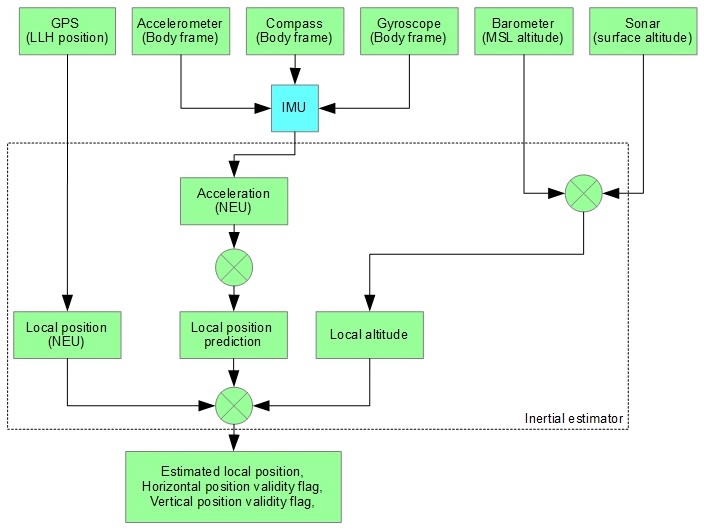
Data soures
The following reference sources (with corresponding parameters for weight) are available for altitude and climb rate:
- Barometer — altitude (inav_w_z_baro_p)
- Barometer — velocity (inav_w_z_baro_v)
- Sonar — altitude (inav_w_z_sonar_p)
- Sonar — velocity (inav_w_z_sonar_v)
- GPS — altitude (inav_w_z_gps_p)
- GPS — velocity (inav_w_z_gps_v)
Sonar is optional source, it’s only used when available and valid data received. GPS altitude is very noisy and is limited to FIXED_WING aircraft (experimental and untested).
The following reference sources (with corresponding parameters for weight) are available for position and velocity:
- GPS — position (inav_w_xy_gps_p)
- GPS — velocity (inav_w_xy_gps_v)
Dead reckoning and handling sensor unavailability
-
Enable dead reckoning (inav_enable_dead_reckoning)
-
Dead reckoning — position (inav_w_xy_dr_p)
-
Dead reckoning — velocity (inav_w_xy_dr_v)
-
Velocity decay rate, XY-axis (inav_w_xy_res_v)
-
Velocity decay rate, Z-axis (inav_w_z_res_v)
Estimated position error thresholds
- Maximum acceptable position error (inav_max_eph_epv)
- Position error for SONAR sensor (inav_sonar_epv)
- Position error for BARO sensor (inav_baro_epv)
GPS delay compensation
GPS data is not updated instantly. GPS module needs time to calculate new position and velocity. INAV has means of compensating for this delay. Expected GPS delay in milliseconds is controlled by inav_gps_delay_ms parameter. Typical value for GPS delay is 200ms.
Position and altitude PID controllers
PID regulators in ALTHOLD mode (Z-controller)
ALTHOLD mode uses two PIDs — ALT and VEL. Navigation Z-controller functional diagram is shown below:

ALT PID
Actually ALT PID parameters control two P-controllers: Position-to-Velocity and Velocity-to-Acceleration
- ALT_P — defines how fast quad will attempt to compensate for altitude error, converts altitude error to desired vertical velocity (climb rate)
- ALT_I — not used
- ALT_D — not used
VEL PID
This PID-controller is an Acceleration-to-Throttle controller
- VEL_P — defined how much throttle quad will add/reduce to achieve desired velocity
- VEL_I — controls compensation for hover throttle (and vertical air movement, thermals). This can be zero if hover throttle is precisely 1500us. Too much VEL I will lead to vertical oscillations, too low VEL I will cause drops or jumps when ALTHOLD is enabled, very low VEL I can result in total inability to maintain altitude
- VEL_D — acts as a dampener for acceleration. VEL D will resist any velocity change regardless of its nature (requested by VEL P and VEL I or induced by wind).
PID regulators in POSHOLD/RTH/WP modes (XY-controller)
XY-controller uses two PIDs — POS and POSR

POS PID
This is a Position-to-Velocity P-controller active in POSHOLD, RTH and WP modes
- POS_P — translates position error to desired velocity to reach the target
- POS_I — not used
- POS_D — not used
POSR PID
Position rate PID-controller, controls Velocity-to-Acceleration
- POSR_P — controls acceleration to achieve desired velocity
- POSR_I — controls compensation for side wind or other disturbances. In totally calm air POSR I can be close to zero
- POSR_D — dampens response from P and I components; Tests indicate that this one can be zero at all times
Output of POSR PID-controller is desired acceleration which is directly translated to desired lean angles.
Coordinate systems
Navigation operates in 3 different coordinate systems.
LLH (Geographic) Coordinate System
Represents position on or above earth with a latitude, longitude and height value. Height is defined as altitude above the mean sea level.

NEU Coordinate System
- The x axis is aligned with the vector to the north pole (tangent to meridians).
- The y axis points to the east side (tangent to parallels)
- The z axis points up from the center of the earth
This is a classical cartesian coordinate system where the 3 axes are orthogonal to each other.
The units for the NEU coordinate system are centimetres.
Frames of reference
Global (geodetic) frame of reference
This frame of reference defines coordinates in LLH coordinate system. This frame of reference is not used directly by the code and is provided as an interface for defining waypoints and receiving reference data from GPS.
Local frame of reference
This frame of reference defines coordinate in NEU coordinate system relative to a GPS Origin point. GPS origin is defined as a point where GPS fix with sufficient accuracy was firstly acquired. GPS Origin is usually a point of launch. Most calculations are done in this frame of reference.
Body-fixed frame of reference
Attached to the aircraft.
- The x axis points in forward direction (as defined by geometry and not by movement) (roll axis)
- The y axis points to the right (geometrically) (pitch axis)
- The z axis points upwards (geometrically) (yaw axis)
This frame of reference is used to read sensor data and calculate lean angles. Usually the only operations in this frame of reference are coordinate transformations to/from local frame of reference.
1. Introduction
Many types of navigation services, such as applications on smartphones and automotive navigation systems, are becoming popular. These services play an important role in intelligent transportation systems (ITSs). However, they require highly accurate positioning, especially in urban areas. One technology that is important for providing location information such as latitude and longitude is the Global Navigation Satellite System (GNSS). Position information determined by GNSS usually is inaccurate by a few meters or more, and research has been performed to reduce the error. One promising technology for acquiring accurate location data is real-time kinematic (RTK) positioning (Sakai, 2003). In the best-case scenario, RTK positioning can provide location information with an error of only a few centimeters. Owing to its low cost and small size, the RTK positioning device is expected to be used widely. However, its positioning accuracy is not good where signal reception from satellites is unstable, especially in urban canyons. RTK accuracy depends on the environment, such as when buildings shadow signals from a GNSS satellite, so it is difficult to realize accurate navigation with RTK positioning in a city’s downtown area. One solution for solving the challenges in an urban environment is to select a satellite to eliminate signal shading by buildings. An elevation angle mask (Misra and Enge, 2001) is a technique that provides accurate position information in cities by employing satellites that exist at higher-elevation angle spaces. However, such methods for selecting satellites sometimes reduce the number of usable satellites, so accuracy does not increase as expected. Therefore, the accuracy of GNSS positioning in urban areas is challenging in general.
However, we believe that there is an alternative approach wherein applying a cognitive methodology provides user satisfaction for services such as car navigation. The main stream of the research on GNSS is increasing accuracy. However, we sometimes have a problem of car navigation because of low accuracy of position. If the positioning accuracy is not good because of the conditions, we expect that a navigation application provides an optimal solution. For example, if the accuracy of position is not good, a navigation system can lead a user to a location where the accuracy is better. We would like to call such navigation system as a cognitive navigation system. Therefore, we would like to apply the Cognitive Infocommunications (CogInfoCom) approach (Baranyi and Csapo, 2012; Baranyi et al., 2015). This idea extends human cognitive capabilities and would even enable life support.
Figure 1 shows the CogInfoCom concept for a location-based service (LBS). The original CogInfoCom architecture is shown in Figure 1 (left). A communication device offers an opportunity for users to interact with the environment by using a network and an autonomous cognitive system with sensors and Internet of Things devices. Figure 1 (right) depicts one implementation of the CogInfoCom system to an LBS, namely, an automotive navigation system. Clearly, LBSs are one of the most important services and are strongly affected by situations. In this implementation, we introduce an error map (Figure 2) that offers a level of error for GNSS positioning to improve navigation if the GNSS signal is weak or noisy. CogInfoCom makes an environment intelligent and provides information automatically.
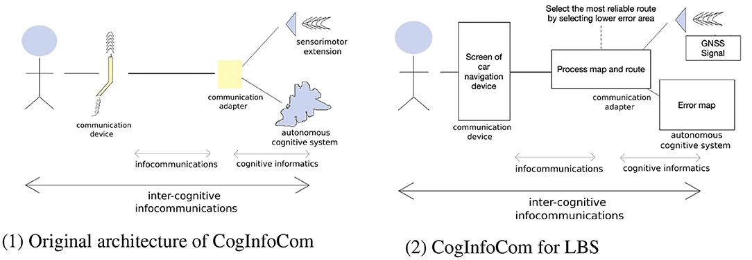
Figure 1. Error mapping for the CogInfoCom architecture.
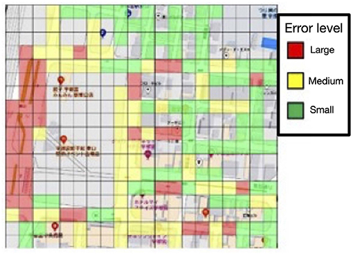
Figure 2. An example of an error map.
In the next section, we propose a new technique that increases the accuracy of GNSS positioning and the usability of LBSs by providing the error level of a specific location. We mention the difficulty of GNSS positioning and related works such as techniques for multipath shadowing environments or multi-GNSS receivers. Section 3 discusses the objectives of this research, and section 4 presents the pre-examination results to explain the characteristics of the GNSS positioning error. In section 5, details of the proposed method are discussed. The proposed methods are evaluated in section 6, and examples of how to apply the error map are proposed in section 7. Finally, section 8 concludes and discusses further studies.
2. Problems and Related works
2.1. Characteristics of the GNSS Error
As described in the previous section, one of the issues related to reducing the accuracy of GNSS is errors. A GNSS positioning error can occur for several reasons. Such an error can be caused by any of the following: the satellite’s clock, the orbit of a satellite, noise from the convection of air in the ionosphere, noise of a GNSS receiver, or multipaths (Sakai, 2003). An error that is caused by a clock’s satellite or the satellite’s orbit relates to the satellite itself, so it is possible to reduce the error if more than two receivers obtain a signal from the same satellite. In widely used techniques such as the Saastamoinen model (Saastamoinen, 1973a,b,c) and the Klobuchar model (Klobuchar, 1987), an error caused by noise from the GNSS receiver depends on the baseline (Satirapod and Chalermwattanachai, 2005). Therefore, it is possible to remove the miscalculation as a common error if there are two neighbor receivers. The remaining error depends on shadows, which cause reflections and increase the signal paths from GNSS satellites, and such reflections interfere with the original signal. Such an error varies, depending on the environment, and is difficult to predict. Also, the objects’ shadows reduce the number of GNSS satellites from a particular receiver that secures the signal and increases error. The shadowing environment causes errors that are difficult to remove, and the levels of error depend on the environment. Therefore, it is important to handle these types of errors for an LBS.
2.2. Coordinated Positioning
One approach for reducing errors is coordinated positioning, which minimizes miscalculations that are caused by sharing information among several receivers. The idea is similar to RTK positioning and removing the common receiver errors. The coordinated positioning can detect multipaths and eliminate the satellite that causes them (Osechas et al., 2015) to increase accuracy. A Differential Global Positioning System (DGPS) is one type of coordinated positioning. The reference station distributes correction information to neighboring receivers. Accordingly, a simplified DGPS is proposed (Miyata et al., 1996; Miyata and Sakitani, 1997). This system offers accurate positioning data by processing the cross-correlation of positioning data of two receivers. There is also a method for grouping the characteristics of GNSS receivers, such as an error-reduction method for the receivers that move together (Odaka et al., 2011) and to reduce multipaths by using numerous antennas on an automobile (Kubo et al., 2017).
2.3. Error Correction by a Map
A map is an important parameter for increasing the positioning accuracy and provides both correction and height information (Iwase et al., 2013). The information provided by a map is increasing, such as 3D maps. We also propose a method to provide DGPS correction data by combining map information and the location of an automobile (Rohani et al., 2016).
3. Estimating the Error of GNSS
In this section, we present the results of an experiment that considers a method to determine an estimated position error. As explained in the previous section, it is difficult to eliminate errors caused by a multipath. Table 1 presents the methods used in previous studies. These methods used the pseudorange. However, for a low-cost GNSS device such as a smartphone, the positioning function is a black box, and it is difficult to see the pseudorange information. Therefore, it is necessary to use only position data, with no internal data from the GNSS receiver. A way to use the group characteristics of GNSS receivers is to apply only the position data. However, because it is assumed to be stationary, it requires developing an error-reduction method that uses only the mobile receiver’s position data. We have been developing some methods to reduce errors that relate to multipath under the restrictions mentioned. In the remainder of this section, we will discuss our methods.
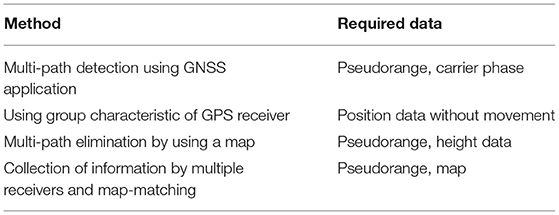
Table 1. Related works.
3.1. Method 1: Using the Common Temporal Error
We studied a method that focuses on how a common temporal error occurs in nearby receivers for the GNSS (Nakamura, 2018). The delay due to the convection of air in the ionosphere causes the main GNSS positioning error. If the distance between two receivers is small, both have the same effect caused by the delay due to the convection of air in the ionosphere and may have a common error. However, if each receiver obtains a signal from a different GNSS satellite, the pseudorange should vary and have different error patterns. Therefore, it is necessary to use the same GNSS satellite. To prove the effectiveness of this idea, we designed a system model (Figure 3) and performed a trial. As a result, accuracy improved by 0.5–1.6 m.
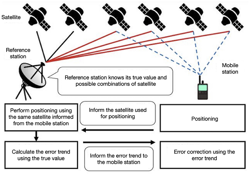
Figure 3. System model of using a common temporal error.
3.2. Method 2: Using a Bias of the Positioning Error by Multipath
This idea uses an error bias caused by multipath between neighboring receivers. In our previous research (Kitani et al., 2012), the error of neighboring receivers is biased. In this method, two receivers were placed on top of the roof of a car with the same distance, and the error of position was observed. This automobile was moving straight, and the environment alternates between not being in shadow and being in shadow. If the observed error of the two receivers fluctuates widely, both are affected for the same reason. In this case, we can understand that both receivers are affected by multipath, and we can add a corrected point by using a previously accurate result in the shadowed environment.
3.3. Method 3: Error Map
Methods 1 and 2 were designed to reduce errors. However, our idea is different in that if we know the location is shadowed and what the possible error level is, we can adapt the situation. We would like to propose a new idea, an error map, for that purpose. Figure 2 shows an example of an error map in which different colors display the multipath’s level of error. For example, if we know that the location has a poor error level, we can either change a shadow mask to eliminate the low-accuracy satellite or select a route with a better error level.
3.4. Comparing the Methods
In what follows, we compare the three proposed methods.
• Method 1 uses a common temporal error and has value for correcting an error by using position information. However, this technique applies to locations without shadowing. Also, if both the reference station and the mobile terminal are in a shadowy condition, it is possible to remove the error. The reference station is usually located at a position without a shadow, so it is not useful in the usual case.
• Method 2, which uses the bias of the positioning error by multipath, is useful in a limited situation, since a case with a similar multipath trend is rare.
• In Method 3, the error map is not useful for removing the error. This method can change the shadow mask to reduce errors. However, when using this technique, a participant can choose various ways that are not affected by the GNSS positioning error. The error map can also provide information to improve the infrastructure, such as a beacon to provide location information in an urban area, such as a dynamic traffic map (Watanabe et al., 2020). We believe that this method provides many possibilities to develop LBSs.
Accordingly, we selected the Method 3 error map because of the research target since the method can be applied to the LBSs. The following are the objectives of this research.
• Requirement 1: To develop a function to estimate the error, with a 1 m target for 90% of the cases
• Requirement 2: To cultivate a function to decide the error level, with a target of 90% success rate at the error-level decision.
4. Pre-Experiment
We performed the following two pre-experiments to evaluate the error size by using two GNSS receivers and their position.
• Pre-experiment 1: observing the trend of positioning results affected by multipath measured in both shaded and unshadowed environments by using two GNSS receivers (stationary)
• Pre-experiment 2: the same test but in the moving case.
4.1. Evaluating Pre-experiment 1
We performed pre-experiment 1 to observe how the trend of positioning results of moving two receivers that are affected by multipath was measured under shaded and unshadowed environments. The experimental factors are shown in Table 2 (1). The reference station was not shadowed. The user’s receiver was shadowed and affected by multipath and was located close to the large building, with a distance of approximately 20 m.
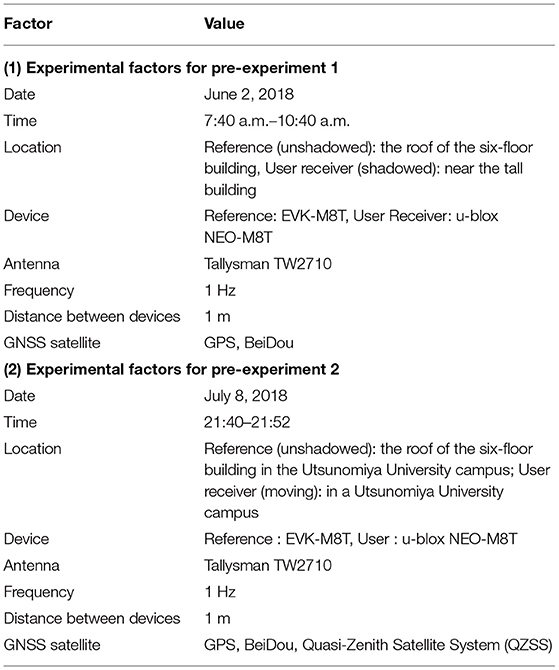
Table 2. Experimental factors for pre-experiment 1 and 2.
In this experiment, true value is defined as the average of the fixed solution. The distance between the two receivers at the unshadowed environment was 0.947 m, whereas that in the shadowed environment was 0.247 m. Since the real distance was 1 m, the result of the shadowed environment was not good. Also, in the unshadowed environment, some epochs do not have an output. Although there were some errors, they were not as severe. Figure 4 (1, 2) shows the error in the shadowed (light color) and unshadowed (dark color) environments at point a, whereas Figure 4 (3, 4) shows the error at point b. If there is no miscalculation, the difference should be 0. The error in the shadowed environment is larger than that in the unshadowed one. The error trend is changing slowly and extensively. From this experiment, we predict that in the shadowed environment, the noise increases. So it may be possible. The shadowed environment has an error by multipath. Also, since the miscalculation trend is changing slowly and significantly in the shadowed environment, we believe that the effect of satellite constellation is more significant than that in the unshadowed environment.
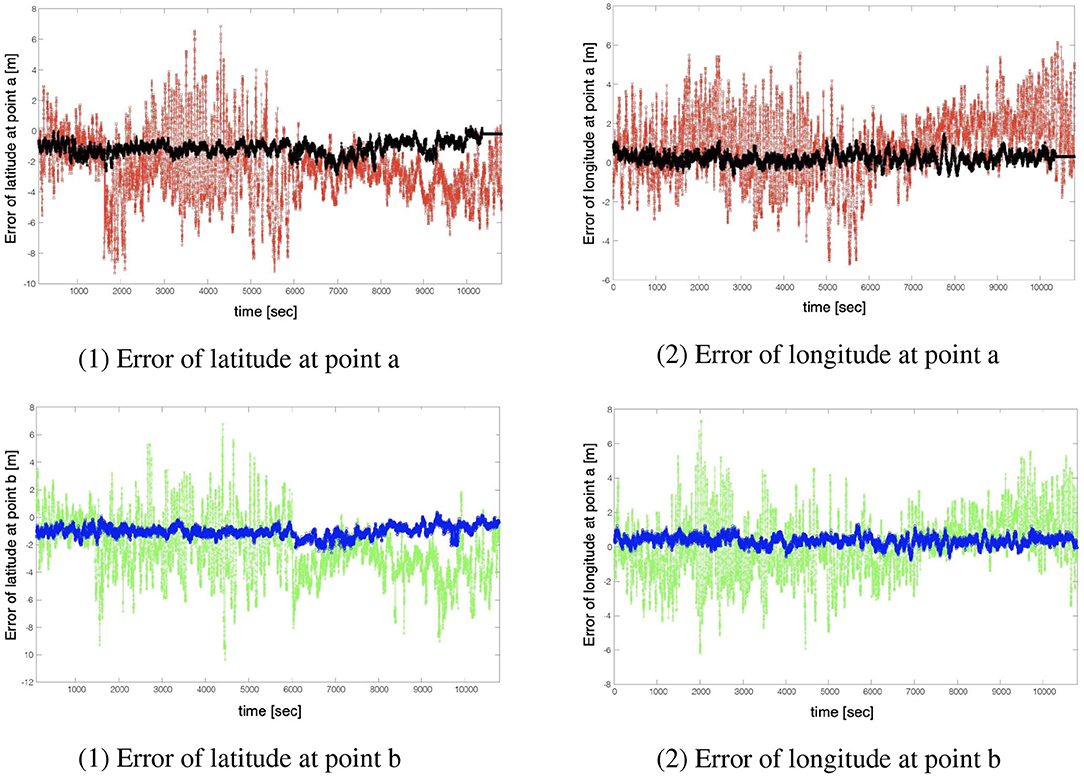
Figure 4. Results at point a and b of pre-experiment 1.
4.2. Evaluating Pre-experiment 2
We performed the next experiment to observe the trend of the positioning results of moving two receivers affected by multipath. We examined the relationship between the average error of the position of each receiver and the distance from the receivers. We set two receivers on a push car, which moved to Utsunomiya University campuses and measured the positions. The distance between receivers was 40 cm. The moving route was selected for motion in the shadowed area. Table 2 (2) shows the experimental factors. We used a fixed RTK solution as the true value and calculated the positioning error as the distance using Hubeny’s formula (Vincenty, 2013) and the longitude and latitude of the receiver’s true value and position.
We define the errors in two receivers as e1 and e2, and the average of the errors is ē=e1+e22[m]. Then, we defined the distance between two receivers as r~[m], as we would like to evaluate the relationship between the average positioning error (ē) and the distance between two receivers (r~). This examination was performed at the epoch, where the positioning error (e1, e2) and distance between receivers (r~) were acquired.
Figure 5 (left) shows how if the distance between receivers (r~) were increased, the average positioning error of two receivers (ē) was increased. Figure 5 (right) is an enlargement of Figure 5 (left), where the distance between receivers (r~) is between 0 and 10 m. This figure shows that there are many points scattered in the positive direction of the vertical axis, but not in the negative direction. Figure 5 (left) and (right) show the distance between receivers (r~) and the average positioning error of two receivers (ē), which has a positive correlation because if ē becomes larger, r~ should be larger.
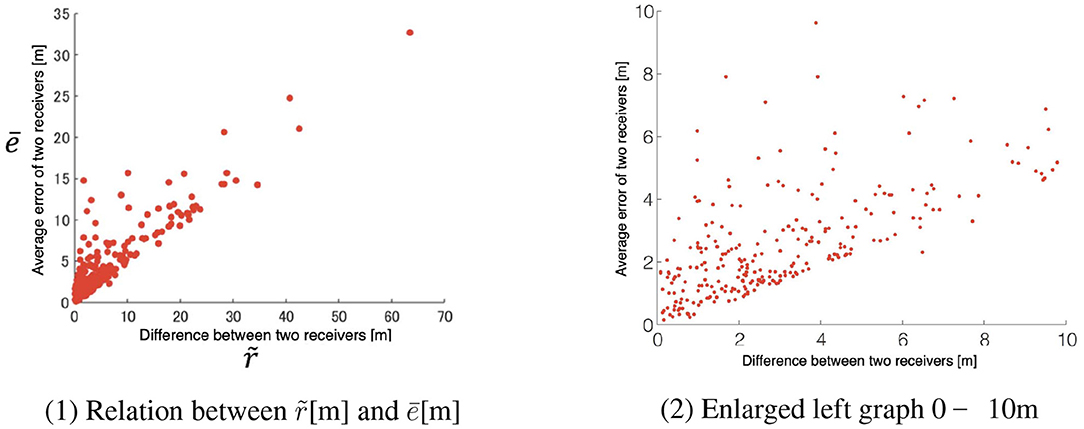
Figure 5. Relationship between the distance of two receivers and the error.
The average positioning error of two receivers (ē) requires the true value, although the distance between receivers (r~) can be calculated from the positioning data of the receiver. Therefore, we believe that it is possible to calculate the average of the positioning error of two receivers (ē) from a distance between receivers (r~) by using two low-cost GNSS receivers. If we can obtain the average of the positioning error of two receivers (ē), we can use that data to develop an error map.
In the next section, we explain the method to calculate the estimated positioning error.
5. The Proposed Method for Calculating the Estimated Positioning Error for the Error Map
This section presents the details of our proposed method for calculating the estimated positioning error for the error map.
5.1. Error Estimation
Figure 6 (1) depicts the parameters and Figure 6 (2) illustrates the system model for the error estimation.
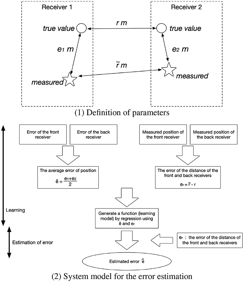
Figure 6. Definition of parameters and System model for the error estimation.
Let us assume there are two receivers located in front of and behind the roof of a car. We use the following parameters:
• e1[m]: positioning error between the true value and the standalone positioning at the front receiver
• e2[m]: positioning error between the true value and the standalone positioning at the back receiver
• r~[m]: the measured distance between two receivers acquired from standalone positioning
• r[m]: the distance between two receivers acquired from the true value
• ē[m]: positioning error of two receivers [calculated by Formula (1)]
• er[m]: error of the distance of two receivers [calculated by Formula (2)].
We obtained the error estimation function by performing a regression analysis, with the front-to-back receiver distance error er since the x-axis and the front-and-back positioning error mean ē as the y-axis. From the shape of Figure 5 (left), we performed linear regression and trained the intercept to become 0. Subsequently, we obtained the relation between er and ē. Using this function, we can obtain er from r~ using Formula (2). We can then estimate ē.
5.2. Deciding on the Magnitude of Error
We discuss the error level evaluation method (i.e., large or small) in this subsection. We also propose methods for deciding on the error level based on the discussion in the previous section. We decide that “the error is large” if the error is larger than r~; otherwise, “the error is small.” However, this simple method sometimes causes an unexpected problem; hence, we would like to discuss this in detail.
5.2.1. Method Using Mileage and Distance Between Positioning Points
The method explained in the previous section has some problems when deciding on the error level. For example, the positioning point receives an error in the same direction and becomes close to the receiver distance’s true value, despite receiving the error. Therefore, the distance calculated from the current time t, the time t′ of the previous epoch, and the speed v are the pseudo-true values. We can then estimate the magnitude of error by taking the difference between the current positioning point and the distance s obtained from the previous epoch’s positioning point [Figure 7 (1)]. This value is the difference between the distance that should have been traveled and the distance that was traveled. Thus, we can decide on this considering the following: the error is large if the value is large, and the error is small if the value is small. Therefore, the problem mentioned at the beginning of this section can be solved in many cases. However, this solution still has issues if the positioning points appear in the vehicle’s opposite direction.
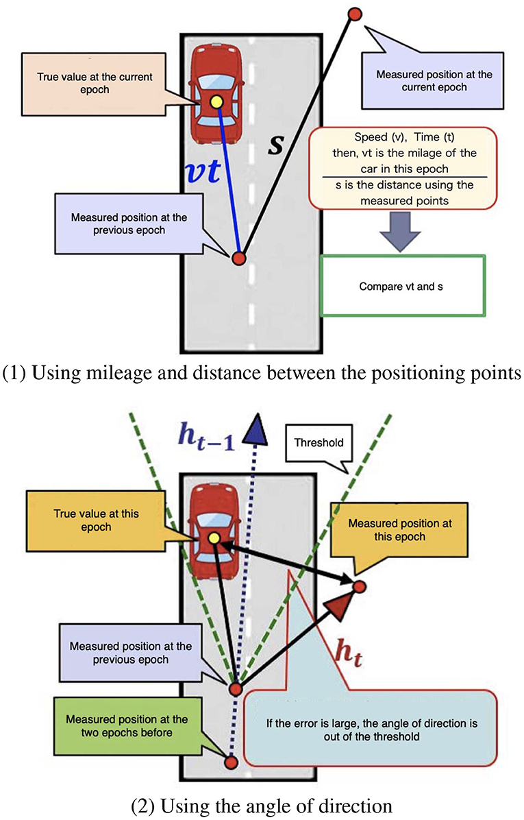
Figure 7. Error level estimation methods.
5.2.2. Method Using the Angle of Direction
We introduce a method for reinforcing the proposed method by using the angle of direction to solve the previous section’s problem. This method is used as an estimation reinforcement when the vehicle is going straight on a straight road. First, the vehicle’s traveling direction angle is obtained using the past two stable positioning points. Next, the threshold of the angle of the vehicle’s traveling direction is set. Finally, we determine if the positioning error is small by determining whether the current epoch’s positioning point is within the threshold of that angle. Figure 7 (2) presents an example. As in the lower-left part, the positioning point of the previous epoch and the vehicle’s traveling direction angle determine whether the current epoch’s positioning point is within the threshold. In this case, it was not within the threshold; thus, it is a “large error.”
5.2.3. Migration of the Methods
We migrate the proposed methods in this section (Figure 8). First, the distance between the two receivers is judged, and we judge whether r~ exceeds 3[m]. If r~>3, we judge this as a “large error.” If r~<3, we judge this as a “small error.” The methods using mileage and angle of the vehicle’s traveling direction are applied. If both methods answer “large error,” the result should be “large error”; otherwise, the result is “small error.”
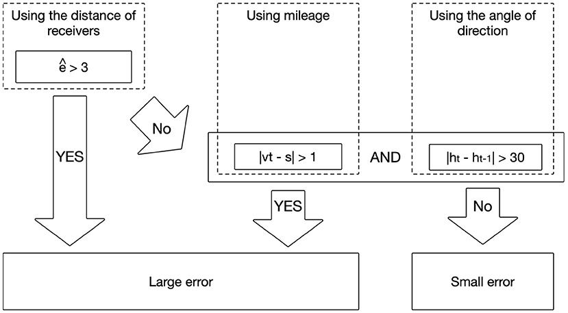
Figure 8. Migration of the methods.
6. Evaluation of the Proposed Methods
This section explains the proposed methods’ evaluation results using a car with two receivers on the roof. The calculation was performed after obtaining the data.
6.1. Evaluation of the Error Estimation Method
Table 3 (1) lists the experiment factors of evaluation of the error estimation method.
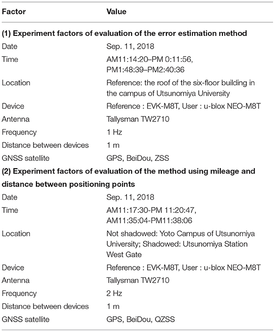
Table 3. Experiment factors of the proposed method.
Two low-priced receivers (u-blox EVK-M8T) were installed on a car roof [Figure 9 (1)]. The distance of the receivers was 1 m. The true value of the position was detected using POS LV 620 from Trimble. POS LV 620 can perform positioning with an accuracy of several centimeters by integrating an inertial measurement unit (IMU) and a DMI (odometer) in addition to a highly accurate GNSS receiver antenna.
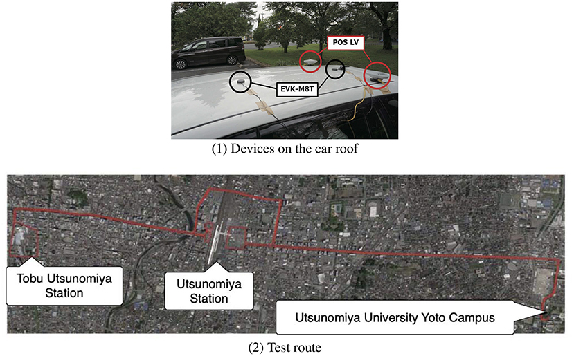
Figure 9. Devices on the car roof and test route.
Figure 9 (2) depicts the route traveled to obtain the experimental data. After leaving Utsunomiya University, Yoto Campus, the car passed through Utsunomiya Station and went to Tobu Utsunomiya Station before returning to Yoto Campus.
The regression analysis data were calculated as the error of the distance of the two receivers (er) and the receiver average positioning error (ē) from the data measured at 1:48:39 p.m.–2:40:36 p.m.. The data used for the evaluation were measured at 11:14:20 a.m.–01: 00: 11: 56 p.m.. We used er of the distance between the front and rear receivers. The error estimation value ẽ output by the function discussed in the previous section was compared with the true value. The estimated positioning error was evaluated for accuracy. The estimated error (ẽ) obtained by the proposed method was subtracted from the positioning error (e1) of the front receiver to obtain the absolute value (i.e., |ê — e1|) summarized as a frequency in Figure 10 (left). Figure 10 (right) depicts a similar result for the back receiver. The value of x = 10 [m] is the frequency, including all 10 m or more errors. The cumulative frequency is also displayed. A comparison of Figure 10 (left) and Figure 10 (right) shows that more than 80% of the estimated error was within 3 m (both within the front and back). Furthermore, in a common part, the epochs with errors of 1 and 2 m are the most in error estimation. The results of Figure 10 (left) are shown in Table 4 as values. The number of epochs is very small when the error is larger than 3 m. The results showed that 80% or more of the estimated error (ẽ) showed an error of 3 m or less from the actual positioning error. We think that the reason for the error of a few meters is the processed regression analysis. The intercept became 0. We also think that no perfect correlation exists in the data, as shown in Figure 5 (left). If the error er in the distance between the front and rear receivers became closer to 0, it became inaccurate in the former case. We think that the reason for this is that the learning process was performed. The intercept became 0. Furthermore, the latter led to the method’s performance degradation because the function’s incompleteness caused it due to the lack of a perfect correlation. This method can also provide a quantitative error amount. Our target was the estimated error of 1 m; however, the result that satisfied this target was approximately 20%. Hence, at this moment, our method is not suitable for a service that requires a strict error level. Our method can be used for services that do not require strict accuracy, such as notifying the user of how reliable the current positioning is.

Figure 10. Frequency of error.
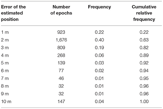
Table 4. Detailed result of frequency of error (front).
6.2. Evaluation of the Method Using Mileage and Distance Between Positioning Points
The evaluation was performed to confirm how much the error can be judged by the proposed method and how much the positioning accuracy can be improved using the «error map.’ We used the same devices that we used in the previous evaluation. Table 3 (2) presents the experiment factors. In this experiment, we prepared two types of cases: one for the shadowed environment and one for the not-shadowed environment. The non-shadowed environment was set up near Utsunomiya University Yoto Campus. This area has a few high shields to the left and right of the road, and a stable positioning is possible. The shadowed environment was set up at the rotary at the west exit of Utsunomiya Station. There are many tall buildings around this area, and a pedestrian bridge covers the zenith direction. The evaluation was performed by using the method for determining the magnitude of the error and comparing it with the magnitude of the front receiver’s actual error amount. After determining the magnitude of the error using this method, we confirmed whether the positioning accuracy could be improved by selecting satellites using the elevation mask. In the case of a “large error,” we predicted the positioning accuracy could be improved by selecting a high-elevation satellite that does not cause a multi-path. In the case of a “small error,” we predicted the positioning accuracy could be improved by using more satellites in such a way that the weak elevation mask would be useful. We want to verify the error map effectiveness. Table 5 (1) describes the result of the non-shadowed environment. The success rate of the judgment was 97.6%. The result showed that the error size was successfully judged with high accuracy. Almost all actual errors showed a “small error” in the epoch, which is the reason why the judgment was performed well by the method. Table 5 (2) describes the results of the shadowed environment. The judgment success rate was 72.1%, which was not highly accurate. We verified to what extent the elevation mask effect was obtained with this success rate. To calculate the positioning error, we set the elevation mask to 15° (general elevation mask value) when the judgment was “small error” and to 30° when the judgment was “large error.” The results were then compared to those when the mask was set to 15° all the time.
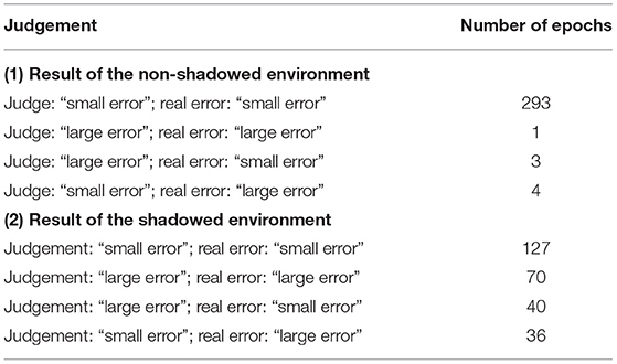
Table 5. Results of evaluation of the method using mileage and distance between positioning points.
The average positioning error of fixed elevation mask (15°) was 5.78 m, and that of variable elevation mask was 5.50 m. This result shows that when the elevation mask was adjusted according to the judgment result, the average positioning error was improved by approximately 0.3 m compared to when the elevation mask was always set to the same value of 15°. By applying this method, the positioning accuracy was improved for 59.5% of the epoch. The loss of six of 273 epochs can be prevented compared to when the elevation mask was always set to 15°. In the non-shadowed environment, the error size was successfully discriminated by the method, and the discrimination was very high at 97.6%. However, in the shadowed environment, the discrimination was at 72.1%. In this environment, the judgment’s success rate decreased because the parts discriminated against as “small error” and as “large error” were mixed. However, as a result of setting the elevation mask using this judgment result, we confirmed that the positioning accuracy was improved, albeit with a small value of 0.3 m. The positioning accuracy did not improve much because only a few epochs can significantly improve 1 m or more when the 15° and 30° elevation masks were applied. Therefore, we believe that a great effect can be expected in an environment where the positioning accuracy can be greatly improved by adjusting the elevation mask. Moreover, distinguishing between regions where positioning is stable and where it is unstable is possible. Hence, this method can be used to construct an error map.
The estimation error method could be used to estimate the positioning error. However, a precise error amount cannot be obtained; therefore, we need to select a service that can use this method. We also confirmed that the method using mileage and distance between positioning points could be used for the magnitude of error judgment, especially in the non-shadowed environment, and displays a high error judgment rate. On the contrary, the judgment accuracy in the shadowed environment was lower. We evaluated the effect of changing the elevation masks using the result. Consequently, we confirmed that the error can be improved, albeit insignificantly.
7. Possible Error Map Applications
We discuss the possibility of the error map application in this section.
7.1. A-GPS
Assisted GPS (A-GPS) is a technology that uses information from base stations for positioning with mobile phones. A-GPS is useful for roughly grasping the user position from the received signal base station and narrowing down the user position. A technology called place engine performs positioning using Wi-Fi access points, even in indoor positioning, where satellite signals cannot be received. Therefore, in a shadowed environment, the positioning accuracy can be expected to improve by installation (e.g., beacons). For this purpose, a database of location information must be developed as an infrastructure. An error map can be used as a guide for setting up such infrastructure.
7.2. Elevation Mask Adjustment
We discussed this technique in the previous section. Satellites with low elevation angles generally often transmit low-quality signals. A receiver usually has a function that eliminates satellites transmitting low-quality signals by referring to the elevation angle. If the error map is used to estimate the “small error,” the result is used to apply a weak elevation mask. Consequently, the overall accuracy of the positioning could be increased.
7.3. RTK
RTK is one of the technologies that has been drawing attention in recent years. It is a method of obtaining a mobile station’s coordinates by finding the relative position with the mobile station on the user side by employing a reference station whose coordinates are known. The method accuracy is said to be of the order of a few centimeters, and high positioning accuracy can be achieved. The RTK system is required to count the number of satellite carrier waves at the user receiver. However, they may be interrupted by blocking the signal at a shadow, such as a building. Consequently, positioning may not be stable, even if the RTK is used in a shadowed environment. The degradation of the RTK positioning accuracy can be prevented by eliminating a satellite with a low-quality signal. It is possible to determine whether the environment is shadowed or not by using an error map; thus, it is possible to improve the positioning accuracy by using the variable elevation mask described to eliminate satellites that may cause signal interruptions.
7.4. Dynamic Map
Current positioning systems often use sensors to perform highly accurate positioning. Positioning support using dynamic maps for transportation is expected as a support method. Technologies that use map information, such as map matching, are often used. A system that supports each user’s positioning should be put to practical use by employing the map information and the 3D building information, and smartphone and automobile information as big data. In this study, we examined the method for making a GNSS positioning error map as part of such a dynamic map. Furthermore, using 5G is expected to increase the communication speed, reduce the hardware size of IoT systems, and improve the data mining technology to enable an efficient use of big data. We expect the availability of dynamic maps in the future.
8. Conclusion
In this paper, we mentioned a cognitive navigation system inspired by the CogInfoCom that extends human cognitive capabilities and would even enable life support. Also, we described details of the error map as the technical basis of a cognitive navigation system.
An error map was designed to display the accuracy of the positioning of GNSS. We mentioned the method to measure the positioning error of GNSS by using two GNSS receivers. We designed the technique in two ways using two GNSS receivers, namely the estimation of error using two GNSS receivers and the comparison of the error size assisted by the error map. First, we explained the problems related to positioning using GNSS and proposed the new error map idea to adopt the multi-path environment and acquire a better position result. Next, we investigated the positioning error caused by the multi-path under a shadowed environment when moving and stopping. Consequently, we confirmed that the distance of the two GNSS receivers and the average positioning error from these two receivers positively correlate. We proposed the two following methods according to the results: (1) error estimation by the linear regression; and (2) comparison of the error size assisted by the error map. We then evaluated the performance of the proposed method.
It is difficult to estimate the level of positioning error of GNSS. Usually, the number of satellites or Dilution of Precision (DOP) is used for that purpose. However, such methods cannot estimate the level of the error caused by multipath by buildings. A new idea to estimate the level of positioning error of GNSS is required by reflecting real filed positioning data. The proposed idea provides a useful and straightforward method to estimate the level of positioning error of GNSS by using a known distance of two GNSS receives.
Our method satisfied the target (error ≦ 1 m) of 20% of test data, but could not satisfy the target we set in sections 4 and 5. However, we can use our method for LBS, which does not require a critical boundary of accuracy. For the error size comparison, the no-shadow case provided an accuracy of over 90%; however, the accuracy was lower than 72% in the shadow case. We can distinguish the positioning stability; thus, we can offer a service to provide information about the possible error by using the error map and develop LBSs by incorporating the location’s possible error.
The development of a real error map requires further study. If we develop an error map, we should consider several things, including the useful number of error levels (such as 3 or 5 or 10) and the number of epochs for error calculation. Also, the idea of developing and maintaining the error map is required. One possibility is to attach GNSS receivers on buses, trucks, and taxis to collect the position data and errors. The map must be frequently updated after developing the error map. This map provides information about the error level, and the user can rely on it as information to support positioning (e.g., shadow mask application to obtain more accurate position data or understand the position data reliability).
We think that many fields can be extended usability and performance by using the idea of CogInfoCom. We would like to try to use the concept of CogInfoCom in the different research areas.
Data Availability Statement
The raw data supporting the conclusions of this article will be made available by the authors, without undue reservation.
Author Contributions
All authors listed have made a substantial, direct and intellectual contribution to the work, and approved it for publication.
Funding
The part of the research results was obtained from the commissioned research by the National Institute of Information and Communications Technology (NICT), JAPAN. Also, this research was supported by JSPS KAKENHI Grant Number JP17H02249, JP18K11849, and JP17H01731.
Conflict of Interest
The authors declare that the research was conducted in the absence of any commercial or financial relationships that could be construed as a potential conflict of interest.
References
Baranyi, P., and Csapo, A. (2012). Definition and synergies of cognitive infocommunications. Acta Polytech. Hung. 9, 67–83.
Google Scholar
Baranyi, P., Csapo, A., and Sallai, G. (2015). Cognitive Infocommunications (CogInfoCom). Cham: Springer International.
Google Scholar
Iwase, T., Suzuki, N., and Watanabe, Y. (2013). Estimation and exclusion of multipath range error for robust positioning. GPS Solut. 17, 53–62. doi: 10.1007/s10291-012-0260-1
CrossRef Full Text | Google Scholar
Kitani, T., Hatano, H., Onishi, H., and Hirao, S. (2012). A Method to Improve Positioning Accuracy of GPS by Sharing Error Information Among Neighbor Devices. Information Processing Society of Japan SIG Technical Report in Japanese 2012-ITS-49, 1–6.
Klobuchar, J. A. (1987). Ionospheric time-delay algorithm for single frequency GPS users. IEEE Trans. Aerospace Electr. Syst. 23, 325–331. doi: 10.1109/TAES.1987.310829
CrossRef Full Text | Google Scholar
Kubo, N., Kobayashi, K., Hsu, L.-T., and Amai, O. (2017). Multipath mitigation technique under strong multipath environment using multiple antennas. J. Aeronaut. 49, 75–82.
Google Scholar
Misra, P., and Enge, P. (2001). Global Positioning System Signals, Measurements, and Performance. Lincoln, MA: Ganga-Jamuna Press.
PubMed Abstract | Google Scholar
Miyata, H., Noguchi, T., Sakitani, A., and Egashira, S. (1996). Consideration on high accurate positioning with simplified DGPS. ITE Tech. Rep. (in Japanese) 20, 71–76.
Miyata, H., and Sakitani, A. (1997). Improving accuracy of simplified dgps positioning by the after processing. ITE Tech. Rep. (in Japanese) 21, 19–22.
Nakamura, Y. (2018). A research on reduction method of positioning error based on error characteristics under the same combination of gnss satellites. Utsunomiya: Utsunomiya University Graduation thesis (in Japanese).
Odaka, Y., Takano, S., In, Y., Higuchi, M., and Murakami, H. (2011). “The evaluation of the error characteristics of multiple GPS terminals,” in Proceedings of the 2nd International Conference on Circuits, Systems, Control, Signals (CSCS ’11) (Prague), 13–21.
Google Scholar
Osechas, O., Kim, K. J., Parsons, K., and Sahinoglu, Z. (2015). “Detecting multipath errors in terrestrial GNSS applications,” in Proceedings of the 2015 International Technical Meeting of The Institute of Navigation (Dana Point, CA), 465–474.
Google Scholar
Rohani, M., Gingras, D., and Gruyer, D. (2016). A novel approach for improved vehicular positioning using cooperative map matching and dynamic base station DGPS concept. IEEE Trans. Intell. Transport. Syst. 17, 230–239. doi: 10.1109/TITS.2015.2465141
CrossRef Full Text | Google Scholar
Saastamoinen, J. (1973a). Contributions to the theory of atmospheric refraction. Bull. Geodesique 30, 279–298.
Google Scholar
Saastamoinen, J. (1973b). Contributions to the theory of atmospheric refraction. Bull. Geodesique 30, 383–397.
Google Scholar
Saastamoinen, J. (1973c). Contributions to the theory of atmospheric refraction. Bull. Geodesique 30, 13–34.
Google Scholar
Sakai, T. (2003). Introduction of GPS. Tokyo: Tokyo Denki University Press.
Satirapod, C., and Chalermwattanachai, P. (2005). Impact of different tropospheric models on gps baseline accuracy: case study in Thailand. J. Glob. Posit. Syst. 4, 36–40. doi: 10.5081/jgps.4.1.36
CrossRef Full Text | Google Scholar
Vincenty, T. (2013) (1975 (Published online: 2013)). Direct and inverse solutions of geodesics on the ellipsoid with application of nested equations. Surv. Rev. XXIII, 88–93. doi: 10.1179/sre.1975.23.176.88.
CrossRef Full Text | Google Scholar
Watanabe, Y., Sato, K., and Takada, H. (2020). Dynamicmap 2.0: a traffic data management platform leveraging clouds, edges and embedded systems. Int. J. Intell. Transport. Syst. Res. 18, 77–89. doi: 10.1007/s13177-018-0173-7
CrossRef Full Text | Google Scholar
GPS pseudorange and carrier-phase measurements are both affected by several types of random errors and biases (systematic errors). These errors may be classified as those originating at the satellites, those originating at the receiver, and those that are due to signal propagation (atmospheric refraction) [1]. Figure 3.1 shows the various errors and biases.
The errors originating at the satellites include ephemeris, or orbital, errors, satellite clock errors, and the effect of selective availability. The latter was intentionally implemented by the U.S. DoD to degrade the autonomous GPS accuracy for security reasons. It was, however, terminated at midnight (eastern daylight time) on May 1, 2000 [2]. The errors originating at the receiver include receiver clock errors, multipath error, receiver noise, and antenna phase center variations. The signal propagation errors include the delays of the GPS signal as it passes through the ionospheric and tropospheric layers of the atmosphere. In fact, it is only in a vacuum (free space) that the GPS signal travels, or propagates, at the speed of light.
In addition to the effect of these errors, the accuracy of the computed GPS position is also affected by the geometric locations of the GPS satellites as seen by the receiver. The more spread out the satellites are in the sky, the better the obtained accuracy (Figure 3.1).

Figure 3.1 GPS errors and biases.
For example, combining L1 and L2 observables removes, to a high degree of accuracy, the effect of the ionosphere. Mathematical modeling of these errors and biases is also possible. In this topic, the main GPS error sources are introduced and the ways of treating them are discussed.
GPS ephemeris errors
Satellite positions as a function of time, which are included in the broadcast satellite navigation message, are predicted from previous GPS observations at the ground control stations. Typically, overlapping 4-hour GPS data spans are used by the operational control system to predict fresh satellite orbital elements for each 1-hour period. As might be expected, modeling the forces acting on the GPS satellites will not in general be perfect, which causes some errors in the estimated satellite positions, known as ephemeris errors. Nominally, an ephemeris error is usually in the order of 2m to 5m, and can reach up to 50m under selective availability [3]. According to [2], the range error due to the combined effect of the ephemeris and the satellite clock errors is of the order of 2.3m [1s-level; s is the standard deviation.
An ephemeris error for a particular satellite is identical to all GPS users worldwide [4]. However, as different users see the same satellite at different view angles, the effect of the ephemeris error on the range measurement, and consequently on the computed position, is different. This means that combining (differencing) the measurements of two receivers simultaneously tracking a particular satellite cannot totally remove the ephemeris error. Users of short separations, however, will have an almost identical range error due to the ephemeris error, which can essentially be removed through differencing the observations. For relative positioning,the following rule of thumb gives a rough estimate of the effect of the ephemeris error on the baseline solution: the baseline error / the baseline length = the satellite position error / the range satellite [5]. This means that if the satellite position error is 5m and the baseline length is 10 km, then the expected baseline line error due to ephemeris error is approximately 2.5 mm.
Some applications, such as studies of the crustal dynamics of the earth, require more precise ephemeris data than the broadcast ephemeris. To support these applications, several institutions [e.g., the International GPS Service for Geodynamics (IGS), the U.S. National Geodetic Survey (NGS), and Geomatics Canada] have developed postmission precise orbital service. Precise ephemeris data is based on GPS data collected at a global GPS network coordinated by the IGS. At the present time, precise ephemeris data is available to users with some delay, which varies from 12 hours for the IGS ultra rapid orbit to about 12 days for the most precise IGS precise orbit. The corresponding accuracies for the two precise orbits are in the order of a few decimeters to 1 decimeter, respectively. Users can download the precise ephemeris data free of charge from the IGS center, at ftp://igscb.jpl.nasa.gov/igscb/product/.
Selective availability
GPS was originally designed so that real-time autonomous positioning and navigation with the civilian C/A code receivers would be less precise than military P-code receivers. Surprisingly, the obtained accuracy was almost the same from both receivers. To ensure national security, the U.S. DoD implemented the so-called selective availability (SA) on Block II GPS satellites to deny accurate real-time autonomous positioning to unauthorized users. SA was officially activated on March 25, 1990 [3].
SA introduces two types of errors [6]. The first one, called delta error, results from dithering the satellite clock, and is common to all users worldwide. The second one, called epsilon error, is an additional slowly varying orbital error. With SA turned on, nominal horizontal and vertical errors can be up to 100m and 156m, respectively, at the 95% probability level. Figure 3.2 shows how the horizontal position of a stationary GPS receiver varies over time, mainly as a result of the effect of SA. Like the range error due to ephemeris error, the range error due to epsilon error is almost identical between users of short separations. Therefore, using differential GPS would overcome the effect of the epsilon error. In fact, DGPS provides better accuracy than the standalone P-code receiver due to the elimination or the reduction of the common errors, including SA [4].
Following extensive studies, the U.S. government discontinued SA on May 1,2000, resulting in a much-improved autonomous GPS accuracy [2]. With the SA turned off, the nominal autonomous GPS horizontal and vertical accuracies would be in the order of 22m and 33m (95% of the time), respectively.

Figure 3.2 Position variation of a stationary GPS receiver due to SA.
Figure 3.3 shows the GPS errors after SA was turned off. The elimination of SA will open the door for faster growth of GPS markets (e.g., vehicle navigation and enhanced-911). Although the removal of SA would have little impact on the DGPS accuracy, it would reduce the cost of installing and operating a DGPS system. This is mainly because of the reduction in the required transmission rate.
Satellite and receiver clock errors
Each GPS Block II and Block IIA satellite contains four atomic clocks, two cesium and two rubidium [7]. The newer generation Block IIR satellites carry rubidium clocks only. One of the onboard clocks, primarily a cesium for Block II and IIA, is selected to provide the frequency and the timing requirements for generating the GPS signals. The others are backups [7].
The GPS satellite clocks, although highly accurate, are not perfect. Their stability is about 1 to 2 parts in 1013 over a period of one day. This means that the satellite clock error is about 8.64 to 17.28 ns per day. The corresponding range error is 2.59m to 5.18m, which can be easily calculated by multiplying the clock error by the speed of light (i.e., 299,729,458 m/s). Cesium clocks tend to behave better over a longer period of time compared with rubidium clocks. In fact, the stability of the cesium clocks over a period of 10 days or more improves to several parts in 1014 [7].

Figure 3.3 Position variation of a stationary GPS receiver after terminating SA.
The performance of the satellite clocks is monitored by the ground control system. The amount of drift is calculated and transmitted as a part of the navigation message in the form of three coefficients of a second-degree polynomial [3, 8].
Satellite clock errors cause additional errors to the GPS measurements. These errors are common to all users observing the same satellite and can be removed through differencing between the receivers. Applying the satellite clock correction in the navigation message can also correct the satellite clock errors. This, however, leaves an error of the order of several nanoseconds, which translates to a range error of a few meters (one nanosecond error is equivalent to a range error of about 30 cm) [4].
GPS receivers, in contrast, use inexpensive crystal clocks, which are much less accurate than the satellite clocks [1]. As such, the receiver clock error is much larger than that ofthe GPS satellite clock. It can, however, be removed through differencing between the satellites or it can be treated as an additional unknown parameter in the estimation process. Precise external clocks (usually cesium or rubidium) are used in some applications instead of the internal receiver clock. Although the external atomic clocks have superior performance compared with the internal receiver clocks, they cost between a few thousand dollars for the rubidium clocks to about $20,000 for the cesium clocks.
Multipath error
Multipath is a major error source for both the carrier-phase and pseu-dorange measurements. Multipath error occurs when the GPS signal arrives at the receiver antenna through different paths [5]. These paths can be the direct line of sight signal and reflected signals from objects surrounding the receiver antenna (Figure 3.4).
Multipath distorts the original signal through interference with the reflected signals at the GPS antenna. It affects both the carrier-phase and pseudorange measurements; however, its size is much larger in the pseu-dorange measurements. The size of the carrier-phase multipath can reach a maximum value of a quarter of a cycle (about 4.8 cm for the L1 carrier phase). The pseudorange multipath can theoretically reach several tens of meters for the C/A-code measurements. However, with new advances in receiver technology, actual pseudorange multipath is reduced dramatically.

Figure 3.4 Multipath effect.
Examples of such technologies are the Strobe correlator (Ashtech, Inc.) and the MEDLL (NovAtel, Inc.). With these multipath-mitigation techniques, the pseudorange multipath error is reduced to several meters, even in a highly reflective environment [9].
Under the same environment, the presence of multipath errors can be verified using a day-to-day correlation of the estimated residuals [3]. This is because the satellite-reflector-antenna geometry repeats every sidereal day. However, multipath errors in the undifferenced pseudorange measurements can be identified if dual-frequency observations are available. A good general multipath model is still not available, mainly because of the variant satellite-reflector-antenna geometry. There are, however, several options to reduce the effect of multipath. The straightforward option is to select an observation site with no reflecting objects in the vicinity of the receiver antenna. Another option to reduce the effect of multipath is to use a chock ring antenna (a chock ring device is a ground plane that has several concentric metal hoops, which attenuate the reflected signals). As the GPS signal is right-handed circularly polarized while the reflected signal is left-handed, reducing the effect of multipath may also be achieved by using an antenna with a matching polarization to the GPS signal (i.e., right-handed). The disadvantage of this option, however, is that the polarization of the multipath signal becomes right-handed again if it is reflected twice [9].
Antenna-phase-center variation
The point at which the GPS signal is received is called the antenna phase center [3]. Generally, the antenna phase center does not coincide with the physical (geometrical) center of the antenna. It varies depending on the elevation and the azimuth of the GPS satellite as well as the intensity of the observed signal. As a result, additional range error can be expected [3].
The size of the error caused by the antenna-phase-center variation depends on the antenna type, and is typically in the order of a few centimeters. It is, however, difficult to model the antenna-phase-center variation and, therefore, care has to be taken when selecting the antenna type [1]. For short baselines with the same types of antennas at each end, the phase-center error can be canceled if the antennas are oriented in the same direction [11]. Mixing different types of antennas or using different orientations will not cancel the error. Due to its rather small size, this error is neglected in most of the practical GPS applications.
It should be pointed out that phase-center errors could be different on L1 and L2 carrier-phase observations. This can affect the accuracy of the ionosphere free linear combination, particularly when observing short baselines. As mentioned before, for short baselines, the errors are highly correlated over distance and cancel sufficiently through differencing. Therefore, using a single frequency might be more appropriate for short baselines in the static mode.