#VALUE is Excel’s way of saying, «There’s something wrong with the way your formula is typed. Or, there’s something wrong with the cells you are referencing.» The error is very general, and it can be hard to find the exact cause of it. The information on this page shows common problems and solutions for the error. You may need to try one or more of the solutions to fix your particular error.

Fix the error for a specific function
Don’t see your function in this list? Try the other solutions listed below.
Problems with subtraction
If you’re new to Excel, you might be typing a formula for subtraction incorrectly. Here are two ways to do it:
Subtract a cell reference from another
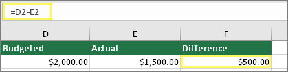
Type two values in two separate cells. In a third cell, subtract one cell reference from the other. In this example, cell D2 has the budgeted amount, and cell E2 has the actual amount. F2 has the formula =D2-E2.
Or, use SUM with positive and negative numbers
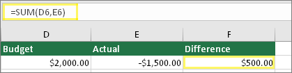
Type a positive value in one cell, and a negative value in another. In a third cell, use the SUM function to add the two cells together. In this example, cell D6 has the budgeted amount, and cell E6 has the actual amount as a negative number. F6 has the formula =SUM(D6,E6).
If you’re using Windows, you might get the #VALUE! error when doing even the most basic subtraction formula. The following might solve your problem:
-
First do a quick test. In a new workbook, type a 2 in cell A1. Type a 4 in cell B1. Then in C1 type this formula =B1-A1. If you get the #VALUE! error, go to the next step. If you don’t get the error, try other solutions on this page.
-
In Windows, open your Region control panel.
-
Windows 10: Click Start, type Region, and then click the Region control panel.
-
Windows 8: At the Start screen, type Region, click Settings, and then click Region.
-
Windows 7: Click Start and then type Region, and then click Region and language.
-
-
On the Formats tab, click Additional settings.
-
Look for the List separator. If the List separator is set to the minus sign, change it to something else. For example, a comma is a common list separator. The semicolon is also common. However, another list separator might be more appropriate for your particular region.
-
Click OK.
-
Open your workbook. If a cell contains a #VALUE! error, double-click to edit it.
-
If there are commas where there should be minus signs for subtraction, change them to minus signs.
-
Press ENTER.
-
Repeat this process for other cells that have the error.
Subtract a cell reference from another
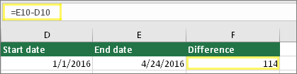
Type two dates in two separate cells. In a third cell, subtract one cell reference from the other. In this example, cell D10 has the start date, and cell E10 has the End date. F10 has the formula =E10-D10.
Or, use the DATEDIF function
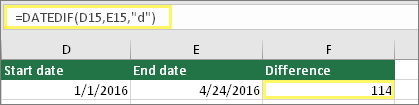
Type two dates in two separate cells. In a third cell, use the DATEDIF function to find the difference in dates. For more information on the DATEDIF function, see Calculate the difference between two dates.
Make your date column wider. If your date is aligned to the right, then it’s a date. But if it’s aligned to the left, this means the date isn’t really a date. It’s text. And Excel won’t recognize text as a date. Here are some solutions that can help this problem.
Check for leading spaces
-
Double-click a date that is being used in a subtraction formula.
-
Put your cursor at the beginning and see if you can select one or more spaces. Here’s what a selected space looks like at the beginning of a cell:

If your cell has this problem, proceed to the next step. If you don’t see one or more spaces, go to the next section on checking your computer’s date settings.
-
Select the column that contains the date by clicking its column header.
-
Click Data > Text to Columns.
-
Click Next twice.
-
On Step 3 of 3 of the wizard, under Column data format, click Date.
-
Choose a date format, and then click Finish.
-
Repeat this process for other columns to ensure they don’t contain leading spaces before dates.

Check your computer’s date settings
Excel uses your computer’s date system. If a cell’s date isn’t entered using the same date system, then Excel won’t recognize it as a true date.
For example, let’s say that your computer displays dates as mm/dd/yyyy. If you typed a date like that in a cell, Excel would recognize it as a date and you’d be able to use it in a subtraction formula. However, if you typed a date like dd/mm/yy, then Excel wouldn’t recognize that as a date. Instead, it would treat it as text.
There are two solutions to this problem: You could change the date system that your computer uses to match the date system you want to type in Excel. Or, in Excel you could create a new column and use the DATE function to create a true date based on the date stored as text. Here’s how to do that assuming your computers date system is mm/dd/yyy and your text date is 31/12/2017 in cell A1:
-
Create a formula like this: =DATE(RIGHT(A1,4),MID(A1,4,2),LEFT(A1,2))
-
The result would be 12/31/2017.
-
If you want the format to appear like dd/mm/yy, press CTRL+1 (or
+ 1 on the Mac). -
Choose a different locale that uses the dd/mm/yy format, for example, English (United Kingdom). When you’re done applying the format, the result would be 31/12/2017 and it would be a true date, not a text date.
 + 1 on the Mac).
Note: The formula above is written with the DATE, RIGHT, MID, and LEFT functions. Please notice that it is written with an assumption that the text date has two characters for days, two characters for months, and four characters for year. You may need to customize the formula to suit your date.
Problems with spaces and text
Often #VALUE! occurs because your formula refers to other cells that contain spaces, or even trickier: hidden spaces. These spaces can make a cell look blank, when in fact they are not blank.
1. Select referenced cells
Find cells that your formula is referencing and select them. In many cases removing spaces for an entire column is a good practice because you can replace more than one space at a time. In this example, clicking the E selects the entire column.
2. Find and replace

On the Home tab, click Find & Select > Replace.
3. Replace spaces with nothing
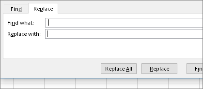
In the Find what box, type a single space. Then, in the Replace with box, delete anything that might be there.
4. Replace or Replace all
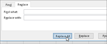
If you are confident that all spaces in the column should be removed, click Replace All. If you’d like to step through and replace spaces with nothing on an individual basis, you can click Find next first, and then click Replace when you are confident the space isn’t needed. When you’re done, the #VALUE! error may be resolved. If not, go to the next step.
5. Turn on the filter
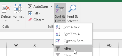
Sometimes there are hidden characters other than spaces that can make a cell appear blank, when it’s not really blank. Single apostrophes within a cell can do this. To get rid of these characters in a column, turn on the filter by going to Home > Sort & Filter > Filter.
6. Set the filter

Click the filter arrow  , and then deselect Select all. Then, select the Blanks checkbox.
7. Select any unnamed checkboxes
Select any check boxes that don’t have anything next to them, like this one.
8. Select blank cells, and delete

When Excel brings back the blank cells, select them. Then press the Delete key. This will clear any hidden characters in the cells.
9. Clear the filter
Click the filter arrow , and then click Clear filter from… so that all cells are visible.
10. Result
If spaces were the culprit of your #VALUE! error then hopefully your error has been replaced by the formula result, as shown here in our example. If not, repeat this process for other cells that your formula refers to. Or, try other solutions on this page.
Note: In this example, notice that cell E4 has a green triangle and the number is aligned to the left. This means the number is stored as text. This may cause more problems later. If you see this problem, we recommend converting numbers stored as text to numbers.
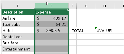
Text or special characters within a cell can cause the #VALUE! error. But sometimes it’s hard to see which cells have these problems. Solution: Use the ISTEXT function to inspect cells. Please note that ISTEXT doesn’t resolve the error, it simply finds cells that might be causing the error.
Example with #VALUE!
Here’s an example of a formula that has a #VALUE! error. This is likely due to cell E2. There is a special character that appears as a small box after «00.» Or as the next picture shows, you could use the ISTEXT function in a separate column to check for text.
Same example, with ISTEXT
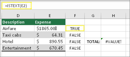
Here the ISTEXT function was added in column F. All cells are fine except the one with the value of TRUE. This means cell E2 has text. To resolve this, you could delete the cell’s contents and retype the value of 1865.00. Or you could also use the CLEAN function to clean out characters, or use the REPLACE function to replace special characters with other values.
After using CLEAN or REPLACE, you’ll want to copy the result, and use Home > Paste > Paste Special > Values. You might also have to convert numbers stored as text to numbers.
Formulas with math operations like + and * may not be able to calculate cells that contain text or spaces. In this case, try using a function instead. Functions will often ignore text values and calculate everything as numbers, eliminating the #VALUE! error. For example, instead of =A2+B2+C2, type =SUM(A2:C2). Or, instead of =A2*B2, type =PRODUCT(A2,B2).
Other solutions to try
Select the error

First select the cell with the #VALUE! error.
Click Formulas > Evaluate Formula
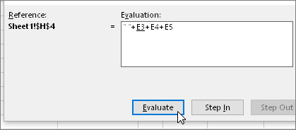
Click Formulas > Evaluate Formula > Evaluate. Excel will step through the parts of the formula individually. In this case the formula =E2+E3+E4+E5 breaks because of a hidden space in cell E2. You can’t see the space by looking at cell E2. However, you can see it here. It shows as » «.
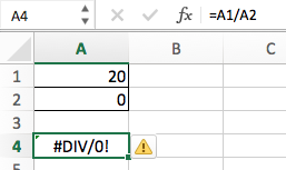
Sometimes you just want to replace the #VALUE! error with something else like your own text, a zero or a blank cell. In this case you can add the IFERROR function to your formula. IFERROR will check to see if there’s an error, and if so, replace it with another value of your choice. If there isn’t an error, your original formula will be calculated. IFERROR will only work in Excel 2007 and later. For earlier versions you can use IF(ISERROR()).
Warning: IFERROR will hide all errors, not just the #VALUE! error. Hiding errors isn’t recommended because an error is often a sign that something needs to be fixed, not hidden. We don’t recommend using this function unless you are absolutely certain your formula works the way that you want.
Cell with #VALUE!
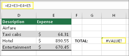
Here’s an example of a formula that has a #VALUE! error due to a hidden space in cell E2.
Error hidden by IFERROR
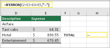
And here’s the same formula with IFERROR added to the formula. You can read the formula as: «Calculate the formula, but if there’s any kind of error, replace it with two dashes.» Note that you could also use «» to display nothing instead of two dashes. Or you could substitute your own text, such as: «Total Error».
Unfortunately, you can see that IFERROR doesn’t actually resolve the error, it simply hides it. So be certain that hiding the error is better than fixing it.
Your data connection may have become unavailable at some point. To fix this, restore the data connection, or consider importing the data if possible. If you don’t have access to the connection, ask the creator of the workbook to make a new file for you. The new file ideally would only have values, and no connections. They can do this by copying all the cells, and pasting only as values. To paste as only values, they can click Home > Paste > Paste Special > Values. This eliminates all formulas and connections, and therefore would also remove any #VALUE! errors.
See Also
Overview of formulas in Excel
How to avoid broken formulas
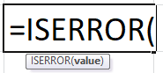
ISERROR is a logical function that is used to identify whether the cells being referred to have an error or not. This function identifies all the mistakes. If any error is found in the cell, it returns “TRUE” as a result, and if the cell has no errors, it gives “FALSE” as a result. This function takes a cell reference as an argument.
ISERROR function in Excel checks if any given expression returns an error in Excel.
For example, suppose you have a dataset and applied the ISERROR formula to divide the number by 0. In such a scenario, the ISERROR Excel function verifies the value and returns ” TRUE” if it possesses an error. Therefore, Excel displays the #DIV/0! Error. Conversely, as a result, it provides ” FALSE” if it does not consist of any error.
Table of contents
- ISERROR Function in Excel
- ISERROR Formula in Excel
- Arguments used for ISERROR Function.
- Returns
- ISERROR in Excel – Illustration
- How to Use the ISERROR Function in Excel?
- ISERROR in Excel Example #1
- ISERROR in Excel Example #2
- ISERROR in Excel Example #3
- Things to Know about the ISERROR Function in Excel
- ISERROR Excel Function Video
- Recommended Articles
- ISERROR Formula in Excel
ISERROR Formula in Excel
Arguments used for ISERROR Function.
Value: The expression or value to be tested for error.
The value can be a number, text, mathematical operation, or expression.
Returns
The output of ISERROR in Excel is a logical expression. If the supplied argument gives an error in Excel, it returns “TRUE.” Otherwise, it returns “FALSE.” For error messages- #N/A, #VALUE!, #REF!, #DIV/0!, #NUM!, #NAME?, and #NULL! generated by Excel, the function returns “TRUE.”
ISERROR in Excel – Illustration
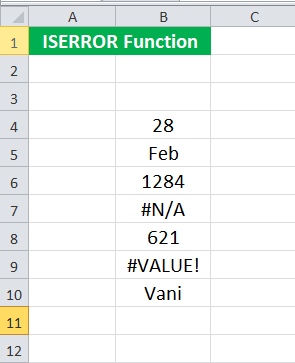
Suppose we want to see if a number gives an error when divided by another number.
We know that a number, when divided by zero, gives an error in ExcelErrors in excel are common and often occur at times of applying formulas. The list of nine most common excel errors are — #DIV/0, #N/A, #NAME?, #NULL!, #NUM!, #REF!, #VALUE!, #####, Circular Reference.read more. Let us check if 21/0 provides an error using the ISERROR in Excel. To do this, we must type the syntax:
= ISERROR ( 21/0 )
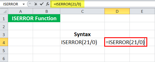
Press the “Enter” key.
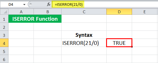
It returns “TRUE.”
We can also refer to cell references in the ISERROR in Excel. Let us now check what will happen when we divide one cell by an empty cell.
When we enter the syntax:
= ISERROR ( A5/B5 )
Given that B5 is an empty cell.
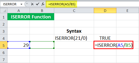
The ISERROR in Excel will return “TRUE.”

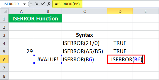
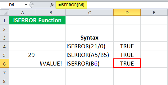
We can also check if any cell contains an error message. Suppose cell B6 has #VALUE! Which is an error in Excel. We may directly input the cell reference in the ISERROR in Excel to check if there is an error message or not as:
= ISERROR ( B6 )
The ISERROR function in Excel will return “TRUE.”
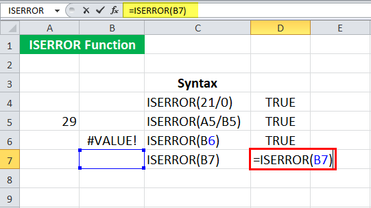
Suppose we refer to an empty cell (B7 in this case) and use the following syntax:
= ISERROR (B7)
Press the “Enter” key.
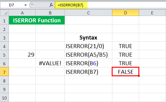
The ISERROR function in Excel may return “FALSE” since the Excel ISERROR function does not check for an empty cell. A blank cell is often considered zero in Excel. So, as we may have noticed above, if we refer to an empty cell in an operation such as division, it will be an error as it is trying to divide it by zero and thus returns “TRUE.”
How to Use the ISERROR Function in Excel?
The ISERROR function in Excel is used to identify cells containing an error. For example, there is often an occurrence of missing values in the data. If a further operation is carried out on such cells, the Excel may get an error. Similarly, if we divide any number by zero, it returns an error. Such errors further intervene if any other operation is carried out on these cells. In such cases, we can first check if there is an error in the operation. If yes, we can choose not to include such cells or modify the operation later.
You can download this ISERROR Function Excel Template here – ISERROR Function Excel Template
ISERROR in Excel Example #1
Suppose we have the actual and forecast values of an experiment. The values are given in cells B4: C15.
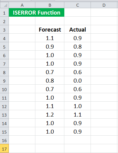
We want to calculate the error rate in this experiment, which is given as (Actual – Forecast) / Actual. However, we also know that some of the actual values are zero, and the error rate for such actual values will give an error. Therefore, we have decided to calculate the error for only those experiments which do not provide an error. To do this, we may use the following syntax for the first set of values:
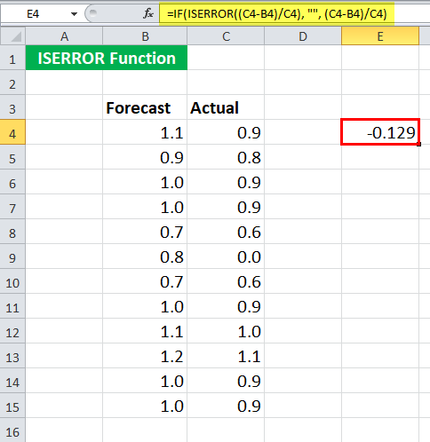
We apply the ISERROR formula in Excel = IF( ISERROR ( (C4-B4) / C4 ), “” , (C4-B4) / C4)
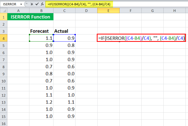
Since the first experimental values do not have any error in calculating the error rate, it will return the error rate.
We will get -0.129
You may now drag it to the rest of the cells.
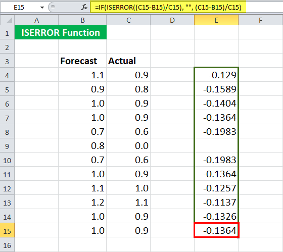
We will realize that the syntax returns no value when the actual value is zero (cell C9).
Now, let us see the syntax in detail.
= IF( ISERROR ( (C4-B4) / C4 ), “” , (C4-B4) / C4 )
- ISERROR ( (C4-B4) / C4 ) will check if the mathematical operation (C4-B4) / C4 gives an error. In this case, it will return “FALSE.”
- If (ISERROR ( (C4-B4) / C4 ) ) returns “TRUE,” the IF function will not return anything.
- If (ISERROR ( (C4-B4) / C4 ) ) returns “FALSE,” the IF function will return (C4-B4) / C4.
ISERROR in Excel Example #2
Suppose we are given some data in B4:B10. Some of the cells contain errors.
We want to check how many cells right from B4: B10 have an error. To do this, we may use the following ISERROR formula in Excel:
= SUMPRODUCT ( — ISERROR ( B4:B10 ) )

And press the “Enter” key.

ISERROR in Excel will return 2 as there are two errors, i.e., #N/A and #VALUE!#VALUE! Error in Excel represents that the reference cell the user has either entered an incorrect formula or used a wrong data type (mostly numerical data). Sometimes, it is difficult to identify the kind of mistake behind this error.read more.
Let us see the syntax in detail:
- ISERROR ( B4:B10 ) will look for errors in B4:B10 and return an array of TRUE or FALSE. Here, it will return {FALSE; FALSE; FALSE; TRUE; FALSE; TRUE; FALSE}
- — ISERROR ( B4:B10 ) will then coerce TRUE/ FALSE to 0 and 1. It will return {0; 0; 0; 1; 0; 1; 0}
- SUMPRODUCT (– ISERROR ( B4:B10 ) ) will then sum {0; 0; 0; 1; 0; 1; 0} and return 2.
ISERROR in Excel Example #3
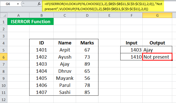
Suppose we have the enrollment ID, name, and marks of students enrolled in the course, given in cells B5:D11.
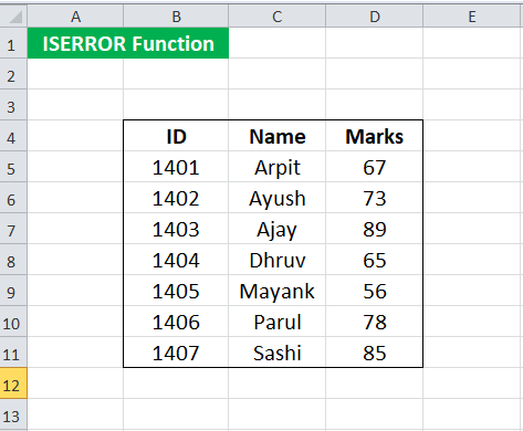
We must search for the student name given its enrollment ID several times. Now, we want to make the search easier by writing a syntax such that:
For any given ID, it should be able to give the corresponding name. Sometimes, the enrollment ID may not be present on the list. In such cases, it should return “Not found.” We can do this by using the ISERROR formula in Excel:
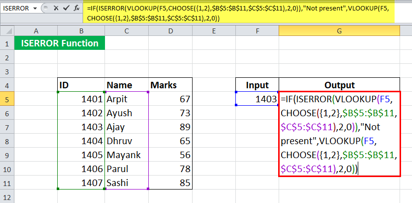
= IF( ISERROR( VLOOKUP( F5, CHOOSE( {1,2}, $B$5:$B$11, $C$5:$C$11 ) , 2, 0) ), “Not present”, VLOOKUP( F5, CHOOSE( {1,2}, $B$5:$B$11, $C$5:$C$11 ), 2, 0) )
Let us look at the ISERROR formula in Excel first:
- CHOOSE( {1,2}, $B$5:$B$11, $C$5:$C$11 ) will make an array and return {1401,”Arpit”; 1402, “Ayush”; 1403, “Ajay”; 1404, “Dhruv”; 1405, “Mayank”; 1406, “Parul”; 1407, “Sashi”}
- VLOOKUP( F5, CHOOSE( {1,2}, $B$5:$B$11, $C$5:$C$11 ) , 2, 0) ) will then look for F5 in the array and return its 2nd
- ISERROR( VLOOKUP( F5, CHOOSE(..) ) will check if there is an error in the function and return TRUE or FALSE.
- IF (ISERROR( VLOOKUP( F5, CHOOSE(..) ), “Not present,” VLOOKUP( F5, CHOOSE() )) will return the corresponding name of the student if present. Else it will return “Not present.”
Use the ISERROR formula in Excel For 1403 in cell F5.
It will return the name “Ajay.”
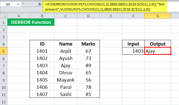
For 1410, the syntax will return “Not present.”
Things to Know about the ISERROR Function in Excel
- The ISERROR function in Excel checks if any given expression returns an error.
- It returns logical values, “TRUE” or “FALSE.”
- It tests for #N/A, #VALUE!, #REF!, #DIV/0!, #NUM!, #NAME?, and #NULL!.
ISERROR Excel Function Video
Recommended Articles
This article is a guide to ISERROR Function in Excel. Here, we discuss the ISERROR formula in Excel and how to use ISERROR in Excel, along with Excel examples and downloadable Excel templates. You may also look at these useful functions in Excel: –
- Fixing VLOOKUP #Name Error
- FORECAST in Excel – Examples
- ISNUMBER in Excel
- INT Function in Excel
- Superscript in Excel
![]()
IFERROR Function in Excel

IFERROR is an Excel Logical Function to Check if a value is an Error. IFERROR used in Excel to handle if the formula is evaluated to an Error. We can handle the Error Cells and Formulas with errors like #VALUE!,#N/A, #REF!, #DIV/0!, #NUM! #NAME? and #NULL!.
In this topic:
- Function
- Syntax
- Parameters
- Usage
- Examples
- IfError Return Values
IFERROR Function
Excel IFError Function helps to return a value if an formula returns an Error. For example, if we enter some formula in Cell, and we assume that there is some chance of getting an Error. In this case we can use IFERROR function to return something else when the formula evaluates an error.
=IFERROR(Actual Formula, Value if the formula returns an Error)
Example:
Let us say you are accepting Total Sales at Range A1 and Units in Range B1. And You wants to calculate the Unit Price at C1. Your formula at C1=A1/B1.
- If the user enters 2000 at Range A1 and 10 at B1, the formula C1 evaluates and returns the unit price as 200.
- What if the user enters 2k at Range A1 and 10 at B1, the formula C1 evaluates to an Error (#VALUE!).
- In this case, we can use IFERROR function to instruct the user to enter valid numbers.
- You can use the formula =IFERROR(A1/B1,”Please Enter Valid Number”) to ask the user to enter valid data.
Syntax
Here is the syntax of the Excel IFERROR Function. It has two required parameters.
IFERROR(value, value_if_error)
Parameters
Excel IFERROR Function takes two parameters. Value is a formula to check for an error. And the second one is the value to be returned if the first argument evaluate an error.
value: Value is a required parameter. This is the Argument which is to be evaluated for an Error. Often, it is a formula or expression.
value_if_error: This is a required parameter. This is the value to return if the formula evaluates to an error. IFERROR returns this value if the first argument evaluates to #N/A, #VALUE!, #REF!, #DIV/0!, #NUM!, #NAME? or #NULL!.
How to use IFERROR in Excel?
IFERROR Functions is used along with other Excel Functions to handle the returning error values. We can combine iferror function while using the reference functions like VLOOKUP, HLOOKUP, XLOOKUP, MATCH, INDEX. We also combine with other conditional aggregate functions like IF, COUNTIF, SUMIF, AVERAGEIF.
Using IFERROR in EXCEL Formula
Let us see how to use IFERROR Function in Excel. We can use the IFERROR function in Excel formula to find if an expression is returning an Error. You can use the IFERROR function to identify the expressions witch may return errors and handle it. IFERROR returns a value you specify if a formula evaluates to an error; otherwise, it returns the result of the formula.
- IFERROR returns a specified value if a formula evaluates to an error; otherwise, it returns the result of the formula
- We can provide a Value , a string or another Expression if the Formula evaluate to an Error
- Often, we use IFERROR with the formulas which may return errors in some (unknown) cases or wrong data inputs. And return some text or value when the formula returns an Error.
Using IFERROR with IF Statement
We can use IFERROR with IF Statement to make conditional and logical checks. Let us see how to use iferror with if statement in Excel formula.
The following example shows how to use IFERROR with IF Statement. User enter some amount at Range B1 and the If formula calculates the Discount Price as Result.
IF Formula =IF(B1>1000,B1*0.1,B1*0.05)
IFERROR + IF Formula =IFERROR(IF(B1>1000,B1*0.1,B1*0.05),”Please Enter Valid Data”)
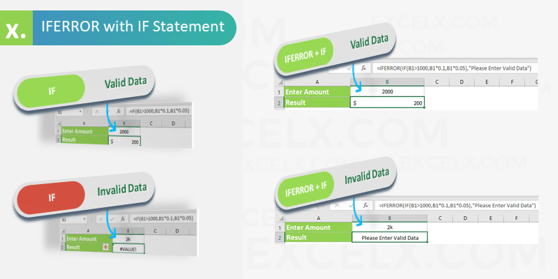
- IF Formula – Valid Data: Calculates and Result the when you enter valid data
- IF Formula – Invalid Data: Calculates and Result the error (#VALUE!) when you enter invalid number.
- IFERROR+IF Formula – Valid Data: Calculates and Result the when you enter valid data
- IFERROR+ IF Formula – Invalid Data: If you enter invalid number, IF Function calculates and Result the error (#VALUE!), IFERROR Evaluates the error and creates the custom message (“Please Enter Valid Data”).
IFERROR Blank
IFERROR Function is used to produce a Blank string if the formula evaluates an Error. Here is the IFERROR Blank Example formula which is common use of IFERROR Function.
Excel If Error Then Blank: If there is any error in the formula then Excel returns Blank using IFERROR. We will take the simple formula to return blank when there is an Error in Excel Formula. To produce a blank string, you can pass the blank string in the second argument of the IFERROR function. Or, you can simply leave the second parameter empty.
Blank String: The following formula will result a BLANK string if the the expression evaluates an Error. Here, we are providing an Blank string character(“”) as the second parameter of the IFERROR Function.
Empty Argument:The following formula will result an Empty Cell if the the expression evaluates an Error. Here, we are not providing the second parameter of the IFERROR Function. We are just closing the function after the comma.
Difference between Providing the Second Argument and Leaving Empty: Function creates a Blank String Character(“”), overwrites the default cell format when you pass the second character. If you leave empty, this will creates cell with default format (as if you entered nothing in the cell).
IFERROR VLOOKUP
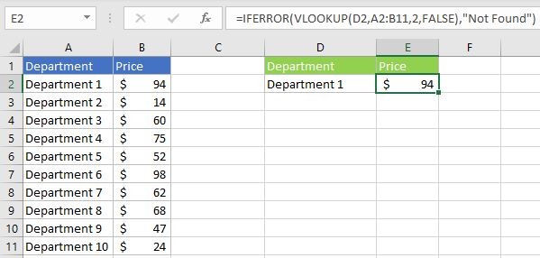
IFERROR is used with the combination of VLOOKUP function. VLOOKUP function returns an error value (#NA) if it is not found the lookup value in the lookup table array range. We can suppress these errors using IFERROR function with VLOOKUP. Otherwise, we can perform another operation if Vlookup returns an Error.
Let us see an example to understand how to use IFERROR and VLOOKUP together. VLOOKUP tries to find the lookup value (D2) in the lookup table array (A2:B11) and returns the corresponding value in column 2. If VLOOKUP not find the value in the given range, IFERROR Returns a string (“Not found”)
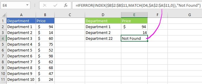
IFERROR INDEX MATCH
We use INDEX and MATCH Functions to create Advanced VLOOKUP Formula. We can use IFERROR with the combination of INDEX and MATCH functions (as used in the VLOOKUP function). INDEX and MATH Lookup functions returns an error value (#NA) if the lookup value is not found the lookup range. We can use IFERROR function to produce the alternative string.
Here is a simple example to show you how to use IFERROR function along with INDEX and MATCH reference functions. MATCH function returns the match position of the lookup value (D4) in the lookup range ($A$2:$A$11). And the INDEX function returns the value from the reference ($B$2:$B$11) from the row number returned by MATCH function. Match returns #NA error if the given lookup value is not found in the lookup range. We can use IFERROR to Returns a new string (“Not found”)
IF And IFERROR Combined
We can Combine IF and IFERROR Functions in Excel to create issue free Formulas. We can check some expression using IF Function. And trap the result using IFERROR function.
This formula will checks an expression using IF and returns the defined value. If it returns an error, error message will be displayed in the Cell.
IF IFERROR and VLOOKUP
We can also Combine IF, IFERROR Functions with VLOOKUP in Excel to create advanced Formulas. VLOOKUP fetch a value from table range. And the IFERROR Evaluates the VLOOKUP output. Finally, IF functions makes the decision to display the value based on the result.
Here is real-time example to understand how to use IFERROR and VLOOKUP together in the same formula.
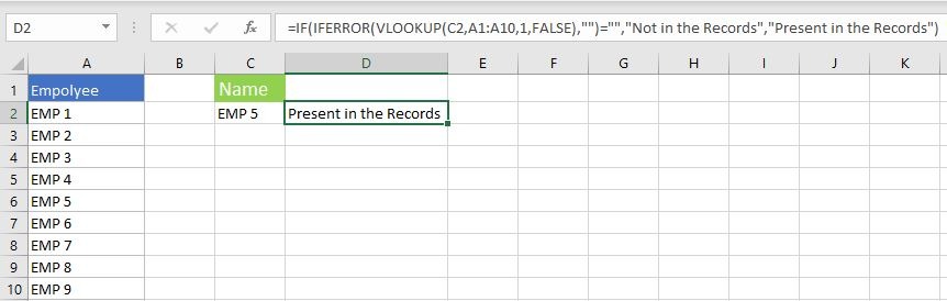
- In this formula, VLOOKUP will check for an EMP Record
- IFERROR returns blank if no record is found
- IF statement will display the message based on the result
Nested IFERROR
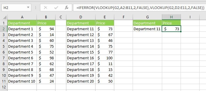
Nested IFERROR formula is helpful to fetch the values from multiple references. Following is the example of Nested IFERROR with VLOOKUP function to check for a value in two different ranges and return the corresponding column value. If the lookup values is not found in both the ranges, return custom value or a text.
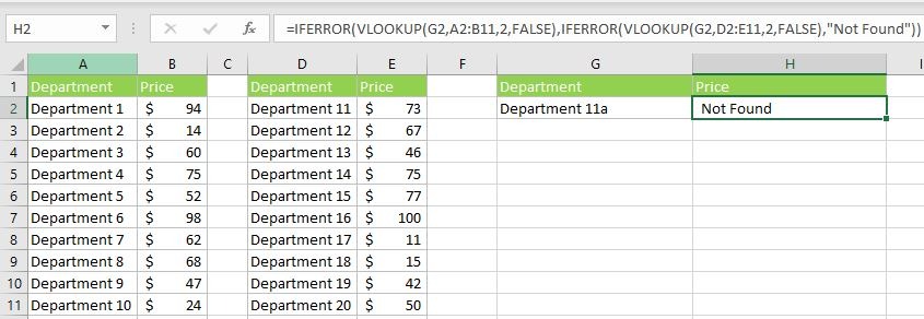
- VLOOKUP(G2,A2:B11,2,FALSE) : checks for a value G2 in the first range A2:B11
- =IFERROR(VLOOKUP(G2,A2:B11,2,FALSE), : This will checks the return value and out put the corresponding value. If it is not found in the given range (A2:B11). IFERROR process the second part of the formula (i.e; IFERROR(VLOOKUP(G2,D2:E11,2,FALSE),”Not Found”))
- VLOOKUP(G2,D2:E11,2,FALSE):checks for a value G2 in the first range D2:E11
- IFERROR(VLOOKUP(G2,D2:E11,2,FALSE),”Not Found”) : This will checks the return value of 2nd VLOOKUP and out put the corresponding value. If it is not found in the given range (D2:E11). IFERROR process the second argument of the function and returns the string “Not Found”
Nested IFERROR and IF
We can add the IF Function with Nested IFERROR function to return the value based on the result. We can use the above formula and display the value in the cell using IF Function.
Here, we have added Function to display a message as “Need to Add”,”Exist in the Table” based on the Nested IfError and If function.
Excel IFERROR Else
We can make use of this formula to check if an expression evaluates an Error then display some value. Else display another Value.
Comparing IFERROR with Other Function
We have many functions to handle the Errors in Excel. Let us see the different Error trapping Functions in Excel and how they are different from IFERROR function.
ISERROR vs IFERROR
ISERROR Function is useful to check if an expression evaluates to an error or not. IFERROR Helps to replace that error with some value.
IF ISERROR vs IFERROR
If ISERROR combination is useful when you wants to check an expression and execute Expression One when it is True and Expression Two when it is False.
IFNA vs IFERROR
IFNA Function is used when you wants to replace only if an expression returns #NA Error. Where as IFERROR is helps to tackle with any type of errors listed above.
ISNA vs IFERROR
ISNA Function is used to check if an expression is Returning a #NA type Error. IFERROR is used to replace an error if the expression evaluates to any error listed above.
IF and IFERROR
IF Function is used to check a condition and executes the first expression when it is True and the second expression when it is False. But IFERROR is used when you want to replace an error only if the expression evaluates to any error listed above.
IFERROR vs IFNA for VLOOKUP
VlookUp returns #NA type error if the lookup value is not found in the table array. You can use IFNA function to deal with this situation. But, in some cases the VlookUp return other type of Errors like #Name (based on the input expressions). You can use IfError to deal with any type of Errors as mention above.
How Does IFERROR Work
IFERROR Works as error handling formula in Excel. Following is the process flow chart of IFERROR Function with clear instructions.
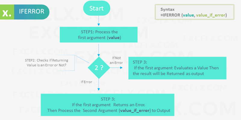
- It required two arguments to process the function
- It will process the first argument and validate the evaluated value
- If the first argument returns the value which is not an error (#VALUE!,#N/A, #REF!, #DIV/0!, #NUM! #NAME? and #NULL!.), then it returns the result output of the first argument
- If the first argument returns an error, then it will process the second argument of the IFERROR function and returns the output
Here are the simple examples to understand how does IFERROR function Works. The first example returns the actual value, and the second example returns the IFERROR function value.
Example 1: We have provided the First argument as 25+75, tried to add number and number. It returns the values as 100. So, the IFERROR function Returns the first argument.
Formula
Output:100
Example 2: We have provided the First argument as 25+”Some Text”, tried to add number and string. It returns an Error. So, the IFERROR function Returns the second argument.
Formula
Output:”You can not add a number and Text”
IFERROR Examples
1. Display Message to User
Here is a simple example to explain the IFERROR Function. The following Formula check the first expression and returns the given string as it evaluates an Error.
Formula:
=IFERROR(5/0,”Please Enter Valid Number”)Returns: Please Enter Valid Number
We can see the first argument of the formula (5/0) evaluates #DIV/0! Error. And IFERROR function trap this error and returns the second argument.
2. IFERROR Then Return 0
Let us say we are performing a calculation based on the result. If there is any Error in the Formula, we want the Excel to return Zero. In this case we can use iferror and simply return 0 if the formula evaluates to an Error.
Formula:
Returns: 0 (if the formula evaluates to an error)
3. IFERROR, Make the Cell Blank
Excel sheet do not look good if there are many Error Cells . We can use the IFERROR formula to return a blank if the formula returns errors.
Formula:
Returns: “” (if the formula evaluates to an error)
4. Check if a value found in List of values
IFEEROR helps to determine if an item found in the list of items, range or Array. The following Example checks if value find in a range of values.
5. If Error then Evaluate another Formula
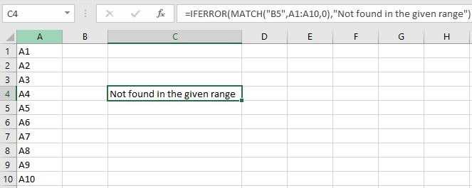
The following formula checks for a value in Range A1:A10. If it is not found in the A1:B10, IFERROR helps to check in another Range(D1:E10). Here is a simple example on IFERROR to return a value from one of the Ranges.
IFERROR Return Values
Excel IFERROR can be used to return values based on our requirement. We can return a string, a number, or evaluate a formula. Let us see the most widely returning Values of IFERROR Function.
| Return Value | Formula | Description |
|---|---|---|
| BLANK | =IFERROR(IF(B2>1000,B2*0.1,B2*0.05),””) | Return BLANK
IfError Then BLANK |
| NULL | =IFERROR(IF(B3>1000,B3*0.1,B3*0.05),””) | Return NULL
IfError Then NULL |
| EMPTY | =IFERROR(IF(B4>1000,B4*0.1,B4*0.05),””) | Return EMPTY
IfError Then EMPTY |
| Empty Cell | =IFERROR(IF(B5>1000,B5*0.1,B5*0.05),””) | Return Empty Cell
IfError Then Empty Cell |
| Nothing | =IFERROR(IF(B6>1000,B6*0.1,B6*0.05),””) | Return Nothing
IfError Then Nothing |
| No Value | =IFERROR(IF(B7>1000,B7*0.1,B7*0.05),”No Value Found”) | Return No Value
IfError Then No Value |
| Original Value | =IFERROR(IF(B8>1000,B8*0.1,B8*0.05),B8) | Return Original Value
IfError Then Original Value |
| TRUE | =IFERROR(IF(B9>1000,B9*0.1,B9*0.05),TRUE) | Return TRUE
IfError Then TRUE |
| FALSE | =IFERROR(IF(B10>1000,B10*0.1,B10*0.05),FALSE) | Return FALSE
IfError Then FALSE |
| 0 | =IFERROR(IF(B11>1000,B11*0.1,B11*0.05),0) | Return 0
IfError Then 0 |
| Blank Instead of 0 | =IFERROR(IF(B12>1000,B12*0.1,B12*0.05),””) | Return Blank Instead of 0
IfError Then Blank Instead of 0 |
| Blank Text Instead of 0 | =IFERROR(IF(B13>1000,B13*0.1,B13*0.05),”BLANK”) | Return Blank Text Instead of 0
IfError Then Blank Text Instead of 0 |
| Null Text | =IFERROR(IF(B14>1000,B14*0.1,B14*0.05),”NULL”) | Return Null Text
IfError Then Null Text |
| EMPTY Text | =IFERROR(IF(B15>1000,B15*0.1,B15*0.05),”EMPTY”) | Return EMPTY Text
IfError Then EMPTY Text |
| ERROR Text | =IFERROR(IF(B16>1000,B16*0.1,B16*0.05),”ERROR”) | Return ERROR Text
IfError Then ERROR Text |
| N/A Text | =IFERROR(IF(B17>1000,B17*0.1,B17*0.05),”N/A”) | Return N/A Text
IfError Then N/A Text |
| Hyphen (-) | =IFERROR(IF(B18>1000,B18*0.1,B18*0.05),”-“) | Return Hyphen (-)
IfError Then Hyphen (-) |
| Question Mark (?) | =IFERROR(IF(B19>1000,B19*0.1,B19*0.05),”?”) | Return Question Mark (?)
IfError Then Question Mark (?) |
| Zero | =IFERROR(IF(B20>1000,B20*0.1,B20*0.05),”Zero”) | Return Zero
IfError Then Zero |
| Text | =IFERROR(IF(B21>1000,B21*0.1,B21*0.05),”Your Text”) | Return Text
IfError Then Text |
| Error | =IFERROR(IF(B22>1000,B22*0.1,B22*0.05),”Error”) | Return Error
IfError Then Error |
| NA | =IFERROR(IF(B23>1000,B23*0.1,B23*0.05),NA()) | Return NA
IfError Then NA |
| Space | =IFERROR(IF(B24>1000,B24*0.1,B24*0.05),” “) | Return Space
IfError Then Space |
| Value | =IFERROR(IF(B25>1000,B25*0.1,B25*0.05),”1000″) | Return Value
IfError Then Value |
| Cell Value | =IFERROR(IF(B26>1000,B26*0.1,B26*0.05),B26) | Return Cell Value
IfError Then Cell Value |
| Another Cell | =IFERROR(IF(B27>1000,B27*0.1,B27*0.05),A27) | Return Another Cell
IfError Then Another Cell |
| Number | =IFERROR(IF(B28>1000,B28*0.1,B28*0.05),”25″) | Return Number
IfError Then Number |
| Row | =IFERROR(IF(B29>1000,B29*0.1,B29*0.05),ROW()) | Return Row
IfError Then Row |
| Column | =IFERROR(IF(B30>1000,B30*0.1,B30*0.05),COLUMN()) | Return Column
IfError Then Column |
| Date | =IFERROR(IF(B31>1000,B31*0.1,B31*0.05),TODAY()) | Return Date
IfError Then Date |
| Error | =IFERROR(IF(B32>1000,B32*0.1,B32*0.05),CELL(“type”)) | Return Error
IfError Then Error |
Return 0:
We can use IFERROR to return 0 if the formula evaluates an Error. This is very helpful while processing the numerical data. If you have the formulas witch are resulting an Error while calculation, it will effect the all other calculations. If you return 0 using IFERROR, you can avoid those issues with your spreadsheet.
Formula:
Return Blank:
If you are dealing with string data, you can return blank instead of 0. It makes your sheet more cleaner and issue free. Following is the formula to Return Blank if there are any errors in Formula.
Formula:
Return Null:
You can make use of IFERROR and return Null string to avoid conflicts with other formula. Here is
Best Practices
Please remember the following best practices to be followed while using IFERROR in Excel Formula.
- IFERROR is very important and useful formula to create an issue free spreadsheet worksheet. Use this formula when there is a chance of evaluation error.
- Try to use smaller portion of the formula, instead of the entire formula.
- Do not leave the arguments empty. IFERROR treats the empty arguments as an Empty String (“”).
- Try to Avoid using IF + ISERROR , instead use IFERROR Function
- Use ISNA function to check if the expression evaluates only #NA Error, otherwise use IFERROR to catch all Errors
- ISERR function to check if the expression evaluates errors except #NA Error
Share This Story, Choose Your Platform!
© Copyright 2012 – 2020 | Excelx.com | All Rights Reserved
Page load link
When you work with data and formulas in Excel, you’re bound to encounter errors.
To handle errors, Excel has provided a useful function – the IFERROR function.
Before we get into the mechanics of using the IFERROR function in Excel, let’s first go through the different kinds of errors you can encounter when working with formulas.
Types of Errors in Excel
Knowing the errors in Excel will better equip you to identify the possible reason and the best way to handle these.
Below are the types of errors you might find in Excel.
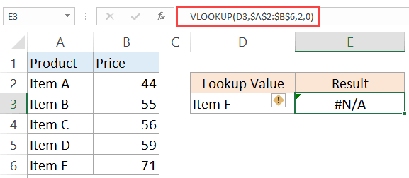
#N/A Error
This is called the ‘Value Not Available’ error.
You will see this when you use a lookup formula and it can’t find the value (hence Not Available).
Below is an example where I use the VLOOKUP formula to find the price of an item, but it returns an error when it can’t find that item in the table array.
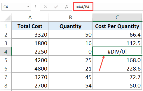
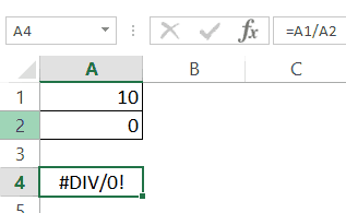
#DIV/0! Error
You’re likely to see this error when a number is divided by 0.
This is called the division error. In the below example, it gives a #DIV/0! error as the quantity value (the divisor in the formula) is 0.
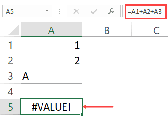
#VALUE! Error
The value error occurs when you use an incorrect data type in a formula.
For example, in the below example, when I try to add cells that have numbers and character A, it gives the value error.
This happens as you can only add numeric values, but instead, I tried adding a number with a text character.
#REF! Error
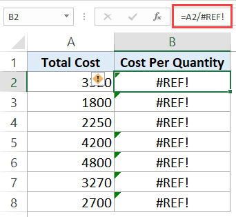
This is called the reference error and you will see this when the reference in the formula is no longer valid. This could be the case when the formula refers to a cell reference and that cell reference does not exist (happens when you delete a row/column or worksheet that was referred to in the formula).
In the below example, while the original formula was =A2/B2, when I deleted Column B, all the references to it became #REF! and it also gave the #REF! error as the result of the formula.
#NAME ERROR
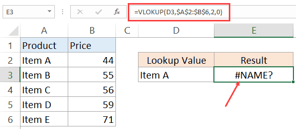
This error is likely to a result of a misspelled function.
For example, if instead of VLOOKUP, you by mistake use VLOKUP, it will give a name error.
#NUM ERROR
Num error can occur if you try and calculate a very large value in Excel. For example, =187^549 will return a number error.
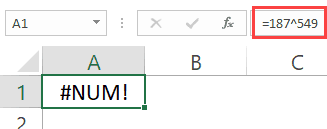
Another situation where you can get the NUM error is when you give a non-valid number argument to a formula. For example, if you’re calculating the Square Root if a number and you give a negative number as the argument, it will return a number error.
For example, in the case of Square Root function, if you give a negative number as the argument, it will return a number error (as shown below).
While I have shown only a couple of examples here, there can be many other reasons that can lead to errors in Excel. When you get errors in Excel, you can’t just leave it there. If the data is further used in calculations, you need to make sure the errors are handled the right way.
Excel IFERROR function is a great way to handle all types of errors in Excel.
Excel IFERROR Function – An Overview
Using the IFERROR function, you can specify what you want the formula to return instead of the error. If the formula does not return an error, then its own result is returned.
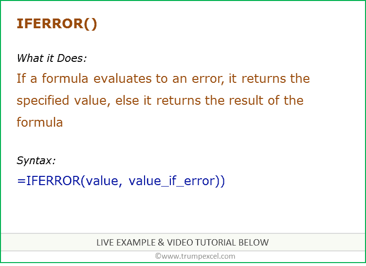
IFERROR Function Syntax
=IFERROR(value, value_if_error)
Input Arguments
- value – this is the argument that is checked for the error. In most cases, it is either a formula or a cell reference.
- value_if_error – this is the value that is returned if there is an error. The following error types evaluated: #N/A, #REF!, #DIV/0!, #VALUE!, #NUM!, #NAME?, and #NULL!.
Additional Notes:
- If you use “” as the value_if_error argument, the cell displays nothing in case of an error.
- If the value or value_if_error argument refers to an empty cell, it is treated as an empty string value by the Excel IFERROR function.
- If the value argument is an array formula, IFERROR will return an array of results for each item in the range specified in value.
Excel IFERROR Function – Examples
Here are three examples of using IFERROR function in Excel.
Example 1 – Return Blank Cell Instead of Error
If you have functions that may return an error, you can wrap it within the IFERROR function and specify blank as the value to return in case of an error.
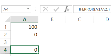
In the example shown below, the result in D4 is the #DIV/0! error as the divisor is 0.
In this case, you can use the following formula to return blank instead of the ugly DIV error.
=IFERROR(A1/A2,””)
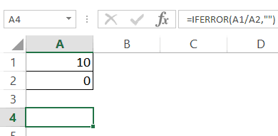
This IFERROR function would check whether the calculation leads to an error. If it does, it simply returns a blank as specified in the formula.
Here, you can also specify any other string or formula to display instead of the blank.
For example, the below formula would return the text “Error”, instead of the blank cell.
=IFERROR(A1/A2,”Error”)

Note: If you are using Excel 2003 or a prior version, you will not find the IFERROR function in it. In such cases, you need to use the combination of IF function and ISERROR function.
Example 2 – Return ‘Not Found’ when VLOOKUP Can’t Find a Value
When you use the Excel VLOOKUP Function, and it can’t find the lookup value in the specified range, it would return the #N/A error.
For example, below is a data set of student names and their marks. I have used the VLOOKUP function to fetch the marks of three students (in D2, D3, and D4).
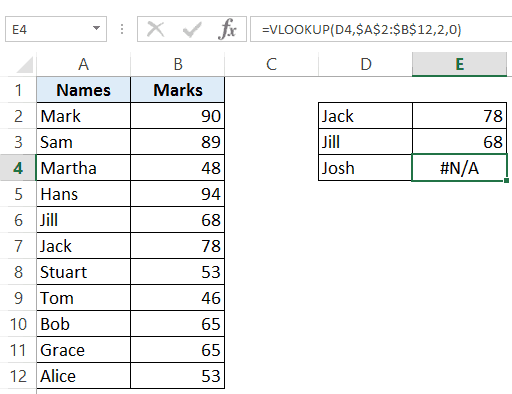
While the VLOOKUP formula in the above example finds the names of first two students, it can’t find Josh’s name on the list and hence it returns the #N/A error.
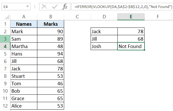
Here, we can use the IFERROR function to return a blank or some meaningful text instead of the error.
Below is the formula that will return ‘Not Found’ instead of the error.
=IFERROR(VLOOKUP(D2,$A$2:$B$12,2,0),”Not Found”)
Note that you can also use IFNA instead of IFERROR with VLOOKUP. While IFERROR would treat all kinds of error values, IFNA would only work on the #N/A errors and wouldn’t work with other errors.
Example 3 – Return 0 in case of an Error
If you don’t specify the value to return by IFERROR in the case of an error, it would automatically return 0.
For example, if I divide 100 with 0 as shown below, it would return an error.
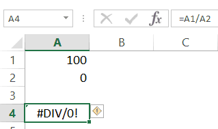
However, if I use the below IFERROR function, it would return a 0 instead. Note that you still need to use a comma after the first argument.
Example 4 – Using Nested IFERROR with VLOOKUP
Sometimes when using VLOOKUP, you may have to look through the fragmented table of arrays. For example, suppose you have the sales transaction records in 2 separate worksheets and you want to look-up an item number and see it’s value.
Doing this requires using nested IFERROR with VLOOKUP.
Suppose you have a dataset as shown below:
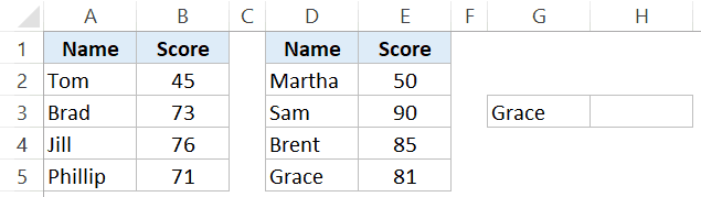
In this case, to find the score for Grace, you need to use the below nested IFERROR formula:
=IFERROR(VLOOKUP(G3,$A$2:$B$5,2,0),IFERROR(VLOOKUP(G3,$D$2:$E$5,2,0),"Not Found"))
This kind of formula nesting ensure that you get the value from either of the table and any error returned is handled.
Note that in case the tables are on the same worksheet, however, in a real-life example, it likely to be on different worksheets.
Excel IFERROR Function – VIDEO
Related Excel Functions:
- Excel AND Function.
- Excel OR Function.
- Excel NOT Function.
- Excel IF Function.
- Excel IFS Function.
- Excel FALSE Function.
- Excel TRUE Function.
You May Also Like the Following Excel Tutorials:
- Use IFERROR with VLOOKUP to Get Rid of #N/A Errors.
- Identify Errors Using Excel Formula Debugging.
Функция IFERROR (ЕСЛИОШИБКА) в Excel лучше всего подходит для обработки случаев, когда формулы возвращают ошибку. Используя эту функцию, вы можете указать, какое значение функция должна возвращать вместо ошибки. Если функция в ячейке не возвращает ошибку, то возвращается её собственный результат.
Содержание
- Видеоурок
- Что возвращает функция
- Синтаксис
- Аргументы функции
- Дополнительная информация
- Примеры использования функции IFERROR (ЕСЛИОШИБКА) в Excel
- Пример 1. Заменяем ошибки в ячейке на пустые значения
- Пример 2. Заменяем значения без данных при использовании функции VLOOKUP (ВПР) на “Не найдено”
- Пример 3. Возвращаем значение “0” вместо ошибок формулы
Видеоурок
Что возвращает функция
Указанное вами значение, в случае если в ячейке есть ошибка.
Синтаксис
=IFERROR(value, value_if_error) — английская версия
=ЕСЛИОШИБКА(значение;значение_если_ошибка) — русская версия
Аргументы функции
- value (значение) — это аргумент, который проверяет, есть ли в ячейке ошибка. Обычно, ошибкой может быть результат какого либо вычисления;
- value_if_error (значение_если_ошибка) — это аргумент, который заменяет ошибку в ячейке (в случае её наличия) на указанное вами значение. Ошибки могут выглядеть так: #N/A, #REF!, #DIV/0!, #VALUE!, #NUM!, #NAME?, #NULL! (английская версия Excel) или #ЗНАЧ!, #ДЕЛ/0, #ИМЯ?, #Н/Д, #ССЫЛКА!, #ЧИСЛО!, #ПУСТО! (русская версия Excel).
Дополнительная информация
- Если вы используете кавычки («») в качестве аргумента value_if_error (значение_если_ошибка), ячейка ничего не отображает в случае ошибки.
- Если аргумент value (значение) или value_if_error (значение_если_ошибка) ссылается на пустую ячейку, она рассматривается как пустая.
Примеры использования функции IFERROR (ЕСЛИОШИБКА) в Excel
Пример 1. Заменяем ошибки в ячейке на пустые значения
Если вы используете функции, которые могут возвращать ошибку, вы можете заключить ее в функцию и указать пустое значение, возвращаемое в случае ошибки.
В примере, показанном ниже, результатом ячейки D4 является # DIV/0!.
Для того, чтобы убрать информацию об ошибке в ячейке используйте эту формулу:
=IFERROR(A1/A2,””) — английская версия
=ЕСЛИОШИБКА(A1/A2;»») — русская версия

В данном случае функция проверит, выдает ли формула в ячейке ошибку, и, при её наличии, выдаст пустой результат.
В качестве результата формулы, исправляющей ошибки, вы можете указать любой текст или значение, например, с помощью следующей формулы:
=IFERROR(A1/A2,”Error”) — английская версия
=ЕСЛИОШИБКА(A1/A2;»») — русская версия
Если вы пользуетесь версией Excel 2003 или ниже, вы не найдете функцию IFERROR (ЕСЛИОШИБКА). Вместо нее вы можете использовать обычную функцию IF или ISERROR.
Пример 2. Заменяем значения без данных при использовании функции VLOOKUP (ВПР) на “Не найдено”
Когда мы используем функцию VLOOKUP (ВПР), часто сталкиваемся с тем, что при отсутствии данных по каким либо значениям, формула выдает ошибку “#N/A”.
На примере ниже, мы хотим с помощью функции VLOOKUP (ВПР) для выбранных студентов подставить данные из результатов экзамена.
На примере выше, в списке студентов с результатами экзамена нет данных по имени Иван, в результате, при использовании функции VLOOKUP (ВПР), формула нам выдает ошибку.
Как раз в этом случае мы можем воспользоваться функцией IFERROR (ЕСЛИОШИБКА), для того, чтобы результат вычислений выглядел корректно, без ошибок. Добиться этого мы можем с помощью формулы:
=IFERROR(VLOOKUP(D2,$A$2:$B$12,2,0),”Не найдено”) — английская версия
=ЕСЛИОШИБКА(ВПР(D2;$A$2:$B$12;2;0);»Не найдено») — русская версия
Пример 3. Возвращаем значение “0” вместо ошибок формулы
Если у вас нет конкретного значения, которое вы бы хотели использовать для замены ошибок — оставляйте аргумент функции value_if_error (значение_если_ошибка) пустым, как показано на примере ниже и в случае наличия ошибки, функция будет выдавать “0”:
Return value
The value you specify for error conditions.
Usage notes
The IFERROR function is used to catch errors and return a more friendly result or message when an error is detected. When a formula returns a normal result, the IFERROR function returns that result. When a formula returns an error, IFERROR returns an alternative result. IFERROR is an elegant way to trap and manage errors. The IFERROR function is a modern alternative to the ISERROR function.
Use the IFERROR function to trap and handle errors produced by other formulas or functions. IFERROR checks for the following errors: #N/A, #VALUE!, #REF!, #DIV/0!, #NUM!, #NAME?, or #NULL!.
Example #1
In the example shown, the formula in E5 copied down is:
=IFERROR(C5/D5,0)
This formula catches the #DIV/0! error that occurs when Qty is empty or zero, and replaces it with zero.
Example #2
For example, if A1 contains 10, B1 is blank, and C1 contains the formula =A1/B1, the following formula will catch the #DIV/0! error that results from dividing A1 by B1:
=IFERROR (A1/B1,"Please enter a value in B1")
As long as B1 is empty, C1 will display the message «Please enter a value in B1» if B1 is blank or zero. When a number is entered in B1, the formula will return the result of A1/B1.
Example #3
You can also use the IFERROR function to catch the #N/A error thrown by VLOOKUP when a lookup value isn’t found. The syntax looks like this:
=IFERROR(VLOOKUP(value,data,column,0),"Not found")
In this example, when VLOOKUP returns a result, IFERROR functions that result. If VLOOKUP returns #N/A error because a lookup value isn’t found, IFERROR returns «Not Found».
IFERROR or IFNA?
The IFERROR function is a useful function, but it is a blunt instrument since it will trap many kinds of errors. For example, if there’s a typo in a formula, Excel may return the #NAME? error, but IFERROR will suppress the error and return the alternative result. This can obscure an important problem. In many cases, it makes more sense to use the IFNA function, which only traps the #N/A error.
Other error functions
Excel provides a number of error-related functions, each with a different behavior:
- The ISERR function returns TRUE for any error type except the #N/A error.
- The ISERROR function returns TRUE for any error.
- The ISNA function returns TRUE for #N/A errors only.
- The ERROR.TYPE function returns the numeric code for a given error.
- The IFERROR function traps errors and provides an alternative result.
- The IFNA function traps #N/A errors and provides an alternative result.
Notes
- If value is empty, it is evaluated as an empty string («») and not an error.
- If value_if_error is supplied as an empty string («»), no message is displayed when an error is detected.
- In Excel 2013+, you can use the IFNA function to trap and handle #N/A errors specifically.
|
se_arts  Пользователь Сообщений: 20 |
#1 13.03.2018 10:34:11 Подскажите, пожалуйста, как правильно задается условие «если ошибка»
Прикрепленные файлы
|
||
|
Hugo Пользователь Сообщений: 23134 |
#2 13.03.2018 10:39:41
|
||
|
se_arts Пользователь Сообщений: 20 |
#3 13.03.2018 11:48:34
Выдает ошибку: Изменено: se_arts — 13.03.2018 22:48:11 |
|||
|
ZVI  Пользователь Сообщений: 4328 |
#4 13.03.2018 12:36:14
|
||
|
Дмитрий Щербаков  Пользователь Сообщений: 13997 Профессиональная разработка приложений для MS Office |
#5 13.03.2018 12:45:42
В любом случае надо разбивать на два отдельных условия:
Но если надо проверять на ЛЮБЫЕ ошибки — то лучше воспользоваться вариантом ZVI
Даже самый простой вопрос можно превратить в огромную проблему. Достаточно не уметь формулировать вопросы… |
||||||
|
se_arts Пользователь Сообщений: 20 |
#6 13.03.2018 14:24:57 Дмитрий, все равно выдает ошибку «13»
Пробую разные варианты — выдает одну и туже ошибку «13» — может я синтаксис неверно пишу? Изменено: se_arts — 13.03.2018 22:47:07 |
||
|
sokol92  Пользователь Сообщений: 4429 |
У Вас ошибка выдается в строке (при i=16), следующей за заголовком цикла, которую Вы как раз не меняете во всех тестах. Смело нажимайте на Debug и убедитесь самостоятельно. Изменено: sokol92 — 13.03.2018 15:32:43 |
|
Hugo Пользователь Сообщений: 23134 |
#8 13.03.2018 22:43:51 Посмотрел наконец файл — точно xlErrValue нужно:
Или можно конечно искать просто «Error 2015» |
||