Excel for Microsoft 365 Excel for Microsoft 365 for Mac Excel for the web Excel 2021 Excel 2021 for Mac Excel 2019 Excel 2019 for Mac Excel 2016 Excel for iPad Excel Web App Excel for iPhone Excel for Android tablets Excel for Android phones More…Less
#SPILL errors are returned when a formula returns multiple results, and Excel cannot return the results to the grid. For more details on these error types, see the following help topics:
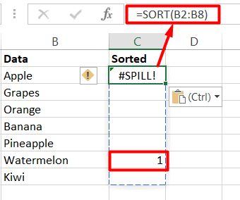
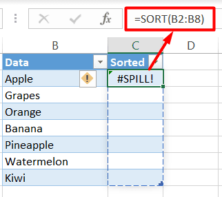
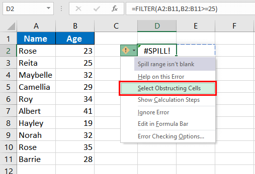
This error occurs when the spill range for a spilled array formula isn’t blank.
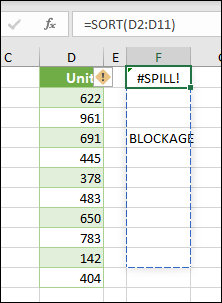
When the formula is selected, a dashed border will indicate the intended spill range.
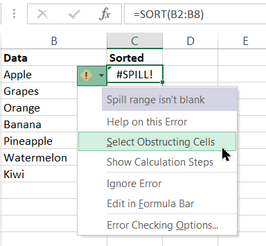
You can select the Error floatie, and choose the Select Obstructing Cells option to immediately go the obstructing cell(s). You can then clear the error by either deleting, or moving the obstructing cell’s entry. As soon as the obstruction is cleared, the array formula will spill as intended.
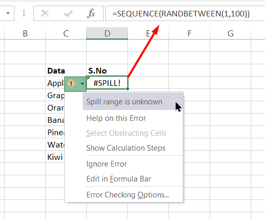
Excel was unable to determine the size of the spilled array because it’s volatile, and resizes between calculation passes. For instance, the following formula will trigger this #SPILL! error:
=SEQUENCE(RANDBETWEEN(1,1000))
Dynamic array resizes may trigger additional calculation passes to ensure the spreadsheet is fully calculated. If the size of the array continues to change during these additional passes and does not stabilize, Excel will resolve the dynamic array as #SPILL!.
This error value is generally associated with the use of RAND, RANDARRAY, and RANDBETWEEN functions. Other volatile functions such as OFFSET, INDIRECT, and TODAY do not return different values on every calculation pass.
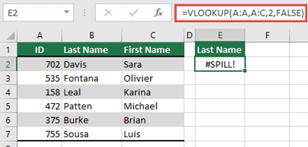
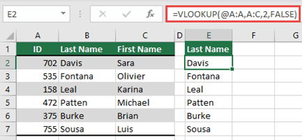
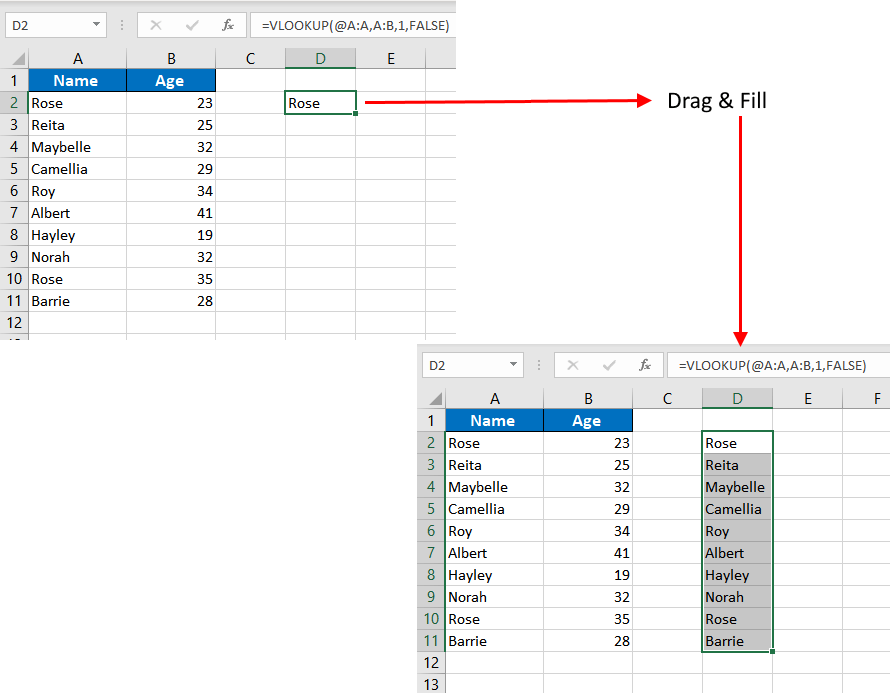
For example, when placed in cell E2 as in the example below, the formula =VLOOKUP(A:A,A:C,2,FALSE) would previously only lookup the ID in cell A2 . However, in dynamic array Excel, the formula will cause a #SPILL! error because Excel will lookup the entire column, return 1,048,576 results, and hit the end of the Excel grid.
There are 3 simple ways to resolve this issue:
|
# |
Approach |
Formula |
|---|---|---|
|
1 |
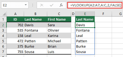
Reference just the lookup values you are interested in. This style of formula will return a dynamic array, but does not work with Excel tables.
|
=VLOOKUP(A2:A7,A:C,2,FALSE) |
|
2 |
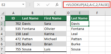
Reference just the value on the same row, and then copy the formula down. This traditional formula style works in tables, but will not return a dynamic array.
|
=VLOOKUP(A2,A:C,2,FALSE) |
|
3 |
Request that Excel perform implicit intersection using the @ operator, and then copy the formula down. This style of formula works in tables, but will not return a dynamic array.
|
=VLOOKUP(@A:A,A:C,2,FALSE) |
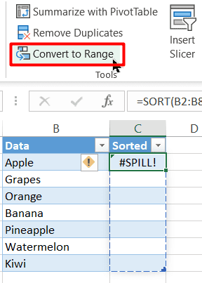
Spilled array formulas aren’t supported in Excel tables. Try moving your formula out of the table, or converting the table to a range (click Table Design > Tools > Convert to range).
The spilled array formula you’re attempting to enter has caused Excel to run out of memory. Please try referencing a smaller array or range.
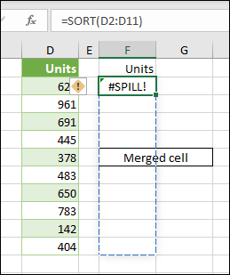
Spilled array formulas cannot spill into merged cells. Please un-merge the cells in question, or move the formula to another range that doesn’t intersect with merged cells.
When the formula is selected, a dashed border will indicate the intended spill range.
You can select the Error floatie, and choose the Select Obstructing Cells option to immediately go the obstructing cell(s). As soon as the merged cells are cleared, the array formula will spill as intended.
Excel doesn’t recognize, or can’t reconcile the cause of this error. Please make sure your formula contains all the required arguments for your scenario.
Need more help?

See also
You can always ask an expert in the Excel Tech Community or get support in the Answers community.
FILTER function
RANDARRAY function
SEQUENCE function
SORT function
SORTBY function
UNIQUE function
Dynamic arrays and spilled array behavior
Implicit intersection operator: @
Need more help?
Пользователи просили нас ответить на два наиболее часто задаваемых вопроса: что такое ошибка Excel Spill и как от нее избавиться. Бывают случаи, когда объяснение этому простое, но бывают и ситуации, когда оно не столь ясно.
Поскольку в Excel была добавлена функция динамических массивов, формулы, которые возвращают несколько значений, теперь переносят эти значения прямо на рабочий лист, где они были первоначально рассчитаны.
Область, содержащая значения, называется диапазоном разлива и представляет собой прямоугольник. При обновлении статистики диапазон разливов будет скорректирован с учетом любого необходимого расширения или сокращения. Вы можете увидеть, как добавляются новые значения, или вы можете видеть, что уже существующие значения удаляются.
Что означает ошибка разлива в Excel?
Ошибка Spill возникает чаще всего, когда диапазон разлива на рабочем листе блокируется другим элементом рабочего листа. Это следует ожидать при случае.
Например, вы ввели формулу и ожидаете, что она прольется. Но на листе уже есть данные, которые его блокируют.

Источник: поддержка Майкрософт
Проблема может быть легко решена путем удаления любых данных, которые могут блокировать диапазон разлива. Если щелкнуть указание ошибки Spill, вы получите более подробную информацию о проблеме, вызвавшей проблему.
Важно понимать, что поведение разливов является как инстинктивным, так и естественным. Любая формула, даже не включающая никаких функций, способна выдать результаты в Dynamic Excel (Excel 365).
Несмотря на то, что существуют методы, предотвращающие получение формулой многочисленных результатов, сброс нельзя отключить с помощью глобальной опции.
Точно так же в Excel нет параметра, позволяющего пользователям отключать ошибки Spill. Вам нужно будет провести расследование и найти решение основной причины проблемы, чтобы исправить ошибку Spill.
Когда возникает ошибка SPill?
Пользователи сообщали о нескольких сценариях, в которых они получали ошибку Spill после использования формулы. Вот некоторые из них:
- Ошибка VLOOKUP Excel Spill — вертикальный поиск — это то, что означает аббревиатура VLOOKUP. Эта функция позволяет Excel искать определенное значение в столбце.
- Ошибка Excel Spill COUNTIF — функция Excel COUNTIF используется для подсчета количества ячеек внутри диапазона, удовлетворяющих определенным критериям. Более того, ячейки, содержащие текст, даты или целые числа, можно подсчитать с помощью функции СЧЁТЕСЛИ.
- Функция ЕСЛИ Excel Spill error — функция ЕСЛИ в Excel — один из наиболее часто используемых инструментов в программе. Это позволяет пользователям проводить логическое сравнение между числом и тем, что, по их мнению, оно будет. Таким образом, оператор IF может дать два разных результата.
- Ошибка разлива Excel СУММЕСЛИ. Функция СУММЕСЛИ представляет собой тип функции электронной таблицы, которая суммирует все значения в определенном диапазоне ячеек. Он основан на наличии или отсутствии одного условия.
- Ошибка разлива Excel ИНДЕКС и ПОИСКПОЗ. Результатом использования функции ИНДЕКС для диапазона или массива является значение, соответствующее предоставленному индексу. Тем временем функция ПОИСКПОЗ просматривает заданный диапазон ячеек в поисках определенного элемента, а затем возвращает относительное положение этого элемента.
Независимо от того, какая формула привела к ошибке Spill, вы можете использовать три наиболее полезных решения, которые мы перечислили ниже. Продолжайте читать!
Как исправить ошибку Spill в Excel?
1. Преобразование таблицы Excel
- Таблицы Excel не поддерживают формулы динамического массива, поэтому вам придется преобразовать таблицу в диапазон. Таким образом, начните с выбора опции Table Design на панели инструментов.

- Теперь нажмите на опцию «Преобразовать в диапазон». Это позволит вам использовать формулы динамического массива и избежать ошибки Excel Spill в таблице.

Excel предлагает нам возможность преобразовать таблицу в диапазон с сохранением формата таблицы. Диапазон — это любая последовательная группировка данных на листе.
2. Удалите пересекающиеся элементы
- Если ошибка Spill возникла из-за обнаруженного блокирующего элемента, просто щелкните блокирующую ячейку и нажмите backspaceклавишу на клавиатуре.

- Ячейки в диапазоне разлива должны быть пустыми, чтобы формула работала. Обязательно удалите все другие элементы, которые находятся в диапазоне разлива, чтобы исправить ошибку.
3. Ограничьте диапазон формулы
- Лист Excel имеет 16 384 столбца и 1 048 576 строк. Если вы используете формулу, которая расширяет диапазон разлива за пределы этих чисел, вы получите ошибку Excel Spill.
- Таким образом, обязательно помните об этих числах, прежде чем создавать формулы, в которых используются числа за ними.

Кроме того, некоторые функции являются изменчивыми, и вы не можете использовать их с функциями динамического массива, потому что результат будет неизвестен. Динамические формулы не принимают массивы неопределенной длины, что приводит к ошибке Spill. Одним из примеров таких формул является ПОСЛЕДОВАТЕЛЬНОСТЬ(СЛУЧМЕЖДУ(1,1000)).
Мы надеемся, что это руководство оказалось полезным для вас. Не стесняйтесь оставлять нам комментарии в разделе ниже и рассказывать нам, что вы думаете. Спасибо за чтение!
Как мы все знаем, Office 365 поставляется с Excel 365 в комплекте. Microsoft добавила в Excel 365 различные новые функции. Одной из таких функций являются формулы динамических массивов. Обычно формула возвращает в ячейку только одно значение. Но теперь, благодаря этой новой функции, можно возвращать несколько значений.
Например, в Excel 2019 и более ранних версиях предположим, что вы применяете формулу = D2: D5 к ячейке, результат будет ограничен первой ячейкой.
Когда нам нужно было применить формулу ко всем соответствующим ячейкам, мы использовали нотацию массива (Ctrl + Shift + Enter). Однако в Excel 365 это не так. Когда вы применяете ту же формулу, значения автоматически распределяются по всем соответствующим ячейкам. Более подробную информацию см. На изображении ниже.
Область ячеек, в которую попадает результат, называется диапазоном разлива. См. Изображение ниже
ЗАМЕТКА:
- Разлив автоматически активируется с помощью динамических массивов (в настоящее время эта функция поддерживается только в Excel 365), и эту функцию нельзя отключить.
- Функция «Разлив» включена для всех формул с функциями или без них.
Ошибки разлива появляются, когда формула предназначена для возврата нескольких значений, однако результаты не могут быть помещены в ячейки. Ошибка выглядит следующим образом:
Возможные причины возникновения ошибки #SPILL:
- Диапазон Spill содержит какое-то значение, из-за которого результаты не могут быть помещены в ячейки.
- В диапазоне разлива объединены ячейки.
- Когда старые листы (созданные с помощью Excel 2016 или более ранней версии) с формулами, поддерживающими неявное пересечение, открываются в Excel365.
- Когда вы применяете формулу динамического массива к таблице Excel.
Если вы видите ошибку #SPILL в excel, не беспокойтесь. В этой статье мы продемонстрируем различные способы определения основной причины этой проблемы, а также рассмотрим способы исправить ошибку #SPILL.
Определите, что вызывает ошибку #SPILL
Когда вы видите ошибку разлива, сначала проверьте, почему вы видите ошибку, для этого
Шаг 1. Щелкните ячейку с надписью #SPILL! ошибка
Шаг 2. Щелкните восклицательный знак, как показано ниже.
Шаг 3: Первая строка сообщает нам, что вызывает ошибку. Например, в этом случае ошибка видна, поскольку диапазон разлива не пуст.
Исправления, которые необходимо выполнить, если диапазон разлива не пустой
Если вы видите, что диапазон разлива не пустой, выполните следующие исправления.
Исправление 1. Удалите данные, блокирующие диапазон разлива.
Если в ячейках диапазона разлива уже есть данные, при применении формулы вы увидите ошибку #SPILL.
Когда вы можете четко видеть данные, которые блокируют диапазон разлива
Рассмотрим приведенный ниже пример. Когда вы применяете формулу = D2: D5 к данным, выдается ошибка РАЗЛИВА, так как здесь I m находится в пределах диапазона разлива.
Чтобы избавиться от ошибки #SPILL, просто переместите данные или удалите данные из диапазона разлива.
Когда данные, блокирующие диапазон разлива, скрыты
В некоторых случаях данные, которые блокируют диапазон разлива, скрыты и не очень очевидны, как в случае 1. Рассмотрим пример ниже.
В таких случаях, чтобы найти ячейку, блокирующую диапазон разлива, выполните следующие действия:
Шаг 1. Щелкните ячейку с надписью #SPILL! ошибка
Шаг 2: Щелкните восклицательный знак, как показано ниже. Вы можете видеть, что ошибка связана с тем, что диапазон разлива не пустой.
Шаг 3: В раскрывающемся списке нажмите «Выбрать препятствующие ячейки».
Шаг 4. Ячейка, блокирующая диапазон разлива, выделяется, как показано ниже.
Теперь, когда вы знаете, какая ячейка блокируется, проверьте, что именно вызывает проблему.
Шаг 5: При внимательном изучении ячейки вы можете увидеть некоторые данные, скрытые внутри ячеек.
Как видно на изображении выше, есть некоторые данные. Поскольку шрифт имеет белый цвет, распознать засор непросто. Чтобы избавиться от ошибки, удалите данные из ячейки в диапазоне Spill.
Исправление 2: удалите форматирование произвольных чисел; ; ; нанесен на ячейку
Иногда при произвольном форматировании чисел; ; ; нанесен на ячейку, есть вероятность увидеть ошибку SPILL. В таких случаях,
Шаг 1. Щелкните ячейку с надписью #SPILL! ошибка
Шаг 2: Щелкните восклицательный знак, как показано ниже.
Шаг 3: В раскрывающемся списке нажмите «Выбрать препятствующие ячейки».
Шаг 4. Ячейка, блокирующая диапазон разлива, выделяется, как показано ниже.
Шаг 5: Щелкните правой кнопкой мыши блокирующую ячейку.
Шаг 6: выберите формат ячеек
Шаг 7. Откроется окно «Форматирование ячеек». Перейдите на вкладку Number
Шаг 8. На левой панели выберите Пользовательский.
Шаг 9: На правой боковой панели измените Тип с; ; ; генералу
Шаг 10: нажмите кнопку ОК.
Исправление, которое должно выполняться, когда диапазон разлива объединил ячейки
Если вы видите, что ошибка связана с тем, что диапазон разлива объединил ячейки, как показано ниже,
Шаг 1. В раскрывающемся списке нажмите «Выбрать препятствующие ячейки».
Шаг 2: блокирующая ячейка будет выделена
Шаг 3. На вкладке «Главная» нажмите «Объединить и центрировать».
Шаг 4. В раскрывающемся списке выберите «Разъединить ячейки».
Исправление, которое необходимо соблюдать, когда диапазон разлива в таблице
Формулы динамических массивов не поддерживаются в таблицах Excel. Если вы видите ошибку #SPILL в таблице Excel, как показано ниже, с сообщением Диапазон разлива в таблице,
Шаг 1: полностью выберите стол
Шаг 2. Щелкните вкладку «Дизайн таблицы» в верхней строке меню.
Шаг 3. Выберите «Преобразовать в диапазон».
Шаг 4: Вы увидите всплывающее диалоговое окно подтверждения, нажмите Да
Исправление, которое необходимо соблюдать, когда диапазон разлива выходит за пределы памяти
Когда вы пытаетесь определить причину ошибки #SPILL, если вы видите, что ошибка указывает Out of Memory, то это связано с тем, что формула динамического массива, которую вы используете, ссылается на большой диапазон, в таких случаях excel исчерпывает память вызывая ошибку разлива. Чтобы преодолеть ошибку, можно попробовать обратиться к меньшему диапазону.
Исправление, которое необходимо выполнить, если диапазон разлива неизвестен
Эта ошибка возникает, когда размер разлитого массива изменяется и Excel не может установить размер разлитого диапазона. Обычно, когда вы используете случайные функции, такие как RANDARRAY, RAND или RANDBETWEEN, вместе с функциями динамического массива, такими как SEQUENCE, эта ошибка видна.
Чтобы лучше понять это, рассмотрим приведенный ниже пример, допустим, используется функция SEQUENCE (RANDBETWEEN (1,100)). Здесь RANDBETWEEN генерирует случайное целое число, которое больше или равно 1 и меньше или равно 100. SEQUENCE генерирует последовательные числа (Eg-SEQUENCE (5) генерирует 1,2,3,4,5). Однако RANDBETWEEN — это непостоянная функция, которая постоянно меняет свое значение каждый раз, когда открывается или изменяется лист Excel. Из-за этого функция SEQUENCE не сможет определить размер массива, который она должна сгенерировать. Он не знает, сколько значений нужно сгенерировать, и поэтому выдает ошибку SPILL.
Когда вы определяете причину ошибки, вы видите, что диапазон разлива неизвестен.
Чтобы исправить эту ошибку, попробуйте использовать другую формулу, которая соответствует вашим потребностям.
Исправления, которые необходимо соблюдать, если диапазон разлива слишком велик.
Допустим, вы определяете причину и замечаете, что ошибка видна из-за слишком большого диапазона разлива, как показано ниже.
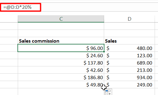
Когда динамический массив отсутствовал, в Excel происходило нечто, называемое неявным пересечением, которое заставляло возвращать один результат, даже если формула могла возвращать несколько результатов. Рассмотрим пример: если формула = B: B * 5% применяется в Excel 2019 или более ранних версиях с неявным пересечением, результат будет следующим:
Однако, когда та же формула используется в Excel 365, вы видите следующую ошибку
Чтобы решить эту проблему, попробуйте следующие исправления
Исправление 1: примените неявное пересечение с помощью оператора @
Когда мы говорим = B: B, динамический массив будет ссылаться на весь столбец B. Вместо этого мы можем заставить Excel наложить неявное пересечение с помощью оператора @
Измените формулу на [email protected]: B * 5%
Поскольку добавлено неявное пересечение, формула будет применена к одной ячейке. Чтобы расширить формулу,
1. Просто нажмите на точку, как показано ниже.
2. При необходимости перетащите его на ячейки. К этим ячейкам будет применена та же формула.
Исправление 2: вместо ссылки на столбец обратитесь к диапазону
В формуле = B: B * 5% мы ссылаемся на столбец B. Вместо этого ссылаемся на конкретный диапазон = B2: B4 * 5%.
Это все
Надеемся, эта статья была информативной.
Пожалуйста, поставьте лайк и прокомментируйте, если вам удалось решить проблему с помощью вышеуказанных методов.
Спасибо за чтение.
About spilling and the #SPILL! error
With the introduction of Dynamic Arrays in Excel, formulas that return multiple values «spill» these values directly onto the worksheet. The rectangle that encloses the values is called the «spill range». When data changes, the spill range will expand or contract as needed. You might see new values added, or existing values disappear.
Video: Spilling and the spill range
Spill behavior is native
It’s important to understand that spill behavior is automatic and native. In Dynamic Excel (Excel 365/2021) any formula, even a simple formula without functions, can spill results. Although there are ways to stop a formula from returning multiple results, spilling itself can’t be disabled with a global setting. Similarly, there is no option in Excel to «disable #SPILL errors. To fix a #SPILL error, you’ll have to investigate and resolve the root cause of the problem.
Spill error information
A #SPILL error often occurs when a spill range is blocked by something on the worksheet. Sometimes this is expected. For example, you have entered a formula, expecting it to spill, but existing data in the worksheet is in the way. The solution is just to clear the spill range of any obstructing data. Less often, a #SPILL error has another cause. You can click the spill error indicator to see more information about the cause of the error:

Read below for more information about #SPILL! errors and the specific fixes.
1. Spill range blocked
This is the simplest case to resolve. The formula should return multiple values, but instead it returns #SPILL! because there is already something in the spill range. In the screen below, the «x» is blocking the spill range:

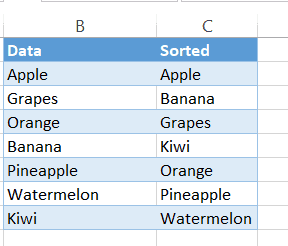
To fix the error, select any cell in the spill range so you can see its boundaries. Then make sure all cells in the spill range are empty. Once the «x» is removed, the UNIQUE function spills results normally:

Cells in the spill range must be empty, so be alert to cells with invisible characters, like spaces.
2. Excel Tables do not support dynamic arrays
Dynamic array formulas are not compatible with Excel tables. If you try to add a dynamic array formula to an Excel Table, the formula will return a #SPILL! error in all rows. The solution in this case is to (1) use an alternative formula or (2) remove the Excel Table by converting it to a normal range with the Convert to Range button on the Table Design tab of the Ribbon: Table Design > Convert to Range
Video: How to remove an Excel Table.
3. Spill range is unknown
Some functions are volatile and can’t be used with dynamic array functions because the result would be «unknown» and dynamic formulas do not currently support arrays of unknown length. For example, the following formula will return a #SPILL! error:
=SEQUENCE(RANDBETWEEN(1,100))
This happens because RANDBETWEEN is volatile and the array returned by SEQUENCE would therefore have an unknown length. The only solution is to avoid dynamic array formulas that create arrays or ranges of an unknown length.
4. Spill range too big
It is possible to write a formula that creates a spill range that extends off the edge of the worksheet. For example, the following formula uses the full column reference A:A:
=A:A+1
If this formula is entered in any row except row 1, it will return a #SPILL! error with a «Spill range is too big» message. This happens because the resulting spill range includes 1,048,576 rows (the limit in Excel) and will run off the bottom of the worksheet. Similarly, the formula below tries to use SEQUENCE to create an array with 17,000 columns:
=SEQUENCE(1,17000)
Because an Excel worksheet contains only 16,384 columns, this formula also returns a #SPILL! error. The solution is to avoid references and formulas that may create spill ranges that do not fit on the worksheet.
5. Implicit intersection (@)
Before Dynamic Arrays, Excel silently applied a behavior called «implicit intersection» to ensure that certain formulas with the potential to return multiple results only returned a single result. In non-dynamic array Excel, these formulas return a normal-looking result with no error. However, in certain cases the same formula entered in Dynamic Excel may create a #SPILL error. For example, in the screen below, cell D5 contains this formula, copied down:
=$B$5:$B$10+3

This formula would not throw an error in Excel 2016 because implicit intersection would prevent the formula from returning multiple results. However, in Dynamic Excel, the same formula automatically returns multiple results that crash into each other, since the formula is copied down in D5:D10. One solution is to use the @ character to enable implicit intersection like this:
= @$B$5:$B$10+3
With this change, each formula returns a single result again and the #SPILL error disappears.

Note: this also explains why you might suddenly see the «@» character appear in formulas created in older versions of Excel. This is done to maintain compatibility. Since formulas in older versions of Excel can’t spill into multiple cells, the @ is added to ensure the same behavior when the formula is opened in a version of Excel that supports dynamic arrays.
A better way to fix the #SPILL error above is to use a native dynamic array formula in cell D5:
=B5:B10+3
In Dynamic Excel, this single formula will spill results into the range D5:D10, as seen in the screen below:

Note there is no need to use an absolute reference since one formula creates all six results.
Note: This tutorial on how to fix the Excel spill error is suitable for Excel versions included in Office 365.
The # Spill Excel error, commonly referred to as the spill error is a commonly encountered Excel issue affecting many users who use Office 365 versions of Excel.
In this tutorial, I’ll walk you through some important methods to troubleshoot this error.
You’ll learn:
Table Of Contents
- What Does Spill Mean in Excel?
- What Causes the Spill Error in Excel?
- How to Fix the Spill Error in Excel?
- Spill Range Is Not Blank
- Spilling Inside Tables
- Spill Range Contains Merged Cells
- Spill Range is Unknown
- Spill Range is Too Big
- FAQs
- How do I turn off spill in Excel?
- How do I fix the Vlookup spill error?
- Closing Thoughts
Related:
How to Superscript in Excel? (9 Best Methods)
How to Enable Excel Dark Mode? 3 Simple Steps
How to Shade Every Other Row in Excel? (5 Best Methods)
What Does Spill Mean in Excel?
Before we proceed to look at all the methods to fix the Excel spill error, we need to first understand what ‘spill’ means in Excel.
The latest version of Excel in the Office 365 subscription, comes with a set of formulas that support dynamic arrays. This means that these formulas can do multiple calculations and return multiple values at the same time, unlike a normal Excel formula.
In case there are multiple results, they are filled up in the adjacent cells to the formula cell. This is called ‘Spilling’ in Excel.
What Causes the Spill Error in Excel?
In most cases, the reason is very simple. Some values might already be present in the spill range of a dynamic array function. This will create a conflict and Excel will alert you with a #Spill Error.
But, in some cases, the reasons are not so obvious.
There might be other reasons as well, like invisible values blocking the spill range, dragged formula blocking the spill range, or unsupported or improper use of dynamic arrays etc.
You have to look at each such error carefully to determine what is causing the problem.
Also Read:
How to Apply the Accounting Number Format in Excel? (3 Best methods)
How to Autofit Excel Cells? 3 Best Methods
The FORMULATEXT Excel Function – 2 Best Examples
How to Fix the Spill Error in Excel?
To fix the fill error in Excel, first identify the error message displayed by clicking on the yellow warning triangle inside the error cell.
Then follow the steps provided, for your corresponding error message.
Spill Range Is Not Blank
This means that some value or formula is obstructing the spill range of your dynamic array formula. To fix the error, follow these steps:
- Clear the entire spill range after the dynamic array formula.
- Or move the dynamic array formula to another location.
- If the spill range is visibly clear, but still causing spill error, click on the Select Obstructing cells option below the error message. This will highlight the cells that are obstructing the spill range. Delete them to remove the error.

- Please keep in mind that dynamic array formulas should not be dragged in the spill range direction.

Spilling Inside Tables
Please keep in mind that dynamic array formulas are not supported in Excel tables. This error means that this is the case. To fix this, either move the formula to another location or format the table as ranges.
Spill Range Contains Merged Cells
This means that one or more merged cells are obstructing the spill range. To fix this error, unmerge the merged cells or delete them. If you cannot visually locate them, click on the Select Obstructing cells option to select them.
Spill Range is Unknown
This error message means that you are using a combination of two or more dynamic array functions in the format Function1(Function2()).
Here, Function1 cannot determine the size of the spill array returned by Function2. This means that Function2 is volatile.
To fix this problem, you have to replace this volatile function with a better alternative or find some other way to do the task without using it.
Spill Range is Too Big
This means that your dynamic array function returns a spill array whose length extends beyond the edges of your Excel spreadsheet. (1,048,576 rows)
This can happen due to many reasons. But the usual cause is a poor choice of formula, where columns are used as reference instead of ranges of cells.

To fix this, either use ranges or cells as references inside the formula. But note, this will make the dynamic array formula into a normal formula.

To keep using the dynamic formula, use an implicit intersection inside the formula by adding “@” in front of the column reference that is causing the problem.
An implicit intersection is a fancy way of asking Excel to force multiple values into a single cell value, thus fixing the Excel spill errors.
Suggested Reads:
How to Use the Format Painter Excel Feature? — 3 Bonus Tips
How to Delete a Pivot Table in Excel? 4 Best Methods
How to Sort a Pivot Table in Excel? 6 Best Methods
FAQs
How do I turn off spill in Excel?
To turn off spill in Excel, insert the symbol ‘@’ before the formula that is causing the error. This will turn on the implicit intersection feature, i.e it will automatically reduce multiple values to a single value.
How do I fix the Vlookup spill error?
Excel Spill Errors in Vlookup are usually caused by using columns as a reference inside the VLOOKUP formula. Change all such references to normal range references. This will usually fix the Spill Error.
Closing Thoughts
In this tutorial, we saw what causes Excel spill errors. I have explained the various methods to fix these errors using examples. Keep these things in mind, as they will come in handy anytime.
If you have any questions about this or any other Excel feature, please let us know in the comments section.
You can find more high-quality Excel guides here.
Ready to dive deep into Excel? Click here for advanced Excel courses with in-depth training modules.
Simon Sez IT has been teaching Excel and other business software for over ten years. For a low, monthly fee you can get access to 100+ IT training courses.

Simon Calder

Chris “Simon” Calder was working as a Project Manager in IT for one of Los Angeles’ most prestigious cultural institutions, LACMA.
He taught himself to use Microsoft Project from a giant textbook and hated every moment of it. Online learning was in its infancy then, but he spotted an opportunity and made an online MS Project course — the rest, as they say, is history!
![]()
Excel #SPILL! Error
More and more Excel users are encountering an error they have never seen before called #SPILL!.
This begs two questions:
- What exactly is a #SPILL! error?
- How do I get it to go away?
The reasons for its existence can sometimes be crystal clear while other times more opaque.
Let’s learn exactly what the #SPILL! error is and how to deal with it.
")
What is the #SPILL! Error?
The #SPILL! error is a product of the new Dynamic Array calculation engine in use by Excel for Office 365 subscribers.
Historically, a formula would return a single result to a cell, such as calculating the SUM of a range of cells.
=SUM(A1:A10)

If we were to reference a range of cells (ex: =A1:A10), the results would be limited to the first encountered cell reference (A1).

This is because the formula is trying to display the contents of 10 cells within the confines of a single cell. Excel says to itself, “I can’t show ten results, so I’ll just show the first one.”
In the “old days” this issue was solved using array notation (CTRL-Shift-Enter) and cell pre-selection. Trust me, it’s not a road you want to go down.
With the new Dynamic Array engine, if a formula returns multiple results, the results are “spilled” into the adjacent cells.

This allows for multiple results to be displayed without the need for array notation.
All the new Dynamic Array functions utilize this spilling feature:
- SEQUENCE
- FILTER
- TRANSPOSE
- SORT
- SORTBY
- RANDARRAY
- UNIQUE
- XLOOKUP
- XMATCH
The spilling feature has also carried over to the traditional function library for use by functions such as SUM, MATCH, and FREQUENCY.

Master Excel Functions in Office 365 & Office 2021 — Complete Course
Excel has Changed Forever! DON’T MISS OUT!
What Happens If I Can’t Spill?
One of the requirements for the spill behavior to operate properly is that there must be an area of unoccupied cells for which to spill into.
If you are trying to display 10 results, but there is data in any of the 10 needed cells, Excel will respond with a #SPILL! error message.

The dotted-blue border indicates the area that is needed to display the results.
To solve this problem, either move or delete the data located in the spill range.

If you are uncertain where the obstruction lies, you can select the Error “floatie” (exclamation button) and click “Select Obstructing Cells” to have attention drawn to the offending cell(s).

This is especially useful for situations where you may need to spill into hundreds or thousands of cells. Selecting each cell in the spill range to look for anomalous data would be impractical.
Not-so-Obvious Errors
Sometimes, the reason for a #SPILL! error is not as obvious as the example above.
An easy example is text that has been formatted with the same font color as the cell’s fill color.

Custom Number Formatting can also play a part in hiding text. Take for example the following number format code set.
; ; ;

This is a sneaky way to hide anything placed in a cell, regardless of font color or cell color.
The three semi-colons are saying, “Show no positive numbers, show no negative numbers, show no zeroes, and show no text.”
If you wish to learn more about Custom Number Formatting, check out these posts:
Learning Excel Custom Number Formatting
Why you SHOULD be USING Custom Number Formatting
Complete Course: Excel Functions in 365
Confused about the NEW Excel Functions? Spill Errors and What Dynamic Arrays mean?
In my EXCEL DYNAMIC ARRAYS COURSE we cover it all!
You’ll master these functions through multiple exercises and challenges so you can use the FILTER Function instead of a complex combination of INDEX & MATCH.
Or use XLOOKUP instead of VLOOKUP.
Not only will these save you from headaches but also from wasting time doing things the long way.
Get access to the Course HERE.

Other Reasons for #SPILL!
There are some more exotic reasons for why the #SPILL! error can occur. The previously mentioned reasons are the most common, but here are other reasons you may wish to investigate if the obvious fails.
Indeterminate Size
Excel was unable to determine the size of the spilled array because it’s volatile and resizes between calculation passes. For instance, the following formula will trigger this #SPILL! error:
=SEQUENCE(RANDBETWEEN(1, 1000) )
Dynamic array resizes may trigger additional calculation passes to ensure the spreadsheet is fully calculated. If the size of the array continues to change during these additional passes and does not stabilize, Excel will resolve the dynamic array as #SPILL!.
Results Extend Beyond the Worksheet’s Boundary
For example, if we placed in cell B2 the following formula…
=VLOOKUP(A:A, A:C, 2, FALSE)
The results would cause a #SPILL! error because Excel will lookup the entire column, return 1,048,576 results, and hit the end of the Excel grid. So close; we only needed one more cell.
It’s generally considered poor practice to select entire columns when selecting ranges.
Table Formulas
Spilled array formulas are not supported in Excel Tables. Spilled formulas should only exist in a single cell. Excel Tables will repeat the formula to every cell in the table’s column. This creates catastrophic interference between every cell in the column.

If you need to use the formula as a spilled array formula, you will need to revert the Excel table to a “plain table” using the Table Design (tab) -> Tools (group) -> Convert to Range option.
Out of Memory
The spilled array formula you’re attempting to enter has caused Excel to run out of memory. In these cases, try referencing a smaller array or range.
Spilling into Merged Cells
If the results of the spilled array encounter a cell that has been merged with other cells, a #SPILL! error will occur.

Unrecognized / Fallback
If Excel doesn’t recognize or can’t reconcile the cause of this error, make sure your formula contains all the required arguments for your scenario.
Practice Workbook
Feel free to Download the Workbook HERE.
![]()
COMPLETE Course about Excel Functions in 365 & Office 2021
Master the NEW Excel Formulas
FILTER, SORT, UNIQUE: From Beginner to Expert Level!
If you’re using Excel 365 or newer versions, you might have come across the SPILL error.
This is a new error code that you will find in addition to the usual error codes in Excel 365.
In fact, although the term SPILL is new, the behavior of spilling is something that dynamic array functions have been demonstrating in earlier Excel versions too.
In this tutorial, we are going to uncover what the SPILL error means, why you might find a SPILL error code in your worksheet and how to get rid of it.
What Does it Mean to SPILL in Excel
If you’ve used dynamic array functions before, the ‘spilling’ behavior might be familiar to you.
When you use dynamic array functions like SORT, UNIQUE, FILTER, etc. in Excel, you get an array in return, instead of a single value.
The array consists of a set of values that need to occupy a group of cells. This behavior of returned values covering more than one neighboring cell(s) is called ‘spilling’.
For example, in the following screenshot, the SORT function returns an array of 9 values, even though we’ve entered the formula in a single cell (B2).

All the 9 returned values simply ‘spill’ into the range B2:B10.
We call this range of cells (B2:B10) that hold the returned array the ‘spill range’.
What is a SPILL Error in Excel?
A SPILL error is an error that occurs when there is something in your worksheet that is preventing an array formula from spilling properly.

In the above image, the value 5, which is in the spill range of the SORT function is preventing the results from spilling into the range.
This is causing a SPILL error, due to which we can see the #SPILL! error code in cell B2.
Note: When you click on the cell containing the formula, you can see its spill range surrounded by dotted lines, as shown in the above screenshot.
The SPILL error mainly occurs when your dynamic array formula’s results are not able to spill into its designated spill range.
There may be multiple reasons preventing your formula from spilling.
Sometimes they’re visible, as can be seen in the above screenshot, and sometimes they’re not all that obvious.
So, if you want to resolve a SPILL error, you need to first diagnose the cause.
Let us look at some common causes of the SPILL error, and how to correct each of them.
Possible Reasons for a SPILL Error in Excel
Here are some possible reasons for a SPILL error:
- The SPILL range may have certain cells containing content (that may or may not be visible to us)
- The SPILL range may contain merged cells
- The SPILL range may be a part of an Excel Table
- The SPILL range may be indeterminate
- The SPILL range may be larger than the space available
A good way to narrow down the reason is by clicking on the warning icon (or green triangle) next to the #SPILL! error code.
Doing this will display the possible cause in the first line of the popup, as shown below:

Let us explore each of the possible causes along with ways to solve them.
Problem: SPILL Range Isn’t Blank
Excel does not allow the dynamic array functions to overwrite non-blank cells with their returned array.
So the function simply returns a SPILL error.
Solution: Clear the SPILL Range
The solution, in this case, is to simply remove the contents from the non-blank cell(s) that are within the spill range.
When you select the formula, you will notice a dashed border around the area of the spill range.
If you see any content within this range, simply remove it or move it to some other cell that is outside the spill range.
Doing this clears the spill area out, so that the function can display its returned results in its spill range.
Sometimes there may be content in some of the spill range cells but they may not be visible.
For example, the font may be of the same color as the cell background. This may get the contents camouflaged.
In such cases, simply select all the cells in the spill range and change font color to Automatic or navigate to Cell Styles -> Normal from the Styles group.

Your hidden cell contents should now be visible.
You can then choose to remove or shift these contents so that your formula can now spill its results in the spill range.
One common scenario is where you may see the SPILL error even when there is no content in the range where the formula result is supposed to come. This could happen if there are cells with space characters. While the space character won’t be visible to you, it will stop the formula to show the result. To correct this, select all the cells in the range and hit delete
Problem: SPILL Range Contains Merged Cells
If any of the cells in your spill range are merged or are part of a merged cell, then your formula cannot spill its results.

Solution: Unmerge the Cells in the SPILL Range
The solution to this problem is to simply unmerge the cells by selecting them and navigating to Home -> Merge & Center -> Unmerge.

Alternatively, you can move the merged cell to some other location that is outside the spill range.
Problem: SPILL Range is in Table
Excel tables don’t support spilled array formulas.
So if your spill area contains a table, or if one or more cells in your spill area happen to fall in an Excel table, you are going to get a SPILL error.

Solution: Convert the table back to a normal range or shift the formula to an area outside the table.
To resolve this, simply move your formula so that its spill area doesn’t fall into the area of the table.
Alternatively, you can convert the table back to a regular range by selecting it and navigating to Table Design ->Tools->Convert to Range.

Problem: SPILL Range is Unknown
When you use volatile functions in your formula, like the RAND, RANDARRAY, and RANDBETWEEN for example, it becomes difficult for Excel to determine the size of the spilled array.
This may be because the array keeps resizing on every calculation pass, causing your result to destabilize.
For example, in the screenshot shown below, the RANDBETWEEN function keeps recalculating, causing the SEQUENCE function to return arrays of different sizes between each calculation pass.
This results in a SPILL error:

Solution: Fix the formula
You can resolve this error by fixing your formula, making sure the volatile function in it returns a determinable and fixed-sized array.

Problem: SPILL Range is too Big
If you refer to entire columns instead of a range containing a subset of columns, you are likely to get a SPILL error.
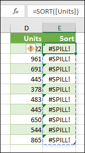
For example, say you want to use the formula =SORT(A:A) to sort all numbers of column A and display the result as a spilled array in cell B2. Using this formula in Office 365 and later versions returns a SPILL error:

This is because the range A:A is referring to all the thousand or so cells of your column A.
This makes your returned array spill over the edge of your spreadsheet since your formula starts at row 2 (of column B).
This means your spill range is bigger than the number of cells available.
Solution: Avoid Using Column References or move the Formula to the Top of the Column
To resolve this issue, either use references to just the subset of cells containing your data (A2:A10) or move your formula up to the first cell of your column.
In general, when using dynamic array functions, it is always better to steer clear of using entire column references.
In this tutorial, we showed you some possible reasons for getting SPILL errors in Excel.
We also showed you how to find out what’s causing the error and different ways to resolve it.
We hope this helps you in diagnosing and fixing your SPILL errors, if any, in Excel.
Other Excel tutorials you may also find helpful:
- Can’t Type In Excel: 6 Possible Reasons and Solutions!
- Why is Merge and Center Grayed Out?
- Why does Excel Open on Startup (and How to Stop it)
- How to Remove Read-Only From Excel (6 Easy Fix)
- How to Find out What Version of Excel You Have
- #NUM Error in Excel – How to Fix it?
- Subscript Out of Range Error in VBA
#SPILL! error in Excel is most commonly experienced while using a dynamic array function. A formula that cannot fill the required cells with the calculated results creates this error.
After the introduction of dynamic arrays, the formulas can often return multiple values. In such cases, the result will be «spilled» in the worksheet, and the cell range is known as the «spill range».
The most common scenario of the #SPILL! error is when there is a spill range blockage or the reference used for the formula is beyond the limits of the worksheet.
In this tutorial, we’re going to walk you through what the #SPILL! error is, why it occurs, and the ways to fix it.
What is a #SPILL! Error in Excel?
A #SPILL! error typically happens when a formula generates several results but cannot output them on the worksheet. To better understand the error, you must first understand the terms such as ‘spilling’ and ‘spill range’. Along with the cell obstruction case, there are several other cases where you might face the #SPILL! error in Excel.
We are quite accustomed to entering a formula, receiving the result in the same cell, and then extending that formula by click-and-drag. But what would happen if only one entered formula is to produce more than one result?
The term «spill» describes the behavior in which formulas that yield numerous results automatically «spill» their results into numerous cells. The result will be spilled in the worksheet taking up the required number of cells to display the result. E.g. if one formula needs 5 cells to display its result, it will fill 5 cells including the cell the formula is in.
The range of values that an array formula returns and spills into a worksheet is called the «spill range».
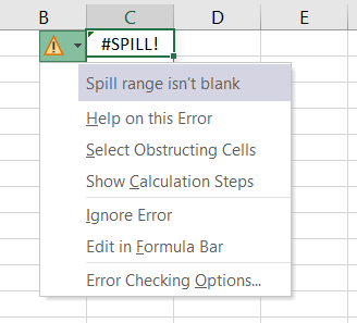
It is usually highlighted with a dashed blue border. Excel also helps you understand what went wrong with your formula. If your formula brings about an error, selecting the cell will display an error icon. Click this icon to get help with the error along with access to more options on handling the error.
Reasons for #SPILL! Error in Excel
Below mentioned are several possible causes of #SPILL! error along with their fixes.
1- Spill Range is Obstructed
This is one of the most common and basic cases of #SPILL! error. There is no space on the worksheet to show the return values. For example, if the formula is expected to return two values, but only one neighboring cell is available, it will give a #SPILL! error.
The error will vanish after removing the obstruction, and the range will be filled with the predicted formula results.
Example 1 – Spill Range is blocked
In our example, we have a list of names that are split into first and last names in columns A and B. If we are to re-organize the data from a vertical to horizontal set, one way to do that is to use the TRANSPOSE function. This formula would do for transposing the list in column A to row 1:
=TRANSPOSE(A2:A7)
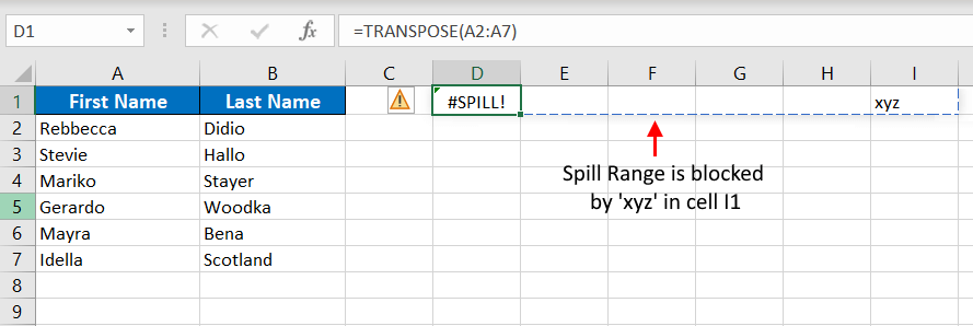
To rearrange the data, we’ve supplied the TRANSPOSE function with the range A2:A7 containing the first names in column A. The formula is entered in cell D1. With 6 names in column A, the formula will need 6 cells to display and spill the result i.e. from D1 to I1.
However, because there is data in cell I1, the spill range is blocked. Hence the #SPILL! error.
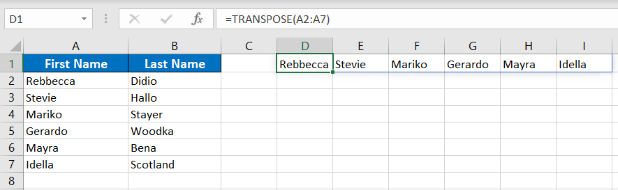
Solution 1:
The first instinctive solution for this #SPILL! error is to remove the obstruction which is to delete or move the data from I1. When the data is deleted, the result of the formula will spill to I1 – #SPILL! error taken care of!
However, it may not always be possible or convenient to get rid of the data and so you have another option to fix this error.
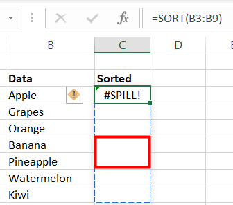
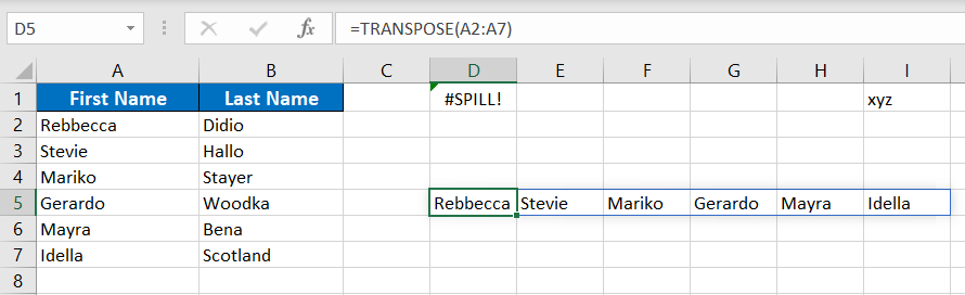
Solution 2:
The other solution is to relocate the target cell of your formula. Since the spill range ahead of D1 has a non-blank cell, there is no issue in this scenario to move the formula a few cells down. Therefore, we have shifted our target cell from D1 to D5 which allows the result to spill freely to I5.
There can be several other instances where you might face a similar issue. The blocked spill range can be due to value, a special character, an invisible character, or a cell with a formula returning an empty value.
Example 2 – Invisible Obstruction
As compared to a blocked cell that we can clearly see, the error could be due to a blocked cell, that is not visible. This can be because of the font color, or because the cell data is formatted to make the cell value disappear using the custom format ;;; via the Format Cells dialog box.
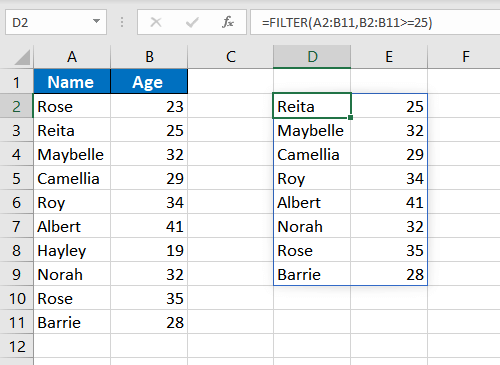
For the example below, we have the ages of a group of people and are using the formula ahead with the FILTER function to list down the people aged 25 and above:
=FILTER(A2:B11,B2:B11>=25)
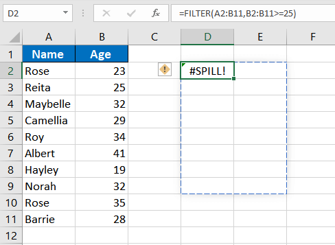
The formula is giving a #SPILL! error, but there is no visible obstruction.
Solution:
To fix it, click on the Error floatie and choose «Select Obstructing Cells«. It will highlight the cells where there is data. D7 shows the text “Block”, but we cannot see it.
It is because the font is white. Remove the data, and the error is fixed.
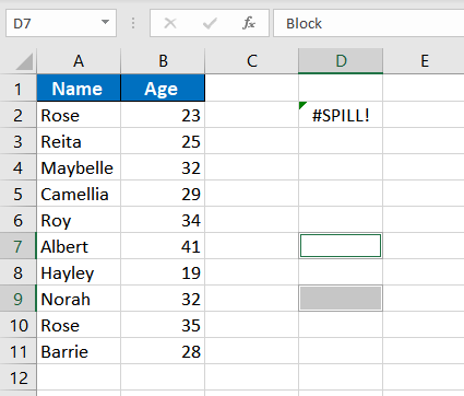
Similarly, cell D9 shows the text ‘Block 2’ with the font color black, but we are still unable to see it. It is because the cell is formatted to disappear. To check, right-click on the cell and select Format Cells. is «;;;» If in the Number tab, you find that the Custom category is selected with ;;; in the Type box, it is a formatted cell whose value is formatted to be invisible.
The solution is simple; either delete the value or shift the formula where there is enough space for the spill range.
2- Merged Cell in Spill Range
The #SPILL! error in Excel is also experienced if the spill range includes a merged cell. Click on the warning flag and look at the cause, «Spill range has a merged cell» to make sure that the merged cells are to blame for the problem.
Example – Spill Range includes merged cell
The example we have here has a list of products with their respective categories. To get the final range of the categories, the formula below with the UNIQUE function can be used:
=UNIQUE(B2:B10)
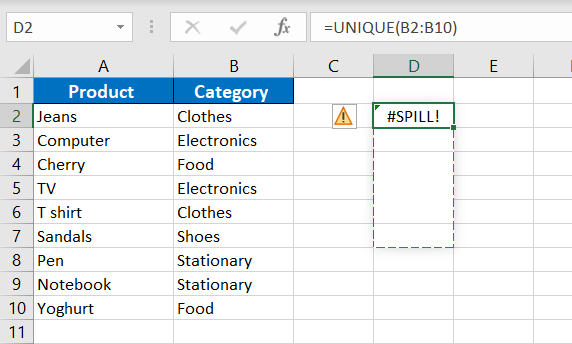
Using this formula with B2:B10 as the given range, we are trying to find unique values in the category column. There is a #SPILL! error because D4 is merged with D5 and D6; a part of the spill range.
Solution
Unmerge the cells in the spilling space by selecting the merged cell and going to the Home tab > Alignment group > Merge & Center button. If you have large data, click on the error symbol, select the Obstructing Cells option to automatically locate the problem cells, and then unmerge the problem cell.
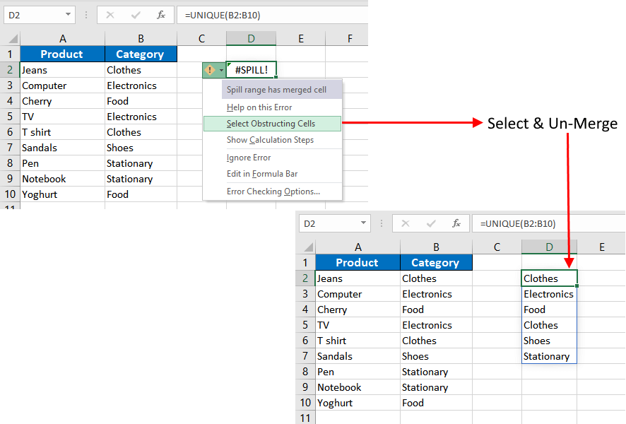
No merged cell – no problem; the #SPILL! error will be solved as the merged cell will be gone.
3- Spill Range is Undetermined
Dynamic Array formulas when combined with volatile functions such as RAND, RANDARRAY, RANDBETWEEN, etc., result in the #SPILL! error. This is because volatile functions cause frequent recalculation.
Hence, the dynamic array formula cannot define the spill range. This will cause Excel to show ‘Spill Range is Unknown’ as the error description using the error icon.
Example – Using SEQUENCE & RANDBETWEEN
The following formula generates a #SPILL! error:
=SEQUENCE(RANDBETWEEN(1,300))
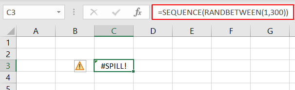
Since the result of RANDBETWEEN varies frequently with every recalculation on the sheet, the SEQUENCE function, which is to return numbers in sequence, is unsure of how many values to produce. Therefore, the spill array is unknown/can’t be determined and so Excel gives us a #SPILL! error.
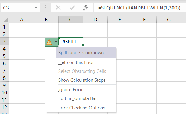
By checking the «Spill range is unknown» cautionary indicator, you can verify the error’s root cause.
Solution
Sadly, the solution is to use a different formula. You can use alternative formulas that produce arrays or ranges with defined lengths.
4- Spill Range is Beyond the Limits of Worksheet
When using a formula that might return too many values for the worksheet, it will return a #SPILL! error. In such cases, the formula’s spill range is such that it would extend outside the borders of the worksheet. It can be better understood using examples.
Example 1 – The spill range is big
For the employees in this example, we are trying to increase everyone’s salary by 10%. This should be achievable with a simple formula like the one below:
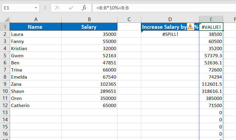
=B:B*10%+B:B
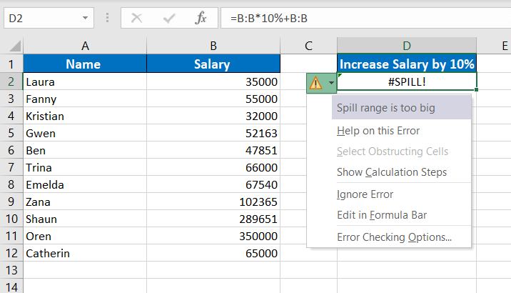
Here, column B refers to the salary column and the idea is to increment the whole column by 10%. It gives a #SPILL! error because the spill range is more than the rows in Excel. Excel contains 1048576 rows. To return the calculation on an entire column, column B in our case, the formula will require 1048576 rows.
We are using the formula in D2 and the formula will need the 1048577th row to display the complete result. Since Excel doesn’t have rows beyond 1048576, this means that the spill range will go beyond the worksheet. That is not possible, creating the #SPILL! error.
Solution 1:
If we use the same formula in E1, it will spill the required result. You are getting a #VALUE! error because it is also trying to calculate the value of B1 which is not a numeric value.
Solution 2:
Instead of referring the whole column B:B, you can define the range that column B covers in the dataset as B2:B12 and use this formula instead:
=B2:B12*10%+B2:B12
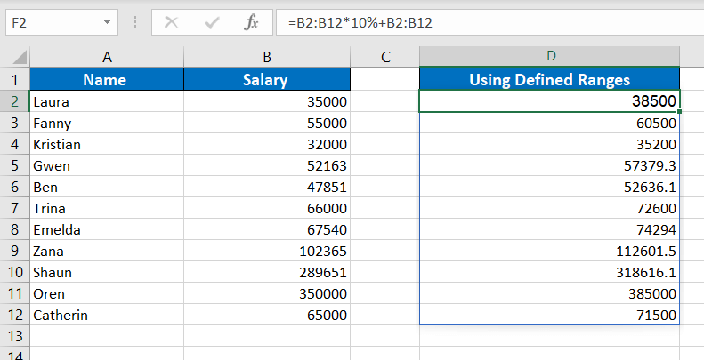
This formula will result in a spilled range from the target cell D2 to D12.
Solution 3:
Use only the cell reference of the first row of the dataset (that is row 2 for us. For column B, the first data cell for the formula will be B2), then using the fill handle, copy the formula to your required range.
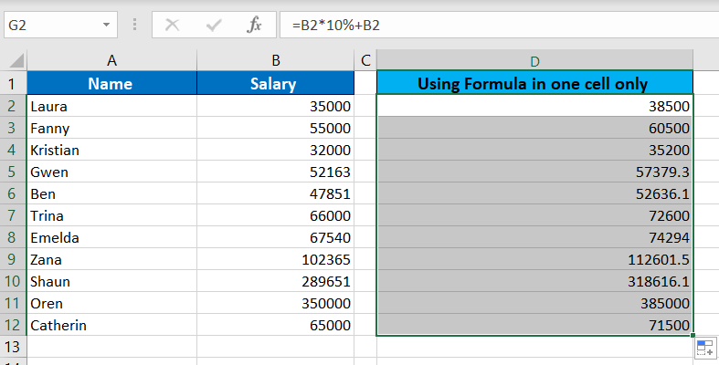
Use the formula in D2 using the reference of cell B2 only. Then drag to duplicate it to D12.
Example 2 – Implicit intersection (@)
Implicit intersection operator «@» converts an array or range to a single value. If a function exceeds the spill range to the edge of the worksheet, use «@» to convert it to a single value. Then drag and copy the formula to the remaining cells.
In the example, we are using the VLOOKUP function through this formula:
=VLOOKUP(A:A,A:B,1,FALSE)
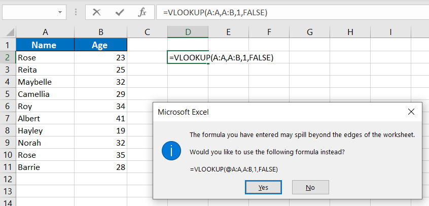
Ideally, the function will look up cell A2; but since the column reference we’ve used is A:A, it will look up the entire column A, making the spill range exceed the worksheet space. Excel itself will give an error and suggest you use ‘@’.
When you accept the suggestion by the prompt, it adds the implicit intersection operator and returns the value of A2 (the particular row where the formula is written). You can then drag the formula to fill and complete your range.
Example 3 – Results spilling beyond the worksheet column limits
There are 1,048,576 rows and 16,384 columns in Excel. If you use a formula that spills beyond the sheet, it will give a #SPILL! error.
=SEQUENCE(1,16385)
If you use the above formula (or SEQUENCE function with any number greater than 16,384), it will result in a #SPILL! error.
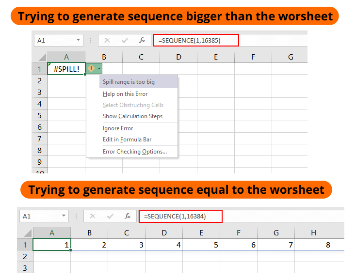
To fix this error, you can try changing the formula as:
=SEQUENCE(1,16384)
Make sure to enter it in the first column so that it will spill your sequence all the way to the last column without needing more columns.
Solution
Avoiding references and calculations that could result in spill ranges that don’t fit the worksheet or try to shift the target cell to earlier rows/columns so that the formula has enough cells for the spill range.
5- Excel Tables With Dynamic Arrays
Dynamic array does not work well with the Excel Tables. If you try to use an array formula within a table, it will result in a #SPILL! error. To verify the case, check the error symbol that shows ’Spill range in table’.
Example – Array Formula in Excel Table
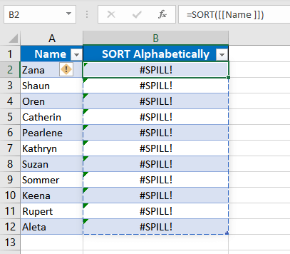
The example comprises a list of names in an Excel Table. Now we’ll use the following formula so the Name column is sorted in alphabetical order.
=SORT([[Name ]])
We have encountered the #SPILL! error again. With the target cell in selection, we can click on the error icon to confirm the reason for the #SPILL! error which is ’Spill range in table’.
Solution 1
Use the formula outside the Table referring the Table and column. Copying the formula from above, we’ve referred the Table name in the formula:
=SORT(Table1[[Name ]])
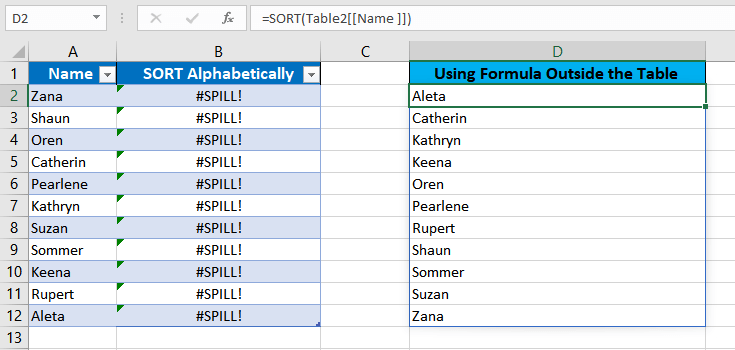
If the formula is placed in F5 instead of D5, it shows the desired results, avoiding the #SPILL! error.
Solution 2
If the Table is causing the problem, you can convert the Table into a range. All you need to do is right-click any cell in the Excel Table, hover the cursor on the Table option in the context menu, and select Convert to Range.
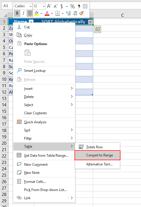
Now that the Table element is gone, we’re working with a regular range. The formula ahead will not result in a #SPILL! error and will also sort the names alphabetically:

Apart from the scenarios mentioned above, you might face the #SPILL! error in Excel if it runs out of memory. In that case, try using smaller ranges.
Hopefully, now you will be able to resolve the #SPILL! error in all the possible conditions. While you solve your #SPILL! errors, we’ll bring you some more tutorials to make sure your Excel rides are buttery-smooth.