Expected calibration error

07 Aug 2020

Predictions are not just about accuracy, but also about probability. In lots of applications it is important to know how sure a neural network is of a prediction. However, the softmax probabilities in neural networks are not always calibrated and don’t necessarily measure uncertainty.

In this blog post, I will implement the most common metrics to evaluate the output probabilities of neural networks.

There are in general two types of metrics:

1. Proper scoring rules estimate the deviation from the true probability distribution. A high value indicates that the predicted probability (0 leq hat{p} leq 1) is far away from the true probability (p in {0, 1}). Whether (hat{p}) equals (0.6) or (hat{p}) equals (0.8) is not as important as the distance from (1) or (0).
2. Calibration metrics measure the difference between “true confidence” and “predicted confidence”. If (hat{p}) equals (0.6), then it should mean that the neural network is 60% sure. A model is calibrated if (mathbf{P}left(hat{Y} = y mid hat{P} = pright) = p). Then the difference is (leftlvert mathbf{P}left(hat{Y} = y mid hat{P} = pright) — prightrvert). The predicted confidence is the output probability of the neural network, while the true confidence is estimated by the corresponding accuracy. Calibration metrics are computed on the whole dataset in order to group different probabilities (e.g. 0% — 10%, 10% — 20%, …). In contrast, proper scoring rules compare individual probabilities.

14/08/20 update: added recommendations, static calibration error and thresholding

30/08/21 update: the traditional reliability diagram, as it is known from weather forecasts, has the relative frequency and not the accuracy on the y-axis. However, papers like “On Calibration of Modern Neural Networks” have the accuracy on the y-axis. I use the latter convention here but would recommend the traditional definition as it gives better results.

Proper scoring rules

Negative log likelihood

Negative log likelihood (NLL) is the usual method for optimizing neural networks for classification tasks. However, this loss function can also be used as a uncertainty metric. For example, the Deepfake Detection Challenge scored submissions on NLL.

[H(p, hat{p}) = -mathbf{E}_{p}[log hat{p}] = -sum_{i=1}^n p_ilogleft(hat{p}_iright) = -logleft(hat{p}_jright)]

where (p_j = 1) is the ground truth and (hat{p}_j = text{softmax}_jleft(xright)). PyTorch’s CrossEntropyLoss applies the softmax function and computes (H(p, hat{p})).

import torch.nn as nn

loss_func = nn.CrossEntropyLoss(reduction="mean")
nll = loss_func(logits, target)

We can also rewrite the code above using nll_loss. This shows more of what happens internally.

import torch
import torch.nn.functional as F

logits = torch.exp(logits - torch.max(logits, dim=-1, keepdim=True))
pred = torch.log(logits) - torch.log(torch.sum(logits, dim=-1, keepdim=True))
nll = F.nll_loss(pred, target, reduction="mean")

To ensure numerical stability (max(x)) was subtracted from (logleft(text{softmax}_jleft(xright)right)).

Brier score

The Brier score is the mean squared error of a forecast. For a single output it is defined as follows:

[BS(p, hat{p}) = sum_{i=1}^{c}(hat{p}_{i}-p_{i})^2 = 1 — 2hat{p}_{j} + sum_{i=1}^{c} hat{p}_{i}^2]

For multiple values it is possible to sum over all outputs. The code is then

def brier_score(y_true, y_pred):
  return 1 + (np.sum(y_pred ** 2) - 2 * np.sum(y_pred[np.arange(y_pred.shape[0]), y_true])) / y_true.shape[0]

y_true should be a one dimensional array, while y_pred should be a two dimensional array. When predicting multiple classes, sometimes each class is considered individually (one-vs.-rest / one-against-all strategy).

Calibration metrics

Expected calibration error

[begin{aligned}
ECE &= mathbf{E}_{hat{P}}left[leftlvert mathbf{P}(hat{Y} = y mid hat{P} = p) — prightrvertright]\
&= sum_{p} mathbf{P}(hat{P} = p) leftlvert mathbf{P}(hat{Y} = y mid hat{P} = p) — prightrvert
end{aligned}]

We approximate the probability distribution by a histogram with (B) bins. Then (mathbf{P}(hat{P} = p) = frac{n_b}{N}) where (n_b) is the number of probabilities in bin (b) and (N) is the size of the dataset. Since we put (n_b) probabilities into one bin, (p) is not a single value. Therefore, a representative value (p = sum_{hat{p_i} in b} frac{hat{p_i}}{n_b} = text{conf}(b)) is necessary. Similarly, we can set (mathbf{P}(hat{Y} = y mid hat{P} = p) = sum_{hat{y}_i in b} frac{mathbf{1}left(y_i = hat{y_i}right)}{n_b} = text{acc}(b)) where (hat{y_i}) is obtained from the highest probability (arg max). (hat{p_i}) is also the highest probability (max).

ECE is then defined as follows:

[begin{aligned}text{ECE}(B) &= sum_{b=1}^{B} frac{n_b}{N}lverttext{acc}(b) — text{conf}(b)rvert\
&= frac{1}{N}sum_{b in B}leftlvertsum_{(hat{p_i}, hat{y_i}) in b} mathbf{1}left(y_i = hat{y_i}right) — hat{p_i}rightrvertend{aligned}]

The accuracy (text{acc}(b)) is also called “observed relative frequency”, while the confidence (text{conf}(b)) is a synonym for “average predicted frequency”.

The implementation is:

def expected_calibration_error(y_true, y_pred, num_bins=15):
  pred_y = np.argmax(y_pred, axis=-1)
  correct = (pred_y == y_true).astype(np.float32)
  prob_y = np.max(y_pred, axis=-1)

  b = np.linspace(start=0, stop=1.0, num=num_bins)
  bins = np.digitize(prob_y, bins=b, right=True)

  o = 0
  for b in range(num_bins):
    mask = bins == b
    if np.any(mask):
        o += np.abs(np.sum(correct[mask] - prob_y[mask]))

  return o / y_pred.shape[0]

y_true should be a one dimensional array like np.array([0,1,0,1,0,0]), while y_pred requires a two dimensional array e.g. np.array([[0.9, 0.1],[0.1, 0.9],[0.4, 0.6],[0.6, 0.4]], dtype=np.float32). Since most papers use between 10 and 20 bins [1], I set num_bins=15. More bins reduce the bias, but increase the variance (bias-variance tradeoff).

If you have TensorFlow Probability installed, you can also use the following function (which produces the same results):

import tensorflow_probability as tfp

tfp.stats.expected_calibration_error(num_bins=15, labels_true=gt, logits=np.log(pred))

Note if pred are logits, then np.log is not necessary.

There are a few problems with the standard ECE. np.linspace will create evenly spaced bins, which are likely to be empty. In statistics, bins are often chosen so that each bin contains an equal number of probability outcomes [2]. This is called Adaptive Calibration Error (ACE) in [1].

One can change the variable b in expected_calibration_error to obtain ACE.

b = np.linspace(start=0, stop=1.0, num=num_bins)
b = np.quantile(prob_y, b)
b = np.unique(b)
num_bins = len(b)

However, the adaptivity can also cause the number of bins to decrease. At the start of a neural network I trained, there were (15) bins. After 10 epochs the number of bins reduced to (11). The sigmoid function tends to over-emphasize probabilities near (1) or (0). For example, one training run produced the bins ({0.4786461, 0.99776319, 0.99977307, dots, 0.99995485, 0.99999988, 1., 1.}).

It is also important to note that only the highest probability is considered for ECE/ACE i.e. pred_y = np.argmax(y_pred, axis=-1). [2] proposes Static Calibration Error (SCE) which bins the predictions separately for each class probability. This should be considered, when all probabilities in a multi-class setting are equally important.

[begin{aligned}text{SCE}(B) &= frac{1}{NC}sum_{c=0}^{C-1}sum_{b in B}leftlvertsum_{hat{p_i} in b} mathbf{1}left(y_i = cright) — hat{p_i}rightrvertend{aligned}]

The implementation is:

def static_calibration_error(y_true, y_pred, num_bins=15):
  classes = y_pred.shape[-1]

  o = 0
  for cur_class in range(classes):
      correct = (cur_class == y_true).astype(np.float32)
      prob_y = y_pred[..., cur_class]

      b = np.linspace(start=0, stop=1.0, num=num_bins)
      bins = np.digitize(prob_y, bins=b, right=True)

      for b in range(num_bins):
        mask = bins == b
        if np.any(mask):
            o += np.abs(np.sum(correct[mask] - prob_y[mask]))

  return o / (y_pred.shape[0] * classes)

If there are a lot of classes, adaptive SCE will assign too many bins to predictions close to 0% (e.g. 999 classes (approx 0.01), 1 class (approx 0.99)). ECE does not have the same problem, because it only evaluates the class with the highest probability. [1] suggests thresholding the predictions in this case (e.g. (10^{-3})). Change the code as follows:

...
prob_y = y_pred[..., cur_class]
mask = prob_y > threshold
correct = correct[mask]
prob_y = prob_y[mask]
...
o += np.abs(np.sum(correct[mask] - prob_y[mask])) / prob_y.shape[0]
...
return o / classes

Some other things to keep in mind are:

• optimizing ECE: using scipy.optimize it is possible to directly optimize this non-differentiable metric. However, according to [1] “ECE is very strongly influenced by measures of calibration error that adhere to its own properties, rather than capturing a more general concept of the calibration error.”
• norm: most paper use the (L_1) norm, but (L_2) is also an option.

Reliability diagram

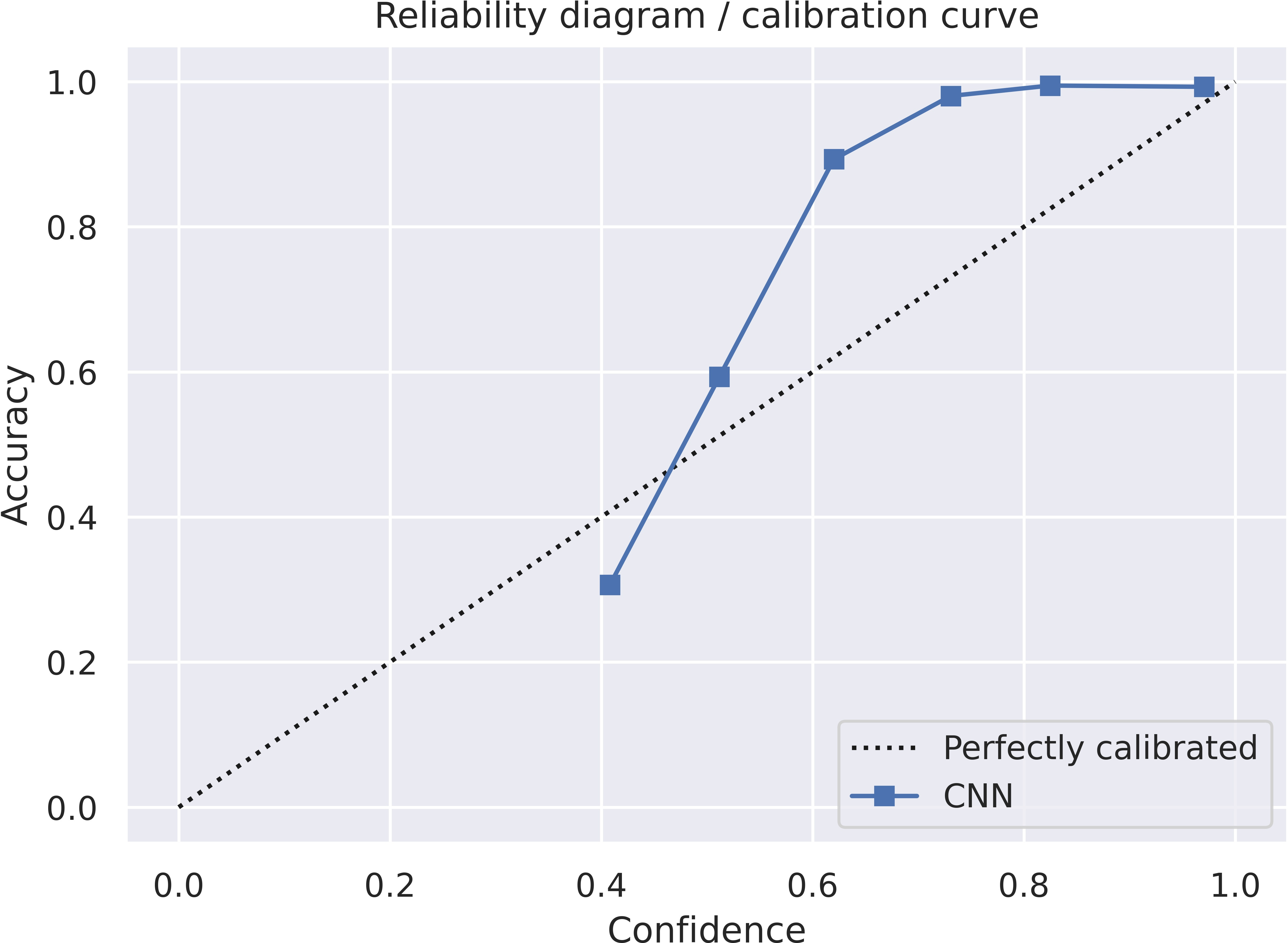
The x-axis is np.sum(prob_y[mask]) / count (confidence or avg predicted frequency) and the y-axis is np.sum(correct[mask]) / count) (accuracy). It is important to note that the traditional reliability diagram has on the y-axis the “observed relative frequency” np.sum(y_true[mask]) / count) and NOT the accuracy. I would also recommend using the “observed relative frequency” as this is the standard approach.

First, we change the function expected_calibration_error to return both values. Then the following function will produce a reliability diagram:

import matplotlib.pyplot as plt
import seaborn as sns

sns.set()

def reliability_diagram(y_true, y_pred):
    x, y = expected_calibration_error(y_true, y_pred)

    plt.plot([0, 1], [0, 1], "k:", label="Perfectly calibrated")
    plt.plot(x, y, "s-", label="CNN")

    plt.xlabel("Confidence")
    plt.ylabel("Accuracy")
    plt.legend(loc="lower right")
    plt.title("Reliability diagram / calibration curve")

    plt.tight_layout()
    plt.show()

The reliability diagram itself looks like this:

Recommendations

Using an unsuitable metric can lead to wrong conclusions. According to [3], calibration metrics should not be used to compare different models. Expected calibration error is sensitive to the number of bins and the thresholding. Furthermore, it does not provide a consistent ranking of different models.

Instead, a better metric would be BS and log likelihood provided temperature scaling was applied to the logit layer. ECE is more useful for measuring the calibration of a specific model.

References

[1] J. Nixon, M. Dusenberry et al., Measuring Calibration in Deep Learning, 2020.

[2] Hyukjun Gweon and Hao Yu, How reliable is your reliability diagram?, 2019.

[3] A. Ashuskha, A. Lyzhov, D. Molchanov et al. Pitfalls of in-domain uncertainty estimation and ensembling in deep learning, 2020.

My personal blog

Machine learning, computer vision, languages

Metrics for uncertainty estimation

Predictions are not just about accuracy, but also about probability. In lots of applications it is important to know how sure a neural network is of a prediction. However, the softmax probabilities in neural networks are not always calibrated and don’t necessarily measure uncertainty.

In this blog post, I will implement the most common metrics to evaluate the output probabilities of neural networks.

There are in general two types of metrics:

1. Proper scoring rules estimate the deviation from the true probability distribution. A high value indicates that the predicted probability (0 leq hat

   leq 1) is far away from the true probability (p in <0, 1>). Whether (hat

   ) equals (0.6) or (hat

   ) equals (0.8) is not as important as the distance from (1) or (0).

2. Calibration metrics measure the difference between “true confidence” and “predicted confidence”. If (hat

   ) equals (0.6), then it should mean that the neural network is 60% sure. A model is calibrated if (mathbf

   left(hat = y mid hat

   = pright) = p). Then the difference is (leftlvert mathbf

   left(hat = y mid hat

   = pright) — prightrvert). The predicted confidence is the output probability of the neural network, while the true confidence is estimated by the corresponding accuracy. Calibration metrics are computed on the whole dataset in order to group different probabilities (e.g. 0% — 10%, 10% — 20%, …). In contrast, proper scoring rules compare individual probabilities.

14/08/20 update: added recommendations, static calibration error and thresholding

30/08/21 update: the traditional reliability diagram, as it is known from weather forecasts, has the relative frequency and not the accuracy on the y-axis. However, papers like “On Calibration of Modern Neural Networks” have the accuracy on the y-axis. I use the latter convention here but would recommend the traditional definition as it gives better results.

Proper scoring rules

Negative log likelihood

Negative log likelihood (NLL) is the usual method for optimizing neural networks for classification tasks. However, this loss function can also be used as a uncertainty metric. For example, the Deepfake Detection Challenge scored submissions on NLL.

[H(p, hat

) = -mathbf_

[log hat

] = -sum_^n p_ilogleft(hat

_iright) = -logleft(hat

_jright)]

where (p_j = 1) is the ground truth and (hat

_j = text_jleft(xright)). PyTorch’s CrossEntropyLoss applies the softmax function and computes (H(p, hat

)).

We can also rewrite the code above using nll_loss . This shows more of what happens internally.

To ensure numerical stability (max(x)) was subtracted from (logleft(text_jleft(xright)right)).

Brier score

The Brier score is the mean squared error of a forecast. For a single output it is defined as follows:

For multiple values it is possible to sum over all outputs. The code is then

y_true should be a one dimensional array, while y_pred should be a two dimensional array. When predicting multiple classes, sometimes each class is considered individually (one-vs.-rest / one-against-all strategy).

Calibration metrics

Expected calibration error

[begin ECE &= mathbf_<hat

>left[leftlvert mathbf

(hat = y mid hat

= p) — prightrvertright]\ &= sum_

mathbf

(hat

= p) leftlvert mathbf

(hat = y mid hat

= p) — prightrvert end]

We approximate the probability distribution by a histogram with (B) bins. Then (mathbf

(hat

= p) = frac) where (n_b) is the number of probabilities in bin (b) and (N) is the size of the dataset. Since we put (n_b) probabilities into one bin, (p) is not a single value. Therefore, a representative value (p = sum_ <hatin b> frac<hat> = text(b)) is necessary. Similarly, we can set (mathbf

(hat = y mid hat

= p) = sum_<hat_i in b> frac<mathbf<1>left(y_i = hatright)> = text(b)) where (hat) is obtained from the highest probability (arg max). (hat) is also the highest probability (max).

ECE is then defined as follows:

The accuracy (text(b)) is also called “observed relative frequency”, while the confidence (text(b)) is a synonym for “average predicted frequency”.

The implementation is:

y_true should be a one dimensional array like np.array([0,1,0,1,0,0]) , while y_pred requires a two dimensional array e.g. np.array([[0.9, 0.1],[0.1, 0.9],[0.4, 0.6],[0.6, 0.4]], dtype=np.float32) . Since most papers use between 10 and 20 bins [1], I set num_bins=15 . More bins reduce the bias, but increase the variance (bias-variance tradeoff).

If you have TensorFlow Probability installed, you can also use the following function (which produces the same results):

Note if pred are logits, then np.log is not necessary.

There are a few problems with the standard ECE. np.linspace will create evenly spaced bins, which are likely to be empty. In statistics, bins are often chosen so that each bin contains an equal number of probability outcomes [2]. This is called Adaptive Calibration Error (ACE) in [1].

One can change the variable b in expected_calibration_error to obtain ACE.

However, the adaptivity can also cause the number of bins to decrease. At the start of a neural network I trained, there were (15) bins. After 10 epochs the number of bins reduced to (11). The sigmoid function tends to over-emphasize probabilities near (1) or (0). For example, one training run produced the bins (<0.4786461, 0.99776319, 0.99977307, dots, 0.99995485, 0.99999988, 1., 1.>).

It is also important to note that only the highest probability is considered for ECE/ACE i.e. pred_y = np.argmax(y_pred, axis=-1) . [2] proposes Static Calibration Error (SCE) which bins the predictions separately for each class probability. This should be considered, when all probabilities in a multi-class setting are equally important.

The implementation is:

If there are a lot of classes, adaptive SCE will assign too many bins to predictions close to 0% (e.g. 999 classes (approx 0.01), 1 class (approx 0.99)). ECE does not have the same problem, because it only evaluates the class with the highest probability. [1] suggests thresholding the predictions in this case (e.g. (10^<-3>)). Change the code as follows:

Some other things to keep in mind are:

• optimizing ECE: using scipy.optimize it is possible to directly optimize this non-differentiable metric. However, according to [1] “ECE is very strongly influenced by measures of calibration error that adhere to its own properties, rather than capturing a more general concept of the calibration error.”
• norm: most paper use the (L_1) norm, but (L_2) is also an option.

Reliability diagram

The x-axis is np.sum(prob_y[mask]) / count (confidence or avg predicted frequency) and the y-axis is np.sum(correct[mask]) / count) (accuracy). It is important to note that the traditional reliability diagram has on the y-axis the “observed relative frequency” np.sum(y_true[mask]) / count) and NOT the accuracy. I would also recommend using the “observed relative frequency” as this is the standard approach.

First, we change the function expected_calibration_error to return both values. Then the following function will produce a reliability diagram:

The reliability diagram itself looks like this:

Reliability diagram of some CNN

Recommendations

Using an unsuitable metric can lead to wrong conclusions. According to [3], calibration metrics should not be used to compare different models. Expected calibration error is sensitive to the number of bins and the thresholding. Furthermore, it does not provide a consistent ranking of different models.

Instead, a better metric would be BS and log likelihood provided temperature scaling was applied to the logit layer. ECE is more useful for measuring the calibration of a specific model.

References

[1] J. Nixon, M. Dusenberry et al., Measuring Calibration in Deep Learning, 2020.

[2] Hyukjun Gweon and Hao Yu, How reliable is your reliability diagram?, 2019.

[3] A. Ashuskha, A. Lyzhov, D. Molchanov et al. Pitfalls of in-domain uncertainty estimation and ensembling in deep learning, 2020.

Источник

Feature Request: function to calculate Expected Calibration Error (ECE) #18268

Describe the workflow you want to enable

I would like to add the ability to calculate Expected Calibration Error (ECE) within scikit-learn. ECE is defined in equation (3) from Guo et al. On Calibration of Modern Neural Networks. (2017). This is a well-cited paper (over 700 citations as of Aug. 26, 2020), and the ECE metric is now widely used in academic papers on model calibration. There is even a method now in TensorFlow Probability for computing ECE: tfp.stats.expected_calibration_error().

Describe your proposed solution

I can see several possibilities for how the ECE calculation could be added to scikit-learn, with pros and cons for each:

make ECE an extra return value of sklearn.calibration.calibration_curve() . This method currently already does 99% of the work towards calculating ECE. Computing ECE is simply a one-liner added to the end of that method:

The downside is that introducing a 3rd return value is a breaking change. One possible mitigation is to add a boolean return_ece parameter to the function definition with a default value of False , and only return ece if return_ece=True .

add a dedicated function to sklearn.metrics , i.e., sklearn.metrics.expected_calibration_error(y_true, y_pred) . Downside here is that it would need to re-compute everything that calibration_curve() already computes, so there is a performance penalty for a user who wants to both calculate ECE and plot a calibration curve.

add a dedicated function to sklearn.calibration , i.e., sklearn.calibration.expected_calibration_error(y_true, y_pred) . This would keep the ECE calibration within the calibration subpackage. Same downside as in option 2.

Additional context

I am happy to write the code and tests to add ECE calculation to scikit-learn. After all, the code to calculate ECE is just a one line addition to calibration_curve() . However, as I am not a regular contributor to scikit-learn, I am unfamiliar with the best place within the scikit-learn library to add such a feature. Please advise!

The text was updated successfully, but these errors were encountered:

Источник

Expected calibration error sklearn

Suppose you have a binary classification model where the goal is to predict if a person has a disease of some kind, based on predictor variables such as blood pressure, score on a diagnostic test, cholesterol level, and so on. The output of the model is a value between 0 and 1 that indicates the likelihood that the person has the disease. Therefore, model output values can loosely be interpreted as probabilities where values less than 0.5 indicate class 0 (no disease) and values greater than 0.5 indicate class 1 (disease).

Output pseudo-probability values are sometimes called confidence values or just probabilities. I’ll use the term pseudo-probabilities.

A machine learning binary classification model is well-calibrated if the output pseudo-probabilities closely reflect the model accuracies. In other words, if the output pseudo-probability for a person is 0.75 then you’d like there to be roughly a 75% chance the model is correct — the person does in fact have the disease.

Some binary classification models are well-calibrated and some are not. The first step in dealing with model calibration is measuring it. There are many ways to measure binary classification model calibration but the most common is to calculate a metric called Calibration Error (CE). Small values of CE indicate a model that is well-calibrated; larger values of CE indicate a model that is less well-calibrated.

Note: For multi-class problems, CE is used with slight changes and is usually called expected calibration error (ECE). However both CE and ECE are terms that are used interchangeably for binary and multi-class problems.

Calculating CE is best explained by example. Suppose there are just 10 data items to keep the example manageable. Each data item generates an output pseudo-probability (pp) which determines the predicted class. The training data has the known correct class target value which determines if the prediction is correct or wrong.

In principle, the idea is to compare each pseudo-probability with the model accuracy. For example, if the data had 100 items that all generate a pseudo-probability of 0.75, then if the model is perfectly calibrated, you’d expect 75% of those 100 items to be correctly predicted and the remaining 25% of the items to be incorrectly predicted. The difference between the output pseudo-probability and model accuracy is a measure of miscalibration.

Unfortunately, this approach isn’t feasible because you’d need a huge amount of data so that there’d be enough items with each possible pseudo-probability. Therefore, data items have to be binned by output pseudo-probability.

The number of bins to use is arbitrary to some extent. Suppose you decide to use B = 3 equal-interval bins. Bin 1 is for pseudo-probabilities from 0.0 to 0.33, bin 2 is 0.34 to 0.66, bin 3 is 0.67 to 1.0. Each data item is associated with the bin that captures the item’s pseudo-probability. Therefore bin 1 contains items [2] and [4], bin 2 contains items [0], [1], [5], [8] and [9], and bin 3 contains items [3], [6] and [7].

For each bin, you calculate the model accuracy for the items in the bin, and the average pseudo-probability of the items in the bin. For bin 1, item [2] is correctly predicted but item [4] is incorrectly predicted. Therefore the model accuracy for bin 1 is 1/2 = 0.500. Similarly, the accuracy of bin 2 is 4/5 = 0.800. The accuracy of bin 3 is 2/3 = 0.667.

For bin 1, the average of the pseudo-probabilities is (0.31 + 0.22) / 2 = 0.265. Similarly, the average of the pseudo-probabilities in bin 2 is (0.61 + 0.39 + 0.59 + 0.57 + 0.41) / 5 = 0.514. The average pseudo-probability for bin 3 is (0.76 + 0.92 + 0.83) / 3 = 0.837.

Next, the absolute value of the difference between model accuracy and average pseudo-probability is calculated for each bin. At this point, the calculations are:

You could calculate a simple average of the bin absolute differences, but because each bin has a different number of data items, a better approach is to calculate a weighted average. Using a weighted average, the final CE value is calculated as:

CE = [(2 * 0.235) + (5 * 0.286) + (3 * 0.170)] / 10
= (0.470 + 1.430 + 0.510) / 10
= 2.410 / 10
= 0.241

Notice that if each bin accuracy equals the bin average pseudo-probability, the expected calibration error is 0.

The CE metric is simple and intuitive. But CE has some weaknesses. The number of bins to use is somewhat arbitrary, and with equal-interval bins, the number of data items in each bin could be significantly skewed. There are many variations of the basic CE metric but these variations add complexity.

In general, logistic regression binary classification models are usually well-calibrated, but support vector machine models and neural network models are less well-calibrated.

I’ve been thinking that maybe model calibration error can be used as a measure of dataset similarity. The idea is that similar datasets should have similar calibration error — maybe. It’s an idea that hasn’t been investigated as far as I know.

Binary wristwatches. Left: The time is 6:18. Center-left: A DeTomaso (same Italian company that produces sports cars). Center-right: A watch from a company called The One. Right: I had this Endura jump-hour watch in the 1960s and I was very proud of it.

Источник

Expected calibration error (ECE) is a metric that compares neural network model output pseudo-probabilities to model accuracies. ECE values can be used to calibrate (adjust) a neural network model so that output pseudo-probabilities more closely match actual probabilities of a correct prediction.

Suppose you have a multi-class classification problem where the goal is to predict a person’s political party affiliation from predictor variables such as sex, age, income, and so on. And suppose there are five political parties: 0 = democrat, 1 = republican, 2 = independent, 3 = green, 4 = libertarian.

After training a neural network multi-class classifier, if you feed it some input predictor values, the model will emit a vector of five values such as (0.02, 0.04, 0.90, 0.10, 0.30) that sum to 1 so that they can loosely be interpreted as probabilities. Here the largest pseudo-probability (0.90) is at index [2] so the prediction is class 2.

A minor problem with all of this is that the pseudo-probability of the predicted class almost always over-estimates the actual probability of getting a correct answer. In other words, if the largest pseudo-probability is 0.90 you don’t have a 90% chance of making a correct prediction — more like 70% or 80% chance of a correct prediction. If you can measure this over-estimation then you can use one of several techniques, notably temperature scaling, to modify a neural network so that the output pseudo-probabilities more closely reflect the probability of a correct prediction.

There are a handful of references to ECE on the Internet, but none of them show how to compute ECE. So, I sat down one afternoon and set out to create a worked example. In neural network calibration literature, output pseudo-probabilities are often called confidence values so I’ll use that term from now on.

Suppose you have just 10 data items (to keep the example manageable), and k = 5 classes to predict. In the image below, the data item [6] has computed confidence values of (0.07, 0.80, 0.03, 0.06, 0.04). The largest confidence value is 0.80 at index [1] so the predicted class is 1. This is a correct prediction because the known correct target class from the training data is also 1.

You set up m bins where m is less than the number of classes k. In the example shown, I set up m = 3 equally spaced bins. They are bin 1 = [0 to 0.33], bin 2 = [0.34 to 0.66], bin 3 = [0.67 to 1]. Each data item is associated with the bin that corresponds to the largest output confidence value for the item. For example, for data item [0], the largest confidence value is 0.25 so item [0] is associated with bin 1.

For each of the three bins, you compute the model accuracy of the data items in the bin, and the average confidence value for the bin. For example, for bin 1, the data items are [0], [5], and [8]. For these three items, the accuracy is 2/3 = 0.67 because items [0] and [8] are correct predictions but item [5] is an incorrect prediction. For bin 1, the average confidence is (0.25 + 0.28 + 0.30) / 3 = 0.28. After you get the accuracy and average confidence of each bin, you find the difference between the values by taking the absolute value of accuracy minus average confidence.

At this point the calculations are:

bin               accuracy   avg conf  difference
 1   .00 to .33   2/3 = .67   0.28      0.39
 2   .33 to .67   1/3 = .33   0.50      0.17
 3   .67 to 1.0   3/4 = .75   0.81      0.06

Now you could just calculate the average of these three difference values and get a measure of calibration error, but because each bin has a different number of associated data items, it’s better to compute a weighted average. The number of items in the bins are 3, 3, 4 so the weighted average of the differences is the ECE and is:

ECE = [(3 * 0.39) + (3 * 0.17) + (4 * 0.06)] / 10
    = (1.18 + 0.51 + 0.25) / 10
    = 1.94 / 10
    = 0.194

Larger values of ECE error indicate a larger difference between output confidence (pseudo-probability) and actual model accuracy of the prediction — larger miscalibration. Smaller values of ECE indicate less miscalibration. If ECE is 0, all output confidence values equal the actual accuracies — the network model is perfectly calibrated.

ECE is a common metric for measuring neural network calibration, but it does have some technical shortcomings. For example, because it uses only the largest confidence value for each item, some information is not being used. Also, in most scenarios, the majority of largest confidence values are in the high end — 0.8 and above, so those bins dominate the ECE calculation. And ECE was originally designed strictly for binary classification; so with multi-class classification there are several variations possible — for example using a bin midpoint for the bin average confidence. But, ECE is simple and good-enough in many cases.

I came across an interesting paper titled “Measuring Calibration in Deep Learning” that describes alternative measures of calibration, such as Adaptive Calibration Error. See https://arxiv.org/pdf/1904.01685.pdf.

Before electronics, coin-operated games were strictly mechanical. These machines required constant manual calibration. Left: A Rock-Ola “Official Sweepstakes” game from about 1933. You select one of 8 horses (lower right), insert a coin (middle), then push the sideways lever. The horses spin and stop, where the flag (right) indicates the winner. A small metal ball also spins and determines the payout odds (the light green slots) for the winning horse.

Right: A Withey “Seven Grand” dice game from about 1933. From the days when gambling and liquor were illegal. You’d give the speakeasy bartender a penny (equivalent to about 25 cents today), pull the handle which would spin the felt table to roll the seven dice. The goal is to get 4 of a kind (you win 15 cents), 5 (30 cents), 6 (150 cents), or 7 (300 cents) of a kind. If you won anything, it would be paid by the bartender.

Describe the workflow you want to enable

I would like to add the ability to calculate Expected Calibration Error (ECE) within scikit-learn. ECE is defined in equation (3) from Guo et al. On Calibration of Modern Neural Networks. (2017). This is a well-cited paper (over 700 citations as of Aug. 26, 2020), and the ECE metric is now widely used in academic papers on model calibration. There is even a method now in TensorFlow Probability for computing ECE: tfp.stats.expected_calibration_error().

Describe your proposed solution

I can see several possibilities for how the ECE calculation could be added to scikit-learn, with pros and cons for each:

1. make ECE an extra return value of sklearn.calibration.calibration_curve(). This method currently already does 99% of the work towards calculating ECE. Computing ECE is simply a one-liner added to the end of that method:

   def calibration_curve(...):
       ...
       ece = np.sum(np.abs(prob_true - prob_pred) * (bin_total[nonzero] / len(y_true)))
       return prob_true, prob_pred, ece

   The downside is that introducing a 3rd return value is a breaking change. One possible mitigation is to add a boolean return_ece parameter to the function definition with a default value of False, and only return ece if return_ece=True.

2. add a dedicated function to sklearn.metrics, i.e., sklearn.metrics.expected_calibration_error(y_true, y_pred). Downside here is that it would need to re-compute everything that calibration_curve() already computes, so there is a performance penalty for a user who wants to both calculate ECE and plot a calibration curve.

3. add a dedicated function to sklearn.calibration, i.e., sklearn.calibration.expected_calibration_error(y_true, y_pred). This would keep the ECE calibration within the calibration subpackage. Same downside as in option 2.

Additional context

I am happy to write the code and tests to add ECE calculation to scikit-learn. After all, the code to calculate ECE is just a one line addition to calibration_curve(). However, as I am not a regular contributor to scikit-learn, I am unfamiliar with the best place within the scikit-learn library to add such a feature. Please advise!

Python «pred_proba» на самом деле не предсказывает вероятности (и как это исправить)

Как оценить и исправить вероятность ошибки калибровки

Специалисты по анализу данных обычно оценивают свои прогностические модели с точки зрения точности или точности, но никогда не задаются вопросом:

«Способна ли моя модель предсказывать реальные вероятности?»

Однако точная оценка вероятности чрезвычайно важна с точки зрения бизнеса (иногда даже более ценно, чем хорошая точность). Хотите пример?

Представьте, что ваша компания продает 2 кружки, одна из которых представляет собой простую белую кружку, а на другой изображен котенок. Вы должны решить, какую кружку показать конкретному покупателю. Для этого вам необходимо спрогнозировать вероятность того, что данный пользователь купит каждую из них. Итак, вы тренируете несколько разных моделей и получаете следующие результаты:

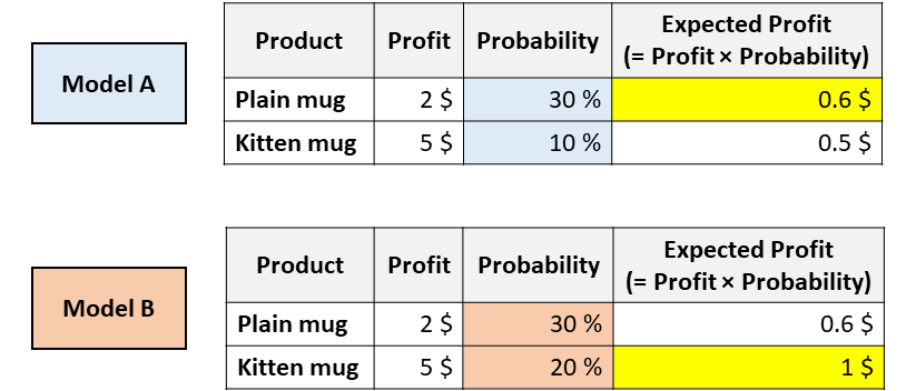
Какую кружку вы бы посоветовали этому пользователю?

Обе модели согласны с тем, что пользователь с большей вероятностью купит обычную кружку (так, модель A и модель B имеют одинаковую площадь под ROC, поскольку этот показатель только оценивает сортировку).

Но, согласно модели А, вы максимизируете ожидаемую прибыль, порекомендовав простую кружку. В то время как согласно модели B ожидаемая прибыль максимизируется кружкой для котенка.

В приложениях, подобных этому, очень важно выяснить, какая модель может лучше оценить вероятности.

В этой статье мы увидим, как измерить калибровку вероятности (как визуально, так и численно) и как «исправить» существующую модель, чтобы получить лучшие вероятности.

Что не так с «pred_proba»

Все самые популярные библиотеки машинного обучения в Python имеют метод под названием «pred_proba»: Scikit-learn (например, LogisticRegression, SVC, RandomForest,…), XGBoost, LightGBM, CatBoost, Keras…

Но, несмотря на свое название, pred_proba не совсем предсказывает вероятности. Фактически, разные исследования (особенно это и это) показали, что самые популярные прогностические модели не откалиброваны.

Тот факт, что число находится между нулем и единицей, недостаточно для того, чтобы назвать это вероятностью!

Но тогда когда мы можем сказать, что число на самом деле представляет собой вероятность?

Представьте, что вы обучили прогностическую модель предсказывать, разовьется ли у пациента рак. Теперь предположим, что для данного пациента модель предсказывает 5% вероятность. В принципе, мы должны наблюдать за одним и тем же пациентом в нескольких параллельных вселенных и смотреть, действительно ли он заболевает раком в 5% случаев.

Поскольку мы не можем идти по этой дороге, лучший пример — взять всех пациентов с вероятностью около 5% и подсчитать, у скольких из них развился рак. Если наблюдаемый процент фактически близок к 5%, мы говорим, что вероятности, предоставляемые моделью, «откалиброваны».

Когда предсказанные вероятности отражают реальные лежащие в основе вероятности, они называются «откалиброванными».

Но как проверить, откалибрована ли ваша модель?

Калибровочная кривая

Самый простой способ оценить калибровку вашей модели — это построить график под названием «калибровочная кривая» (также известная как «диаграмма надежности»).

Идея состоит в том, чтобы разделить наблюдения на интервалы вероятности. Таким образом, наблюдения, которые принадлежат одному интервалу, имеют одинаковую вероятность. В этот момент для каждого интервала калибровочная кривая сравнивает прогнозируемое среднее (т.е. среднее значение прогнозируемой вероятности) с теоретическим средним (т.е. средним значением наблюдаемой целевой переменной).

Scikit-learn выполняет всю эту работу за вас с помощью функции «Calibration_curve»:

from sklearn.calibration import calibration_curve
y_means, proba_means = calibration_curve(y, proba, n_bins, strategy)

Вам нужно только выбрать количество ящиков и (необязательно) стратегию объединения между:

• «Uniform», интервал 0–1 разделен на n_bins одинаковой ширины;
• «Квантиль», края интервала определяются таким образом, чтобы в каждом интервале было одинаковое количество наблюдений.

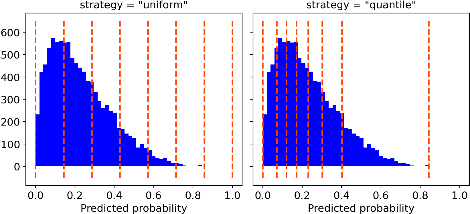
Для построения графиков я лично предпочитаю «квантильный» подход. Фактически, «равномерное» разбиение на интервалы может вводить в заблуждение, потому что некоторые интервалы могут содержать очень мало наблюдений.

Функция Numpy возвращает два массива, содержащих для каждой ячейки среднюю вероятность и среднее значение целевой переменной. Поэтому все, что нам нужно сделать, это построить их:

import matplotlib.pyplot as plt
plt.plot([0, 1], [0, 1], linestyle = '--', label = 'Perfect calibration')
plt.plot(proba_means, y_means)

Предположим, что ваша модель имеет хорошую точность, калибровочная кривая будет монотонно увеличиваться. Но это не значит, что модель хорошо откалибрована. Действительно, ваша модель хорошо откалибрована только в том случае, если калибровочная кривая очень близка к биссектрисе (т. Е. Пунктирной серой линии), поскольку это будет означать, что прогнозируемая вероятность в среднем близка к теоретической.

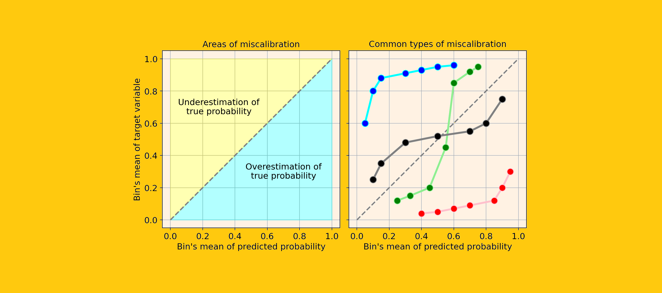
Давайте посмотрим на несколько примеров распространенных типов калибровочных кривых, указывающих на неправильную калибровку вашей модели:

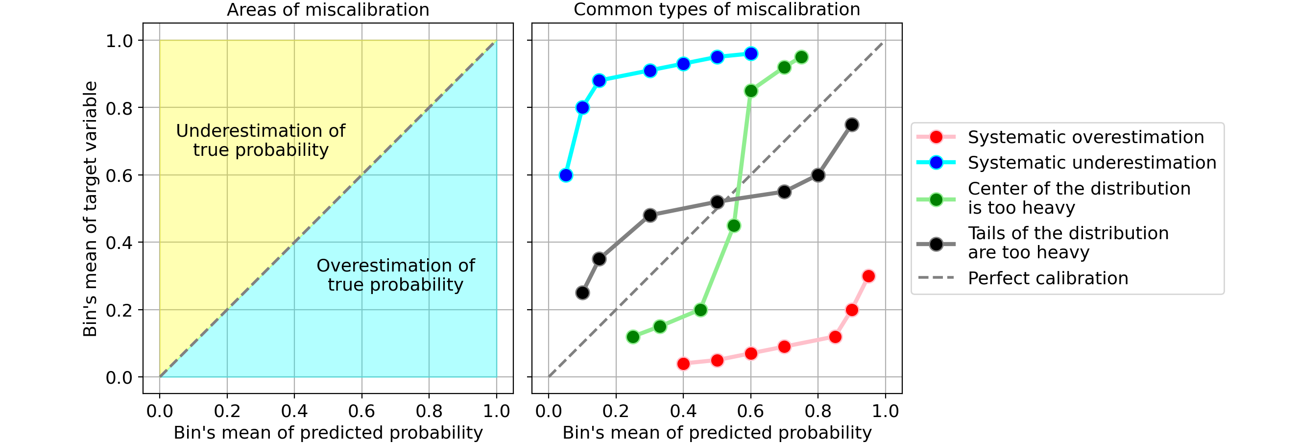
Наиболее распространенные типы ошибок калибровки:

• Систематическое завышение. По сравнению с истинным распределением, распределение предсказанных вероятностей сдвинуто вправо. Это обычное дело, когда вы обучаете модель на несбалансированном наборе данных с очень небольшим количеством положительных результатов.
• Систематическая недооценка. По сравнению с истинным распределением, распределение предсказанных вероятностей сдвинуто влево.
• Центр распределения слишком тяжелый. Это происходит, когда алгоритмы, такие как машины опорных векторов и деревья с усилением, имеют тенденцию отодвигать предсказанные вероятности от 0 и 1 (цитата из Предсказание хороших вероятностей с помощью контролируемого обучения).
• Слишком тяжелые хвосты раздачи. Например, Другие методы, такие как наивный байесовский метод, имеют противоположную предвзятость и склонны приближать прогнозы к 0 и 1 (цитата из Предсказание хороших вероятностей с помощью обучения с учителем).

Как исправить ошибку калибровки (в Python)

Предположим, вы обучили классификатор, который дает точные, но не откалиброванные вероятности. Идея калибровки вероятности состоит в том, чтобы построить вторую модель (называемую калибратором), которая может «скорректировать» их до реальных вероятностей.

Обратите внимание, что калибровку нельзя проводить на тех же данных, которые использовались для обучения первого классификатора.

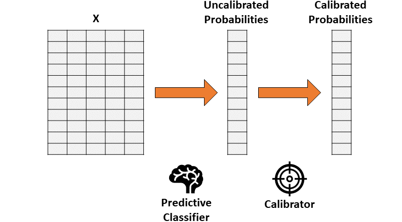
Следовательно, калибровка состоит в функции, которая преобразует одномерный вектор (некалиброванных вероятностей) в другой одномерный вектор (калиброванных вероятностей).

В качестве калибраторов в основном используются два метода:

• Изотоническая регрессия. Непараметрический алгоритм, который подгоняет неубывающую строку произвольной формы к данным. Тот факт, что строка не убывает, является фундаментальным, потому что соблюдается исходная сортировка.
• Логистическая регрессия.

Давайте посмотрим, как на практике использовать калибраторы в Python с помощью набора данных игрушек:

from sklearn.datasets import make_classification
X, y = make_classification(
    n_samples = 15000, 
    n_features = 50, 
    n_informative = 30, 
    n_redundant = 20,
    weights = [.9, .1],
    random_state = 0
)
X_train, X_valid, X_test = X[:5000], X[5000:10000], X[10000:]
y_train, y_valid, y_test = y[:5000], y[5000:10000], y[10000:]

Прежде всего, нам нужно будет подогнать классификатор. Давайте использовать случайный лес (но подойдет любая модель, в которой есть метод «pred_proba»).

from sklearn.ensemble import RandomForestClassifier
forest = RandomForestClassifier().fit(X_train, y_train)
proba_valid = forest.predict_proba(X_valid)[:, 1]

Затем мы будем использовать выходные данные классификатора (для данных проверки), чтобы соответствовать калибратору и, наконец, для прогнозирования вероятностей на тестовых данных.

• Изотоническая регрессия:

from sklearn.isotonic import IsotonicRegression
iso_reg = IsotonicRegression(y_min = 0, y_max = 1, out_of_bounds = 'clip').fit(proba_valid, y_valid)
proba_test_forest_isoreg = iso_reg.predict(forest.predict_proba(X_test)[:, 1])

• Логистическая регрессия:

from sklearn.linear_model import LogisticRegression
log_reg = LogisticRegression().fit(proba_valid.reshape(-1, 1), y_valid)
proba_test_forest_logreg = log_reg.predict_proba(forest.predict_proba(X_test)[:, 1].reshape(-1, 1))[:, 1]

На данный момент у нас есть три варианта прогнозирования вероятностей:

1. равнина случайный лес,
2. случайный лес + изотоническая регрессия,
3. случайный лес + логистическая регрессия.

Но как определить, какой из них наиболее откалиброван?

Количественная оценка ошибки калибровки

Сюжеты нравятся всем. Но помимо калибровочного графика нам нужен количественный способ измерения (ошибочной) калибровки. Наиболее часто используемый показатель называется Ожидаемая ошибка калибровки. Он отвечает на вопрос:

Насколько далеко в среднем наша предсказанная вероятность от истинной вероятности?

Возьмем, к примеру, один классификатор:

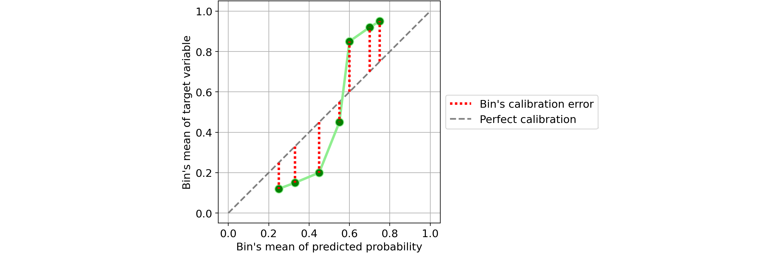
Определить ошибку калибровки отдельной ячейки очень просто: это абсолютная разница между средним значением предсказанных вероятностей и долей положительных результатов в одной ячейке.

Если задуматься, это довольно интуитивно понятно. Возьмем один бункер и предположим, что среднее значение его прогнозируемой вероятности составляет 25%. Таким образом, мы ожидаем, что доля положительных результатов в этом бине примерно равна 25%. Чем дальше это значение от 25%, тем хуже калибровка этого бина.

Таким образом, Ожидаемая ошибка калибровки (ECE) — это средневзвешенное значение ошибок калибровки отдельных интервалов, где каждый интервал весит пропорционально количеству содержащихся в нем наблюдений:

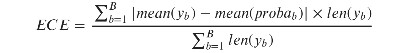
где b обозначает корзину, а B — количество корзин. Обратите внимание, что знаменатель — это просто общее количество образцов.

Но эта формула оставляет нам проблему определения количества ящиков. Чтобы найти максимально нейтральный показатель, я предлагаю установить количество ящиков в соответствии с правилом Фридмана-Диакониса (которое является статистическим правилом, предназначенным для нахождения количество интервалов, которое делает гистограмму максимально приближенной к теоретическому распределению вероятностей).

Использовать правило Фридмана-Диакониса в Python чрезвычайно просто, поскольку оно уже реализовано в функции гистограммы numpy (достаточно передать строку «fd» в параметр «bins»).

Вот реализация Python ожидаемой ошибки калибровки, в которой по умолчанию используется правило Фридмана-Диакониса:

def expected_calibration_error(y, proba, bins = 'fd'):
  import numpy as np
  bin_count, bin_edges = np.histogram(proba, bins = bins)
  n_bins = len(bin_count)
  bin_edges[0] -= 1e-8 # because left edge is not included
  bin_id = np.digitize(proba, bin_edges, right = True) - 1
  bin_ysum = np.bincount(bin_id, weights = y, minlength = n_bins)
  bin_probasum = np.bincount(bin_id, weights = proba, minlength = n_bins)
  bin_ymean = np.divide(bin_ysum, bin_count, out = np.zeros(n_bins), where = bin_count > 0)
  bin_probamean = np.divide(bin_probasum, bin_count, out = np.zeros(n_bins), where = bin_count > 0)
  ece = np.abs((bin_probamean - bin_ymean) * bin_count).sum() / len(proba)
  return ece

Теперь, когда у нас есть метрика для калибровки, давайте сравним калибровку трех моделей, которые мы получили выше (на тестовом наборе):

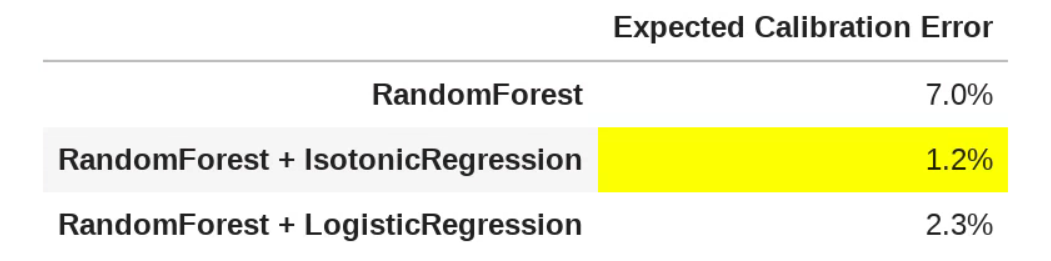
В этом случае изотоническая регрессия дала лучший результат с точки зрения калибровки, в среднем составляя всего 1,2% от истинной вероятности. Это огромное улучшение, если учесть, что ECE равнинного случайного леса составлял 7%.

Ссылка

Вот несколько интересных статей (на которых основана эта статья), которые я рекомендую, если вы хотите углубить тему калибровки вероятностей:

• Прогнозирование хороших вероятностей с помощью контролируемого обучения (2005) Каруаны и Никулеску-Мизил.
• О калибровке современных нейронных сетей (2017) Guo et al.
• Получение хорошо откалиброванных вероятностей с использованием байесовского биннинга (2015) Naeini et al.

Спасибо за чтение! Надеюсь, этот пост был вам полезен.

Я ценю отзывы и конструктивную критику. Если вы хотите поговорить об этой статье или о других связанных темах, вы можете написать мне на мой контакт в Linkedin.