9The lognormal distribution fares slightly better than the normal distribution by having more probability in the tails — that is, having higher values of integrals ∫baP(x)dx for a – b ranges covering larger x values.
From: Philosophy of Complex Systems, 2011
Advanced Math and Statistics
Robert Kissell, Jim Poserina, in Optimal Sports Math, Statistics, and Fantasy, 2017
Log-Normal Distribution
A log-normal distribution is a continuous distribution of random variable y whose natural logarithm is normally distributed. For example, if random variable y=exp{y} has log-normal distribution then x=log(y) has normal distribution. Log-normal distributions are most often used in finance to model stock prices, index values, asset returns, as well as exchange rates, derivatives, etc.
Log-Normal Distribution Statistics1
| Notation | lnN(μ,σ2) |
| −∞<μ<∞ | |
| Parameter | σ2>0 |
| Distribution | x>0 |
| 12πσxexp{−(ln(x)−μ)22σ2} | |
| Cdf | 12[1+erf(ln(x−μ)σ)] |
| Mean | e(μ+12σ2) |
| Variance | (eσ2−1)e2μ+σ2 |
| Skewness | (eσ2+2)(eσ2−1) |
| Kurtosis | e4σ2+2e3σ2+3e2σ2−6 |
where erf is the Gaussian error function.
Log-Normal Distribution Graph

Read full chapter
URL:
https://www.sciencedirect.com/science/article/pii/B9780128051634000049
Cumulative exposure model
Debasis Kundu, Ayon Ganguly, in Analysis of Step-Stress Models, 2017
2.6.2 Log-normal distribution
The log-normal distribution has been used quite extensively in analyzing lifetime data. If X has a normal distribution then eX has a log-normal distribution. Therefore, a log-normal distribution with the scale parameter 0<λ<∞ and the shape parameter σ > 0 has the following CDF:
F(t;λ,σ)=0ift<0Φln(t)−ln(λ)σift≥0.
The corresponding PDF and hazard function become
f(t;λ,σ)=0ift<01σtϕln(t)−ln(λ)σift≥0,
and
h(t;λ,σ)=ϕln(t)−ln(λ)σσtΦ−ln(t)+ln(λ)σ;t>0,
respectively. The PDF and the hazard function of a log-normal distribution are always unimodal functions. The PDF of a log-normal distribution is very similar to the PDFs of gamma, Weibull or generalized exponential distributions when the shape parameters of gamma, Weibull and generalized exponential distributions are greater than one. It has been shown by Kundu and Manglick [85, 86] and Kundu et al. [87] that it is very difficult to discriminate between log-normal and gamma, log-normal and Weibull and log-normal and generalized exponential distributions. For different properties of a log-normal distribution and for its various applications, one is referred to Johnson et al. [59].
Alhadeed [88] considered in his PhD thesis the analysis of the log-normal step-stress model, see also Alhadeed and Yang [34], when the complete data are available. Balakrishnan et al. [55] considered the same problem when the data are Type-I censored. It is assumed that the lifetime distribution of the experimental units at the two different stress levels follow log-normal distributions with different scale parameters, λ1 and λ2, but the same shape parameter σ. Based on the CEM assumption, the CDF of the lifetime of an experimental unit from a simple step-stress model can be written as
(2.40)F(t)=0ift<0Φln(t)−ln(λ1)σif0≤t<τ1Φlnt+τ1λ2λ1−τ1−ln(λ2)σifτ1≤t<∞.
Hence, the PDF corresponding to Eq. (2.40) becomes
(2.41)f(t)=0ift<01σtϕln(t)−ln(λ1)σif0≤t<τ11σt+λ2λ1τ1−τ1ϕlnt+τ1λ2λ1−τ1−ln(λ2)σifτ1≤t<∞.
In this case it is more convenient to work with the log-transformation of the data than the original data. Now if a random variable T has the PDF (2.41), then Y=ln(T) has the PDF
fY(y)=0ift<01σϕy−μ1σif0<t<lnτ1eyσey+eμ2−μ1τ1−τ1ϕlney+τ1eμ2−μ1−τ1−μ2σiflnτ1≤y<∞.
Here μ1=lnλ1 and μ2=lnλ2. Therefore, if we denote the log of the observed lifetimes as yi:n=ln(ti:n) for i = 1, …, n, then the log-likelihood function based on the complete observations {y1:n, …, yn:n} is
(2.42)l(μ1,μ2,σ)=−n2ln(π)−nlnσ−12∑i=1n1yi:n−μ1σ2−∑i=n1+1nln(eyi:n+τ1eμ2−μ1−τ1)−12∑i=n1+1nln(eyi:n+τ1eμ2−μ1−τ1)−μ2σ2.
Here it is assumed that 1 ≤ n1 ≤ n − 1 and n ≥ 3; otherwise it is known that the MLEs of σ, μ1, and μ2 do not exist. Therefore, the conditional MLEs of the unknown parameters conditioning on 1 ≤ N1 ≤ n − 1 can be obtained by maximizing Eq. (2.42) with respect to the unknown parameters. In this case the normal equations become
(2.43)l.μ1=∑i=n1+1nτ1eμ2−μ1eyi:n+τ1eμ2−μ1−τ1+1σ2∑i=1n1(yi:n−μ1)+1σ2∑i=n1+1n(ln(eyi:n+τ1eμ2−μ1−τ1)−μ2)τ1eμ2−μ1eyi:n+τ1eμ2−μ1=0,
(2.44)l.μ2=−1σ2∑i=n1+1n(ln(eyi:n+τ1eμ2−μ1−τ1)−μ2)τ1eμ2−μ1eyi:n+τ1eμ2−μ1−1−∑i=n1+1nτ1eμ2−μ1eyi:n+τ1eμ2−μ1−τ1=0,
(2.45)l.σ=−nσ+1σ3∑i=1n1(yi:n−μ1)2+1σ3∑i=n1+1n(ln(eyi:n+τ1eμ2−μ1−τ1)−μ2)2=0.
Clearly, Eqs. (2.43)–(2.45) cannot be solved explicitly. One needs to use the Newton-Raphson type iterative algorithm to solve Eqs. (2.43)–(2.45) numerically. Some initial guesses of the parameters are needed to start the iteration. If μ1 and μ2 are known, the MLE of σ2 can be obtained from Eq. (2.45) as
(2.46)σ^2(μ1,μ2)=1n∑i=1n1(yi:n−μ1)2+∑i=n1+1n(ln(eyi:n+τ1eμ2−μ1−τ1)−μ2)2.
We can obtain the profile log-likelihood function of μ1 and μ2 by using Eq. (2.46) in Eq. (2.42). The profile log-likelihood function of μ1 and μ2 without the additive constants can be written as
(2.47)p(μ1,μ2)=−n2ln∑i=1n1(yi:n−μ1)2+∑i=n1+1n(ln(eyi:n+τ1eμ2−μ1−τ1)−μ2)2−∑i=n1+1nln(eyi:n+τ1eμ2−μ1−τ1).
A contour plot of p(μ1, μ2) as in Eq. (2.47) may provide good starting values of μ1 and μ2. Once we obtain the starting values of μ1 and μ2, the starting value of σ can be easily obtained from Eq. (2.46). Although we have presented the results here for the complete sample, similar results can be developed for different censoring schemes. Balakrishnan et al. [55] performed an extensive simulation study to compare the performances of different confidence intervals. It is observed that the biased corrected bootstrap method works very well in this case. Most of the results have been extended by Lin and Chou [56] for the multiple step-stress model.
Read full chapter
URL:
https://www.sciencedirect.com/science/article/pii/B9780128097137000028
The particle size distribution
Miroslaw Jonasz, Georges R. Fournier, in Light Scattering by Particles in Water, 2007
5.8.5.6 The log-normal function
Like the power-law distribution discussed in section 5.8.5.3, the log-normal probability distribution has applications in diverse areas, ranging from business (Shimizu and Crow 1988) to oceanography (Campbell 1995). Limpert et al. 2001 review applications of the log-normal distribution in various sciences. The log-normal distribution is generally the result of a process, which can be mathematically characterized by a product of many random variables, for example the process of fragmentation. Indeed, a fragmentation process with the probability of fragmentation independent of the particle size leads to the log-normal function (Shimizu and Crow 1988, Middleton 1970) as originally found by Kolmogorov in 1941 (cited by Tenchov and Yanev 1986). If the probability of fragmentation is proportional to the particle size, the Weibull distribution (section 5.8.5.10) results. However, the difference between a log-normal distribution and a Weibull distribution may be made quite small by the appropriate selection of the distribution parameters (Tenchov and Yanev 1986). Thus, it may be difficult to discern at the measurement precision characteristic of the particle size analysis techniques applicable to aquatic particles. Aitchinson and Brown (1957, Section 10.2) summarize applications of the log-normal distribution in the approximation of the PSD. Crow (1988) discusses applications of the log-normal distribution to model the size distribution of atmospheric particles. Heintzenberg (1994) discusses the properties of the log-normal distribution as applicable to PSD approximations and calculations.
The use of log-normal distributions for approximating the PSD has important advantages:
- (1)
-
there is no need to “break” the power-law approximation to reflect changes in the log-log slope of the size distribution;
- (2)
-
the log-normal approximation assumes finite values for all particle diameters, except in the limit B2 > 0, when the log-normal function becomes a power-law function;
- (3)
-
mass and area distributions resulting from the log-normal distribution are also log-normal (Kerker 1969);
- (4)
-
the power-law function is a limiting case of the log-normal function, so it is naturally included as an approximation of the size distribution.
We should also mention certain pitfalls of choosing the log-normal distribution after Halley and Inchausti (2002), who cite comments by Mandelbrot (1997) (incidentally these problems also relate to other “long-tailed” distributions):
- (1)
-
extreme sensitivity of all moments of the distribution to even small departures from log-normality, which makes the calculation of moments from the parameters of a fitted log-normal distribution unreliable
- (2)
-
slow convergence of the approximate values of the moments to their asymptotic value. This feature is due to an extremely “long tail” of the log-normal distribution at the large-size end of the particle size scale. We have experienced this problem ourselves (Jonasz and Fournier 1996) when trying to evaluate correlations between the total particle surface and volume and the peak diameter of the distribution as fitted to several hundred size distributions of marine particles.
The log-normal size distribution of the zero-th order can be expressed as follows (e.g., Ross 1978, Casperson 1977):
(5.169)n(D)=nmaxexp[−(lnD−lnDpeak)22σ2]
where nmax is expressed as follows:
(5.170)nmax=Ntot2πσDpeakexpσ22
Ntot is the total number of particles [equal to unity in the case of n(D) being the probability distribution], Dpeak is the particle diameter corresponding to the peak of the size distribution, and σ is the standard deviation of lnD, i.e., the geometric standard deviation of D.
The width parameter, σ, is related to the ratio of the maximum and minimum diameters, Dmax and Dmin, of the full-width-at-half-maximum of the log-normal n(D) through the following equation (Jonasz and Fournier 1996):
(5.171)DmaxDmin=exp(2fσ)
where
(5.172)f=2ln2Dmin=Dpeakexp(−fσ)Dmin=Dpeakexp(fσ)
In contrast to the power-law distribution, the log-normal size distribution yields a finite total number of particles, Ntot, total particle cross-sectional area, Atot, and volume, Vtot (Heintzenberg 1994):
(5.173)Atot=π[12Dpeakexp(2σ2)]2Ntot×exp{−12σ2[(lnDmaxexp(2σ2))−lnDmax]2}
and
(5.174)Vtot=43π[12Dpeakexp(3σ2)]3Ntot×exp{−12σ2[(lnDmaxexp(3σ2))−lnDmax]2}
Equations (5.173) and (5.174) apply to the –1-th order generalized log-normalparticle size distribution (see, e.g., Casperson 1977), not to the zero-th ordermostly discussed in this section.
Note that successful applications of these formulas, as also pointed out by Heintzenberg (1994), require that the parameters of the log-normal distribution be evaluated for a particle size range that contributes significantly to the total projected area and volume.
The log-normal function was postulated to approximate the size distribution of marine particles in samples of seawater from several GEOSECS stations in the Atlantic and Pacific, at depths ranging from 286 to 5474 m (Lambert et al. 1981). The particles were collected on 0.4 μm Nuclepore filters and analyzed with a scanning electron microscope. Portions of the filters were coated with carbon and examined using a scanning electron microscope equipped with an X-ray elemental analysis accessory, which enabled the determination of species-specific PSDs. A total of between 100 and 500 particles were analyzed for each sample in a diameter range of 0.2 to 10 μm. The diameter of a particle is taken to be the diameter of a circle with an area equal to that of the particle. The peak diameter was between 1 and 2.5 μm, and the width parameter σ of the size distribution was found to be in a range of 0.5 to 0.7. The quality of the log-normal approximation could in some cases be significantly improved by eliminating the extreme data points in the tails of the distribution. This might be due to the presence in the size distribution of other modes, due to particle populations marginally overlapping in size with the main particle size range.
The log-normal function was also found to approximate well the size distributions of non-spherical clay particles (Jonasz 1987b) measured using a Coulter counter, model ZBI with a 100 μm aperture, and using an HIAC particle counter, model 320 with a CMH-150 particle size sensor.
The cell size distributions reported in the literature frequently appear to be log-normal at visual inspection (see Table A.5 for sources of the relevant PSD data). Interestingly, mathematical models of cell growth and evolution of isolated cell populations do not lead to a log-normal distribution of cell sizes (e.g., Tyson and Hannsgen 1985). However, the agreement between the models and the experimental data is questionable. In fact, Tyson and Hannsgen note that cell size distributions with log-normal size distribution have been reported (ibid. Scherbaum and Rasch 1957, Collins and Richmond 1962). Analysis of the biomass spectrum in aquatic ecosystems composed of organism groups linked via a prey–predator relationship led to the log-normal function as a natural descriptor of the contribution of an organism to the total ecosystem biomas spectrum (Thiebaux and Dickie 1993, Boudreau et al. 1991). The derivation of the log-normal form of the size distributions of the individual organism groups was based on the fact that the production, P (w), is proportional to a power, b, of the body mass, W (allometric relationship):
(5.175)P(W)=aWb
The observation of (1) a persistent curvature of the size distribution of marine particles, when plotted in a log-log scale, (2) the multimodal appearance of many such size distributions, as well as (3) previous suggestions in the literature that complex size distributions of geological material can be well modeled by a sum of log-normal functions (van Andel 1973) led us to develop an automated algorithm of the decomposition of a marine PSD into a sum of log-normal components (Jonasz and Fournier 1999, 1996). In that work, we postulated that the size distribution of marine particles is essentially a linear combination of a cascade of log-normal components, according to the following equation:
(5.176)n(D)=∑1kmaxnk(D)
where index k numbers the log-normal components nk(D). Each of these components is approximated with a zero-th order log-normal distribution function:
(5.177)nk(D)=nmax,kexp[−(lnD−lnDpeak,k)22σk2]
where nmax, k is the maximum value of the component, Dpeak,k [μm] is the peak diameter, and σk is the width parameter. By taking the logarithm of both sides of (5.177) and performing simple algebraic transformations, one obtains (we omit the component index for simplicity):
(5.178)logn(D)=B0+B1logD+B2(logD)2
where:
(5.179)B0=lognmax−(logDpeak)2ln102σ2B1=logDpeakln10σ2B2=−ln102σ2
Note that (5.178) reduces to a power law when B2 vanishes. Equations (5.179) can be solved for nmax, Dpeak, and σ to yield:
(5.180)lognmax=B0−B124B2logDpeak=−B12Bσ2=−ln102B2
We consider only those functions defined by (5.177) which fulfill the condition of B2 < 0. This ensures that the extremum of the function is a maximum. According to the assumption about the size distribution being a cascade of log-normal components, each log-normal component dominates in a particular size interval. Thus, if that size interval is somehow identified, one could determine the parameters of the respective log-normal component, for example, by using the least-squares fitting procedure for the log-log transformed original data.
In the algorithm of Jonasz and Fournier (1996) for fitting a sum of log-normal functions to PSD data, the size interval dominated by a particular log-normal function is identified by repeatedly scanning the size distribution with a window whose width is systematically varied. During each scan set with a fixed window width, the log-normal function is fitted to the data from within the window. Since the number of data points in a size distribution is usually quite moderate, the quality of the log-normal fit for all realistic window widths and locations can be assessed. Once a log-normal component is found, it is subtracted from the PSD data, and the modified data serve as the input for the next round of scans with this window width. If the PSD value (data point) from which a component value at that particle size has been subtracted falls below a preset limit, that data point is removed from the set. Thus, normally the number of data points decreases during this procedure which is terminated if there is no sufficient data left or, less likely, if no components have been found. For each of the next set of scans, the window width is incremented by unity, until the maximum allowed window width. Each set of scans may result in a set of log-normal components which approximate the original data with a specific accuracy. The algorithm is completed by selecting a set of log-normal fits based on either the minimum of the approximation error or other criterion set by the user, for example, the approximation error and the number of components.
Important comments are in order here. First, although the PSD may be better approximated with several, “interpretable” components, the extent of this interpretability is limited by the number of degrees of freedom of the data set, because each log-normal component reduces the number of degrees of freedom by 3. Second, each new component increases the number of parameters required for the description of the data set. From the purely numerical perspective, this seems to be counterproductive—we noted earlier that one goal of the approximation is to reduce the number of parameters. Indeed, given a sufficiently large number of components one simply exchanges the original data (the primary set of parameters) by an equally numerous set of the fit parameters. However, once the “interpretability” aspect is acknowledged, the advantage of that exchange should become clear, as there is usually little interpretability in the original data set. We also discuss this aspect of the PSD analysis later in this section.
Sample results are shown in Figure 5.34 and Figure 5.35. Log-normal components identified by the algorithm just described range in shape from the power-law-like function to Gaussian-normal-like function. Note that the failure to account for the instrumental error (see section 5.7.1.6) in evaluating the γ2 results in the γ2 value in excess of 200 per degree of freedom (!) in the case of data shown in Figure 5.35. that include very high particle count values.

Figure 5.34. A log-normal approximation of the size distribution of Figure 5.31: log n (D) = 4.41 − 2.50 log D − 1.02 (log D)2 (γ2 per degree of freedom = 0.24). The fit parameters were obtained via the logarithmic transform. All weights were set to unity. The γ2 was calculated by assuming only the counting error.

Figure 5.35. A multi-component log-normal approximation (thick black curve) of a PSD measured in the Northwest Atlantic waters (•, unpublished data: courtesy of K. Kranck and T. Milligan, file KRAATL86.P08 in Jonasz 1992). The approximation coefficients from equation (5.178) : first component (thin solid curve) B01 = 4.05, B11 = −1.16, B21 = −2.12, second component (dashed curve) B02 = −17.04, B12 = 22.52, B22 = −7.75, third component (gray solid curve) B03 = 4.97, B13 = 7.04, B23 = 7.30, fourth component (gray dashed curve) B04 = −4.27, B14 = −9.60, B24 = −4.81. The first log-normal component removes the greatest amount of the approximation error. Each of the following components removes a progressively smaller amount of that error (χ2 per degree of freedom = 0. 021). The fit parameters were obtained via the logarithmic transform. All fitting weights were set to unity. The χ2 was calculated by assuming both the counting and instrumental errors.
The statistics of and correlations between the parameters of 853 log-normal components of the 412 PSDs determined using the Coulter technique by different researchers in different areas and seasons are shown in Table 5.10. The average values of coefficients B0, B1, and B2 represent a geometrically averaged component characteristics, i.e., navg(D) such that navg(D) = [n1(D) n2(D) … nm(D)]1/m. The average values of nmax, Dpeak, and σ do not have simple meanings and are given here for the sake of completeness only. The two sets of averages do not yield the same function of the diameter, D, because they are related via non-linear functions (5.179) and (5.180). The average error of approximation of the size distribution with the sum of log-normal components was 0.057±0.030. The number of components per size distribution varied from 1 to 6, with an average of 2.18 ± 1.22. The value of 1 standard deviation (SD) is shown following the ± sign.
Table 5.10. Correlations, expressed using r2, between the parameters of log-normal components of marine particle size distributions measured with a Coulter counter (Jonasz and Fournier 1996—412 size distributions measured by various authors in various seasons and areas of the world ocean).
| Parameter | ln nmax | ln Dpeak | σ |
|---|---|---|---|
| ln nmax | 1.000 | 0.873 | 0.478 |
| ln Dpeak | 0.873 | 1.000 | 0.760 |
| σ | 0.478 | 0.760 | 1.000 |
| Parameter | B0 | B1 | B2 |
| B0 | 1.000 | 0.963 | 0.840 |
| B1 | 0.963 | 1.000 | 0.942 |
| B2 | 0.840 | 0.942 | 1.000 |
The correlations between the coefficients, B0,B1, and B2 are greater than those between the parameters nmax, D ak, and a because of the smoothing effect of the logarithmic transform.
Significant correlations exist between the Dpeak and nmax, as well as between Dpeak and the width parameter, σ, of the component, as can be seen in Figure 5.36 and Figure 5.37. The equations of the approximating lines (see also the correlation coefficients in Table 5.10) shown in these two figures are respectively:

Figure 5.36. Relationship between σ and Dpeak for 853 log-normal components of 412 particle size distributions (Jonasz and Fournier 1996) measured in various waters and seasons by several researchers (as compiled by Jonasz 1992). Approximation line equation: σ = (0.626 ± 0.186) – (0.111 ± 0.002) ln Dpeak, with 1 SD shown following each ± sign (r2 = 0.760).

Figure 5.37. Relationship between nmax and Dpeak for 853 log-normal components of 412 particle size distributions (Jonasz and Fournier 1996) measured in various waters and seasons by several researchers (as compiled by Jonasz 1992). The range of nmax is limited to keep the number of decades on the nmax-axis manageable. The data points not shown conform to the general trend. Approximation line equation: ln nmax = (8.070 ± 2.799) – (2.446 ±0.032) lnDpeak, with 1 SD shown following each ± sign (r2 = 0.873).
(5.181)lnnmax=(8.070±2.799)−(2.446±0.032)lnDpeak
and
(5.182)σ=(0.626±0.186)−(0.111±0.002)lnDpeak
where the value of 1 SD of the respective parameter is shown following each ± sign.
The log-normal components, which range in shape from the power-law-like function to Gaussian-normal-like function, may be interpreted as the size distributions of the various classes of marine particles, for example, populations of various phytoplankton species. Indeed, Jonasz and Fournier (1996) found two “standard” components (Figure 5.38 and Table 5.11) in 412 size distributions measured in various seasons and regions of the world ocean by different researchers. Bradtke (2004) who used the algorithm just described to analyze 970 PSDs measured with a Coulter counter in the coastal waters of the Baltic Sea (Gdansk Bay) also noted the existence of several “standard” components and linked other transitional components to the occurrences of phytoplankton species.

Figure 5.38. “Standard” components (Table 5.11) of the marine particle size distribution identified by Jonasz and Fournier (1996), who analyzed 412 particle size distributions measured in various seasons and regions of the world ocean by different researchers (as compiled by Jonasz 1992): first component (solid black curve) B01 = 4.038, B11 = −0.9511, B21 = −2.542, second component (dashed curve) B02 = −8.447, B12 = −7.55, B22 = −8.595, compared with the size distribution from Figure 5.35 (symbols) and its retrieved components (gray solid lines).
Table 5.11. Parameters of two “standard” components of the marine size particle distribution (Jonasz and Fournier 1996).
| Parameter | Component 1 | Component 2 |
|---|---|---|
| nmax [μm−1 cm−1 | 13400 | 3.28 |
| Dpeak[μm] | 0.65 | 10.5 |
| σ | 0.673 | 0.366 |
| B0 | 4.038 | -8.447 |
| B1 | -0.9511 | 17.55 |
| B2 | -2.542 | -8.595 |
Although “standard” components of the marine size distribution can be generated by other techniques, for example, by the method of characteristic vectors (see section 5.8.5.11), these components lack the physical and biological interpretation possible for the log-normal components. The existence of “standard” components as identified by Bradtke (2004) as well as Jonasz and Fournier (1996) with this algorithm is remarkable, as the decomposition algorithm approaches the task from a purely numerical perspective. It would have certainly been desirable to enhance it so that such “standard” log-normal components attributable to various particle species would be searched for rather than arbitrary log-normal functions whose sum happens to minimize the approximation error of the PSD.
This approach would be particularly attractive from the biological point of view, given the use of log-normal functions to represent ecosystems in natural waters (Thiebaux and Dickie 1993, Boudreau et al. 1991). However, intraspecies variability of the PSDs “characteristic” for a particle species (see examples in section 5.8.4.4.) may make such a decomposition difficult especially when the differences between the approximation errors of a size distribution with various component sets are relatively small.
Jonasz and Fournier (1996) found that only about 5% of the components of the marine size distribution could be well approximated with a power law, which is represented with a straight line on a plot of log n (D) vs. log D. Interestingly, this conclusion does not rule out the first-order representation of the PSD of marine particles by a power-law function in a large range of particle diameter. Such a function would simply be an envelope of the sum of log-normal components.
Read full chapter
URL:
https://www.sciencedirect.com/science/article/pii/B9780123887511500053
Other related models
Debasis Kundu, Ayon Ganguly, in Analysis of Step-Stress Models, 2017
Log-normal distribution
The classical inferential issues of the TRVM under the assumption that T has a log-normal distribution with the PDF
fT(t)=1σt2πe−12lnt−μσ21(0,∞)(t),
where μ∈R and σ > 0, was addressed by Bai et al. [115]. The authors also assumed that the data are Type-I censored. Under the log-normal distribution, the PDF of T~ is given by
fT~(t)=1σt2πe−12lnt−μσ2if0<t≤τ1βστ1+β(t−τ1)2πe−12ln(τ1+β(t−τ1))−μσ2ift>τ10otherwise.
Given a Type-I censored data t1:n<⋯<tn1:n<τ1<tn1+1:n<⋯<tn1+n2:n<η, the log-likelihood function can be written as
l(μ,σ2,β)=−n1+n22lnσ2−∑i=n1+1n1+n2lnτ1+β(ti:n−τ1)−12σ2∑i=1n1lnti:n−μ2−12σ2∑i=n1+1n1+n2ln(τ1+β(ti:n−τ1))−μ2+(n−n1−n2)ln1−Φln(τ1+β(η−τ1))−μσ,
where Φ(⋅) is the CDF of the standard normal distribution. The MLEs of μ, σ2, and β can be found by maximizing the log-likelihood function with respect to the parameters. Note that in this case the MLEs of the unknown parameters do not exist in explicit form and one needs to use a numerical technique to maximize the log-likelihood function. The asymptotic variance of the MLEs and the confidence intervals of the unknown parameters can be obtained using the observed Fisher information matrix.
Read full chapter
URL:
https://www.sciencedirect.com/science/article/pii/B978012809713700003X
AFM and Development of (Bio)Fouling-Resistant Membranes
Nidal Hilal, … Huabing Yin, in Atomic Force Microscopy in Process Engineering, 2009
Pore Size and Pore Size Distribution
Pore size and PSD of each membrane were determined from AFM-determined topography. The lognormal distribution was chosen to represent the pore size data for each of the membranes. This was found to give a good fit to the PSD. All of these distributions were fitted to lognormal distributions given by frequencies (%f):
(5.1)%f=%fmaxexp[-12σ2ln(dpX0)2]
where dp is the measured pore size, σ the standard deviation of the measurements, %fmax the maximum frequency and χ0 the modal value of dp.
Mean pore sizes and PSDs of initial membranes determined from AFM images are shown in Table 5.3. This table shows that with a mean pore size of 0.535±0.082 μm, the PVDF membrane has slightly larger pores than the PES membrane (mean pore size 0.470±0.188 μm). PSDs are detailed in Figure 5.3, along with fits described by equation (5.1). The measured pore sizes are larger than the nominal pore size of 0.22 μm as specified by the manufacturers. The AFM data confirm that the pore sizes of studied membranes are of approximately the same size. The topographical images give a clear perception of a notable difference in the surface morphology of the membranes used for the modification. A quantification of the surface parameters (Table 5.3) provides an insight into morphological particularities of these membranes which influence both the membrane separating properties and the process of modification by graft copolymerisation.
Table 5.3. Parameters of Pore Size and PSD Obtained from AFM Images for Initial PES and PVDF Membranes.
| Pore size (μm) | PSD parameters | |||||
|---|---|---|---|---|---|---|
| Membrane | Mean | Minimum | Maximum | X0 (μm) | %fmax | σ |
| PES | 0.470±0.188 | 0.219 | 0.948 | 0.353±0.028 | 19.8±2.2 | 0.56±0.08 |
The two membranes under study have notably different PSDs. It can be noted here that PVDF has a narrower PSD with pore sizes from 0.336 to 0.68 μm compared with a PSD ranging from 0.219 to 0.948 μm in PES membranes. Moreover, these membranes significantly differ in surface roughness, with the PES membrane being smoother than the PVDF membrane. Regarding the AFM images, one might notice that the smoother surface allows for better contrast in pore observation, but more importantly the surface roughness is expected to have an influence on the graft copolymerisation.
The rate of membrane modification was higher in the case of PES membrane than PVDF membrane [19]. It is impossible to associate the difference only with the contribution of surface morphology. It is well known that polysulphone and PES are intrinsically photo-active, undergoing bond cleavage with UV irradiation to produce free radicals even without the use of photo-initiators. PVDF is less photo-reactive than PES and produces less surface free radicals than PES. However, higher density of free radicals at the surface of more photo-reactive PES membranes also results in a higher probability of termination of chain growth and formation of cross-linked structures. These processes restricting an increase in the DM are competitive with respect to the chain growth. Since competitive processes, which enhance and decrease the amount of grafted polymer, occur simultaneously in the case of the photo-reactive polymer, the influence of surface morphology on graft copolymerisation should not be discarded. For the relatively rough surfaces, such as PVDF membrane, the decrease in UV-irradiation effectiveness and steric hindrance for polymer growth in narrow valleys are possible effects that may decrease the modification to some degree.
Before detailed discussion of the quantitative characteristics of surface morphology, it is worth noting that the chosen lognormal pattern for PDS described by equation (5.1) gave a correlation coefficient of at least 0.95 for all fitted curves. The most probable pore sizes estimated from fitted curves were very close to the mean pore diameter calculated from corresponding sets of pore sizes for the initial and modified membranes (Tables 5.4 and 5.5).
Table 5.4. AFM Measurements of Pore Size and PSD of Initial and Modified PES Membranes with qDMAEMA.
| Mean pore | PSD parameters | |||
|---|---|---|---|---|
| DM (μg/cm2) | size (μm) | X0 (μm) | %fmax | σ |
| 0 | 0.470±0.188 | 0.353±0.028 | 19.8±2.2 | 0.56±0.08 |
| 202 | 0.337±0.098 | 0.278±0.010 | 41.4±4.4 | 0.32±0.04 |
| 367 | 0.293±0.072 | 0.281± 0.003 | 51.3±2.0 | 0.26±0.01 |
| 510 | 0.100±0.083 | 0.075±0.004 | 26.9±2.9 | 0.40±0.05 |
Table 5.5. AFM Measurements of Pore Size and PSD of Initial and Modified PVDF Membranes with qDMAEMA.
| Mean pore | PSD parameters | |||
|---|---|---|---|---|
| DM (μg/cm2) | size (μm) | X0 (μm) | %fmax | σ |
| 0 | 0.535±0.082 | 0.555±0.003 | 51.2±1.7 | 0.14±0.01 |
| 224 | 0.445±0.083 | 0.439±0.018 | 35.1±4.1 | 0.28±0.02 |
| 346 | 0.334±0.079 | 0.297±0.013 | 44.3±5.7 | 0.30±0.01 |
According to Figure 5.5(a), the initial PES membrane has a very wide PSD with a σ value of 0.56 μm. However, grafting of poly-qDMAEMA resulted in narrowing of the PSD and shifting the whole curve towards smaller pore sizes. As a result, mean pore size is gradually decreasing with the increase in the amount of poly-qDMAEMA grafted to the membrane surface. Significant improvement of the PSD was observed even for the modified PES membranes with the smallest DM (Table 5.4).

Figure 5.5. PSDs of initial (a) and modified with qDMAEMA (b)–(d) PES membranes; (b) DM = 202 μg cm−2, (c) DM = 367 μg cm−2 and (d) DM = 510 μg cm−2.
Narrowing of the PSD occurred mostly due to the disappearance of large pores (larger than 0.6 μm). Taking into consideration that substantial narrowing of large pores demands higher quantities of grafted polymer compared to smaller pores, it can be assumed that higher rates of polymer growth initiated at the walls of larger pores. As mentioned earlier, at the entrance of narrower pores, higher density of free radicals results in chain termination and consequently lower rate of polymer grafting. With time, when the PSD becomes more uniform, free radicals are eventually distributed across the membrane surface. This leads to a gradual decrease of all surface pores with PSD shifting to smaller sizes. With DM higher than 202 μm cm−2, slight fluctuation in the width of PSD (σ) was observed.
It can be seen from Table 5.5 that similar behaviour is observed regarding changes in the surface morphology of the PVDF membrane as for the PES membrane. However, the unmodified PVDF membrane has a more uniform PSD than the PES membrane. With a mean pore size approximately 0.54 μm, PSD of this membrane is characterised by a low value of σ, ∼0.14 μm, compared with ∼0.56 μm for PES membranes. Although modification of PVDF membrane with grafted qDMAEMA also led to PSD shifting towards lower pore sizes, PSD was wider for the modified membranes compared with initial membrane.
Read full chapter
URL:
https://www.sciencedirect.com/science/article/pii/B9781856175173000055
Statistical analysis of univariate data
Milan Meloun, Jiří Militký, in Statistical Data Analysis, 2011
Problem 3.11 Robust bi-quadratic sample estimates from five distributions
Apply robust analysis to five samples of size n = 50 from normal, rectangular, exponential, Laplace and log-normal distributions with the use of bi-quadratic estimates.
Data: from Problem 3.9
Program: ADSTAT or QC-EXPERT: Basic Statistics: One sample analysis.
Solution: Robust estimates μ^M, variances Dμ^M and the limits of the 95% confidence interval of the mean are listed in Table 3.6. For the symmetric distributions N, R and L the robust analysis gives accurate estimates quite near to the true values, and the confidence interval is narrow. Worse results were achieved with the asymmetric skewed distributions: for the exponential and log-normal distributions the 95% confidence interval does not contain theoretical value μ.
Table 3.6. Robust analysis of samples from five distributions with the use of bi-quadratic estimates
| Population distribution Χ(μ;σ2) | μ^M | Dμ^M | LL | LU |
|---|---|---|---|---|
| Normal N(0; 1) | − 0.0458 | 1.039 | − 0.349 | 0.257 |
| Rectangular R(0.5; 0.083) | 0.488 | 0.089 | 0.399 | 0.577 |
| Exponential E(1; 1) | 0.762 | 0.442 | 0.561 | 0.964 |
| Laplace L(0;2) | − 0.124 | 1.464 | − 0.490 | 0.242 |
| Log-normal LN(2.71; 47.21) | 1.375 | 2.378 | 0.893 | 1.858 |
Conclusion: The robust M-estimates of this type are not suitable for analysis of skewed distributions.
Read full chapter
URL:
https://www.sciencedirect.com/science/article/pii/B9780857091093500030
Continuous Probability Distributions
S. Sinharay, in International Encyclopedia of Education (Third Edition), 2010
Lognormal Distribution
If a random variable V has a normal distribution with mean μ and variance σ2, then eV has a lognormal distribution with parameters μ and σ2. In other words, if a variable has a lognormal distribution, then its logarithm has a normal distribution. The pdf of the distribution is given by
fx;μ,σ2=1xσ2πe−12logx−μσ2
where x and σ are both positive. If X follows a lognormal distribution with parameters μ and σ2, then Y = ea Xb follows a lognormal distribution with parameters a + bμ and b2σ2.
The expectation and variance of the lognormal distribution are given by
Ex=eμ+σ22,Vx=e2μ+σ2eσ2−1.
Using its relationships to the normal distribution, the parameters of the lognormal distribution from a sample x1, x2,…, xn of draws from the distribution can be estimated as
μˆ=1n∑log(x1),σˆ=1n−1∑(logxi−μˆ)2.
The easiest way to generate random numbers from a lognormal distribution with parameters μ and σ2 is to generate random numbers from a normal distribution with mean μ and variance σ2 and then exponentiate them.
In some applications of Bayesian methods to IRT models, the prior distribution on the slope parameters is sometimes assumed to be a lognormal distribution. For example, the PARSCALE software program, which is used to fit IRT models by several operational testing programs, assumes a lognormal distribution as the prior distribution for the slope parameters (see e.g., du Toit, 2003).
Read full chapter
URL:
https://www.sciencedirect.com/science/article/pii/B9780080448947017206
Introduction
Mark A. Pinsky, Samuel Karlin, in An Introduction to Stochastic Modeling (Fourth Edition), 2011
1.4.1 The Normal Distribution
The normal distribution with parameters μ and σ2 > 0 is given by the familiar bell-shaped probability density function
(1.32)ϕ(x;μ,σ2)=12πσe−(x−μ)2/2σ2 −∞<x<∞.
The density function is symmetric about the point μ, and the parameter σ2 is the variance of the distribution. The case μ = 0 and σ2 = 1 is referred to as the standard normal distribution. If X is normally distributed with mean μ and variance σ2, then Z = (X − μ)/σ has a standard normal distribution. By this means, probability statements about arbitrary normal random variables can be reduced to equivalent statements about standard normal random variables. The standard normal density and distribution functions are given respectively by
(1.33)φ(ξ)=12πe−ξ2/2, −∞<ξ<∞,
and
(1.34)Φ(x)=∫−∞xφ(ξ)dξ, −∞<x<∞.
The central limit theorem explains in part the wide prevalence of the normal distribution in nature. A simple form of this aptly named result concerns the partial sums Sn = ξ1 + · ·· + ξn of independent and identically distributed summands ξ1, ξ2…. having finite means μ = E[ξk] and finite variances σ2 = Var[ξk]. In this case, the central limit theorem asserts that
(1.35)limn→∞ Pr{Sn−nμσn≤x}=Φ(x) for all x.
The precise statement of the theorem’s conclusion is given by equation (1.35). Intuition is sometimes enhanced by the looser statement that, for large n, the sum Sn is approximately normally distributed with mean nμ and variance nσ2.
In practical terms we expect the normal distribution to arise whenever the numerical outcome of an experiment results from numerous small additive effects, all operating independently, and where no single or small group of effects is dominant.
The Lognormal Distribution
If the natural logarithm of a nonnegative random variable V is normally distributed, then V is said to have a lognormal distribution. Conversely, if X is normally distributed with mean μ and variance σ2, then V = eX defines a lognormally distributed random variable. The change-of-variable formula (1.15) applies to give the density function for V to be
(1.36)fV(v)=12πσvexp{−12(In v−μσ)2}, v≥0.
The mean and variance are, respectively,
(1.37)E[V]=exp{μ+12σ2},Var[V]=exp{2(μ+12σ2)}[exp{σ2}−1].
Read full chapter
URL:
https://www.sciencedirect.com/science/article/pii/B9780123814166000010
PARAMETER ESTIMATION
Sheldon M. Ross, in Introduction to Probability and Statistics for Engineers and Scientists (Fourth Edition), 2009
EXAMPLE 7.2f
Kolmogorov’s law of fragmentation states that the size of an individual particle in a large collection of particles resulting from the fragmentation of a mineral compound will have an approximate lognormal distribution, where a random variable X is said to have a lognormal distribution if log(X) has a normal distribution. The law, which was first noted empirically and then later given a theoretical basis by Kolmogorov, has been applied to a variety of engineering studies. For instance, it has been used in the analysis of the size of randomly chosen gold particles from a collection of gold sand. A less obvious application of the law has been to a study of the stress release in earthquake fault zones (see Lomnitz, C., „Global Tectonics and Earthquake Risk,” Developments in Geotectonics, Elsevier, Amsterdam, 1979).
Suppose that a sample of 10 grains of metallic sand taken from a large sand pile have respective lengths (in millimeters):
2.2, 3.4, 1.6, 0.8, 2.7, 3.3, 1.6, 2.8, 2.5, 1.9
Estimate the percentage of sand grains in the entire pile whose length is between 2 and 3 mm.
Read full chapter
URL:
https://www.sciencedirect.com/science/article/pii/B9780123704832000126
Confidence Intervals in the One-Sample Case
Rand Wilcox, in Introduction to Robust Estimation and Hypothesis Testing (Third Edition), 2012
4.1 Problems when Working with Means
It helps to first describe problems associated with Student’s t. When testing hypotheses or computing confidence intervals for μ, it is assumed that
(4.1)T=n(X¯−μ)s
has a Student’s t-distribution with ν = n − 1 degrees of freedom. This implies that E (T) = 0, and that T has a symmetric distribution. From basic principles, this assumption is correct when observations are randomly sampled from a normal distribution. However, at least three practical problems can arise. First, there are problems with power and the length of the confidence interval. As indicated in Chapters 1 and 2Chapter 1Chapter 2, the standard error of the sample mean, σ/n, becomes inflated when sampling from a heavy-tailed distribution, so power can be poor relative to methods based on other measures of location, and the length of confidence intervals, based on Eq. (4.1), become relatively long – even when σ is known. (For a detailed analysis of how heavy-tailed distributions affect the probability coverage of the t-test, see Benjamini, 1983.) Second, the actual probability of a type I error can be substantially higher or lower than the nominal α level. When sampling from a symmetric distribution, generally the actual level of Student’s t-test will be less than the nominal level (Efron, 1969). When sampling from a symmetric, heavy-tailed distribution the actual probability of type I error can be substantially lower than the nominal α level, and this further contributes to low power and relatively long confidence intervals. From theoretical results reported by Basu and DasGupta (1995), problems with low power can arise even when n is large. When sampling from a skewed distribution with relatively light tails, the actual probability coverage can be substantially less than the nominal 1 − α level resulting in inaccurate conclusions and this problem becomes exacerbated as we move toward (skewed) heavy-tailed distributions. Third, when sampling from a skewed distribution, T also has a skewed distribution, it is no longer true that E (T) = 0, and the distribution of T can deviate enough from a Student’s t-distribution so that practical problems arise. These problems can be ignored if the sample size is sufficiently large, but given data it is difficult knowing just how large n has to be. When sampling from a lognormal distribution, it is known that n > 160 is required (Westfall & Young, 1993). As we move away from the lognormal distribution toward skewed distributions where outliers are more common, n > 300 might be required. Problems with controlling the probability of a type I error are particularly serious when testing one-sided hypotheses. And this has practical implications when testing two-sided hypotheses because it means that a biased hypothesis testing method is being used, as will be illustrated.
Problems with low power were illustrated in Chapter 1, so further comments are omitted. The second problem, that probability coverage and type I error probabilities are affected by departures from normality, is illustrated with a class of distributions obtained by transforming a standard normal distribution in a particular way. Suppose Z has a standard normal distribution, and for some constant h ≥ 0, let
X=Zexph Z22.
Then X has what is called an h distribution. When h = 0, X = Z, so X is standard normal. As h gets large, the tails of the distribution of X get heavier, and the distribution is symmetric about 0. (More details about the h distribution are described in Section 4.2)
Suppose sampling is from an h distribution with h = 1, which has very heavy tails. Then with n = 20 and α = 0.05, the actual probability of a type I error, when using Student’s t to test H0 : μ = 0, is approximately .018 (based on simulations with 10,000 replications). Increasing n to 100, the actual probability of a type I error is approximately .019. A reasonable suggestion for dealing with this problem is to inspect the empirical distribution to determine whether the tails are relatively light. This might be done in various ways, but there is no known empirical rule that reliably indicates whether the type I error probability will be substantially lower than the nominal level when attention is restricted to using Student’s t-test.
To illustrate the third problem, and provide another illustration of the second, consider what happens when sampling from a skewed distribution with relatively light tails. In particular, suppose X has a lognormal distribution, meaning that for some normal random variable, Y, X = exp(Y). This distribution is light-tailed in the sense that the expected proportion of values declared an outlier, using the MAD-Median rule used to define the MOM estimator in Section 3.7, is relatively small.1
For convenience, assume Y is standard normal in which case E(X)=e, where e = exp(1) ≈ 2.71828, and the standard deviation is approximately σ = 2.16. Then Eq. (4.1) assumes that T=n(X¯−e)/s has a Student’s t-distribution with n − 1 degrees of freedom. The left panel of Figure 4.1 shows a (kernel density) estimate of the actual distribution of T when n = 20; the symmetric distribution is the distribution of T under normality. As is evident, the actual distribution is skewed to the left, and its mean is not equal to 0. Simulations indicate that E (T) = −0.54, approximately. The right panel shows an estimate of the probability density function when n = 100. The distribution is more symmetric compared to n = 20, but it is clearly skewed to the left.

Figure 4.1. Nonnormality can seriously affect Students t. The left panel shows an approximation of the actual distribution of Students t when sampling from a lognormal distribution and n = 20 and the right panel is when n = 100.
Let μ0 be some specified constant. The standard approach to testing H0: μ ≤ μ0 is to evaluate T with μ = μ0 and reject H0 if T > t1 − α, where t1 − α is the 1 − α quantile of Student’s t-distribution with ν = n − 1 degrees of freedom, and α is the desired probability of a type I error. If H0:μ≤e is tested when X has a lognormal distribution, H0 should not be rejected, and the probability of a type I error should be as close as possible to the nominal level, α. If α = 0.05 and n = 20, the actual probability of a type I error is approximately .008 (Westfall & Young, 1993, p. 40). As indicated in Figure 4.1, the reason is that T has a distribution that is skewed to the left. In particular, the right tail is much lighter than the assumed Student’s t-distribution, and this results in a type I error probability that is substantially smaller than the nominal 0.05 level. Simultaneously, the left tail, below the point −1.73, the 0.95 quantile of Student’s t-distribution with 19 degrees of freedom, is too thick. Consequently, when testing H0:μ≥e at the 0.05 level, the actual probability of rejecting is .153. Increasing n to 160, the actual probability of a type I error is .022 and .109 for the one-sided hypotheses being considered. And when observations are sampled from a heavy-tailed distribution, control over the probability of a type I error deteriorates.
Generally, as we move toward a skewed distribution with heavy tails, the problems illustrated by Figure 4.1 become exacerbated. As an example, suppose sampling is from a squared lognormal distribution that has mean exp(2). (i.e., if X has a lognormal distribution, E(X2) = exp(2).) Figure 4.2 shows plots of T values based on sample sizes of 20 and 100. (Again, the symmetric distributions are the distributions of T under normality.)

Figure 4.2. The same as Figure 4.1, only now sampling is from a squared lognormal distribution. This illustrates that as we move toward heavy-tailed distributions, problems with nonnormality are exacerbated.
Of course, the seriousness of a type I error depends on the situation. Presumably there are instances where an investigator does not want the probability of a type I error to exceed .1, otherwise the common choice of α = 0.05 would be replaced by α = 0.1 in order to increase power. Thus, assuming Eq. (4.1) has a Student’s t-distribution might be unsatisfactory when testing hypotheses, and the probability coverage of the usual two-sided confidence interval, X¯±t1−α/2s/n might be unsatisfactory as well. Bradley (1978) argues that if a researcher makes a distinction between α = 0.05 and α = 0.1, the actual probability of a type I error should not exceed .075, the idea being that otherwise it is closer to .1 than .05, and he argues that it should not drop below .025. He goes on to suggest that ideally, at least in many situations, the actual probability of a type I error should be between .045 and .055 when α = 0.05.
It is noted that when testing H0: μ < μ0, and when a distribution is skewed to the right, improved control over the probability of a type I error can be achieved using a method derived by Chen (1995). However, even for this special case, problems with controlling the probability of a type I error remain in some situations, and power problems plague any method based on means. (A generalization of this method to some robust measure of location might have some practical value, but this has not been established as yet.) Banik and Kibria (2010) compared numerous methods for computing a (two-sided) confidence interval for the mean. In terms of probability coverage, none of the methods were completely satisfactory when the sample size is small. For n ≥ 50, Chen’s method performed reasonably well among the distributions considered, including situations where sampling is from a lognormal distribution. But the lognormal distribution is relatively light-tailed. How well Chen’s method performs when sampling from a skewed, heavy-tailed distribution, or even a symmetric, heavy-tailed distribution (such as the contaminated normal), appears to be unknown.
Read full chapter
URL:
https://www.sciencedirect.com/science/article/pii/B9780123869838000044
9The lognormal distribution fares slightly better than the normal distribution by having more probability in the tails — that is, having higher values of integrals ∫baP(x)dx for a – b ranges covering larger x values.
From: Philosophy of Complex Systems, 2011
Advanced Math and Statistics
Robert Kissell, Jim Poserina, in Optimal Sports Math, Statistics, and Fantasy, 2017
Log-Normal Distribution
A log-normal distribution is a continuous distribution of random variable y whose natural logarithm is normally distributed. For example, if random variable y=exp{y} has log-normal distribution then x=log(y) has normal distribution. Log-normal distributions are most often used in finance to model stock prices, index values, asset returns, as well as exchange rates, derivatives, etc.
Log-Normal Distribution Statistics1
| Notation | lnN(μ,σ2) |
| −∞<μ<∞ | |
| Parameter | σ2>0 |
| Distribution | x>0 |
| 12πσxexp{−(ln(x)−μ)22σ2} | |
| Cdf | 12[1+erf(ln(x−μ)σ)] |
| Mean | e(μ+12σ2) |
| Variance | (eσ2−1)e2μ+σ2 |
| Skewness | (eσ2+2)(eσ2−1) |
| Kurtosis | e4σ2+2e3σ2+3e2σ2−6 |
where erf is the Gaussian error function.
Log-Normal Distribution Graph
Read full chapter
URL:
https://www.sciencedirect.com/science/article/pii/B9780128051634000049
Cumulative exposure model
Debasis Kundu, Ayon Ganguly, in Analysis of Step-Stress Models, 2017
2.6.2 Log-normal distribution
The log-normal distribution has been used quite extensively in analyzing lifetime data. If X has a normal distribution then eX has a log-normal distribution. Therefore, a log-normal distribution with the scale parameter 0<λ<∞ and the shape parameter σ > 0 has the following CDF:
F(t;λ,σ)=0ift<0Φln(t)−ln(λ)σift≥0.
The corresponding PDF and hazard function become
f(t;λ,σ)=0ift<01σtϕln(t)−ln(λ)σift≥0,
and
h(t;λ,σ)=ϕln(t)−ln(λ)σσtΦ−ln(t)+ln(λ)σ;t>0,
respectively. The PDF and the hazard function of a log-normal distribution are always unimodal functions. The PDF of a log-normal distribution is very similar to the PDFs of gamma, Weibull or generalized exponential distributions when the shape parameters of gamma, Weibull and generalized exponential distributions are greater than one. It has been shown by Kundu and Manglick [85, 86] and Kundu et al. [87] that it is very difficult to discriminate between log-normal and gamma, log-normal and Weibull and log-normal and generalized exponential distributions. For different properties of a log-normal distribution and for its various applications, one is referred to Johnson et al. [59].
Alhadeed [88] considered in his PhD thesis the analysis of the log-normal step-stress model, see also Alhadeed and Yang [34], when the complete data are available. Balakrishnan et al. [55] considered the same problem when the data are Type-I censored. It is assumed that the lifetime distribution of the experimental units at the two different stress levels follow log-normal distributions with different scale parameters, λ1 and λ2, but the same shape parameter σ. Based on the CEM assumption, the CDF of the lifetime of an experimental unit from a simple step-stress model can be written as
(2.40)F(t)=0ift<0Φln(t)−ln(λ1)σif0≤t<τ1Φlnt+τ1λ2λ1−τ1−ln(λ2)σifτ1≤t<∞.
Hence, the PDF corresponding to Eq. (2.40) becomes
(2.41)f(t)=0ift<01σtϕln(t)−ln(λ1)σif0≤t<τ11σt+λ2λ1τ1−τ1ϕlnt+τ1λ2λ1−τ1−ln(λ2)σifτ1≤t<∞.
In this case it is more convenient to work with the log-transformation of the data than the original data. Now if a random variable T has the PDF (2.41), then Y=ln(T) has the PDF
fY(y)=0ift<01σϕy−μ1σif0<t<lnτ1eyσey+eμ2−μ1τ1−τ1ϕlney+τ1eμ2−μ1−τ1−μ2σiflnτ1≤y<∞.
Here μ1=lnλ1 and μ2=lnλ2. Therefore, if we denote the log of the observed lifetimes as yi:n=ln(ti:n) for i = 1, …, n, then the log-likelihood function based on the complete observations {y1:n, …, yn:n} is
(2.42)l(μ1,μ2,σ)=−n2ln(π)−nlnσ−12∑i=1n1yi:n−μ1σ2−∑i=n1+1nln(eyi:n+τ1eμ2−μ1−τ1)−12∑i=n1+1nln(eyi:n+τ1eμ2−μ1−τ1)−μ2σ2.
Here it is assumed that 1 ≤ n1 ≤ n − 1 and n ≥ 3; otherwise it is known that the MLEs of σ, μ1, and μ2 do not exist. Therefore, the conditional MLEs of the unknown parameters conditioning on 1 ≤ N1 ≤ n − 1 can be obtained by maximizing Eq. (2.42) with respect to the unknown parameters. In this case the normal equations become
(2.43)l.μ1=∑i=n1+1nτ1eμ2−μ1eyi:n+τ1eμ2−μ1−τ1+1σ2∑i=1n1(yi:n−μ1)+1σ2∑i=n1+1n(ln(eyi:n+τ1eμ2−μ1−τ1)−μ2)τ1eμ2−μ1eyi:n+τ1eμ2−μ1=0,
(2.44)l.μ2=−1σ2∑i=n1+1n(ln(eyi:n+τ1eμ2−μ1−τ1)−μ2)τ1eμ2−μ1eyi:n+τ1eμ2−μ1−1−∑i=n1+1nτ1eμ2−μ1eyi:n+τ1eμ2−μ1−τ1=0,
(2.45)l.σ=−nσ+1σ3∑i=1n1(yi:n−μ1)2+1σ3∑i=n1+1n(ln(eyi:n+τ1eμ2−μ1−τ1)−μ2)2=0.
Clearly, Eqs. (2.43)–(2.45) cannot be solved explicitly. One needs to use the Newton-Raphson type iterative algorithm to solve Eqs. (2.43)–(2.45) numerically. Some initial guesses of the parameters are needed to start the iteration. If μ1 and μ2 are known, the MLE of σ2 can be obtained from Eq. (2.45) as
(2.46)σ^2(μ1,μ2)=1n∑i=1n1(yi:n−μ1)2+∑i=n1+1n(ln(eyi:n+τ1eμ2−μ1−τ1)−μ2)2.
We can obtain the profile log-likelihood function of μ1 and μ2 by using Eq. (2.46) in Eq. (2.42). The profile log-likelihood function of μ1 and μ2 without the additive constants can be written as
(2.47)p(μ1,μ2)=−n2ln∑i=1n1(yi:n−μ1)2+∑i=n1+1n(ln(eyi:n+τ1eμ2−μ1−τ1)−μ2)2−∑i=n1+1nln(eyi:n+τ1eμ2−μ1−τ1).
A contour plot of p(μ1, μ2) as in Eq. (2.47) may provide good starting values of μ1 and μ2. Once we obtain the starting values of μ1 and μ2, the starting value of σ can be easily obtained from Eq. (2.46). Although we have presented the results here for the complete sample, similar results can be developed for different censoring schemes. Balakrishnan et al. [55] performed an extensive simulation study to compare the performances of different confidence intervals. It is observed that the biased corrected bootstrap method works very well in this case. Most of the results have been extended by Lin and Chou [56] for the multiple step-stress model.
Read full chapter
URL:
https://www.sciencedirect.com/science/article/pii/B9780128097137000028
The particle size distribution
Miroslaw Jonasz, Georges R. Fournier, in Light Scattering by Particles in Water, 2007
5.8.5.6 The log-normal function
Like the power-law distribution discussed in section 5.8.5.3, the log-normal probability distribution has applications in diverse areas, ranging from business (Shimizu and Crow 1988) to oceanography (Campbell 1995). Limpert et al. 2001 review applications of the log-normal distribution in various sciences. The log-normal distribution is generally the result of a process, which can be mathematically characterized by a product of many random variables, for example the process of fragmentation. Indeed, a fragmentation process with the probability of fragmentation independent of the particle size leads to the log-normal function (Shimizu and Crow 1988, Middleton 1970) as originally found by Kolmogorov in 1941 (cited by Tenchov and Yanev 1986). If the probability of fragmentation is proportional to the particle size, the Weibull distribution (section 5.8.5.10) results. However, the difference between a log-normal distribution and a Weibull distribution may be made quite small by the appropriate selection of the distribution parameters (Tenchov and Yanev 1986). Thus, it may be difficult to discern at the measurement precision characteristic of the particle size analysis techniques applicable to aquatic particles. Aitchinson and Brown (1957, Section 10.2) summarize applications of the log-normal distribution in the approximation of the PSD. Crow (1988) discusses applications of the log-normal distribution to model the size distribution of atmospheric particles. Heintzenberg (1994) discusses the properties of the log-normal distribution as applicable to PSD approximations and calculations.
The use of log-normal distributions for approximating the PSD has important advantages:
- (1)
-
there is no need to “break” the power-law approximation to reflect changes in the log-log slope of the size distribution;
- (2)
-
the log-normal approximation assumes finite values for all particle diameters, except in the limit B2 > 0, when the log-normal function becomes a power-law function;
- (3)
-
mass and area distributions resulting from the log-normal distribution are also log-normal (Kerker 1969);
- (4)
-
the power-law function is a limiting case of the log-normal function, so it is naturally included as an approximation of the size distribution.
We should also mention certain pitfalls of choosing the log-normal distribution after Halley and Inchausti (2002), who cite comments by Mandelbrot (1997) (incidentally these problems also relate to other “long-tailed” distributions):
- (1)
-
extreme sensitivity of all moments of the distribution to even small departures from log-normality, which makes the calculation of moments from the parameters of a fitted log-normal distribution unreliable
- (2)
-
slow convergence of the approximate values of the moments to their asymptotic value. This feature is due to an extremely “long tail” of the log-normal distribution at the large-size end of the particle size scale. We have experienced this problem ourselves (Jonasz and Fournier 1996) when trying to evaluate correlations between the total particle surface and volume and the peak diameter of the distribution as fitted to several hundred size distributions of marine particles.
The log-normal size distribution of the zero-th order can be expressed as follows (e.g., Ross 1978, Casperson 1977):
(5.169)n(D)=nmaxexp[−(lnD−lnDpeak)22σ2]
where nmax is expressed as follows:
(5.170)nmax=Ntot2πσDpeakexpσ22
Ntot is the total number of particles [equal to unity in the case of n(D) being the probability distribution], Dpeak is the particle diameter corresponding to the peak of the size distribution, and σ is the standard deviation of lnD, i.e., the geometric standard deviation of D.
The width parameter, σ, is related to the ratio of the maximum and minimum diameters, Dmax and Dmin, of the full-width-at-half-maximum of the log-normal n(D) through the following equation (Jonasz and Fournier 1996):
(5.171)DmaxDmin=exp(2fσ)
where
(5.172)f=2ln2Dmin=Dpeakexp(−fσ)Dmin=Dpeakexp(fσ)
In contrast to the power-law distribution, the log-normal size distribution yields a finite total number of particles, Ntot, total particle cross-sectional area, Atot, and volume, Vtot (Heintzenberg 1994):
(5.173)Atot=π[12Dpeakexp(2σ2)]2Ntot×exp{−12σ2[(lnDmaxexp(2σ2))−lnDmax]2}
and
(5.174)Vtot=43π[12Dpeakexp(3σ2)]3Ntot×exp{−12σ2[(lnDmaxexp(3σ2))−lnDmax]2}
Equations (5.173) and (5.174) apply to the –1-th order generalized log-normalparticle size distribution (see, e.g., Casperson 1977), not to the zero-th ordermostly discussed in this section.
Note that successful applications of these formulas, as also pointed out by Heintzenberg (1994), require that the parameters of the log-normal distribution be evaluated for a particle size range that contributes significantly to the total projected area and volume.
The log-normal function was postulated to approximate the size distribution of marine particles in samples of seawater from several GEOSECS stations in the Atlantic and Pacific, at depths ranging from 286 to 5474 m (Lambert et al. 1981). The particles were collected on 0.4 μm Nuclepore filters and analyzed with a scanning electron microscope. Portions of the filters were coated with carbon and examined using a scanning electron microscope equipped with an X-ray elemental analysis accessory, which enabled the determination of species-specific PSDs. A total of between 100 and 500 particles were analyzed for each sample in a diameter range of 0.2 to 10 μm. The diameter of a particle is taken to be the diameter of a circle with an area equal to that of the particle. The peak diameter was between 1 and 2.5 μm, and the width parameter σ of the size distribution was found to be in a range of 0.5 to 0.7. The quality of the log-normal approximation could in some cases be significantly improved by eliminating the extreme data points in the tails of the distribution. This might be due to the presence in the size distribution of other modes, due to particle populations marginally overlapping in size with the main particle size range.
The log-normal function was also found to approximate well the size distributions of non-spherical clay particles (Jonasz 1987b) measured using a Coulter counter, model ZBI with a 100 μm aperture, and using an HIAC particle counter, model 320 with a CMH-150 particle size sensor.
The cell size distributions reported in the literature frequently appear to be log-normal at visual inspection (see Table A.5 for sources of the relevant PSD data). Interestingly, mathematical models of cell growth and evolution of isolated cell populations do not lead to a log-normal distribution of cell sizes (e.g., Tyson and Hannsgen 1985). However, the agreement between the models and the experimental data is questionable. In fact, Tyson and Hannsgen note that cell size distributions with log-normal size distribution have been reported (ibid. Scherbaum and Rasch 1957, Collins and Richmond 1962). Analysis of the biomass spectrum in aquatic ecosystems composed of organism groups linked via a prey–predator relationship led to the log-normal function as a natural descriptor of the contribution of an organism to the total ecosystem biomas spectrum (Thiebaux and Dickie 1993, Boudreau et al. 1991). The derivation of the log-normal form of the size distributions of the individual organism groups was based on the fact that the production, P (w), is proportional to a power, b, of the body mass, W (allometric relationship):
(5.175)P(W)=aWb
The observation of (1) a persistent curvature of the size distribution of marine particles, when plotted in a log-log scale, (2) the multimodal appearance of many such size distributions, as well as (3) previous suggestions in the literature that complex size distributions of geological material can be well modeled by a sum of log-normal functions (van Andel 1973) led us to develop an automated algorithm of the decomposition of a marine PSD into a sum of log-normal components (Jonasz and Fournier 1999, 1996). In that work, we postulated that the size distribution of marine particles is essentially a linear combination of a cascade of log-normal components, according to the following equation:
(5.176)n(D)=∑1kmaxnk(D)
where index k numbers the log-normal components nk(D). Each of these components is approximated with a zero-th order log-normal distribution function:
(5.177)nk(D)=nmax,kexp[−(lnD−lnDpeak,k)22σk2]
where nmax, k is the maximum value of the component, Dpeak,k [μm] is the peak diameter, and σk is the width parameter. By taking the logarithm of both sides of (5.177) and performing simple algebraic transformations, one obtains (we omit the component index for simplicity):
(5.178)logn(D)=B0+B1logD+B2(logD)2
where:
(5.179)B0=lognmax−(logDpeak)2ln102σ2B1=logDpeakln10σ2B2=−ln102σ2
Note that (5.178) reduces to a power law when B2 vanishes. Equations (5.179) can be solved for nmax, Dpeak, and σ to yield:
(5.180)lognmax=B0−B124B2logDpeak=−B12Bσ2=−ln102B2
We consider only those functions defined by (5.177) which fulfill the condition of B2 < 0. This ensures that the extremum of the function is a maximum. According to the assumption about the size distribution being a cascade of log-normal components, each log-normal component dominates in a particular size interval. Thus, if that size interval is somehow identified, one could determine the parameters of the respective log-normal component, for example, by using the least-squares fitting procedure for the log-log transformed original data.
In the algorithm of Jonasz and Fournier (1996) for fitting a sum of log-normal functions to PSD data, the size interval dominated by a particular log-normal function is identified by repeatedly scanning the size distribution with a window whose width is systematically varied. During each scan set with a fixed window width, the log-normal function is fitted to the data from within the window. Since the number of data points in a size distribution is usually quite moderate, the quality of the log-normal fit for all realistic window widths and locations can be assessed. Once a log-normal component is found, it is subtracted from the PSD data, and the modified data serve as the input for the next round of scans with this window width. If the PSD value (data point) from which a component value at that particle size has been subtracted falls below a preset limit, that data point is removed from the set. Thus, normally the number of data points decreases during this procedure which is terminated if there is no sufficient data left or, less likely, if no components have been found. For each of the next set of scans, the window width is incremented by unity, until the maximum allowed window width. Each set of scans may result in a set of log-normal components which approximate the original data with a specific accuracy. The algorithm is completed by selecting a set of log-normal fits based on either the minimum of the approximation error or other criterion set by the user, for example, the approximation error and the number of components.
Important comments are in order here. First, although the PSD may be better approximated with several, “interpretable” components, the extent of this interpretability is limited by the number of degrees of freedom of the data set, because each log-normal component reduces the number of degrees of freedom by 3. Second, each new component increases the number of parameters required for the description of the data set. From the purely numerical perspective, this seems to be counterproductive—we noted earlier that one goal of the approximation is to reduce the number of parameters. Indeed, given a sufficiently large number of components one simply exchanges the original data (the primary set of parameters) by an equally numerous set of the fit parameters. However, once the “interpretability” aspect is acknowledged, the advantage of that exchange should become clear, as there is usually little interpretability in the original data set. We also discuss this aspect of the PSD analysis later in this section.
Sample results are shown in Figure 5.34 and Figure 5.35. Log-normal components identified by the algorithm just described range in shape from the power-law-like function to Gaussian-normal-like function. Note that the failure to account for the instrumental error (see section 5.7.1.6) in evaluating the γ2 results in the γ2 value in excess of 200 per degree of freedom (!) in the case of data shown in Figure 5.35. that include very high particle count values.
Figure 5.34. A log-normal approximation of the size distribution of Figure 5.31: log n (D) = 4.41 − 2.50 log D − 1.02 (log D)2 (γ2 per degree of freedom = 0.24). The fit parameters were obtained via the logarithmic transform. All weights were set to unity. The γ2 was calculated by assuming only the counting error.
Figure 5.35. A multi-component log-normal approximation (thick black curve) of a PSD measured in the Northwest Atlantic waters (•, unpublished data: courtesy of K. Kranck and T. Milligan, file KRAATL86.P08 in Jonasz 1992). The approximation coefficients from equation (5.178) : first component (thin solid curve) B01 = 4.05, B11 = −1.16, B21 = −2.12, second component (dashed curve) B02 = −17.04, B12 = 22.52, B22 = −7.75, third component (gray solid curve) B03 = 4.97, B13 = 7.04, B23 = 7.30, fourth component (gray dashed curve) B04 = −4.27, B14 = −9.60, B24 = −4.81. The first log-normal component removes the greatest amount of the approximation error. Each of the following components removes a progressively smaller amount of that error (χ2 per degree of freedom = 0. 021). The fit parameters were obtained via the logarithmic transform. All fitting weights were set to unity. The χ2 was calculated by assuming both the counting and instrumental errors.
The statistics of and correlations between the parameters of 853 log-normal components of the 412 PSDs determined using the Coulter technique by different researchers in different areas and seasons are shown in Table 5.10. The average values of coefficients B0, B1, and B2 represent a geometrically averaged component characteristics, i.e., navg(D) such that navg(D) = [n1(D) n2(D) … nm(D)]1/m. The average values of nmax, Dpeak, and σ do not have simple meanings and are given here for the sake of completeness only. The two sets of averages do not yield the same function of the diameter, D, because they are related via non-linear functions (5.179) and (5.180). The average error of approximation of the size distribution with the sum of log-normal components was 0.057±0.030. The number of components per size distribution varied from 1 to 6, with an average of 2.18 ± 1.22. The value of 1 standard deviation (SD) is shown following the ± sign.
Table 5.10. Correlations, expressed using r2, between the parameters of log-normal components of marine particle size distributions measured with a Coulter counter (Jonasz and Fournier 1996—412 size distributions measured by various authors in various seasons and areas of the world ocean).
| Parameter | ln nmax | ln Dpeak | σ |
|---|---|---|---|
| ln nmax | 1.000 | 0.873 | 0.478 |
| ln Dpeak | 0.873 | 1.000 | 0.760 |
| σ | 0.478 | 0.760 | 1.000 |
| Parameter | B0 | B1 | B2 |
| B0 | 1.000 | 0.963 | 0.840 |
| B1 | 0.963 | 1.000 | 0.942 |
| B2 | 0.840 | 0.942 | 1.000 |
The correlations between the coefficients, B0,B1, and B2 are greater than those between the parameters nmax, D ak, and a because of the smoothing effect of the logarithmic transform.
Significant correlations exist between the Dpeak and nmax, as well as between Dpeak and the width parameter, σ, of the component, as can be seen in Figure 5.36 and Figure 5.37. The equations of the approximating lines (see also the correlation coefficients in Table 5.10) shown in these two figures are respectively:
Figure 5.36. Relationship between σ and Dpeak for 853 log-normal components of 412 particle size distributions (Jonasz and Fournier 1996) measured in various waters and seasons by several researchers (as compiled by Jonasz 1992). Approximation line equation: σ = (0.626 ± 0.186) – (0.111 ± 0.002) ln Dpeak, with 1 SD shown following each ± sign (r2 = 0.760).
Figure 5.37. Relationship between nmax and Dpeak for 853 log-normal components of 412 particle size distributions (Jonasz and Fournier 1996) measured in various waters and seasons by several researchers (as compiled by Jonasz 1992). The range of nmax is limited to keep the number of decades on the nmax-axis manageable. The data points not shown conform to the general trend. Approximation line equation: ln nmax = (8.070 ± 2.799) – (2.446 ±0.032) lnDpeak, with 1 SD shown following each ± sign (r2 = 0.873).
(5.181)lnnmax=(8.070±2.799)−(2.446±0.032)lnDpeak
and
(5.182)σ=(0.626±0.186)−(0.111±0.002)lnDpeak
where the value of 1 SD of the respective parameter is shown following each ± sign.
The log-normal components, which range in shape from the power-law-like function to Gaussian-normal-like function, may be interpreted as the size distributions of the various classes of marine particles, for example, populations of various phytoplankton species. Indeed, Jonasz and Fournier (1996) found two “standard” components (Figure 5.38 and Table 5.11) in 412 size distributions measured in various seasons and regions of the world ocean by different researchers. Bradtke (2004) who used the algorithm just described to analyze 970 PSDs measured with a Coulter counter in the coastal waters of the Baltic Sea (Gdansk Bay) also noted the existence of several “standard” components and linked other transitional components to the occurrences of phytoplankton species.
Figure 5.38. “Standard” components (Table 5.11) of the marine particle size distribution identified by Jonasz and Fournier (1996), who analyzed 412 particle size distributions measured in various seasons and regions of the world ocean by different researchers (as compiled by Jonasz 1992): first component (solid black curve) B01 = 4.038, B11 = −0.9511, B21 = −2.542, second component (dashed curve) B02 = −8.447, B12 = −7.55, B22 = −8.595, compared with the size distribution from Figure 5.35 (symbols) and its retrieved components (gray solid lines).
Table 5.11. Parameters of two “standard” components of the marine size particle distribution (Jonasz and Fournier 1996).
| Parameter | Component 1 | Component 2 |
|---|---|---|
| nmax [μm−1 cm−1 | 13400 | 3.28 |
| Dpeak[μm] | 0.65 | 10.5 |
| σ | 0.673 | 0.366 |
| B0 | 4.038 | -8.447 |
| B1 | -0.9511 | 17.55 |
| B2 | -2.542 | -8.595 |
Although “standard” components of the marine size distribution can be generated by other techniques, for example, by the method of characteristic vectors (see section 5.8.5.11), these components lack the physical and biological interpretation possible for the log-normal components. The existence of “standard” components as identified by Bradtke (2004) as well as Jonasz and Fournier (1996) with this algorithm is remarkable, as the decomposition algorithm approaches the task from a purely numerical perspective. It would have certainly been desirable to enhance it so that such “standard” log-normal components attributable to various particle species would be searched for rather than arbitrary log-normal functions whose sum happens to minimize the approximation error of the PSD.
This approach would be particularly attractive from the biological point of view, given the use of log-normal functions to represent ecosystems in natural waters (Thiebaux and Dickie 1993, Boudreau et al. 1991). However, intraspecies variability of the PSDs “characteristic” for a particle species (see examples in section 5.8.4.4.) may make such a decomposition difficult especially when the differences between the approximation errors of a size distribution with various component sets are relatively small.
Jonasz and Fournier (1996) found that only about 5% of the components of the marine size distribution could be well approximated with a power law, which is represented with a straight line on a plot of log n (D) vs. log D. Interestingly, this conclusion does not rule out the first-order representation of the PSD of marine particles by a power-law function in a large range of particle diameter. Such a function would simply be an envelope of the sum of log-normal components.
Read full chapter
URL:
https://www.sciencedirect.com/science/article/pii/B9780123887511500053
Other related models
Debasis Kundu, Ayon Ganguly, in Analysis of Step-Stress Models, 2017
Log-normal distribution
The classical inferential issues of the TRVM under the assumption that T has a log-normal distribution with the PDF
fT(t)=1σt2πe−12lnt−μσ21(0,∞)(t),
where μ∈R and σ > 0, was addressed by Bai et al. [115]. The authors also assumed that the data are Type-I censored. Under the log-normal distribution, the PDF of T~ is given by
fT~(t)=1σt2πe−12lnt−μσ2if0<t≤τ1βστ1+β(t−τ1)2πe−12ln(τ1+β(t−τ1))−μσ2ift>τ10otherwise.
Given a Type-I censored data t1:n<⋯<tn1:n<τ1<tn1+1:n<⋯<tn1+n2:n<η, the log-likelihood function can be written as
l(μ,σ2,β)=−n1+n22lnσ2−∑i=n1+1n1+n2lnτ1+β(ti:n−τ1)−12σ2∑i=1n1lnti:n−μ2−12σ2∑i=n1+1n1+n2ln(τ1+β(ti:n−τ1))−μ2+(n−n1−n2)ln1−Φln(τ1+β(η−τ1))−μσ,
where Φ(⋅) is the CDF of the standard normal distribution. The MLEs of μ, σ2, and β can be found by maximizing the log-likelihood function with respect to the parameters. Note that in this case the MLEs of the unknown parameters do not exist in explicit form and one needs to use a numerical technique to maximize the log-likelihood function. The asymptotic variance of the MLEs and the confidence intervals of the unknown parameters can be obtained using the observed Fisher information matrix.
Read full chapter
URL:
https://www.sciencedirect.com/science/article/pii/B978012809713700003X
AFM and Development of (Bio)Fouling-Resistant Membranes
Nidal Hilal, … Huabing Yin, in Atomic Force Microscopy in Process Engineering, 2009
Pore Size and Pore Size Distribution
Pore size and PSD of each membrane were determined from AFM-determined topography. The lognormal distribution was chosen to represent the pore size data for each of the membranes. This was found to give a good fit to the PSD. All of these distributions were fitted to lognormal distributions given by frequencies (%f):
(5.1)%f=%fmaxexp[-12σ2ln(dpX0)2]
where dp is the measured pore size, σ the standard deviation of the measurements, %fmax the maximum frequency and χ0 the modal value of dp.
Mean pore sizes and PSDs of initial membranes determined from AFM images are shown in Table 5.3. This table shows that with a mean pore size of 0.535±0.082 μm, the PVDF membrane has slightly larger pores than the PES membrane (mean pore size 0.470±0.188 μm). PSDs are detailed in Figure 5.3, along with fits described by equation (5.1). The measured pore sizes are larger than the nominal pore size of 0.22 μm as specified by the manufacturers. The AFM data confirm that the pore sizes of studied membranes are of approximately the same size. The topographical images give a clear perception of a notable difference in the surface morphology of the membranes used for the modification. A quantification of the surface parameters (Table 5.3) provides an insight into morphological particularities of these membranes which influence both the membrane separating properties and the process of modification by graft copolymerisation.
Table 5.3. Parameters of Pore Size and PSD Obtained from AFM Images for Initial PES and PVDF Membranes.
| Pore size (μm) | PSD parameters | |||||
|---|---|---|---|---|---|---|
| Membrane | Mean | Minimum | Maximum | X0 (μm) | %fmax | σ |
| PES | 0.470±0.188 | 0.219 | 0.948 | 0.353±0.028 | 19.8±2.2 | 0.56±0.08 |
The two membranes under study have notably different PSDs. It can be noted here that PVDF has a narrower PSD with pore sizes from 0.336 to 0.68 μm compared with a PSD ranging from 0.219 to 0.948 μm in PES membranes. Moreover, these membranes significantly differ in surface roughness, with the PES membrane being smoother than the PVDF membrane. Regarding the AFM images, one might notice that the smoother surface allows for better contrast in pore observation, but more importantly the surface roughness is expected to have an influence on the graft copolymerisation.
The rate of membrane modification was higher in the case of PES membrane than PVDF membrane [19]. It is impossible to associate the difference only with the contribution of surface morphology. It is well known that polysulphone and PES are intrinsically photo-active, undergoing bond cleavage with UV irradiation to produce free radicals even without the use of photo-initiators. PVDF is less photo-reactive than PES and produces less surface free radicals than PES. However, higher density of free radicals at the surface of more photo-reactive PES membranes also results in a higher probability of termination of chain growth and formation of cross-linked structures. These processes restricting an increase in the DM are competitive with respect to the chain growth. Since competitive processes, which enhance and decrease the amount of grafted polymer, occur simultaneously in the case of the photo-reactive polymer, the influence of surface morphology on graft copolymerisation should not be discarded. For the relatively rough surfaces, such as PVDF membrane, the decrease in UV-irradiation effectiveness and steric hindrance for polymer growth in narrow valleys are possible effects that may decrease the modification to some degree.
Before detailed discussion of the quantitative characteristics of surface morphology, it is worth noting that the chosen lognormal pattern for PDS described by equation (5.1) gave a correlation coefficient of at least 0.95 for all fitted curves. The most probable pore sizes estimated from fitted curves were very close to the mean pore diameter calculated from corresponding sets of pore sizes for the initial and modified membranes (Tables 5.4 and 5.5).
Table 5.4. AFM Measurements of Pore Size and PSD of Initial and Modified PES Membranes with qDMAEMA.
| Mean pore | PSD parameters | |||
|---|---|---|---|---|
| DM (μg/cm2) | size (μm) | X0 (μm) | %fmax | σ |
| 0 | 0.470±0.188 | 0.353±0.028 | 19.8±2.2 | 0.56±0.08 |
| 202 | 0.337±0.098 | 0.278±0.010 | 41.4±4.4 | 0.32±0.04 |
| 367 | 0.293±0.072 | 0.281± 0.003 | 51.3±2.0 | 0.26±0.01 |
| 510 | 0.100±0.083 | 0.075±0.004 | 26.9±2.9 | 0.40±0.05 |
Table 5.5. AFM Measurements of Pore Size and PSD of Initial and Modified PVDF Membranes with qDMAEMA.
| Mean pore | PSD parameters | |||
|---|---|---|---|---|
| DM (μg/cm2) | size (μm) | X0 (μm) | %fmax | σ |
| 0 | 0.535±0.082 | 0.555±0.003 | 51.2±1.7 | 0.14±0.01 |
| 224 | 0.445±0.083 | 0.439±0.018 | 35.1±4.1 | 0.28±0.02 |
| 346 | 0.334±0.079 | 0.297±0.013 | 44.3±5.7 | 0.30±0.01 |
According to Figure 5.5(a), the initial PES membrane has a very wide PSD with a σ value of 0.56 μm. However, grafting of poly-qDMAEMA resulted in narrowing of the PSD and shifting the whole curve towards smaller pore sizes. As a result, mean pore size is gradually decreasing with the increase in the amount of poly-qDMAEMA grafted to the membrane surface. Significant improvement of the PSD was observed even for the modified PES membranes with the smallest DM (Table 5.4).
Figure 5.5. PSDs of initial (a) and modified with qDMAEMA (b)–(d) PES membranes; (b) DM = 202 μg cm−2, (c) DM = 367 μg cm−2 and (d) DM = 510 μg cm−2.
Narrowing of the PSD occurred mostly due to the disappearance of large pores (larger than 0.6 μm). Taking into consideration that substantial narrowing of large pores demands higher quantities of grafted polymer compared to smaller pores, it can be assumed that higher rates of polymer growth initiated at the walls of larger pores. As mentioned earlier, at the entrance of narrower pores, higher density of free radicals results in chain termination and consequently lower rate of polymer grafting. With time, when the PSD becomes more uniform, free radicals are eventually distributed across the membrane surface. This leads to a gradual decrease of all surface pores with PSD shifting to smaller sizes. With DM higher than 202 μm cm−2, slight fluctuation in the width of PSD (σ) was observed.
It can be seen from Table 5.5 that similar behaviour is observed regarding changes in the surface morphology of the PVDF membrane as for the PES membrane. However, the unmodified PVDF membrane has a more uniform PSD than the PES membrane. With a mean pore size approximately 0.54 μm, PSD of this membrane is characterised by a low value of σ, ∼0.14 μm, compared with ∼0.56 μm for PES membranes. Although modification of PVDF membrane with grafted qDMAEMA also led to PSD shifting towards lower pore sizes, PSD was wider for the modified membranes compared with initial membrane.
Read full chapter
URL:
https://www.sciencedirect.com/science/article/pii/B9781856175173000055
Statistical analysis of univariate data
Milan Meloun, Jiří Militký, in Statistical Data Analysis, 2011
Problem 3.11 Robust bi-quadratic sample estimates from five distributions
Apply robust analysis to five samples of size n = 50 from normal, rectangular, exponential, Laplace and log-normal distributions with the use of bi-quadratic estimates.
Data: from Problem 3.9
Program: ADSTAT or QC-EXPERT: Basic Statistics: One sample analysis.
Solution: Robust estimates μ^M, variances Dμ^M and the limits of the 95% confidence interval of the mean are listed in Table 3.6. For the symmetric distributions N, R and L the robust analysis gives accurate estimates quite near to the true values, and the confidence interval is narrow. Worse results were achieved with the asymmetric skewed distributions: for the exponential and log-normal distributions the 95% confidence interval does not contain theoretical value μ.
Table 3.6. Robust analysis of samples from five distributions with the use of bi-quadratic estimates
| Population distribution Χ(μ;σ2) | μ^M | Dμ^M | LL | LU |
|---|---|---|---|---|
| Normal N(0; 1) | − 0.0458 | 1.039 | − 0.349 | 0.257 |
| Rectangular R(0.5; 0.083) | 0.488 | 0.089 | 0.399 | 0.577 |
| Exponential E(1; 1) | 0.762 | 0.442 | 0.561 | 0.964 |
| Laplace L(0;2) | − 0.124 | 1.464 | − 0.490 | 0.242 |
| Log-normal LN(2.71; 47.21) | 1.375 | 2.378 | 0.893 | 1.858 |
Conclusion: The robust M-estimates of this type are not suitable for analysis of skewed distributions.
Read full chapter
URL:
https://www.sciencedirect.com/science/article/pii/B9780857091093500030
Continuous Probability Distributions
S. Sinharay, in International Encyclopedia of Education (Third Edition), 2010
Lognormal Distribution
If a random variable V has a normal distribution with mean μ and variance σ2, then eV has a lognormal distribution with parameters μ and σ2. In other words, if a variable has a lognormal distribution, then its logarithm has a normal distribution. The pdf of the distribution is given by
fx;μ,σ2=1xσ2πe−12logx−μσ2
where x and σ are both positive. If X follows a lognormal distribution with parameters μ and σ2, then Y = ea Xb follows a lognormal distribution with parameters a + bμ and b2σ2.
The expectation and variance of the lognormal distribution are given by
Ex=eμ+σ22,Vx=e2μ+σ2eσ2−1.
Using its relationships to the normal distribution, the parameters of the lognormal distribution from a sample x1, x2,…, xn of draws from the distribution can be estimated as
μˆ=1n∑log(x1),σˆ=1n−1∑(logxi−μˆ)2.
The easiest way to generate random numbers from a lognormal distribution with parameters μ and σ2 is to generate random numbers from a normal distribution with mean μ and variance σ2 and then exponentiate them.
In some applications of Bayesian methods to IRT models, the prior distribution on the slope parameters is sometimes assumed to be a lognormal distribution. For example, the PARSCALE software program, which is used to fit IRT models by several operational testing programs, assumes a lognormal distribution as the prior distribution for the slope parameters (see e.g., du Toit, 2003).
Read full chapter
URL:
https://www.sciencedirect.com/science/article/pii/B9780080448947017206
Introduction
Mark A. Pinsky, Samuel Karlin, in An Introduction to Stochastic Modeling (Fourth Edition), 2011
1.4.1 The Normal Distribution
The normal distribution with parameters μ and σ2 > 0 is given by the familiar bell-shaped probability density function
(1.32)ϕ(x;μ,σ2)=12πσe−(x−μ)2/2σ2 −∞<x<∞.
The density function is symmetric about the point μ, and the parameter σ2 is the variance of the distribution. The case μ = 0 and σ2 = 1 is referred to as the standard normal distribution. If X is normally distributed with mean μ and variance σ2, then Z = (X − μ)/σ has a standard normal distribution. By this means, probability statements about arbitrary normal random variables can be reduced to equivalent statements about standard normal random variables. The standard normal density and distribution functions are given respectively by
(1.33)φ(ξ)=12πe−ξ2/2, −∞<ξ<∞,
and
(1.34)Φ(x)=∫−∞xφ(ξ)dξ, −∞<x<∞.
The central limit theorem explains in part the wide prevalence of the normal distribution in nature. A simple form of this aptly named result concerns the partial sums Sn = ξ1 + · ·· + ξn of independent and identically distributed summands ξ1, ξ2…. having finite means μ = E[ξk] and finite variances σ2 = Var[ξk]. In this case, the central limit theorem asserts that
(1.35)limn→∞ Pr{Sn−nμσn≤x}=Φ(x) for all x.
The precise statement of the theorem’s conclusion is given by equation (1.35). Intuition is sometimes enhanced by the looser statement that, for large n, the sum Sn is approximately normally distributed with mean nμ and variance nσ2.
In practical terms we expect the normal distribution to arise whenever the numerical outcome of an experiment results from numerous small additive effects, all operating independently, and where no single or small group of effects is dominant.
The Lognormal Distribution
If the natural logarithm of a nonnegative random variable V is normally distributed, then V is said to have a lognormal distribution. Conversely, if X is normally distributed with mean μ and variance σ2, then V = eX defines a lognormally distributed random variable. The change-of-variable formula (1.15) applies to give the density function for V to be
(1.36)fV(v)=12πσvexp{−12(In v−μσ)2}, v≥0.
The mean and variance are, respectively,
(1.37)E[V]=exp{μ+12σ2},Var[V]=exp{2(μ+12σ2)}[exp{σ2}−1].
Read full chapter
URL:
https://www.sciencedirect.com/science/article/pii/B9780123814166000010
PARAMETER ESTIMATION
Sheldon M. Ross, in Introduction to Probability and Statistics for Engineers and Scientists (Fourth Edition), 2009
EXAMPLE 7.2f
Kolmogorov’s law of fragmentation states that the size of an individual particle in a large collection of particles resulting from the fragmentation of a mineral compound will have an approximate lognormal distribution, where a random variable X is said to have a lognormal distribution if log(X) has a normal distribution. The law, which was first noted empirically and then later given a theoretical basis by Kolmogorov, has been applied to a variety of engineering studies. For instance, it has been used in the analysis of the size of randomly chosen gold particles from a collection of gold sand. A less obvious application of the law has been to a study of the stress release in earthquake fault zones (see Lomnitz, C., „Global Tectonics and Earthquake Risk,” Developments in Geotectonics, Elsevier, Amsterdam, 1979).
Suppose that a sample of 10 grains of metallic sand taken from a large sand pile have respective lengths (in millimeters):
2.2, 3.4, 1.6, 0.8, 2.7, 3.3, 1.6, 2.8, 2.5, 1.9
Estimate the percentage of sand grains in the entire pile whose length is between 2 and 3 mm.
Read full chapter
URL:
https://www.sciencedirect.com/science/article/pii/B9780123704832000126
Confidence Intervals in the One-Sample Case
Rand Wilcox, in Introduction to Robust Estimation and Hypothesis Testing (Third Edition), 2012
4.1 Problems when Working with Means
It helps to first describe problems associated with Student’s t. When testing hypotheses or computing confidence intervals for μ, it is assumed that
(4.1)T=n(X¯−μ)s
has a Student’s t-distribution with ν = n − 1 degrees of freedom. This implies that E (T) = 0, and that T has a symmetric distribution. From basic principles, this assumption is correct when observations are randomly sampled from a normal distribution. However, at least three practical problems can arise. First, there are problems with power and the length of the confidence interval. As indicated in Chapters 1 and 2Chapter 1Chapter 2, the standard error of the sample mean, σ/n, becomes inflated when sampling from a heavy-tailed distribution, so power can be poor relative to methods based on other measures of location, and the length of confidence intervals, based on Eq. (4.1), become relatively long – even when σ is known. (For a detailed analysis of how heavy-tailed distributions affect the probability coverage of the t-test, see Benjamini, 1983.) Second, the actual probability of a type I error can be substantially higher or lower than the nominal α level. When sampling from a symmetric distribution, generally the actual level of Student’s t-test will be less than the nominal level (Efron, 1969). When sampling from a symmetric, heavy-tailed distribution the actual probability of type I error can be substantially lower than the nominal α level, and this further contributes to low power and relatively long confidence intervals. From theoretical results reported by Basu and DasGupta (1995), problems with low power can arise even when n is large. When sampling from a skewed distribution with relatively light tails, the actual probability coverage can be substantially less than the nominal 1 − α level resulting in inaccurate conclusions and this problem becomes exacerbated as we move toward (skewed) heavy-tailed distributions. Third, when sampling from a skewed distribution, T also has a skewed distribution, it is no longer true that E (T) = 0, and the distribution of T can deviate enough from a Student’s t-distribution so that practical problems arise. These problems can be ignored if the sample size is sufficiently large, but given data it is difficult knowing just how large n has to be. When sampling from a lognormal distribution, it is known that n > 160 is required (Westfall & Young, 1993). As we move away from the lognormal distribution toward skewed distributions where outliers are more common, n > 300 might be required. Problems with controlling the probability of a type I error are particularly serious when testing one-sided hypotheses. And this has practical implications when testing two-sided hypotheses because it means that a biased hypothesis testing method is being used, as will be illustrated.
Problems with low power were illustrated in Chapter 1, so further comments are omitted. The second problem, that probability coverage and type I error probabilities are affected by departures from normality, is illustrated with a class of distributions obtained by transforming a standard normal distribution in a particular way. Suppose Z has a standard normal distribution, and for some constant h ≥ 0, let
X=Zexph Z22.
Then X has what is called an h distribution. When h = 0, X = Z, so X is standard normal. As h gets large, the tails of the distribution of X get heavier, and the distribution is symmetric about 0. (More details about the h distribution are described in Section 4.2)
Suppose sampling is from an h distribution with h = 1, which has very heavy tails. Then with n = 20 and α = 0.05, the actual probability of a type I error, when using Student’s t to test H0 : μ = 0, is approximately .018 (based on simulations with 10,000 replications). Increasing n to 100, the actual probability of a type I error is approximately .019. A reasonable suggestion for dealing with this problem is to inspect the empirical distribution to determine whether the tails are relatively light. This might be done in various ways, but there is no known empirical rule that reliably indicates whether the type I error probability will be substantially lower than the nominal level when attention is restricted to using Student’s t-test.
To illustrate the third problem, and provide another illustration of the second, consider what happens when sampling from a skewed distribution with relatively light tails. In particular, suppose X has a lognormal distribution, meaning that for some normal random variable, Y, X = exp(Y). This distribution is light-tailed in the sense that the expected proportion of values declared an outlier, using the MAD-Median rule used to define the MOM estimator in Section 3.7, is relatively small.1
For convenience, assume Y is standard normal in which case E(X)=e, where e = exp(1) ≈ 2.71828, and the standard deviation is approximately σ = 2.16. Then Eq. (4.1) assumes that T=n(X¯−e)/s has a Student’s t-distribution with n − 1 degrees of freedom. The left panel of Figure 4.1 shows a (kernel density) estimate of the actual distribution of T when n = 20; the symmetric distribution is the distribution of T under normality. As is evident, the actual distribution is skewed to the left, and its mean is not equal to 0. Simulations indicate that E (T) = −0.54, approximately. The right panel shows an estimate of the probability density function when n = 100. The distribution is more symmetric compared to n = 20, but it is clearly skewed to the left.
Figure 4.1. Nonnormality can seriously affect Students t. The left panel shows an approximation of the actual distribution of Students t when sampling from a lognormal distribution and n = 20 and the right panel is when n = 100.
Let μ0 be some specified constant. The standard approach to testing H0: μ ≤ μ0 is to evaluate T with μ = μ0 and reject H0 if T > t1 − α, where t1 − α is the 1 − α quantile of Student’s t-distribution with ν = n − 1 degrees of freedom, and α is the desired probability of a type I error. If H0:μ≤e is tested when X has a lognormal distribution, H0 should not be rejected, and the probability of a type I error should be as close as possible to the nominal level, α. If α = 0.05 and n = 20, the actual probability of a type I error is approximately .008 (Westfall & Young, 1993, p. 40). As indicated in Figure 4.1, the reason is that T has a distribution that is skewed to the left. In particular, the right tail is much lighter than the assumed Student’s t-distribution, and this results in a type I error probability that is substantially smaller than the nominal 0.05 level. Simultaneously, the left tail, below the point −1.73, the 0.95 quantile of Student’s t-distribution with 19 degrees of freedom, is too thick. Consequently, when testing H0:μ≥e at the 0.05 level, the actual probability of rejecting is .153. Increasing n to 160, the actual probability of a type I error is .022 and .109 for the one-sided hypotheses being considered. And when observations are sampled from a heavy-tailed distribution, control over the probability of a type I error deteriorates.
Generally, as we move toward a skewed distribution with heavy tails, the problems illustrated by Figure 4.1 become exacerbated. As an example, suppose sampling is from a squared lognormal distribution that has mean exp(2). (i.e., if X has a lognormal distribution, E(X2) = exp(2).) Figure 4.2 shows plots of T values based on sample sizes of 20 and 100. (Again, the symmetric distributions are the distributions of T under normality.)
Figure 4.2. The same as Figure 4.1, only now sampling is from a squared lognormal distribution. This illustrates that as we move toward heavy-tailed distributions, problems with nonnormality are exacerbated.
Of course, the seriousness of a type I error depends on the situation. Presumably there are instances where an investigator does not want the probability of a type I error to exceed .1, otherwise the common choice of α = 0.05 would be replaced by α = 0.1 in order to increase power. Thus, assuming Eq. (4.1) has a Student’s t-distribution might be unsatisfactory when testing hypotheses, and the probability coverage of the usual two-sided confidence interval, X¯±t1−α/2s/n might be unsatisfactory as well. Bradley (1978) argues that if a researcher makes a distinction between α = 0.05 and α = 0.1, the actual probability of a type I error should not exceed .075, the idea being that otherwise it is closer to .1 than .05, and he argues that it should not drop below .025. He goes on to suggest that ideally, at least in many situations, the actual probability of a type I error should be between .045 and .055 when α = 0.05.
It is noted that when testing H0: μ < μ0, and when a distribution is skewed to the right, improved control over the probability of a type I error can be achieved using a method derived by Chen (1995). However, even for this special case, problems with controlling the probability of a type I error remain in some situations, and power problems plague any method based on means. (A generalization of this method to some robust measure of location might have some practical value, but this has not been established as yet.) Banik and Kibria (2010) compared numerous methods for computing a (two-sided) confidence interval for the mean. In terms of probability coverage, none of the methods were completely satisfactory when the sample size is small. For n ≥ 50, Chen’s method performed reasonably well among the distributions considered, including situations where sampling is from a lognormal distribution. But the lognormal distribution is relatively light-tailed. How well Chen’s method performs when sampling from a skewed, heavy-tailed distribution, or even a symmetric, heavy-tailed distribution (such as the contaminated normal), appears to be unknown.
Read full chapter
URL:
https://www.sciencedirect.com/science/article/pii/B9780123869838000044
Логнормальное распределение вероятностей тесно связано с нормальным распределением и широко используется для моделирования распределения вероятностей цен на акции и другие активы. Например, логнормальное распределение применяется в модели ценообразования опционов Блэка-Шоулза-Мертона.
Модель Блэка-Шоулза-Мертона (англ. ‘Black-Scholes-Merton option pricing model’) предполагает, что цена актива, лежащего в основе опциона, логнормально распределяется.
Случайная величина ( Y ) следует логнормальному распределению (англ. ‘lognormal probability distribution’), если ее натуральный логарифм, ( ln{Y} ), имеет нормальное распределение.
Верно и обратное: если натуральный логарифм случайной величины (Y ), ( ln{Y} ), имеет нормальное распределение, то ( Y ) следует логнормальному распределению. Если вы думаете о термине «логнормальный» как о «логарифмически нормальном», то у вас не будет проблем с запоминанием его смысла.
Два наиболее примечательных свойства логнормального распределения заключаются в том, что оно ограничено снизу 0 и имеет перекос вправо (т.е. имеет длинный правый хвост). Обратите внимание на эти два свойства на графиках двух логнормальных распределений на Рисунке 7.
Цены на активы ограничены снизу 0. На практике было установлено, что логнормальное распределение довольно точно описывает распределение цен на многие финансовые активы.
С другой стороны, нормальное распределение часто является хорошей приблизительной моделью для доходности активов. По этой причине оба эти распределения очень важны для профессионалов в области финансов.
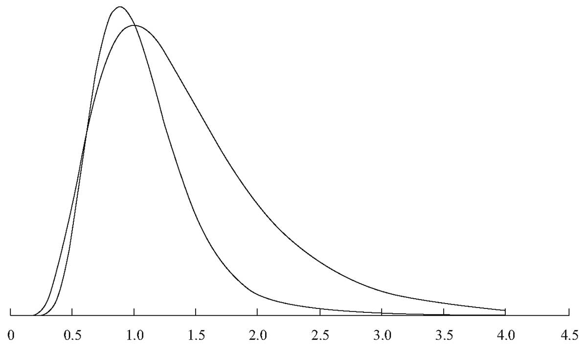 Рисунок 7. Два логнормальных распределения.
Подобно нормальному распределению, логнормальное распределение полностью описывается двумя параметрами. В отличие от других распределений, которые мы рассмотрели, логнормальное распределение определяется в терминах параметров иного распределения.
Два параметра логнормального распределения — это среднее и стандартное отклонение (или дисперсия) связанного с ним нормального распределения: среднее значение и дисперсия ( ln{Y} ), при условии, что величина ( Y ) логнормальна.
Помните, мы должны следить за двумя наборами средних и стандартных отклонений (или дисперсий):
- среднее значение и стандартное отклонение (или дисперсия) связанного нормального распределения (это параметры), и
- среднее значение и стандартное отклонение (или дисперсия) самой логнормальной случайной величины.
Выражения для среднего и дисперсии самой логнормальной величины сложны.
Предположим, что нормальный случайная величина (X) имеет ожидаемое значение ( mu ) и дисперсию ( sigma^2 ).
Определим ( Y = exp (X) ). Помните, что экспоненциальная функция может обозначаться как ( exp (X) ) или ( e^X ), и является операцией, обратной логарифму. Величина ( e approx 2.7182818 ).
Поскольку величина ( Y = ln [ exp (X)] = X ) нормально (мы предполагаем, что (X) нормально), величина (Y) является логнормальной.
Что представляет собой ожидаемое значение ( Y = exp (X) )?
Можно предположить, что ожидаемое значение (Y) это ( exp(mu) ). На самом деле, ожидаемое значение — это ( exp(mu + 0.50sigma^2) ), что больше, чем ( exp(mu) ) на коэффициент ( exp(0.50sigma^2) > 1 ).
Заметим, что ( exp(0.50sigma^2) > 1 ), потому что ( sigma^2 > 0 ).
Чтобы получить некоторое представление об этой концепции, подумайте о том, что произойдет, если мы увеличим ( sigma^2 ). Распределение расширяется; оно может расширяться вверх, но он не может расширяться вниз ниже 0. В результате, центр распределения выталкивается вправо — среднее распределения увеличивается.
Источник этого объяснения: Luenberger (1998).
Выражения для среднего значения и дисперсии логнормальной случайной величины приведены ниже, где ( mu ) и ( sigma^2 ) — среднее и дисперсия соответствующего нормального распределения.
Обращайтесь к этим выражениям по мере необходимости, если нет потребности запоминать их:
- Среднее (( mu_L )) логнормальной случайной величины ( =exp (mu + 0.50sigma^2) )
- Дисперсия (( sigma_L^2 )) логнормальной случайной величины ( =exp (2mu + sigma^2) times [ exp (sigma^2) — 1] )
Теперь мы исследуем взаимосвязь между распределением доходности акций и ценой акций. Далее мы покажем, что если непрерывно начисляемая (т.е. по сложной ставке) доходность акций имеет нормальное распределение, то будущая цена акций будет обязательно логнормально распределена.
Непрерывное начисление означает непрерывную или сплошную временную линию, в отличии от дискретного начисления, при котором время движется в дискретных конечных интервалах.
Непрерывно начисляемая доходность — это одна из так называемых моделей непрерывного финансирования (англ. ‘continuous time finance model’), таких как модель ценообразования опционов Блэка-Шоулза-Мертона.
См. чтения о временной стоимости денег для получения дополнительной информации о непрерывном (сложном) начислении процентов.
Кроме того, мы покажем, что цену акций можно хорошо описать логнормальным распределением, даже если непрерывно начисляемая доходность не следует нормальному распределению. Эти результаты дают теоретическую основу для моделирования цен с помощью логнормального распределения.
Сначала мы покажем, что цена акций в будущий момент времени (T), ( S_T ), равна текущей цене акций, ( S_0 ), умноженной на (e), возведенной в степень ( r_{0,T}), что означает непрерывно начисляемую доходность за временной промежуток от (0) до (T).
Это соотношение выражается как:
( S_T = S_0 exp (r_{0,T}) )
Мы можем записать ( r_{0,T}) как сумму непрерывно начисляемой доходности за более короткие временные периоды, и, если доходность за короткие периоды нормально распределена, то ( r_{0,T}) тоже нормально распределена (при определенных допущениях) или приближенно нормально распределена (без этих допущений).
Так как цена ( S_T ) пропорциональна логарифму нормальной случайной величины, ( S_T ) является логнормальной.
Для того, чтобы создать основу для дальнейшего обсуждения, предположим, что мы имеем ряд последовательных наблюдений стоимости акций (через равные временные периоды):
( S_0, S_1, S_2, ldots , S_T )
Текущая цена акций, ( S_0 ), является известной величиной и поэтому неслучайна. Будущие цены (например, ( S_1 )), однако, являются случайными величинами.
Относительная цена (англ. ‘price relative’), ( S_1 / S_0 ), является отношением конечной цены ( S_1 ) к начальной цене ( S_0 ). Она равна 1 плюс ставка доходности за период владения акцией от (t=0) до (t=1):
( S_1 / S_0 = 1 + R_{0,1} )
Например, если (S_0 = $30) и (S_1 = $34.50 ), то ( S_1 / S_0 = $34.50 / $30 = 1.15). Поэтому, ( r_{0,1} = 0.15 ) или 15%.
В целом, относительные цены имеют вид:
( S_{t+1} / S_t = 1 + R_{t,t+1} )
где
- (R_{t,t+1} ) — ставка доходности за период от ( t ) до ( t+1 ).
Непрерывно начисляемая доходность.
Важной концепцией является непрерывно начисляемая доходность, связанная с доходностью за период владения, такой как ( R_{0,1} ).
Непрерывно начисляемая доходность (англ. ‘continuously compounded return’), связанная с доходностью за период владения, это натуральный логарифм из 1 плюс эта доходность за период владения, или, что эквивалентно, натуральный логарифм из конечной цены деленной на начальную цену (относительная цена).
В этом чтении мы используем строчную (r) для обозначения именно непрерывно начисляемой доходности.
Например, если мы наблюдаем недельную доходность за период владения 0.04, то недельной непрерывно начисляемой доходностью является ( ln (1.04) = 0.039221 ).
€1.00 инвестированный на одну неделю под 0.039221 при непрерывном начислении приносит €1.04, что эквивалентно 4%-ной недельной доходности за период владения.
Формула непрерывно начисляемой доходности для временного промежутка от ( t ) до ( t+1 ):
( large dst r_{t,t+1} = ln (S_{t+1} / S_t) = ln (1 + R_{t,t+1}) ) (Формула 5)
В нашем примере,
( begin{aligned}
r_{0,1} &= ln(S_1/S_0) \
&= ln (1 + R_{0,1}) = ln ($34.50/$30) \
&= ln(1.15) = 0.139762
end{aligned} )
Таким образом, ставка 13.98% является непрерывно начисляемой доходностью во временной промежуток от ( t=0 ) до ( t=1 ). Непрерывно начисляемая доходность меньше соответствующей доходности за период владения.
Если наш инвестиционный временной горизонт простирается от ( t=0 ) до ( t=T ), то непрерывно начисляемая доходность в момент времени ( T ) будет:
( r_{0,T} = ln (S_T / S_0) )
Применив экспоненциальную функцию к обеим сторонам уравнения, мы получим:
( exp(r_{0,T}) = exp[ ln (S_T / S_0)] = S_T / S_0 ),
поэтому
( S_T = S_0 exp (r_{0,T}) )
Мы также можем выразить ( S_T / S_0 ) как произведение относительных цен:
( S_T / S_0 = (S_T / S_{T-1}) (S_{T-1} / S_{T-2}) ldots (S_1 / S_0) )
Логарифмируя обе стороны этого уравнения, мы находим, что непрерывно начисляемая доходность к моменту времени ( Т ) равна сумме ставок непрерывно начисляемой доходности за 1 период:
( large dst
r_{0,T} = r_{T-1,T} + r_{T-2,T-1} + ldots r_{0,1} ) (Формула 6)
Использование доходности за период владения для нахождения конечного значения $1 инвестиции, предполагает умножение величин (1 + доходность за период владения). Использование же непрерывно начисляемой доходности предполагает сложение.
Ключевом предположением во многих инвестиционных задачах является то, что ставки доходности независимо и идентично распределены (IID, от англ. ‘independently and identically distributed’):
- Независимость отражает предположение о том, что инвесторы не могут предсказать будущую доходность, используя прошлую доходность (то есть, это слабая степень эффективности рынка, от англ. ‘weak-form market efficiency’).
- Идентичное распределение отражает предположение о стационарности (то есть, неизменности во времени). Стационарность подразумевает, что среднее и дисперсия доходности не изменяются от периода к периоду.
Предположим, что ставки непрерывно начисляемой доходности за 1 период (например, ( r_{0,1} )) являются IID случайными величинами со средним ( mu ) и дисперсией ( sigma^2 ) (но не делаем предположение о нормальности или других предположений о характере распределения), тогда
( large dst begin{aligned}
{E(r_{0,T})} &= E(r_{T-1,T}) + E(r_{T-2,T-1}) \ &+ ldots E( r_{0,1}) = mu T
end{aligned} ) (Формула 7)
(мы складываем ( mu ) в общей сложности ( T ) раз) и
( large dst sigma^2(r_{0,T}) = sigma^2 T ) (Формула 
(как следствие предположения о независимости).
Дисперсия непрерывно начисляемой доходности за период владения ( T ) равна ( T ), умноженному на дисперсию непрерывно начисляемой доходности за 1 период. Кроме того:
( sigma(r_{0,T}) = sigma sqrt{T} )
Если непрерывно начисляемая доходность за 1 период в правой части Формулы 6 нормально распределяется, то непрерывно начисляемой доходности за период владения ( T ) , ( r_{0,T} ), также нормально распределяется со средним ( mu T ) и дисперсией ( sigma^2 T ).
Эта связь объясняется тем, что линейная комбинация нормальных случайных величин тоже нормальна. Но даже если ставки непрерывно начисляемой доходности за 1 период не являются нормальными, их сумма, ( r_{0,T} ), является приближенно нормальной в соответствии с центральной предельной теоремой.
Мы упоминали центральную предельную теорему (англ. ‘central limit theorem’) ранее, при обсуждении нормального распределения.
Напомним, что в соответствии с центральной предельной теоремой сумма (а также среднее) множества независимых идентично распределенных случайных величин с конечными дисперсиями нормально распределяется, независимо от распределения самих случайных величин.
Центральная предельная теорема обсуждается далее в чтениях о выборочном методе.
[см.: CFA — Центральная предельная теорема и распределение выборочного среднего]
Теперь сравните ( S_T = S_0 exp (r_{0,T}) ) с (Y = exp(Х) ), где ( Х ) является нормальной и Y является логнормальной (как обсуждалось выше).
Ясно, что мы можем моделировать будущую цену акций ( S_T ) как логнормальную случайную величину, поскольку ( r_{0,T} ) должна быть по крайней мере, приблизительно нормально распределена.
Это предположение о нормально распределенной доходности является основой в теории применения логнормального распределения в качестве модели для распределения цен на акций и другие активы.
Волатильность.
Непрерывно начисляемая доходность играет роль во многих моделях ценообразования опционов, как уже упоминалось ранее. Оценка волатильности имеет решающее значение для использования моделей ценообразования опционов, таких как модель Блэка-Шоулза-Мертона.
Волатильность (англ. ‘volatility’) оценивает стандартное отклонение непрерывно начисляемой доходности базового актива.
Волатильность также называют мгновенным стандартным отклонением, и обозначают так же: ( sigma ). Базовый актив в данном случае — это актив, лежащий в основе опциона.
Для получения более подробной информации об этих концепциях см. Chance and Brooks (2012).
На практике мы очень часто оцениваем волатильность, используя историческую последовательность непрерывно начисляемой дневной доходности. Мы собираем множество ставок непрерывно начисляемой доходности (за период владения 1 день), и затем используем Формулу 5, чтобы преобразовать их в непрерывно начисляемую дневную доходность.
Затем мы вычисляем стандартное отклонение непрерывно начисляемой дневной доходности и аннуализируем (пересчитываем в годовое исчисление) это значение с помощью Формулы 8.
Для вычисления стандартного отклонения множества или выборки из (n) ставок доходности, мы суммируем квадраты отклонения каждой ставки доходности от средней доходности, а затем делим эту сумму на ( n — 1 ) (см. Формулу 13 ). В результате получается выборочная дисперсия.
Квадратный корень из выборочной дисперсии дает нам стандартное отклонение выборки. Более подробно расчет стандартного отклонения рассмотрен в чтениях о статистических концепциях и доходности рынка.
По соглашению, волатильность указывается в годовом исчислении.
В финансовой практике годовое исчисление часто рассчитывается на базе 250 дней в году — это приблизительное количество дней, когда финансовые рынки открыты для торговли. База в 250 дней в году может привести к лучшей оценке волатильности, чем календарная база — в 365 дней.
Таким образом, если дневная волатильность была 0.01, мы можем выразить волатильность (в годовом исчислении) как ( 0.01 sqrt{250} = 0.1581 ).
Пример 10 иллюстрирует оценку волатильности акций Astra International.
Пример (10) оценки волатильности в соответствии с моделью ценообразования опционов.
Предположим, вы анализируете акции компании Astra International (обозначение на индонезийской фондовой бирже: ASII) и вас интересует цена акций Astra за неделю, в течение которой международные экономические новости существенно повлияли на индонезийский фондовый рынок.
Вы решили использовать волатильность в качестве меры изменчивости акций Astra в течение этой недели. Таблица 7 показывает цены закрытия (цены на момент закрытия биржи) в течение этой недели.
|
Дата |
Цена закрытия (IDR) |
|---|---|
|
17 июня 2013 |
6,950 |
|
18 июня 2013 |
7,000 |
|
19 июня 2013 |
6,850 |
|
20 июня 2013 |
6,600 |
|
21 июня 2013 |
6,350 |
Используйте данные из Таблице 7, чтобы сделать следующее:
- Оцените волатильность акций Astra. (Пересчитайте волатильность в годовое исчисление на основе 250 дней в году.)
- Определите распределение вероятностей для цен на акции Astra, если непрерывно начисляемая дневная доходность следует нормальному распределению.
Решение для части 1:
Во-первых, используйте Формулу 5 для расчета непрерывно начисляемой дневной доходности. Затем найдите стандартное отклонение для полученной доходности обычным способом. (При расчете выборочной дисперсии, чтобы получить стандартное отклонение выборки, используйте в знаменателе размер выборки, уменьшенный на 1).
( ln(7,000/6,950) = 0.007168 )
( ln(6,850/7,000) = -0.021661 )
( ln(6,600/6,850) = -0.037179 )
( ln(6,350/6,600) = -0.038615 )
Сумма = -0.090287
Среднее = -0.022572
Дисперсия = 0.000452
Стандартное отклонение = 0.021261
Стандартное отклонение непрерывно начисляемой дневной доходности равно 0.021261.
Формула 8 утверждает, что ( hat{sigma} (r_{0,T}) = hat{sigma} sqrt{T} ). В этом примере ( hat{sigma} ) является стандартным отклонением выборки для непрерывно начисляемой доходности за 1 период. Таким образом, ( hat{sigma} ) соответствует 0.021261.
Мы хотим пересчитать результат в годовое исчисление так, чтобы временной горизонт ( T ) соответствовал одному году. Так как ( hat{sigma} ) исчисляется в днях, мы устанавливаем ( T ) равным количеству торговых дней в году (250).
Мы находим, что в годовом исчислении волатильность акций Astra за эту неделю составляла 33.6%, что рассчитывается как ( 0.02126 sqrt{250} = 0.336165 ).
Обратите внимание, что выборочное среднее, -0.022572, является возможной оценкой среднего значения, ( mu ), для непрерывно начисляемой доходности за 1 период или ставок дневной доходности.
Выборочное среднее может быть переведено в оценку ожидаемой непрерывно начисляемой годовой доходности с помощью Формулы 7: ( hat{mu} T = -0.022572 (250) ) (используется база в 250 дней, чтобы результат соответствовал расчету волатильности).
Но четырех наблюдений слишком мало, чтобы оценить ожидаемую доходность. Изменчивость дневной доходности важнее любой информации об ожидаемой доходности в такой короткой последовательности наблюдений.
Решение для части 2:
Цены на акции Astra должны следовать логнормальному распределению, если непрерывно начисляемая дневная доходность акций Astra следует нормальному распределению.
Мы показали, что распределение цены акций является логнормальным, с учетом некоторых предположений.
Каковы среднее значение и дисперсия ( S_T ), если ( S_T ) следует логнормальному распределению?
Выше мы привели перечень выражений для среднего и дисперсии логнормальной случайной величины. В этом перечне, ( hat{mu} ) и ( hat{sigma} ) ссылаются, в контексте этого обсуждения, на среднее и дисперсию временного горизонта ( T) (а не одного периода) непрерывно начисляемой доходности (предполагая, что оно следует нормальному распределению), совместимому с временным горизонтом ( S_T ).
Например, выражение для среднего значения:
( E(S_T) S_0 exp[E(r_{0,T}) + 0.5sigma^2(r_{0,T})] ).
Ранее в этом чтении мы использовали среднее значение и дисперсию (или стандартное отклонение), чтобы построить интервалы, в которых мы ожидали найти определенный процент наблюдений нормально распределенной случайной величины. Эти интервалы были симметричны относительно среднего значения.
Можем ли мы использовать подобные, симметричные интервалы для логнормальной случайной величины?
К сожалению, мы не можем. Поскольку логнормальное распределение не является симметричным, такие интервалы являются более сложными, чем для нормального распределения, и мы не будем обсуждать эту особую тему здесь.
См. Hull (2011) для обсуждения логнормальных доверительных интервалов.
Наконец, мы представили связь между средним и дисперсией непрерывно начисляемой доходности с различными временными горизонтами (см. Формулы 7 и 8), но как связаны средние и дисперсии ставок доходности за период владения и ставок непрерывно начисляемой доходности?
Как аналитики, мы обычно рассуждаем в терминах доходности за период владения, а не непрерывно начисляемой доходности, и хотим преобразовать средние и стандартные отклонения доходности за период владения в средние и стандартные отклонения непрерывно начисляемой доходности для работы с опционами, например.
Чтобы осуществить такие преобразования (и в таком и в обратном направлении), мы можем использовать выражения, изложенные в работе: Ferguson (1993).
Что такое Логнормальное распределение?
Логарифмическое нормальное распределение – это статистическое распределение логарифмических значений из соответствующего нормального распределения. Логарифмически нормальное распределение можно преобразовать в нормальное распределение и наоборот, используя соответствующие логарифмические вычисления.
Понимание нормального и логнормального
Нормальное распределение – это распределение вероятностей результатов, которое является симметричным или образующим кривую колокола. При нормальном распределении 68% результатов попадают в одно стандартное отклонение, а 95% – в два стандартных отклонения.
Хотя большинство людей знакомы с нормальным распределением, они могут быть не так знакомы с лог-нормальным распределением. Нормальное распределение можно преобразовать в логарифмическое распределение с помощью логарифмической математики. Это прежде всего основа, поскольку логнормальное распределение может происходить только из нормально распределенного набора случайных величин.
Может быть несколько причин для использования логнормальных распределений в сочетании с нормальными распределениями. Как правило, большинство логнормальных распределений являются результатом натурального логарифма, где основание равно e = 2,718. Однако логнормальное распределение можно масштабировать с использованием другой базы, которая влияет на форму логнормального распределения.
В целом логнормальное распределение отображает логарифм случайных величин из кривой нормального распределения. В общем, журнал известен как показатель степени, до которого необходимо возвести базовое число, чтобы получить случайную величину (x), которая находится вдоль нормально распределенной кривой.
Для получения дополнительной информации см. Также статью Investopedia « Логнормальное и нормальное распределение».
Применение и использование логнормального распределения в финансах
Нормальные распределения могут представлять несколько проблем, которые могут решить логнормальные распределения. В основном нормальные распределения могут допускать отрицательные случайные величины, в то время как логнормальные распределения включают все положительные переменные.
Одним из наиболее распространенных приложений, где в финансах используются логнормальные распределения, является анализ цен на акции . Потенциальную доходность акции можно изобразить в виде нормального распределения. Тем не менее, цены на акции можно изобразить в виде логарифмически нормального распределения. Таким образом, кривая нормального логарифмического распределения может использоваться для более точного определения совокупной доходности, которую акция может ожидать за определенный период времени.
Обратите внимание, что логнормальные распределения имеют положительный перекос с длинными правыми хвостами из-за низких средних значений и высокой дисперсии случайных величин.
Логнормальное распределение в Excel
Логнормальное распределение можно выполнить в Excel . Он находится в статистических функциях как ЛОГНОРМ.РАСП.
Excel определяет это как следующее:
ЛОГНОРМ.РАСП (x; среднее; стандартное_откл; совокупное)
Возвращает логнормальное распределение x, где ln (x) нормально распределено с параметрами mean и standard_dev.
Для расчета ЛОГНОРМ.РАСП в Excel вам понадобится следующее:
x = значение, при котором оценивается функция
Среднее = среднее значение ln (x)
Стандартное отклонение = стандартное отклонение ln (x), которое должно быть положительным.
Логнормальное распределение непрерывной случайной величины.
Одним из самых
близких к нормальному распределению
является логнормальное распределение,
имеющее слабую левую асимметрию и
относящееся ко второму типу распределений.
Очевидно, что многие геохимические
компоненты не подчиняются нормальному
распределению, например концентрация
селена в растительном материале,
концентрация йода в грунтовых водах
подчиняются асимметричным распределениям.
Кривая логнормального распределения
отражена на рисунке.
Существуют две
физические причины асимметричности.
Первая причина кроется в пороге
чувствительности приборов, определяющих
концентрацию редких химических элементов
(селен, радий и др.). Левая асимметричность
возникает, из-за того, что много данных
концентрируется около порога
чувствительности, и если бы этого порога
не было, то распределение приняло бы
нормальный симметричный вид.
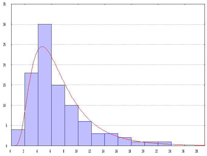
Рис. Кривая логнормального
распределения.
Вторая причина
кроется в детерминированности изменений
природных объектов, тем более мощные
геохимические и тектонические процессы,
которые протекали при формировании
залежей полезных ископаемых, тем более
кривая распределения характеристик
этих залежей будет асимметричной.
Асимметричность, например, возникает,
если толкать спортсмена-стрелка в тире
в момент выстрела, в этом случае пули
на мишени будут располагаться
преимущественно с одной стороны мишени.
Если результаты наблюдений, распределение
которых представлено на рисунке,
прологарифмировать (то есть вместо
переменной xi
использовать переменную y
= log
xi),
то распределение прологарифмированной
переменной примет нормальный вид. Все
перечисленные ранее параметры и
статистики также характерны и пригодны
и для логнормального распределения. На
практике они рассчитываются по тем же
формулам, только предварительно все
значения выборки логарифмируются,
однако основные статистики можно
посчитать, используя и не преобразованные
данные, в этом случае среднеарифметическому
значению будет соответствовать
геометрическое среднее, а значению
дисперсии будет соответствовать
геометрическая дисперсия. Преобразования
типа y
= log
xi
широко применяются в геологии, однако
известно (У.Крамбейн, Ф.Грейбилл) и так
называемое фи — преобразование — φ
= — log
xi.
Это преобразование используется,
например, при изучении распределений
размеров частиц осадочных пород.
Лекция 8.
Гамма-распределение непрерывной случайной величины и его разновидность — распределение Пуассона непрерывной случайной величины.
Гамма — распределение
относится по классификации Пирсона к
третьему типу кривых, в этот тип входит
обширная группа асимметричных
распределений (в том числе и бета –
распределение). Данные, которые подчиняются
этим распределениям, никакими
преобразованиями не могут быть
преобразованы таким образом, чтобы
после они имели нормальное распределение.
Однако одна из разновидностей гамма —
распределения имеет для нас значение,
так как существуют способы преобразования
данных, после которых они могут подчиняться
логнормальному и нормальному распределению.
Плотность вероятности гамма — распределения
описывается следующей формулой
G (x;Γ;β)
= xr-1*e-χ/β/
Γ(г)
βr
x≥0, r >0, β>0.
Дополнительными
параметрами гамма — распределения
являются величины r
и β,
первый является параметром положения,
а второй параметром масштаба.

Рис Примеры кривых плотности
вероятности, соответствующие различным
значениям r, при β
= 1.
Выбор гамма
распределения в качестве модели
распределения изучаемой совокупности
определяется наличием у изучаемой
кривой распределения так называемого
хвоста, являющегося следствием
асимметричности распределения и
препятствующим различным математическим
преобразованиям привести экспериментальные
данные к нормальному или логнормальному
распределению. Так же как и для нормального
распределения плотности вероятности
распределения, выраженные через площади
под кривой распределения, давно рассчитаны
и опубликованы в таблицах. Вычислить и
оценить параметры —
r
и β
можно по таблицам Сиддикуи и Вейса и
через них рассчитать μ и σ2
(то есть истинное среднее совокупности
и ее дисперсию) по формулам
μ = β*
r;
σ2=
β2*
r.
Как видно из этих
формул, для гамма — распределений
отмечается сильная зависимость между
средним и дисперсией, тогда как в случае
нормального распределения такой
зависимости нет.
Основные компоненты
полиметаллических месторождений,
месторождений цветных металлов и золота
могут подчиняться разновидностям гамма
– распределения. Частным случаем, гамма
распределений является распределение
Пуассона, если его использовать для
анализа непрерывных случайных величин.
Особенно это распределение характерно
для месторождений золота, так как именно
в большей части на этих месторождениях
часты находки самородков золота (редкие
события) или можно перефразировать —
встречаются пробы с аномальным высоким
содержанием золота (ураганные пробы),
во много раз превышающим наиболее
распространенные содержания металла
по конкретному месторождению (эффект
самородков). Несмотря на то, что гамма
— распределения, в том числе и распределение
Пуассона хорошо изучены на практике,
специалисты стараются не использовать
эту модель для оценки истинных параметров
изучаемой совокупности из-за ряда
причин, в том числе и из-за сильной
зависимости между средним и дисперсией.
Для решения этой задачи общепринят иной
подход, при котором эффект самородков
стараются нейтрализовать и затем после
возможных преобразований данных
предположить нормальную модель их
распределения.
Учет ураганных
проб.
Сама проблема
ураганных проб предполагает две стадии
ее решения, в первую стадию, нужно выявить
ураганные пробы, а во вторую стадию их
нейтрализовать. Существует много
способов регистрации ураганных проб,
и они подробно описаны в специализированной
литературе [ 5 ]. Однако в последнее
время среди специалистов наибольшую
популярность получили “квантильный”
способ обнаружения ураганных значений
металлов в пробах и способ обнаружения
ураганных проб по излому на кумулятивной
кривой распределения, описанные в книге
Ю.Е. Капутина “Горные компьютерные
технологии и геостатистика”. Если
придерживаться терминологии предложенной
в этих лекциях, то первый способ можно
назвать децильным способом, так как
массив проб сначала сортируется по
величине содержания металла от
минимального до максимального, затем
строится частотная таблица и гистограмма.
А после таблица разделяется на заданное
количество квантилей, обычно на 10 частей
(то есть массив разделяется на децили).
В результате формируется таблица, пример
которой приведен ниже.
|
Класс |
Число |
Среднее |
Минимум |
Максимум |
Доля металла с данным содержанием от |
Доля |
|
0-10 |
1110 |
0.004 |
0.000 |
0.010 |
4.805 |
0.07% |
|
10-20 |
1110 |
0.010 |
0.010 |
0.018 |
11.522 |
0.16% |
|
20-30 |
1110 |
0.021 |
0.018 |
0.030 |
23.816 |
0.34% |
|
30-40 |
1110 |
0.035 |
0.030 |
0.049 |
38.823 |
0.55% |
|
40-50 |
1110 |
0.052 |
0.049 |
0.060 |
57.571 |
0.82% |
|
50-60 |
1110 |
0.080 |
0.060 |
0.100 |
88.946 |
1.27% |
|
60-70 |
1110 |
0.128 |
0.100 |
0.160 |
141.922 |
2.02% |
|
70-80 |
1110 |
0.219 |
0.160 |
0.290 |
243.590 |
3.47% |
|
80-90 |
1110 |
0.426 |
0.290 |
0.640 |
472.534 |
6.73% |
|
90-100 |
1106 |
5.370 |
0.640 |
305.310 |
5938.771 |
84.57% |
|
ВСЕГО |
11096 |
0.633 |
0.000 |
305.310 |
7022.301 |
100.00% |
|
90-91 |
111 |
0.677 |
0.640 |
0.720 |
75.161 |
1.27% |
|
91-92 |
111 |
0.777 |
0.720 |
0.840 |
86.204 |
1.45% |
|
92-93 |
111 |
0.896 |
0.840 |
0.950 |
99.474 |
1.67% |
|
93-94 |
111 |
1.029 |
0.950 |
1.120 |
114.198 |
1.92% |
|
94-95 |
111 |
1.238 |
1.120 |
1.390 |
137.390 |
2.31% |
|
95-96 |
111 |
1.587 |
1.390 |
1.790 |
176.153 |
2.97% |
|
96-97 |
111 |
2.046 |
1.790 |
2.350 |
227.100 |
3.82% |
|
97-98 |
111 |
2.899 |
2.360 |
3.690 |
321.840 |
5.42% |
|
98-99 |
111 |
5.497 |
3.700 |
8.660 |
610.180 |
10.27% |
|
99-100 |
107 |
38.234 |
8.670 |
305.310 |
4091.070 |
68.89% |
|
ВСЕГО |
1106 |
5.370 |
0.640 |
305.310 |
5938.770 |
100.00% |
Если последний
класс (90-100%) содержит долю металла,
большую чем 40% от общего количества, то
считается, что в массиве данных существуют
ураганные пробы. Далее рассчитывается
аналогичная таблица для последнего
класса. Границей для ураганных проб
считается минимальное содержание
первого класса, содержащего долю металла
более 10%. В данном примере – это 3.7 г/т.
Считается, что подобный анализ нужно
проводить для каждого типа руд, и для
каждого участка месторождения. На
практике отмечается много случаев,
когда границы ураганных проб на одном
и том же месторождении резко отличались
друг от друга на разных его участках.
Второй способ
состоит в том, что строится кумулятивное
распределение массива данных, но
отображается оно в виде огивы и исследуется
конечная часть хвоста распределения.
На графике отмечается место перегиба
кумулятивной кривой, которое и является
границей, после которой фиксируются
ураганные пробы.

Рис
. Определение границы, после которой
фиксируются ураганные пробы по месту
излома огивы (вместо накопленных частот
по оси абсцисс фиксируются соответствующие
номера проб).
Существуют еще
более простые методы выявления ураганных
проб, можно например, просто определить
ураганные пробы в хвосте массива
распределения, после достижения 95% или
99% накопленных частот или использовать
соотношение между модой, медианой и
среднеарифметическим значением которое,
характерно для умеренно асимметричных
кривых —
Mo–
χ=3(Me
– χ).
Есть несколько
подходов и к нейтрализации ураганных
проб.
-
Можно исключить
аномальные значения из выборки (например,
просто отрезать хвост распределения
после достижения 95%-99% накопленных
частот). -
Можно вместо
аномальных значений указать пороговые
значения, при которых выборочные данные
будут иметь нормальное или логнормальное
распределение. -
Можно присвоить
аномальным значениям среднеарифметические
значения выборки.
Подразумевается,
что в первом и третьем случае, после
процедур данные будут иметь нормальное
или логнормальное распределение. Однако
вопрос и о способах выявления и о
необходимости нейтрализации ураганных
проб остается открытым, так как в любом
случае, мы можем допустить еще большую
ошибку при оценке истинных параметров,
как всей изучаемой совокупности, так
и ее частей. Так, например, нейтрализация
ураганных проб в выборке, при разведке
месторождений золота может уменьшить
оценку запасов месторождения, но главное
значительно ухудшить экономическую
оценку месторождения, из-за высокой
цены на этот металл. Тем не менее,
большинство специалистов соглашаются,
что лучшим выбором для оценки параметров
будет выбор нормальной модели распределения
выборочных данных. То есть наши оценки
параметров будут более точными, чем
ближе к нашему экспериментальному
распределению будет подходить нормальная
модель распределения.
Кроме логарифмирования
данных и нейтрализации ураганных проб
можно предложить и другие полезные
преобразования данных, после которых
наши данные могут быть ближе к нормальному
распределению. Одно из таких преобразований
это преобразование типа — yi=√xi
и оно в ряде случаев может привести к
сокращению пуассоновского хвоста, если
наблюдаемые значения близки к 0, то
используют преобразование типа — yi=√xi
+1/2. Можно использовать также и степенные
преобразования, в этом случае больше
будут увеличиваться большие значения,
чем малые, ко всему прочему это
преобразование позволяет лучше читать
каротажные диаграммы.
Соседние файлы в предмете [НЕСОРТИРОВАННОЕ]
- #
- #
- #
- #
- #
- #
- #
- #
- #
- #
- #
Всем привет.
В тот раз мы разобрались с темой нормального распределения, а сегодня попытаемся для себя разобраться с новой темой, еще более интересной. Она очень важная, поэтому будет много текста из книги Натенберга.
Насколько обосновано наше предположение, что цены базового актива распределены нормально? Даже если не касаться самой возможности существования какого-либо строгого распределения цен в реальной жизни, то можно утверждать, что у допущения о нормальном распределении есть один серьезный недостаток. Кривая нормального распределения симметрична. Если принимается допущение о нормальном распределении, то мы, предположив возможность повышательного изменения цены БА, обязаны предположить возможность такого же понижательного изменения. Если мы допускаем возможность повышения цены РИ при прайсе 70 000 пунктов на 80 000 пунктов вверх до 150 000, то должны допустить также и возможность падения до -10 000 пунктов. Поскольку РИ это не WTI и цены не могут уйти в отрицательную зону, становится очевидным, что допущение о нормальном распределении не вполне корректно. Как устранить этот недостаток?
До сих пор мы определяли волатильность как процентное изменение цены базового актива. В этом смысле процентная ставка и волатильность схожи, поскольку и то и другое дает представление о доходности. Основное различие между ними заключается в том, что процентный доход положителен, в то время как волатильность отражает как положительное, так и отрицательные доходности. Если вложить деньги под фиксированную ставку, то сумма всегда увеличивается. Но если вложить их в БА с волатильностью больше нуля, то цена этого инструмента может как повыситься, так и понизиться. Волатильность, определяемая как стандартное отклонение процентных изменений цены БА ничего не говорит о направлении изменения цены.
Поскольку волатильность отражает доходность, большое значение имеет порядок расчета доходности. Предположим, что мы инвестировали 1000 $ на год под 12% годовых. Сколько мы получим в конце года? Ответ зависит от того, как будут выплачиваться проценты:

Когда проценты выплачиваются чаще, даже если годовая ставка не меняется, доходность увеличивается. В случае непрерывной выплаты процентов доходность будет максимальной (здесь используются сложные проценты, непрерывное начисление означает, что интервал между выплатами становится все меньше и меньше, в предельном случае — бесконечно малым, при этом рост суммы описывается функцией exp(r*t)).
Теперь самое интересное, проделаем те же расчеты для отрицательной процентной ставки, хотя она встречается реже. Предположим, что мы ежегодно теряем 12% инвестиций от первоначальной суммы 1000 $. Сколько у нас останется в конце года? Ответ зависит от того, как часто начисляются убытки:

В случае отрицательной процентной ставки убытки, как и отрицательная доходность, меньше, если убытки начисляются чаще, хотя годовая ставка остается неизменной.
Точно так же, как процентные выплаты могут начисляться с разными интервалами и давать различные эффективные доходности, так и волатильность может рассчитываться с разными интервалами. Для целей оценки опциона делается допущение, что цена БА меняется непрерывно (как вверх, так и вниз), а волатильность «накапливается» непрерывно со скоростью, соответствующей годовой волатильности данного БА (если точнее, то непрерывно накапливается не волатильность, а дисперсия, поэтому волатильность увеличивается пропорционально корню квадратному из времени).
Что произойдет, если в каждый момент времени цена БА будет повышаться или понижаться на заданный процент, а распределение этих движений будет нормальным? Если исходить из нормального распределения изменений цены БА, то в результате непрерывного накопления этих изменений мы получим к дате экспирации логнормальное распределение цен. Такое распределение смещено из-за того, что движения цены вверх в абсолютном выражении больше движений цены вниз (см.внизу рисунок). В нашем примере с 12%-ой ставкой непрерывного начисления положительного процента даст через год +127,50 $, в то время, как непрерывное начисление убытка по той же ставке отнимет -113,08 $. Хотя в среднем относительные колебания цены (доходности), взятые по абсолютной величине, и сохраняются на уровне 12%, непрерывное 12%-ое нарастание и снижение приводит к различным повышательным и понижательным изменениям цены.
Модель Блэка-Шоулза — это модель непрерывного времени. Она исходит из того, что волатильность БА в течение всего срока действия опциона постоянна, но эта волатильность рассчитывается по методу непрерывного начисления. Эти два допущения означают, что возможные цены БА распределяются логнормально. Это также объясняет, почему у опционов с более высоким страйком стоимость больше, чем у опциона со страйком пониже, когда обе цены как будто одинаково далеки от текущей цены БА.
Здесь ВНИМАНИЕ! Я собственными глазами видел, когда цены по равноудаленным страйкам от текущей цены БА были одинаковыми. И такое бывает очень часто. Вопрос аудитории на засыпку: почему так бывает?
Предположим, что цена фьюча РИ составляет ровно 100 000. Если мы принимаем во внимание нормальное распределение возможных цен, то 110 колл и 90 пут, которые оба вне денег на 10%, должны иметь одинаковую теоретическую стоимость. Но если мы допускаем в модели Блэка-Шоулза логнормальное распределение, то стоимость 110 колла всегда будет выше стоимости 90 пута. Логнормальное распределение предполагает более значительное в абсолютном выражении повышательное изменение цены.
Таким образом, для 110 колла характерна более высокая вероятность роста цены, чем для 90 пута. Сноска на полях: конечно же это только в теории, а на практике нет никакого закона, который гласил бы, что рыночная цена 90 пута не может превысить цену 110 колла.

Встроенное в модель Блэка-Шоулза допущение о логнормальном распределении устраняет сформулированную ранее логическую проблему. Если мы допустим возможность неограниченного повышения цены БА, то в случае нормального распределения придется допустить и ее неограниченное понижательное изменение. Это приводит к появления отрицательных цен БА, что исключено для большинства рассматриваемых нами инструментами (Натенберг не видел как WTI на Мосбирже торговался в недавнем времени, он бы посмеялся). Логнормальное распределение допускает возможность неограниченного роста цены (логарифм +бесконечноть = +бесконечность), но исключает возможность ее падения ниже нуля (логарифм -бесконечность = 0). Вообще такая формулировка некорректна с математической точки зрения, но Натенберг почему-то пишет именно так.
Логарифмическая функция берется всегда от положительных значений, так было бы писать правильно, но саму идею Натенберг очень красиво изложил, логнормальное распределение чаще встречается в реальной жизни, потому что цена на товар не может быть отрицательной, если не считать WTI.
Не лишним будет также вспомнить про саму функцию логарифма и ее свойства:

В заключение подведем итог и перечислим важнейшие допущения в отношении изменения цены, встроенные в модель Блэка-Шоулза:
- Изменение цены БА носит случайный характер и на него невозможно воздействовать, как невозможно предсказать заранее направление этого изменения.
- Процентные изменения цены БА имеют нормальное распределение.
- Поскольку мы принимаем, что процентные изменения цены БА накапливаются непрерывно, цены БА при экспирации распределяются логнормально.
- Математическое ожидание данного логнормального распределения — это форвардная цена БА.
При этом, первое допущение может вызвать у многих трейдеров акт агрессии и возражения, ведь как так? Технические аналитики полагают, что, анализируя прошлую динамику цен, можно предсказать направление их будущего изменения. Можно на графике построить уровни поддержки и сопротивления, найти ГИП и другие фигуры графического анализа и они ведь действительно работают и помогают предсказать тенденцию изменения цены. Но в случае классических опционщиков всё это не важно, потому что модель Блэка-Шоулза исходит из случайного изменения цен и невозможности предсказания направления их изменения. Это не означает, что использование модели Блэка-Шоулза не требует прогнозирования, однако, главная задача такого прогнозирования — предсказать величину изменения цены, а не направление изменения. Это и есть торговля волатильностью — покупай дешево и продавай дорого.
Как мы увидим дальше, есть основания сомневаться и в правомерности третьего допущения о логнормальном распределении цен при экспирации. Для одних рынков оно правомерно, для других — нет. Здесь опять-таки важно, чтобы использующий модель трейдер знал, какие допущения принимаются при расчете теоретической стоимости опциона, тогда он сможет решить насколько точны эти допущения, а, следовательно, и полученные значения теоретической стоимости.
Если такие вот топики вам заходят, ставьте лайки и жмите колокольчик.
С уважением, Карлсон.
—
p.s. кому интересно, свои мысли по рынку кидаю в канал «Фондовый рынок глазами Карлсона» (t.me/KarLsoH), там же есть и опционный чат.
Рассмотрим Логнормальное распределение. С помощью функции MS EXCEL
ЛОГНОРМ
.РАСП()
построим графики функции распределения и плотности вероятности. Сгенерируем массив случайных чисел, распределенных по логнормальному закону, произведем оценку параметров распределения, среднего значения и стандартного отклонения.
Если случайная величина Х имеет
логнормальное распределение
(англ.
Lognormal
distribution
)
, то её логарифм Y=LN(X) имеет
нормальное распределение
. Справедливо и обратное утверждение: если случайная величина Y имеет
нормальное распределение
, то случайная величина X=EXP(Y) имеет
логнормальное распределение
. Из свойства логарифма следует, что X>0.
Сначала рассмотрим связь между
нормальным
и
логнормальным
распределениями.
Как известно,
нормальное распределение
чаще всего рассматривается как подходящая модель для описания такого процесса, когда действует большое число независимых случайных причин. Например, при производстве кускового мыла, вес каждого куска немного отличается от заданного в силу множества случайных причин, действующих на процесс: колебания температуры, состава исходного сырья, скачки напряжения на оборудовании и др. В этом случае плотность распределения случайной величины «вес мыла» имеет симметричную, колоколообразную форму.
Однако, в некоторых случаях наблюдения показывают, что случайная величина имеет заметно скошенное (несимметричное) распределение (см. раздел
Ассиметричность
в статье
Описательная статистика в MS EXCEL
), и, соответственно, не может быть описана
нормальным распределением
.
Скошенные распределения
имеют место когда, случайные величины не могут быть отрицательными или имеется другая естественная граница (не может быть меньше определенного значения).
Логнормальное распределение
является одним из примеров
скошенного распределения
.
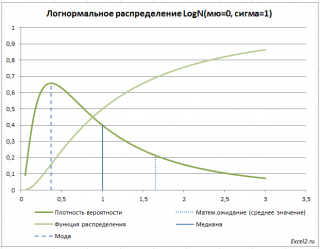
В чем же состоит различие в процессах, приводящих к
нормальному
или
логнормальному
распределениям? Оба распределения имеют место, когда на описываемый объект воздействует множество случайных и независимых факторов. Если воздействия каждого из факторов складываются, т.е. имеется аддитивный характер их взаимодействия, то имеет место
нормальное распределение
(см. статью про
Центральную предельную теорему
).
Если воздействия каждого из факторов не складываются, а перемножаются, т.е. имеется мультипликативный характер взаимодействия, что часто соответствует
Логнормальному распределению.
Факторы также независимы как и в случае нормального распределения, но эффект от их воздействия накапливается в объекте в зависимости от предыдущего их количества.
Чтобы это пояснить, рассмотрим процесс износа подшипника. Понимание физического процесса позволит построить адекватную статистическую модель (распределение) и, в данном случае, оценить средний срок его работы до поломки.
Износ подшипника происходит из-за множества случайных независимых факторов: несовершенства формы шариков подшипника, внешних ударов, попадания грязи и пр. Пусть в определенный момент происходит случайное событие, например, удар, который приводит к микродефекту внешнего кольца удерживающего шарики, но поломка подшипника еще не происходит. Понятно, что с деформированным кольцом разрушение подшипника ускорится (например, за счет повышенного истирания). Теперь рассмотрим два вида взаимодействия воздействующих факторов: аддитивный и мультипликативный.
В первом случае, считается, что микродефекты просто складываются и поломка подшипника происходит при превышении некого порогового их воздействия (суммирование микродефектов). Т.е. в этой модели не учитывается, что каждый последующий микродефект воздействует уже не на новый подшипник, а на поврежденный.
Во втором случае (мультипликативное взаимодействие),
каждый последующий микродефект воздействует на подшипник пропорционально его текущему состоянию.
Т.е. одно и тоже воздействие будет приводить к разным последствиям (дефектам) в случае нового или уже поврежденного подшипника.
Как было сказано выше, модель аддитивного взаимодействия случайных факторов приводит к
нормальному распределению
(в данном случае она не применима для оценки срока работы подшипника). В нашем случае более адекватной моделью является модель мультипликативного взаимодействия, когда учитывается не только случайное воздействие фактора, но и состояние самой системы, на которую действует фактор. Мультипликативный эффект от всех случайных независимых воздействий на подшипник аккумулируется до тех пор пока не произойдет его разрушение.
Попытаемся вышесказанное изложить с помощью формул. По аналогии с
ЦПТ
и учитывая свойство логарифма
LN
(
x
1*
x
2*…*
xn
)=
LN
(
x
1)+
LN
(
x
2)+…
+LN(x
n
)
, можно предположить, что если x1, x2, x3, … xn – случайные независимые величины, и
y
=
x
1*
x
2*
x
3* … *
xn
, то случайная величина LN(y) будет распределена по
нормальному закону
. Если это условие выполняется, т.е.
LN
(
y
)
~
N
(μ;σ)
, то
y
имеет
логнормальное распределение
с параметрами μ и
σ
.
Примерами, когда имеет место
логнормальное распределение
могут служить следующие ситуации:
- сбой из-за химических реакций или деградации, таких как коррозия или диффузия, которые являются частой причиной отказа полупроводникового элемента;
- время до разрушения в металлах при условии роста усталостных трещин.
Ниже приведена функция плотности
логнормального распределения
:
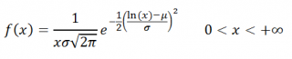
СОВЕТ
: Подробнее о
Функции распределения
и
Плотности вероятности
см. статью
Функция распределения и плотность вероятности в MS EXCEL
.
Обратите внимание, что хотя μ и
σ
являются параметрами распределения, они НЕ являются
средним значением
(обозначим как μ*) и
стандартным отклонением
(
σ
*) этого распределения (как у
нормального распределения
).
Ниже приведены формулы для расчета
среднего
и
стандартного отклонения логнормального распределения
.
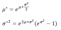
Примечание
: μ и
σ
являются параметрами
нормального распределения
LN(y) и, соответственно, его
средним
и
стандартным отклонением
.
Логнормальное распределение в MS EXCEL
В MS EXCEL, начиная с версии 2010, для
Логнормального распределения
имеется функция
ЛОГНОРМ.РАСП()
, английское название — LOGNORM.DIST(), которая позволяет вычислить плотность вероятности (см. формулу выше) и
интегральную функцию распределения
(вероятность, что случайная величина X, распределенная по
логнормальному закону
, примет значение меньше или равное x). Вычисления в последнем случае производятся по следующей формуле:
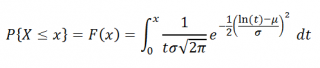
Логнормальное распределение
имеет обозначение Ln
N
(μ;
σ
).
Примечание
: До MS EXCEL 2010 в EXCEL была функция
ЛОГНОРМРАСП()
, которая также позволяет вычислить
кумулятивную (интегральную) функцию распределения
, но не позволяет вычислить
плотность вероятности
.
ЛОГНОРМРАСП()
оставлена в MS EXCEL 2010 для совместимости. В
файле примера на листе Пример
приведены несколько альтернативных формул для вычисления
плотности вероятности
и
интегральной функции распределения
(использованы функции
НОРМ.СТ.РАСП()
и
НОРМ.РАСП()
.
Примечание
: Для удобства написания формул в
файле примера
созданы
Имена
для параметровраспределения: μ и
σ
.
Графики функций
В
файле примера
приведены графики
плотности распределения вероятности
и
интегральной функции распределения
.
Примечание
: Для построения
функции распределения
и
плотности вероятности
можно использовать диаграмму типа
График
или
Точечная
(со сглаженными линиями и без точек). Подробнее о построении диаграмм читайте статью
Основные типы диаграмм
.
Генерация случайных чисел
Для генерирования массива чисел, распределенных по
логнормальному закону
, можно использовать формулу
=ЛОГНОРМ.ОБР(СЛЧИС();μ;
σ
)
. Функция
СЛЧИС()
генерирует
непрерывное равномерное распределение
от 0 до 1, что как раз соответствует диапазону изменения вероятности (см.
файл примера лист Генерация
).
Оценку для μ (μ — параметр распределения, но не
среднее
) можно сделать с использованием формулы:
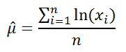
или с помощью формулы
=LN(СРГЕОМ(B16:B215))
, если значения массива размещены в диапазоне
B16:B215
.
Оценку для
σ
(
σ
— параметр распределения, но не
стандартное отклонение
) можно сделать с использованием формулы:
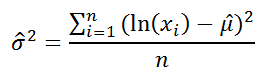
Задачи
Задача1.
Время жизни лазера имеет логнормальное распределение с μ=5 и
σ
=1 час. Какова вероятность того, что лазер проработает >400 часов?
Из определения
интегральной функции распределения
вычислим вероятность того, что лазер проработает меньше 400 часов. Это можно вычислить с помощью формулы (см.
файл примера лист Задачи
):
=ЛОГНОРМ.РАСП(400;5;1;ИСТИНА)=0,16
Тоже значение получим из формулы
=НОРМ.РАСП(LN(400);5;1;ИСТИНА)
Теперь найдем вероятность того, что лазер проработает больше 400 часов:
=1- ЛОГНОРМ.РАСП(400;5;1;ИСТИНА)
Задача2.
Учитывая условие Задачи1, вычислить какой срок жизни будет у 99% лазеров?
Если совокупность лазеров достаточно велика, то можно считать, что вопрос «
Какой срок жизни
x
будет у 99% лазеров?
» эквивалентен вопросу «
Какой срок жизни
x
будет у случайно взятого лазера с вероятностью 99%?
», т.е. вероятность, того что X>
x
равна 99%, где Х – случайная величина, соответствующая времени жизни лазера. Другими словами, после прошествия какого периода времени можно будет с уверенностью 99% сказать, что лазер еще работает. Здесь удобно перейти к дополнительному событию: вероятности того, что лазер сломается. Таким образом, в задаче нам необходимо вычислить значение
х
(время жизни), при котором 1% (1-99%) лазеров сломается, т.е. X<
x
.
Как и в предыдущей задаче, для формулировки условия задачи воспользуемся определением
интегральной функции распределения
: вероятность того, что лазер проработает меньше
x
часов равна 1%. Для вычисления
х
в MS EXCEL 2010 существует функция
ЛОГНОРМ.ОБР()
.
Формула
=ЛОГНОРМ.ОБР(1-99%;5;1)
вернет значение 14,49 часов, т.е. после 14,49 часов с начала работы 99% лазеров будут еще работать.
Примечание
: пользователям более ранних версий MS EXCEL можно посоветовать для расчетов воспользоваться формулами
=EXP(НОРМОБР(1-99%;5;1))
или
=ЛОГНОРМОБР(1-99%;5;1)
.
Задача3.
Учитывая условие Задачи1, вычислить среднее и стандартное отклонение времени жизни лазера.
Для заданных параметров
логнормального распределения
среднее
значение времени жизни лазера
=EXP(5+(1*1)/2)=244,69
часов, а
стандартное отклонение
=КОРЕНЬ((EXP(1*1)-1)*EXP(2*5+1*1))=320,75
часов.
Обратите внимание, что для
логнормального распределения
, как для типичного скошенного распределения,
стандартное отклонение
существенно больше
среднего
.
СОВЕТ
: О других распределениях MS EXCEL можно прочитать в статье
Распределения случайной величины в MS EXCEL
.