by
· Published
May 6, 2021
· Updated
June 16, 2022

Introduction
This blog provides a non-technical look at impulse response functions and forecast error variance decomposition, both integral parts of vector autoregressive models.
If you’re looking to gain a better understanding of these important multivariate time series techniques, you’re in the right place. We cover the basics, including:
- What is structural analysis?
- What are impulse response functions?
- How do we interpret impulse response functions?
- What is forecast error variance decomposition?
- How do we interpret forecast error variance decomposition?
What is structural analysis?
VAR models are widely used in finance and econometrics because they offer a framework for understanding the intertwined relationships of multivariate time series data in a systematic manner.
Reduced-form VAR estimates can be complex, difficult to understand, and generally aren’t insightful on their own. More valuable insights come from structural analysis. In structural analysis, we apply the VAR relationship to understand the dynamic relationship between the variables in our model.
Structural analysis begins with the structural vector autoregression (SVAR). SVAR applies restrictions that allow us to identify the impacts that exogenous shocks have on the variables in the system.
Once the SVAR model is estimated, impulse response functions and forecast error variance decomposition are two of the most important structural analysis tools for examining those impacts.
| Applications of structural analysis after VAR |
|---|
| What impact does monetary policy have on real GDP? |
| How does a shock to income impact consumption paths? |
| Do exchange rate shocks pass through to international currencies? |
Impulse response functions trace the dynamic impact to a system of a “shock” or change to an input. While impulse response functions are used in many fields, they are particularly useful in economics and finance for a number of reasons:
- They are consistent with how we use theoretical economic and finance models. Theoretical economists develop a model, then ask how outcomes change in the face of exogenous changes.
- They can be used to predict the implications of policy changes in a macroeconomic framework.
- They employ structural restrictions which allow us to model our believed theoretical relationships in the economy.
In stationary systems, we expect that the shocks to the system are not persistent and over time the system converges. When the system converges, it may or may not converge to the original state, depending on the restrictions imposed on our structural VAR model.
For example, Blanchard and Quah(1989) famously demonstrated the use of long-run restrictions in a structural VAR to trace the impact of aggregate supply and aggregate demand shocks on output and unemployment. In their model:
- They allow aggregate supply shocks to have lasting effects on output.
- Assume that aggregate demand shocks do not have lasting effects on long-run output.
As a result, when a positive aggregate supply shock occurs, output converges to a higher level than before the shock.
There is a clear modeling procedure to obtaining the impulse response functions:
- Determine appropriate restrictions based on theory and/or previous empirical models.
- Estimate the structural VAR model.
- Predict the impulse response functions for a specified time horizon along with their confidence bands.
- Plot the predicted IRF and their confidence bands.
How do we interpret impulse response functions?
Impulse responses are most often interpreted through grid graphs of the individual responses of each variable to an implemented shock over a specified time horizon.
Let’s look at an example to see how we can interpret these graphs.

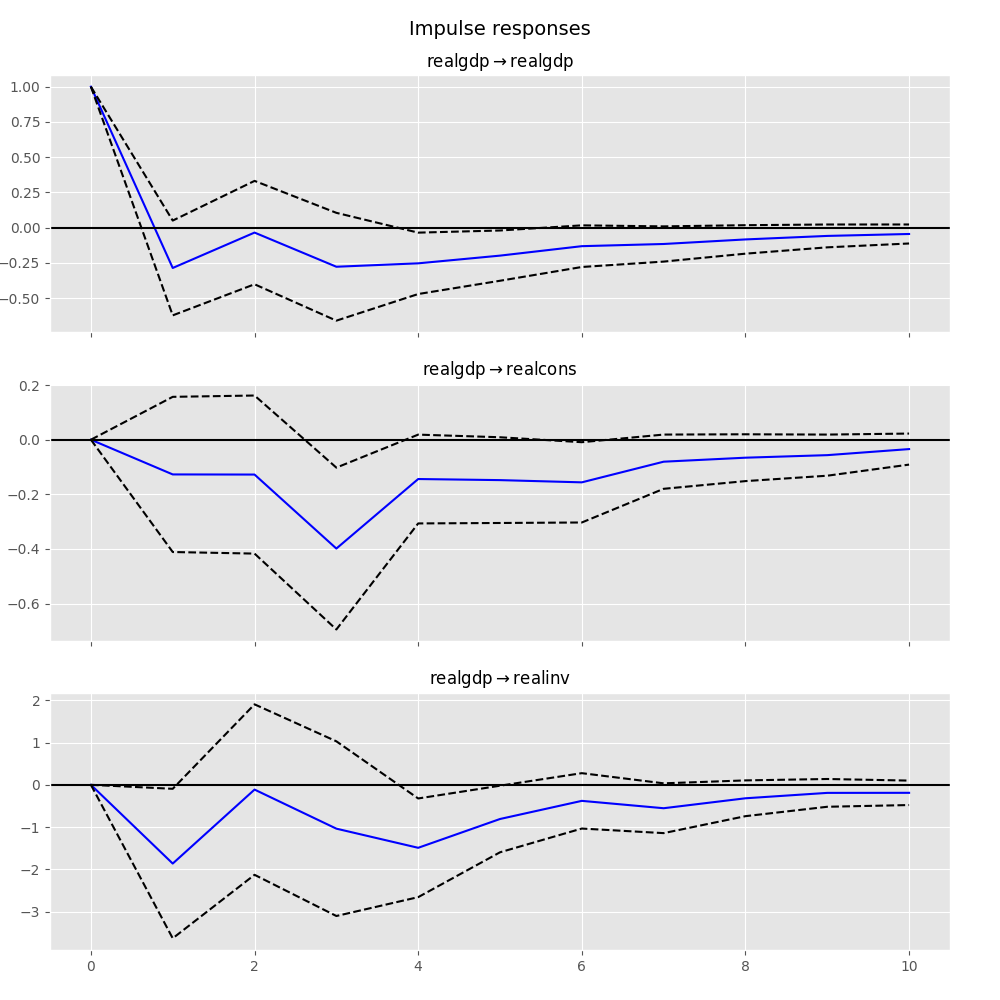
Example: VAR(2) Model of Consumption, Investment, and Income
The graph above shows the impulse response functions for a VAR(2) of income, consumption, and investment. These IRFs show the impact of a one standard deviation shock to income.
In order to estimate the structural VAR, short-run restrictions on the model were employed. These restrictions are such that:
- Income shocks cannot contemporaneously (i.e. immediately) impact investment.
- Consumption shocks cannot contemporaneously impact income or investment.

Let’s look first at the IRF tracing the impact of the shock to income on income itself. In this graph, we see:
- The initial shock to in income in the first period.
- This shock quickly dies as the impact returns to almost zero in the second period.
- A slight increase in income in periods 2-4, with a post-shock peak in period 4.
- The impact converges back to zero after period 4.

The consumption graph shows:
- A quick jump in consumption at the time of the income increase — this is consistent with the economic theory that consumption is a normal good (it increases with increases in income).
- A second spike in consumption occurs around the third period — this is likely a lagging response to the increase in investment.

In the investment response to the income shock, we note that there:
- Is no first-period impact of the income shock on investment. This is by design and results directly from the restrictions implemented in order to estimate the SVAR.
- A short period of positive impact periods 2-4 which converges back to zero.
What is forecast error variance decomposition?
Forecast error variance decomposition (FEVD) is a part of structural analysis which «decomposes» the variance of the forecast error into the contributions from specific exogenous shocks.
Intuitively this is useful because it:
- Demonstrates how important a shock is in explaining the variations of the variables in the model.
- Shows how that importance changes over time. For example, some shocks may not be responsible for variations in the short-run but may cause longer-term fluctuations.
As an example, FEVD may be used to explain how much various shocks, like supply and demand shocks, technology shocks, or monetary policy shocks, contribute to business cycle variations or long-term economic growth.
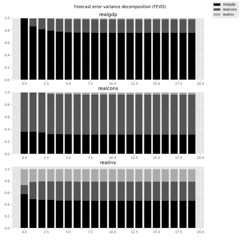
Like impulse response functions, forecast error variance decompositions are generally presented graphically, as either a bar graph or an area graph. At each time period, the graph plots the composition of the error variance across shocks to all the variables.
How do we interpret forecast variance error decompositions (FEVD)?
To understand how we interpret FEVD let’s look at an example VAR(4) model (with a time trend and constant) of inflation, per-capita output, and the Federal Funds rate.

The plot above graphs the FEVD of the Federal Funds rate. This plot, like all FEVD plots:
- Has a Y-range from 0 to 100%.
- Shows the contributions from each individual shock as a portion of the total area (or bar) at any time period.
From this we can tell that:
- In the initial period, approximately 90% of the variation in the Federal Funds rate is from shocks to the Federal Funds rate itself and most of the remaining 10% is from inflation.
- The contribution of per-capita output to the variation in the Federal Funds rate changes fairly rapidly over the first 5 periods and eventually seems to converge at around 40%.
- The contribution of inflation to variations in the Federal Fund rate rises more slowly than that of per-capita output and levels off at roughly 20%.
- The system becomes stable after 15-20 periods.
Conclusion
Today we’ve provided an intuitive look at impulse response functions and forecast error variance decompositions. These two multivariate time series tools are fundamental applications of the structural VAR model.
After today, you should have a better understanding of what these tools are and how to apply them.
Further Reading
- Introduction to the Fundamentals of Time Series Data and Analysis
- Introduction to the Fundamentals of Vector Autoregressive Models
- Introduction to Granger Causality

Eric( Director of Applications and Training at Aptech Systems, Inc. )
Eric has been working to build, distribute, and strengthen the GAUSS universe since 2012. He is an economist skilled in data analysis and software development. He has earned a B.A. and MSc in economics and engineering and has over 18 years of combined industry and academic experience in data analysis and research.

statsmodels.tsa.vector_ar contains methods that are useful
for simultaneously modeling and analyzing multiple time series using
Vector Autoregressions (VAR) and
Vector Error Correction Models (VECM).
VAR(p) processes
We are interested in modeling a (T times K) multivariate time series
(Y), where (T) denotes the number of observations and (K) the
number of variables. One way of estimating relationships between the time series
and their lagged values is the vector autoregression process:
[ begin{align}begin{aligned}Y_t = nu + A_1 Y_{t-1} + ldots + A_p Y_{t-p} + u_t\u_t sim {sf Normal}(0, Sigma_u)end{aligned}end{align} ]
where (A_i) is a (K times K) coefficient matrix.
We follow in large part the methods and notation of Lutkepohl (2005),
which we will not develop here.
Model fitting
Note
The classes referenced below are accessible via the
statsmodels.tsa.api module.
To estimate a VAR model, one must first create the model using an ndarray of
homogeneous or structured dtype. When using a structured or record array, the
class will use the passed variable names. Otherwise they can be passed
explicitly:
# some example data
In [1]: import numpy as np

In [2]: import pandas

In [3]: import statsmodels.api as sm

In [4]: from statsmodels.tsa.api import VAR

In [5]: mdata = sm.datasets.macrodata.load_pandas().data

# prepare the dates index
In [6]: dates = mdata[['year', 'quarter']].astype(int).astype(str)

In [7]: quarterly = dates["year"] + "Q" + dates["quarter"]

In [8]: from statsmodels.tsa.base.datetools import dates_from_str

In [9]: quarterly = dates_from_str(quarterly)

In [10]: mdata = mdata[['realgdp','realcons','realinv']]

In [11]: mdata.index = pandas.DatetimeIndex(quarterly)

In [12]: data = np.log(mdata).diff().dropna()

# make a VAR model
In [13]: model = VAR(data)
Note
The VAR class assumes that the passed time series are
stationary. Non-stationary or trending data can often be transformed to be
stationary by first-differencing or some other method. For direct analysis of
non-stationary time series, a standard stable VAR(p) model is not
appropriate.
To actually do the estimation, call the fit method with the desired lag
order. Or you can have the model select a lag order based on a standard
information criterion (see below):
In [14]: results = model.fit(2)

In [15]: results.summary()
Out[15]:
  Summary of Regression Results
==================================
Model:                         VAR
Method:                        OLS
Date:           Wed, 08, Feb, 2023
Time:                     21:40:34
--------------------------------------------------------------------
No. of Equations:         3.00000    BIC:                   -27.5830
Nobs:                     200.000    HQIC:                  -27.7892
Log likelihood:           1962.57    FPE:                7.42129e-13
AIC:                     -27.9293    Det(Omega_mle):     6.69358e-13
--------------------------------------------------------------------
Results for equation realgdp
==============================================================================
                 coefficient       std. error           t-stat            prob
------------------------------------------------------------------------------
const               0.001527         0.001119            1.365           0.172
L1.realgdp         -0.279435         0.169663           -1.647           0.100
L1.realcons         0.675016         0.131285            5.142           0.000
L1.realinv          0.033219         0.026194            1.268           0.205
L2.realgdp          0.008221         0.173522            0.047           0.962
L2.realcons         0.290458         0.145904            1.991           0.047
L2.realinv         -0.007321         0.025786           -0.284           0.776
==============================================================================

Results for equation realcons
==============================================================================
                 coefficient       std. error           t-stat            prob
------------------------------------------------------------------------------
const               0.005460         0.000969            5.634           0.000
L1.realgdp         -0.100468         0.146924           -0.684           0.494
L1.realcons         0.268640         0.113690            2.363           0.018
L1.realinv          0.025739         0.022683            1.135           0.257
L2.realgdp         -0.123174         0.150267           -0.820           0.412
L2.realcons         0.232499         0.126350            1.840           0.066
L2.realinv          0.023504         0.022330            1.053           0.293
==============================================================================

Results for equation realinv
==============================================================================
                 coefficient       std. error           t-stat            prob
------------------------------------------------------------------------------
const              -0.023903         0.005863           -4.077           0.000
L1.realgdp         -1.970974         0.888892           -2.217           0.027
L1.realcons         4.414162         0.687825            6.418           0.000
L1.realinv          0.225479         0.137234            1.643           0.100
L2.realgdp          0.380786         0.909114            0.419           0.675
L2.realcons         0.800281         0.764416            1.047           0.295
L2.realinv         -0.124079         0.135098           -0.918           0.358
==============================================================================

Correlation matrix of residuals
             realgdp  realcons   realinv
realgdp     1.000000  0.603316  0.750722
realcons    0.603316  1.000000  0.131951
realinv     0.750722  0.131951  1.000000
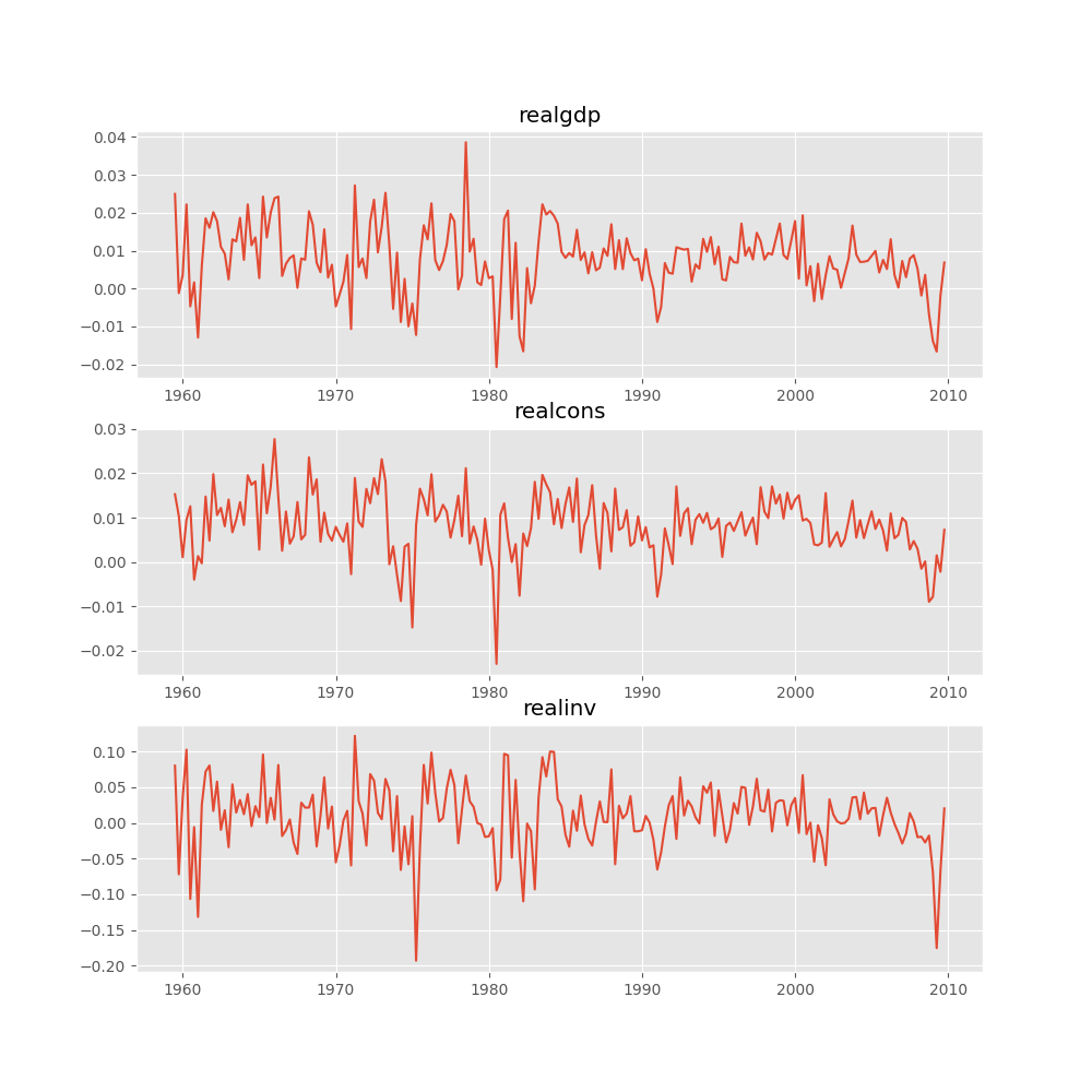
Several ways to visualize the data using matplotlib are available.
Plotting input time series:
In [16]: results.plot()
Out[16]: <Figure size 1000x1000 with 3 Axes>
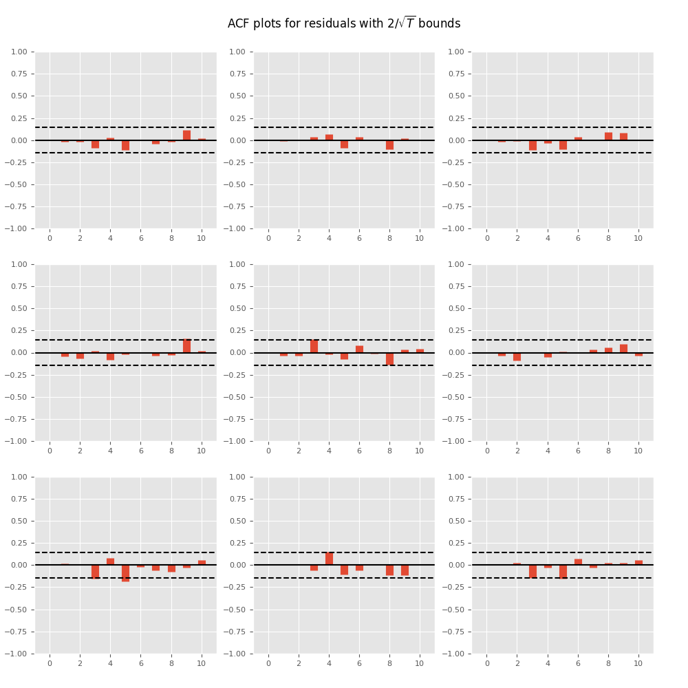
Plotting time series autocorrelation function:
In [17]: results.plot_acorr()
Out[17]: <Figure size 1000x1000 with 9 Axes>
Lag order selection
Choice of lag order can be a difficult problem. Standard analysis employs
likelihood test or information criteria-based order selection. We have
implemented the latter, accessible through the VAR class:
In [18]: model.select_order(15)
Out[18]: <statsmodels.tsa.vector_ar.var_model.LagOrderResults at 0x7f530c6d4ca0>
When calling the fit function, one can pass a maximum number of lags and the
order criterion to use for order selection:
In [19]: results = model.fit(maxlags=15, ic='aic')
Forecasting
The linear predictor is the optimal h-step ahead forecast in terms of
mean-squared error:
[y_t(h) = nu + A_1 y_t(h − 1) + cdots + A_p y_t(h − p)]
We can use the forecast function to produce this forecast. Note that we have
to specify the “initial value” for the forecast:
In [20]: lag_order = results.k_ar

In [21]: results.forecast(data.values[-lag_order:], 5)
Out[21]:
array([[ 0.0062,  0.005 ,  0.0092],
       [ 0.0043,  0.0034, -0.0024],
       [ 0.0042,  0.0071, -0.0119],
       [ 0.0056,  0.0064,  0.0015],
       [ 0.0063,  0.0067,  0.0038]])
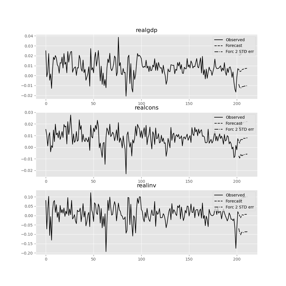
The forecast_interval function will produce the above forecast along with
asymptotic standard errors. These can be visualized using the plot_forecast
function:
In [22]: results.plot_forecast(10)
Out[22]: <Figure size 1000x1000 with 3 Axes>
Class Reference
|
|
Fit VAR(p) process and do lag order selection |
|
|
Class represents a known VAR(p) process |
|
|
Estimate VAR(p) process with fixed number of lags |
Post-estimation Analysis
Several process properties and additional results after
estimation are available for vector autoregressive processes.
|
|
Results class for choosing a model’s lag order. |
Impulse Response Analysis
Impulse responses are of interest in econometric studies: they are the
estimated responses to a unit impulse in one of the variables. They are computed
in practice using the MA((infty)) representation of the VAR(p) process:
[Y_t = mu + sum_{i=0}^infty Phi_i u_{t-i}]
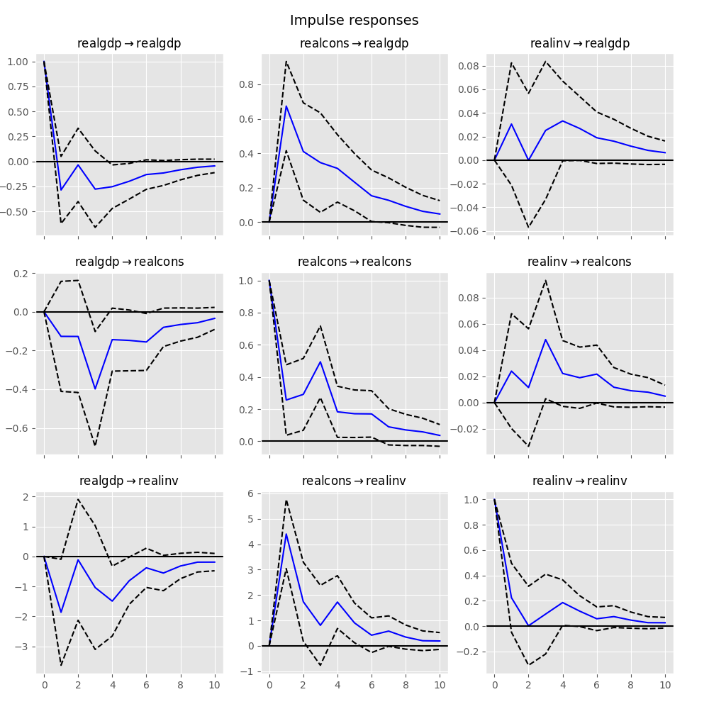
We can perform an impulse response analysis by calling the irf function on a
VARResults object:
In [23]: irf = results.irf(10)
These can be visualized using the plot function, in either orthogonalized or
non-orthogonalized form. Asymptotic standard errors are plotted by default at
the 95% significance level, which can be modified by the user.
Note
Orthogonalization is done using the Cholesky decomposition of the estimated
error covariance matrix (hat Sigma_u) and hence interpretations may
change depending on variable ordering.
In [24]: irf.plot(orth=False)
Out[24]: <Figure size 1000x1000 with 9 Axes>
Note the plot function is flexible and can plot only variables of interest if
so desired:
In [25]: irf.plot(impulse='realgdp')
Out[25]: <Figure size 1000x1000 with 3 Axes>
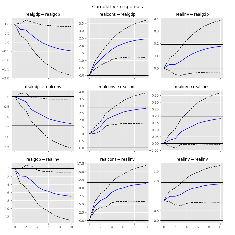
The cumulative effects (Psi_n = sum_{i=0}^n Phi_i) can be plotted with
the long run effects as follows:
In [26]: irf.plot_cum_effects(orth=False)
Out[26]: <Figure size 1000x1000 with 9 Axes>
|
|
Impulse response analysis class. |
Forecast Error Variance Decomposition (FEVD)
Forecast errors of component j on k in an i-step ahead forecast can be
decomposed using the orthogonalized impulse responses (Theta_i):
[ begin{align}begin{aligned}omega_{jk, i} = sum_{i=0}^{h-1} (e_j^prime Theta_i e_k)^2 / mathrm{MSE}_j(h)\mathrm{MSE}_j(h) = sum_{i=0}^{h-1} e_j^prime Phi_i Sigma_u Phi_i^prime e_jend{aligned}end{align} ]
These are computed via the fevd function up through a total number of steps ahead:
In [27]: fevd = results.fevd(5)

In [28]: fevd.summary()
FEVD for realgdp
      realgdp  realcons   realinv
0    1.000000  0.000000  0.000000
1    0.864889  0.129253  0.005858
2    0.816725  0.177898  0.005378
3    0.793647  0.197590  0.008763
4    0.777279  0.208127  0.014594

FEVD for realcons
      realgdp  realcons   realinv
0    0.359877  0.640123  0.000000
1    0.358767  0.635420  0.005813
2    0.348044  0.645138  0.006817
3    0.319913  0.653609  0.026478
4    0.317407  0.652180  0.030414

FEVD for realinv
      realgdp  realcons   realinv
0    0.577021  0.152783  0.270196
1    0.488158  0.293622  0.218220
2    0.478727  0.314398  0.206874
3    0.477182  0.315564  0.207254
4    0.466741  0.324135  0.209124
They can also be visualized through the returned FEVD object:
In [29]: results.fevd(20).plot()
Out[29]: <Figure size 1000x1000 with 3 Axes>
|
|
Compute and plot Forecast error variance decomposition and asymptotic standard errors |
Statistical tests
A number of different methods are provided to carry out hypothesis tests about
the model results and also the validity of the model assumptions (normality,
whiteness / “iid-ness” of errors, etc.).
Granger causality
One is often interested in whether a variable or group of variables is “causal”
for another variable, for some definition of “causal”. In the context of VAR
models, one can say that a set of variables are Granger-causal within one of the
VAR equations. We will not detail the mathematics or definition of Granger
causality, but leave it to the reader. The VARResults object has the
test_causality method for performing either a Wald ((chi^2)) test or an
F-test.
In [30]: results.test_causality('realgdp', ['realinv', 'realcons'], kind='f')
Out[30]: <statsmodels.tsa.vector_ar.hypothesis_test_results.CausalityTestResults at 0x7f530be2c7f0>
Normality
As pointed out in the beginning of this document, the white noise component
(u_t) is assumed to be normally distributed. While this assumption
is not required for parameter estimates to be consistent or asymptotically
normal, results are generally more reliable in finite samples when residuals
are Gaussian white noise. To test whether this assumption is consistent with
a data set, VARResults offers the test_normality method.
In [31]: results.test_normality()
Out[31]: <statsmodels.tsa.vector_ar.hypothesis_test_results.NormalityTestResults at 0x7f530be2ded0>
Whiteness of residuals
To test the whiteness of the estimation residuals (this means absence of
significant residual autocorrelations) one can use the test_whiteness
method of VARResults.
Structural Vector Autoregressions
There are a matching set of classes that handle some types of Structural VAR models.
|
|
Fit VAR and then estimate structural components of A and B, defined: |
|
|
Class represents a known SVAR(p) process |
|
|
Estimate VAR(p) process with fixed number of lags |
Vector Error Correction Models (VECM)
Vector Error Correction Models are used to study short-run deviations from
one or more permanent stochastic trends (unit roots). A VECM models the
difference of a vector of time series by imposing structure that is implied
by the assumed number of stochastic trends. VECM is used to
specify and estimate these models.
A VECM((k_{ar}-1)) has the following form
[Delta y_t = Pi y_{t-1} + Gamma_1 Delta y_{t-1} + ldots
+ Gamma_{k_{ar}-1} Delta y_{t-k_{ar}+1} + u_t]
where
[Pi = alpha beta’]
as described in chapter 7 of [1].
A VECM((k_{ar} — 1)) with deterministic terms has the form
[begin{split}Delta y_t = alpha begin{pmatrix}beta’ & eta’end{pmatrix} begin{pmatrix}y_{t-1} \
D^{co}_{t-1}end{pmatrix} + Gamma_1 Delta y_{t-1} + dots + Gamma_{k_{ar}-1} Delta y_{t-k_{ar}+1} + C D_t + u_t.end{split}]
In (D^{co}_{t-1}) we have the deterministic terms which are inside
the cointegration relation (or restricted to the cointegration relation).
(eta) is the corresponding estimator. To pass a deterministic term
inside the cointegration relation, we can use the exog_coint argument.
For the two special cases of an intercept and a linear trend there exists
a simpler way to declare these terms: we can pass "ci" and "li"
respectively to the deterministic argument. So for an intercept inside
the cointegration relation we can either pass "ci" as deterministic
or np.ones(len(data)) as exog_coint if data is passed as the
endog argument. This ensures that (D_{t-1}^{co} = 1) for all
(t).
We can also use deterministic terms outside the cointegration relation.
These are defined in (D_t) in the formula above with the
corresponding estimators in the matrix (C). We specify such terms by
passing them to the exog argument. For an intercept and/or linear trend
we again have the possibility to use deterministic alternatively. For
an intercept we pass "co" and for a linear trend we pass "lo" where
the o stands for outside.
The following table shows the five cases considered in [2]. The last
column indicates which string to pass to the deterministic argument for
each of these cases.
|
Case |
Intercept |
Slope of the linear trend |
deterministic |
|---|---|---|---|
|
I |
0 |
0 |
|
|
II |
(- alpha beta^T mu) |
0 |
|
|
III |
(neq 0) |
0 |
|
|
IV |
(neq 0) |
(- alpha beta^T gamma) |
|
|
V |
(neq 0) |
(neq 0) |
|
|
|
Class representing a Vector Error Correction Model (VECM). |
|
|
Johansen cointegration test of the cointegration rank of a VECM |
|
|
Results class for Johansen’s cointegration test |
|
|
Compute lag order selections based on each of the available information criteria. |
|
|
Calculate the cointegration rank of a VECM. |
|
|
Class for holding estimation related results of a vector error correction model (VECM). |
|
|
A class for holding the results from testing the cointegration rank. |
References
Generate forecast error variance decomposition (FEVD) of state-space model
Syntax
Description
The fevd function returns the forecast error variance decomposition (FEVD) of the measurement variables in a state-space model attributable to component-wise shocks to each state disturbance. The FEVD provides information about the relative importance of each state disturbance in affecting the forecast error variance of all measurement variables in the system. Other state-space model tools to characterize the dynamics of a specified system include the following:
-
The impulse response function (IRF), computed by
irfand plotted byirfplot, traces the effects of a shock to a state disturbance on the state and measurement variables in the system. -
Model-implied temporal correlations, computed by
corrfor a standard state-space model, measure the association between current and lagged state or measurement variables, as prescribed by the form of the model.
Fully Specified State-Space Model
example
Decomposition = fevd(Mdl)Decomposition of the fully specified state-space model Mdl.
example
Decomposition = fevd(Mdl,Name,Value)'NumPeriods',10 specifies estimating the FEVD for periods 1 through 10.
Partially Specified State-Space Model and Confidence Interval Estimation
example
Decomposition = fevd(___,'Params',estParams)Mdl. estParams specifies estimates of all unknown parameters in the model, using any of the input argument combinations in the previous syntaxes.
example
[ also returns the lower and upper 95% Monte Carlo confidence bounds Decomposition,Lower,Upper] = fevd(___,'Params',estParams,'EstParamCov',EstParamCov)Lower and Upper of each measurement variable FEVD. EstParamCov specifies the estimated covariance matrix of the parameter estimates, as returned by the estimate function, and is required for confidence interval estimation.
Examples
collapse all
FEVD of Measurement Variables
Compute the model-implied FEVD of two state-space models: one with measurement error and one without measurement error.
Model Without Measurement Error
Explicitly create the state-space model without measurement error
x1,t=x1,t-1+0.2u1,tx2,t=x1,t-1+0.3×2,t-1+u2,ty1,t=x1,ty2,t=x1,t+x2,t.
A = [1 0; 1 0.3];
B = [0.2 0; 0 1];
C = [1 0; 1 1];
Mdl1 = ssm(A,B,C,'StateType',[2 2])
Mdl1 =
State-space model type: ssm

State vector length: 2
Observation vector length: 2
State disturbance vector length: 2
Observation innovation vector length: 0
Sample size supported by model: Unlimited

State variables: x1, x2,...
State disturbances: u1, u2,...
Observation series: y1, y2,...
Observation innovations: e1, e2,...

State equations:
x1(t) = x1(t-1) + (0.20)u1(t)
x2(t) = x1(t-1) + (0.30)x2(t-1) + u2(t)

Observation equations:
y1(t) = x1(t)
y2(t) = x1(t) + x2(t)

Initial state distribution:

Initial state means
 x1  x2
  0   0

Initial state covariance matrix
     x1     x2
 x1  1e+07  0
 x2  0      1e+07

State types
    x1       x2
 Diffuse  Diffuse
Mdl1 is an ssm model object. Because all parameters have known values, the object is fully specified.
Compute the 20-period FEVD of the measurement variables.
Decomposition1 = fevd(Mdl1);
size(Decomposition1)
Decomposition is a 20-by-2-by-2 array representing the 20-period FEVD of the two measurement variables. Display Decomposition(5,1,2).
In this case, 44.29% of the volatility of y2,t is attributed to the shock applied to u1,t-5.
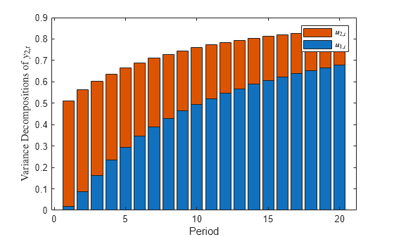
Plot the FEVD of y2,t for each state disturbance.
bar(Decomposition1(:,:,2),'stacked')
xlabel('Period')
ylabel('Variance decompositions of $y_{2,t}$','Interpreter','latex')
legend('$u_{1,t}$','$u_{2,t}$','Interpreter','latex')
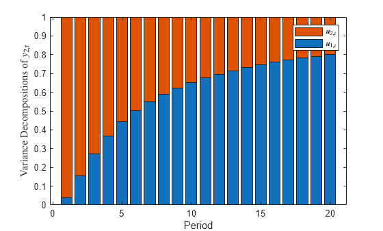
Because the state-space model is free of measurement error (D = 0), the variance decompositions of each period sum to 1. The volatility attributable to u1,t increases with each period.
Model with Measurement Error
Explicitly create the state-space model
x1,t=x1,t-1+0.2u1,tx2,t=x1,t-1+0.3×2,t-1+u2,ty1,t=x1,t+ε1,ty2,t=x1,t+x2,t+ε2,t.
D = eye(2);
Mdl2 = ssm(A,B,C,D,'StateType',[2 2])
Mdl2 =
State-space model type: ssm

State vector length: 2
Observation vector length: 2
State disturbance vector length: 2
Observation innovation vector length: 2
Sample size supported by model: Unlimited

State variables: x1, x2,...
State disturbances: u1, u2,...
Observation series: y1, y2,...
Observation innovations: e1, e2,...

State equations:
x1(t) = x1(t-1) + (0.20)u1(t)
x2(t) = x1(t-1) + (0.30)x2(t-1) + u2(t)

Observation equations:
y1(t) = x1(t) + e1(t)
y2(t) = x1(t) + x2(t) + e2(t)

Initial state distribution:

Initial state means
 x1  x2
  0   0

Initial state covariance matrix
     x1     x2
 x1  1e+07  0
 x2  0      1e+07

State types
    x1       x2
 Diffuse  Diffuse
Compute the 20-period FEVD of the measurement variables.
Decomposition2 = fevd(Mdl2);
Plot the FEVD of y2,t for each state disturbance.
bar(Decomposition2(:,:,2),'stacked')
xlabel('Period')
ylabel('Variance decompositions of $y_{2,t}$','Interpreter','latex')
legend('$u_{1,t}$','$u_{2,t}$','Interpreter','latex')
Because the model contains measurement error, the variance proportions do not sum to 1 during each period.
Specify Number of Periods
Explicitly create the multivariate diffuse state-space model
x1,t=x1,t-1+0.2u1,tx2,t=x1,t-1+0.3×2,t-1+u2,ty1,t=x1,ty2,t=x1,t+x2,t.
A = [1 0; 1 0.3];
B = [0.2 0; 0 1];
C = [1 0; 1 1];
Mdl = dssm(A,B,C,'StateType',[2 2])
Mdl =
State-space model type: dssm

State vector length: 2
Observation vector length: 2
State disturbance vector length: 2
Observation innovation vector length: 0
Sample size supported by model: Unlimited

State variables: x1, x2,...
State disturbances: u1, u2,...
Observation series: y1, y2,...
Observation innovations: e1, e2,...

State equations:
x1(t) = x1(t-1) + (0.20)u1(t)
x2(t) = x1(t-1) + (0.30)x2(t-1) + u2(t)

Observation equations:
y1(t) = x1(t)
y2(t) = x1(t) + x2(t)

Initial state distribution:

Initial state means
 x1  x2
  0   0

Initial state covariance matrix
     x1   x2
 x1  Inf  0
 x2  0    Inf

State types
    x1       x2
 Diffuse  Diffuse
Mdl is a dssm model object.
Compute the 50-period FEVD of the measurement variables.
Decomposition = fevd(Mdl,'NumPeriods',50);
size(Decomposition)
Plot the FEVD of y2,t for each state disturbance.
bar(Decomposition(:,:,2),'stacked')
xlabel('Period')
ylabel('Variance decompositions of $y_{2,t}$','Interpreter','latex')
legend('$u_{1,t}$','$u_{2,t}$','Interpreter','latex')
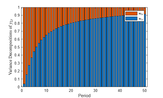
The contribution of u1,t to the volatility of y2,t approaches 90%.
FEVD of Estimated Model
Simulate data from a known model, fit the data to a state-space model, and then estimate the FEVD of the measurement variables.
Consider the time series decomposition yt=τt+ct, where τt is a random walk with drift representing the trend component, and ct is an AR(1) model representing the cycle component.
τt=3+τt-1+u1,tct=0.5ct-1+2u2,t.
The model in state-space notation is
xt=[τtdtct]=[130010000.5][τt-1dt-1ct-1]+[100002][u1,tu2,t]yt=[101]xt,
where dt is a dummy state representing the drift parameter, which is 1 for all t.
Simulate 500 observations from the true model.
rng(1); % For reproducibility
ADGP = [1 3 0; 0 1 0; 0 0 0.5];
BDGP = [1 0; 0 0; 0 2];
CDGP = [1 0 1];
DGP = ssm(ADGP,BDGP,CDGP,'StateType',[2 1 0]);
y = simulate(DGP,500);
Assume that the drift constant, disturbance variances, and AR coefficient are unknown. Explicitly create a state-space model template for estimation that represents the model by replacing the unknown parameters in the model with NaN.
A = [1 NaN 0; 0 1 0; 0 0 NaN];
B = [NaN 0; 0 0; 0 NaN];
C = CDGP;
Mdl = ssm(A,B,C,'StateType',[2 1 0]);
Fit the model template to the data. Specify a set of positive, random standard Gaussian starting values for the four model parameters. Return the estimated model and vector of parameter estimates.
[EstMdl,estParams] = estimate(Mdl,y,abs(randn(4,1)),'Display','off')
EstMdl =
State-space model type: ssm

State vector length: 3
Observation vector length: 1
State disturbance vector length: 2
Observation innovation vector length: 0
Sample size supported by model: Unlimited

State variables: x1, x2,...
State disturbances: u1, u2,...
Observation series: y1, y2,...
Observation innovations: e1, e2,...

State equations:
x1(t) = x1(t-1) + (2.91)x2(t-1) + (0.92)u1(t)
x2(t) = x2(t-1)
x3(t) = (0.52)x3(t-1) + (2.13)u2(t)

Observation equation:
y1(t) = x1(t) + x3(t)

Initial state distribution:

Initial state means
 x1  x2  x3
  0   1   0

Initial state covariance matrix
     x1        x2  x3
 x1  1.00e+07   0   0
 x2   0         0   0
 x3   0         0  6.20

State types
    x1       x2         x3
 Diffuse  Constant  Stationary
estParams = 4×1

    2.9115
    0.5189
    0.9200
    2.1278
EstMdl is a fully specified ssm model object. Model estimates are close to their true values.
Compute and plot the FEVD of the measurement variable. Specify the model template Mdl and the vector of estimated parameters estParams.
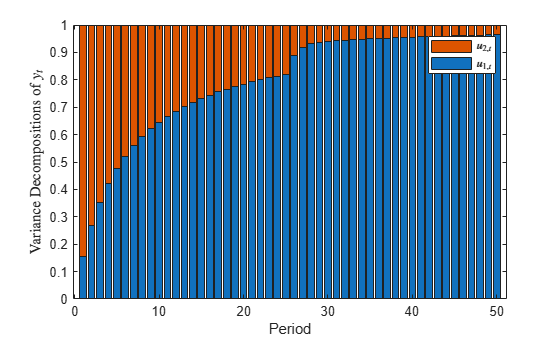
Decomposition = fevd(Mdl,'Params',estParams);

bar(Decomposition,'stacked')
xlabel('Period')
ylabel('Variance decompositions of $y_{t}$','Interpreter','latex')
legend('$u_{1,t}$','$u_{2,t}$','Interpreter','latex')

Noise in the cyclical component dominates the volatility of the measurement variable in low lags, with increasing contribution from the trend component noise as the lag increases.
Time-Varying FEVD
Simulate data from a time-varying state-space model, fit a model to the data, and then estimate the time-varying FEVD of the measurement variable.
Consider the time series decomposition yt=τt+ct, where τt is a random walk with drift representing the trend component, and ct is an AR(1) model representing the cyclical component. Suppose that the cyclical component changes during period 26 over a 50-period time span.
τt=1+τt-1+u1,tct={0.5ct+2u2,t;t<26-0.2ct+0.5u2,t;t≥26.
The function timeVariantTrendCycleParamMap.m, stored in mlr/examples/econ/main, specifies the model structure. mlr is the value of matlabroot.
type timeVariantTrendCycleParamMap.m
% Copyright 2021 The MathWorks, Inc.

function [A,B,C,D,Mean0,Cov0,StateType] = timeVariantTrendCycleParamMap(params)
% Time-varying state-space model parameter mapping function example. This
% function maps the vector params to the state-space matrices (A, B, C, and
% D). The measurement equation is a times series decomposed into trend and
% cyclical components, with a structural break in the cycle during period
% 26.
%
% The trend component is tau_t = drift + tau_{t-1} + s_1u1_t.
%
% The cyclical component is:
%     * c_t = phi_1*c_{t-1} + s_2*u2_t; t = 1 through 25
%     * c_t = phi_2*c_{t-1} + s_3*u2_t; t = 11 through 26.
%
% The measurement equation is y_t = tau_t + c_t.
    A1 = {[1 params(1) 0; 0 1 0; 0 0 params(2)]};
    A2 = {[1 params(1) 0; 0 1 0; 0 0 params(3)]};
    varu1 = exp(params(4));  % Positive variance constraints
    varu21 = exp(params(5));
    varu22 = exp(params(6));
    B1 = {[sqrt(varu1) 0; 0 0; 0 sqrt(varu21)]};
    B2 = {[sqrt(varu1) 0; 0 0; 0 sqrt(varu22)]};
    C = [1 0 1];
    D = 0;
    sc = 25;
    A = [repmat(A1,sc,1); repmat(A2,sc,1)];
    B = [repmat(B1,sc,1); repmat(B2,sc,1)];
    Mean0 = [];
    Cov0 = [];
    StateType = [2 1 0];
end
Implicitly create a partially specified state-space model representing the data generating process (DGP).
ParamMap = @timeVariantTrendCycleParamMap;
DGP = ssm(ParamMap);
Simulate 50 observations from the DGP. Because DGP is partially specified, pass the true parameter values to simulate by using the 'Params' name-value argument.
rng(5) % For reproducibility
trueParams = [1 0.5 -0.2 2*log(1) 2*log(2) 2*log(0.5)]; % Transform variances for parameter map
y = simulate(DGP,50,'Params',trueParams);
y is a 50-by-1 vector of simulated measurements yt from the DGP.
Because DGP is a partially specified, implicit model object, its parameters are unknown. Therefore, it can serve as a model template for estimation.
Fit the model to the simulated data. Specify random standard Gaussian draws for the initial parameter values, and turn off the estimation display. Return the parameter estimates.
[~,estParams] = estimate(DGP,y,randn(1,6),'Display','off')
estParams = 1×6

    0.8510    0.0118    0.6309   -0.3227    1.3778   -0.2200
estParams is a 1-by-6 vector of parameter estimates. The output argument list of the parameter mapping function determines the order of the estimates.
Estimate the FEVD of the measurement variable by supplying DGP (not the estimated model) and the estimated parameters using the 'Params' name-value argument.
Decomposition = fevd(DGP,'Params',estParams,'NumPeriods',50);

bar(Decomposition,'stacked')
xlabel('Period')
ylabel('Variance decompositions of $y_{t}$','Interpreter','latex')
legend('$u_{1,t}$','$u_{2,t}$','Interpreter','latex')
The FEVD jumps at period 26, when the structural break occurs.
Estimate FEVD Confidence Bounds
Simulate data from a known model, fit the data to a state-space model, and then estimate the FEVD of the measurement variables with 90% Monte Carlo confidence bounds.
Consider the time series decomposition yt=τt+ct, where τt is a random walk with drift representing the trend component, and ct is an AR(1) model representing the cycle component.
τt=3+τt-1+u1,tct=0.5ct-1+2u2,t.
The model in state-space notation is
xt=[τtdtct]=[130010000.5][τt-1dt-1ct-1]+[100002][u1,tu2,t]yt=[101]xt,
where dt is a dummy state representing the drift parameter, which is 1 for all t.
Simulate 500 observations from the true model.
rng(1); % For reproducibility
ADGP = [1 3 0; 0 1 0; 0 0 0.5];
BDGP = [1 0; 0 0; 0 2];
CDGP = [1 0 1];
DGP = ssm(ADGP,BDGP,CDGP,'StateType',[2 1 0]);
y = simulate(DGP,500);
Assume that the drift constant, disturbance variances, and AR coefficient are unknown. Explicitly create a state-space model template for estimation that represents the model by replacing the unknown parameters in the model with NaN.
A = [1 NaN 0; 0 1 0; 0 0 NaN];
B = [NaN 0; 0 0; 0 NaN];
C = CDGP;
Mdl = ssm(A,B,C,'StateType',[2 1 0]);
Fit the model template to the data. Specify a set of positive, random standard Gaussian starting values for the four model parameters, and turn off the estimation display. Return the estimated model and vector of parameter estimates and their estimated covariance matrix.
[EstMdl,estParams,EstParamCov] = estimate(Mdl,y,abs(randn(4,1)),'Display','off');
EstMdl is a fully specified ssm model object. Model estimates are close to their true values.
Compute the FEVD of the measurement variable with period-wise 90% Monte Carlo confidence bounds. Specify the model template Mdl, vector of estimated parameters estParams, and their estimated covariance matrix EstParamCov.
[Decomposition,Lower,Upper] = fevd(Mdl,'Params',estParams,'EstParamCov',EstParamCov,...
    'Confidence',0.9);
Plot the proportion of volatility of yt attributable to u1,t with corresponding 90% confidence bounds.
plot(Decomposition(:,1),'r-o')
hold on
plot([Lower(:,1) Upper(:,1)],'b-o')
hold off
xlabel('Period')
ylabel('Proportion of volatility')
title('Volatility Attributable to $u_{1,t}$','Interpreter','latex')
legend('Proportion','90% confidence bounds')
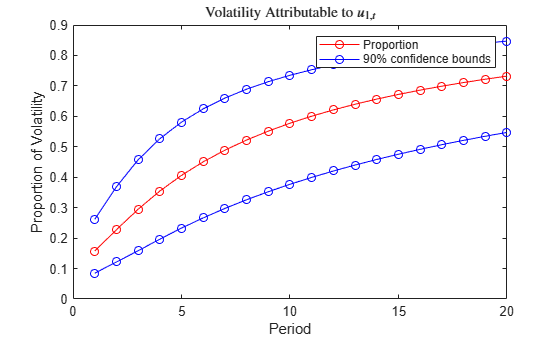
The confidence bounds are initially relatively tight, but widen as the lag and volatility increase.
Input Arguments
collapse all
State-space model, specified as an ssm model object returned by ssm or its estimate function, or a dssm model object returned by dssm or its estimate function.
If Mdl is partially specified (that is, it contains unknown parameters), specify estimates of the unknown parameters by using the 'Params' name-value argument. Otherwise, fevd issues an error.
fevd issues an error when Mdl is a dimension-varying model, which is a time-varying model containing at least one variable that changes dimension during the sampling period (for example, a state variable drops out of the model).
Tip
If Mdl is fully specified, you cannot estimate confidence bounds. To estimate confidence bounds:
-
Create a partially specified state-space model template for estimation
Mdl. -
Estimate the model by using the
estimatefunction and data. Return the estimated parametersestParamsand estimated parameter covariance matrixEstParamCov. -
Pass the model template for estimation
Mdltofevd, and specify the parameter estimates and covariance matrix by using the'Params'and'EstParamCov'name-value arguments. -
For the
fevdfunction, return the appropriate output arguments for lower and upper confidence bounds.
Name-Value Arguments
Specify optional pairs of arguments as
Name1=Value1,...,NameN=ValueN, where Name is
the argument name and Value is the corresponding value.
Name-value arguments must appear after other arguments, but the order of the
pairs does not matter.
Before R2021a, use commas to separate each name and value, and enclose
Name in quotes.
Example: 'NumPeriods',10 estimating the FEVD for specifies estimating the FEVD for periods 1 through 10.
FEVD Options
collapse all
NumPeriods — Number of periods
20 (default) | positive integer
Number of periods for which fevd computes the FEVD, specified as a positive integer. Periods in the FEVD start at time 1 and end at time NumPeriods.
Example:
'NumPeriods',10 specifies the inclusion of 10 consecutive time points in the FEVD, starting at time 1 and ending at time 10.
Data Types: double
Estimates of the unknown parameters in the partially specified state-space model Mdl, specified as a numeric vector.
If Mdl is partially specified (contains unknown parameters specified by NaNs), you must specify Params. The estimate function returns parameter estimates of Mdl in the appropriate form. However, you can supply custom estimates by arranging the elements of Params as follows:
-
If
Mdlis an explicitly created model (Mdl.ParamMapis empty[]), arrange the elements ofParamsto correspond to hits of a column-wise search ofNaNs in the state-space model coefficient matrices, initial state mean vector, and covariance matrix.-
If
Mdlis time invariant, the order isA,B,C,D,Mean0, andCov0. -
If
Mdlis time varying, the order isA{1}throughA{end},B{1}throughB{end},C{1}throughC{end},D{1}throughD{end},Mean0, andCov0.
-
-
If
Mdlis an implicitly created model (Mdl.ParamMapis a function handle), the first input argument of the parameter-to-matrix mapping function determines the order of the elements ofParams.
If Mdl is fully specified, fevd ignores Params.
Example: Consider the state-space model Mdl with A = B = [NaN 0; 0 NaN] , C = [1; 1], D = 0, and initial state means of 0 with covariance eye(2). Mdl is partially specified and explicitly created. Because the model parameters contain a total of four NaNs, Params must be a 4-by-1 vector, where Params(1) is the estimate of A(1,1), Params(2) is the estimate of A(2,2), Params(3) is the estimate of B(1,1), and Params(4) is the estimate of B(2,2).
Data Types: double
Confidence Bound Estimation Options
collapse all
Estimated covariance matrix of unknown parameters in the partially specified state-space model Mdl, specified as a positive semidefinite numeric matrix.
estimate returns the estimated parameter covariance matrix of Mdl in the appropriate form. However, you can supply custom estimates by setting EstParamCov( to the estimated covariance of the estimated parameters i,j)Params( and i)Params(, regardless of whether j)Mdl is time invariant or time varying.
If Mdl is fully specified, fevd ignores EstParamCov.
By default, fevd does not estimate confidence bounds.
Data Types: double
Number of Monte Carlo sample paths (trials) to generate to estimate confidence bounds, specified as a positive integer.
Example: 'NumPaths',5000
Data Types: double
Confidence level for the confidence bounds, specified as a numeric scalar in the interval [0,1].
For each period, randomly drawn confidence intervals cover the true response 100*Confidence% of the time.
The default value is 0.95, which implies that the confidence bounds represent 95% confidence intervals.
Example: Confidence=0.9 specifies 90% confidence
intervals.
Data Types: double
Output Arguments
collapse all
Decomposition — FEVD
numeric array
FEVD of the measurement variables yt, returned as a NumPeriods-by-k-by-n numeric array.
Decomposition( is the FEVD of measurement variable t,i,j)jtitNumPeriods, ij
Lower — Pointwise lower confidence bounds of FEVD
numeric array
Pointwise lower confidence bounds of the FEVD of the measurement variables, returned as a NumPeriods-by-k-by-n numeric array.
Lower( is the lower bound of the t,i,j)100*Confidence% percentile interval on the true FEVD of measurement variable jti
Upper — Pointwise upper confidence bounds of FEVD
numeric array
Pointwise upper confidence bounds of the FEVD of the measurement variables, returned as a NumPeriods-by-k-by-n numeric array.
Upper( is the upper confidence bound corresponding to the lower confidence bound t,i,j)Lower(.t,i,j)
More About
collapse all
Forecast Error Variance Decomposition
The forecast error variance decomposition (FEVD) of a state-space model measures the volatility in each measurement variable yt as a result of a unit impulse to each state disturbance ut at period 1. The FEVD tracks the volatility as the impulses propagate the system for each period t ≥ 1. The FEVD provides information about the relative importance of each state disturbance in affecting the forecast error variance of all measurement variables in the system.
Consider the time-invariant state-space model at time t
and consider unit shocks to all state disturbances ut during period t – s, where s < t.
The state equation, expressed as a function of ut – s is xt=As+1xt−s−1+∑i=0sAiBut−i. The corresponding measurement equation is
Therefore, the total volatility of yt, attributed to shocks from periods t – s through t, is
This result implies that noise in both the transition and measurement equations contributes to the forecast error variance.
The volatility attributed to state disturbance j
uj,t is
where:
-
Ik(j) is a k-by-k
selection matrix, a matrix of zeros except for the value 1 in element (j,j). -
Vs=∑j=1kVsj+DD′
As a result, the s-step ahead forecast error variance of yi,t, attributable to a unit shock to uj,t, is
If D is zero, the FEVD of a measurement variable at period t sums to one (in other words, the sum of each row is one). Otherwise, the FEVD of a measurement variable at period t does not necessarily sum to one; the remaining portion is attributable to DD‘.
The FEVD of a time-varying, dimension-invariant state-space model is also time varying. In this case, fevd always applies the unit shock during period 1. For an s-period-ahead FEVD, the measurement equation is
The total volatility of ys is
As with time-invariant models, the s-period-ahead volatility attributed to state disturbance j shocked during period 1 uj,1 is
As a result, the s-step-ahead forecast error variance of yi,s, attributable to a unit shock to uj,1, is
Because time-invariant and time-varying FEVDs do not include initial state distribution terms, the formulas apply to standard and diffuse state-space models.
Algorithms
-
If you do not supply the
EstParamCovname-value argument, confidence bounds of each period overlap. -
fevduses Monte Carlo simulation to compute confidence intervals.-
fevdrandomly drawsNumPathsvariates from the asymptotic sampling distribution of the unknown parameters inMdl, which is Np(Params,EstParamCov), where p is the number of unknown parameters. -
For each randomly drawn parameter set j,
fevddoes the following:-
Create a state-space model that is equal to
Mdl, but substitute in parameter set j. -
Compute the random FEVD of the resulting model γj(t), where t = 1 through
NumPaths.
-
-
For each time t, the lower bound of the confidence interval is the
(1 –quantile of the simulated FEVD at period tc)/2
γ(t), wherecConfidence. Similarly, the upper bound of the confidence interval at time t is the(1 –upper quantile of γ(t).c)/2
-
Version History
Introduced in R2021a

|
2.1. UNRESTRICTED VECTOR AUTOREGRESSIONS |
29 |
The e ect on q1t at time k of a one standard deviation orthogonalized innovation in η1 at time 0, is b11,k. Similarly, the e ect on q2k is b21,k. Graphing the transformed moving-average coe cients is an e cient method to examine the impulse responses.
You may also want to calculate standard error bands for the impulse responses. You can do this using the following parametric bootstrap procedure.5 Let T be the number of time-series observations you have
and let a ‘tilde’ denote pseudo values generated by the computer, then (12) ‘tilde’
ˆ
1. Take T + M independent draws from the N(0, Σ) to form the vector series {²˜t}.
2. Set startup values of qt at their mean values of 0 then recursively generate the sequence {q˜t} of length T + M according to (2.1)
using the estimated Aj matrices.
3. Drop the Þrst M observations to eliminate dependence on starting values. Estimate the simulated VAR. Call the estimated coe —
˜
cients Aj.
˜˜ ˜−1˜
4.Form the matrices Bj = CjΛ S. You now have one realization (13) of the parametric bootstrap distribution of the impulse response function.
5.Repeat the process say 5000 times. The collection of observations
˜
on the Bj forms the bootstrap distribution. Take the standard deviation of the bootstrap distribution as an estimate of the standard error.
In (2.7), you have decomposed q1t into orthogonal components. The innovation η1t is attributed to q1t and the innovation η2t is attributed
5The bootstrap is a resampling scheme done by computer to estimate the underlying probability distribution of a random variable. In a parametric bootstrap the observations are drawn from a particular probability distribution such as the normal. In the nonparametric bootstrap, the observations are resampled from the data.

30 CHAPTER 2. SOME USEFUL TIME-SERIES METHODS
to q2t. You may be interested in estimating how much of the underlying variability in q1t is due to q1t innovations and how much is due to q2t innovations. For example, if q1t is a real variable like the log real exchange rate and q2t is a nominal quantity such as money and you might want to know what fraction of log real exchange rate variability is attributable to innovations in money. In the VAR framework, you can ask this question by decomposing the variance of the k-step ahead forecast error into contributions from the separate orthogonal components. At t + k, the orthogonalized and standardized moving-average representation is
|
q |
t+k = B0 |
η |
t+k + · · · + Bk |
η |
t + · · · |
(2.9) |
Take expectations of both sides of (2.9) conditional on information available at time t to get
|
Etqt+k = Bkηt + Bk+1ηt−1 + · · · |
(2.10) |
Now subtract (2.10) from (2.9) to get the k-period ahead forecast error vector
|
q |
t+k − Et |
q |
t+k = B0 |
η |
t+k + · · · + Bk−1 |
η |
t+1. |
(2.11) |
Because the ηt are serially uncorrelated and have covariance matrix I, the covariance matrix of these forecast errors is
|
E[qt+k − Etqt+k][qt+k − Etqt+k]0 |
= B0B00 + B1B10 + · · · + Bk−1Bk0 −1 |
||||||
|
= BjBj0 = b1,j, b2,j |
à b01,j |
! |
|||||
|
k |
k |
³ |
´ |
b0 |
|||
|
X |
X |
2,j |
|||||
|
j=0 |
j=0 |
||||||
|
k |
k |
||||||
|
X |
b1,jb10 |
jX |
b2,jb20 |
||||
|
= |
,j + |
,j, |
(2.12) |
||||
|
j=0 |
({z |
=0 |
({zb) |
} |
|||
|
| |
} | |
||||||
|
a) |
where b1,j is the Þrst column of Bj and b2,j is the second column of Bj. As k → ∞, the k-period ahead forecast error covariance matrix tends
towards the unconditional covariance matrix of qt.
The forecast error variance of q1t attributable to the orthogonalized innovations in q1t is Þrst diagonal element in the Þrst summation which
|
2.1. UNRESTRICTED VECTOR AUTOREGRESSIONS |
31 |
is labeled a in (2.12). The forecast error variance in q1t attributable to innovations in q2t is given by the Þrst diagonal element in the second summation (labeled b). Similarly, the second diagonal element of a is the forecast error variance in q2t attributable to innovations in q1t and the second diagonal element in b is the forecast error variance in q2t attributable to innovations in itself.
A problem you may encountered in practice is that the forecast error decomposition and impulse responses may be sensitive to the ordering of the variables in the orthogonalizing process, so it may be a good idea to experiment with which variable is q1t and which one is q2t. A second problem is that the procedures outlined above are purely of a statistical nature and have little or no economic content. In chapter (8.4) we will cover a popular method for using economic theory to identify the shocks.
Potential Pitfalls of Unrestricted VARs
Cooley and LeRoy [32] criticize unrestricted VAR accounting because the statistical concepts of Granger causality and econometric exogeneity are very di erent from standard notions of economic exogeneity. Their point is that the unrestricted VAR is the reduced form of some structural model from which it is not possible to discover the true relations of cause and e ect. Impulse response analyses from unrestricted VARs do not necessarily tell us anything about the e ect of policy interventions on the economy. In order to deduce cause and e ect, you need to make explicit assumptions about the underlying economic environment.
We present the Cooley—LeRoy critique in terms of the two-equation model consisting of the money supply and the nominal exchange rate
|
m |
= ²1, |
(2.13) |
|||||
|
s |
= γm + ²2, |
(2.14) |
|||||
|
where the error terms are related by ² |
= λ² |
+ ² |
with ² |
iid |
N(0, σ2), |
||
|
iid |
2 |
1 |
3 |
1 |
1 |
||
|
²3 N(0, σ32) and E(²1²3) = 0. Then you can rewrite (2.13) and (2.14) |
|||||||
|
as |
|||||||
|
m = |
²1, |
(2.15) |

32 CHAPTER 2. SOME USEFUL TIME-SERIES METHODS
|
s = γm + λ²1 + ²3. |
(2.16) |
m is exogenous in the economic sense and m = ²1 determines part of ²2. The e ect of a change of money on the exchange rate ds = (λ + γ)dm is well deÞned.
A reversal of the causal link gets you into trouble because you will not be able to unambiguously determine the e ect of an m shock on s. Suppose that instead of (2.13), the money supply is governed by
|
iid |
iid |
||
|
two components, ²1 = δ²2 + ²4 with ²2 N(0, σ22), ²4 |
N(0, σ42) and |
||
|
E(²4²2) = 0. Then |
|||
|
m |
= |
δ²2 + ²4, |
(2.17) |
|
s |
= |
γm + ²2. |
(2.18) |
If the shock to m originates with ²4, the e ect on the exchange rate is ds = γd²4. If the m shock originates with ²2, then the e ect is ds = (1 + γδ)d²2.
Things get really confusing if the monetary authorities follow a feedback rule that depends on the exchange rate,
|
m |
= |
θs + ²1, |
(2.19) |
|
s |
= |
γm + ²2, |
(2.20) |
where E(²1²2) = 0. The reduced form is
|
m |
= |
²1 + θ²2 |
, |
(2.21) |
||
|
1 − γθ |
||||||
|
s |
= |
γ²1 + ²2 |
. |
(2.22) |
||
|
1 − γθ |
Again, you cannot use the reduced form to unambiguously determine the e ect of m on s because the m shock may have originated with ²1, ²2, or some combination of the two. The best you can do in this case is to run the regression s = βm + η, and get β = Cov(s, m)/Var(m) which is a function of the population moments of the joint probability distribution for m and s. If the observations are normally distributed, then E(s|m) = βm, so you learn something about the conditional expectation of s given m. But you have not learned anything about the e ects of policy intervention.
![]()
|
2.1. UNRESTRICTED VECTOR AUTOREGRESSIONS |
33 |
To relate these ideas to unrestricted VARs, consider the dynamic model
|
mt |
= |
θst + β11mt−1 + β12st−1 + ²1t, |
(2.23) |
|
st |
= |
γmt + β21mt−1 + β22st−1 + ²2t, |
(2.24) |
|
iid |
iid |
where ²1t N(0, σ12), ²2t N(0, σ22), and E(²1t²2s) = 0 for all t, s.
Without additional restrictions, ²1t and ²2t are exogenous but both mt and st are endogenous. Notice also that mt−1 and st−1 are exogenous with respect to the current values mt and st.
If θ = 0, then mt is said to be econometrically exogenous with respect to st. mt, mt−1, st−1 would be predetermined in the sense that an intervention due to a shock to mt can unambiguously be attributed to ²1t and the e ect on the current exchange rate is dst = γdmt. If β12 = θ = 0, then mt is strictly exogenous to st.
Eliminate the current value observations from the right side of (2.23)
|
and (2.24) to get the reduced form |
||||||||||||||||
|
mt |
= π11mt−1 + π12st−1 + umt, |
(2.25) |
||||||||||||||
|
st |
= π21mt−1 + π22st−1 + ust, |
(2.26) |
||||||||||||||
|
where |
||||||||||||||||
|
(β11 + θβ21) |
(β12 + θβ22) |
|||||||||||||||
|
π11 = |
, |
π12 = |
, |
|||||||||||||
|
(1 − γθ) |
(1 − γθ) |
|||||||||||||||
|
π21 = |
(β21 + γβ11) |
, |
π22 = |
(β22 + γβ12) |
||||||||||||
|
(1 − γθ) |
(1 − γθ) |
|||||||||||||||
|
umt = |
(²1t + θ²2t) |
, |
ust = |
(²2t + γ²1t) |
, |
|||||||||||
|
(1 − γθ) |
(1 − γθ) |
|||||||||||||||
|
(σ2 + θ2σ2) |
(γ2σ2 |
+ σ2) |
||||||||||||||
|
Var(umt) = |
1 |
2 |
, |
Var(ust) = |
1 |
2 |
, |
|||||||||
|
(1 − γθ)2 |
− γθ)2 |
|||||||||||||||
|
(1 |
||||||||||||||||
|
(γσ2 |
+ θσ2) |
|||||||||||||||
|
Cov(umt, ust) = |
1 |
2 |
. |
|||||||||||||
|
(1 − γθ)2 |
||||||||||||||||
(14) (last 3 If you were to apply the VAR methodology to this system, you expressions)
would estimate the π coe cients. If you determined that π12 = 0,

34 CHAPTER 2. SOME USEFUL TIME-SERIES METHODS
you would say that s does not Granger cause m (and therefore m is econometrically exogenous to s). But when you look at (2.23) and (2.24), m is exogenous in the structural or economic sense when θ = 0 but this is not implied by π12 = 0. The failure of s to Granger cause m need not tell us anything about structural exogeneity.
Suppose you orthogonalize the error terms in the VAR. Let δ = Cov(umt, ust)/Var(umt) be the slope coe cient from the linear projection of ust onto umt. Then ust − δumt is orthogonal to umt by construction. An orthogonalized system is obtained by multiplying (2.25) by δ and subtracting this result from (2.26)
|
mt = π11mt−1 + π12st−1 + umt, |
(2.27) |
|
st = δmt + (π21 − δπ11)mt−1 + (π22 − δπ12)st−1 + ust − δumt. |
(2.28) |
The orthogonalized system includes a current value of mt in the st equation but it does not recover the structure of (2.23) and (2.24). The orthogonalized innovations are
|
umt = |
²1t + θ²2t |
, |
(2.29) |
|||||
|
1 − γθ |
||||||||
|
(γ²1t + ²2t) − ³ |
γσ2 |
+θσ2 |
´ (²1t + θ²2t) |
|||||
|
1 |
2 |
|||||||
|
ust |
− |
δumt = |
σ12+θ2σ22 |
, |
(2.30) |
|||
|
− |
γθ |
|||||||
|
1 |
||||||||
which allows you to look at shocks that are unambiguously attributable to umt in an impulse response analysis but the shock is not unambiguously attributable to the structural innovation, ²1t.
To summarize, impulse response analysis of unrestricted VARs provide summaries of dynamic correlations between variables but correlations do not imply causality. In order to make structural interpretations, you need to make assumptions of the economic environment and build them into the econometric model.6
6You’ve no doubt heard the phrase made famous by Milton Friedman, “There’s no such thing as a free lunch.” Michael Mussa’s paraphrasing of that principle in doing economics is “If you don’t make assumptions, you don’t get conclusions.”
Соседние файлы в предмете Экономика
- #
- #
- #
- #
- #
- #
- #
22.08.201320.82 Mб179McTaggart Economics (5th ed).djvu
- #
- #
- #
- #