You’re trying to use a simple COUNTIF function, but you get an “#ERROR!” message instead. What does it mean and how can you fix it?
Google Sheets doesn’t have a compiler. But when you ask it to assign a value or calculation to a cell, it will check to make sure that the value or calculation is correct. If it isn’t, it will send you an error.
Unfortunately, there are a lot of errors out there. It may not be immediately obvious what each error means.
In this article, we’ll go over each common formula parse error in Google Sheets — and hoe to fix them
What Is a Formula Parse Error?
With some minor exceptions, errors in Google Sheets generally occur as silent values inserted into a given cell. So, if cell B4 has a #DIV/0! (divide by zero) error, cell B4 will display #DIV/0!
Whenever you see something that looks like this, you know it’s an error:
#DIV/0!#ERROR!
#NUM!
Errors start with a # (pound sign) and end with a ! (exclamation point). And, usually, that error has to be fixed. While you can leave it in your spreadsheet without harm (the rest of your spreadsheet will be unaffected), your calculations will likely be incorrect.
There is one notable exception: the “There was a problem” pop-up. If you create a syntax error that the computer can’t understand, it will pop up “There was a problem” to warn you and let you fix it.
It’s important to fix errors as you go in Google Sheets. If you don’t fix your errors, it’s possible that your sheet is giving you a result that’s incorrect. A budget with errors could just be a budget that’s not counting every number.
That being said, since every error is different, you need to understand the error code if you want to resolve them. Let’s take a look at how to fix a formula parse error in Google Sheets.
#DIV/0! – You Are Trying to Divide by Zero

Just as in a calculator, you can’t divide by zero in Google Sheets. #DIV/0! is a Google Sheets formula parse error to warn of this mistake. But you probably already know that you shouldn’t enter in “1/0.”
How to Fix the Error
The “divide by zero” error most commonly pops up when you have a long list of calculations that you’re doing and one happens to be 0.
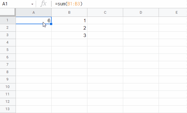
For instance:

In the above situation, you didn’t intend to divide by zero — it happened accidentally because of the values that were fed into your formula. You could easily fix this like so:

Now you’ve used the IF operator to tell Google Sheets to divide only if the number is more than 0.
You should always consider the fact that a value might not be what you expect it to be when you develop a sheet. Validate your data properly if you don’t want your sheet to break when it’s given unexpected data. There will be a time that someone enters in a “0” in a slot that shouldn’t hold an “0.”
#ERROR! – Your Entry Doesn’t Make Sense

An #ERROR! will occur if you’ve entered in something that does make sense in Google’s syntax, but it doesn’t actually amount to anything. In the above example, nested parentheses are frequently used to capture additional arguments and functions within a cell. But the nested parentheses don’t include anything.
Though this isn’t strictly wrong in terms of syntax, it also doesn’t mean anything. So, Google returns a rather generic #ERROR! as a request for you to fix not the syntax, but the logic. If you see an #ERROR! message, it’s likely that what you typed in doesn’t exactly do what you think it does.
How to Fix the Error
Note that as you type out a formula, Google Sheets will automatically start writing out that formula for you. You should be able to see which variables you need to pass to a given formula and how the formula will work (in brief).
Following along with the Google Sheets guide for the particular skill you’re learning will be an easy and simple way to learn how to use more functions. It’s often caused by missing parts in the function such as quotation marks, brackets, or commas.
#N/A – Your Item Was Not Found

The #N/A error generally occurs when something isn’t found that was expected. It’s most common when you’re using the LOOKUP, VLOOKUP, and HLOOKUP functions. You can also find it in more niche functions like IMPORTXML.
How to Fix the Error
In the above example, we’re using VLOOKUP to look up the number of Apples in a chart. But if we used “Kiwi” instead:

Now we get an #N/A error. An N/A error is a sign that we need to fix what we’re looking for. When it comes to a LOOKUP function, we could use “fuzzy” parameters (the best possible match) or we could simply validate the table first (make sure that something returns).
But #N/A doesn’t just occur when you’re using a LOOKUP function; that’s just when they’re the most likely. It’s so common that there’s a function called ISNA(), which can be used to validate your data and make sure that your information is used correctly. In other words, the best way to fix an #N/A error is to make sure the data in your table is valid.
#NAME? – You’re Incorrectly Applying a Label

#NAME? is a slightly more esoteric error condition. In Google, you can name a range; this makes it a “named range,” making it easier to reference.
How to Fix the Error
You must enclose the name within quotes (“Rainbow”). When you just use a word (Rainbow) it will pop up with #NAME?
If you want to name an importrange, you need to do it correctly. And make sure to validate the names that you do use. If you’ve never used a named range, you may want to look further into it — it can clean up and streamline your code.
#NULL! – You Are Using Microsoft Excel!
In fact, you shouldn’t see this error in your Google Sheet. #NULL! is a commonplace error in Microsoft Excel, when a value is returned that is empty though it is expected not to be. Google tends to be more forgiving than this, usually just treating a null value as a blank space or a zero, depending on needs. You can even set things to “null” without getting a #NULL! error.
For the most part, it’s not a terrible idea to assume that if something works one way in Microsoft Excel, it’ll work the same way in Google Sheets. But that isn’t always true. #NULL! is an excellent example.
#NUM! – Your Number is Too Large to Display

In this situation, a given calculated field is just too large to be displayed. The number that we’re trying to calculate is above the feasible limits of any system, so Google Sheets isn’t going to waste time trying to calculate it (and, ultimately, locking up your system).
Instead, Google Sheets will warn you about numbers that are outside of the range that can be depicted. If this happens to you during intense calculations, then you know that either something has gone wrong, or you need to wildly reduce the amount of precision that you’re dealing with.
How to Fix the Error
There may be times when you need a high level of precision or Very Large Numbers, but it’s unlikely that most people will ever stretch the capacity of Google Sheets’ cells. If you’re seeing the #NUM! error, it’s much more likely that you’ve accidentally typed something you didn’t mean to. Check your inputs.
To change the accuracy requirements, you can use the move decimal place shortcuts in the toolbar.
#REF! – Your Reference No Longer Exists

The #REF! Google Sheets error refers to a reference that doesn’t or no longer exists. In the above example, we’re referring to a sheet (Sheet2) that doesn’t exist, so we get a #REF! error.
But people don’t commonly refer to something that doesn’t exist altogether. Usually, this happens because a sheet gets deleted.
How to Fix the Error
Luckily, in Google Sheets you can always review previous iterations of a file. You can even launch it as a copy or replace the current file altogether. If you accidentally delete a reference, you can pull up an older sheet and see where that reference came from. You may also be able to press Ctrl + Z if deleting the reference in the same sheet was your last action.
#REF! will often show up if the cell your result is in is also in the specified range so you should remove it if that’s the case. For example, if your total is in cell B6 and your formula is =SUM(B1:B6) change it to =SUM(B1:B5).
#VALUE! – Your Item is Not the Expected Type

The #VALUE error in Google Sheets occurs when something isn’t the expected type. This error is simple to fix. In the above, we are trying to add together two strings. We can’t’ do that! If we replaced them with numbers, the formula would work fine.
Of course, it doesn’t always look that simple. You can get a #VALUE error with more complicated formulas, which requires that you look at the assigned values to ensure that the right value is being passed.
How to Fix the Error
Whenever you get a #VALUE! error, you should review the formula itself. You may be misusing the formula, which is what’s leading to the vague error.
“There was a problem” – You’ve Written Your Formula Incorrectly

This is the most common formula parse error in Google Sheets. It can also be one of the more frustrating errors to get. If you type something wrong (frequently, it’s just a typo), you’ll get a pop-up with “There was a problem.” This pop-up can be a little annoying because it’ll interrupt whatever you were doing. You’ll have to close the box and fix the syntax.
In the above screenshot, we just mistyped. We wanted to say “sum()”, but instead we ended up typing “sum()/”.
The “There was a problem” pop-up is distinct from #ERROR!. The #ERROR! appellation means that while the syntax appears to be correct, it doesn’t make sense to the compiler. You have technically typed something that is accurate, but it has no meaning.
Comparatively, a formula parse error means that your formula syntax does not make any sense. It will never run, even if the right values are fed into it. A formula parse error is fairly serious, but it’s also fairly trivial; it should be easy to tell what’s wrong.
Other Strategies for Dealing With a Formula Parse Error in Google Sheets
Using Google’s Built-In Error Documentation
At this point, you might have noticed that Google has a type of built-in error documentation. Every formula that Google Sheets supports is tied into a database within Google Sheets itself. As you start to type in formulas, you will see pop-ups guiding you through their completion.
Let’s revisit an error:

In the #ERROR! above, you might be tempted to believe that you’ve calculated a number too large. But this number isn’t too large at all. If it was, you’d be getting a #NUM! error, not an #ERROR! error.

Just hold your mouse over a cell with a red triangle in the upper right corner and you’ll see exactly what type of error you’ve received. In the above, you can see that it’s a “Formula Parse Error.” From there, you’ll hopefully notice the extraneous “_” that is holding the formula back.

Whenever you get an error, the first thing you should check is the red triangle. If you just hover over any errors you get, you’ll get more information about how to fix them. When in doubt, you can go to Google Sheets tutorial pages to learn more.
Functions to Help Deal With Formula Parse Errors in Google Sheets
IFERROR
The IFERROR() function is easy to use when you want to “clean up” errors. Wrap a function up with IFERROR(), and you can have the program take a different tactic entirely when errors are discovered, depending on what the discovered error is.
The syntax of IFERROR() is very simple:
IFERROR(value,[value_if_error])
So, it essentially operates as any IF command. If the cell has an error, it will print out the “value_if_error.” Otherwise, it will leave the cell alone. There are other ways to manage a cell, but IFERROR() is one of the simplest, cleanest, and most readable.
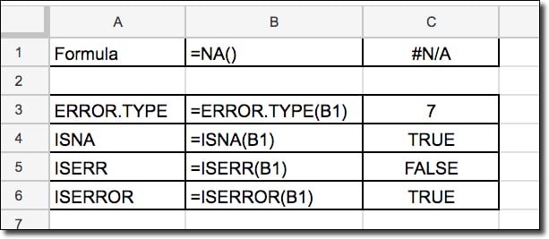
=ERROR.TYPE()
Gives the type of error through a numerical value:
- 1 = #NULL!
- 2 = #DIV/0!
- 3 = #VALUE!
- 4 = #REF!
- 5 = #NAME?
- 6 = #NUM!
- 7 = #N/A
- 8 = All other errors
=ISNA()
Provides a true value of there is an #N/A error in the specified range.
=ISERR()
Provides a true value if there is any other type of error in the specified range.
Reaching Out for Help
One of the major advantages of Google Sheets is that it has such a thriving community throughout the world. If you still can’t figure out how to fix your errors, you might not be alone. An online Google Sheets community (or even Google Sheets’ technical support) may be able to uncover problems that you have missed.
A primary benefit to Google Sheets is that you can add other people in as readers, commenters, and editors. If you’re struggling with your Google Sheet, consider sharing it with others who know the ropes. They’ll be able to get your issues fixed quickly through sheer experience.
Frequently Asked Questions
How Do I Fix a Formula Parse Error in Google Sheets?
First identify what the error code means. Mostly, there’s a missing reference or your formula is incorrect. Double check your formula against examples online.
What Is Parse Error in Google Spreadsheets? / What Does Formula Parse Error Mean?
Let’s take a quick look at formula to parse error meaning. A parse error in Google Sheets is a blanket term for a formula error. It accounts for the most possible problems that can occur when typing a formula. For example, #REF! means the reference does not exist in Google Sheets, so you should check the range in the formula is referencing an appropriate part of the spreadsheet.
How Do You Refresh Formulas in Google Sheets?
By default, formulas refresh when a change is made. But, you can also set them to refresh based on time by navigating to File > Spreadsheet settings > Recalculations and picking the appropriate option.
Why Is My Sum Formula Returning 0 Google Sheets?
The most likely explanation is that your values aren’t formatted as numbers. Make sure they are by using =ISNUMBER(cell range) in an empty cell, it will return FALSE if there are values that aren’t numbers in the range. Another possible reason is that you have an * in your formula and a null value cell. Anything multiplied by zero is zero.
Finding the Cause of Your Errors
Finding the cause of your formula parse error in Google Sheets begins with figuring out what the error code means. If you get an #ERROR! message, you know that there’s something wrong with your logic. If you get a #REF! message, you know that you probably just deleted a reference. If you get a #NUM! message, you know that you definitely tried to do something with numbers far too large.
Google Sheets, just like other complex software platforms, can require a bit of trial and error.
There will always be errors. Understanding these errors, being able to track them down, and being able to fix them will all make it easier for you to make useful and attractive spreadsheets.
Whether you’re just starting out with Google Sheets or are a seasoned pro, sooner or later one of your formulas will give you a formula parse error message rather than the result you want.
It can be frustrating, especially if it’s a longer formula where the formula parse error may not be obvious.
In this post, I’ll explain what a Google Sheets formula parse error is, how to identify what’s causing the problem, and how to fix it.
What is a formula parse error?
Before we get into the different types of errors, you might be wondering what does formula parse error mean?
Essentially, it means Google Sheets can’t interpret your formula. It can’t fulfill the formula request so it returns an error message.
There are a variety of ways this can happen — everything from typos to mathematical impossibilities — and we’ll explore them all in detail below.
Understanding the meaning behind the error messages, and learning how to fix them, is a crucial step to becoming a formula pro in Google Sheets.
Auditing and Debugging Formula Parse Errors in Google Sheets
Match the error message in your Google Sheet to the sections below, and find out what might be causing your error.
- An formula parse error message popup prevents me entering my formula
- I’m getting an #N/A error message
- I’m getting an #DIV/0! error message
- I’m getting an #VALUE! error message
- I’m getting an #REF! error message
- I’m getting an #NAME? error message
- I’m getting an #NUM! error message
- I’m getting an #ERROR! error message
- I’m getting an #NULL! error message
- Other strategies for dealing with errors
- Functions to help deal with formula errors in Google Sheets
- Help! My formula is STILL not working
Here’s a Google Sheet with all these examples in.
1. A formula parse error message popup prevents me entering my formula
You think you’ve finished your formula, so you hit enter and boom! You get slapped with a popup message box "Houston, we have a problem" or similar:
It’s reasonably rare that you’ll experience this, and it usually points to some fundamental problem with your formula.
For example, imagine that as you hit the Enter key, you also accidentally struck the “” key (which is right above the Enter key) and inadvertently added that to the end of your formula:
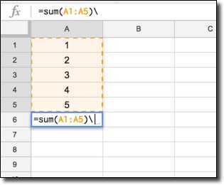
This will result in the popup error message. It’s easily corrected by removing the unwanted character.
How to correct this error?
Try to avoid these in the first place by checking your formula prior to hitting enter. Make sure you’re not missing a cell reference and you don’t have any unwanted characters lurking.
2. I’m getting an #N/A error message. How do I fix it?
The #N/A formula parse error signifies that a value is not available.
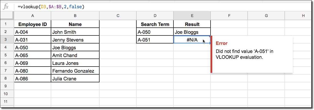
It happens most frequently when you’re using a lookup function (e.g. the VLOOKUP function) and the search term isn’t found. This is exactly what has happened in the exact match VLOOKUP in the image above. The search term A-051 is not in our data table so the formula returns #N/A.
This formula is not wrong or broken, so we don’t want to delete it. However, it would be cool if you could display a custom message, something like “Result not found”, instead of #N/A error message, especially if you have a lot of these errors showing. It gives the spreadsheet user much more information and reduces confusion.
Thankfully we can:
How to correct an #N/A error?
Well, there’s this super handy IFERROR function in Google Sheets:
=IFERROR(original formula, value to display if the original formula gives an error)
In this VLOOKUP example, the full formula would look like this:
=IFERROR(VLOOKUP(Search Term, Table, Column Index, FALSE),”Search term not found”)
as shown in this example:
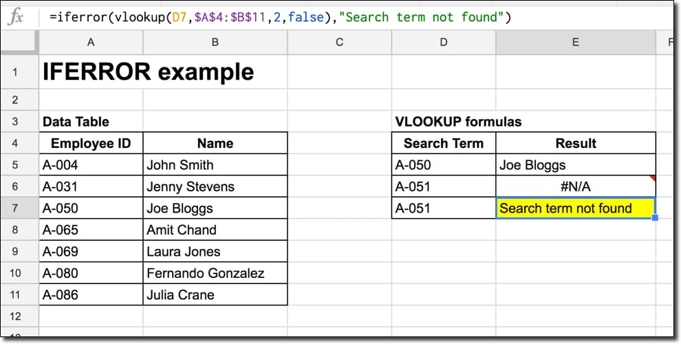
Instead of showing the #N/A formula parse error when a value is not found, the formula will output our custom message instead “Search term not found”.
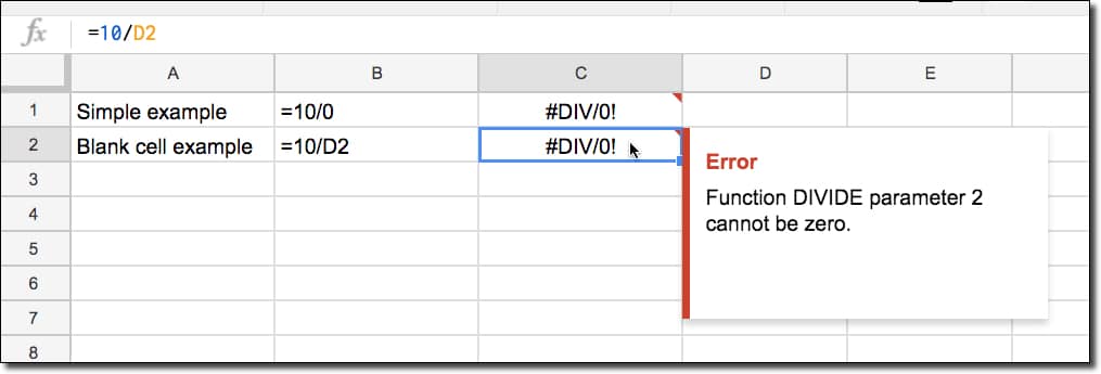
3. I’m getting an #DIV/0! error message
This formula parse error happens when a number is divided by zero, which can occur when you have a zero or a blank cell reference in the denominator.
In layman’s terms, what this means is that we’re trying to compute something like this:
= A / 0
which has no meaning because you can’t divide by 0.
Read more about division by 0 here, although it gets super technical super quickly.
Another example is using a formula like AVERAGE with a blank range.
= AVERAGE(A1:A10)
will cause a #DIV/0! error if the range A1:A10 contains no numerical values.
How to correct an #DIV/0! error?
Well, the first thing to do is determine why your denominator is evaluating to zero.
You can select the denominator and see what it is evaluating to by highlighting it in the formula bar, and seeing what the result is in the little popup box, as shown in this image:
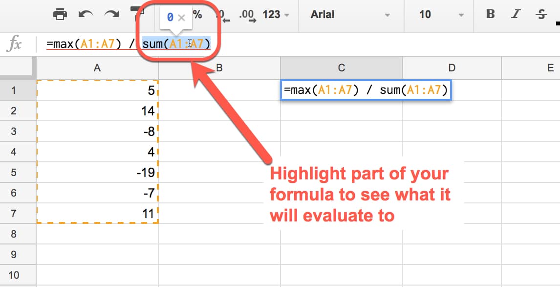
In this case, the formula in the denominator SUM(A1:A7) evaluates to 0, which causes the error. So check whether your denominator result is 0.
Next, check whether you have linked to blank cells or a blank range in your denominator. Then you can either fill in the blank cell or range, or select a different cell or range for your formula.
If your formula is correct and your cell/ranges are not unintentionally blank, then you’ll want to handle the #DIV/0! error. It looks unsightly and makes your spreadsheet look unfinished if you leave these errors floating around.
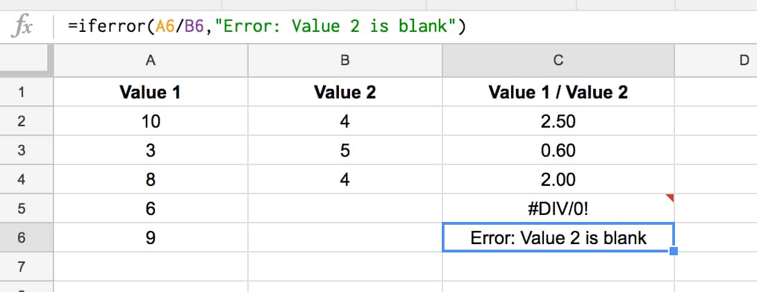
As with the #N/A error example, use the IFERROR formula to wrap your current formula and specify a result for when a #DIV/0! error occurs. You might want to output an error message, e.g. “Division by 0 error”, or maybe a specific value, e.g. 0:
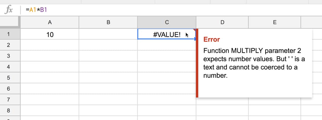
4. I’m getting an #VALUE! error message
This formula parse error typically occurs when your formula is expecting a certain data type as an input but receives the wrong type, for example trying to do math operations on a text value instead of a numerical value.
Spaces in your cells can also cause this error message.
In this example, cell B1 contains a space, which is a string value and causes the #VALUE! error because Google Sheets can’t perform a math operation on it, as seen in this error message:
In general, Google Sheets do a pretty good job of coercing text into numbers when needed. If you enter a value into a cell with some spaces, format it as text and then try to do math on it, Google Sheets will actually force the text into a number and still perform the calculation.
Another cause of #VALUE! errors is mixing US and Rest of World date formats.
US dates have the form MM/DD/YYYY whilst the Rest of the World goes for DD/MM/YYYY. If you have a mix of the two and try to subtract them to get the number of days between them for example, you’ll get the #VALUE! error.
(In fact, it’s the same text/number issue happening underneath the surface. Dates are stored as numbers, but if you’re date is in the wrong format for the country setting for your spreadsheet, it’ll be stored as a text string and Google won’t know it’s meant to be a date.)
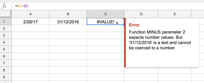
Here the correct answer should have been 59, the number of days between the 28 Feb 2017 and the 31st Dec 2016.
How to correct an #VALUE! error?
The error message should give you some information on which part of your formula is causing the problem.
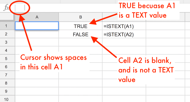
Search for any possible text/number mismatches, or cells containing errant spaces. If you click into a cell and the flashing cursor has a gap between itself and the element it’s next to, then you’ll have a space there.
Cells can look empty but still contain spaces:
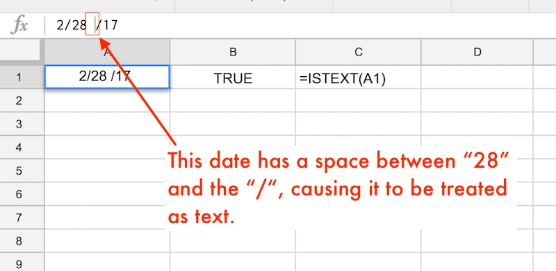
Dates with spaces in the middle won’t work either:
5. I’m getting a #REF! error message
The #REF! formula parse error occurs when you have an invalid reference.
Missing reference: For example when you reference a cell in your formula that has since been deleted (not the value inside the cell, but the whole cell has been deleted, typically when you’ve deleted a row or column in your worksheet).
In this example, the original formula was
= A1 * B1
but when I deleted column A, the formula went haywire because of the missing reference:
Another way that a formula can refer to missing references is when you copy a formula with a relative range at the edge of your sheet. When you copy and paste, it’s possible the relative range moves as if it were outside the bounds of the sheet, which is not allowed and will cause a #REF! error.
In this example, the sum function adds the cells in the 3 rows above. When I try to copy-paste the sum function into a new cell with fewer than 3 rows above, it’ll give me the #REF! error:
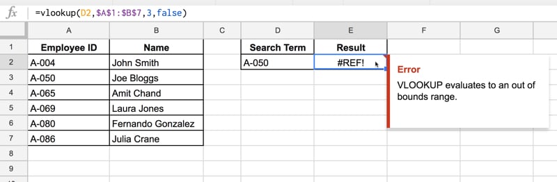
Lookup out of bounds: You’ve probably seen the #REF! error if you use lookup formulas frequently, when you’ve tried to return a value outside of ranges you’ve specified. In this VLOOKUP example, I’m trying to return an answer from the 3rd column of a search table that only has 2 columns:
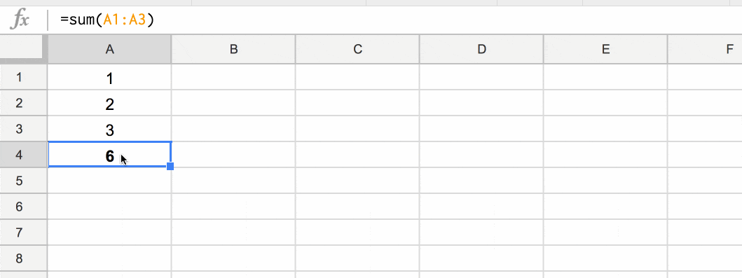
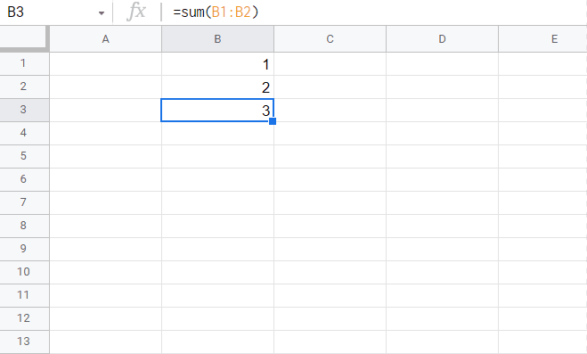
Circular dependency: You’ll also get a #REF! error when a circular dependency is detected (when the formula refers to itself).
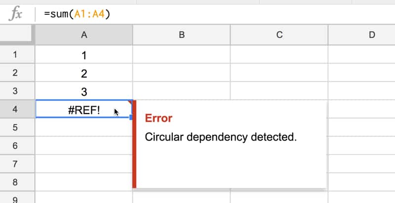
In this example, I have numbers in the range A1 to A3, but the SUM formula in cell A4 tries to sum from A1 to A4, which includes itself. Hence, we have a circular argument where cell A4 is trying to be both an input and output cell, which is not allowed.
How to correct a #REF! error?
First of all, read the error message to determine what kind of #REF! error you’re dealing with. This should give you a big hint on how to correct the error.
For deleted references, look for the #REF! error is inside your formula, and replace the #REF! with the correct reference to a cell or range.
For out-of-bound lookup errors, look through your formula carefully and check your range sizes against any row or column indexes you’re using.
For circular dependencies, find the reference that’s causing the problem (i.e. where you refer to the current cell inside your formula too) and modify it.
6. I’m getting a #NAME? error message
The #NAME? formula parse error signifies a problem with your formula syntax.
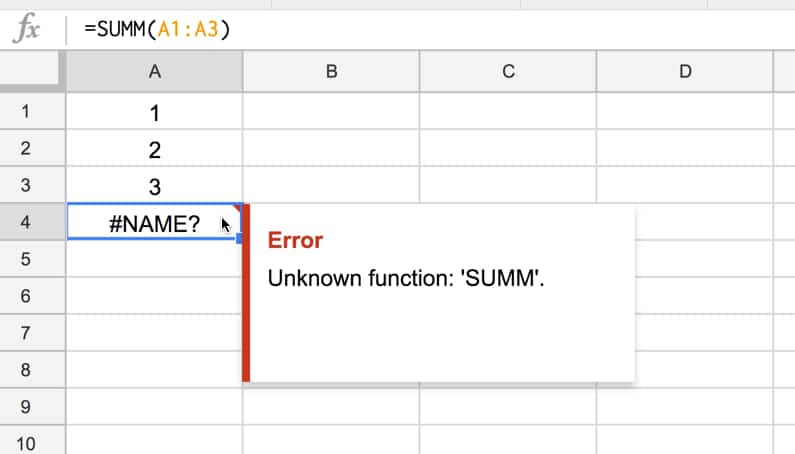
The most common reason for this error is a misspelling in one of your function names.
In this example, I misspelt the SUM function as SUMM, which Google Sheets didn’t recognize, so returned an error:
Another reason for a #NAME? error is referencing a named range that doesn’t actually exist or is misspelled.
So
=SUM(profit)
will give you a #NAME? error if the named range profit does not exist
Missing quotation marks around a text value, as shown in this simple formula, will also cause a #NAME? error:
=CONCAT("First",Second)
(The word Second is missing quotation marks.)
How to correct an #NAME? error?
Check your function names are correct. Use the function helper wizard to reduce the chances of errors happening, especially for the functions with longer names. As you start typing your formula, you’ll see a menu of functions, which you can select with the up and down arrows and Tab.
Check you have defined all named ranges before using them in your formulas and that they all have the correct spellings.
Check any text values are entered with the required quotation marks.
Lastly, have you missed the colon in your range references? It’ll be obvious because it won’t be highlighted correctly.
This formula
=SUM(A1A10)
is missing the colon between A1 and A10 and will throw a #NAME? error.
It should of course read:
=SUM(A1:A10)
7. I’m getting an #NUM! error message
The #NUM! formula parse error is shown when your formula contains numeric values that aren’t valid.
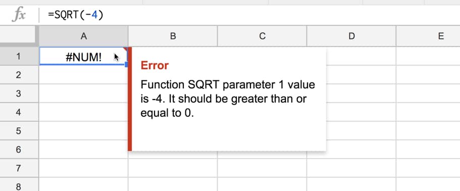
The classic example is trying to find the square root of a negative number, which isn’t allowed:
(For any math geeks out there, you’ll know that you can resolve square roots of negative numbers with complex (imaginary) numbers.)
Some other functions that can result in #NUM! error messages are the SMALL function and LARGE function. If you try to find the smallest n-th value in your dataset, where n is outside the count of values in your dataset, you’ll get a #NUM! error.
For example, you ask Google Sheets to find the 10th smallest number in a dataset that only has 5 values in it:
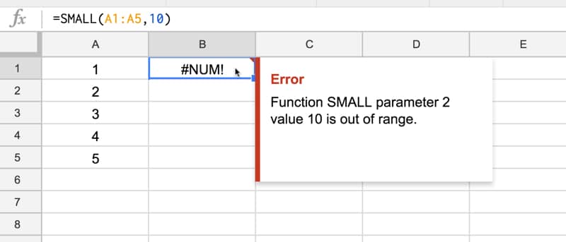
(Why this doesn’t return a #REF! error like the VLOOKUP out of bounds example, I don’t know.)
How to correct a #NUM! error?
You need to check the numeric arguments in your formula. The error message should give you some hints about which part of the formula is causing the issue.
8. I’m getting an #ERROR! formula parse error message
This formula parse error message is unique to Google Sheets and doesn’t have a direct equivalent in Excel. It means that Google Sheets can’t understand the formula you’ve entered, because it can’t parse the formula to execute it.
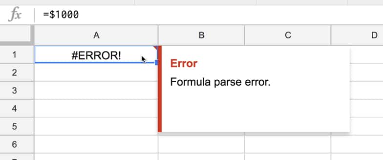
For example, if you manually type in a $ symbol to refer to an amount, but Google Sheets thinks you’re referring to an absolute reference:
or you’ve missed a “&” when concatenating text and numerical values:
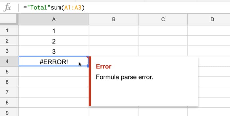
In this case the formula should be:
="Total "&sum(A1:A3)
Another case, caused when we messed up the closing brackets of a formula:
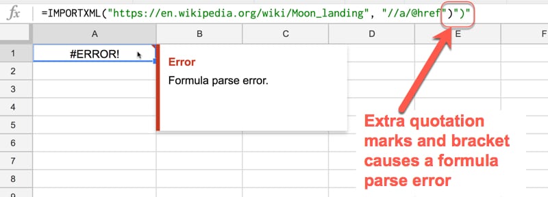
How to correct an #ERROR! error?
Carefully check your formula for accuracy.
You want to ensure you’ve got the correct number of brackets and correct join syntax between text and numerical values (e.g. using “&”).
When you want to show values with currency symbols or as percentages, don’t manually type in the “$” or the “%”. Instead, enter a plain number and then use the formatting options to change it to the style you want.
9. I’m getting an #NULL! error message
I haven’t been able to recreate a #NULL! formula parse error in the wild but theoretically, it exists!
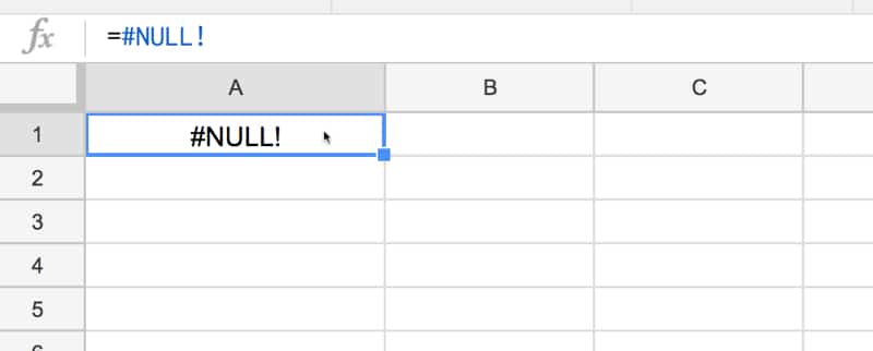
(If you have one showing in your sheet, let me know! I’d love to update this article with an example here.)
10. Other strategies for dealing with a formula parse error
Look for red highlighting in your formula as this will help identify the source of your error e.g. in the case of too many brackets, the extra, superfluous ones will be highlighted in red.
Peeling back the onion: the onion framework is a technique to debug errors for long, complex formulas. Unwrap the outer functions in your formula one-by-one, until you get it working again. Then you can start to add them back one-by-one again, and see exactly which step is causing the issue and fix that.
Different syntax in different countries: Some European countries will use semi-colons “;” in place of commas “,” so this could be a cause of your error. Compare these two formula, which have identical inputs and outputs, but the syntax is different for users in different countries (locales).
=ArrayFormula(VLOOKUP(A1;Sheet2!A:I;{2345678};FALSE))
is the same formula as this:
=ArrayFormula(VLOOKUP(A1,Sheet2!A:I,{2,3,4,5,6,7,8},FALSE))
(This is an example of a VLOOKUP returning multiple values (an array) instead of just a single value.)
Pro tip:
Use apostrophe at the start of a formula to turn it into a text string, which won’t execute. This is sometimes useful for seeing your whole formula for debugging, keeping a copy of your formula so you can copy and paste bits of it elsewhere for testing.
11. Functions to help deal with formula parse errors in Google Sheets
A few other functions related to formula parse errors are worth knowing about.
In fact, there is even a function to generate #N/A errors. It’s of limited use, but can be helpful for doing data validation in more complex formulas.
=NA()
will output an #N/A error. (Google Docs Help on NA)
=ERROR.TYPE(value)
will return a number corresponding to the error type:
- 1 for #NULL!
- 2 for #DIV/0!
- 3 for #VALUE!
- 4 for #REF!
- 5 for #NAME?
- 6 for #NUM!
- 7 for #N/A
- 8 for all other errors
(Google Docs Help on ERROR.TYPE)
=ISNA(value)
checks whether a value is the error #N/A, and will give the output TRUE for a #N/A error and FALSE otherwise. (Google Docs Help on ISNA)
=ISERR(value)
checks whether a value is any error other than the #N/A error. (Google Docs Help on ISERR)
=ISERROR(value)
checks whether a value is an error, and will give the output TRUE for any error. (Google Docs Help on ISERROR)
These functions can be summarized in the following table:
13. Help! My formula is STILL not working
Take a deep breath, don’t panic! There’s an army of Google Sheets super users out there who would love to help you fix your issue, free of charge, in the active help forums.
Try posting your problem into the forum and someone will likely help you out.
To make it easier for people to help you, please share your Google Sheet in view-only mode(how to share your Google Sheet) and include the error message and what you were expecting the correct answer to be.
You’re working in a spreadsheet and you want to use a function.

![→ Access Now: Google Sheets Templates [Free Kit]](https://no-cache.hubspot.com/cta/default/53/e7cd3f82-cab9-4017-b019-ee3fc550e0b5.png)
You write the formula, excited to get the results, then you see «Formula parse error» leaving you feeling confused and a little defeated.
Let’s cover what that actually means and what probably lead to that error message.
What is a formula parse error?
A formula parse error happens when you enter a formula into a cell, and the spreadsheet software cannot understand what you want it to do.
It’s like trying to speak a different language without taking the time to learn it first.
The software can kind of make out what you’re saying, but not well enough to give you an accurate result.
There are two likely causes for this error: There’s a typo in your formula, or the order of operations is unclear.
We’ll go over some examples of each so that you can identify and fix them in your own formulas.
Usually, a formula parse error happens because of:
Incorrect syntax – E.g.: Typing =+ instead of =, forgetting to put quotation marks around text values, putting two operators next to each other without anything in between them
Incomplete syntax – E.g. Leaving out a parentheses.
Another reason why you may be getting these errors is that you’re trying to use text values where numbers are expected.
Let’s dive into the specific types of errors you may encounter:
#N/A Error
One of the most common errors is the #N/A error. It occurs when a formula can’t find what it’s looking for.
For example, if you’re using the VLOOKUP function to find a value in a table, and the value you’re looking for isn’t in the table, you’ll get the #N/A error.
#DIV/0 Error
This happens when you try to divide a number by zero.
For example, if you have a formula =A17/B17 and the value in B17 is 0, you’ll get the #DIV/0! error.
#REF! Error
When a formula contains an invalid cell reference, you will get this error message.
For example, if you have a formula that references cells A17:A22 and you delete row 21, the formula will return the #REF! error because it no longer has a valid reference.
#VALUE Error
The #VALUE! error occurs when a formula contains an invalid value.
For example, if you have a formula that multiplies two cells and one of the cells contains text instead of a number, you’ll get this error.
#NAME Error
This error occurs when a formula contains an invalid name.
For example, if you have a named range called » Prices» and you accidentally type «price» in your formula, you’ll get the #NAME? error.
#NUM Error
The #NUM! error occurs when a formula contains an invalid number.
Say you have a formula that divides two cells and the result is too large to be displayed, you’ll get this error.
Now that we know what can cause a formula parse error, let’s look at how we can fix them.
How to Fix Formula Parse Errors
The best way to avoid getting formula parse errors is to carefully check your syntax as you type it out. If you’re not sure what order the operations should go in, refer back to the order of operations suggested by the software you’re using.
If you’re getting formula parse errors, here are some steps you can take to fix them:
- Check your formula inputs and make sure they’re correct.
- Use the IFERROR function and display a different result if an error occurs. E.g. «Not found.»
- Check your spelling and make sure all the parentheses are in the right places.
- Make sure you’re using the correct operators.
- Use cell references instead of hard coding values into your formulas.
- If you’re using text values, make sure they’re enclosed in quotation marks.
By following these steps, you can avoid formula parse errors and get accurate results from your formulas.

Formulas in Google Sheets were meant to make things easier for us.
However, every Formula user, regardless of whether it’s a beginner or expert, has invariably come across a formula parse error in Google Sheets at least once in their life (and if you haven’t. you soon will).
These errors can often be quite frustrating, especially if you don’t understand what they mean.
In this article, we will talk about each common formula parse error in Google Sheets, what they mean, and how to trace the cause and correct the problem.
What is a Formula Parse Error?
A formula parse error occurs when Google Sheets is unable to understand your formula. There may be a number of reasons for this, for instance:
- There might be a typo in the formula.
- There might be more or fewer parameters than the number expected for a specific function.
- One or more parameters entered might be of a different type from what is expected.
- Cell references in your formula might be out of bounds.
- You might be trying to do a calculation that is mathematically impossible.
There may be a number of other reasons, and all these reasons make it difficult for Google Sheets to fulfill what is requested by your formula. As such, it returns an error message.
We are going to take a look at some common error messages and explore what they mean in the following section.
Finding the cause of the problem is of utmost importance, in order to solve it. Thankfully, Google Sheets tries to help you out by suggesting what might be wrong with the formula, so you can break it down and detect the root of the problem.
Different Types of Formula Parse Errors in Google Sheets
Let us first take a look at what kinds of different error messages you are likely to see:
#N/A Error
This error usually occurs when a particular value that the formula needs is not present. The ‘N/A’ in the error message simply means ‘not available’. In other words, the value is not available for the formula to work on.
This problem is often encountered when you use lookup formulas like VLOOKUP in Google Sheets.
For example, if you’re looking for a value and that value does not exist in the given range, you will most likely see a #N/A error.
In the image below, the VLOOKUP function needs to find the value ‘Tom’ from the range A:B. But since the value ‘Tom’ does not exist in the range, the function simply returns a #N/A function to indicate that the value ‘has not been found’.

Related: Google Sheets VLOOKUP from Another Sheet
How to Fix the #N/A Error
The #N/A error does not always signify a problem with your formula itself, but a certain circumstance (the absence of a value) that results in an error.
To rectify this error, you can combine the formula with an IF statement that displays a custom message if the #N/A error is encountered. A very useful function to handle these kinds of issues is the IFERROR function.
For example, we rectified our problem below by using an IFERROR statement to display a “Search Value not found” message instead of an #N/A error:

#DIV/0 Error
This error occurs when a number in the formula is being divided by zero. This makes no sense mathematically, so the function returns a #DIV/0 error. For example, if you are trying to divide a value by a function or operation that results in a 0 value, you will get a #DIV/0 error.
In the image below, we are trying to divide the number 7 by the difference between values in A1 and A2, which results in 0. Since it is not possible to divide 7 by 0, the formula returns a #DIV/0 error.

This error also happens when you are trying to apply the AVERAGE function on a range of blank cells. This happens as the AVERAGE function needs to divide the SUM of the values with the number of the values, and if the range is blank, it’s equivalent to dividing by 0.

How to Fix the #DIV/0 Error
To resolve this error, you can try to first find out why your denominator is evaluating to a ‘0’ value. Select parts of the denominator in the formula bar to see what each part evaluates.
You can see the result of the calculation is a little popup right on top of the formula bar. Once you find the cause, you can make changes to your formula accordingly.

If that does not work, you can check if any part of the formula’s denominator links to a blank cell or range. If so, then you can either fill required values into the cell or select the required range for the formula.
To avoid problems like this altogether, you can again use the IFERROR statement to display a particular message whenever an error is encountered:

#REF! Google Sheets Error
This error occurs when you have an invalid reference in your formula. There may be different types of invalid references:
Missing Reference:
This kind of #REF! error occurs when you might be referencing a cell in your formula that is missing. In the image below, we have two values (45 and 50) in cells A1 and A2. We used the formula: =A1+A2 to find the sum of these two numbers in cell A3.

Till now it is fine. But what happens if we delete row 2? Then the value in cell A2 goes missing. This causes the formula in cell A3 to return a #REF! Error.

Circular Dependency:
This kind of #REF! error occurs when your formula might be referencing itself. In the image below, we used the formula =SUM(A1:A3) in cell A3. This means the formula, in addition to referring to values in A1 and A2, also refers to itself.

So the function will keep going round in circles trying to be both an input and an output cell, which would result in an infinite loop and a system crash. So to avoid this, the formula detects the circular reference and returns a #REF! error.
Lookup that is Out of Bounds:
This kind of #REF! error occurs when using VLOOKUP, and trying to reference a cell that is outside the bounds of the VLOOKUP range parameter.
In the image below, the VLOOKUP formula is trying to look for the search parameter in the third column of the source table, even though the range parameter specified only consists of 2 columns.
Since you’re trying to return a value outside the range specified by the formula, it returns a #REF! error.

How to Fix the REF Error
Read the error message to find out what kind of #REF! error your formula has. If there are missing references, you can see the exact reference that is erroneous in the formula bar. The reference causing the problem will be replaced with an #REF!.
Once you’ve identified which cell is missing, you can replace the #REF! with the correct cell reference.

If there’s a circular dependency issue, then you need to identify the range of cells in the formula and change it to make sure it does not include the current cell too.
Finally, if there’s an out of bounds error, then either make sure the search term exists in the search table or make required changes to the search term itself. You can also avoid this type of error from happening by using the IFERROR function.
#VALUE! Google Sheets Error
This error occurs when one or more parameters in your formula are of a different type than what is expected. So if a function only accepts numbers as a parameter, but you have a text value in the cell being referenced, then you will end up with a #VALUE! error.
In the image below, a backslash character () got added to the end of the number in cell A2 by mistake. So when we use the formula =A1+A2 in cell A3, we are trying to add a number to a text value, which is invalid. Therefore, the formula returns a #VALUE! Error.

Similarly, in the next image shown below, the cell A2 has a space in it, which makes it get treated as text. If the cell had been blank, then the ‘+’ operator would have assumed the value as a ‘0’.
Again, since we are trying to add a numeric value to a text value (‘ ‘), the formula returns a #VALUE! error.

How to Fix the #VALUE! Error
Once again, the error message should give you a clue about the source of the error.
To resolve the #VALUE! error, you can try one of the following:
#NAME? Error
This error commonly occurs when there is a problem with the syntax of your formula. It could be due to a spelling mistake, an incorrect named range, or the presence or absence of quotation marks.
For example, if you forget to add quotation marks around a string value, then the formula considers it as a named range, and if a named range by that name doesn’t exist then it returns a #NAME? Error.
In the image below, we did not put quotation marks around the first parameter of the CONCAT function, causing it to consider the first parameter “Peter” as a named range. Since it cannot find a named range by that name in the sheet, it returns a #NAME? error.

Related: Google Sheets CONCATENATE
Similarly, in the next image below, we misspelled the function name AVERAGE, causing the formula to return a #NAME? error.

Again, in the next image below, as you can see, we missed adding a comma in between the cell references A1 and A2. This is a syntax error, due to which the AVERAGE function returns a #NAME? error.

How to Fix the #NAME? Error
Since this kind of error usually occurs due to a syntax issue, the best approach is to first check if there are any spelling mistakes in the function name or named range names.
You can also check to see if all string values are enclosed in quotations and that there are both opening and closing quotations for every string value.
If using cell reference ranges, check to see if you have them separated by a colon symbol. (‘:’).
#NUM! Error
This error occurs when your formula has invalid numeric values. For example, if you try to find the square root of a negative number or if a calculation results in a very large number that is outside the scope of Google Sheets.
In the image below, we are passing a negative value to the SQRT function, which is not acceptable, so the function returns a #NUM! error.

Similarly, in the next image shown below, we are trying to find the result of 150 raised to the power of 200, which is a very large number (more than 1.79769e+308, which is the limit). The formula thus returns a #NUM! error.

How to Fix the #NUM Error
This error invariably means there’s an error with one or more of your numeric arguments.
Usually, the error message gives a good clue about the issue causing the error. For example, if the error message says “Function SQRT parameter 1 value is negative.
It should be positive or zero.” it’s quite clear that your first parameter in the SQRT function evaluates to a negative number.
So to resolve it, you can re-evaluate your calculation to make sure it doesn’t result in a negative number. To see what the result of an operation is, you can select the operation by highlighting it in the formula bar. You should be able to see the result of the calculation is a little popup right on top of the formula bar.

Keep in mind though, that if an operation evaluates to a very large number, you would not be able to see its result in the popup. This, in itself, can give you a sign of the source of the #NUM! error.
#ERROR! Message
This type of error is unique to Google Sheets. It usually occurs when Google Sheets cannot make sense of your formula, so it cannot tell you exactly what is wrong with it. There may be a number of reasons you see this error.
It may be because you forgot to add an important operator between cell references, values, or parameters. For example, forgetting to add a comma between cell references of non-contiguous cells in your sheet.

It could also be because your number of opening brackets doesn’t match the number of closing brackets. In the image below, we used a $symbol to refer to a price amount, but Google sheets mistake it for an absolute reference and the formula, then, does not make sense.

Sometimes this error also occurs if you don’t want to enter a formula, but want to start your text with an equal to sign (‘=’). However, as soon as Google Sheets sees the equal to sign, it assumes that you are trying to use a formula. But the text following the equal to sign does not make sense, so you get a #ERROR message.
How to Fix the #Error
Resolving this error can sometimes be tough, especially if you have a particularly complex formula. This is because the error message does not give any clues about the error. However, there are a few steps that you can take to see if it helps resolve the problem:
- Check if the number of opening and closing brackets match and that they do not cause any logical errors.
- Check if there are colons and commas separating contiguous and non-contiguous cell/range references.
- If using currency or percentage symbols, make sure you remove them before applying them to the formula. If you need to use them, you can enter them as plain numbers and later format the result with an added percentage or currency symbol.
Formula Parse Error Message Popup
You see this error message in the form of a popup that does not let you enter your formula until you resolve the error. One comes across this error quite rarely.

It usually occurs when there’s some fundamental problem with your formula. In most cases, you will see it if you accidentally entered a character or symbol in your formula before pressing the return key.
In the image below, we accidentally entered a backslash character at the end of the formula before pressing the return key. This type of mistake is quite common since the backslash key is right above the return key on the keyboard.

A mistake like this will most likely result in a formula parse error message popup.
How to Fix the Formula Parse Error Message Popup
It’s best to avoid this error from happening in the first place. Always double-check your formula before hitting the return key.
Make sure there are no surplus characters hidden in your formula. Also, make sure there are no missing characters or cell references.
The #NULL Error in Google Sheets
There’s no fix for this error. But only because it doesn’t exist in Google Sheets. It’s only an Excel error.
Functions to Help Fix Formula Parse Errors
There are a few functions that you can use to help identify formula issues and resolve them. Let’s take a look at them and what they do.
=ISNA(value)
Checks whether the cell has an #N/A error
=ISERR(value)
Checks for every other type of error (not including #N/A)
=ERROR.TYPE(value)
Shows the type of error by returning a number value:
- 1 for #NULL!
- 2 for #DIV/0!
- 3 for #VALUE!
- 4 for #REF!
- 5 for #NAME?
- 6 for #NUM!
- 7 for #N/A
- 8 for all other errors
Google Sheets Formula Pass Error Extra Tips
Sharing with Other Countries
Some international sheets may use semicolons ; instead of commas , so try changing those out if you’ve copy-pasted a formula.
Highlighting
If you double-click the cell with the formula, sheets will usually underline the misfunctioning part of the formula in red. That makes it easier to pick apart your formula.
Formula Parse Error in Google Sheets FAQ
What Does Formula Parse Error Mean?
A formula parse error essentially means there is an error in the way you’ve entered a formula into Google Sheets.
How Do I Remove Formula Parse Error?
Troubleshooting will remove a formula parse error. There are several different types of errors that can occur. Click the cell to find the type you need to fix then follow our guide to fix that particular error.
How Do I Stop Formula Parse Error in Google Sheets?
The most common reason for a formula parse error is a mistyped formula. So, to minimize them make sure you’ve got the syntax and the figures right.
How Do I Get Rid of DIV 0 in Google Sheets?
The #DIV/0 error occurs when the denominator results in a zero. You can’t divide by zero, so check your formula to find where the cause for this error could be popping up.
How Do I Fix the Error Number in Google Sheets?
The #NUM error occurs when the result unexpectedly returns a negative value in a formula that only works with zero or positive numbers. You need to find the part of your equation that is causing the negative value result.
Fixing Your Formula Parse Error Google Sheets Issues
In this tutorial we discussed formula parse errors in Google Sheets in detail, explaining what they are, why you see them, and how to resolve them. We hope our guidelines help you come to terms with parse errors in your Google Sheets. If you’re still having trouble fixing a formula parse error, feel free to ask about it in the comments below.

Spreadsheet Expert
at
Productivity Spot
|
+ posts
Sumit is a Google Sheets and Microsoft Excel Expert. He provides spreadsheet training to corporates and has been awarded the prestigious Excel MVP award by Microsoft for his contributions in sharing his Excel knowledge and helping people.
Formula parse errors in Google Sheets are frustrating.
That’s why this page teaches you what each formula parse error is, why they happen and how to fix formula parse errors, and how to get rid of errors in Google Sheets by stopping them from being seen.
Find out how to fix your error by clicking on what you’re seeing in Google Sheets (an error in a cell or the popup message below):
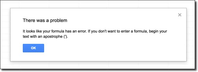
There was a problem
It looks like your formula has an error. If you don’t want to enter a formula, begin your text with an apostrophe (‘).
OK
Errors can be caused:
- Directly by the formula within that cell, or
- Indirectly when the formula in that cell references another cell that contains an error
#DIV/0!
You’ll see this error when you try to divide by zero… because you can’t divide by zero.
Here’s a simple example:
Function DIVIDE parameter 2 cannot be zero.
The #DIV/0! error happens whenever you use a function (or operator) that involves division when the number to divide by (denominator) evaluates to zero (including when you provide a blank cell).
Here are just a few examples of functions that can create this error:
- DIVIDE
- QUOTIENT
- MOD
- AVERAGE
- AVERAGEIF
How To Fix A #DIV/0! Error
You need to find the zero (or blank cell/s) causing the error.
This is easy in simple formulas but more difficult in complex ones.
Here’s a neat trick to help out.
When you’re typing your formula you can highlight complete functions (including those with nested functions) to see a little tooltip that contains the output:
This only works when the output is a single text, number, or BOOLEAN value.
If the highlighted function outputs an array of values it won’t be displayed.
When you find the guilty 0 (or blank cell), you can change it.
However, if the data is variable or you can’t control it (e.g. it comes from a Google Form) you can account for the potential of a zero denominator with a function like IFERROR.
=IFERROR(value, [value_if_error])
This function outputs the value if it isn’t an error.
If the value is an error, it instead outputs the entered [value_if_error] or nothing (if omitted).
From the first example:
=IFERROR(1/0, «Can’t divide by zero»)
Would output «Can’t divide by zero» instead of a #DIV/0! error.
This might not be an ideal solution in more complex formulas that could output more than one type of error.
For that, you might want to get more specific with your error handling using the ERROR.TYPE function which outputs 2 if its input results in a #DIV/0! error.


FREE RESOURCE
Google Sheets Cheat Sheet
12 exclusive tips to make user-friendly sheets from today:
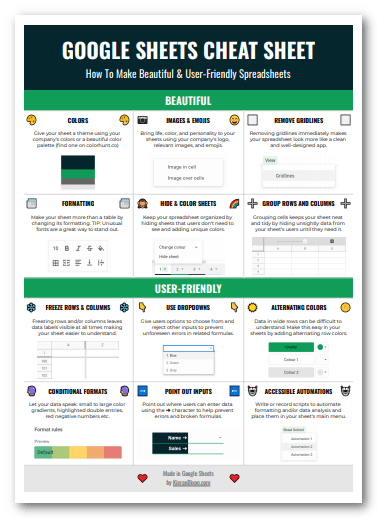
You’ll get updates from me with an easy-to-find «unsubscribe»
link.
#ERROR!
You’ll see this error when Google Sheets can’t understand (parse) your formula.
It’s trying to read it, but it just can’t for some reason.
Here’s something that can cause it:
Formula parse error.
Multiple arguments provided to the SUM function need to be separated by a comma. Without the comma, Google Sheets can’t understand what it’s supposed to do and throws the error.
#ERROR! doesn’t happen with specific operators or functions but instead can happen in any formula.
It just takes one syntax error to ruin the whole thing.
Can you find the error in this formula?
How To Fix An #ERROR! Error
Go back over your formula and check each function to make sure you’re not missing important syntax.
You’re looking for missing (or unnecessary additional) syntax in between values, functions, and arguments in your formula.
Keep an eye out for:
- Parentheses ()
- Braces {}
- Colons :
- Ampersands &
- Commas ,
- Dollar signs $
- Percentage symbols %
You should find (and be able to fix) the problem by reviewing these things.
For those playing along: the formula above was missing an ampersand to concatenate the data points:
#N/A
The output you want is Not Available.
That’s what #N/A means.
This error usually comes up when a function is looking something up and it isn’t there.
Functions like VLOOKUP and MATCH search columns for specific data and when they can’t find it, you get an #N/A error:
Did not find value ‘search_key’ in VLOOKUP evaluation.
Here’s an example:
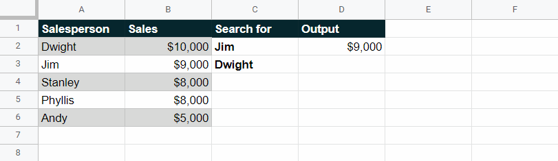
| A | B | C | D | E | |
| 1 | Salesperson | Sales | Search for | Formula | Output |
| 2 | Dwight | $10,000 | Stanley | =VLOOKUP(C2,$A$2:$B$6,2,0) | $8,000 |
| 3 | Jim | $9,000 | Pam | =VLOOKUP(C3,$A$2:$B$6,2,0) | #N/A |
| 4 | Stanley | $8,000 | |||
| 5 | Phyllis | $8,000 | |||
| 6 | Andy | $5,000 |
In the formula in D3 we’re searching for ‘Pam’ in column A.
VLOOKUP can’t find Pam and, as such, returns #N/A.
How To Fix An #N/A Error
An #N/A error can come from:
- A mistake in your formula
- The thing you’re looking not being there
Check your formula
With lookup formulas you have to provide a range to search and a search_key to find:
=VLOOKUP(search_key, range, index, [is_sorted])
As a general rule, this range should be an absolute reference ($A$2:$B$6 not A2:B6) so that if you fill or copy the formula elsewhere, the range to be searched doesn’t change:
You should also check that your search_key is what you expect it to be.
Be careful of trailing spaces that you can’t see (like «Pam «).
Use the TRIM function to remove leading and trailing spaces from your search_key (and your range if you want to be really careful) so that you don’t get an #N/A error from something you can’t even see.
Search_Key Not In Range
It could just be that the thing you’re looking for isn’t there.
If this is the case, you might want to use the IFERROR function
=IFERROR(value, [value_if_error])
This function outputs the value if it doesn’t result in an error.
If the value outputs an error, it instead outputs the entered [value_if_error] or nothing (if omitted).
From the example above:
- value = the VLOOKUP function
- [value_if_error] = a custom error message
| A | B | C | D | E | |
| 1 | Salesperson | Sales | Search for | Formula | Output |
| 2 | Dwight | $10,000 | Stanley | =IFERROR(VLOOKUP(C2,$A$2:$B$6,2,0),«Not found») | $8,000 |
| 3 | Jim | $9,000 | Pam | =IFERROR(VLOOKUP(C3,$A$2:$B$6,2,0),«Not found») | Not found |
| 4 | Stanley | $8,000 | |||
| 5 | Phyllis | $8,000 | |||
| 6 | Andy | $5,000 |
That’s much better than seeing an error.
This might not be an ideal solution in more complex formulas that could output more than one type of error.
For that, you might want to get more specific with your error handling using the ERROR.TYPE function which outputs 7 if its input results in a #N/A error.
#NAME?
This error appears when you’ve got the name wrong for a:
- Function
- Named range
Functions
In formulas, anything outside of a text string that precedes an opening parenthesis ( is assumed to be the name of a function.
If you spell the name of a function incorrectly, you’ll get an error:
Unknown function: ‘SOME’.
To avoid this mistake in the first place, take advantage of the function autocomplete helper that appears as you type:
Named ranges
Named ranges allow you to reference specific data using an easily understood and remembered piece of text.
If you name a column of sales figures ‘sales’, you can reference that data in formulas far more easily:
Misspelling a named range:
Results in a #NAME? error:
Unknown range name: ‘SAILS’.
This error can be caused by other syntax errors.
For example, if you accidentally leave out the double quotes around a text string:
Or miss out on colon in a range:
You will get a #NAME? Error that says «Unknown range name».
Always double check your formulas to make sure they are syntactically correct.
How To Fix A #NAME? Error
If the error message says:
- Unknown function: ‘NAME’
- You need to find the included ‘NAME’ function in your formula and change it to a known Google Sheets function.
- Unknown range: ‘NAME’
- You need to find the included ‘NAME’ range in your formula and:
- Change it to the correct name of an existing named range
- Create a named range with the included ‘NAME’
- Add double quotes around the ‘NAME’ to make it a text string
- Include a colon in the correct place to make it a valid range reference
- You need to find the included ‘NAME’ range in your formula and:
Handling errors using the IFERROR or ERROR.TYPE functions doesn’t really make sense because you want to know when something like this happens.
However, for your information ERROR.TYPE outputs 5 if its input results in a #NAME? error.
#NULL!
In Excel, specific circumstances produce the #NULL! error.
In Google Sheets those same circumstances do not produce a #NULL! error.
I can only assume that the #NULL! error was included in Google Sheets to:
- accommodate conversions from Excel to Google Sheets, and
- ensure compatibility with necessary functions
For example, both the IFERROR and ERROR.TYPE (outputs 1) functions handle #NULL! without issue.
I tried to write a formula to create this error but it seems the only way to produce a #NULL! error in Google Sheets is to type it in directly.
I even created a custom function exclusively to return a null value:
function RETURNNULL() {
  return null;
}
And it still didn’t throw the error!
#NUM!
The #NUM! error occurs when a number-based calculation won’t work.
Here are a few examples:
Impossible math
If you try to find the square root of a negative number:
A #NUM! error tells you this can’t be done:
Function SQRT parameter 1 value is negative. It should be positive or zero.
This is because the associated functions don’t handle imaginary numbers.
The same thing happens when using an operator instead:
POWER evaluates to an imaginary number.
Output is too big or too small
Google Sheets only recognises numbers between —1.79769E+308 and 1.79769E+308.
Anything outside of these bounds results in an error:
Numeric value is greater than 1.79769E+308 and cannot be displayed properly.
Numeric value is less than -1.79769E+308 and cannot be displayed properly.
Function-specific #NUM! errors
There are a lot of possible #NUM! errors in calculation-based functions.
Here’s three of them:
DATEDIF
The DATEDIF function calculates the time between two dates:
=DATEDIF(start_date, end_date, unit)
However, the start_date and end_date must be in chronological order.
If you provide a start_date that occurs after the end_date you will get a #NUM! error:
Function DATEDIF parameter 1 should be on or before Function DATEDIF parameter 2.
SMALL & LARGE
The SMALL and LARGE functions return the nth smallest or largest value from a dataset:
However, if the nominated n is not one of the viable options (from 1 to the size of the dataset) you receive this #NUM! error:
Function SMALL/LARGE parameter 2 value 7 is out of range.
The exact same thing happens when using the INDEX function and specifying a row or column that’s not available based on the provided reference:
=INDEX(reference, [row], [column])
Iterative Functions
Functions like IRR, RATE, and XIRR use iterative calculations to determine their output.
This means they calculate over and over again until they get the result they’re looking for.
You can provide arguments to these functions that would take a lot of iterations to solve. As such, Google Sheets imposes an internal limit on these iterations.
If your calculation is taking too many iterations, you’ll see this error:
IRR attempted to compute the internal rate of return for a series of cash flows, but it was not able to.
While testing the IRR function for this #NUM! error I found another:
In IRR evaluation, the value array must include positive and negative numbers.
The #NUM! error can pop up in unexpected places which is why it’s a good idea to have a general rule on how to resolve these issues.
How To Fix A #NUM! Error
The first thing to do is read the error message.
It will usually be explicit and help you get the heart of the problem quickly (as you can see from the above examples).
Once you know roughly what to look for, review your formula’s relevant numeric arguments.
Afterall, the #NUM! error is concerned with numbers.
Handling errors using the IFERROR or ERROR.TYPE functions (or similar) doesn’t really make sense because you want to know when something like this happens.
However, just FYI ERROR.TYPE outputs 6 if its input results in a #NUM! error.
#REF!
The #REF! error concerns invalid references in your formula.
Here are a few ways it can come about:
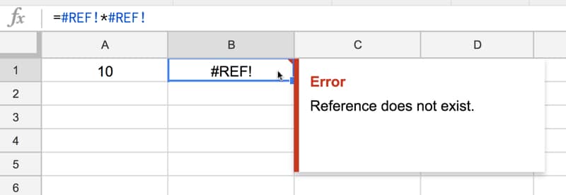
The Reference Doesn’t Exist
This can happen when you accidentally delete a cell that is referenced by a formula:
It also happens when you copy a formula with a relative reference to a part of the sheet that doesn’t have a valid cell in the relative position (usually near the boundary of the sheet):
Copying the formula =SUM(B1:B2) from B3 to A2 changes the B1:B2 relative reference to A0:A1 which doesn’t exist.
In both situations you’ll see this message:
Reference does not exist.
VLOOKUP #REF! Error
One of VLOOKUP’s required arguments is the column index from which to return a value:
=VLOOKUP(search_key, range, index, [is_sorted])
If you provide a number that is not within the bounds of the accompanying range you will receive a #REF! error:
VLOOKUP evaluates to an out of bounds range.
HLOOKUP throws the exact same error for its index:
=HLOOKUP(search_key, range, index, [is_sorted])
Circular Dependency
Referencing the cell that contains a formula within that formula causes a circular dependency.
For example, including =SUM(A1) in A1.
Without iterative calculation enabled the cell will present a #REF! Error:
Circular dependency detected. To resolve with iterative calculation, see File > Spreadsheet Settings.
This is because it’s impossible for a cell to use its own output as an input to generate that output.
How To Fix A #REF! Error
Handling #REF! errors using the IFERROR or ERROR.TYPE functions doesn’t make sense because you want to know when they happen.
If you do need to know: ERROR.TYPE outputs 4 if its input results in a #REF! error.
The error message attached to your #REF! error is the best way to figure out how to fix it:
Reference does not exist
Search your formula for the reference that is now #REF! and replace it with the correct reference.
If your #REF! error has just occurred you can undo (Ctrl+Z or ⌘Z) recent actions to try to figure out exactly what went wrong.
You can help to avoid creating these errors when copying and pasting formulas by relying on absolute references when they are appropriate.
Out of bounds range
Try to figure out why the index in your lookup function is evaluating to a number that doesn’t fit within the range.
Most often this is simply a typo.
Circular dependency detected
Double check where in your formula a cell or range reference includes the cell that contains your formula.
If this was intentional you can turn on iterative calculation to attempt to resolve the error. Go to ➜ ➜ :
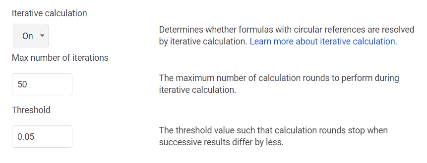
Having iterative calculations enabled may impact the performance of your sheet.
#VALUE!
The #VALUE! error pops up when a function expects a specific type of data (most often numbers) and instead gets something else (most often text):
Function ADD parameter 2 expects number values. But ‘two’ is a text and cannot be coerced to a number.
As the error message suggests, Google Sheets will do its very best to try to make (coerce) text into a number. That’s why this:
Works perfectly. The text » 2 « can be recognised as the number 2.
Some functions (including SUM) ignore data of the wrong type and won’t throw the #VALUE! error.
The #VALUE! error comes up a lot when dealing with dates and date-related functions.
In Google Sheets dates are just numbers.
When dates are typed in as text like «thu 16 dec 21« Google Sheets does an amazing job of converting it to a date (12/16/21).
Issues arise when spaces are included «12 /16/21« or there is confusion between formatting dates as mm/dd/yy and dd/mm/yy (you must use the one assigned based on the sheet’s locale [ ➜ ➜ ] with the other recognized as text).
How To Fix A #VALUE! Error
Use the error message as a hint before searching through your formula and referenced cells to find where a value you expect to be a number is actually text.
If you can’t find the source of a #VALUE! error try looking for blank cells using the ISBLANK, LEN or ISTEXT functions.
Sometimes cells you think are blank are actually full of spaces!
Handling #VALUE! errors using the IFERROR or ERROR.TYPE functions doesn’t make sense because you want to know when they happen.
If you do need to know: ERROR.TYPE outputs 3 if its input results in a #REF! error.
You type in a formula, hit Enter / Return and see this:
There was a problem
It looks like your formula has an error. If you don’t want to enter a formula, begin your text with an apostrophe (‘).
OK
Not to worry — this is usually an easy fix.
You’ll usually get this error because of a simple typo.
Here’s a common one — accidentally including too many parentheses:
They highlight it in red and everything but it’s still easy to miss.
Check the last few characters of your formula to make sure there’s no unnecessary extras.
Handling Formula Errors
There are a number of functions to help you handle errors in Google Sheets:
=IFERROR(value, [value_if_error])
IFERROR is the error-based function you’ll use the most.
It allows you to predict potential errors and prevent them from affecting other parts of your sheet by providing a backup value if the actual value is an error.
The ERROR.TYPE function is for serious error handling. It returns a number corresponding to the specific error encountered:
- #NULL!
- #DIV/0!
- #VALUE!
- #REF!
- #NAME?
- #NUM!
- #N/A
- All other errors
ERROR.TYPE could be paired with SWITCH or IFS to create a powerful error handling formula that responds differently to each error:
=IF(NOT(ISERROR(A1)),A1,SWITCH(ERROR.TYPE(A1),1,«Handle #NULL!»,2,«Handle #DIV/0!»,3,«Handle #VALUE!»,4,«Handle #REF!»,5,«Handle #NAME?»,6,«Handle #NUM!»,7,«Handle #N/A»,8,«Handle all other errors»,«»))
Creates an #N/A error.
It doesn’t seem particularly useful but can be used to indicate missing information more effectively than a blank cell and prevent further calculations that depend on it.
=IFNA(value, value_if_na)
Exactly the same as IFERROR but only provides the backup value_if_na if the error is #N/A.
Checks value and returns TRUE if it’s an error or FALSE if it’s not an error.
Checks value and returns TRUE if it’s an #N/A error or FALSE if it’s not an #N/A error.
Checks value and returns TRUE if it’s any error except #N/A or FALSE if it’s an #N/A error or any other value.
FREE RESOURCE
Google Sheets Cheat Sheet
12 exclusive tips to make user-friendly sheets from today:
You’ll get updates from me with an easy-to-find «unsubscribe»
link.

Kieran Dixon started using spreadsheets in 2010. He leveled-up his skills working for banks and running his own business. Now he makes Google Sheets and Apps Script more approachable for anyone looking to streamline their business and life.
You might like:
A formula parsing error message appears when the formula inputted expects a specific data type, but it received the incorrect kind. In other words, Google Sheets is unable to interpret your formula. It returns an error message since it is unable to complete the formula request.
It can be aggravating, especially if the formula is lengthy and the parsing problem isn’t apparent.
Do not worry! We would teach you how to identify the possible causes of the parsing problem and how to fix them!
Here are the five most common formula parse errors in Google Sheets that you may face:
- #N/A
- #DIV/0!
- #VALUE!
- #REF!
- #NAME?
Look familiar? Let’s see how to solve these errors! 🤗
Table of Contents
- Solve a #N/A Error in Google Sheets
- Solve a #DIV/0! Error in Google Sheets
- Solve a #VALUE! Error in Google Sheets
- Solve a #REF! Error in Google Sheets
- Solve a #NAME? Error in Google Sheets
Solve a #N/A Error in Google Sheets
When a #N/A error appears, it means that a value is not available. This error would be seen frequently when using the VLOOKUP function, as the search key cannot be found.
However, in this scenario, it does not mean that the formula we inputted is wrong. When the formula returns a #N/A error, it only means the specified search key is not within the range selected.
Let’s use an example to get better visualization.

As you can see from this example, Search Key B’s return value came back as an #N/A error. This is because the search key inputted “B2-05” could not be found in the range selected “A5:B9”.
Hence, this would cause the formula to return a #N/A error signifying the search key we inputted could not be found.
Solve a #DIV/0! Error in Google Sheets
#DIV/0! error appears when the formula divides a number with the value zero. This can happen when the denominator is zero. This does not make sense mathematically, so the formula returns a #DIV/0! error.

This error can also appear when the denominator is blank as well.

As you can see, since B1 does not have a value, the formula could not divide 40 by zero.
You would also often see this when using the AVERAGE function. The error would appear when the range selected for the formula is empty.

Simply make sure the denominators used or selected has a value, and this parse error would not appear again!
Solve a #VALUE! Error in Google Sheets
When one or more parameters in your formula are of a different type than expected, you’ll get this error. So, if a function only accepts numbers as an argument, but the cell being selected has a text value, you’ll get a #VALUE! error.
Spaces within your cells can also cause this error.

Even though A2 looks like an empty box, but we have inputted a space within the cell. This caused the formula to return a #VALUE! error.
Here is another example:

Here we can see that the formula inputted is multiplying a number value with a text value which is “five”. This formula does not make sense mathematically as well as the parameters in the formula are of different types.
To fix this error, make sure the cells selected contain the same parameter type. To perform a math operation, always remember to use numeric values only.
Another scenario in which this error might occur is when mixing the dates format in a formula.
US date format: MM/DD/YYY
Rest of the world: DD/MM/YYYY

As you can see, when subtracting the two dates, Google Sheets could only read 12/25/2021 as a date as it is a number value. Google Sheets reads 25/11/2021 as a text, hence the formula returns a #VALUE! error.
To fix this, simply make sure the dates entered into cells are in the same formats.
Solve a #REF! Error in Google Sheets
When you have an invalid reference, the #REF! error occurs. The most common situations are when the cell selected is missing or when the formula is referring to itself.
Missing Reference:
This often happens when the original cell selected has been deleted (when you delete a whole row or column).

After we delete column A, the formula goes haywire as they could not find the original A1 selected.

Another scenario is when we copy a formula with a selected range at the corner of your Google Sheets.
It’s possible that when you copy and paste, the relative range shifts outside the confines of the sheet, which isn’t allowed and will result in a #REF! error.


When we copy the formula SUM(A1:B1) to B2, it will result in a #REF! error. This is because the original formula has two columns selected, but when the formula is copied and pasted into B2, it is missing one more column.
Circular Dependency:
When the formula you entered is referencing itself, it is known as circular dependency. This happens when we selected a range that also consists of the formula itself.

As you can see, the formula contains a selection of cells that includes the formula itself.
Simply make sure that when you select the cells to be inputted, always exclude the formula to avoid such errors appearing.
Solve a #NAME? Error in Google Sheets
The #NAME? error appears when the syntax of the formula inputted has a problem. Most commonly, it is when the function name itself is misspelled.

The error would also appear when the named range does not exist.
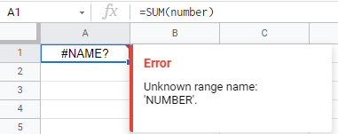
Another scenario is when a text value inputted is missing the quotation marks. This would also cause the #NAME? error to appear.

When done correctly, the error would not appear.

When the #NAME? error appears, making sure that the function name and range names are valid to avoid this error.
You may make a copy of the spreadsheet using the link attached below and try it for yourself:
There you go! After learning about these five commonly appear formula parse errors, would do not need to worry when they appear. Always make sure to understand what the error is trying to signify and fix the problems in the formula accordingly. 🎇

Get emails from us about Google Sheets.
Our goal this year is to create lots of rich, bite-sized tutorials for Google Sheets users like you. If you liked this one, you’ll love what we are working on! Readers receive ✨ early access ✨ to new content.
Encountering a parse error on Google Sheets is quite common for newbies as well as for experienced professionals. It is the way of the Sheets to tell you that there is something not right with your formula and Sheet cannot process the instructions given in the formula. These parse errors could be quite frustrating as you are expecting a calculated result but are “greeted” with the parse error, especially, if the error is occurring in a lengthy formula and the cause of the parsing error is not apparent.
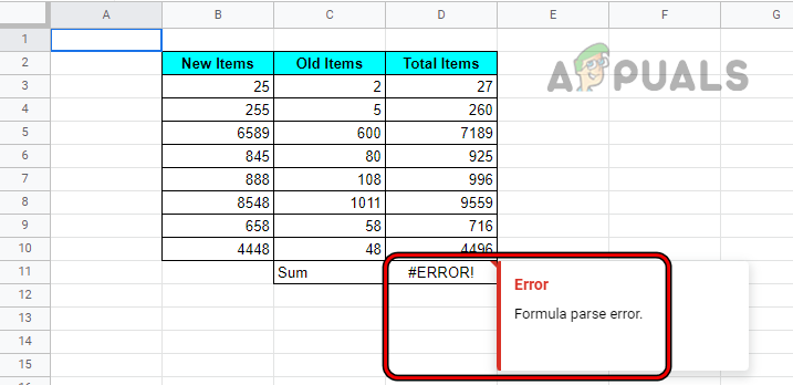
Once the Sheets show a parse error, it is simply telling you to correct your formula, arguments, data types, or parameters. A formula parse error is not a single error, there are many other errors under its hood like #N/A error, #error, etc. The parse error does not directly show in a wrong formula, it shows an error (like #error) but when you click on the error, then, in the side dropdown, it says formula parse error as shown in the image below where #Error! Is occurring in cell D11 but when clicked, it shows a formula parse error.
Google Sheets does not have a compiler (usually, linked to a parse error in the computing world). When a formula is entered in a Google Sheet, Sheets breaks down the syntax of the formula to analyze, categorize, and understand the syntax by using the parsing function. The parsing process consists of text dissection and the text is converted into tokens.
The Sheets parser function will then build a structure based on these tokens and other data received. If Sheets fail to perform the above on any of the formulae, then it will return a parse error. In simple words, parsing is dividing a large structure into smaller logical units for easier data storage and manipulation. Then Sheets re-compiles these as per the instructions and if any of these fail, that may lead to the Formula parse error.
Common Reasons for a Parse Error on a Google Sheet
The following are common reasons for which you may encounter a parse error:
- There is a typo in your formula like forgetting to put quote marks around a text string, putting two Sheets operators next to each other without anything to separate them. Also, an incomplete syntax (e.g., a missing parenthesis at the end of the formula) can cause a formula parse error.
- You have entered too few arguments or too many arguments as per the function’s requirements.
- The data types of the parameters of the formula are different from what Sheets is expecting like performing an addition operation on a text string will result in a parse error.
- The formula is trying to do an impossible mathematical operation (like dividing a value by zero or an empty cell).
- The formula is referring to an invalid cell range or the file you are referring to does not exist or is not accessible.
Types of Formula Parse Errors on a Google Sheet
The following are the most common types of parse errors on Google Sheets.
- There was a Problem Pop Up: When you encounter this type of error on Google Sheets, it means that the formula you entered is incorrect like adding a / at the end of the formula where it is not required.
- #N/A Error: This error means that your item was not found. Simply, the formula is searching for an item that does not present in the data.
- #Div/0 Error: This error means that you are trying to divide a value by zero. It implies that the formula calculations involve a step where the value is divided by zero, which is mathematically impossible.
- #Ref Error: This error means that your reference no longer exists. We can apprehend that the cells, files, links, images, etc. that the formula is referring to do not exist or is not accessible.
- #Value Error: This error means that your item is not of the expected type i.e., if you are adding two cells but one of the cells contains a text string, then the addition formula will return a #value error.
- #Name Error: This error means that you are incorrectly applying a label. For example, if you are using a named range in your formula, either you forget to add double quotes around it or the range name is not valid, then that would result in a #name error on a Google Sheet.
- #Num Error: If the result of a formula calculation is a very large number that cannot be displayed or is not valid, then that would result in a #num error on a Google Sheet like a square root of a negative number.
- #Null Error: This error means that the returned value is empty though it should not be. This error pertains to Microsoft Excel and is not a native error on Google Sheets. This error can only be cleared in Excel, not Google Sheets.
- #Error Error: If anything in your formula does not make sense to Google Sheets but Sheets are failing to point out the culprit (like a number issue by showing a #num error), then that could result in a #error. This type of error can sometimes become tough to troubleshoot as it is more generic, as all other ones are a bit specific. In other words, if an error does not fall in any other error types, Sheets will show #error for that error.
Fixes for a Parse Error on a Google Sheet
As we have covered the basics of the parse error, let us focus on troubleshooting it. But keep in mind that there is not a single size that fits all the scenarios and the troubleshooting process differs on a case-to-case basis. Let us discuss each error type with examples.
1. #N/A Error
This error is derived from the phrase “Not Available”. It mainly occurs in Lookup, HLookup, ImportXML, or similar functions which find a particular value in a given range. If that value is not available in the given range, then that would result in a #N/A error on a Google Sheet. Let us clarify the concept by the example.
- Look at the Google Sheet in the image below. It has data in cells B3 to B6, whereas, a N/A error is shown in cell D3.
- Then look at cell D3 and you will find the following Vlookup formula:
=VLOOKUP("Kiwis",B3:B6,1,0)
N/A Error in a VLOOKUP Formula - Now have a close look at the formula and you will notice that is it searching for Kiwis in the Fruits list but that list does not have Kiwis, thus the N/A error.
- Then you can clear the #N/A error either by adding Kiwis to the list or changing the formula to look for another value like Apples, as shown in the image below:

#N/A Error Removed After Changing the VLOOKUP Formula
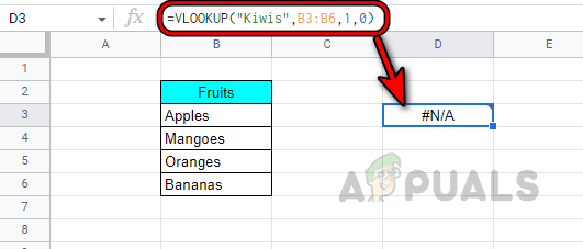
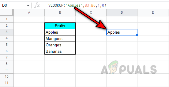
You can use a similar approach to clear #N/A errors on your Google sheet.
2. #Div/0 Error
Divided by zero is donated as #Div/O in Google Sheets. If any step in your formula divides a value by zero or an empty cell, then that would result in a #Dive/0 error. Let’s clear it by the following example:
- A #/Div/0 error in the cell D3 in the sheet below which has 3 columns: Numbers, Divided by, and Result:

#Div Error on a Google Sheet - As the formula in D3 implies that the value in B3 (that is 25) should be divided by the value in C3 (that is zero), so, the formula is asking Google Sheets to perform 25/0, which is mathematically impossible, so the #Div error.

Divided By Zero Causing #Div Error - Now, this error can be cleared by removing zero from the divisor (here, cell C3) or if that is not possible, then either leave the formula as it is (if not used in another calculation) or mask the result by using the IFERROR function.
- In the given example, let us mask the #Div/0 as the Wrong Division by using IFERROR. The general syntax of IFERROR is as under:
=IFERROR(value, (value_if_error))
- In our example, the formula would be:
=IFERROR("Wrong Division",(B3/C3))
Use the IFERROR Function to Mask a N/A Error on A Google Sheet - Now you can see that the result in the D3 cell has changed to Wrong Division.
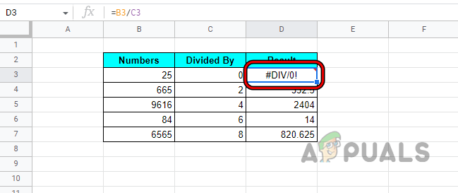
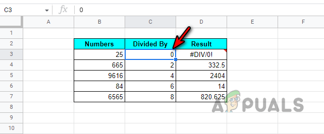
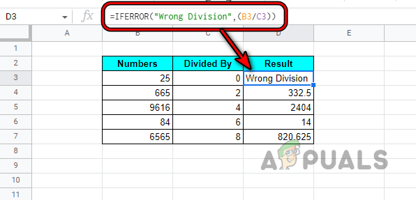
3. #Value Error
You may face a #value error on a Google sheet if the data type of at least a cell does not match what is required for the calculations to happen on a particular formula. In other words, a Google Sheet might show a #value error if you try to calculate a single data type (like a number) from two different input data types (like a number and a text string). Let us clear it by an example.
- Look at the sheet in the image below and you will notice a #value error the cell D3, although, other cells’ results are calculated correctly.

#Value Error on a Google Sheet - Then carefully inspect the formula and you will notice that cell D3 is a result of the addition of the value in cell B3 (that is 25) to the value of cell C3 (that is zero).

#Value Error Due to Summing a Text String with a Number - But zero is not a number but a text string, thus the Google Sheets fail to add a string to a number (different data types) and shows the #value error.
- Now, either you change the formula or change the value in the C3 cell from zero (text string) to 0 (numeric) as shown below:

Changing Zero Text to Numeric Zero Clears the #Value Error
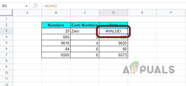
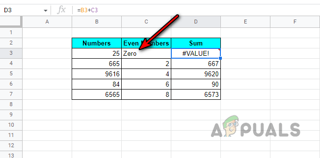
4. #Name Error
A Google Sheet might show the #name error if a function name is misspelled, quotation marks are not present in the formula syntax (if required), or a cell/range name is not correct. We have a very detailed article on our website about #name errors, do not forget to check it.
- Reference to the sheet in the image below and you will notice a #name error in cell D3.

#Name Error on the Google Sheet - The D3 cell combines the values of B3 and C3.
- Our cell references (B3 and C3) are valid and do not have a typo, now have a good look at the formula in D3, you will notice that the formula is:
=CONCATT(B3,C3)

Concatt is Not a Valid Function of a Google Sheet - Whereas CONCATT (an extra T added to the correct CONCAT) is not a valid formula, it should have been:
=CONCAT(B3,C3)
- Now see the image below where the #name error is cleared after correcting the CONCAT formula.

#Name Error Cleared After Correcting the Concat Formula
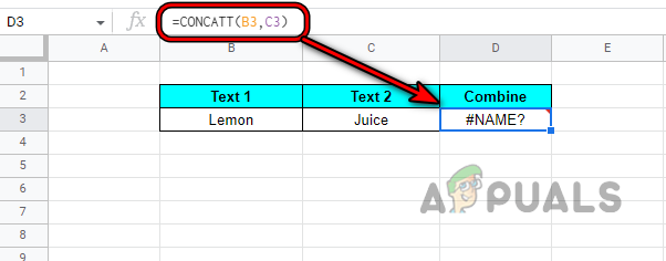
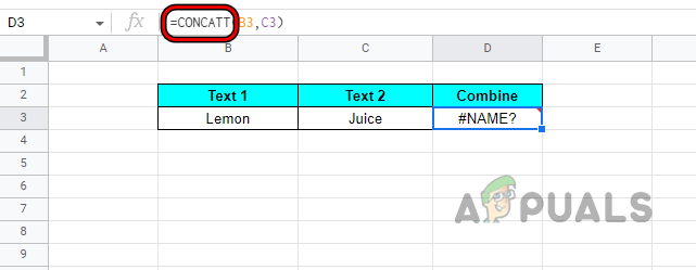
Let us take another example to clarify the idea about the #name error due to values.
- Reference to the sheet in the image below and you will notice a #name error in cell B3.
- Now have a good look at the formula and doesn’t everything look fine? Spellings of the CONCAT function are correct, lemon, and juice are also correct. Then what is causing the #name error?

#Name Error Even Formula and Value are Correct - Lemon and juice are text strings and as per Google Sheets syntax, these should be wrapped in double quotes, as you can see in the image below that after adding quotes around lemon and juice, the #name error is cleared from cell B3.

#Name Error Cleared After Adding Double-Quotes Around the Text Strings
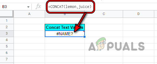
5. #Num Error
You may encounter the #num error on a Google sheet if the result of a calculation is larger than the maximum display capacity of Google Sheets i.e., 1.79769e+308. For example, if we multiply fifty-five billion by fourteen billion in a Google Sheet cell, then that will cause a #num error as Google Sheets cannot display such a large number. Another reason for this error is that the input type of a number does not meet the required type of the number type. Let us discuss it through an example:
- Refer to the sheet in the image below and you will notice a #num error in C7.

#Num Error on a Google Sheet - Now check the formula and you will notice that column C is the square root of column B.
- Then check cell B7 and you will find that it is a negative number but in basic mathematics, the square root of a positive number can be calculated only, thus Google Sheets throw a #name error.

Square Root of A Negative Number Causing the #Num Error on A Google Sheet - You can correct this either by changing the value (you can use the ABS function to convert the number to positive), formula, or hiding the result by using IFERROR (as discussed earlier).
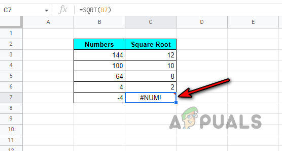
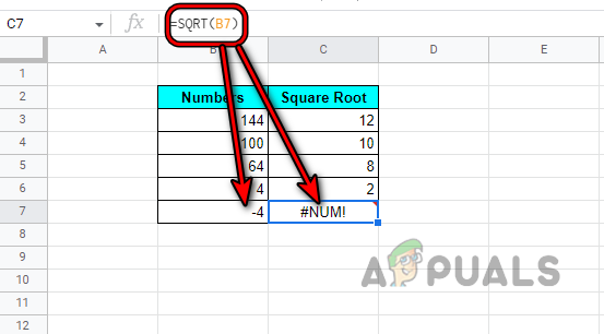
6. “#Error” Error
If a Google Sheet cannot understand a particular formula but cannot specify the reason for the error (like other errors where we get a hint like in #num error we know that the problem is with numbers), then that could result in a “#error” error. As the reason for the error is not specified, it is a more general error in nature or we can say that if a Google Sheet cannot link an error to any other error types of the parse error, then it will show a “#error” error. It could be a result of missing characters like commas, apostrophes, values, and parameters. Let us understand it with the following example:
- Look at the sheet in the image below and you will notice a “#error error” in cell D11.
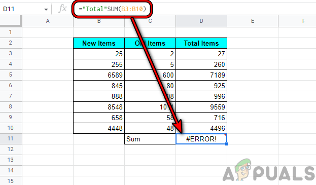
- Now have a good look at the formula in D11 and you will notice it is as under (as we are trying to sum the sums):
="Total"SUM(B3:B10)

A Wrong Sum Formula Caused #Error Error on a Google Sheet - But the total sum is not a valid function and we will only need a Sum Function to sum the sums like:
=SUM(B3:B10)
- Now check the sheet below after making the above amendment that clears the #error error:

#Error Cleared After Correcting the SUM Formula in a Google Sheet
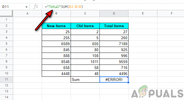
As this error is general, here are some steps that you may take to clear this type of parse error:
- Make sure the opening and closing parentheses in a formula match according to the amount required.
- If special characters such as the colons, semicolons, commas, and apostrophes are placed properly (if required by the formula).
- If the data contains dollar or percentage signs, make sure they are not part of your formula. Ensure those are input as normal numbers. If you are in a requirement to use these signs, then format the results as currencies (like Dollar) or percentages, not the inputs.
7. #Ref Error
This error might occur on a Google Sheet if the cell references used in the formula are not valid or missing. This error can mainly occur due to the followings:
- Deleted Cell References
- Circular Dependency
- Cell Reference Out of the Data Range
#Ref Error Due to Deleted Cell References
If a formula is referring to a cell range but that cell range is deleted, then it will cause a #ref error in the formula cell. Let us discuss an example in this regard:
- Refer to the image below and you will see a Sum column is set up in cells D3 to D7 that is adding columns B and C.

Sum Formula in the D Column - Now, we delete column C and that will cause a #ref error in column D as column C is deleted, which is part of the formula, thus #ref error.

#Ref Error After Deleting a Column on a Google Sheet - Here, either un-delete column C or amend the formula to remove references to deleted cells.
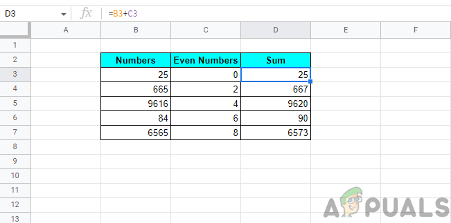
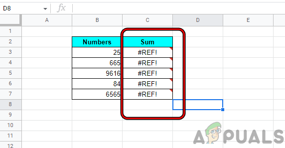
#Ref Error Due to Circular Dependency
If a formula cell is referring to itself as an input range, then that will cause a #ref error due to circular dependency. Let us clarify the concept by the following example:
- Reference to the sheet in the image below and you will notice a #ref error in cell B11.

#Ref Error on a Google Sheet - Now look to the formula in the cell B11:
=SUM(B2:B11)

#Ref Error Due to Circular Dependency - Then you will notice that the B11 cell is also referred to in the range and is also an input cell to itself, so #ref error due to the circular dependency.
- In this case, edit the formula to remove the cell from the referred range which clears the #ref error from B11:
=SUM(B2:B10)

#Name Cleared After Removing the Circular Dependency in the Formula

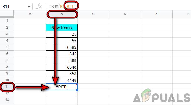
#Ref Error Due to Cell Reference Out of the Data Range
If you are using a function (like VLOOKUP) to search/extract an entry in a selected cell range but the cell reference given is outside the selected range, thus a #REF! error due to cell reference being out of the data range. Let’s discuss it through an example:
- Refer to the sheet shown in the image below and you will notice a #ref error in cell F4.

#Ref Error in the VLOOKUP Formula on A Google Sheet - Now look at the formula and you will find that it is referring to the 3rd column in the range (B3 to C7), whereas, the range has only two columns (B and C), thus #ref error due to cell reference out of the data range.

#Ref Error Due to Referring to a Column That is Not Present in the Range - Then edit the formula to use the 2nd column (the price column) and thus that clears the #ref error.

#Ref Error Due to Due to Cell Reference Out of the Data Range Cleared After Changing the Formula to Use Correct Column
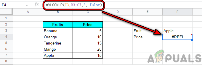
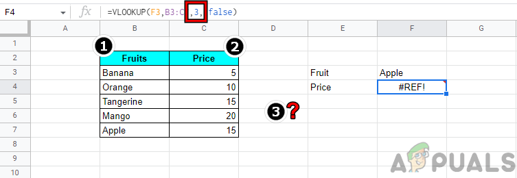
8. There Was a Problem Pop Up
This is probably the most recurring type of parse error. When this error occurs, you cannot do anything on the sheet till you fix or skip the formula. This error mostly occurs if a character is missing from the formula’s syntax or an extra character is present in the formula syntax. You can understand it by the following example:
- Refer to the sheet displayed in the image below and you will notice that There Was a Problem Pop Up shown when adding a sum formula in the cell B11:

There Was a Problem Error on A Google Sheet - Now you will notice that there is an extra / at the end of the formula and thus causing the parse error under discussion.
There Was a Problem Error on A Google Sheet - Then remove the / from the formula and that will clear the error:

There Was a Problem Error Cleared on the Google Sheet After Removing Slash From the End of the Formula
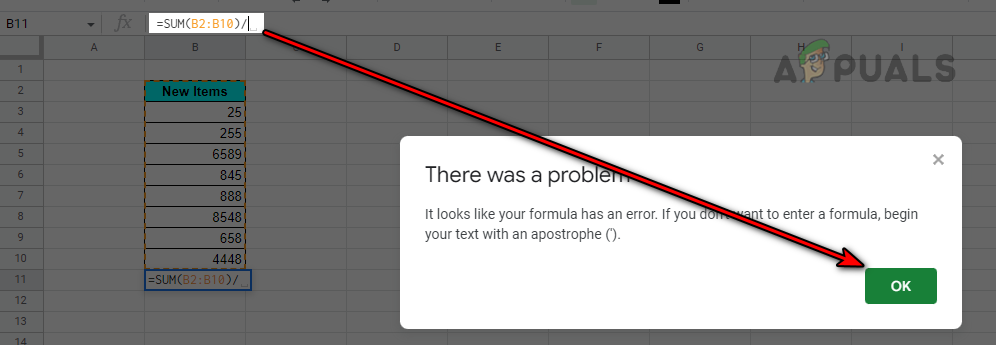
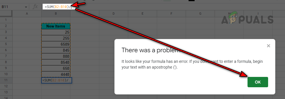
9. #Null Error
This error mainly occurs in Excel and if you copy the data from an Excel sheet to a Google sheet, then that may show a #null error. If an Excel sheet is uploaded to Google Sheets, then that data may show the
#error” error, not the #null error. Then either you clear the #null error in Excel or clear the “#error” error on Google Sheets (discussed earlier).
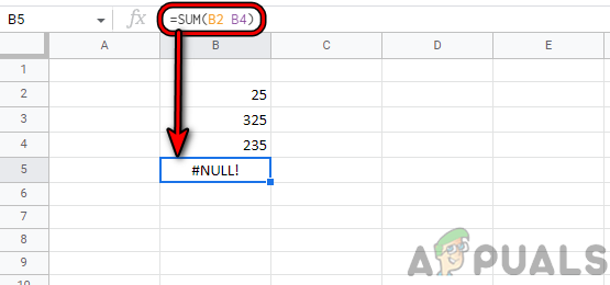
Functions to Deal Errors on a Large Google Sheet
As the above examples were simple to make the idea clear but on a large sheet, it becomes troublesome to find and troubleshoot errors. We are listing down some Google Sheet functions that make this process easier.
ISNA Function
You can use this function to check the selected cell range for a N/A error. It uses the following syntax:
=ISNA(value)
ISERR Function
If you are interested in all others errors in a range except the #N/A error, then this function will list down all such errors. Following is the syntax of this function:
=ISERR(value)
The ERROR TYPE Function
This Google Sheets function lists down every error on a sheet in numbers. It takes the following syntax:
=ERROR.TYPE(value)
The errors detected and the corresponding numbers are as followings:
#NULL!=1

#DIV/0!=2

#Value=3

#Ref=4

#NAME?=5

#NUM!=6

#N/A!=7

All other random errors on a Google sheet=8
If Error Function
If a parse error cannot be rectified due to circumstances, then you may hide it by using the IFERROR function, if no other calculations are getting disturbed. Please use it as a last resort because it can cause unintended issues in the future. You can refer to the #Div/0 Error section to understand the process.
Best Practices to Avoid a Parse Error
It is always better to avoid an error than to waste countless hours troubleshooting it. Here are some of the best practices that you can use to avoid parse errors.
- Make sure not to use symbols like % or $ in a formula.
- Punctuation marks in a formula are changed as per your region and language in a Google Sheet, so, if you are facing a parse error in a Google sheet, you may switch between commas to semicolons or vice versa to clear the error. In some regions, you may have to use instead of commas or semicolons.
- Keep in mind that you must write a formula in Google Sheets in English, even If you are using Google Sheets in a non-English language like French.
- Make sure your Locale in Spreadsheet Settings of Google Sheets and Time Zone are set to the same place as the United States, not like Locale set to the United States, and Time Zone set to Moscow.

Set Locale and Time Zone of A Google Sheet to the Same Place - If a parse error occurs on a Google Sheet, do not forget to check for the placement of quotes around text, links, image sources, etc. Also, keep an eye on when to use single quotes and when to use double quotes.
- When referring to a cell in another sheet in a formula, make sure to select the required cell on that sheet, not type it as it can sometimes return a parse error.
- Do note that when a plus sign and comma are used in a formula (this can happen when dealing with phone numbers) like the following, it will return a parse error on a Google Sheet.
+123,456                     // This will result in an error

+123456                      // This will not result in an error
- When copying or referring to whole columns or rows on a sheet from another sheet, always start with the 1st column or row, otherwise, mismatching rows and columns between the source and destination sheets will cause a parse error.
- Last, but not least, here is the link to a Google Sheet (without any Macros, add-ons, etc. but you must copy the sheet to your Google Sheets). This is an automated tool built as Evaluate Formula Parser (Google Sheets does not have one, whereas, Excel is equipped with it). This sheet can be used to evaluate a formula that is showing a parse error. You must use this sheet at your own risk and we will not be responsible for any issues caused by this sheet.
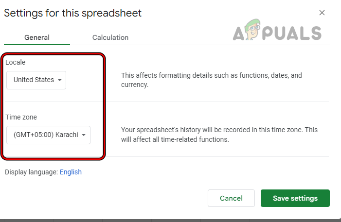
Hopefully, we have succeeded in clearing the parse errors on your Google sheet. If you have any queries or suggestions, you are more than welcome in the comments section.
Google Sheets is a powerful tool that comes with a ton of built-in functions that can be used to do many things.
As you work with spreadsheet programs like Google Sheets, eventually you will encounter a formula parse error. These errors can be pretty annoying, but eventually, with enough practice, you can learn to understand what these errors mean, and how to fix them.
In this tutorial, I am going to cover the common types of formula parse errors in Google Sheets and show you how to fix them.
Table of Contents
- 1 What is a Formula Parse Error?
- 2 There Was a Problem Popup
- 3 #N/A Error
- 4 #VALUE! Error
- 5 #DIV/0 Error
- 6 #REF! Error
- 7 #ERROR! Error
- 8 #NAME? Error
- 9 #NUM! Error
- 10 Closing Thoughts
What is a Formula Parse Error?
A formula parse error is an error that is returned when Google Sheets does not understand your formula. The formula isn’t working properly and so you are returned an error message.
There are many different things that can cause these errors.
Some common reasons include:
- A typo in the formula
- Missing arguments or too many arguments in a function
- Mathematically impossible calculations
- Cell reference issues
Understanding why your formula is returning an error is important. Below I will cover the different types of error messages, what they mean, and how to resolve them.
One common type of error message that you may receive when entering a formula in Google Sheets is the “There was a problem” popup.
This popup will say something like this: “It looks like your formula has an error. If you don’t want to enter a formula, begin your text with an apostrophe (‘).”

This error usually occurs when there is a problem with the formula. Usually, it means there is a character in the formula that shouldn’t be.
If you get this error message, it is likely that you mistyped and have some kind of character in the formula that should be removed.
To fix this, double-check that your formula doesn’t have anything that shouldn’t be there:

Once you remove the unwanted character, the formula should work as normal.
#N/A Error
The #N/A error occurs when a value that the formula needs is not available. It most often occurs if you’re using a lookup function and it cannot find the value that you are looking for.

You can see in the example above, I have a lookup function searching in cells A1:B4.
As you may notice, the very last value in my lookup does not exist in that cell range, so that formula results in an #N/A error message.
The only way to fix this error message is to make sure that the value you are searching for is available wherever you are searching, so double-check and make sure your data ranges are correct. If the value really doesn’t exist, you can hide the error message with a function like IFERROR.
#VALUE! Error
The #VALUE! error will occur when the data type that a formula expects is wrong. For example, if you are trying to do math operations with a text value, this error will occur. Because Google Sheets is expecting number values.

You can see in the example above I have the wrong cell in my formula and it is set to add cells A1+B2 together. Cell A1 is a text value you though, so the #VALUE! error is returned.
This error message can also occur if you have a space in a cell.
If you get this error message, pay attention to the wording of the message that is returned.
In the above example, the error says “Function ADD parameter 1 expects number values“.
This is a great hint that the value that is the problem is the first parameter in my formula.
So to fix this, check and make sure every input into the formula is the correct kind of data, and make sure to read the error message for clues on what is causing the issue.
#DIV/0 Error
The #DIV/0 error message will return if you try to divide by 0 or divide by a blank cell. This is mathematically impossible, so the formula will always result in this formula parse error.

To fix this error, check the parameters used in your argument and make sure none of them is zero or blank.
If they are zero or blank, the only real solution that you will have is to either not use the formula or hide the error message with IFERROR.
#REF! Error
The #REF! error will return when you have a reference that is invalid.
A common issue that causes this error is that formula was set up on a row or column that has been deleted.

Another common reason this error may return is that you are trying to reference a cell that is outside of a data range.

In the example above, I have a lookup function searching columns A:B that is trying to return a value in column 3. However, A:B is only 2 columns, so my formula is trying to lookup out of bounds. This will cause a #REF! error.
Another reason you may get this error is that there could be a circular dependency detected in one of your formulas.

You can see in the example above, there is a circular dependency detected. This is because the formula for column K2 depends on the value column L2 and the formula for column L2 depends on the value in column K2. This will cause an error.
To fix a #REF! error, you need to diagnose what is causing your error.
Check your formulas and make sure the cell range is not out of bounds. If it is out of bounds, fix your formula so that it is only searching for in-bound cells.
Make sure that the cells that the formulas were set up on initially have not accidentally been deleted. If they have been deleted you will have to set up your formula again on a new cell.
If it is a circular dependency that is causing your error, make sure that you do not have formulas that depend on the value of each other.
The #ERROR! formula parse error will occur in Google Sheets when the formula that you have entered is not being understood.
This could be caused by a few different things, from extra or missing parenthesis, extra or missing quotation marks, or other mistakes in your formula.

In the example above, there are extra quotation marks outside the formula and this is causing Google Sheets to not understand the formula which results in the #ERROR! message.
Whenever you get this error message, you need to check your formula and make sure it is set up properly.
#NAME? Error
The #NAME? the error will occur if there is a problem with the syntax of your formula.
It most often occurs if you have misspelled the name of one of the functions.

You can see in the example above the #NAME? error is returning a message stating “unknown function”.
You can also get this error if you are trying to reference a named range that doesn’t exist, or if you are trying to perform a function like CONCATENATE and you forget to put quotation marks around your text values

To fix this error message, check the message that is being returned. If the function is misspelled, make sure you are using the correct spelling.
If it is missing quotation marks around your text values, make sure to add those, and if you have misspelled a named range, you will need to correct that.
#NUM! Error
If you are using a function and you have numeric values that are invalid for the function you are using, this will often return a #NUM! error.
The #NUM! error simply means that the numbers you are using aren’t valid.
For example, here I have a SQRT (square root) function set up on the number -1. But this function only works if the parameter is positive or zero, so it results in an error message.

To fix this error, double-check the function you are using and make sure all the parameters used in your formula are acceptable values for the function.
You will find that one of the numbers might not meet the requirements for the function.
Closing Thoughts
Having errors in your spreadsheet can be incredibly frustrating, but if you take the time to learn what each error means, and how to diagnose your formulas for issues, you should be able to fix most errors that you encounter.
Every once in a while you may come across an error that you really can’t figure out. At that point, you may want to check out some of the various help forums for getting help in Google Sheets.
More Google Sheets Tutorials:
How to Use the ISNA Function
FILTER Has Mismatched Range Sizes