
To clean up transmission errors introduced by Earth’s atmosphere (left), Goddard scientists applied Reed–Solomon error correction (right), which is commonly used in CDs and DVDs. Typical errors include missing pixels (white) and false signals (black). The white stripe indicates a brief period when transmission was interrupted.
In information theory and coding theory with applications in computer science and telecommunication, error detection and correction (EDAC) or error control are techniques that enable reliable delivery of digital data over unreliable communication channels. Many communication channels are subject to channel noise, and thus errors may be introduced during transmission from the source to a receiver. Error detection techniques allow detecting such errors, while error correction enables reconstruction of the original data in many cases.
Definitions[edit]
Error detection is the detection of errors caused by noise or other impairments during transmission from the transmitter to the receiver.
Error correction is the detection of errors and reconstruction of the original, error-free data.
History[edit]
In classical antiquity, copyists of the Hebrew Bible were paid for their work according to the number of stichs (lines of verse). As the prose books of the Bible were hardly ever written in stichs, the copyists, in order to estimate the amount of work, had to count the letters.[1] This also helped ensure accuracy in the transmission of the text with the production of subsequent copies.[2][3] Between the 7th and 10th centuries CE a group of Jewish scribes formalized and expanded this to create the Numerical Masorah to ensure accurate reproduction of the sacred text. It included counts of the number of words in a line, section, book and groups of books, noting the middle stich of a book, word use statistics, and commentary.[1] Standards became such that a deviation in even a single letter in a Torah scroll was considered unacceptable.[4] The effectiveness of their error correction method was verified by the accuracy of copying through the centuries demonstrated by discovery of the Dead Sea Scrolls in 1947–1956, dating from c.150 BCE-75 CE.[5]
The modern development of error correction codes is credited to Richard Hamming in 1947.[6] A description of Hamming’s code appeared in Claude Shannon’s A Mathematical Theory of Communication[7] and was quickly generalized by Marcel J. E. Golay.[8]
Introduction[edit]
All error-detection and correction schemes add some redundancy (i.e., some extra data) to a message, which receivers can use to check consistency of the delivered message, and to recover data that has been determined to be corrupted. Error-detection and correction schemes can be either systematic or non-systematic. In a systematic scheme, the transmitter sends the original data, and attaches a fixed number of check bits (or parity data), which are derived from the data bits by some deterministic algorithm. If only error detection is required, a receiver can simply apply the same algorithm to the received data bits and compare its output with the received check bits; if the values do not match, an error has occurred at some point during the transmission. In a system that uses a non-systematic code, the original message is transformed into an encoded message carrying the same information and that has at least as many bits as the original message.
Good error control performance requires the scheme to be selected based on the characteristics of the communication channel. Common channel models include memoryless models where errors occur randomly and with a certain probability, and dynamic models where errors occur primarily in bursts. Consequently, error-detecting and correcting codes can be generally distinguished between random-error-detecting/correcting and burst-error-detecting/correcting. Some codes can also be suitable for a mixture of random errors and burst errors.
If the channel characteristics cannot be determined, or are highly variable, an error-detection scheme may be combined with a system for retransmissions of erroneous data. This is known as automatic repeat request (ARQ), and is most notably used in the Internet. An alternate approach for error control is hybrid automatic repeat request (HARQ), which is a combination of ARQ and error-correction coding.
Types of error correction[edit]
There are three major types of error correction.[9]
Automatic repeat request[edit]
Automatic repeat request (ARQ) is an error control method for data transmission that makes use of error-detection codes, acknowledgment and/or negative acknowledgment messages, and timeouts to achieve reliable data transmission. An acknowledgment is a message sent by the receiver to indicate that it has correctly received a data frame.
Usually, when the transmitter does not receive the acknowledgment before the timeout occurs (i.e., within a reasonable amount of time after sending the data frame), it retransmits the frame until it is either correctly received or the error persists beyond a predetermined number of retransmissions.
Three types of ARQ protocols are Stop-and-wait ARQ, Go-Back-N ARQ, and Selective Repeat ARQ.
ARQ is appropriate if the communication channel has varying or unknown capacity, such as is the case on the Internet. However, ARQ requires the availability of a back channel, results in possibly increased latency due to retransmissions, and requires the maintenance of buffers and timers for retransmissions, which in the case of network congestion can put a strain on the server and overall network capacity.[10]
For example, ARQ is used on shortwave radio data links in the form of ARQ-E, or combined with multiplexing as ARQ-M.
Forward error correction[edit]
Forward error correction (FEC) is a process of adding redundant data such as an error-correcting code (ECC) to a message so that it can be recovered by a receiver even when a number of errors (up to the capability of the code being used) are introduced, either during the process of transmission or on storage. Since the receiver does not have to ask the sender for retransmission of the data, a backchannel is not required in forward error correction. Error-correcting codes are used in lower-layer communication such as cellular network, high-speed fiber-optic communication and Wi-Fi,[11][12] as well as for reliable storage in media such as flash memory, hard disk and RAM.[13]
Error-correcting codes are usually distinguished between convolutional codes and block codes:
- Convolutional codes are processed on a bit-by-bit basis. They are particularly suitable for implementation in hardware, and the Viterbi decoder allows optimal decoding.
- Block codes are processed on a block-by-block basis. Early examples of block codes are repetition codes, Hamming codes and multidimensional parity-check codes. They were followed by a number of efficient codes, Reed–Solomon codes being the most notable due to their current widespread use. Turbo codes and low-density parity-check codes (LDPC) are relatively new constructions that can provide almost optimal efficiency.
Shannon’s theorem is an important theorem in forward error correction, and describes the maximum information rate at which reliable communication is possible over a channel that has a certain error probability or signal-to-noise ratio (SNR). This strict upper limit is expressed in terms of the channel capacity. More specifically, the theorem says that there exist codes such that with increasing encoding length the probability of error on a discrete memoryless channel can be made arbitrarily small, provided that the code rate is smaller than the channel capacity. The code rate is defined as the fraction k/n of k source symbols and n encoded symbols.
The actual maximum code rate allowed depends on the error-correcting code used, and may be lower. This is because Shannon’s proof was only of existential nature, and did not show how to construct codes which are both optimal and have efficient encoding and decoding algorithms.
Hybrid schemes[edit]
Hybrid ARQ is a combination of ARQ and forward error correction. There are two basic approaches:[10]
- Messages are always transmitted with FEC parity data (and error-detection redundancy). A receiver decodes a message using the parity information, and requests retransmission using ARQ only if the parity data was not sufficient for successful decoding (identified through a failed integrity check).
- Messages are transmitted without parity data (only with error-detection information). If a receiver detects an error, it requests FEC information from the transmitter using ARQ, and uses it to reconstruct the original message.
The latter approach is particularly attractive on an erasure channel when using a rateless erasure code.
Error detection schemes[edit]
Error detection is most commonly realized using a suitable hash function (or specifically, a checksum, cyclic redundancy check or other algorithm). A hash function adds a fixed-length tag to a message, which enables receivers to verify the delivered message by recomputing the tag and comparing it with the one provided.
There exists a vast variety of different hash function designs. However, some are of particularly widespread use because of either their simplicity or their suitability for detecting certain kinds of errors (e.g., the cyclic redundancy check’s performance in detecting burst errors).
Minimum distance coding[edit]
A random-error-correcting code based on minimum distance coding can provide a strict guarantee on the number of detectable errors, but it may not protect against a preimage attack.
Repetition codes[edit]
A repetition code is a coding scheme that repeats the bits across a channel to achieve error-free communication. Given a stream of data to be transmitted, the data are divided into blocks of bits. Each block is transmitted some predetermined number of times. For example, to send the bit pattern «1011», the four-bit block can be repeated three times, thus producing «1011 1011 1011». If this twelve-bit pattern was received as «1010 1011 1011» – where the first block is unlike the other two – an error has occurred.
A repetition code is very inefficient, and can be susceptible to problems if the error occurs in exactly the same place for each group (e.g., «1010 1010 1010» in the previous example would be detected as correct). The advantage of repetition codes is that they are extremely simple, and are in fact used in some transmissions of numbers stations.[14][15]
Parity bit[edit]
A parity bit is a bit that is added to a group of source bits to ensure that the number of set bits (i.e., bits with value 1) in the outcome is even or odd. It is a very simple scheme that can be used to detect single or any other odd number (i.e., three, five, etc.) of errors in the output. An even number of flipped bits will make the parity bit appear correct even though the data is erroneous.
Parity bits added to each «word» sent are called transverse redundancy checks, while those added at the end of a stream of «words» are called longitudinal redundancy checks. For example, if each of a series of m-bit «words» has a parity bit added, showing whether there were an odd or even number of ones in that word, any word with a single error in it will be detected. It will not be known where in the word the error is, however. If, in addition, after each stream of n words a parity sum is sent, each bit of which shows whether there were an odd or even number of ones at that bit-position sent in the most recent group, the exact position of the error can be determined and the error corrected. This method is only guaranteed to be effective, however, if there are no more than 1 error in every group of n words. With more error correction bits, more errors can be detected and in some cases corrected.
There are also other bit-grouping techniques.
Checksum[edit]
A checksum of a message is a modular arithmetic sum of message code words of a fixed word length (e.g., byte values). The sum may be negated by means of a ones’-complement operation prior to transmission to detect unintentional all-zero messages.
Checksum schemes include parity bits, check digits, and longitudinal redundancy checks. Some checksum schemes, such as the Damm algorithm, the Luhn algorithm, and the Verhoeff algorithm, are specifically designed to detect errors commonly introduced by humans in writing down or remembering identification numbers.
Cyclic redundancy check[edit]
A cyclic redundancy check (CRC) is a non-secure hash function designed to detect accidental changes to digital data in computer networks. It is not suitable for detecting maliciously introduced errors. It is characterized by specification of a generator polynomial, which is used as the divisor in a polynomial long division over a finite field, taking the input data as the dividend. The remainder becomes the result.
A CRC has properties that make it well suited for detecting burst errors. CRCs are particularly easy to implement in hardware and are therefore commonly used in computer networks and storage devices such as hard disk drives.
The parity bit can be seen as a special-case 1-bit CRC.
Cryptographic hash function[edit]
The output of a cryptographic hash function, also known as a message digest, can provide strong assurances about data integrity, whether changes of the data are accidental (e.g., due to transmission errors) or maliciously introduced. Any modification to the data will likely be detected through a mismatching hash value. Furthermore, given some hash value, it is typically infeasible to find some input data (other than the one given) that will yield the same hash value. If an attacker can change not only the message but also the hash value, then a keyed hash or message authentication code (MAC) can be used for additional security. Without knowing the key, it is not possible for the attacker to easily or conveniently calculate the correct keyed hash value for a modified message.
Error correction code[edit]
Any error-correcting code can be used for error detection. A code with minimum Hamming distance, d, can detect up to d − 1 errors in a code word. Using minimum-distance-based error-correcting codes for error detection can be suitable if a strict limit on the minimum number of errors to be detected is desired.
Codes with minimum Hamming distance d = 2 are degenerate cases of error-correcting codes, and can be used to detect single errors. The parity bit is an example of a single-error-detecting code.
Applications[edit]
Applications that require low latency (such as telephone conversations) cannot use automatic repeat request (ARQ); they must use forward error correction (FEC). By the time an ARQ system discovers an error and re-transmits it, the re-sent data will arrive too late to be usable.
Applications where the transmitter immediately forgets the information as soon as it is sent (such as most television cameras) cannot use ARQ; they must use FEC because when an error occurs, the original data is no longer available.
Applications that use ARQ must have a return channel; applications having no return channel cannot use ARQ.
Applications that require extremely low error rates (such as digital money transfers) must use ARQ due to the possibility of uncorrectable errors with FEC.
Reliability and inspection engineering also make use of the theory of error-correcting codes.[16]
Internet[edit]
In a typical TCP/IP stack, error control is performed at multiple levels:
- Each Ethernet frame uses CRC-32 error detection. Frames with detected errors are discarded by the receiver hardware.
- The IPv4 header contains a checksum protecting the contents of the header. Packets with incorrect checksums are dropped within the network or at the receiver.
- The checksum was omitted from the IPv6 header in order to minimize processing costs in network routing and because current link layer technology is assumed to provide sufficient error detection (see also RFC 3819).
- UDP has an optional checksum covering the payload and addressing information in the UDP and IP headers. Packets with incorrect checksums are discarded by the network stack. The checksum is optional under IPv4, and required under IPv6. When omitted, it is assumed the data-link layer provides the desired level of error protection.
- TCP provides a checksum for protecting the payload and addressing information in the TCP and IP headers. Packets with incorrect checksums are discarded by the network stack, and eventually get retransmitted using ARQ, either explicitly (such as through three-way handshake) or implicitly due to a timeout.
Deep-space telecommunications[edit]
The development of error-correction codes was tightly coupled with the history of deep-space missions due to the extreme dilution of signal power over interplanetary distances, and the limited power availability aboard space probes. Whereas early missions sent their data uncoded, starting in 1968, digital error correction was implemented in the form of (sub-optimally decoded) convolutional codes and Reed–Muller codes.[17] The Reed–Muller code was well suited to the noise the spacecraft was subject to (approximately matching a bell curve), and was implemented for the Mariner spacecraft and used on missions between 1969 and 1977.
The Voyager 1 and Voyager 2 missions, which started in 1977, were designed to deliver color imaging and scientific information from Jupiter and Saturn.[18] This resulted in increased coding requirements, and thus, the spacecraft were supported by (optimally Viterbi-decoded) convolutional codes that could be concatenated with an outer Golay (24,12,8) code. The Voyager 2 craft additionally supported an implementation of a Reed–Solomon code. The concatenated Reed–Solomon–Viterbi (RSV) code allowed for very powerful error correction, and enabled the spacecraft’s extended journey to Uranus and Neptune. After ECC system upgrades in 1989, both crafts used V2 RSV coding.
The Consultative Committee for Space Data Systems currently recommends usage of error correction codes with performance similar to the Voyager 2 RSV code as a minimum. Concatenated codes are increasingly falling out of favor with space missions, and are replaced by more powerful codes such as Turbo codes or LDPC codes.
The different kinds of deep space and orbital missions that are conducted suggest that trying to find a one-size-fits-all error correction system will be an ongoing problem. For missions close to Earth, the nature of the noise in the communication channel is different from that which a spacecraft on an interplanetary mission experiences. Additionally, as a spacecraft increases its distance from Earth, the problem of correcting for noise becomes more difficult.
Satellite broadcasting[edit]
The demand for satellite transponder bandwidth continues to grow, fueled by the desire to deliver television (including new channels and high-definition television) and IP data. Transponder availability and bandwidth constraints have limited this growth. Transponder capacity is determined by the selected modulation scheme and the proportion of capacity consumed by FEC.
Data storage[edit]
Error detection and correction codes are often used to improve the reliability of data storage media.[19] A parity track capable of detecting single-bit errors was present on the first magnetic tape data storage in 1951. The optimal rectangular code used in group coded recording tapes not only detects but also corrects single-bit errors. Some file formats, particularly archive formats, include a checksum (most often CRC32) to detect corruption and truncation and can employ redundancy or parity files to recover portions of corrupted data. Reed-Solomon codes are used in compact discs to correct errors caused by scratches.
Modern hard drives use Reed–Solomon codes to detect and correct minor errors in sector reads, and to recover corrupted data from failing sectors and store that data in the spare sectors.[20] RAID systems use a variety of error correction techniques to recover data when a hard drive completely fails. Filesystems such as ZFS or Btrfs, as well as some RAID implementations, support data scrubbing and resilvering, which allows bad blocks to be detected and (hopefully) recovered before they are used.[21] The recovered data may be re-written to exactly the same physical location, to spare blocks elsewhere on the same piece of hardware, or the data may be rewritten onto replacement hardware.
Error-correcting memory[edit]
Dynamic random-access memory (DRAM) may provide stronger protection against soft errors by relying on error-correcting codes. Such error-correcting memory, known as ECC or EDAC-protected memory, is particularly desirable for mission-critical applications, such as scientific computing, financial, medical, etc. as well as extraterrestrial applications due to the increased radiation in space.
Error-correcting memory controllers traditionally use Hamming codes, although some use triple modular redundancy. Interleaving allows distributing the effect of a single cosmic ray potentially upsetting multiple physically neighboring bits across multiple words by associating neighboring bits to different words. As long as a single-event upset (SEU) does not exceed the error threshold (e.g., a single error) in any particular word between accesses, it can be corrected (e.g., by a single-bit error-correcting code), and the illusion of an error-free memory system may be maintained.[22]
In addition to hardware providing features required for ECC memory to operate, operating systems usually contain related reporting facilities that are used to provide notifications when soft errors are transparently recovered. One example is the Linux kernel’s EDAC subsystem (previously known as Bluesmoke), which collects the data from error-checking-enabled components inside a computer system; besides collecting and reporting back the events related to ECC memory, it also supports other checksumming errors, including those detected on the PCI bus.[23][24][25] A few systems[specify] also support memory scrubbing to catch and correct errors early before they become unrecoverable.
See also[edit]
- Berger code
- Burst error-correcting code
- ECC memory, a type of computer data storage
- Link adaptation
- List of algorithms § Error detection and correction
- List of hash functions
References[edit]
- ^ a b «Masorah». Jewish Encyclopedia.
- ^ Pratico, Gary D.; Pelt, Miles V. Van (2009). Basics of Biblical Hebrew Grammar: Second Edition. Zondervan. ISBN 978-0-310-55882-8.
- ^ Mounce, William D. (2007). Greek for the Rest of Us: Using Greek Tools Without Mastering Biblical Languages. Zondervan. p. 289. ISBN 978-0-310-28289-1.
- ^ Mishneh Torah, Tefillin, Mezuzah, and Sefer Torah, 1:2. Example English translation: Eliyahu Touger. The Rambam’s Mishneh Torah. Moznaim Publishing Corporation.
- ^ Brian M. Fagan (5 December 1996). «Dead Sea Scrolls». The Oxford Companion to Archaeology. Oxford University Press. ISBN 0195076184.
- ^ Thompson, Thomas M. (1983), From Error-Correcting Codes through Sphere Packings to Simple Groups, The Carus Mathematical Monographs (#21), The Mathematical Association of America, p. vii, ISBN 0-88385-023-0
- ^ Shannon, C.E. (1948), «A Mathematical Theory of Communication», Bell System Technical Journal, 27 (3): 379–423, doi:10.1002/j.1538-7305.1948.tb01338.x, hdl:10338.dmlcz/101429, PMID 9230594
- ^ Golay, Marcel J. E. (1949), «Notes on Digital Coding», Proc.I.R.E. (I.E.E.E.), 37: 657
- ^ Gupta, Vikas; Verma, Chanderkant (November 2012). «Error Detection and Correction: An Introduction». International Journal of Advanced Research in Computer Science and Software Engineering. 2 (11). S2CID 17499858.
- ^ a b A. J. McAuley, Reliable Broadband Communication Using a Burst Erasure Correcting Code, ACM SIGCOMM, 1990.
- ^ Shah, Pradeep M.; Vyavahare, Prakash D.; Jain, Anjana (September 2015). «Modern error correcting codes for 4G and beyond: Turbo codes and LDPC codes». 2015 Radio and Antenna Days of the Indian Ocean (RADIO): 1–2. doi:10.1109/RADIO.2015.7323369. ISBN 978-9-9903-7339-4. S2CID 28885076. Retrieved 22 May 2022.
- ^ «IEEE SA — IEEE 802.11ac-2013». IEEE Standards Association.
- ^ «Transition to Advanced Format 4K Sector Hard Drives | Seagate US». Seagate.com. Retrieved 22 May 2022.
- ^ Frank van Gerwen. «Numbers (and other mysterious) stations». Archived from the original on 12 July 2017. Retrieved 12 March 2012.
- ^ Gary Cutlack (25 August 2010). «Mysterious Russian ‘Numbers Station’ Changes Broadcast After 20 Years». Gizmodo. Retrieved 12 March 2012.
- ^ Ben-Gal I.; Herer Y.; Raz T. (2003). «Self-correcting inspection procedure under inspection errors» (PDF). IIE Transactions. IIE Transactions on Quality and Reliability, 34(6), pp. 529-540. Archived from the original (PDF) on 2013-10-13. Retrieved 2014-01-10.
- ^ K. Andrews et al., The Development of Turbo and LDPC Codes for Deep-Space Applications, Proceedings of the IEEE, Vol. 95, No. 11, Nov. 2007.
- ^ Huffman, William Cary; Pless, Vera S. (2003). Fundamentals of Error-Correcting Codes. Cambridge University Press. ISBN 978-0-521-78280-7.
- ^ Kurtas, Erozan M.; Vasic, Bane (2018-10-03). Advanced Error Control Techniques for Data Storage Systems. CRC Press. ISBN 978-1-4200-3649-7.[permanent dead link]
- ^ Scott A. Moulton. «My Hard Drive Died». Archived from the original on 2008-02-02.
- ^ Qiao, Zhi; Fu, Song; Chen, Hsing-Bung; Settlemyer, Bradley (2019). «Building Reliable High-Performance Storage Systems: An Empirical and Analytical Study». 2019 IEEE International Conference on Cluster Computing (CLUSTER): 1–10. doi:10.1109/CLUSTER.2019.8891006. ISBN 978-1-7281-4734-5. S2CID 207951690.
- ^ «Using StrongArm SA-1110 in the On-Board Computer of Nanosatellite». Tsinghua Space Center, Tsinghua University, Beijing. Archived from the original on 2011-10-02. Retrieved 2009-02-16.
- ^ Jeff Layton. «Error Detection and Correction». Linux Magazine. Retrieved 2014-08-12.
- ^ «EDAC Project». bluesmoke.sourceforge.net. Retrieved 2014-08-12.
- ^ «Documentation/edac.txt». Linux kernel documentation. kernel.org. 2014-06-16. Archived from the original on 2009-09-05. Retrieved 2014-08-12.
Further reading[edit]
- Shu Lin; Daniel J. Costello, Jr. (1983). Error Control Coding: Fundamentals and Applications. Prentice Hall. ISBN 0-13-283796-X.
- SoftECC: A System for Software Memory Integrity Checking
- A Tunable, Software-based DRAM Error Detection and Correction Library for HPC
- Detection and Correction of Silent Data Corruption for Large-Scale High-Performance Computing
External links[edit]
- The on-line textbook: Information Theory, Inference, and Learning Algorithms, by David J.C. MacKay, contains chapters on elementary error-correcting codes; on the theoretical limits of error-correction; and on the latest state-of-the-art error-correcting codes, including low-density parity-check codes, turbo codes, and fountain codes.
- ECC Page — implementations of popular ECC encoding and decoding routines
What is an Error?
Transmitted data can be corrupted during communication. It is likely to be affected by external noise or other physical failures. In such a situation, the input data can’t be the same as the output data. This mismatch is known as “Error.”
The data errors may result in the loss of important or secure data. Most of the data transfer in digital systems will be in the form of ‘Bit transfer.’ Even a small bit of change can affect the performance of the entire system. In a data sequence, if 1 is changed to 0 or 0 is changed to 1, it is called “Bit error.”
In this Hamming code tutorial, you will learn:
- What is an Error?
- Types of Errors
- What is Error Detection & Error Correction?
- What is a Hamming Code?
- History of Hamming Code
- Application of Hamming Code
- Advantages of Hamming Code
- Disadvantages of Hamming Code
- How to Encode a message in Hamming Code
- Decrypting a Message in Hamming Code
Types of Errors
There are mainly three types of a bit error that occur in data transmission from the sender to the receiver.
- Single bit errors
- Multiple bit errors
- Burst errors

Single Bit Errors
The change made in one bit in the entire data sequence is known as “Single bit error”. However, the occurrence of single-bit error is not that common. Moreover, this error only occurs in a parallel communication system because data is transferred bitwise in a single line. Therefore, there is more chances that a single line can be noisy.
Multiple Bit Errors
In data sequence, if there is a change in two or more bits of a data sequence of a transmitter to receiver, it is known as “Multiple bit errors.”
This type of error mostly occurs in both serial and parallel type data communication networks.
Burst Errors
The change of the set of bits in data sequence is known as “Burst error”. This type of data error is calculated in from the first-bit change to last bit change.
In digital communication system error will be transferred from one communication system into another. If these errors are not detected and corrected, then the data will be lost. For effective communication, system data should transfer with high accuracy. This will be done by first identifying the errors and them correcting them.
Error detection is a method of detecting the errors which are present in the data transmitted from a transmitter to receiver in a data communication system.
Here, you can use redundancy codes to find these errors, by adding to the data when it is transmitted from the source. These codes is called “Error detecting codes”.
Three types of error detection codes are:
- Parity Checking
- Cyclic Redundancy Check (CRC)
- Longitudinal Redundancy Check (LRC)
Parity Checking
- It is also known as a parity check.
- It has a cost-effective mechanism for error detection.
- In this technique, the redundant bit is known as a parity bit. It is appended for every data unit. The total number of 1s in the unit should become even, which is known as a parity bit.
Longitudinal Redundancy Check
In this error detection technique, a block of bits is organized in the tabular format. LRC method helps you to calculate the parity bit for every column. The set of this parity is also sent along with the original data. The block of parity helps you to check the redundancy.
Cyclic Redundancy Check
Cyclic Redundancy Check is a sequence of redundant that must be appended to the end of the unit. That’s why the resulting data unit should become divisible by a second, predetermined binary number.
At the destination, the incoming data needs to be divided by the same number. In case if there is no remainder, then the data unit is assumed to be correct and is accepted. Otherwise, it indicates that the data unit is damaged in transmission, and hence it must be rejected.
What is a Hamming code?
Hamming code is a liner code that is useful for error detection up to two immediate bit errors. It is capable of single-bit errors.
In Hamming code, the source encodes the message by adding redundant bits in the message. These redundant bits are mostly inserted and generated at certain positions in the message to accomplish error detection and correction process.
History of Hamming code
- Hamming code is a technique build by R.W.Hamming to detect errors.
- Hamming code should be applied to data units of any length and uses the relationship between data and redundancy bits.
- He worked on the problem of the error-correction method and developed an increasingly powerful array of algorithms called Hamming code.
- In 1950, he published the Hamming Code, which widely used today in applications like ECC memory.
Application of Hamming code
Here are some common applications of using Hamming code:
- Satellites
- Computer Memory
- Modems
- PlasmaCAM
- Open connectors
- Shielding wire
- Embedded Processor
Advantages of Hamming code
- Hamming code method is effective on networks where the data streams are given for the single-bit errors.
- Hamming code not only provides the detection of a bit error but also helps you to indent bit containing error so that it can be corrected.
- The ease of use of hamming codes makes it best them suitable for use in computer memory and single-error correction.
Disadvantages of Hamming code
- Single-bit error detection and correction code. However, if multiple bits are founded error, then the outcome may result in another bit which should be correct to be changed. This can cause the data to be further errored.
- Hamming code algorithm can solve only single bits issues.
How to Encode a message in Hamming Code
The process used by the sender to encode the message includes the following three steps:
- Calculation of total numbers of redundant bits.
- Checking the position of the redundant bits.
- Lastly, calculating the values of these redundant bits.
When the above redundant bits are embedded within the message, it is sent to the user.
Step 1) Calculation of the total number of redundant bits.
Let assume that the message contains:
- n– number of data bits
- p – number of redundant bits which are added to it so that np can indicate at least (n + p + 1) different states.
Here, (n + p) depicts the location of an error in each of (n + p) bit positions and one extra state indicates no error. As p bits can indicate 2p states, 2p has to at least equal to (n + p + 1).
Step 2) Placing the redundant bits in their correct position.
The p redundant bits should be placed at bit positions of powers of 2. For example, 1, 2, 4, 8, 16, etc. They are referred to as p1 (at position 1), p2 (at position 2), p3 (at position 4), etc.
Step 3) Calculation of the values of the redundant bit.
The redundant bits should be parity bits makes the number of 1s either even or odd.
The two types of parity are ?
- Total numbers of bits in the message is made even is called even parity.
- The total number of bits in the message is made odd is called odd parity.
Here, all the redundant bit, p1, is must calculated as the parity. It should cover all the bit positions whose binary representation should include a 1 in the 1st position excluding the position of p1.
P1 is the parity bit for every data bits in positions whose binary representation includes a 1 in the less important position not including 1 Like (3, 5, 7, 9, …. )
P2 is the parity bit for every data bits in positions whose binary representation include 1 in the position 2 from right, not including 2 Like (3, 6, 7, 10, 11,…)
P3 is the parity bit for every bit in positions whose binary representation includes a 1 in the position 3 from right not include 4 Like (5-7, 12-15,… )
Decrypting a Message in Hamming code
Receiver gets incoming messages which require to performs recalculations to find and correct errors.
The recalculation process done in the following steps:
- Counting the number of redundant bits.
- Correctly positioning of all the redundant bits.
- Parity check
Step 1) Counting the number of redundant bits
You can use the same formula for encoding, the number of redundant bits
2p ? n + p + 1
Here, the number of data bits and p is the number of redundant bits.
Step 2) Correctly positing all the redundant bits
Here, p is a redundant bit which is located at bit positions of powers of 2, For example, 1, 2, 4, 8, etc.
Step 3) Parity check
Parity bits need to calculated based on data bits and the redundant bits.
p1 = parity(1, 3, 5, 7, 9, 11…)
p2 = parity(2, 3, 6, 7, 10, 11… )
p3 = parity(4-7, 12-15, 20-23… )
Summary
- Transmitted data can be corrupted during communication
- Three types of Bit error are 1) Single Bit Errors 2) Multiple Bit Error 3) Burst Bit errors
- The change made in one bit in the entire data sequence is known as “Single bit error.”
- In data sequence, if there is a change in two or more bits of a data sequence of a transmitter to receiver, it is known as “Multiple bit errors.”
- The change of the set of bits in data sequence is known as “Burst error”.
- Error detection is a method of detecting the errors which are present in the data transmitted from a transmitter to receiver in a data communication system
- Three types of error detection codes are 1) Parity Checking 2) Cyclic Redundancy Check (CRC) 3) Longitudinal Redundancy Check (LRC)
- Hamming code is a liner code that is useful for error detection up to two immediate bit errors. It is capable of single-bit errors.
- Hamming code is a technique build by R.W.Hamming to detect errors.
- Common applications of using Hamming code are Satellites Computer Memory, Modems, Embedded Processor, etc.
- The biggest benefit of the hamming code method is effective on networks where the data streams are given for the single-bit errors.
- The biggest drawback of the hamming code method is that it can solve only single bits issues.
- We can perform the process of encrypting and decoding the message with the help of hamming code.
The hamming code technique, which is an error-detection and error-correction technique, was proposed by R.W. Hamming. Whenever a data packet is transmitted over a network, there are possibilities that the data bits may get lost or damaged during transmission.
Let’s understand the Hamming code concept with an example:
Let’s say you have received a 7-bit Hamming code which is 1011011.
First, let us talk about the redundant bits.
The redundant bits are some extra binary bits that are not part of the original data, but they are generated & added to the original data bit. All this is done to ensure that the data bits don’t get damaged and if they do, we can recover them.
Now the question arises, how do we determine the number of redundant bits to be added?
We use the formula, 2r >= m+r+1; where r = redundant bit & m = data bit.
From the formula we can make out that there are 4 data bits and 3 redundancy bits, referring to the received 7-bit hamming code.
What is Parity Bit?
To proceed further we need to know about parity bit, which is a bit appended to the data bits which ensures that the total number of 1’s are even (even parity) or odd (odd parity).
While checking the parity, if the total number of 1’s are odd then write the value of parity bit P1(or P2 etc.) as 1 (which means the error is there ) and if it is even then the value of parity bit is 0 (which means no error).
Hamming Code in Computer Network For Error Detection
As we go through the example, the first step is to identify the bit position of the data & all the bit positions which are powers of 2 are marked as parity bits (e.g. 1, 2, 4, 8, etc.). The following image will help in visualizing the received hamming code of 7 bits.

First, we need to detect whether there are any errors in this received hamming code.
Step 1: For checking parity bit P1, use check one and skip one method, which means, starting from P1 and then skip P2, take D3 then skip P4 then take D5, and then skip D6 and take D7, this way we will have the following bits,

As we can observe the total number of bits are odd so we will write the value of parity bit as P1 = 1. This means error is there.
Step 2: Check for P2 but while checking for P2, we will use check two and skip two method, which will give us the following data bits. But remember since we are checking for P2, so we have to start our count from P2 (P1 should not be considered).

As we can observe that the number of 1’s are even, then we will write the value of P2 = 0. This means there is no error.
Step 3: Check for P4 but while checking for P4, we will use check four and skip four method, which will give us the following data bits. But remember since we are checking for P4, so we have started our count from P4(P1 & P2 should not be considered).

As we can observe that the number of 1’s are odd, then we will write the value of P4 = 1. This means the error is there.
So, from the above parity analysis, P1 & P4 are not equal to 0, so we can clearly say that the received hamming code has errors.
Hamming Code in Computer Network For Error Correction
Since we found that received code has an error, so now we must correct them. To correct the errors, use the following steps:
Now the error word E will be:

Now we have to determine the decimal value of this error word 101 which is 5 (22 *1 + 21 * 0 + 20 *1 = 5).
We get E = 5, which states that the error is in the fifth data bit. To correct it, just invert the fifth data bit.
So the correct data will be:

Conclusion:
So in this article, we have seen how the hamming code in computer network technique works for error detection and correction in a data packet transmitted over a network.
You may also like:
- Error Correction in Computer Networks
- Types of Network Topology
- Flow Control — STOP & WAIT and STOP & WAIT ARQ Protocol
- Introduction To Network Programming
The field of nanosatellites is constantly evolving and growing at a very fast speed. This creates a growing demand for more advanced and reliable EDAC systems that are capable of protecting all memory aspects of satellites. The Hamming code was identified as a suitable EDAC scheme for the prevention of single event effects on-board a nanosatellite in LEO. In this paper, three variations of Hamming codes are tested both in Matlab and VHDL. The most effective version was Hamming [16, 11, 4]2. This code guarantees single-error correction and double-error detection. All developed Hamming codes are suited for FPGA implementation, for which they are tested thoroughly using simulation software and optimized.
1. Introduction
Satellites have many applications, with earth observation (EO) being one of the primary applications. EO satellites use smart image sensors to monitor and capture data on the earth’s surface, and in some cases, infrared is used to look beneath. This information can be used to monitor urban development, vegetation growth, natural disasters, etc. With satellite imaging constantly evolving and improving, the captured information contains higher detail and improved resolution (smaller than 1 meter) making the data more useful. This is achieved, using a wide range of spectral band cameras [1]. With constant improvement, the captured data are becoming increasingly sensitive and valuable. This results in a growing need for security, privacy, and reliability on-board satellites [1, 2]. It has been proven that satellites whilst in orbit are susceptible to unauthorized intrusions, meaning a satellite can be hacked. Cryptographic protection can be implemented to provide protection against these intrusions. Usually satellite links are modelled with an AWGN channel [3, 4]. Encryption is the most popular and conventional method adopted for cryptographic protection against unauthorized intrusions, on earth and in space. Encryption on-board EO satellites have become the norm when data are transmitted between the satellite and the ground station [5]. However, the encryption algorithms typically implemented are proprietary or outdated algorithms like DES. This raises concerns as encryption algorithms protecting potentially highly sensitive information should meet the current and latest encryption standards [6].
The Hamming error correction and detection code were first introduced by Richard Hamming in 1950. The work initially conducted on Hamming codes allowed large-scale computing machines to perform a large number of operations without a single error in the end result [7]. Hamming code is a linear block error detection and correction scheme developed by Richard Hamming in 1950 [7]. This scheme adds additional parity bits (r) to the sent information (k). The codeword bits can be calculated according to . This means the amount of information data bits can be calculated by . Using a parity-check matrix and a calculated syndrome, the scheme can self-detect and self-correct any single-event effect (SEE) error that occurs during transmission. Once the location of the error is identified and located, the code inverts the bit, returning it to its original form. Hamming codes form the foundation of other more complex error correction schemes. The original scheme allows single-error correction single-error detection (SECSED), but with an addition of one parity bit, an extended Hamming version allows single-error correction and double-error detection (SECDED) [8]. Table 1 shows the original Hamming code’s classification and parameters:
The Hamming code initially started as a solution for the IBM machines that crashed when an error occurred. When the code was developed, it was considered a breakthrough but no one in 1950 could have predicted it being used to ensure data reliability on-board nanosatellites. Due to the capabilities and versatility of Hamming codes, new papers are constantly published.
1.1. Background
EDAC codes are classified mainly according to the approach the code takes when performing error detection and correction. Hamming codes fall under the following classifications: Error detection and correction codes => Forward error correction (FEC) => Block => Binary codes. This is shown graphically in Figure 1.
A Hamming block is basically a codeword containing both the information signal (k-bit long) and parity bits (r-bit long). The Hamming scheme can function using a systematic or nonsystematic codeword (Table 2).
1.2. EDAC Scheme Selection
The EDAC scheme selection is almost solely dependent on its application. The work in this paper focuses on EDAC on-board a nanosatellite. This implies that a solution is needed to detect and correct errors induced by radiation on-board a nanosatellite during its low earth orbit (LEO), specifically the ZA-Cube missions.
The ZA-Cube missions are a series of nanosatellite missions being developed by French South African Institute of Technology (FSATI) in collaboration with Cape Peninsula University of Technology (CPUT). The name of this initial nanosatellite is the ZA-cube 1 [9]. The successor to ZA-cube 1 will be ZA-Cube 2, which will orbit at around 550 Km [10].
Ideally, the effects of single-error upset (SEU) and multiple-error upset (MEU) should have been monitored in ZA-cube 1; unfortunately, this was not done and therefore, this information is unavailable. However, this data were gathered by the Alsat-1, which was the first Algerian microsatellite launched into LEO. This work was published [11]. This data is a good indication of what ZA-cube 2 will be exposed to, as the Alsat-1 is also sun synchronised orbit (SSO) and LEO (ZA-cube 2 orbit being roughly 100 Km closer to earth). This means the radiation dosages for ZA-cube 2 should be slightly lower than that experienced by the Alsat-1. However, the data from the Alsat-1 can be considered as a worst case scenario for ZA-cube 2. This data is shown Table 3 [11].
Using the data provided in Table 3, it becomes apparent that SEU is by far more likely error to occur as a result of radiation. SEU, on average, cause ±97 bit flips to occur during a single day (Figure 2). Obviously, the majority (about 80%) of these errors occur while the nanosatellite is traversing through the SAA which could range roughly between 5 and 10 minutes.
Using the information shown using Table 3 and Figure 2, Hamming code will be used as the EDAC scheme implemented to deal with SEU. Hamming code allows both error detection and correction of single-bit upsets and can be extended to detect double bit flips. Once a double bit flip is detected, the information can be erased and a request to resend the information can be raised. Should the nanosatellite be traveling through the South Atlantic Anomaly (SAA), it is possible to implement triple modular redundancy (TMR) that can deal with double-byte errors and severe errors.
Hamming code was selected mainly as it meets the EDAC requirements, implementation complexity is minimum and cost of additional hardware is kept minimal. For example, commercial off-the-shelf (COTS) devices can be used.
2. Overview of Hamming Code
In the sections to follow, a detailed overview of the Hamming code will be given. By touching on the parameters and foundation principles, the reader should have a solid understanding of the Hamming code.
Hamming code is an EDAC scheme that ensures no information transmitted/stored is corrupted or affected by single-bit errors. Hamming codes tend to follow the process illustrated in Figure 3. The input is errorless information of k-bits long which is sent to the encoder. The encoder then applies Hamming theorems, calculates the parity bits, and attaches them to the received information data, to form a codeword of n-bits. The processed information which contains additional parity bits is now ready for storage.
The type of storage is dependent on the application, which in this paper is RAM used by the on-board computer (OBC) of a nanosatellite. It is during storage that errors are most likely to occur. Errors usually occur when radiated particles penetrate the memory cells contained within the RAM. These errors are defined as bit flips in the memory. Hamming codes are capable of SECSED but can be extended to SECDED with an additional parity bit.
The decoder is responsible for checking and correcting any errors contained within the requested data. This is done by applying the Hamming theorem, which uses a parity-check matrix to calculate the syndrome. The decoder checks, locates, and corrects the errors contained in the codeword before extracting the new error-free information data.
2.1. General Algorithm
As mentioned previously, Hamming code uses parity bits to perform error detection and correction. The placement of these parity bits is dependent on whether or not the code is systematic or nonsystematic. In Table 4, a typical codeword layout is shown. Please note that this table only includes bit positions 1 to 16 but can continue indefinitely. From Table 4, the following observations can be made:(i)Bit position (codeword) is dependent on the amount of data bits protected(ii)Parity bit positions are placed according to, 2 to the power of parity bit:(a)20 = 1, 21 = 2, 22 = 4, 23 = 8 and 24 = 16.(iii)Parity bit’s relationship to bit position and data bits (also shown using Figure 4)(b)Parity bit 1 (P1) represents bit position: 1 (P1), 3, 5, 7, etc. (all the odd numbers)(c)Parity bit 2 (P2) represents bit position: 2 (P2), 3, 6, 7, 10, 11, etc. (sets of 2)(d)Parity bit 4 (P4) represents bit position: 4 (P4), 5, 6, 7, 12, 13, etc. (sets of 4)(e)Parity bit 8 (P8) represents bit position: 8 (P8), 9, 10, 11, 12, 13, etc. (sets of  (f)Parity bit 16 (P16) represents bit position: 16 (P16), 17, 18, 19, etc. (sets of 16)(iv)The position in between the parity bits are filled with data bits.(v)The layout makes each column have a unique parity bit combination, for each bit position.(vi)This unique parity bit combination is known as the syndrome value.

(a)

(b)
2.2. Construction of Generator Matrix (G)
Generator matrix (G) is used when encoding the information data to form the codeword. G forms one of the foundations on which the Hamming code is based. Due to the relationship between the generator matrix and parity-check matrix the Hamming code is capable of SECSED.
is defined as the combination of an identity matrix () of size and a submatrix () of size [12]:
2.3. Construction of Parity-Check Matrix (H)
Parity-check matrix (H) is used when decoding and correcting the codeword, in order to extract an error-free message. H forms one of the foundations, on which the Hamming code is based. Due to the relationship between the parity-check matrix and generator matrix, the Hamming code is capable of SECSEC.
is defined as the combination of a negative transposed submatrix (P) of size and an identity matrix (I) of size [12]:
2.4. The Relationship between G and H
The relationship between G and H is shown as
As a final note on G and H, it is possible to manipulate this matrix from systematic to an equivalent nonsystematic matrix by using elementary matrix operations, which are the following:(i)Interchange two rows (or columns)(ii)Multiply each element in a row (or column) by a nonzero number(iii)Multiply a row (or column) by a nonzero number and add the result to another row (or column)
2.5. Hamming Encoder
The Hamming encoder is responsible for generating the codeword (n-bits long) from the message denoted by (M) and generator matrix (G). Once generated the codeword contains both the message and parity bits. The codeword is calculated using the formula
The mathematical expression in (4) is essentially made up of AND and XOR gates. The gate/graphical expression is illustrated in (Figure 5).
2.6. Hamming Decoder
The Hamming decoder is responsible for generating the syndrome (r-bits long) from the codeword (n-bits long) denoted by C and parity-check matrix (H). Once generated, the syndrome contains the error pattern that allows the error to be located and corrected. The syndrome is calculated using the formula
The mathematical expression in (5) is essentially made up of AND and XOR gates. The gate/graphical expression is illustrated in Figure 6.
2.7. Extended Hamming Code
The extended Hamming code makes use of an additional parity bit. This extra bit is the sum of all the codeword bits (Figure 7), which increases the Hamming code capabilities to SECDED. The extended Hamming code can be done in both systematic and nonsystematic forms. Table 5 shows this in a graphical manner.
P16, in this case, is the added parity bit that allows double error detection. By monitoring this bit and checking whether the bit is odd or even allows the double bit error to be detected, which is shown in Table 5 by bold.
3. Hamming [16, 11, 4]2
Hamming [16, 11, 4]2 is an extended version of Hamming code. With an additional parity bit, the code is capable of double error detection (DED). This code was implemented in a nonsystematic manner, which simplifies the detection of double errors. The construction of the generated codeword is shown in Table 6. Using general formulas, some performance aspect of the Hamming [16, 11, 4]2 can be calculated (Table 7). This clearly proves that Hamming [16, 11, 4]2 has a better code rate and bit overhead than Hamming [8, 4, 4]2, with capabilities of SECSED.
In order to implement the Hamming [16, 11, 4]2, a generator matrix (G) and parity-check matrix (H) are needed for the encoding, decoding, and the calculation of the syndrome (S). The following calculations were done in order to implement the code:
Submatrix (P) of dimensions is shown as
Identity matrix (I) of size (7) is used when calculating G:
From (1), the generator matrix is calculated:
Following Hamming rules, G should be of size . Therefore, an additional column is needed to satisfy this condition for Hamming [16, 11, 4]2. An 8th parity column is added to G. This is done by adding an odd or even parity bit to each row:
By considering the nonsystematic Hamming bit layout in Table 4, G calculated in (9) can be rearranged to form a nonsystematic matrix G:
Identity matrix (I) of size is used to calculate H. From (2), the parity-check matrix can be calculated. With the additional parity bit, the negative submatrix is not used, as the result is the same. H is calculated in (11).
Hamming rules state H should be of size . Therefore, an additional column and row are needed to satisfy this condition for Hamming [16, 11, 4]2. Due to the fourth parity bit only being used for detection, the entire row can be filled with ones. With a fourth row added, an 8th parity column is added to H. This is done by adding an odd/even parity bit to each row.
By considering the nonsystematic Hamming bit layout in Table 4, H calculated above can be rearranged to form a nonsystematic matrix H:
Once G and H have been derived, it is possible to encode and decode the information data in a manner that is capable of SECDED. The data is encoded using (4). This was implemented in Matlab using mod-2 additions which are essentially exclusive-OR functions. The same equation was used to encode the information data in VHDL, however, exclusive-OR gates where used to perform the operation.
Hamming [16, 11, 4]2 makes use of syndrome decoding to locate and correct any errors that occurred in the codeword during transmission or storage. The syndrome is calculated according to (5). A for-loop or case statement can then be used to locate the bit which is flipped within the codeword. Once located, the bit is simply inverted, returning it back to its original and correct state. With the codeword now error-free, the information bits are separated and extracted, returning an error-free 11-bit message to the receiver.
4. Implementation
Hamming code was implemented in both Matlab and VHDL. The approach taken to achieve the desired results is explained with the help of detailed flow charts.
4.1. Matlab
For each variation of the Hamming codes, a proof of concept model was designed in Matlab. The approach is outlined in Figure 8.
4.2. VHDL
Once proof of concept was established using Matlab, Quartus was used to implement the working VHDL model. The Hamming code was programmed using VHDL as it allows the behaviour of the required system to be modelled and simulated. This is a major advantage when optimization is required. A working model of Hamming [8, 4, 4]2 and Hamming [16, 11, 4]2 was programmed in VHLD using the approached detailed in Figure 9.
5. VHDL Optimization of Hamming [16, 11, 4]2
In this section, the optimization of Hamming [16, 11, 4]2 is done. The aim of optimization is to reduce resource usages, reduce time delays, improve efficiency, etc.
5.1. Code Optimization
There are many ways of optimizing VHDL code. Some of the main topics when it comes to optimization are [13](i)Efficient adder implementation(ii)State machines(iii)Signal selection(iv)Storage structure(v)Placement and Routing
In this paper, the Quartus Prime package is used to code, analyse, compile, and optimize the Hamming code.
5.2. Register Transfer Level (RTL) Viewer of Hamming [16, 11, 4]2
Using the RTL viewer provided under tools in Quartus Prime, an overview of the I/O and VHDL code layout can be seen in Figure 10. The overview displays the input and outputs, as well as the components defined in hamming_11_16_main.vhd.
Using the RTL viewer tool, it is possible to step into both the encoder and decoder. The RTL viewer optimizes the netlist in order to maximize readability. This allows a unique insight into each VHDL code. The RTL view of the encoder and decoder is shown in Figures 11 and 12.
5.3. Optimization of Hamming [16, 11, 4]2
The following steps are taken to optimize the code:(i)Remove unnecessary and redundant code(ii)Reduce constants and variables where possible(iii)Minimize the use of if statements and loops(iv)Convert code to structural level or gate level
The Hamming [16, 11, 4]2 was reduced to structure or gate level, which resulted that all redundant codes, IF statements, loops, constants, and variables were either removed or reduced. By reducing the code to gate level, the following changes occurred:(i)Encoder contains no constants or variables(ii)Encoder went from performing 320 logic (AND and XOR) bit operations to only 30 XOR operations(iii)Decoder contains no constants(iv)Decoder contains a reduced amount of variables(v)Decoder went from 2 IF statements to none and from 1 case statement to none
The results of reducing Hamming [16, 11, 4]2 to gate level is shown for the decoder using Figure 13.
6. Testing and Simulations
Hamming codes have many communication and memory applications. They are extremely popular for their effectiveness when it comes to correction of single-bit flips and the detection of double-bit flips.
Hamming [16, 11, 4]2 allows SECDED, while providing a better code rate and bit overhead than standard Hamming codes. Hamming [16, 11, 4]2 generates a codeword of double-byte size, which is convenient as most memory blocks work on a byte standard. The code was implemented in VHDL on both a behaviour/dataflow and gate level (optimized) during implementation. Hamming [16, 11, 4]2 code was optimized from a resource reduction and timing approach, after which it was tested thoroughly using software techniques.
6.1. Top-Level Requirements
The top-level design in Figure 14 shows a proposed EDAC system. The i386 microcontroller communicates using 11 bits of data over the D-Bus. The data bits together with the 5 bits parity allow a double-byte codeword to be stored in the RAM. This layout ensures that SEUs are detected and corrected during memory read and write cycles.
6.2. Software Tests and Reports
Using software, the developed Hamming code is tested and analysed. This is done on three levels, namely, functionality (ModelSim), resource usage (compilation report), and timing analysis (TimeQuest). An overview of the tested VHDL code is shown in Figure 15. Figure 15 shows the inputs and outputs (I/O), I/O registers, clocking circuit, and the components that make up the Hamming [16, 11, 4]2 code.
6.3. Functionality
Hamming [16, 11, 4]2 is capable of single-error correction and double-error detection. With the help of ModelSim, this is clearly shown in Figure 16. I/O registers are triggered using the rising edge of clk and can be cleared using clr. This will allow synchronisation and enables the OBC to do a full EDAC reset if necessary. Datain (input), dataout (output), and data_to_memory (stored codeword) display the data in the system, while NE (no error), DED (double error detection), and SEC (signal error correction) serve as indication flags. In Figure 16, the functionality of Hamming [16, 11, 4]2 is proven. In Figure 16, the following should be noted:(i)All registers are cleared using the clear signal “clr” (this is shown using )(ii)Single-bit errors are introduced in memory using a bit flip in data_to_memory (bits 0 to 15) and flagged by SEC (this is shown using )(iii)Double-bit errors are introduced in memory using bit flips in data_to_memory (bits 0 to 15) and flagged by DED (this is shown using )(iv)Note: thanks to Hamming [16, 11, 4], dataout is unaffected by single-bit errors and only gets cleared upon the detection of double-bit errors.
In this paper, EDAC schemes are extensively discussed. ZA-cube 2 nanosatellite was used as a case study when conducting research on space radiation, error correction codes, and Hamming code. All findings, results, and recommendations are concluded in the sections to follow.
6.4. Findings
Space radiation has caused numerous mission failures. Through research, it became apparent that failures caused by SEU and MEU are extremely common and SEEs are more frequent while the nanosatellite is in the SAA. It was found that there are a number of EDAC schemes and techniques currently used, most commonly Hamming, RS codes, and TMR. The EDAC schemes are usually implemented using an FPGA. From the literature survey, it is clear that there is a need for research in the area of EDACs. By conducting an in-depth literature review, it was established that Hamming code was capable of performing the functionality desired.
In order to understand space radiation, a study was conducted using the orbital parameters of nanosatellite ZA-Cube 2. This radiation study was conducted using OMERE and TRIM software which allows the simulation of earth radiation belts (ERBs), galactic cosmic radiation (GCR), solar particle events (SPE), and shielding. In the case of ERBs, protons of a maximum integral flux of 1.65 × e3°cm−2·s−1 flux at energy ±100 KeV were trapped, which decays to a minimum integral flux of 1.55 cm−2 s−1 flux at energy ±300 MeV. It was found that the common nanosatellite casing of 2 mm Al is only effective as a shield against protons below 20 MeV and heavy ions below 30 MeV. In order to ensure that SEE does not occur, additional mitigation techniques are needed to protect sensitive/vulnerable devices. These techniques could be triple modular redundancy (TMR), software EDAC schemes, and others.
There are two types of ECC, namely, error detection codes and error correction codes. For protection against radiation, nanosatellites use error correction codes like Hamming, Hadamard, Repetition, Four Dimensional Parity, Golay, BCH, and Reed Solomon codes. Using detection capabilities, correction capabilities, code rate, and bit overhead, each EDAC scheme is evaluated. The evaluation of Hamming codes is shown in Table 8. Nanosatellites in SSO LEO of around 550 km experience on average ±97 SEU bit flips per day, with an average of 98.6% of all errors being SEU. Around 80% of all errors occur within the SAA region.
Hamming codes are classified as error detection and correction codes that are forward error correction block binary codes. These codes are based on the use of parity bits which allows EDAC using a generator matrix and a parity-check matrix. Normal Hamming codes make use of a syndrome decoder which ultimately allows the error to be located. Once located, the error is corrected to its original state. Three variations of Hamming was designed and tested during the completion of this paper. A short summary of these codes is shown in Table 9.
Hamming [16, 11, 4]2 was then converted to gate level and optimized from a resource approach and timing approach. The results of the optimized code are shown in Table 10. With the Hamming code design being complete, hardware tests were considered. The international JEDEC standards are recommended when conducting a proton (JESD234) and heavy ion test (JESD57A). These standards ensure reliable and accurate test results. iTemba lab in Cape Town houses an accelerator capable of proton (up to 200 MeV) and heavy ion testing. In order to conduct SEE tests at a facility like iTemba lab, detailed and extensive planning is necessary. This planning and actual testing are done by both the ion beam operators and satellite engineers. This ensures cost and time is kept to a minimal.
7. Conclusion
In this paper, a detailed look at different EDAC schemes, together with a code comparison study was conducted. This study provides the reader with a good understanding of all common EDAC schemes, which is extremely useful should different EDAC capabilities be needed.
Hamming code was extensively studied and implemented using different approaches, languages, and software. The final version of the Hamming code was Hamming [16, 11, 4]2. This code allows SECDED. Using only 12 adaptive logic modules (ALMs), the code is extremely small, meaning the selected FPGA will consume a minimal amount of power. By optimizing the resource usage, the average fan-out can be reduced from 1.81 to 1.59 and runs on a period of 1.8 ns with no violation and an arrival time of 5.987 ns. When optimized from a timing perspective, the code can be optimized to runs off a clock period of 1.8, with no violations and an arrival time of 5.394 ns.
Due to Hamming [16, 11, 4]2 resource usage of the original code already being so small, the timing optimization approach is recommended it is 0.593 ns faster. This implies that a Hamming code was developed capable of protecting 11 bits of information against SEU and capable of DED. The code is capable of reading and writing to memory within 5.394 ns using only 12 ALMs and 24 registers.
The data from Alsat-1 is considered as a worst case scenario. This means Hamming [16, 11, 4]2 is theoretically capable of preventing all single-bit errors (SBE) or ±98.6% of all SEUs experienced onboard ZA-cube 2. Hamming [16, 11, 4]2 detection capability also allows the prevention of some multiple-bit errors (MBE). Should the nanosatellite be traveling through the South Atlantic Anomaly (SAA), it is possible to implement triple modular redundancy (or a similar EDAC scheme) together with Hamming [16, 11, 4]2. This will equip the nanosatellite to deal with double-byte errors and severe errors.
The field of nanosatellites is constantly evolving and growing at an astonishing pace! This is due to the fact that it provides a platform from which the boundaries of space and technology are constantly being pushed. As technology advances memory chip cell architecture is becoming more and denser, especially with the development of nanotechnology. This creates a growing demand for a more advanced and reliable EDAC system that is capable of protecting all memory aspects of satellites. The code developed in this paper guarantees SECDED at fast speeds.
In this paper, EDAC schemes with a focus on Hamming codes are extensively discussed and studied. The ZA-cube 2 nanosatellite was used as a case study when conducting research on error correction codes, Hamming codes, and the optimizing of Hamming codes.
Data Availability
The data wherever required is referenced in the paper.
Conflicts of Interest
The authors declare that they have no conflicts of interest.
Copyright © 2019 Caleb Hillier and Vipin Balyan. This is an open access article distributed under the Creative Commons Attribution License, which permits unrestricted use, distribution, and reproduction in any medium, provided the original work is properly cited.
Introduction
Data storages and transmissions, regardless of the storage and transmission types, are not always error-free. There are always some non-zero probabilities that the data could be changed while it is being stored or transmitted.
For example, DNA is a perfect storage medium for information because DNA is highly stable, much more stable than any of the storage media used in the modern electronics, no matter whether it is the genetic material in vivo or the macromolecule in vitro. However, because of the natural radiations, DNA could always be damaged by radiations with some small probability. Therefore, the information the DNA stored could be altered or lost. In vivo, there are DNA repair mechanisms to fix the errors and damages brought by the radiation, usually based on the intact complementary information stored in the complementary DNA strand. DNA could also be altered while being transmitted, no matter whether it is being replicated by DNA polymerase in vivo or being synthesized from chemicals in vitro. In vivo, there are DNA error-correction mechanisms to fix the incorrect nucleotide being added by the DNA polymerase during DNA synthesis, usually also based on the intact complementary information stored in the complementary DNA strand.
An artificial data storage or transmission system would probably never be as delicate as the in vivo DNA genetic systems. Without some error-correction mechanisms for the artificial data storage and transmission system, the information could be lost forever. Early mathematicians and computer scientists, such as Richard Hamming, invented codes, that could automatically correct the errors introduced during data storage and transmission.
Hamming codes invented by Richard Hamming are a family of linear error-correcting codes and they have been widely used in applications such as error correction code memory (ECC memory). In this article, I would like to try pretending to be Richard Hamming and walk through how Hamming codes were invented mathematically.
Error Detection VS Error Correction
It should be noted that error detection and error correction are different. Usually error detection is much simpler and more efficient whereas error correction could be more complicated and less efficient.
In addition, error detection and error correction does not always work. There are always some small probabilities that error detection and error correction would run into situations that they were not designed to deal with.
Parity
Parity is one of most the simplest error detection codes. It adds a single bit that indicates whether the number of ones (bit-positions with values of one) in the preceding data was even or odd. If an odd number of bits is changed in transmission, the message will change parity and the error can be detected at this point; however, the bit that changed may have been the parity bit itself. The most common convention is that a parity value of one indicates that there is an odd number of ones in the data, and a parity value of zero indicates that there is an even number of ones. If the number of bits changed is even, the check bit will be valid and the error will not be detected.
The following is an example of attaching 1 parity bit to 7 bits of data, making the bit string to always have even number of 1s. Therefore, the XOR of the 8-bit data is always 0.
| Data (7 Bits) | Count of 1-Bits | Parity Bit | Data Including Parity (8 Bits) | XOR |
|---|---|---|---|---|
| 0000000 | 0 | 0 | 00000000 | 0 |
| 1010001 | 3 | 1 | 10100011 | 0 |
| 1101001 | 4 | 0 | 11010010 | 0 |
| 1111111 | 7 | 1 | 11111111 | 0 |
If the bit string has one single error, either in the data or at the parity bit position, the number of 1s in the bit string will not be even, and XOR will not be 0. However, if there are even number of errors in the bit string, the error could never be detected, as XOR would remain 0.
It is obvious that parity could not correct errors when it detects an error because it has no idea where the error happens. Whenever it detects an error, usually the receiver would have to request the sender to transmit the data again, which could be inconvenient and time-consuming.
Repetitions
Repetitions is one of most the simplest error correction codes. It repeats every data bit multiple times in order to ensure that it was sent correctly.
The following is an example of repeating every bit from 3 bits of data 3 times.
| Data (3 Bits) | Number of Repetitions | Data Including Repetitions |
|---|---|---|
| 000 | 3 | 000000000 |
| 010 | 3 | 000111000 |
| 101 | 3 | 111000111 |
| 111 | 3 | 111111111 |
If the bit string has one single error, there would be inconsistency in the 3 bit repetition, and the single inconsistent bit would just be the error. The error could also be fixed by checking the values from the other 2 bits in the repetition. However, if there are two errors in the 3-bit repetition. For example, if the data including three repetitions 000 was incorrectly transmitted as 101, after correction, the data including three repetitions would become 111. The original data was 0, but it was incorrectly corrected to 1 after transmission and error correction.
The incorrect error correction could be mitigated by using larger number of repetitions. The more bit repetitions to vote, the more robust the error correction code to error rate. The drawback is it will reduce the error correction efficiency and is not favorable in a latency demanding data transmission system.
Hamming Codes
In mathematical terms, Hamming codes are a class of binary linear code. For each integer $r geq 2$, where $r$ is the number of error-correction bits, there is a code-word with block length $n = 2^r — 1$ and message length $k = 2^r — r — 1$.
For example, for $r = 3$, the Hamming code has $n = 7$ and $k = 4$. In the 7 bits of the Hamming code, 4 bits are the message we wanted to transmit, the rest 3 bits are error-correction bits which protects the message.
The rate of a block code, defined as the ratio between its message length and its block length, for Hamming codes is therefore
$$
begin{align}
R &= frac{k}{n} \
&= 1 — frac{r}{2^r — 1} \
end{align}
$$
As $r rightarrow infty$, $R rightarrow 1$. When $r$ is very large enough, almost all the bits in the Hamming code are messages.
The Hamming code algorithm would be “created” and derived in the following sections.
Hamming(7,4) Code
Let’s take a look at the core principles of Hamming(7,4) code, that is Hamming code when $r = 3$, first. We will try to come up ways of extending the Hamming(7,4) logic and principles to generic cases.
Hamming(7,4) code consists of 4 data bits, $d_1$, $d_2$, $d_3$, $d_4$, and 3 parity bits, $p_1$, $p_2$, $p_3$. As is shown in the following graphical depiction, the parity bit $p_1$ applies to the data bits $d_1$, $d_2$, and $d_4$, the parity bit $p_2$ applies to the data bits $d_1$, $d_3$, and $d_4$, the parity bit $p_3$ applies to the data bits $d_2$, $d_3$, and $d_4$.
.svg "Graphical Depiction of Hamming(7,4) Code")
When there is no error in the bits, none of the parities will break.
When there is a single error in the data bits, more than one parity will break. For example, say $d_1$ gets an error, the parities where $p_1$ and $p_2$ apply will break and the parity where $p_3$ applies remains. Then we could unambiguously determine $d_1$ gets an error. To correct the error, simply flip the value of $d_1$ as it’s binary.
When there is a single error in the parity bits, only one parity will break. For example, say $p_3$ gets an error, only the parity where $p_3$ applies will break and the parities where $p_1$ and $p_2$ apply remain.
We could see from Hamming(7,4) code that Hamming code is a natural extension from the parity used for error detection.
Create Generic Hamming Code From Scratch
Based on Hamming(7,4) code intuitions and principles, let’s pretend we were the genius Richard Hamming in 1950s and tried to come up with a generic Hamming code for different numbers of error-correction bits.
The number of parity bits $r$, and each parity bit is used only once in one parity. So there are $r$ parities, and the number of different parity states that Hamming code could represent is $2^r$. One parity state has to represent the state that the code has no error. Each of the rest parity states has to represent the state that one unique bit has an error. The number of the rest parity states is $2^r — 1$, therefore, $r$ parity bits could be used for error-correcting codes up to $2^r — 1$ bits. That’s why Hamming code has $r$ number of error-correction bits, the block length $n = 2^r — 1$ and message length $k = 2^r — r — 1$.
The next question is is it possible to and how to arrange $n = 2^r — 1$ bits into $r$ parities so that each single error could be represented by one unique parity state. The graphical depiction of Hamming(7,4) code perfectly tells us how to arrange Hamming code for $r = 3$.
| $d_1$ | $d_2$ | $d_3$ | $d_4$ | $p_1$ | $p_2$ | $p_3$ | |
|---|---|---|---|---|---|---|---|
| $p_1$ | Yes | Yes | No | Yes | Yes | No | No |
| $p_2$ | Yes | No | Yes | Yes | No | Yes | No |
| $p_3$ | No | Yes | Yes | Yes | No | No | Yes |
But what’s the rationale behind this? How to arrange Hamming code for any $r$ that could potentially go very large?
The core principle is that no two bits from the $n = 2^r — 1$ bits will be applied by the same parity bit(s). The following mathematics is the guideline for arranging parity bits.
$$
begin{align}
n &= 2^r — 1 \
&= { {r}choose{0} } + { {r}choose{1} } + { {r}choose{2} } + cdots + { {r}choose{r} } — 1 \
&= { {r}choose{1} } + { {r}choose{2} } + cdots + { {r}choose{r} } \
end{align}
$$
Among the $n = 2^r — 1$ bits, ${r}choose{1}$ bits will be applied by only one parity bit, ${r}choose{2}$ bits will be applied by two parity bits, ${r}choose{3}$ bits will be applied by three parity bits, etc. More specifically, the ${r}choose{1}$ bits have to be the parity bits based on the principle that each parity bit is used only once in one parity.
Theoretically, we could randomly group the $k = n — {r choose 1} = 2^r — r — 1$ bits for the $r choose 2$, $r choose 3$, $cdots$, $r choose r$ groups. As long as the Hamming code decoder knows how the bits were grouped, the decoder could still decode the Hamming code to messages and correct the message based on $r$ parities.
Of course, random grouping does not seem to be optimal. So the next question related to optimization is can we group the bits in a way, rather than random, such that it is more friendly to Hamming code encoding and decoding and we could design efficient Hamming code encoding and decoding algorithms. More formally, given a sequence of $n = 2^r — 1$ bits, how to better assign $n = 2^r — 1$ bit (address) to $r$ parity bits and $k = 2^r — r — 1$ data bits and how to better assign $n = 2^r — 1$ bit (address) to $r$ parity groups?
A more motivating question to ask is, can we make those assignment such that by doing some algebra on the address of parity bits whose parities have been broken we would be able to find out the address of incorrect bits?
Maybe peeking into the Hamming(7,4) code bit assignments could give us some ideas. (I know we are cheating here since we are not really the genius Richard Hamming…)
| $p_1$ | $p_2$ | $d_1$ | $p_3$ | $d_2$ | $d_3$ | $d_4$ | |
|---|---|---|---|---|---|---|---|
| Bit Address | 1 | 2 | 3 | 4 | 5 | 6 | 7 |
| Bit Address (Binary) | 001 | 010 | 011 | 100 | 101 | 110 | 111 |
We noticed that using one-based binary indexing, the addresses of parity bits $p_1$, $p_2$, and $p_3$ are 001, 010, 100, all of which are power of 2. What’s more interesting is, the address of the error bit could be computed from the address of parity bits whose parities have been broken using XOR. Going back to the examples in Hamming(7,4) code, suppose $d_1$ gets an error, the parities where $p_1$ and $p_2$ apply will break. The addresses of $d_1$, $p_1$, and $p_2$, are 011, 001, and 010, respectively. So, $011 = 001 text{XOR} 010$.
Knowing the address assignments of parity bits and data bits, it becomes straightforward to assign the bits to parity groups. To fill the following blanks, we will iterate through all the combinations of $p_1$, $p_2$, and $p_3$, excluding the null combination.
| $p_1$ | $p_2$ | $d_1$ | $p_3$ | $d_2$ | $d_3$ | $d_4$ | |
|---|---|---|---|---|---|---|---|
| Bit Address | 1 | 2 | 3 | 4 | 5 | 6 | 7 |
| Bit Address (Binary) | 001 | 010 | 011 | 100 | 101 | 110 | 111 |
| $p_1$ | |||||||
| $p_2$ | |||||||
| $p_3$ |
All the combinations of $p_1$, $p_2$, and $p_3$, excluding the null combination, are, ($p_1$), ($p_2$), ($p_3$), ($p_1$, $p_2$), ($p_1$, $p_3$), ($p_2$, $p_3$), ($p_1$, $p_2$, $p_3$). The index-XOR (address-XOR) for all the combinations are, 001, 010, 100, 011, 101, 110, 111, respectively. This tells us that bit 001 is guarded by parities where $p_1$ applies, bit 010 is guarded by parities where $p_2$ applies, …, bit 011 is guarded by parities where $p_1$ and $p_2$ applies, …, bit 111 is guarded by parities where $p_1$, $p_2$ and $p_3$ applies.
So the filled table will look like this.
| $p_1$ | $p_2$ | $d_1$ | $p_3$ | $d_2$ | $d_3$ | $d_4$ | |
|---|---|---|---|---|---|---|---|
| Bit Address | 1 | 2 | 3 | 4 | 5 | 6 | 7 |
| Bit Address (Binary) | 001 | 010 | 011 | 100 | 101 | 110 | 111 |
| $p_1$ | Yes | No | Yes | No | Yes | No | Yes |
| $p_2$ | No | Yes | Yes | No | No | Yes | Yes |
| $p_3$ | No | No | No | Yes | Yes | Yes | Yes |
More close examining reveals the following rules for parity bit assignments.
- Parity bit $p_1$ covers all bit address which have the least significant bit set, 001, 011, 101, 111.
- Parity bit $p_2$ covers all bit address which have the second least significant bit set, 010, 011, 110, 111.
- Parity bit $p_3$ covers all bit address which have the third least significant bit set, 100, 101, 110, 111.
Strictly speaking, we would need a mathematical proof for deriving this rule. But we will just skip here.
The address assignment rules for parity bits and data bits and the parity bit assignment rules could be naturally extended to Hamming code for any $r geq 2$.
In addition, knowing exactly the parity group assignment is necessary for Hamming code encoding, but is useless for decoding, as decoding only needs to check the parity bits, compute the address of error bit using the parity bit address, and correct the error bit by flipping if necessary.
Generic Hamming Code Algorithm
Based on our creation of Hamming code from scratch, we could now state the generic Hamming code algorithm. Given a bit string,
- Using one-based binary indexing for all the bits starting from 1, such as 00001, 00010, 00011, etc.
- All bit positions that are powers of two (have a single 1 bit in the binary form of their position) are parity bits, such as 00001, 00010, 00100, 01000, etc.
- All other bit positions, with two or more 1 bits in the binary form of their position, are data bits.
- Each data bit is included in a unique set of 2 or more parity bits, as determined by the binary form of its bit position.
- Parity bit $p_1$ covers all bit address which have the least significant bit set, 00001, 00011, 00101, 00111, etc.
- Parity bit $p_2$ covers all bit address which have the second least significant bit set, 00010, 00011, 00110, 00111, etc.
- Parity bit $p_3$ covers all bit address which have the third least significant bit set, 00100, 00101, 00110, 00111, etc.
- …
- Parity bit $p_i$ covers all bit address which have the i-th least significant bit set.
To encode the message, copy the message on to the data bit positions, and fill the parity bits by computing the parities based on the parity assignments.
To decode the message, check each of the parities. If any parity is broken, get the addresses of parity bits whose parity coverage are broken, and compute the error bit address using XOR for the addresses of broken parity bits that were just found. Once the error bit address was computed, flip the value of the error bit.
Hamming Code Dealing With Multiple Bit Errors
Let’s check one instance of Hamming(7,4) code 0110011 where $p_1 = 0$, $p_2 = 1$, $d_1 = 1$, $p_3 = 0$, $d_2 = 0$, $d_3 = 1$, $d_4 = 1$. Because of two bit errors were introduced, $p_3 = 1$, $d_2 = 1$, the Hamming(7,4) code becomes 0111111, as is shown below.
_example_1011_bits_4_&_5_error.svg "Graphical Depiction of Hamming(7,4) Code with Two Bit Errors")
The parity where $p_1$ applies was broken suggesting that there is an error in the code. However, after fixing the code, the code will become 1111111 which is incorrect.
In general, in addition to Hamming(7,4) code, Hamming code can detect and correct a single error, but it cannot distinguish a double bit error of some codeword from a single bit error of a different codeword. Thus, some double-bit errors will be incorrectly decoded as if they were single bit errors and therefore go undetected, unless no correction is attempted.
Hamming Code With Additional Parity
To remedy the shortcoming of not being able to distinguish single bit error and double bit errors, Hamming codes can be extended by an extra parity bit. In this way, the decoder can detect and correct a single error and at the same time detect (but not correct) a double error.
This extra parity bit creates the parity with all the original Hamming code bits. When single bit error happens, the parity that the extra parity bit applies will break, in addition to the parity breaks from the original Hamming code. When double bit errors happen, the parity that the extra parity bit applies will remain intact, whereas the parity breaks from the original Hamming code remains unchanged.
The following is an example of Hamming(7,4) code with an extra parity bit, making it Hamming(8,4) code.
.svg "Graphical Depiction of Hamming(8,4) Code")
This extended Hamming code is popular in systems such as computer memory, as it will not try to make an correction mistake when double bit errors happen, which is already very rare.
Hamming Code (Binary) Linear Algebra
Hamming code encoding, error detection, error correction, and decoding processes could be represented using (binary) linear algebra.
Consider Hamming(7,4) code, the data bits could be represented using a column vector $mathbf{d} in mathbb{R}^{4}$, where
$$
begin{align}
mathbf{d} &=
begin{bmatrix}
d_1 \
d_2 \
d_3 \
d_4 \
end{bmatrix}
end{align}
$$
Encoding
To encode the data bits $mathbf{d}$, it is actually a (binary) linear transformation using the code generator matrix $mathbf{G}^{4 times 7}$, where
$$
begin{align}
mathbf{G}^{top} &=
begin{bmatrix}
1 & 1 & 0 & 1 \
1 & 0 & 1 & 1 \
1 & 0 & 0 & 0 \
0 & 1 & 1 & 1 \
0 & 1 & 0 & 0 \
0 & 0 & 1 & 0 \
0 & 0 & 0 & 1 \
end{bmatrix}
end{align}
$$
The Hamming(7,4) encoded bits $mathbf{x}$ would be
$$
begin{align}
mathbf{x} &= mathbf{G}^{top} mathbf{d} \
&=
begin{bmatrix}
1 & 1 & 0 & 1 \
1 & 0 & 1 & 1 \
1 & 0 & 0 & 0 \
0 & 1 & 1 & 1 \
0 & 1 & 0 & 0 \
0 & 0 & 1 & 0 \
0 & 0 & 0 & 1 \
end{bmatrix}
begin{bmatrix}
d_1 \
d_2 \
d_3 \
d_4 \
end{bmatrix} \
&=
begin{bmatrix}
d_1 + d_2 + d_4 \
d_1 + d_3 + d_4 \
d_1 \
d_2 + d_3 + d_4 \
d_2 \
d_3 \
d_4 \
end{bmatrix} \
&=
begin{bmatrix}
d_1 + d_2 + d_4 \
d_1 + d_3 + d_4 \
d_1 \
d_2 + d_3 + d_4 \
d_2 \
d_3 \
d_4 \
end{bmatrix}
mod 2 \
&=
begin{bmatrix}
(d_1 + d_2 + d_4) mod 2 \
(d_1 + d_3 + d_4) mod 2 \
d_1 \
(d_2 + d_3 + d_4) mod 2 \
d_2 \
d_3 \
d_4 \
end{bmatrix} \
&=
begin{bmatrix}
p_1 \
p_2 \
d_1 \
p_3 \
d_2 \
d_3 \
d_4 \
end{bmatrix} \
end{align}
$$
The modulo is to compute the parity bits for even parity.
Also notice that the code generator matrix $mathbf{G}$ could be easily derived from the bit sequence and parity table.
Error Detection
Suppose the actual Hamming(7,4) encoded bits received is $mathbf{x}^{prime}$, and $mathbf{x}^{prime}$ may or may not equal to $mathbf{x}$.
The error detection is just parity checking by applying the parity checking matrix $mathbf{H} in mathbb{R}^{3 times 7}$ on $mathbf{x}^{prime}$, where
$$
begin{align}
mathbf{H} &=
begin{bmatrix}
1 & 0 & 1 & 0 & 1 & 0 & 1 \
0 & 1 & 1 & 0 & 0 & 1 & 1 \
0 & 0 & 0 & 1 & 1 & 1 & 1 \
end{bmatrix}
end{align}
$$
$$
begin{align}
mathbf{z} = mathbf{H} mathbf{x}^{prime}
end{align}
$$
If $mathbf{x} = mathbf{x}^{prime}$, we must have $mathbf{z} = mathbf{0}$.
$$
begin{align}
mathbf{z} &= mathbf{H} mathbf{x}^{prime} \
&= mathbf{H} mathbf{x} \
&=
begin{bmatrix}
1 & 0 & 1 & 0 & 1 & 0 & 1 \
0 & 1 & 1 & 0 & 0 & 1 & 1 \
0 & 0 & 0 & 1 & 1 & 1 & 1 \
end{bmatrix}
begin{bmatrix}
p_1 \
p_2 \
d_1 \
p_3 \
d_2 \
d_3 \
d_4 \
end{bmatrix} \
&=
begin{bmatrix}
p_1 + d_1 + d_2 + d_3 \
p_2 + d_1 + d_3 + d_4 \
p_3 + d_d + d_3 + d_4 \
end{bmatrix} \
&=
begin{bmatrix}
p_1 + d_1 + d_2 + d_3 \
p_2 + d_1 + d_3 + d_4 \
p_3 + d_d + d_3 + d_4 \
end{bmatrix} mod 2 \
&=
begin{bmatrix}
0 \
0 \
0 \
end{bmatrix} \
&= mathbf{0} \
end{align}
$$
Also notice that the parity checking matrix $mathbf{H}$ is just the bit sequence and parity table.
A more interesting property of $mathbf{H}$ is that each column in $mathbf{H}$ is actually binary index sequence, 1, 2, 3, etc.
$$
begin{align}
mathbf{H} &=
begin{bmatrix}
1 & 0 & 1 & 0 & 1 & 0 & 1 \
0 & 1 & 1 & 0 & 0 & 1 & 1 \
0 & 0 & 0 & 1 & 1 & 1 & 1 \
end{bmatrix} \
&=
begin{bmatrix}
1 & 2 & 3 & 4 & 5 & 6 & 7 \
end{bmatrix}_{10}
end{align}
$$
This property will be very useful for error correction.
Error Correction
Suppose there is a single bit error at bit position $i$ (one-based), the actual Hamming encoded code received would be
$$
mathbf{x}^{prime} = mathbf{x} + mathbf{e}_{i}
$$
Parity checking would just yield the bit error position in binary.
$$
begin{align}
mathbf{z} &= mathbf{H} mathbf{x}^{prime} \
&= mathbf{H} left( mathbf{x} + mathbf{e}_{i} right) \
&= mathbf{H} mathbf{x} + mathbf{H} mathbf{e}_{i} \
&= mathbf{0} + mathbf{H} mathbf{e}_{i} \
&= mathbf{H} mathbf{e}_{i} \
&=
begin{bmatrix}
1 & 2 & 3 & 4 & 5 & 6 & 7 \
end{bmatrix}_{10}
mathbf{e}_{i} \
&= i \
&= (i)_{2} \
end{align}
$$
The resulting value would be non-zero if there is a bit error.
To fix the bit error, simply flip the bit value at address $mathbf{z}$.
Decoding
Decoding is simple. Suppose the corrected Hamming code is $mathbf{d}_{r}$, and the decoding matrix $mathbf{R} in mathbb{R}^{4 times 7}$, where
$$
begin{align}
mathbf{R} &=
begin{bmatrix}
0 & 0 & 1 & 0 & 0 & 0 & 0 \
0 & 0 & 0 & 0 & 1 & 0 & 0 \
0 & 0 & 0 & 0 & 0 & 1 & 0 \
0 & 0 & 0 & 0 & 0 & 0 & 1 \
end{bmatrix}
end{align}
$$
Also notice that the code generator matrix $mathbf{R}$ could be easily derived from the bit sequence and parity table.
Perfect Code
Minimum Distance
The distance or minimum (Hamming) distance $d$ of a block code is the minimum number of positions in which any two distinct codewords differ.
Because each message bit is covered by at least two parities, changing one message bit will result in changing at least three bits in codeword. Changing two message bits will result in changing at least three bits in codeword as well. So the distance of Hamming code $d = 3$.
In fact, a code with distance $d$ allows the receiver to detect up to $d-1$ transmission errors since changing $d-1$ positions of a codeword can never accidentally yield another codeword. Furthermore, if no more than $(d-1)/2$ transmission errors occur, the receiver can uniquely decode the received word to a codeword. This is because every received word has at most one codeword at distance $(d-1)/2$. If more than $(d-1)/2$ transmission errors occur, the receiver cannot uniquely decode the received word in general as there might be several possible codewords.
To understand this more intuitively, suppose we have certain number of people standing on a playground, the distance can only be integer, and the minimum distance between any two people is $d$. Given a circle of a radius of $(d-1)/2$ around each people, we know the closest person to all the points in the circle is the person in the center of the circle. If the radius of circles becomes $d — 1$, there are some chances that the closest person to all the points in the circle is not the person in the center of the circle, but the choices of the closest person is very limited. If the radius of circles becomes even larger, it is almost impossible to have the closest person to be the one in the center of the circle.
Hamming Bound
With the understanding of minimum distance from Hamming code, we could further derive Hamming bound, an important limitation on the efficiency with which any error-correcting code can utilize the space in which its code words are embedded. A code that attains the Hamming bound is said to be a perfect code.
An alphabet set $mathcal{A}_{q}$ is a set of symbols with $q$ elements and $lvert mathcal{A}_{q} rvert = q$. The set of strings of length $n$ on the alphabet set $mathcal{A}_{q}$ are denoted $mathcal{A}_{q}^{n}$ and $lvert mathcal{A}_{q}^{n} rvert = q^n$. A $q$-ary block code of length $n$ is a subset of the strings of $mathcal{A}_{q}^{n}$.
Let $A_{q}(n,d)$ denote the maximum possible size of a $q$-ary block code $C$ of length $n$ and minimum Hamming distance $d$ between elements of the block code (necessarily positive for $q^{n}>1$).
Then, the Hamming bound is:
$$
A_{q}(n,d) leq frac{q^n}{sum_{k=0}^{t} {n choose k} (q-1)^k }
$$
where
$$
t = leftlfloor frac{d-1}{2} rightrfloor
$$
Proof
Similar to what we have discussed in the minimum distance section, for each codeword $c$ in $q$-ary block code $C$, consider a ball of fixed radius of $t$ around $c$, where $t$ is just the minimum distance. The number of words $m$ that could deviate at most $t$ components from the center of the sphere, which is a codeword, could be computed using combinations.
$$
m = sum_{k=0}^{t} {n choose k} (q-1)^k
$$
Because $A_{q}(n,d)$ is the maximum number of codewords in $C$, we must have
$$
A_{q}(n,d) times m leq lvert mathcal{A}_{q}^{n} rvert
$$
Therefore,
$$
A_{q}(n,d) leq frac{q^n}{sum_{k=0}^{t} {n choose k} (q-1)^k }
$$
This concludes the proof. $square$
Hamming Codes
A code that attains the Hamming bound is said to be a perfect code. Perfect code achieves the highest possible rate for codes with their block length and minimum distance.
Hamming codes are perfect codes. Let’s verify it.
Proof
For Hamming codes, as we have derived previously, $q$ = 2 because Hamming codes are binary codes, code length $n = 2^r — 1$, message length $k = 2^r — r — 1$, and minimum distance $t = lfloor (d — 1) / 2 rfloor = 1$.
$$
begin{align}
A_{q}(n,d) &= q^{k} \
&= 2^{2^r — r — 1} \
end{align}
$$
$$
begin{align}
frac{q^n}{sum_{i=0}^{t} {n choose i} (q-1)^i }
&= frac{2^n}{sum_{i=0}^{1} {n choose i} 1^i } \
&= frac{2^n}{ {n choose 0} + {n choose 1} } \
&= frac{2^n}{ 1 + n } \
&= frac{2^{2^r — 1}}{ 1 + 2^r — 1 } \
&= frac{2^{2^r — 1}}{ 2^r } \
&= 2^{2^r — r — 1} \
end{align}
$$
Therefore, for Hamming codes,
$$
A_{q}(n,d) = frac{q^n}{sum_{k=0}^{t} {n choose k} (q-1)^k }
$$
Hamming code is perfect code.
This concludes the proof. $square$
As I mentioned, random parity grouping would also work in Hamming code for error correction but it would just be less efficient. The way Richard Hamming was assigning the bits to parity groups was the only part that we “cheated” in this article. There must be some mathematical motivations behind this, which I did not get time to research and explore.
That’s why Richard Hamming was a famous mathematician but I am not 
References
- Hamming Code
- Hamming Distance
- Hamming Bound
In computer science and telecommunication, Hamming codes are a family of linear error-correcting codes. Hamming codes can detect one-bit and two-bit errors, or correct one-bit errors without detection of uncorrected errors. By contrast, the simple parity code cannot correct errors, and can detect only an odd number of bits in error. Hamming codes are perfect codes, that is, they achieve the highest possible rate for codes with their block length and minimum distance of three.[1]Richard W. Hamming invented Hamming codes in 1950 as a way of automatically correcting errors introduced by punched card readers. In his original paper, Hamming elaborated his general idea, but specifically focused on the Hamming(7,4) code which adds three parity bits to four bits of data.[2]
| Binary Hamming codes | |
|---|---|

The Hamming(7,4) code (with r = 3) |
|
| Named after | Richard W. Hamming |
| Classification | |
| Type | Linear block code |
| Block length | 2r − 1 where r ≥ 2 |
| Message length | 2r − r − 1 |
| Rate | 1 − r/(2r − 1) |
| Distance | 3 |
| Alphabet size | 2 |
| Notation | [2r − 1, 2r − r − 1, 3]2-code |
| Properties | |
| perfect code | |
|
In mathematical terms, Hamming codes are a class of binary linear code. For each integer r ≥ 2 there is a code-word with block length n = 2r − 1 and message length k = 2r − r − 1. Hence the rate of Hamming codes is R = k / n = 1 − r / (2r − 1), which is the highest possible for codes with minimum distance of three (i.e., the minimal number of bit changes needed to go from any code word to any other code word is three) and block length 2r − 1. The parity-check matrix of a Hamming code is constructed by listing all columns of length r that are non-zero, which means that the dual code of the Hamming code is the shortened Hadamard code. The parity-check matrix has the property that any two columns are pairwise linearly independent.
Due to the limited redundancy that Hamming codes add to the data, they can only detect and correct errors when the error rate is low. This is the case in computer memory (usually RAM), where bit errors are extremely rare and Hamming codes are widely used, and a RAM with this correction system is a ECC RAM (ECC memory). In this context, an extended Hamming code having one extra parity bit is often used. Extended Hamming codes achieve a Hamming distance of four, which allows the decoder to distinguish between when at most one one-bit error occurs and when any two-bit errors occur. In this sense, extended Hamming codes are single-error correcting and double-error detecting, abbreviated as SECDED.
HistoryEdit
Richard Hamming, the inventor of Hamming codes, worked at Bell Labs in the late 1940s on the Bell Model V computer, an electromechanical relay-based machine with cycle times in seconds. Input was fed in on punched paper tape, seven-eighths of an inch wide, which had up to six holes per row. During weekdays, when errors in the relays were detected, the machine would stop and flash lights so that the operators could correct the problem. During after-hours periods and on weekends, when there were no operators, the machine simply moved on to the next job.
Hamming worked on weekends, and grew increasingly frustrated with having to restart his programs from scratch due to detected errors. In a taped interview, Hamming said, «And so I said, ‘Damn it, if the machine can detect an error, why can’t it locate the position of the error and correct it?'».[3] Over the next few years, he worked on the problem of error-correction, developing an increasingly powerful array of algorithms. In 1950, he published what is now known as Hamming code, which remains in use today in applications such as ECC memory.
Codes predating HammingEdit
A number of simple error-detecting codes were used before Hamming codes, but none were as effective as Hamming codes in the same overhead of space.
ParityEdit
Parity adds a single bit that indicates whether the number of ones (bit-positions with values of one) in the preceding data was even or odd. If an odd number of bits is changed in transmission, the message will change parity and the error can be detected at this point; however, the bit that changed may have been the parity bit itself. The most common convention is that a parity value of one indicates that there is an odd number of ones in the data, and a parity value of zero indicates that there is an even number of ones. If the number of bits changed is even, the check bit will be valid and the error will not be detected.
Moreover, parity does not indicate which bit contained the error, even when it can detect it. The data must be discarded entirely and re-transmitted from scratch. On a noisy transmission medium, a successful transmission could take a long time or may never occur. However, while the quality of parity checking is poor, since it uses only a single bit, this method results in the least overhead.
Two-out-of-five codeEdit
A two-out-of-five code is an encoding scheme which uses five bits consisting of exactly three 0s and two 1s. This provides ten possible combinations, enough to represent the digits 0–9. This scheme can detect all single bit-errors, all odd numbered bit-errors and some even numbered bit-errors (for example the flipping of both 1-bits). However it still cannot correct any of these errors.
RepetitionEdit
Another code in use at the time repeated every data bit multiple times in order to ensure that it was sent correctly. For instance, if the data bit to be sent is a 1, an n = 3 repetition code will send 111. If the three bits received are not identical, an error occurred during transmission. If the channel is clean enough, most of the time only one bit will change in each triple. Therefore, 001, 010, and 100 each correspond to a 0 bit, while 110, 101, and 011 correspond to a 1 bit, with the greater quantity of digits that are the same (‘0’ or a ‘1’) indicating what the data bit should be. A code with this ability to reconstruct the original message in the presence of errors is known as an error-correcting code. This triple repetition code is a Hamming code with m = 2, since there are two parity bits, and 22 − 2 − 1 = 1 data bit.
Such codes cannot correctly repair all errors, however. In our example, if the channel flips two bits and the receiver gets 001, the system will detect the error, but conclude that the original bit is 0, which is incorrect. If we increase the size of the bit string to four, we can detect all two-bit errors but cannot correct them (the quantity of parity bits is even); at five bits, we can both detect and correct all two-bit errors, but not all three-bit errors.
Moreover, increasing the size of the parity bit string is inefficient, reducing throughput by three times in our original case, and the efficiency drops drastically as we increase the number of times each bit is duplicated in order to detect and correct more errors.
DescriptionEdit
If more error-correcting bits are included with a message, and if those bits can be arranged such that different incorrect bits produce different error results, then bad bits could be identified. In a seven-bit message, there are seven possible single bit errors, so three error control bits could potentially specify not only that an error occurred but also which bit caused the error.
Hamming studied the existing coding schemes, including two-of-five, and generalized their concepts. To start with, he developed a nomenclature to describe the system, including the number of data bits and error-correction bits in a block. For instance, parity includes a single bit for any data word, so assuming ASCII words with seven bits, Hamming described this as an (8,7) code, with eight bits in total, of which seven are data. The repetition example would be (3,1), following the same logic. The code rate is the second number divided by the first, for our repetition example, 1/3.
Hamming also noticed the problems with flipping two or more bits, and described this as the «distance» (it is now called the Hamming distance, after him). Parity has a distance of 2, so one bit flip can be detected but not corrected, and any two bit flips will be invisible. The (3,1) repetition has a distance of 3, as three bits need to be flipped in the same triple to obtain another code word with no visible errors. It can correct one-bit errors or it can detect — but not correct — two-bit errors. A (4,1) repetition (each bit is repeated four times) has a distance of 4, so flipping three bits can be detected, but not corrected. When three bits flip in the same group there can be situations where attempting to correct will produce the wrong code word. In general, a code with distance k can detect but not correct k − 1 errors.
Hamming was interested in two problems at once: increasing the distance as much as possible, while at the same time increasing the code rate as much as possible. During the 1940s he developed several encoding schemes that were dramatic improvements on existing codes. The key to all of his systems was to have the parity bits overlap, such that they managed to check each other as well as the data.
General algorithmEdit
The following general algorithm generates a single-error correcting (SEC) code for any number of bits. The main idea is to choose the error-correcting bits such that the index-XOR (the XOR of all the bit positions containing a 1) is 0. We use positions 1, 10, 100, etc. (in binary) as the error-correcting bits, which guarantees it is possible to set the error-correcting bits so that the index-XOR of the whole message is 0. If the receiver receives a string with index-XOR 0, they can conclude there were no corruptions, and otherwise, the index-XOR indicates the index of the corrupted bit.
An algorithm can be deduced from the following description:
- Number the bits starting from 1: bit 1, 2, 3, 4, 5, 6, 7, etc.
- Write the bit numbers in binary: 1, 10, 11, 100, 101, 110, 111, etc.
- All bit positions that are powers of two (have a single 1 bit in the binary form of their position) are parity bits: 1, 2, 4, 8, etc. (1, 10, 100, 1000)
- All other bit positions, with two or more 1 bits in the binary form of their position, are data bits.
- Each data bit is included in a unique set of 2 or more parity bits, as determined by the binary form of its bit position.
- Parity bit 1 covers all bit positions which have the least significant bit set: bit 1 (the parity bit itself), 3, 5, 7, 9, etc.
- Parity bit 2 covers all bit positions which have the second least significant bit set: bits 2-3, 6-7, 10-11, etc.
- Parity bit 4 covers all bit positions which have the third least significant bit set: bits 4–7, 12–15, 20–23, etc.
- Parity bit 8 covers all bit positions which have the fourth least significant bit set: bits 8–15, 24–31, 40–47, etc.
- In general each parity bit covers all bits where the bitwise AND of the parity position and the bit position is non-zero.
If a byte of data to be encoded is 10011010, then the data word (using _ to represent the parity bits) would be __1_001_1010, and the code word is 011100101010.
The choice of the parity, even or odd, is irrelevant but the same choice must be used for both encoding and decoding.
This general rule can be shown visually:
-
Bit position 1 2 3 4 5 6 7 8 9 10 11 12 13 14 15 16 17 18 19 20 … Encoded data bits p1 p2 d1 p4 d2 d3 d4 p8 d5 d6 d7 d8 d9 d10 d11 p16 d12 d13 d14 d15 Parity
bit
coveragep1 p2 p4 p8 p16
Shown are only 20 encoded bits (5 parity, 15 data) but the pattern continues indefinitely. The key thing about Hamming Codes that can be seen from visual inspection is that any given bit is included in a unique set of parity bits. To check for errors, check all of the parity bits. The pattern of errors, called the error syndrome, identifies the bit in error. If all parity bits are correct, there is no error. Otherwise, the sum of the positions of the erroneous parity bits identifies the erroneous bit. For example, if the parity bits in positions 1, 2 and 8 indicate an error, then bit 1+2+8=11 is in error. If only one parity bit indicates an error, the parity bit itself is in error.
With m parity bits, bits from 1 up to can be covered. After discounting the parity bits, bits remain for use as data. As m varies, we get all the possible Hamming codes:
| Parity bits | Total bits | Data bits | Name | Rate |
|---|---|---|---|---|
| 2 | 3 | 1 | Hamming(3,1) (Triple repetition code) |
1/3 ≈ 0.333 |
| 3 | 7 | 4 | Hamming(7,4) | 4/7 ≈ 0.571 |
| 4 | 15 | 11 | Hamming(15,11) | 11/15 ≈ 0.733 |
| 5 | 31 | 26 | Hamming(31,26) | 26/31 ≈ 0.839 |
| 6 | 63 | 57 | Hamming(63,57) | 57/63 ≈ 0.905 |
| 7 | 127 | 120 | Hamming(127,120) | 120/127 ≈ 0.945 |
| 8 | 255 | 247 | Hamming(255,247) | 247/255 ≈ 0.969 |
| 9 | 511 | 502 | Hamming(511,502) | 502/511 ≈ 0.982 |
| … | ||||
| m | Hamming |
Hamming codes with additional parity (SECDED)Edit
Hamming codes have a minimum distance of 3, which means that the decoder can detect and correct a single error, but it cannot distinguish a double bit error of some codeword from a single bit error of a different codeword. Thus, some double-bit errors will be incorrectly decoded as if they were single bit errors and therefore go undetected, unless no correction is attempted.
To remedy this shortcoming, Hamming codes can be extended by an extra parity bit. This way, it is possible to increase the minimum distance of the Hamming code to 4, which allows the decoder to distinguish between single bit errors and two-bit errors. Thus the decoder can detect and correct a single error and at the same time detect (but not correct) a double error.
If the decoder does not attempt to correct errors, it can reliably detect triple bit errors. If the decoder does correct errors, some triple errors will be mistaken for single errors and «corrected» to the wrong value. Error correction is therefore a trade-off between certainty (the ability to reliably detect triple bit errors) and resiliency (the ability to keep functioning in the face of single bit errors).
This extended Hamming code was popular in computer memory systems, starting with IBM 7030 Stretch in 1961,[4] where it is known as SECDED (or SEC-DED, abbreviated from single error correction, double error detection).[5] Server computers in 21st century, while typically keeping the SECDED level of protection, no longer use the Hamming’s method, relying instead on the designs with longer codewords (128 to 256 bits of data) and modified balanced parity-check trees.[4] The (72,64) Hamming code is still popular in some hardware designs, including Xilinx FPGA families.[4]
[7,4] Hamming codeEdit
Graphical depiction of the four data bits and three parity bits and which parity bits apply to which data bits
In 1950, Hamming introduced the [7,4] Hamming code. It encodes four data bits into seven bits by adding three parity bits. It can detect and correct single-bit errors. With the addition of an overall parity bit, it can also detect (but not correct) double-bit errors.
Construction of G and HEdit
The matrix
is called a (canonical) generator matrix of a linear (n,k) code,
and is called a parity-check matrix.
This is the construction of G and H in standard (or systematic) form. Regardless of form, G and H for linear block codes must satisfy
, an all-zeros matrix.[6]
Since [7, 4, 3] = [n, k, d] = [2m − 1, 2m − 1 − m, 3]. The parity-check matrix H of a Hamming code is constructed by listing all columns of length m that are pair-wise independent.
Thus H is a matrix whose left side is all of the nonzero n-tuples where order of the n-tuples in the columns of matrix does not matter. The right hand side is just the (n − k)-identity matrix.
So G can be obtained from H by taking the transpose of the left hand side of H with the identity k-identity matrix on the left hand side of G.
The code generator matrix and the parity-check matrix are:
and
Finally, these matrices can be mutated into equivalent non-systematic codes by the following operations:[6]
- Column permutations (swapping columns)
- Elementary row operations (replacing a row with a linear combination of rows)
EncodingEdit
- Example
From the above matrix we have 2k = 24 = 16 codewords.
Let be a row vector of binary data bits, . The codeword for any of the 16 possible data vectors is given by the standard matrix product where the summing operation is done modulo-2.
For example, let . Using the generator matrix from above, we have (after applying modulo 2, to the sum),
[7,4] Hamming code with an additional parity bitEdit
The same [7,4] example from above with an extra parity bit. This diagram is not meant to correspond to the matrix H for this example.
The [7,4] Hamming code can easily be extended to an [8,4] code by adding an extra parity bit on top of the (7,4) encoded word (see Hamming(7,4)).
This can be summed up with the revised matrices:
and
Note that H is not in standard form. To obtain G, elementary row operations can be used to obtain an equivalent matrix to H in systematic form:
For example, the first row in this matrix is the sum of the second and third rows of H in non-systematic form. Using the systematic construction for Hamming codes from above, the matrix A is apparent and the systematic form of G is written as
The non-systematic form of G can be row reduced (using elementary row operations) to match this matrix.
The addition of the fourth row effectively computes the sum of all the codeword bits (data and parity) as the fourth parity bit.
For example, 1011 is encoded (using the non-systematic form of G at the start of this section) into 01100110 where blue digits are data; red digits are parity bits from the [7,4] Hamming code; and the green digit is the parity bit added by the [8,4] code.
The green digit makes the parity of the [7,4] codewords even.
Finally, it can be shown that the minimum distance has increased from 3, in the [7,4] code, to 4 in the [8,4] code. Therefore, the code can be defined as [8,4] Hamming code.
To decode the [8,4] Hamming code, first check the parity bit. If the parity bit indicates an error, single error correction (the [7,4] Hamming code) will indicate the error location, with «no error» indicating the parity bit. If the parity bit is correct, then single error correction will indicate the (bitwise) exclusive-or of two error locations. If the locations are equal («no error») then a double bit error either has not occurred, or has cancelled itself out. Otherwise, a double bit error has occurred.
See alsoEdit
- Coding theory
- Golay code
- Reed–Muller code
- Reed–Solomon error correction
- Turbo code
- Low-density parity-check code
- Hamming bound
- Hamming distance
NotesEdit
- ^ See Lemma 12 of
- ^ Hamming (1950), pp. 153–154.
- ^ Thompson, Thomas M. (1983), From Error-Correcting Codes through Sphere Packings to Simple Groups, The Carus Mathematical Monographs (#21), Mathematical Association of America, pp. 16–17, ISBN 0-88385-023-0
- ^ a b c Kythe & Kythe 2017, p. 115.
- ^ Kythe & Kythe 2017, p. 95.
- ^ a b Moon T. Error correction coding: Mathematical Methods and
Algorithms. John Wiley and Sons, 2005.(Cap. 3) ISBN 978-0-471-64800-0
ReferencesEdit
- Hamming, Richard Wesley (1950). «Error detecting and error correcting codes» (PDF). Bell System Technical Journal. 29 (2): 147–160. doi:10.1002/j.1538-7305.1950.tb00463.x. S2CID 61141773. Archived (PDF) from the original on 2022-10-09.
- Moon, Todd K. (2005). Error Correction Coding. New Jersey: John Wiley & Sons. ISBN 978-0-471-64800-0.
- MacKay, David J.C. (September 2003). Information Theory, Inference and Learning Algorithms. Cambridge: Cambridge University Press. ISBN 0-521-64298-1.
- D.K. Bhattacharryya, S. Nandi. «An efficient class of SEC-DED-AUED codes». 1997 International Symposium on Parallel Architectures, Algorithms and Networks (ISPAN ’97). pp. 410–415. doi:10.1109/ISPAN.1997.645128.
- «Mathematical Challenge April 2013 Error-correcting codes» (PDF). swissQuant Group Leadership Team. April 2013. Archived (PDF) from the original on 2017-09-12.
- Kythe, Dave K.; Kythe, Prem K. (28 July 2017). «Extended Hamming Codes». Algebraic and Stochastic Coding Theory. CRC Press. pp. 95–116. ISBN 978-1-351-83245-8.
External linksEdit
- Visual Explanation of Hamming Codes
- CGI script for calculating Hamming distances (from R. Tervo, UNB, Canada)
- Tool for calculating Hamming code
Hamming code is a block code that is capable of detecting up to two simultaneous bit errors and correcting single-bit errors. It was developed by R.W. Hamming for error correction.
In this coding method, the source encodes the message by inserting redundant bits within the message. These redundant bits are extra bits that are generated and inserted at specific positions in the message itself to enable error detection and correction. When the destination receives this message, it performs recalculations to detect errors and find the bit position that has error.
Hamming Code for Single Error Correction
The procedure for single error correction by Hamming Code includes two parts, encoding at the sender’s end and decoding at receiver’s end.
Encoding a message by Hamming Code
The procedure used by the sender to encode the message encompasses the following steps −
-
Step 1 − Calculation of the number of redundant bits.
-
Step 2 − Positioning the redundant bits.
-
Step 3 − Calculating the values of each redundant bit.
Once the redundant bits are embedded within the message, this is sent to the destination.
Step 1 − Calculation of the number of redundant bits.
If the message contains m number of data bits, r number of redundant bits are added to it so that is able to indicate at least (m + r + 1) different states. Here, (m + r) indicates location of an error in each of bit positions and one additional state indicates no error. Since, r bits can indicate 2r states, 2r must be at least equal to (m + r + 1). Thus the following equation should hold −
2r ≥ 𝑚 + 𝑟 + 1
Example 1 − If the data is of 7 bits, i.e. m = 7, the minimum value of r that will satisfy the above equation is 4, (24 ≥ 7 + 4 + 1). The total number of bits in the encoded message, (m + r) = 11. This is referred as (11,4) code.
Step 2 − Positioning the redundant bits.
The r redundant bits placed at bit positions of powers of 2, i.e. 1, 2, 4, 8, 16 etc. They are referred in the rest of this text as r1 (at position 1), r2 (at position 2), r3 (at position 4), r4 (at position and so on.
Example 2 − If, m = 7 comes to 4, the positions of the redundant bits are as follows −
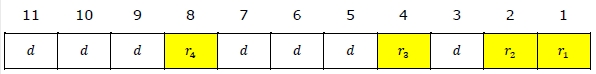
Step 3 − Calculating the values of each redundant bit.
The redundant bits are parity bits. A parity bit is an extra bit that makes the number of 1s either even or odd. The two types of parity are −
-
Even Parity − Here the total number of bits in the message is made even.
-
Odd Parity − Here the total number of bits in the message is made odd.
Each redundant bit, ri, is calculated as the parity, generally even parity, based upon its bit position. It covers all bit positions whose binary representation includes a 1 in the ith position except the position of ri. Thus −
-
r1 is the parity bit for all data bits in positions whose binary representation includes a 1 in the least significant position excluding 1 (3, 5, 7, 9, 11 and so on)
-
r2 is the parity bit for all data bits in positions whose binary representation includes a 1 in the position 2 from right except 2 (3, 6, 7, 10, 11 and so on)
-
r3 is the parity bit for all data bits in positions whose binary representation includes a 1 in the position 3 from right except 4 (5-7, 12-15, 20-23 and so on)
Example 3 − Suppose that the message 1100101 needs to be encoded using even parity Hamming code. Here, m = 7 and r comes to 4. The values of redundant bits will be as follows −
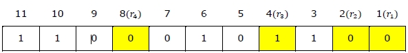
Hence, the message sent will be 11000101100.
Decoding a message in Hamming Code
Once the receiver gets an incoming message, it performs recalculations to detect errors and correct them. The steps for recalculation are −
-
Step 1 − Calculation of the number of redundant bits.
-
Step 2 − Positioning the redundant bits.
-
Step 3 − Parity checking.
-
Step 4 − Error detection and correction
Step 1) Calculation of the number of redundant bits
Using the same formula as in encoding, the number of redundant bits are ascertained.
2r ≥ 𝑚 + 𝑟 + 1
where m is the number of data bits and r is the number of redundant bits.
Step 2) Positioning the redundant bits
The r redundant bits placed at bit positions of powers of 2, i.e. 1, 2, 4, 8, 16 etc.
Step 3) Parity checking
Parity bits are calculated based upon the data bits and the redundant bits using the same rule as during generation of c1, c2, c3, c4 etc. Thus
c1 = parity(1, 3, 5, 7, 9, 11 and so on)
c2 = parity(2, 3, 6, 7, 10, 11 and so on)
c3 = parity(4-7, 12-15, 20-23 and so on)
Step 4) Error detection and correction
The decimal equivalent of the parity bits binary values is calculated. If it is 0, there is no error. Otherwise, the decimal value gives the bit position which has error. For example, if c1c2c3c4 = 1001, it implies that the data bit at position 9, decimal equivalent of 1001, has error. The bit is flipped (converted from 0 to 1 or vice versa) to get the correct message.
Example 4 − Suppose that an incoming message 11110101101 is received.
Step 1 − At first the number of redundant bits are calculated using the formula 2r ≥ m + r + 1. Here, m + r + 1 = 11 + 1 = 12. The minimum value of r such that 2r ≥ 12 is 4.
Step 2 − The redundant bits are positioned as below −
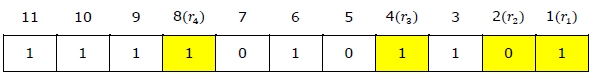
Step 3 − Even parity checking is done −
c1 = even_parity(1, 3, 5, 7, 9, 11) = 0
c2 = even_parity(2, 3, 6, 7, 10, 11) = 0
c3 = even_parity (4, 5, 6, 7) = 0
c4 = even_parity (8, 9, 10, 11) = 0
Step 4 — Since the value of the check bits c1c2c3c4 = 0000 = 0, there are no errors in this message.
Hamming Code for double error detection
The Hamming code can be modified to correct a single error and detect double errors by adding a parity bit as the MSB, which is the XOR of all other bits.
Example 5 − If we consider the codeword, 11000101100, sent as in example 3, after adding P = XOR(1,1,0,0,0,1,0,1,1,0,0) = 0, the new codeword to be sent will be 011000101100.
At the receiver’s end, error detection is done as shown in the following table −
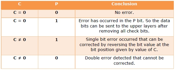
This is the approved revision of this page, as well as being the most recent.

Hamming code is a set of error-correction code s that can be used to detect and correct bit errors that can occur when computer data is moved or stored. The parity-check matrix of a Hamming code is constructed by listing all columns of length that are non-zero, which means that the [[duacode of the Hamming code is the shortened Hadamard code. The parity-check matrix has the property that any two columns are pairwise linearly independent.
Due to the limited redundancy that Hamming codes add to the data, they can only detect and correct errors when the error rate is low. This is the case in computer memory (ECC memory), where bit errors are extremely rare and Hamming codes are widely used. In this context, an extended Hamming code having one extra parity bit is often used. Extended Hamming codes achieve a Hamming distance of four, which allows the decoder to distinguish between when at most one one-bit error occurs and when any two-bit errors occur. In this sense, extended Hamming codes are single-error correcting and double-error detecting, abbreviated as SECDED.
Contents
-
1 Hamming and Hamming code theory
-
1.1 Codes predating Hamming
- 1.1.1 Parity
- 1.1.2 Two-out-of-five code
- 1.1.3 Repetition
-
1.1 Codes predating Hamming
-
2 Hamming codes
- 2.1 General algorithm – Hamming Code Error Correction
- 3 Hamming codes with additional parity (SECDED)
-
4 Hamming code 7-4
- 4.1 Construction of G and H
- 5 See also
- 6 Sources
Hamming and Hamming code theory[edit]
Richard Hamming, the inventor of Hamming codes, worked at Bell Labs in the 1940s on the Bell Model V computer, an electromechanical relay-based machine with cycle times in seconds. Input was fed in on punched paper tape, seven-eighths of an inch wide which had up to six holes per row. During weekdays, when errors in the relays were detected, the machine would stop and flash lights so that the operators could correct the problem. During after-hours periods and on weekends, when there were no operators, the machine simply moved on to the next job.
Hamming worked on weekends, and grew increasingly frustrated with having to restart his programs from scratch due to detected errors. In a taped interview Hamming said, «And so I said, ‘Damn it, if the machine can detect an error, why can’t it locate the position of the error and correct it?'». Over the next few years, he worked on the problem of error-correction, developing an increasingly powerful array of algorithms. In 1950, he published what is now known as Hamming Code, which remains in use today in applications such as ECC memory.
Codes predating Hamming[edit]
A number of simple error-detecting codes were used before Hamming codes, but none were as effective as Hamming codes in the same overhead of space.
Parity[edit]
Parity adds a single bit that indicates whether the number of ones (bit-positions with values of one) in the preceding data was even or odd. If an odd number of bits is changed in transmission, the message will change parity and the error can be detected at this point; however, the bit that changed may have been the parity bit itself. The most common convention is that a parity value of one indicates that there is an odd number of ones in the data, and a parity value of zero indicates that there is an even number of ones. If the number of bits changed is even, the check bit will be valid and the error will not be detected.
Moreover, parity does not indicate which bit contained the error, even when it can detect it. The data must be discarded entirely and re-transmitted from scratch. On a noisy transmission medium, a successful transmission could take a long time or may never occur. However, while the quality of parity checking is poor, since it uses only a single bit, this method results in the least overhead.
Two-out-of-five code[edit]
A two-out-of-five code is an encoding scheme which uses five bits consisting of exactly three 0s and two 1s. This provides ten possible combinations, enough to represent the digits 0–9. This scheme can detect all single bit-errors, all odd numbered bit-errors and some even numbered bit-errors (for example the flipping of both 1-bits). However it still cannot correct any of these errors.
Repetition[edit]
Another code in use at the time repeated every data bit multiple times in order to ensure that it was sent correctly. For instance, if the data bit to be sent is a 1, an repetition code will send 111. If the three bits received are not identical, an error occurred during transmission. If the channel is clean enough, most of the time only one bit will change in each triple. Therefore, 001, 010, and 100 each correspond to a 0 bit, while 110, 101, and 011 correspond to a 1 bit, with the greater quantity of digits that are the same (‘0’ or a ‘1’) indicating what the data bit should be. A code with this ability to reconstruct the original message in the presence of errors is known as an error-correcting code. This triple repetition code is a Hamming code with since there are two parity bits, and data bit.
Such codes cannot correctly repair all errors, however. In our example, if the channel flips two bits and the receiver gets 001, the system will detect the error, but conclude that the original bit is 0, which is incorrect. If we increase the size of the bit string to four, we can detect all two-bit errors but cannot correct them, (the quantity of parity bits is even) at five bits, we can correct all two-bit errors, but not all three-bit errors.
Moreover, increasing the size of the parity bit string is inefficient, reducing throughput by three times in our original case, and the efficiency drops drastically as we increase the number of times each bit is duplicated in order to detect and correct more errors.
Hamming codes[edit]
If more error-correcting bits are included with a message, and if those bits can be arranged such that different incorrect bits produce different error results, then bad bits could be identified. In a seven-bit message, there are seven possible single bit errors, so three error control bits could potentially specify not only that an error occurred but also which bit caused the error.
Hamming studied the existing coding schemes, including two-of-five, and generalized their concepts. To start with, he developed a nomenclature to describe the system, including the number of data bits and error-correction bits in a block. For instance, parity includes a single bit for any data word, so assuming ASCII words with seven bits, Hamming described this as an (8,7) code, with eight bits in total, of which seven are data. The repetition example would be (3,1), following the same logic. The code rate is the second number divided by the first, for our repetition example, 1/3.
Hamming also noticed the problems with flipping two or more bits, and described this as the «distance» (it is now called the Hamming distance, after him). Parity has a distance of 2, so one bit flip can be detected, but not corrected and any two bit flips will be invisible. The (3,1) repetition has a distance of 3, as three bits need to be flipped in the same triple to obtain another code word with no visible errors. It can correct one-bit errors or detect but not correct two-bit errors. A (4,1) repetition (each bit is repeated four times) has a distance of 4, so flipping three bits can be detected, but not corrected. When three bits flip in the same group there can be situations where attempting to correct will produce the wrong code word. In general, a code with distance k can detect but not correct errors.
Hamming was interested in two problems at once: increasing the distance as much as possible, while at the same time increasing the code rate as much as possible. During the 1940s he developed several encoding schemes that were dramatic improvements on existing codes. The key to all of his systems was to have the parity bits overlap, such that they managed to check each other as well as the data.
General algorithm – Hamming Code Error Correction[edit]
The following general algorithm generates a single-error correcting (SEC) code for any number of bits.
- Number the bits starting from 1: bit 1, 2, 3, 4, 5, etc.
- Write the bit numbers in binary: 1, 10, 11, 100, 101, etc.
- All bit positions that are powers of two (have a single 1 bit in the binary form of their position) are parity bits: 1, 2, 4, 8, etc. (1, 10, 100, 1000)
- All other bit positions, with two or more 1 bits in the binary form of their position, are data bits.
- Each data bit is included in a unique set of 2 or more parity bits, as determined by the binary form of its bit position.
- Parity bit 1 covers all bit positions which have the least significant bit set: bit 1 (the parity bit itself), 3, 5, 7, 9, etc.
- Parity bit 2 covers all bit positions which have the second least significant bit set: bit 2 (the parity bit itself), 3, 6, 7, 10, 11, etc.
- Parity bit 4 covers all bit positions which have the third least significant bit set: bits 4–7, 12–15, 20–23, etc.
- Parity bit 8 covers all bit positions which have the fourth least significant bit set: bits 8–15, 24–31, 40–47, etc.
- In general each parity bit covers all bits where the bitwise AND of the parity position and the bit position is non-zero.
The form of the parity is irrelevant. Even parity is mathematically simpler, but there is no difference in practice.
This general rule can be shown visually:

Shown are only 20 encoded bits (5 parity, 15 data) but the pattern continues indefinitely. The key thing about Hamming Codes that can be seen from visual inspection is that any given bit is included in a unique set of parity bits. To check for errors, check all of the parity bits. The pattern of errors, called the error syndrome, identifies the bit in error. If all parity bits are correct, there is no error. Otherwise, the sum of the positions of the erroneous parity bits identifies the erroneous bit. For example, if the parity bits in positions 1, 2 and 8 indicate an error, then bit 1+2+8=11 is in error. If only one parity bit indicates an error, the parity bit itself is in error.
As you can see, if you have parity bits, it can cover bits from 1 up to  . If we subtract out the parity bits, we are left with
  bits we can use for the data. As varies, we get all the possible Hamming codes:
| Parity bits | Total bits | Data bits | Name | Rate |
|---|---|---|---|---|
| 2 | 3 | 1 | Hamming(3,1) (Triple repetition code) |
1/3 ≈ 0.333 |
| 3 | 7 | 4 | Hamming(7,4) | 4/7 ≈ 0.571 |
| 4 | 15 | 11 | Hamming(15,11) | 11/15 ≈ 0.733 |
| 5 | 31 | 26 | Hamming(31,26) | 26/31 ≈ 0.839 |
| 6 | 63 | 57 | Hamming(63,57) | 57/63 ≈ 0.905 |
| 7 | 127 | 120 | Hamming(127,120) | 120/127 ≈ 0.945 |
| 8 | 255 | 247 | Hamming(255,247) | 247/255 ≈ 0.969 |
| … | ||||

|

|
Hamming
|

|
If, in addition, an overall parity bit (bit 0) is included, the code can detect (but not correct) any two-bit error, making a SECDED code. The overall parity indicates whether the total number of errors is even or odd. If the basic Hamming code detects an error, but the overall parity says that there are an even number of errors, an uncorrectable 2-bit error has occurred.
Hamming codes with additional parity (SECDED)[edit]
Hamming codes have a minimum distance of 3, which means that the decoder can detect and correct a single error, but it cannot distinguish a double bit error of some codeword from a single bit error of a different codeword. Thus, some double-bit errors will be incorrectly decoded as if they were single bit errors and therefore go undetected, unless no correction is attempted.
To remedy this shortcoming, Hamming codes can be extended by an extra parity bit. This way, it is possible to increase the minimum distance of the Hamming code to 4, which allows the decoder to distinguish between single bit errors and two-bit errors. Thus the decoder can detect and correct a single error and at the same time detect (but not correct) a double error. If the decoder does not attempt to correct errors, it can detect up to three errors.
This extended Hamming code is popular in computer memory systems, where it is known as SECDED (abbreviated from single error correction, double error detection). Particularly popular is the (72,64) code, a truncated (127,120) Hamming code plus an additional parity bit, which has the same space overhead as a (9,8) parity code.
Hamming code 7-4[edit]

Graphical depiction of the four data bits and three parity bits and which parity bits apply to which data bits
In 1950, Hamming introduced the Hamming code 7-4. It encodes four data bits into seven bits by adding three parity bits. It can detect and correct single-bit errors. With the addition of an overall parity bit, it can also detect (but not correct) double-bit errors.
Construction of G and H[edit]
The matrix
 is called a (canonical) generator matrix of a linear (n,k) code,
and  is called a parity-check matrix.
This is the construction of G and H in standard (or systematic) form. Regardless of form, G and H for linear block codes must satisfy
 , an all-zeros matrix.
Since [7, 4, 3] = [n, k, d] = [2m − 1, 2m−1−m, m]. The parity-check matrix H of a Hamming code is constructed by listing all columns of length m that are pair-wise independent.
Thus H is a matrix whose left side is all of the nonzero n-tuples where order of the n-tuples in the columns of matrix does not matter. The right hand side is just the (n − k)-identity matrix.
So G can be obtained from H by taking the transpose of the left hand side of H with the identity k-identity matrix on the left hand side of G.
The code generator matrix  and the parity-check matrix
  are:
are:

and

Finally, these matrices can be mutated into equivalent non-systematic codes by the following operations:.
The trick starts when a volunteer thinks of a number between 1 and 15 and a color, the magician shows colored cards with several numbers for the volunteer to say whether he sees his number, but he can lie on one card, according to the chosen color. The magician is able to find on which color the volunteer lied, and then tell the number.
Trick is based on the Hamming Code. The first four cards resemble a binary-digit trick with numbers 1 to 15. If there were no lie allowed, then we’d only need the first four cards. Simply, we would add the top left number on each card that faces up.
However, we are also trying to discover where the lie happened. This is similar to a computer system trying to fix a denigrated data communication. We need more digits (cards).
For every face-up card, you consider a 1 on the sequence. Face-down cards represent 0.
The first four cards will serve to compute the chosen number by adding the top-left number on cards facing up.
The last three cards are the «parity digits».
Check the parity digits (last three cards, see below), if only one of them does not match, then that is the «lie»-card, and the chosen number is the sum of the digits on top left on the first four cards that face up;
If more than one parity digit does not match, then you follow the rule, according to discrepancy:
— Parity 1 and 2: the person lied on the card 3 (yellow), so you flip the card, and the chosen number will be the sum of the numbers on top left on the first four cards who face up (after you «fixed» the sequence);
— Parity 1 and 3: the person lied on the card 2 (orange), so you flip the card, and the chosen number will be the sum of the numbers on top left on the first four cards who face up (after you «fixed» the sequence);
— Parity 2 and 3: the person lied on the card 1 (red), so you flip the card, and the chosen number will be the sum of the numbers on top left on the first four cards who face up (after you «fixed» the sequence);
— Parity 1, 2 and 3: the person lied on the card 4 (green), so you flip the card, and the chosen number will be the sum of the numbers on top left on the first four cards who face up (after you «fixed» the sequence).
You are creating a sequence of seven digits 0’s and 1’s. Because there is a lie, the final sequence will not be any one on the table on «Error Detection» section. With multiple parity checks, we are able to identify the incorrect digit, fix it, and find the correspondent number.
This magic trick appears on an article by Ricardo Teixeira on the February 2017 edition of Math Horizon («Decoding the Hamming Code,» Math Horizons, April 2006) and enhanced by Todd Mateer («A Magic Trick Based on the Hamming Code,» Math Horizons, November 2013). Ehrenborg’s and Mateer’s tricks, while essentially the same as this one, require specially designed cards with a clever but little complicated system of tabs to aid the magician. The advantage and disadvantage of using simple rectangular cards is that the trick happens in your mind, instead of physically on the cards.
See Also on BitcoinWiki[edit]
- Coding theory
- Reed–Muller code
- Reed–Solomon error correction
- Turbo code
- Low-density parity-check code
- Mining
Sources[edit]
http://wikipedia.org/
Improve Article
Save Article
Improve Article
Save Article
Hamming code is a set of error-correction codes that can be used to detect and correct the errors that can occur when the data is moved or stored from the sender to the receiver. It is a technique developed by R.W. Hamming for error correction. Redundant bits – Redundant bits are extra binary bits that are generated and added to the information-carrying bits of data transfer to ensure that no bits were lost during the data transfer. The number of redundant bits can be calculated using the following formula:
 2^r ≥ m + r + 1
 where, r = redundant bit, m = data bit
Suppose the number of data bits is 7, then the number of redundant bits can be calculated using: = 2^4 ≥ 7 + 4 + 1 Thus, the number of redundant bits= 4 Parity bits. A parity bit is a bit appended to a data of binary bits to ensure that the total number of 1’s in the data is even or odd. Parity bits are used for error detection. There are two types of parity bits:
- Even parity bit: In the case of even parity, for a given set of bits, the number of 1’s are counted. If that count is odd, the parity bit value is set to 1, making the total count of occurrences of 1’s an even number. If the total number of 1’s in a given set of bits is already even, the parity bit’s value is 0.
- Odd Parity bit – In the case of odd parity, for a given set of bits, the number of 1’s are counted. If that count is even, the parity bit value is set to 1, making the total count of occurrences of 1’s an odd number. If the total number of 1’s in a given set of bits is already odd, the parity bit’s value is 0.
General Algorithm of Hamming code: Hamming Code is simply the use of extra parity bits to allow the identification of an error.
- Write the bit positions starting from 1 in binary form (1, 10, 11, 100, etc).
- All the bit positions that are a power of 2 are marked as parity bits (1, 2, 4, 8, etc).
- All the other bit positions are marked as data bits.
- Each data bit is included in a unique set of parity bits, as determined its bit position in binary form. a. Parity bit 1 covers all the bits positions whose binary representation includes a 1 in the least significant position (1, 3, 5, 7, 9, 11, etc). b. Parity bit 2 covers all the bits positions whose binary representation includes a 1 in the second position from the least significant bit (2, 3, 6, 7, 10, 11, etc). c. Parity bit 4 covers all the bits positions whose binary representation includes a 1 in the third position from the least significant bit (4–7, 12–15, 20–23, etc). d. Parity bit 8 covers all the bits positions whose binary representation includes a 1 in the fourth position from the least significant bit bits (8–15, 24–31, 40–47, etc). e. In general, each parity bit covers all bits where the bitwise AND of the parity position and the bit position is non-zero.
- Since we check for even parity set a parity bit to 1 if the total number of ones in the positions it checks is odd.
- Set a parity bit to 0 if the total number of ones in the positions it checks is even.
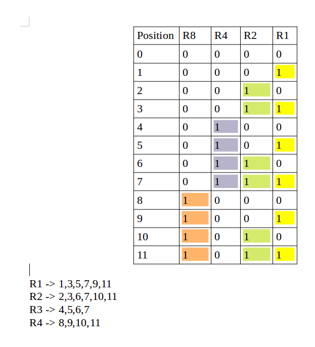
Determining the position of redundant bits – These redundancy bits are placed at positions that correspond to the power of 2.
As in the above example:
- The number of data bits = 7
- The number of redundant bits = 4
- The total number of bits = 11
- The redundant bits are placed at positions corresponding to power of 2- 1, 2, 4, and 8
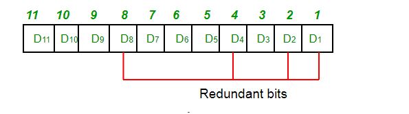
- Suppose the data to be transmitted is 1011001, the bits will be placed as follows:
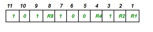
Determining the Parity bits:
- R1 bit is calculated using parity check at all the bits positions whose binary representation includes a 1 in the least significant position. R1: bits 1, 3, 5, 7, 9, 11
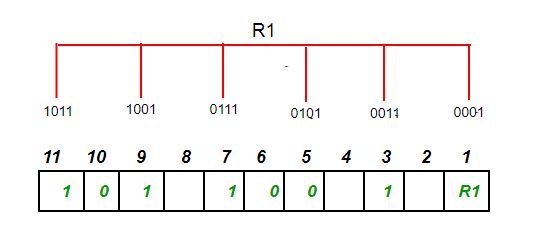
- To find the redundant bit R1, we check for even parity. Since the total number of 1’s in all the bit positions corresponding to R1 is an even number the value of R1 (parity bit’s value) = 0
- R2 bit is calculated using parity check at all the bits positions whose binary representation includes a 1 in the second position from the least significant bit. R2: bits 2,3,6,7,10,11
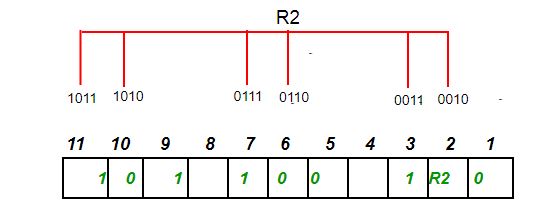
- To find the redundant bit R2, we check for even parity. Since the total number of 1’s in all the bit positions corresponding to R2 is odd the value of R2(parity bit’s value)=1
- R4 bit is calculated using parity check at all the bits positions whose binary representation includes a 1 in the third position from the least significant bit. R4: bits 4, 5, 6, 7
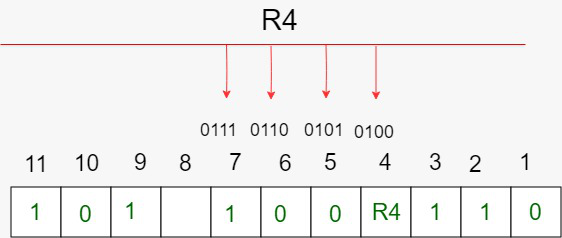
- To find the redundant bit R4, we check for even parity. Since the total number of 1’s in all the bit positions corresponding to R4 is odd the value of R4(parity bit’s value) = 1
- R8 bit is calculated using parity check at all the bits positions whose binary representation includes a 1 in the fourth position from the least significant bit. R8: bit 8,9,10,11

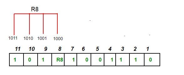
- To find the redundant bit R8, we check for even parity. Since the total number of 1’s in all the bit positions corresponding to R8 is an even number the value of R8(parity bit’s value)=0. Thus, the data transferred is:
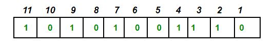
Error detection and correction: Suppose in the above example the 6th bit is changed from 0 to 1 during data transmission, then it gives new parity values in the binary number:
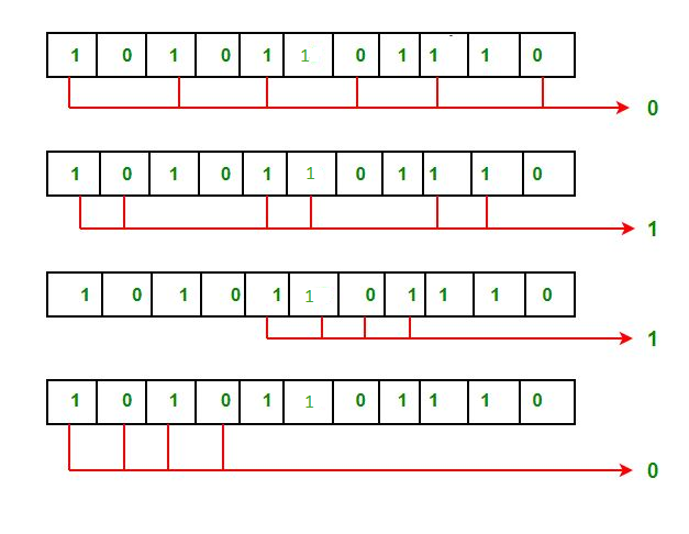
The bits give the binary number 0110 whose decimal representation is 6. Thus, bit 6 contains an error. To correct the error the 6th bit is changed from 1 to 0.