Imaginary error function

Error function
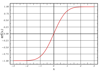
Plot of the error function
General information
General definition	${displaystyle operatorname {erf} z={frac {2}{sqrt {pi }}}int _{0}^{z}e^{-t^{2}},mathrm {d} t}$
Fields of application	Probability, thermodynamics
Domain, Codomain and Image
Domain
Image
Basic features
Parity	Odd
Specific features
Root	0
Derivative	${displaystyle {frac {mathrm {d} }{mathrm {d} z}}operatorname {erf} z={frac {2}{sqrt {pi }}}e^{-z^{2}}}$
Antiderivative	${displaystyle int operatorname {erf} z,dz=zoperatorname {erf} z+{frac {e^{-z^{2}}}{sqrt {pi }}}+C}$
Series definition
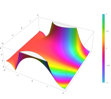
Taylor series	${displaystyle operatorname {erf} z={frac {2}{sqrt {pi }}}sum _{n=0}^{infty }{frac {z}{2n+1}}prod _{k=1}^{n}{frac {-z^{2}}{k}}}$

In mathematics, the error function (also called the Gauss error function), often denoted by erf, is a complex function of a complex variable defined as:^[1]

${displaystyle operatorname {erf} z={frac {2}{sqrt {pi }}}int _{0}^{z}e^{-t^{2}},mathrm {d} t.}$

This integral is a special (non-elementary) sigmoid function that occurs often in probability, statistics, and partial differential equations. In many of these applications, the function argument is a real number. If the function argument is real, then the function value is also real.

In statistics, for non-negative values of x, the error function has the following interpretation: for a random variable Y that is normally distributed with mean 0 and standard deviation 1/√2, erf x is the probability that Y falls in the range [−x, x].

Two closely related functions are the complementary error function (erfc) defined as

{displaystyle operatorname {erfc} z=1-operatorname {erf} z,}

and the imaginary error function (erfi) defined as

{displaystyle operatorname {erfi} z=-ioperatorname {erf} iz,}

where i is the imaginary unit

Name[edit]

The name «error function» and its abbreviation erf were proposed by J. W. L. Glaisher in 1871 on account of its connection with «the theory of Probability, and notably the theory of Errors.»^[2] The error function complement was also discussed by Glaisher in a separate publication in the same year.^[3]
For the «law of facility» of errors whose density is given by

${displaystyle f(x)=left({frac {c}{pi }}right)^{frac {1}{2}}e^{-cx^{2}}}$

(the normal distribution), Glaisher calculates the probability of an error lying between p and q as:

${displaystyle left({frac {c}{pi }}right)^{frac {1}{2}}int _{p}^{q}e^{-cx^{2}},mathrm {d} x={tfrac {1}{2}}left(operatorname {erf} left(q{sqrt {c}}right)-operatorname {erf} left(p{sqrt {c}}right)right).}$

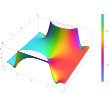
Plot of the error function Erf(z) in the complex plane from -2-2i to 2+2i with colors created with Mathematica 13.1 function ComplexPlot3D

Applications[edit]

When the results of a series of measurements are described by a normal distribution with standard deviation σ and expected value 0, then erf (a/σ √2) is the probability that the error of a single measurement lies between −a and +a, for positive a. This is useful, for example, in determining the bit error rate of a digital communication system.

The error and complementary error functions occur, for example, in solutions of the heat equation when boundary conditions are given by the Heaviside step function.

The error function and its approximations can be used to estimate results that hold with high probability or with low probability. Given a random variable X ~ Norm[μ,σ] (a normal distribution with mean μ and standard deviation σ) and a constant L < μ:

${displaystyle {begin{aligned}Pr[Xleq L]&={frac {1}{2}}+{frac {1}{2}}operatorname {erf} {frac {L-mu }{{sqrt {2}}sigma }}\&approx Aexp left(-Bleft({frac {L-mu }{sigma }}right)^{2}right)end{aligned}}}$

where A and B are certain numeric constants. If L is sufficiently far from the mean, specifically μ − L ≥ σ√ln k, then:

${displaystyle Pr[Xleq L]leq Aexp(-Bln {k})={frac {A}{k^{B}}}}$

so the probability goes to 0 as k → ∞.

The probability for X being in the interval [L_a, L_b] can be derived as

${displaystyle {begin{aligned}Pr[L_{a}leq Xleq L_{b}]&=int _{L_{a}}^{L_{b}}{frac {1}{{sqrt {2pi }}sigma }}exp left(-{frac {(x-mu )^{2}}{2sigma ^{2}}}right),mathrm {d} x\&={frac {1}{2}}left(operatorname {erf} {frac {L_{b}-mu }{{sqrt {2}}sigma }}-operatorname {erf} {frac {L_{a}-mu }{{sqrt {2}}sigma }}right).end{aligned}}}$

Properties[edit]

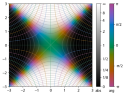
Integrand exp(−z²)

erf z

The property erf (−z) = −erf z means that the error function is an odd function. This directly results from the fact that the integrand e^−t² is an even function (the antiderivative of an even function which is zero at the origin is an odd function and vice versa).

Since the error function is an entire function which takes real numbers to real numbers, for any complex number z:

{displaystyle operatorname {erf} {overline {z}}={overline {operatorname {erf} z}}}

where z is the complex conjugate of z.

The integrand f = exp(−z²) and f = erf z are shown in the complex z-plane in the figures at right with domain coloring.

The error function at +∞ is exactly 1 (see Gaussian integral). At the real axis, erf z approaches unity at z → +∞ and −1 at z → −∞. At the imaginary axis, it tends to ±i∞.

Taylor series[edit]

The error function is an entire function; it has no singularities (except that at infinity) and its Taylor expansion always converges, but is famously known «[…] for its bad convergence if x > 1.»^[4]

The defining integral cannot be evaluated in closed form in terms of elementary functions, but by expanding the integrand e^−z² into its Maclaurin series and integrating term by term, one obtains the error function’s Maclaurin series as:

${displaystyle {begin{aligned}operatorname {erf} z&={frac {2}{sqrt {pi }}}sum _{n=0}^{infty }{frac {(-1)^{n}z^{2n+1}}{n!(2n+1)}}\[6pt]&={frac {2}{sqrt {pi }}}left(z-{frac {z^{3}}{3}}+{frac {z^{5}}{10}}-{frac {z^{7}}{42}}+{frac {z^{9}}{216}}-cdots right)end{aligned}}}$

which holds for every complex number z. The denominator terms are sequence A007680 in the OEIS.

For iterative calculation of the above series, the following alternative formulation may be useful:

${displaystyle {begin{aligned}operatorname {erf} z&={frac {2}{sqrt {pi }}}sum _{n=0}^{infty }left(zprod _{k=1}^{n}{frac {-(2k-1)z^{2}}{k(2k+1)}}right)\[6pt]&={frac {2}{sqrt {pi }}}sum _{n=0}^{infty }{frac {z}{2n+1}}prod _{k=1}^{n}{frac {-z^{2}}{k}}end{aligned}}}$

because −(2k − 1)z²/k(2k + 1) expresses the multiplier to turn the kth term into the (k + 1)th term (considering z as the first term).

The imaginary error function has a very similar Maclaurin series, which is:

${displaystyle {begin{aligned}operatorname {erfi} z&={frac {2}{sqrt {pi }}}sum _{n=0}^{infty }{frac {z^{2n+1}}{n!(2n+1)}}\[6pt]&={frac {2}{sqrt {pi }}}left(z+{frac {z^{3}}{3}}+{frac {z^{5}}{10}}+{frac {z^{7}}{42}}+{frac {z^{9}}{216}}+cdots right)end{aligned}}}$

which holds for every complex number z.

Derivative and integral[edit]

The derivative of the error function follows immediately from its definition:

${displaystyle {frac {mathrm {d} }{mathrm {d} z}}operatorname {erf} z={frac {2}{sqrt {pi }}}e^{-z^{2}}.}$

From this, the derivative of the imaginary error function is also immediate:

${displaystyle {frac {d}{dz}}operatorname {erfi} z={frac {2}{sqrt {pi }}}e^{z^{2}}.}$

An antiderivative of the error function, obtainable by integration by parts, is

${displaystyle zoperatorname {erf} z+{frac {e^{-z^{2}}}{sqrt {pi }}}.}$

An antiderivative of the imaginary error function, also obtainable by integration by parts, is

${displaystyle zoperatorname {erfi} z-{frac {e^{z^{2}}}{sqrt {pi }}}.}$

Higher order derivatives are given by

${displaystyle operatorname {erf} ^{(k)}z={frac {2(-1)^{k-1}}{sqrt {pi }}}{mathit {H}}_{k-1}(z)e^{-z^{2}}={frac {2}{sqrt {pi }}}{frac {mathrm {d} ^{k-1}}{mathrm {d} z^{k-1}}}left(e^{-z^{2}}right),qquad k=1,2,dots }$

where H are the physicists’ Hermite polynomials.^[5]

Bürmann series[edit]

An expansion,^[6] which converges more rapidly for all real values of x than a Taylor expansion, is obtained by using Hans Heinrich Bürmann’s theorem:^[7]

${displaystyle {begin{aligned}operatorname {erf} x&={frac {2}{sqrt {pi }}}operatorname {sgn} xcdot {sqrt {1-e^{-x^{2}}}}left(1-{frac {1}{12}}left(1-e^{-x^{2}}right)-{frac {7}{480}}left(1-e^{-x^{2}}right)^{2}-{frac {5}{896}}left(1-e^{-x^{2}}right)^{3}-{frac {787}{276480}}left(1-e^{-x^{2}}right)^{4}-cdots right)\[10pt]&={frac {2}{sqrt {pi }}}operatorname {sgn} xcdot {sqrt {1-e^{-x^{2}}}}left({frac {sqrt {pi }}{2}}+sum _{k=1}^{infty }c_{k}e^{-kx^{2}}right).end{aligned}}}$

where sgn is the sign function. By keeping only the first two coefficients and choosing c₁ = 31/200 and c₂ = −341/8000, the resulting approximation shows its largest relative error at x = ±1.3796, where it is less than 0.0036127:

${displaystyle operatorname {erf} xapprox {frac {2}{sqrt {pi }}}operatorname {sgn} xcdot {sqrt {1-e^{-x^{2}}}}left({frac {sqrt {pi }}{2}}+{frac {31}{200}}e^{-x^{2}}-{frac {341}{8000}}e^{-2x^{2}}right).}$

Inverse functions[edit]

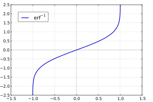
Given a complex number z, there is not a unique complex number w satisfying erf w = z, so a true inverse function would be multivalued. However, for −1 < x < 1, there is a unique real number denoted erf⁻¹ x satisfying

${displaystyle operatorname {erf} left(operatorname {erf} ^{-1}xright)=x.}$

The inverse error function is usually defined with domain (−1,1), and it is restricted to this domain in many computer algebra systems. However, it can be extended to the disk |z| < 1 of the complex plane, using the Maclaurin series

${displaystyle operatorname {erf} ^{-1}z=sum _{k=0}^{infty }{frac {c_{k}}{2k+1}}left({frac {sqrt {pi }}{2}}zright)^{2k+1},}$

where c₀ = 1 and

${displaystyle {begin{aligned}c_{k}&=sum _{m=0}^{k-1}{frac {c_{m}c_{k-1-m}}{(m+1)(2m+1)}}\&=left{1,1,{frac {7}{6}},{frac {127}{90}},{frac {4369}{2520}},{frac {34807}{16200}},ldots right}.end{aligned}}}$

So we have the series expansion (common factors have been canceled from numerators and denominators):

${displaystyle operatorname {erf} ^{-1}z={frac {sqrt {pi }}{2}}left(z+{frac {pi }{12}}z^{3}+{frac {7pi ^{2}}{480}}z^{5}+{frac {127pi ^{3}}{40320}}z^{7}+{frac {4369pi ^{4}}{5806080}}z^{9}+{frac {34807pi ^{5}}{182476800}}z^{11}+cdots right).}$

(After cancellation the numerator/denominator fractions are entries OEIS: A092676/OEIS: A092677 in the OEIS; without cancellation the numerator terms are given in entry OEIS: A002067.) The error function’s value at ±∞ is equal to ±1.

For |z| < 1, we have erf(erf⁻¹ z) = z.

The inverse complementary error function is defined as

${displaystyle operatorname {erfc} ^{-1}(1-z)=operatorname {erf} ^{-1}z.}$

For real x, there is a unique real number erfi⁻¹ x satisfying erfi(erfi⁻¹ x) = x. The inverse imaginary error function is defined as erfi⁻¹ x.^[8]

For any real x, Newton’s method can be used to compute erfi⁻¹ x, and for −1 ≤ x ≤ 1, the following Maclaurin series converges:

${displaystyle operatorname {erfi} ^{-1}z=sum _{k=0}^{infty }{frac {(-1)^{k}c_{k}}{2k+1}}left({frac {sqrt {pi }}{2}}zright)^{2k+1},}$

where c_k is defined as above.

Asymptotic expansion[edit]

A useful asymptotic expansion of the complementary error function (and therefore also of the error function) for large real x is

${displaystyle {begin{aligned}operatorname {erfc} x&={frac {e^{-x^{2}}}{x{sqrt {pi }}}}left(1+sum _{n=1}^{infty }(-1)^{n}{frac {1cdot 3cdot 5cdots (2n-1)}{left(2x^{2}right)^{n}}}right)\[6pt]&={frac {e^{-x^{2}}}{x{sqrt {pi }}}}sum _{n=0}^{infty }(-1)^{n}{frac {(2n-1)!!}{left(2x^{2}right)^{n}}},end{aligned}}}$

where (2n − 1)!! is the double factorial of (2n − 1), which is the product of all odd numbers up to (2n − 1). This series diverges for every finite x, and its meaning as asymptotic expansion is that for any integer N ≥ 1 one has

${displaystyle operatorname {erfc} x={frac {e^{-x^{2}}}{x{sqrt {pi }}}}sum _{n=0}^{N-1}(-1)^{n}{frac {(2n-1)!!}{left(2x^{2}right)^{n}}}+R_{N}(x)}$

where the remainder, in Landau notation, is

${displaystyle R_{N}(x)=Oleft(x^{-(1+2N)}e^{-x^{2}}right)}$

as x → ∞.

Indeed, the exact value of the remainder is

${displaystyle R_{N}(x):={frac {(-1)^{N}}{sqrt {pi }}}2^{1-2N}{frac {(2N)!}{N!}}int _{x}^{infty }t^{-2N}e^{-t^{2}},mathrm {d} t,}$

which follows easily by induction, writing

${displaystyle e^{-t^{2}}=-(2t)^{-1}left(e^{-t^{2}}right)'}$

and integrating by parts.

For large enough values of x, only the first few terms of this asymptotic expansion are needed to obtain a good approximation of erfc x (while for not too large values of x, the above Taylor expansion at 0 provides a very fast convergence).

Continued fraction expansion[edit]

A continued fraction expansion of the complementary error function is:^[9]

${displaystyle operatorname {erfc} z={frac {z}{sqrt {pi }}}e^{-z^{2}}{cfrac {1}{z^{2}+{cfrac {a_{1}}{1+{cfrac {a_{2}}{z^{2}+{cfrac {a_{3}}{1+dotsb }}}}}}}},qquad a_{m}={frac {m}{2}}.}$

Integral of error function with Gaussian density function[edit]

${displaystyle int _{-infty }^{infty }operatorname {erf} left(ax+bright){frac {1}{sqrt {2pi sigma ^{2}}}}exp left(-{frac {(x-mu )^{2}}{2sigma ^{2}}}right),mathrm {d} x=operatorname {erf} {frac {amu +b}{sqrt {1+2a^{2}sigma ^{2}}}},qquad a,b,mu ,sigma in mathbb {R} }$

which appears related to Ng and Geller, formula 13 in section 4.3^[10] with a change of variables.

Factorial series[edit]

The inverse factorial series:

${displaystyle {begin{aligned}operatorname {erfc} z&={frac {e^{-z^{2}}}{{sqrt {pi }},z}}sum _{n=0}^{infty }{frac {(-1)^{n}Q_{n}}{{(z^{2}+1)}^{bar {n}}}}\&={frac {e^{-z^{2}}}{{sqrt {pi }},z}}left(1-{frac {1}{2}}{frac {1}{(z^{2}+1)}}+{frac {1}{4}}{frac {1}{(z^{2}+1)(z^{2}+2)}}-cdots right)end{aligned}}}$

converges for Re(z²) > 0. Here

${displaystyle {begin{aligned}Q_{n}&{overset {text{def}}{{}={}}}{frac {1}{Gamma left({frac {1}{2}}right)}}int _{0}^{infty }tau (tau -1)cdots (tau -n+1)tau ^{-{frac {1}{2}}}e^{-tau },dtau \&=sum _{k=0}^{n}left({tfrac {1}{2}}right)^{bar {k}}s(n,k),end{aligned}}}$

zⁿ denotes the rising factorial, and s(n,k) denotes a signed Stirling number of the first kind.^[11]^[12]
There also exists a representation by an infinite sum containing the double factorial:

${displaystyle operatorname {erf} z={frac {2}{sqrt {pi }}}sum _{n=0}^{infty }{frac {(-2)^{n}(2n-1)!!}{(2n+1)!}}z^{2n+1}}$

Numerical approximations[edit]

Approximation with elementary functions[edit]

Abramowitz and Stegun give several approximations of varying accuracy (equations 7.1.25–28). This allows one to choose the fastest approximation suitable for a given application. In order of increasing accuracy, they are:

${displaystyle operatorname {erf} xapprox 1-{frac {1}{left(1+a_{1}x+a_{2}x^{2}+a_{3}x^{3}+a_{4}x^{4}right)^{4}}},qquad xgeq 0}$

(maximum error: 5×10⁻⁴)

where a₁ = 0.278393, a₂ = 0.230389, a₃ = 0.000972, a₄ = 0.078108

${displaystyle operatorname {erf} xapprox 1-left(a_{1}t+a_{2}t^{2}+a_{3}t^{3}right)e^{-x^{2}},quad t={frac {1}{1+px}},qquad xgeq 0}$

(maximum error: 2.5×10⁻⁵)

where p = 0.47047, a₁ = 0.3480242, a₂ = −0.0958798, a₃ = 0.7478556

${displaystyle operatorname {erf} xapprox 1-{frac {1}{left(1+a_{1}x+a_{2}x^{2}+cdots +a_{6}x^{6}right)^{16}}},qquad xgeq 0}$

(maximum error: 3×10⁻⁷)

where a₁ = 0.0705230784, a₂ = 0.0422820123, a₃ = 0.0092705272, a₄ = 0.0001520143, a₅ = 0.0002765672, a₆ = 0.0000430638

${displaystyle operatorname {erf} xapprox 1-left(a_{1}t+a_{2}t^{2}+cdots +a_{5}t^{5}right)e^{-x^{2}},quad t={frac {1}{1+px}}}$

(maximum error: 1.5×10⁻⁷)

where p = 0.3275911, a₁ = 0.254829592, a₂ = −0.284496736, a₃ = 1.421413741, a₄ = −1.453152027, a₅ = 1.061405429

All of these approximations are valid for x ≥ 0. To use these approximations for negative x, use the fact that erf x is an odd function, so erf x = −erf(−x).
Exponential bounds and a pure exponential approximation for the complementary error function are given by^[13]

${displaystyle {begin{aligned}operatorname {erfc} x&leq {tfrac {1}{2}}e^{-2x^{2}}+{tfrac {1}{2}}e^{-x^{2}}leq e^{-x^{2}},&quad x&>0\operatorname {erfc} x&approx {tfrac {1}{6}}e^{-x^{2}}+{tfrac {1}{2}}e^{-{frac {4}{3}}x^{2}},&quad x&>0.end{aligned}}}$
The above have been generalized to sums of N exponentials^[14] with increasing accuracy in terms of N so that erfc x can be accurately approximated or bounded by 2Q̃(√2x), where

${displaystyle {tilde {Q}}(x)=sum _{n=1}^{N}a_{n}e^{-b_{n}x^{2}}.}$

In particular, there is a systematic methodology to solve the numerical coefficients {(a_n,b_n)}^N
_{n = 1} that yield a minimax approximation or bound for the closely related Q-function: Q(x) ≈ Q̃(x), Q(x) ≤ Q̃(x), or Q(x) ≥ Q̃(x) for x ≥ 0. The coefficients {(a_n,b_n)}^N
_{n = 1} for many variations of the exponential approximations and bounds up to N = 25 have been released to open access as a comprehensive dataset.^[15]
A tight approximation of the complementary error function for x ∈ [0,∞) is given by Karagiannidis & Lioumpas (2007)^[16] who showed for the appropriate choice of parameters {A,B} that

${displaystyle operatorname {erfc} xapprox {frac {left(1-e^{-Ax}right)e^{-x^{2}}}{B{sqrt {pi }}x}}.}$

They determined {A,B} = {1.98,1.135}, which gave a good approximation for all x ≥ 0. Alternative coefficients are also available for tailoring accuracy for a specific application or transforming the expression into a tight bound.^[17]
A single-term lower bound is^[18]

${displaystyle operatorname {erfc} xgeq {sqrt {frac {2e}{pi }}}{frac {sqrt {beta -1}}{beta }}e^{-beta x^{2}},qquad xgeq 0,quad beta >1,}$

where the parameter β can be picked to minimize error on the desired interval of approximation.
Another approximation is given by Sergei Winitzki using his «global Padé approximations»:^[19]^[20]^: 2–3

${displaystyle operatorname {erf} xapprox operatorname {sgn} xcdot {sqrt {1-exp left(-x^{2}{frac {{frac {4}{pi }}+ax^{2}}{1+ax^{2}}}right)}}}$

where

${displaystyle a={frac {8(pi -3)}{3pi (4-pi )}}approx 0.140012.}$

This is designed to be very accurate in a neighborhood of 0 and a neighborhood of infinity, and the relative error is less than 0.00035 for all real x. Using the alternate value a ≈ 0.147 reduces the maximum relative error to about 0.00013.^[21]

This approximation can be inverted to obtain an approximation for the inverse error function:

${displaystyle operatorname {erf} ^{-1}xapprox operatorname {sgn} xcdot {sqrt {{sqrt {left({frac {2}{pi a}}+{frac {ln left(1-x^{2}right)}{2}}right)^{2}-{frac {ln left(1-x^{2}right)}{a}}}}-left({frac {2}{pi a}}+{frac {ln left(1-x^{2}right)}{2}}right)}}.}$
An approximation with a maximal error of 1.2×10⁻⁷ for any real argument is:^[22]

${displaystyle operatorname {erf} x={begin{cases}1-tau &xgeq 0\tau -1&x<0end{cases}}}$

with

${displaystyle {begin{aligned}tau &=tcdot exp left(-x^{2}-1.26551223+1.00002368t+0.37409196t^{2}+0.09678418t^{3}-0.18628806t^{4}right.\&left.qquad qquad qquad +0.27886807t^{5}-1.13520398t^{6}+1.48851587t^{7}-0.82215223t^{8}+0.17087277t^{9}right)end{aligned}}}$

and

${displaystyle t={frac {1}{1+{frac {1}{2}}|x|}}.}$

Table of values[edit]

x	erf x	1 − erf x
0	0	1
0.02	0.022564575	0.977435425
0.04	0.045111106	0.954888894
0.06	0.067621594	0.932378406
0.08	0.090078126	0.909921874
0.1	0.112462916	0.887537084
0.2	0.222702589	0.777297411
0.3	0.328626759	0.671373241
0.4	0.428392355	0.571607645
0.5	0.520499878	0.479500122
0.6	0.603856091	0.396143909
0.7	0.677801194	0.322198806
0.8	0.742100965	0.257899035
0.9	0.796908212	0.203091788
1	0.842700793	0.157299207
1.1	0.880205070	0.119794930
1.2	0.910313978	0.089686022
1.3	0.934007945	0.065992055
1.4	0.952285120	0.047714880
1.5	0.966105146	0.033894854
1.6	0.976348383	0.023651617
1.7	0.983790459	0.016209541
1.8	0.989090502	0.010909498
1.9	0.992790429	0.007209571
2	0.995322265	0.004677735
2.1	0.997020533	0.002979467
2.2	0.998137154	0.001862846
2.3	0.998856823	0.001143177
2.4	0.999311486	0.000688514
2.5	0.999593048	0.000406952
3	0.999977910	0.000022090
3.5	0.999999257	0.000000743

[edit]

Complementary error function[edit]

The complementary error function, denoted erfc, is defined as

Plot of the complementary error function Erfc(z) in the complex plane from -2-2i to 2+2i with colors created with Mathematica 13.1 function ComplexPlot3D

${displaystyle {begin{aligned}operatorname {erfc} x&=1-operatorname {erf} x\[5pt]&={frac {2}{sqrt {pi }}}int _{x}^{infty }e^{-t^{2}},mathrm {d} t\[5pt]&=e^{-x^{2}}operatorname {erfcx} x,end{aligned}}}$

which also defines erfcx, the scaled complementary error function^[23] (which can be used instead of erfc to avoid arithmetic underflow^[23]^[24]). Another form of erfc x for x ≥ 0 is known as Craig’s formula, after its discoverer:^[25]

${displaystyle operatorname {erfc} (xmid xgeq 0)={frac {2}{pi }}int _{0}^{frac {pi }{2}}exp left(-{frac {x^{2}}{sin ^{2}theta }}right),mathrm {d} theta .}$

This expression is valid only for positive values of x, but it can be used in conjunction with erfc x = 2 − erfc(−x) to obtain erfc(x) for negative values. This form is advantageous in that the range of integration is fixed and finite. An extension of this expression for the erfc of the sum of two non-negative variables is as follows:^[26]

${displaystyle operatorname {erfc} (x+ymid x,ygeq 0)={frac {2}{pi }}int _{0}^{frac {pi }{2}}exp left(-{frac {x^{2}}{sin ^{2}theta }}-{frac {y^{2}}{cos ^{2}theta }}right),mathrm {d} theta .}$

Imaginary error function[edit]

The imaginary error function, denoted erfi, is defined as

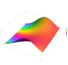
Plot of the imaginary error function Erfi(z) in the complex plane from -2-2i to 2+2i with colors created with Mathematica 13.1 function ComplexPlot3D

${displaystyle {begin{aligned}operatorname {erfi} x&=-ioperatorname {erf} ix\[5pt]&={frac {2}{sqrt {pi }}}int _{0}^{x}e^{t^{2}},mathrm {d} t\[5pt]&={frac {2}{sqrt {pi }}}e^{x^{2}}D(x),end{aligned}}}$

where D(x) is the Dawson function (which can be used instead of erfi to avoid arithmetic overflow^[23]).

Despite the name «imaginary error function», erfi x is real when x is real.

When the error function is evaluated for arbitrary complex arguments z, the resulting complex error function is usually discussed in scaled form as the Faddeeva function:

$w(z)=e^{-z^{2}}operatorname {erfc} (-iz)=operatorname {erfcx} (-iz).$

Cumulative distribution function[edit]

The error function is essentially identical to the standard normal cumulative distribution function, denoted Φ, also named norm(x) by some software languages^{[citation needed]}, as they differ only by scaling and translation. Indeed,

the normal cumulative distribution function plotted in the complex plane

${displaystyle {begin{aligned}Phi (x)&={frac {1}{sqrt {2pi }}}int _{-infty }^{x}e^{tfrac {-t^{2}}{2}},mathrm {d} t\[6pt]&={frac {1}{2}}left(1+operatorname {erf} {frac {x}{sqrt {2}}}right)\[6pt]&={frac {1}{2}}operatorname {erfc} left(-{frac {x}{sqrt {2}}}right)end{aligned}}}$

or rearranged for erf and erfc:

${displaystyle {begin{aligned}operatorname {erf} (x)&=2Phi left(x{sqrt {2}}right)-1\[6pt]operatorname {erfc} (x)&=2Phi left(-x{sqrt {2}}right)\&=2left(1-Phi left(x{sqrt {2}}right)right).end{aligned}}}$

Consequently, the error function is also closely related to the Q-function, which is the tail probability of the standard normal distribution. The Q-function can be expressed in terms of the error function as

${displaystyle {begin{aligned}Q(x)&={frac {1}{2}}-{frac {1}{2}}operatorname {erf} {frac {x}{sqrt {2}}}\&={frac {1}{2}}operatorname {erfc} {frac {x}{sqrt {2}}}.end{aligned}}}$

The inverse of Φ is known as the normal quantile function, or probit function and may be expressed in terms of the inverse error function as

${displaystyle operatorname {probit} (p)=Phi ^{-1}(p)={sqrt {2}}operatorname {erf} ^{-1}(2p-1)=-{sqrt {2}}operatorname {erfc} ^{-1}(2p).}$

The standard normal cdf is used more often in probability and statistics, and the error function is used more often in other branches of mathematics.

The error function is a special case of the Mittag-Leffler function, and can also be expressed as a confluent hypergeometric function (Kummer’s function):

${displaystyle operatorname {erf} x={frac {2x}{sqrt {pi }}}Mleft({tfrac {1}{2}},{tfrac {3}{2}},-x^{2}right).}$

It has a simple expression in terms of the Fresnel integral.^{[further explanation needed]}

In terms of the regularized gamma function P and the incomplete gamma function,

${displaystyle operatorname {erf} x=operatorname {sgn} xcdot Pleft({tfrac {1}{2}},x^{2}right)={frac {operatorname {sgn} x}{sqrt {pi }}}gamma left({tfrac {1}{2}},x^{2}right).}$

sgn x is the sign function.

Generalized error functions[edit]

Graph of generalised error functions E_n(x):
grey curve: E₁(x) = 1 − e^−x/√π
red curve: E₂(x) = erf(x)
green curve: E₃(x)
blue curve: E₄(x)
gold curve: E₅(x).

Some authors discuss the more general functions:^{[citation needed]}

${displaystyle E_{n}(x)={frac {n!}{sqrt {pi }}}int _{0}^{x}e^{-t^{n}},mathrm {d} t={frac {n!}{sqrt {pi }}}sum _{p=0}^{infty }(-1)^{p}{frac {x^{np+1}}{(np+1)p!}}.}$

Notable cases are:

E₀(x) is a straight line through the origin: E₀(x) = x/e√π
E₂(x) is the error function, erf x.

After division by n!, all the E_n for odd n look similar (but not identical) to each other. Similarly, the E_n for even n look similar (but not identical) to each other after a simple division by n!. All generalised error functions for n > 0 look similar on the positive x side of the graph.

These generalised functions can equivalently be expressed for x > 0 using the gamma function and incomplete gamma function:

${displaystyle E_{n}(x)={frac {1}{sqrt {pi }}}Gamma (n)left(Gamma left({frac {1}{n}}right)-Gamma left({frac {1}{n}},x^{n}right)right),qquad x>0.}$

Therefore, we can define the error function in terms of the incomplete gamma function:

${displaystyle operatorname {erf} x=1-{frac {1}{sqrt {pi }}}Gamma left({tfrac {1}{2}},x^{2}right).}$

Iterated integrals of the complementary error function[edit]

The iterated integrals of the complementary error function are defined by^[27]

${displaystyle {begin{aligned}operatorname {i} ^{n}!operatorname {erfc} z&=int _{z}^{infty }operatorname {i} ^{n-1}!operatorname {erfc} zeta ,mathrm {d} zeta \[6pt]operatorname {i} ^{0}!operatorname {erfc} z&=operatorname {erfc} z\operatorname {i} ^{1}!operatorname {erfc} z&=operatorname {ierfc} z={frac {1}{sqrt {pi }}}e^{-z^{2}}-zoperatorname {erfc} z\operatorname {i} ^{2}!operatorname {erfc} z&={tfrac {1}{4}}left(operatorname {erfc} z-2zoperatorname {ierfc} zright)\end{aligned}}}$

The general recurrence formula is

${displaystyle 2ncdot operatorname {i} ^{n}!operatorname {erfc} z=operatorname {i} ^{n-2}!operatorname {erfc} z-2zcdot operatorname {i} ^{n-1}!operatorname {erfc} z}$

They have the power series

${displaystyle operatorname {i} ^{n}!operatorname {erfc} z=sum _{j=0}^{infty }{frac {(-z)^{j}}{2^{n-j}j!,Gamma left(1+{frac {n-j}{2}}right)}},}$

from which follow the symmetry properties

${displaystyle operatorname {i} ^{2m}!operatorname {erfc} (-z)=-operatorname {i} ^{2m}!operatorname {erfc} z+sum _{q=0}^{m}{frac {z^{2q}}{2^{2(m-q)-1}(2q)!(m-q)!}}}$

and

${displaystyle operatorname {i} ^{2m+1}!operatorname {erfc} (-z)=operatorname {i} ^{2m+1}!operatorname {erfc} z+sum _{q=0}^{m}{frac {z^{2q+1}}{2^{2(m-q)-1}(2q+1)!(m-q)!}}.}$

Implementations[edit]

As real function of a real argument[edit]

In Posix-compliant operating systems, the header math.h shall declare and the mathematical library libm shall provide the functions erf and erfc (double precision) as well as their single precision and extended precision counterparts erff, erfl and erfcf, erfcl.^[28]
The GNU Scientific Library provides erf, erfc, log(erf), and scaled error functions.^[29]

As complex function of a complex argument[edit]

libcerf, numeric C library for complex error functions, provides the complex functions cerf, cerfc, cerfcx and the real functions erfi, erfcx with approximately 13–14 digits precision, based on the Faddeeva function as implemented in the MIT Faddeeva Package

References[edit]

^ Andrews, Larry C. (1998). Special functions of mathematics for engineers. SPIE Press. p. 110. ISBN 9780819426161.
^ Glaisher, James Whitbread Lee (July 1871). «On a class of definite integrals». London, Edinburgh, and Dublin Philosophical Magazine and Journal of Science. 4. 42 (277): 294–302. doi:10.1080/14786447108640568. Retrieved 6 December 2017.
^ Glaisher, James Whitbread Lee (September 1871). «On a class of definite integrals. Part II». London, Edinburgh, and Dublin Philosophical Magazine and Journal of Science. 4. 42 (279): 421–436. doi:10.1080/14786447108640600. Retrieved 6 December 2017.
^ «A007680 – OEIS». oeis.org. Retrieved 2 April 2020.
^ Weisstein, Eric W. «Erf». MathWorld.
^ Schöpf, H. M.; Supancic, P. H. (2014). «On Bürmann’s Theorem and Its Application to Problems of Linear and Nonlinear Heat Transfer and Diffusion». The Mathematica Journal. 16. doi:10.3888/tmj.16-11.
^ Weisstein, Eric W. «Bürmann’s Theorem». MathWorld.
^ Bergsma, Wicher (2006). «On a new correlation coefficient, its orthogonal decomposition and associated tests of independence». arXiv:math/0604627.
^ Cuyt, Annie A. M.; Petersen, Vigdis B.; Verdonk, Brigitte; Waadeland, Haakon; Jones, William B. (2008). Handbook of Continued Fractions for Special Functions. Springer-Verlag. ISBN 978-1-4020-6948-2.
^ Ng, Edward W.; Geller, Murray (January 1969). «A table of integrals of the Error functions». Journal of Research of the National Bureau of Standards Section B. 73B (1): 1. doi:10.6028/jres.073B.001.
^ Schlömilch, Oskar Xavier (1859). «Ueber facultätenreihen». Zeitschrift für Mathematik und Physik (in German). 4: 390–415. Retrieved 4 December 2017.
^ Nielson, Niels (1906). Handbuch der Theorie der Gammafunktion (in German). Leipzig: B. G. Teubner. p. 283 Eq. 3. Retrieved 4 December 2017.
^ Chiani, M.; Dardari, D.; Simon, M.K. (2003). «New Exponential Bounds and Approximations for the Computation of Error Probability in Fading Channels» (PDF). IEEE Transactions on Wireless Communications. 2 (4): 840–845. CiteSeerX 10.1.1.190.6761. doi:10.1109/TWC.2003.814350.
^ Tanash, I.M.; Riihonen, T. (2020). «Global minimax approximations and bounds for the Gaussian Q-function by sums of exponentials». IEEE Transactions on Communications. 68 (10): 6514–6524. arXiv:2007.06939. doi:10.1109/TCOMM.2020.3006902. S2CID 220514754.
^ Tanash, I.M.; Riihonen, T. (2020). «Coefficients for Global Minimax Approximations and Bounds for the Gaussian Q-Function by Sums of Exponentials [Data set]». Zenodo. doi:10.5281/zenodo.4112978.
^ Karagiannidis, G. K.; Lioumpas, A. S. (2007). «An improved approximation for the Gaussian Q-function» (PDF). IEEE Communications Letters. 11 (8): 644–646. doi:10.1109/LCOMM.2007.070470. S2CID 4043576.
^ Tanash, I.M.; Riihonen, T. (2021). «Improved coefficients for the Karagiannidis–Lioumpas approximations and bounds to the Gaussian Q-function». IEEE Communications Letters. 25 (5): 1468–1471. arXiv:2101.07631. doi:10.1109/LCOMM.2021.3052257. S2CID 231639206.
^ Chang, Seok-Ho; Cosman, Pamela C.; Milstein, Laurence B. (November 2011). «Chernoff-Type Bounds for the Gaussian Error Function». IEEE Transactions on Communications. 59 (11): 2939–2944. doi:10.1109/TCOMM.2011.072011.100049. S2CID 13636638.
^ Winitzki, Sergei (2003). «Uniform approximations for transcendental functions». Computational Science and Its Applications – ICCSA 2003. Lecture Notes in Computer Science. Vol. 2667. Springer, Berlin. pp. 780–789. doi:10.1007/3-540-44839-X_82. ISBN 978-3-540-40155-1.
^ Zeng, Caibin; Chen, Yang Cuan (2015). «Global Padé approximations of the generalized Mittag-Leffler function and its inverse». Fractional Calculus and Applied Analysis. 18 (6): 1492–1506. arXiv:1310.5592. doi:10.1515/fca-2015-0086. S2CID 118148950. Indeed, Winitzki [32] provided the so-called global Padé approximation
^ Winitzki, Sergei (6 February 2008). «A handy approximation for the error function and its inverse».
^ Numerical Recipes in Fortran 77: The Art of Scientific Computing (ISBN 0-521-43064-X), 1992, page 214, Cambridge University Press.
^ ^a ^b ^c Cody, W. J. (March 1993), «Algorithm 715: SPECFUN—A portable FORTRAN package of special function routines and test drivers» (PDF), ACM Trans. Math. Softw., 19 (1): 22–32, CiteSeerX 10.1.1.643.4394, doi:10.1145/151271.151273, S2CID 5621105
^ Zaghloul, M. R. (1 March 2007), «On the calculation of the Voigt line profile: a single proper integral with a damped sine integrand», Monthly Notices of the Royal Astronomical Society, 375 (3): 1043–1048, Bibcode:2007MNRAS.375.1043Z, doi:10.1111/j.1365-2966.2006.11377.x
^ John W. Craig, A new, simple and exact result for calculating the probability of error for two-dimensional signal constellations Archived 3 April 2012 at the Wayback Machine, Proceedings of the 1991 IEEE Military Communication Conference, vol. 2, pp. 571–575.
^ Behnad, Aydin (2020). «A Novel Extension to Craig’s Q-Function Formula and Its Application in Dual-Branch EGC Performance Analysis». IEEE Transactions on Communications. 68 (7): 4117–4125. doi:10.1109/TCOMM.2020.2986209. S2CID 216500014.
^ Carslaw, H. S.; Jaeger, J. C. (1959), Conduction of Heat in Solids (2nd ed.), Oxford University Press, ISBN 978-0-19-853368-9, p 484
^ https://pubs.opengroup.org/onlinepubs/9699919799/basedefs/math.h.html
^ «Special Functions – GSL 2.7 documentation».

External links[edit]

A Table of Integrals of the Error Functions

Источник

Syntax

Description

Examples

Imaginary Error Function for Floating-Point and Symbolic Numbers

Depending on its arguments, erfi can
return floating-point or exact symbolic results.

Compute the imaginary error function for these numbers. Because these numbers are
not symbolic objects, you get floating-point results.

s = [erfi(1/2), erfi(1.41), erfi(sqrt(2))]

Compute the imaginary error function for the same numbers converted to symbolic
objects. For most symbolic (exact) numbers, erfi returns
unresolved symbolic calls.

s = [erfi(sym(1/2)), erfi(sym(1.41)), erfi(sqrt(sym(2)))]

s =
[ erfi(1/2), erfi(141/100), erfi(2^(1/2))]

Use vpa to approximate this result with
the 10-digit accuracy:

ans =
[ 0.6149520947, 3.738199581, 3.773122512]

Imaginary Error Function for Variables and Expressions

Compute the imaginary error function for x
and sin(x) + x*exp(x). For most symbolic variables and
expressions, erfi returns unresolved symbolic calls.

syms x
f = sin(x) + x*exp(x);
erfi(x)
erfi(f)

ans =
erfi(x)
 
ans =
erfi(sin(x) + x*exp(x))

Imaginary Error Function for Vectors and Matrices

If the input argument is a vector or a matrix,
erfi returns the imaginary error function for each
element of that vector or matrix.

Compute the imaginary error function for elements of matrix M
and vector V:

M = sym([0 inf; 1/3 -inf]);
V = sym([1; -i*inf]);
erfi(M)
erfi(V)

ans =
[         0,  Inf]
[ erfi(1/3), -Inf]
 
ans =
 erfi(1)
      -1i

Special Values of Imaginary Error Function

Compute the imaginary error function for x = 0, x = ∞, and x = –∞. Use sym to convert 0
and infinities to symbolic objects. The imaginary error function has special
values for these parameters:

[erfi(sym(0)), erfi(sym(inf)), erfi(sym(-inf))]

Compute the imaginary error function for complex infinities. Use
sym to convert complex infinities to symbolic objects:

[erfi(sym(i*inf)), erfi(sym(-i*inf))]

Handling Expressions That Contain Imaginary Error Function

Many functions, such as diff and
int, can handle expressions containing
erfi.

Compute the first and second derivatives of the imaginary error function:

syms x
diff(erfi(x), x)
diff(erfi(x), x, 2)

ans =
(2*exp(x^2))/pi^(1/2)
 
ans =
(4*x*exp(x^2))/pi^(1/2)

Compute the integrals of these expressions:

int(erfi(x), x)
int(erfi(log(x)), x)

ans =
x*erfi(x) - exp(x^2)/pi^(1/2)
 
ans =
x*erfi(log(x)) - int((2*exp(log(x)^2))/pi^(1/2), x)

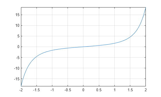
Plot Imaginary Error Function

Plot the imaginary error function on the interval from -2 to 2.

syms x
fplot(erfi(x),[-2,2])
grid on

Input Arguments

collapse all

`x` — Input
floating-point number | symbolic number | symbolic variable | symbolic expression | symbolic function | symbolic vector | symbolic matrix

Input, specified as a floating-point or symbolic number, variable,
expression, function, vector, or matrix.

More About

collapse all

The imaginary error function is defined as:

erfi(x)=−i erf(ix)=2π∫0xet2dt

Tips

erfi returns special values for these parameters:
- erfi(0) = 0
- erfi(inf) = inf
- erfi(-inf) = -inf
- erfi(i*inf) = i
- erfi(-i*inf) = -i

Version History

Introduced in R2013a

Источник

DiracDelta#

class sympy.functions.special.delta_functions.DiracDelta(arg, k=0)[source]#

The DiracDelta function and its derivatives.

Explanation

DiracDelta is not an ordinary function. It can be rigorously defined either
as a distribution or as a measure.

DiracDelta only makes sense in definite integrals, and in particular,
integrals of the form Integral(f(x)*DiracDelta(x - x0), (x, a, b)),
where it equals f(x0) if a <= x0 <= b and 0 otherwise. Formally,
DiracDelta acts in some ways like a function that is 0 everywhere except
at 0, but in many ways it also does not. It can often be useful to treat
DiracDelta in formal ways, building up and manipulating expressions with
delta functions (which may eventually be integrated), but care must be taken
to not treat it as a real function. SymPy’s oo is similar. It only
truly makes sense formally in certain contexts (such as integration limits),
but SymPy allows its use everywhere, and it tries to be consistent with
operations on it (like 1/oo), but it is easy to get into trouble and get
wrong results if oo is treated too much like a number. Similarly, if
DiracDelta is treated too much like a function, it is easy to get wrong or
nonsensical results.

DiracDelta function has the following properties:

(frac{d}{d x} theta(x) = delta(x))
(int_{-infty}^infty delta(x — a)f(x), dx = f(a)) and (int_{a-
epsilon}^{a+epsilon} delta(x — a)f(x), dx = f(a))
(delta(x) = 0) for all (x neq 0)
(delta(g(x)) = sum_i frac{delta(x — x_i)}{|g'(x_i)|}) where (x_i)
are the roots of (g)
(delta(-x) = delta(x))

Derivatives of k-th order of DiracDelta have the following properties:

(delta(x, k) = 0) for all (x neq 0)
(delta(-x, k) = -delta(x, k)) for odd (k)
(delta(-x, k) = delta(x, k)) for even (k)

Examples

>>> from sympy import DiracDelta, diff, pi
>>> from sympy.abc import x, y

>>> DiracDelta(x)
DiracDelta(x)
>>> DiracDelta(1)
0
>>> DiracDelta(-1)
0
>>> DiracDelta(pi)
0
>>> DiracDelta(x - 4).subs(x, 4)
DiracDelta(0)
>>> diff(DiracDelta(x))
DiracDelta(x, 1)
>>> diff(DiracDelta(x - 1), x, 2)
DiracDelta(x - 1, 2)
>>> diff(DiracDelta(x**2 - 1), x, 2)
2*(2*x**2*DiracDelta(x**2 - 1, 2) + DiracDelta(x**2 - 1, 1))
>>> DiracDelta(3*x).is_simple(x)
True
>>> DiracDelta(x**2).is_simple(x)
False
>>> DiracDelta((x**2 - 1)*y).expand(diracdelta=True, wrt=x)
DiracDelta(x - 1)/(2*Abs(y)) + DiracDelta(x + 1)/(2*Abs(y))

References

classmethod eval(arg, k=0)[source]#

Returns a simplified form or a value of DiracDelta depending on the
argument passed by the DiracDelta object.

Parameters:

k : integer

order of derivative

arg : argument passed to DiracDelta

Explanation

The eval() method is automatically called when the DiracDelta
class is about to be instantiated and it returns either some simplified
instance or the unevaluated instance depending on the argument passed.
In other words, eval() method is not needed to be called explicitly,
it is being called and evaluated once the object is called.

Examples

>>> from sympy import DiracDelta, S
>>> from sympy.abc import x

>>> DiracDelta(x)
DiracDelta(x)

>>> DiracDelta(-x, 1)
-DiracDelta(x, 1)

>>> DiracDelta(0)
DiracDelta(0)

>>> DiracDelta(S.NaN)
nan

>>> DiracDelta(x - 100).subs(x, 5)
0

>>> DiracDelta(x - 100).subs(x, 100)
DiracDelta(0)

fdiff(argindex=1)[source]#

Returns the first derivative of a DiracDelta Function.

Parameters:: argindex : integer

degree of derivative

Explanation

The difference between diff() and fdiff() is: diff() is the
user-level function and fdiff() is an object method. fdiff() is
a convenience method available in the Function class. It returns
the derivative of the function without considering the chain rule.
diff(function, x) calls Function._eval_derivative which in turn
calls fdiff() internally to compute the derivative of the function.

Examples

>>> from sympy import DiracDelta, diff
>>> from sympy.abc import x

>>> DiracDelta(x).fdiff()
DiracDelta(x, 1)

>>> DiracDelta(x, 1).fdiff()
DiracDelta(x, 2)

>>> DiracDelta(x**2 - 1).fdiff()
DiracDelta(x**2 - 1, 1)

>>> diff(DiracDelta(x, 1)).fdiff()
DiracDelta(x, 3)

is_simple(x)[source]#

Tells whether the argument(args[0]) of DiracDelta is a linear
expression in x.

Parameters:: x : can be a symbol

Examples

>>> from sympy import DiracDelta, cos
>>> from sympy.abc import x, y

>>> DiracDelta(x*y).is_simple(x)
True
>>> DiracDelta(x*y).is_simple(y)
True

>>> DiracDelta(x**2 + x - 2).is_simple(x)
False

>>> DiracDelta(cos(x)).is_simple(x)
False

Heaviside#

class sympy.functions.special.delta_functions.Heaviside(arg, H0=1 / 2)[source]#

Heaviside step function.

Explanation

The Heaviside step function has the following properties:

(frac{d}{d x} theta(x) = delta(x))
(theta(x) = begin{cases} 0 & text{for}: x < 0 \ frac{1}{2} &
text{for}: x = 0 \1 & text{for}: x > 0 end{cases})
(frac{d}{d x} max(x, 0) = theta(x))

Heaviside(x) is printed as (theta(x)) with the SymPy LaTeX printer.

The value at 0 is set differently in different fields. SymPy uses 1/2,
which is a convention from electronics and signal processing, and is
consistent with solving improper integrals by Fourier transform and
convolution.

To specify a different value of Heaviside at x=0, a second argument
can be given. Using Heaviside(x, nan) gives an expression that will
evaluate to nan for x=0.

Changed in version 1.9: Heaviside(0) now returns 1/2 (before: undefined)

Examples

>>> from sympy import Heaviside, nan
>>> from sympy.abc import x
>>> Heaviside(9)
1
>>> Heaviside(-9)
0
>>> Heaviside(0)
1/2
>>> Heaviside(0, nan)
nan
>>> (Heaviside(x) + 1).replace(Heaviside(x), Heaviside(x, 1))
Heaviside(x, 1) + 1

References

classmethod eval(arg, H0=1 / 2)[source]#

Returns a simplified form or a value of Heaviside depending on the
argument passed by the Heaviside object.

Parameters:

arg : argument passed by Heaviside object

H0 : value of Heaviside(0)

Explanation

The eval() method is automatically called when the Heaviside
class is about to be instantiated and it returns either some simplified
instance or the unevaluated instance depending on the argument passed.
In other words, eval() method is not needed to be called explicitly,
it is being called and evaluated once the object is called.

Examples

>>> from sympy import Heaviside, S
>>> from sympy.abc import x

>>> Heaviside(x)
Heaviside(x)

>>> Heaviside(x - 100).subs(x, 5)
0

>>> Heaviside(x - 100).subs(x, 105)
1

fdiff(argindex=1)[source]#

Returns the first derivative of a Heaviside Function.

Parameters:: argindex : integer

order of derivative

Examples

>>> from sympy import Heaviside, diff
>>> from sympy.abc import x

>>> Heaviside(x).fdiff()
DiracDelta(x)

>>> Heaviside(x**2 - 1).fdiff()
DiracDelta(x**2 - 1)

>>> diff(Heaviside(x)).fdiff()
DiracDelta(x, 1)

property pargs#: Args without default S.Half

Singularity Function#

class sympy.functions.special.singularity_functions.SingularityFunction(variable, offset, exponent)[source]#

Singularity functions are a class of discontinuous functions.

Explanation

Singularity functions take a variable, an offset, and an exponent as
arguments. These functions are represented using Macaulay brackets as:

SingularityFunction(x, a, n) := <x — a>^n

The singularity function will automatically evaluate to
Derivative(DiracDelta(x - a), x, -n - 1) if n < 0
and (x - a)**n*Heaviside(x - a) if n >= 0.

Examples

>>> from sympy import SingularityFunction, diff, Piecewise, DiracDelta, Heaviside, Symbol
>>> from sympy.abc import x, a, n
>>> SingularityFunction(x, a, n)
SingularityFunction(x, a, n)
>>> y = Symbol('y', positive=True)
>>> n = Symbol('n', nonnegative=True)
>>> SingularityFunction(y, -10, n)
(y + 10)**n
>>> y = Symbol('y', negative=True)
>>> SingularityFunction(y, 10, n)
0
>>> SingularityFunction(x, 4, -1).subs(x, 4)
oo
>>> SingularityFunction(x, 10, -2).subs(x, 10)
oo
>>> SingularityFunction(4, 1, 5)
243
>>> diff(SingularityFunction(x, 1, 5) + SingularityFunction(x, 1, 4), x)
4*SingularityFunction(x, 1, 3) + 5*SingularityFunction(x, 1, 4)
>>> diff(SingularityFunction(x, 4, 0), x, 2)
SingularityFunction(x, 4, -2)
>>> SingularityFunction(x, 4, 5).rewrite(Piecewise)
Piecewise(((x - 4)**5, x > 4), (0, True))
>>> expr = SingularityFunction(x, a, n)
>>> y = Symbol('y', positive=True)
>>> n = Symbol('n', nonnegative=True)
>>> expr.subs({x: y, a: -10, n: n})
(y + 10)**n

The methods rewrite(DiracDelta), rewrite(Heaviside), and
rewrite('HeavisideDiracDelta') returns the same output. One can use any
of these methods according to their choice.

>>> expr = SingularityFunction(x, 4, 5) + SingularityFunction(x, -3, -1) - SingularityFunction(x, 0, -2)
>>> expr.rewrite(Heaviside)
(x - 4)**5*Heaviside(x - 4) + DiracDelta(x + 3) - DiracDelta(x, 1)
>>> expr.rewrite(DiracDelta)
(x - 4)**5*Heaviside(x - 4) + DiracDelta(x + 3) - DiracDelta(x, 1)
>>> expr.rewrite('HeavisideDiracDelta')
(x - 4)**5*Heaviside(x - 4) + DiracDelta(x + 3) - DiracDelta(x, 1)

See also

DiracDelta, Heaviside

References

classmethod eval(variable, offset, exponent)[source]#

Returns a simplified form or a value of Singularity Function depending
on the argument passed by the object.

Explanation

The eval() method is automatically called when the
SingularityFunction class is about to be instantiated and it
returns either some simplified instance or the unevaluated instance
depending on the argument passed. In other words, eval() method is
not needed to be called explicitly, it is being called and evaluated
once the object is called.

Examples

>>> from sympy import SingularityFunction, Symbol, nan
>>> from sympy.abc import x, a, n
>>> SingularityFunction(x, a, n)
SingularityFunction(x, a, n)
>>> SingularityFunction(5, 3, 2)
4
>>> SingularityFunction(x, a, nan)
nan
>>> SingularityFunction(x, 3, 0).subs(x, 3)
1
>>> SingularityFunction(4, 1, 5)
243
>>> x = Symbol('x', positive = True)
>>> a = Symbol('a', negative = True)
>>> n = Symbol('n', nonnegative = True)
>>> SingularityFunction(x, a, n)
(-a + x)**n
>>> x = Symbol('x', negative = True)
>>> a = Symbol('a', positive = True)
>>> SingularityFunction(x, a, n)
0

fdiff(argindex=1)[source]#

Returns the first derivative of a DiracDelta Function.

Explanation

Gamma, Beta and related Functions#

class sympy.functions.special.gamma_functions.gamma(arg)[source]#

The gamma function

[Gamma(x) := int^{infty}_{0} t^{x-1} e^{-t} mathrm{d}t.]

Explanation

The gamma function implements the function which passes through the
values of the factorial function (i.e., (Gamma(n) = (n — 1)!) when n is
an integer). More generally, (Gamma(z)) is defined in the whole complex
plane except at the negative integers where there are simple poles.

Examples

>>> from sympy import S, I, pi, gamma
>>> from sympy.abc import x

Several special values are known:

>>> gamma(1)
1
>>> gamma(4)
6
>>> gamma(S(3)/2)
sqrt(pi)/2

The gamma function obeys the mirror symmetry:

>>> from sympy import conjugate
>>> conjugate(gamma(x))
gamma(conjugate(x))

Differentiation with respect to (x) is supported:

>>> from sympy import diff
>>> diff(gamma(x), x)
gamma(x)*polygamma(0, x)

Series expansion is also supported:

>>> from sympy import series
>>> series(gamma(x), x, 0, 3)
1/x - EulerGamma + x*(EulerGamma**2/2 + pi**2/12) + x**2*(-EulerGamma*pi**2/12 + polygamma(2, 1)/6 - EulerGamma**3/6) + O(x**3)

We can numerically evaluate the gamma function to arbitrary precision
on the whole complex plane:

>>> gamma(pi).evalf(40)
2.288037795340032417959588909060233922890
>>> gamma(1+I).evalf(20)
0.49801566811835604271 - 0.15494982830181068512*I

See also

lowergamma: Lower incomplete gamma function.
uppergamma: Upper incomplete gamma function.
polygamma: Polygamma function.
loggamma: Log Gamma function.
digamma: Digamma function.
trigamma: Trigamma function.
beta: Euler Beta function.

References

class sympy.functions.special.gamma_functions.loggamma(z)[source]#

The loggamma function implements the logarithm of the
gamma function (i.e., (logGamma(x))).

Examples

Several special values are known. For numerical integral
arguments we have:

>>> from sympy import loggamma
>>> loggamma(-2)
oo
>>> loggamma(0)
oo
>>> loggamma(1)
0
>>> loggamma(2)
0
>>> loggamma(3)
log(2)

And for symbolic values:

>>> from sympy import Symbol
>>> n = Symbol("n", integer=True, positive=True)
>>> loggamma(n)
log(gamma(n))
>>> loggamma(-n)
oo

For half-integral values:

>>> from sympy import S
>>> loggamma(S(5)/2)
log(3*sqrt(pi)/4)
>>> loggamma(n/2)
log(2**(1 - n)*sqrt(pi)*gamma(n)/gamma(n/2 + 1/2))

And general rational arguments:

>>> from sympy import expand_func
>>> L = loggamma(S(16)/3)
>>> expand_func(L).doit()
-5*log(3) + loggamma(1/3) + log(4) + log(7) + log(10) + log(13)
>>> L = loggamma(S(19)/4)
>>> expand_func(L).doit()
-4*log(4) + loggamma(3/4) + log(3) + log(7) + log(11) + log(15)
>>> L = loggamma(S(23)/7)
>>> expand_func(L).doit()
-3*log(7) + log(2) + loggamma(2/7) + log(9) + log(16)

The loggamma function has the following limits towards infinity:

>>> from sympy import oo
>>> loggamma(oo)
oo
>>> loggamma(-oo)
zoo

The loggamma function obeys the mirror symmetry
if (x in mathbb{C} setminus {-infty, 0}):

>>> from sympy.abc import x
>>> from sympy import conjugate
>>> conjugate(loggamma(x))
loggamma(conjugate(x))

Differentiation with respect to (x) is supported:

>>> from sympy import diff
>>> diff(loggamma(x), x)
polygamma(0, x)

Series expansion is also supported:

>>> from sympy import series
>>> series(loggamma(x), x, 0, 4).cancel()
-log(x) - EulerGamma*x + pi**2*x**2/12 + x**3*polygamma(2, 1)/6 + O(x**4)

We can numerically evaluate the gamma function to arbitrary precision
on the whole complex plane:

>>> from sympy import I
>>> loggamma(5).evalf(30)
3.17805383034794561964694160130
>>> loggamma(I).evalf(20)
-0.65092319930185633889 - 1.8724366472624298171*I

See also

gamma: Gamma function.
lowergamma: Lower incomplete gamma function.
uppergamma: Upper incomplete gamma function.
polygamma: Polygamma function.
digamma: Digamma function.
trigamma: Trigamma function.
beta: Euler Beta function.

References

class sympy.functions.special.gamma_functions.polygamma(n, z)[source]#

The function polygamma(n, z) returns log(gamma(z)).diff(n + 1).

Explanation

It is a meromorphic function on (mathbb{C}) and defined as the ((n+1))-th
derivative of the logarithm of the gamma function:

[psi^{(n)} (z) := frac{mathrm{d}^{n+1}}{mathrm{d} z^{n+1}} logGamma(z).]

Examples

Several special values are known:

>>> from sympy import S, polygamma
>>> polygamma(0, 1)
-EulerGamma
>>> polygamma(0, 1/S(2))
-2*log(2) - EulerGamma
>>> polygamma(0, 1/S(3))
-log(3) - sqrt(3)*pi/6 - EulerGamma - log(sqrt(3))
>>> polygamma(0, 1/S(4))
-pi/2 - log(4) - log(2) - EulerGamma
>>> polygamma(0, 2)
1 - EulerGamma
>>> polygamma(0, 23)
19093197/5173168 - EulerGamma

>>> from sympy import oo, I
>>> polygamma(0, oo)
oo
>>> polygamma(0, -oo)
oo
>>> polygamma(0, I*oo)
oo
>>> polygamma(0, -I*oo)
oo

Differentiation with respect to (x) is supported:

>>> from sympy import Symbol, diff
>>> x = Symbol("x")
>>> diff(polygamma(0, x), x)
polygamma(1, x)
>>> diff(polygamma(0, x), x, 2)
polygamma(2, x)
>>> diff(polygamma(0, x), x, 3)
polygamma(3, x)
>>> diff(polygamma(1, x), x)
polygamma(2, x)
>>> diff(polygamma(1, x), x, 2)
polygamma(3, x)
>>> diff(polygamma(2, x), x)
polygamma(3, x)
>>> diff(polygamma(2, x), x, 2)
polygamma(4, x)

>>> n = Symbol("n")
>>> diff(polygamma(n, x), x)
polygamma(n + 1, x)
>>> diff(polygamma(n, x), x, 2)
polygamma(n + 2, x)

We can rewrite polygamma functions in terms of harmonic numbers:

>>> from sympy import harmonic
>>> polygamma(0, x).rewrite(harmonic)
harmonic(x - 1) - EulerGamma
>>> polygamma(2, x).rewrite(harmonic)
2*harmonic(x - 1, 3) - 2*zeta(3)
>>> ni = Symbol("n", integer=True)
>>> polygamma(ni, x).rewrite(harmonic)
(-1)**(n + 1)*(-harmonic(x - 1, n + 1) + zeta(n + 1))*factorial(n)

See also

gamma: Gamma function.
lowergamma: Lower incomplete gamma function.
uppergamma: Upper incomplete gamma function.
loggamma: Log Gamma function.
digamma: Digamma function.
trigamma: Trigamma function.
beta: Euler Beta function.

References

class sympy.functions.special.gamma_functions.digamma(z)[source]#

The digamma function is the first derivative of the loggamma
function

[psi(x) := frac{mathrm{d}}{mathrm{d} z} logGamma(z)
= frac{Gamma'(z)}{Gamma(z) }.]

In this case, digamma(z) = polygamma(0, z).

Examples

>>> from sympy import digamma
>>> digamma(0)
zoo
>>> from sympy import Symbol
>>> z = Symbol('z')
>>> digamma(z)
polygamma(0, z)

To retain digamma as it is:

>>> digamma(0, evaluate=False)
digamma(0)
>>> digamma(z, evaluate=False)
digamma(z)

See also

gamma: Gamma function.
lowergamma: Lower incomplete gamma function.
uppergamma: Upper incomplete gamma function.
polygamma: Polygamma function.
loggamma: Log Gamma function.
trigamma: Trigamma function.
beta: Euler Beta function.

References

class sympy.functions.special.gamma_functions.trigamma(z)[source]#

The trigamma function is the second derivative of the loggamma
function

[psi^{(1)}(z) := frac{mathrm{d}^{2}}{mathrm{d} z^{2}} logGamma(z).]

In this case, trigamma(z) = polygamma(1, z).

Examples

>>> from sympy import trigamma
>>> trigamma(0)
zoo
>>> from sympy import Symbol
>>> z = Symbol('z')
>>> trigamma(z)
polygamma(1, z)

To retain trigamma as it is:

>>> trigamma(0, evaluate=False)
trigamma(0)
>>> trigamma(z, evaluate=False)
trigamma(z)

See also

gamma: Gamma function.
lowergamma: Lower incomplete gamma function.
uppergamma: Upper incomplete gamma function.
polygamma: Polygamma function.
loggamma: Log Gamma function.
digamma: Digamma function.
beta: Euler Beta function.

References

class sympy.functions.special.gamma_functions.uppergamma(a, z)[source]#

The upper incomplete gamma function.

Explanation

It can be defined as the meromorphic continuation of

[Gamma(s, x) := int_x^infty t^{s-1} e^{-t} mathrm{d}t = Gamma(s) — gamma(s, x).]

where (gamma(s, x)) is the lower incomplete gamma function,
lowergamma. This can be shown to be the same as

[Gamma(s, x) = Gamma(s) — frac{x^s}{s} {}_1F_1left({s atop s+1} middle| -xright),]

where ({}_1F_1) is the (confluent) hypergeometric function.

The upper incomplete gamma function is also essentially equivalent to the
generalized exponential integral:

[operatorname{E}_{n}(x) = int_{1}^{infty}{frac{e^{-xt}}{t^n} , dt} = x^{n-1}Gamma(1-n,x).]

Examples

>>> from sympy import uppergamma, S
>>> from sympy.abc import s, x
>>> uppergamma(s, x)
uppergamma(s, x)
>>> uppergamma(3, x)
2*(x**2/2 + x + 1)*exp(-x)
>>> uppergamma(-S(1)/2, x)
-2*sqrt(pi)*erfc(sqrt(x)) + 2*exp(-x)/sqrt(x)
>>> uppergamma(-2, x)
expint(3, x)/x**2

See also

gamma: Gamma function.
lowergamma: Lower incomplete gamma function.
polygamma: Polygamma function.
loggamma: Log Gamma function.
digamma: Digamma function.
trigamma: Trigamma function.
beta: Euler Beta function.

References

[R327]

Abramowitz, Milton; Stegun, Irene A., eds. (1965), Chapter 6,
Section 5, Handbook of Mathematical Functions with Formulas, Graphs,
and Mathematical Tables

class sympy.functions.special.gamma_functions.lowergamma(a, x)[source]#

The lower incomplete gamma function.

Explanation

It can be defined as the meromorphic continuation of

[gamma(s, x) := int_0^x t^{s-1} e^{-t} mathrm{d}t = Gamma(s) — Gamma(s, x).]

This can be shown to be the same as

[gamma(s, x) = frac{x^s}{s} {}_1F_1left({s atop s+1} middle| -xright),]

where ({}_1F_1) is the (confluent) hypergeometric function.

Examples

>>> from sympy import lowergamma, S
>>> from sympy.abc import s, x
>>> lowergamma(s, x)
lowergamma(s, x)
>>> lowergamma(3, x)
-2*(x**2/2 + x + 1)*exp(-x) + 2
>>> lowergamma(-S(1)/2, x)
-2*sqrt(pi)*erf(sqrt(x)) - 2*exp(-x)/sqrt(x)

See also

gamma: Gamma function.
uppergamma: Upper incomplete gamma function.
polygamma: Polygamma function.
loggamma: Log Gamma function.
digamma: Digamma function.
trigamma: Trigamma function.
beta: Euler Beta function.

References

[R333]

Abramowitz, Milton; Stegun, Irene A., eds. (1965), Chapter 6,
Section 5, Handbook of Mathematical Functions with Formulas, Graphs,
and Mathematical Tables

class sympy.functions.special.gamma_functions.multigamma(x, p)[source]#

The multivariate gamma function is a generalization of the gamma function

[Gamma_p(z) = pi^{p(p-1)/4}prod_{k=1}^p Gamma[z + (1 — k)/2].]

In a special case, multigamma(x, 1) = gamma(x).

Parameters:: p : order or dimension of the multivariate gamma function

Examples

>>> from sympy import S, multigamma
>>> from sympy import Symbol
>>> x = Symbol('x')
>>> p = Symbol('p', positive=True, integer=True)

>>> multigamma(x, p)
pi**(p*(p - 1)/4)*Product(gamma(-_k/2 + x + 1/2), (_k, 1, p))

Several special values are known:

>>> multigamma(1, 1)
1
>>> multigamma(4, 1)
6
>>> multigamma(S(3)/2, 1)
sqrt(pi)/2

Writing multigamma in terms of the gamma function:

>>> multigamma(x, 1)
gamma(x)

>>> multigamma(x, 2)
sqrt(pi)*gamma(x)*gamma(x - 1/2)

>>> multigamma(x, 3)
pi**(3/2)*gamma(x)*gamma(x - 1)*gamma(x - 1/2)

References

class sympy.functions.special.beta_functions.beta(x, y=None)[source]#

The beta integral is called the Eulerian integral of the first kind by
Legendre:

[mathrm{B}(x,y) int^{1}_{0} t^{x-1} (1-t)^{y-1} mathrm{d}t.]

Explanation

The Beta function or Euler’s first integral is closely associated
with the gamma function. The Beta function is often used in probability
theory and mathematical statistics. It satisfies properties like:

[begin{split}mathrm{B}(a,1) = frac{1}{a} \
mathrm{B}(a,b) = mathrm{B}(b,a) \
mathrm{B}(a,b) = frac{Gamma(a) Gamma(b)}{Gamma(a+b)}end{split}]

Therefore for integral values of (a) and (b):

[mathrm{B} = frac{(a-1)! (b-1)!}{(a+b-1)!}]

A special case of the Beta function when (x = y) is the
Central Beta function. It satisfies properties like:

[mathrm{B}(x) = 2^{1 — 2x}mathrm{B}(x, frac{1}{2})
mathrm{B}(x) = 2^{1 — 2x} cos(pi x) mathrm{B}(frac{1}{2} — x, x)
mathrm{B}(x) = int_{0}^{1} frac{t^x}{(1 + t)^{2x}} dt
mathrm{B}(x) = frac{2}{x} prod_{n = 1}^{infty} frac{n(n + 2x)}{(n + x)^2}]

Examples

>>> from sympy import I, pi
>>> from sympy.abc import x, y

The Beta function obeys the mirror symmetry:

>>> from sympy import beta, conjugate
>>> conjugate(beta(x, y))
beta(conjugate(x), conjugate(y))

Differentiation with respect to both (x) and (y) is supported:

>>> from sympy import beta, diff
>>> diff(beta(x, y), x)
(polygamma(0, x) - polygamma(0, x + y))*beta(x, y)

>>> diff(beta(x, y), y)
(polygamma(0, y) - polygamma(0, x + y))*beta(x, y)

>>> diff(beta(x), x)
2*(polygamma(0, x) - polygamma(0, 2*x))*beta(x, x)

We can numerically evaluate the Beta function to
arbitrary precision for any complex numbers x and y:

>>> from sympy import beta
>>> beta(pi).evalf(40)
0.02671848900111377452242355235388489324562

>>> beta(1 + I).evalf(20)
-0.2112723729365330143 - 0.7655283165378005676*I

See also

gamma: Gamma function.
uppergamma: Upper incomplete gamma function.
lowergamma: Lower incomplete gamma function.
polygamma: Polygamma function.
loggamma: Log Gamma function.
digamma: Digamma function.
trigamma: Trigamma function.

References

Error Functions and Fresnel Integrals#

class sympy.functions.special.error_functions.erf(arg)[source]#

The Gauss error function.

Explanation

This function is defined as:

[mathrm{erf}(x) = frac{2}{sqrt{pi}} int_0^x e^{-t^2} mathrm{d}t.]

Examples

>>> from sympy import I, oo, erf
>>> from sympy.abc import z

Several special values are known:

>>> erf(0)
0
>>> erf(oo)
1
>>> erf(-oo)
-1
>>> erf(I*oo)
oo*I
>>> erf(-I*oo)
-oo*I

In general one can pull out factors of -1 and (I) from the argument:

The error function obeys the mirror symmetry:

>>> from sympy import conjugate
>>> conjugate(erf(z))
erf(conjugate(z))

Differentiation with respect to (z) is supported:

>>> from sympy import diff
>>> diff(erf(z), z)
2*exp(-z**2)/sqrt(pi)

We can numerically evaluate the error function to arbitrary precision
on the whole complex plane:

>>> erf(4).evalf(30)
0.999999984582742099719981147840

>>> erf(-4*I).evalf(30)
-1296959.73071763923152794095062*I

See also

erfc: Complementary error function.
erfi: Imaginary error function.
erf2: Two-argument error function.
erfinv: Inverse error function.
erfcinv: Inverse Complementary error function.
erf2inv: Inverse two-argument error function.

References

inverse(argindex=1)[source]#: Returns the inverse of this function.

class sympy.functions.special.error_functions.erfc(arg)[source]#

Complementary Error Function.

Explanation

The function is defined as:

[mathrm{erfc}(x) = frac{2}{sqrt{pi}} int_x^infty e^{-t^2} mathrm{d}t]

Examples

>>> from sympy import I, oo, erfc
>>> from sympy.abc import z

Several special values are known:

>>> erfc(0)
1
>>> erfc(oo)
0
>>> erfc(-oo)
2
>>> erfc(I*oo)
-oo*I
>>> erfc(-I*oo)
oo*I

The error function obeys the mirror symmetry:

>>> from sympy import conjugate
>>> conjugate(erfc(z))
erfc(conjugate(z))

Differentiation with respect to (z) is supported:

>>> from sympy import diff
>>> diff(erfc(z), z)
-2*exp(-z**2)/sqrt(pi)

It also follows

We can numerically evaluate the complementary error function to arbitrary
precision on the whole complex plane:

>>> erfc(4).evalf(30)
0.0000000154172579002800188521596734869

>>> erfc(4*I).evalf(30)
1.0 - 1296959.73071763923152794095062*I

See also

erf: Gaussian error function.
erfi: Imaginary error function.
erf2: Two-argument error function.
erfinv: Inverse error function.
erfcinv: Inverse Complementary error function.
erf2inv: Inverse two-argument error function.

References

inverse(argindex=1)[source]#: Returns the inverse of this function.

class sympy.functions.special.error_functions.erfi(z)[source]#

Imaginary error function.

Explanation

The function erfi is defined as:

[mathrm{erfi}(x) = frac{2}{sqrt{pi}} int_0^x e^{t^2} mathrm{d}t]

Examples

>>> from sympy import I, oo, erfi
>>> from sympy.abc import z

Several special values are known:

>>> erfi(0)
0
>>> erfi(oo)
oo
>>> erfi(-oo)
-oo
>>> erfi(I*oo)
I
>>> erfi(-I*oo)
-I

In general one can pull out factors of -1 and (I) from the argument:

>>> from sympy import conjugate
>>> conjugate(erfi(z))
erfi(conjugate(z))

Differentiation with respect to (z) is supported:

>>> from sympy import diff
>>> diff(erfi(z), z)
2*exp(z**2)/sqrt(pi)

We can numerically evaluate the imaginary error function to arbitrary
precision on the whole complex plane:

>>> erfi(2).evalf(30)
18.5648024145755525987042919132

>>> erfi(-2*I).evalf(30)
-0.995322265018952734162069256367*I

See also

erf: Gaussian error function.
erfc: Complementary error function.
erf2: Two-argument error function.
erfinv: Inverse error function.
erfcinv: Inverse Complementary error function.
erf2inv: Inverse two-argument error function.

References

class sympy.functions.special.error_functions.erf2(x, y)[source]#

Two-argument error function.

Explanation

This function is defined as:

[mathrm{erf2}(x, y) = frac{2}{sqrt{pi}} int_x^y e^{-t^2} mathrm{d}t]

Examples

>>> from sympy import oo, erf2
>>> from sympy.abc import x, y

Several special values are known:

>>> erf2(0, 0)
0
>>> erf2(x, x)
0
>>> erf2(x, oo)
1 - erf(x)
>>> erf2(x, -oo)
-erf(x) - 1
>>> erf2(oo, y)
erf(y) - 1
>>> erf2(-oo, y)
erf(y) + 1

In general one can pull out factors of -1:

>>> erf2(-x, -y)
-erf2(x, y)

The error function obeys the mirror symmetry:

>>> from sympy import conjugate
>>> conjugate(erf2(x, y))
erf2(conjugate(x), conjugate(y))

Differentiation with respect to (x), (y) is supported:

>>> from sympy import diff
>>> diff(erf2(x, y), x)
-2*exp(-x**2)/sqrt(pi)
>>> diff(erf2(x, y), y)
2*exp(-y**2)/sqrt(pi)

See also

erf: Gaussian error function.
erfc: Complementary error function.
erfi: Imaginary error function.
erfinv: Inverse error function.
erfcinv: Inverse Complementary error function.
erf2inv: Inverse two-argument error function.

References

class sympy.functions.special.error_functions.erfinv(z)[source]#

Inverse Error Function. The erfinv function is defined as:

[mathrm{erf}(x) = y quad Rightarrow quad mathrm{erfinv}(y) = x]

Examples

>>> from sympy import erfinv
>>> from sympy.abc import x

Several special values are known:

>>> erfinv(0)
0
>>> erfinv(1)
oo

Differentiation with respect to (x) is supported:

>>> from sympy import diff
>>> diff(erfinv(x), x)
sqrt(pi)*exp(erfinv(x)**2)/2

We can numerically evaluate the inverse error function to arbitrary
precision on [-1, 1]:

>>> erfinv(0.2).evalf(30)
0.179143454621291692285822705344

See also

erf: Gaussian error function.
erfc: Complementary error function.
erfi: Imaginary error function.
erf2: Two-argument error function.
erfcinv: Inverse Complementary error function.
erf2inv: Inverse two-argument error function.

References

inverse(argindex=1)[source]#: Returns the inverse of this function.

class sympy.functions.special.error_functions.erfcinv(z)[source]#

Inverse Complementary Error Function. The erfcinv function is defined as:

[mathrm{erfc}(x) = y quad Rightarrow quad mathrm{erfcinv}(y) = x]

Examples

>>> from sympy import erfcinv
>>> from sympy.abc import x

Several special values are known:

>>> erfcinv(1)
0
>>> erfcinv(0)
oo

Differentiation with respect to (x) is supported:

>>> from sympy import diff
>>> diff(erfcinv(x), x)
-sqrt(pi)*exp(erfcinv(x)**2)/2

See also

erf: Gaussian error function.
erfc: Complementary error function.
erfi: Imaginary error function.
erf2: Two-argument error function.
erfinv: Inverse error function.
erf2inv: Inverse two-argument error function.

References

inverse(argindex=1)[source]#: Returns the inverse of this function.

class sympy.functions.special.error_functions.erf2inv(x, y)[source]#

Two-argument Inverse error function. The erf2inv function is defined as:

[mathrm{erf2}(x, w) = y quad Rightarrow quad mathrm{erf2inv}(x, y) = w]

Examples

>>> from sympy import erf2inv, oo
>>> from sympy.abc import x, y

Several special values are known:

>>> erf2inv(0, 0)
0
>>> erf2inv(1, 0)
1
>>> erf2inv(0, 1)
oo
>>> erf2inv(0, y)
erfinv(y)
>>> erf2inv(oo, y)
erfcinv(-y)

Differentiation with respect to (x) and (y) is supported:

>>> from sympy import diff
>>> diff(erf2inv(x, y), x)
exp(-x**2 + erf2inv(x, y)**2)
>>> diff(erf2inv(x, y), y)
sqrt(pi)*exp(erf2inv(x, y)**2)/2

See also

erf: Gaussian error function.
erfc: Complementary error function.
erfi: Imaginary error function.
erf2: Two-argument error function.
erfinv: Inverse error function.
erfcinv: Inverse complementary error function.

References

class sympy.functions.special.error_functions.FresnelIntegral(z)[source]#: Base class for the Fresnel integrals.

class sympy.functions.special.error_functions.fresnels(z)[source]#

Fresnel integral S.

Explanation

This function is defined by

[operatorname{S}(z) = int_0^z sin{frac{pi}{2} t^2} mathrm{d}t.]

It is an entire function.

Examples

>>> from sympy import I, oo, fresnels
>>> from sympy.abc import z

Several special values are known:

>>> fresnels(0)
0
>>> fresnels(oo)
1/2
>>> fresnels(-oo)
-1/2
>>> fresnels(I*oo)
-I/2
>>> fresnels(-I*oo)
I/2

In general one can pull out factors of -1 and (i) from the argument:

>>> fresnels(-z)
-fresnels(z)
>>> fresnels(I*z)
-I*fresnels(z)

The Fresnel S integral obeys the mirror symmetry
(overline{S(z)} = S(bar{z})):

>>> from sympy import conjugate
>>> conjugate(fresnels(z))
fresnels(conjugate(z))

Differentiation with respect to (z) is supported:

>>> from sympy import diff
>>> diff(fresnels(z), z)
sin(pi*z**2/2)

Defining the Fresnel functions via an integral:

>>> from sympy import integrate, pi, sin, expand_func
>>> integrate(sin(pi*z**2/2), z)
3*fresnels(z)*gamma(3/4)/(4*gamma(7/4))
>>> expand_func(integrate(sin(pi*z**2/2), z))
fresnels(z)

We can numerically evaluate the Fresnel integral to arbitrary precision
on the whole complex plane:

>>> fresnels(2).evalf(30)
0.343415678363698242195300815958

>>> fresnels(-2*I).evalf(30)
0.343415678363698242195300815958*I

See also

fresnelc: Fresnel cosine integral.

References

[R362]

The converging factors for the fresnel integrals
by John W. Wrench Jr. and Vicki Alley

class sympy.functions.special.error_functions.fresnelc(z)[source]#

Fresnel integral C.

Explanation

This function is defined by

[operatorname{C}(z) = int_0^z cos{frac{pi}{2} t^2} mathrm{d}t.]

It is an entire function.

Examples

>>> from sympy import I, oo, fresnelc
>>> from sympy.abc import z

Several special values are known:

>>> fresnelc(0)
0
>>> fresnelc(oo)
1/2
>>> fresnelc(-oo)
-1/2
>>> fresnelc(I*oo)
I/2
>>> fresnelc(-I*oo)
-I/2

In general one can pull out factors of -1 and (i) from the argument:

>>> fresnelc(-z)
-fresnelc(z)
>>> fresnelc(I*z)
I*fresnelc(z)

The Fresnel C integral obeys the mirror symmetry
(overline{C(z)} = C(bar{z})):

>>> from sympy import conjugate
>>> conjugate(fresnelc(z))
fresnelc(conjugate(z))

Differentiation with respect to (z) is supported:

>>> from sympy import diff
>>> diff(fresnelc(z), z)
cos(pi*z**2/2)

Defining the Fresnel functions via an integral:

>>> from sympy import integrate, pi, cos, expand_func
>>> integrate(cos(pi*z**2/2), z)
fresnelc(z)*gamma(1/4)/(4*gamma(5/4))
>>> expand_func(integrate(cos(pi*z**2/2), z))
fresnelc(z)

We can numerically evaluate the Fresnel integral to arbitrary precision
on the whole complex plane:

>>> fresnelc(2).evalf(30)
0.488253406075340754500223503357

>>> fresnelc(-2*I).evalf(30)
-0.488253406075340754500223503357*I

See also

fresnels: Fresnel sine integral.

References

[R367]

The converging factors for the fresnel integrals
by John W. Wrench Jr. and Vicki Alley

Exponential, Logarithmic and Trigonometric Integrals#

class sympy.functions.special.error_functions.Ei(z)[source]#

The classical exponential integral.

Explanation

For use in SymPy, this function is defined as

[operatorname{Ei}(x) = sum_{n=1}^infty frac{x^n}{n, n!}
+ log(x) + gamma,]

where (gamma) is the Euler-Mascheroni constant.

If (x) is a polar number, this defines an analytic function on the
Riemann surface of the logarithm. Otherwise this defines an analytic
function in the cut plane (mathbb{C} setminus (-infty, 0]).

Background

The name exponential integral comes from the following statement:

[operatorname{Ei}(x) = int_{-infty}^x frac{e^t}{t} mathrm{d}t]

If the integral is interpreted as a Cauchy principal value, this statement
holds for (x > 0) and (operatorname{Ei}(x)) as defined above.

Examples

>>> from sympy import Ei, polar_lift, exp_polar, I, pi
>>> from sympy.abc import x

This yields a real value:

>>> Ei(-1).n(chop=True)
-0.219383934395520

On the other hand the analytic continuation is not real:

>>> Ei(polar_lift(-1)).n(chop=True)
-0.21938393439552 + 3.14159265358979*I

The exponential integral has a logarithmic branch point at the origin:

>>> Ei(x*exp_polar(2*I*pi))
Ei(x) + 2*I*pi

Differentiation is supported:

>>> Ei(x).diff(x)
exp(x)/x

The exponential integral is related to many other special functions.
For example:

>>> from sympy import expint, Shi
>>> Ei(x).rewrite(expint)
-expint(1, x*exp_polar(I*pi)) - I*pi
>>> Ei(x).rewrite(Shi)
Chi(x) + Shi(x)

See also

expint: Generalised exponential integral.
E1: Special case of the generalised exponential integral.
li: Logarithmic integral.
Li: Offset logarithmic integral.
Si: Sine integral.
Ci: Cosine integral.
Shi: Hyperbolic sine integral.
Chi: Hyperbolic cosine integral.
uppergamma: Upper incomplete gamma function.

References

class sympy.functions.special.error_functions.expint(nu, z)[source]#

Generalized exponential integral.

Explanation

This function is defined as

[operatorname{E}_nu(z) = z^{nu — 1} Gamma(1 — nu, z),]

where (Gamma(1 — nu, z)) is the upper incomplete gamma function
(uppergamma).

Hence for (z) with positive real part we have

[operatorname{E}_nu(z)
= int_1^infty frac{e^{-zt}}{t^nu} mathrm{d}t,]

which explains the name.

The representation as an incomplete gamma function provides an analytic
continuation for (operatorname{E}_nu(z)). If (nu) is a
non-positive integer, the exponential integral is thus an unbranched
function of (z), otherwise there is a branch point at the origin.
Refer to the incomplete gamma function documentation for details of the
branching behavior.

Examples

>>> from sympy import expint, S
>>> from sympy.abc import nu, z

Differentiation is supported. Differentiation with respect to (z) further
explains the name: for integral orders, the exponential integral is an
iterated integral of the exponential function.

>>> expint(nu, z).diff(z)
-expint(nu - 1, z)

Differentiation with respect to (nu) has no classical expression:

>>> expint(nu, z).diff(nu)
-z**(nu - 1)*meijerg(((), (1, 1)), ((0, 0, 1 - nu), ()), z)

At non-postive integer orders, the exponential integral reduces to the
exponential function:

>>> expint(0, z)
exp(-z)/z
>>> expint(-1, z)
exp(-z)/z + exp(-z)/z**2

At half-integers it reduces to error functions:

>>> expint(S(1)/2, z)
sqrt(pi)*erfc(sqrt(z))/sqrt(z)

At positive integer orders it can be rewritten in terms of exponentials
and expint(1, z). Use expand_func() to do this:

>>> from sympy import expand_func
>>> expand_func(expint(5, z))
z**4*expint(1, z)/24 + (-z**3 + z**2 - 2*z + 6)*exp(-z)/24

The generalised exponential integral is essentially equivalent to the
incomplete gamma function:

>>> from sympy import uppergamma
>>> expint(nu, z).rewrite(uppergamma)
z**(nu - 1)*uppergamma(1 - nu, z)

As such it is branched at the origin:

>>> from sympy import exp_polar, pi, I
>>> expint(4, z*exp_polar(2*pi*I))
I*pi*z**3/3 + expint(4, z)
>>> expint(nu, z*exp_polar(2*pi*I))
z**(nu - 1)*(exp(2*I*pi*nu) - 1)*gamma(1 - nu) + expint(nu, z)

See also

Ei: Another related function called exponential integral.
E1: The classical case, returns expint(1, z).
li: Logarithmic integral.
Li: Offset logarithmic integral.
Si: Sine integral.
Ci: Cosine integral.
Shi: Hyperbolic sine integral.
Chi: Hyperbolic cosine integral.

uppergamma

References

sympy.functions.special.error_functions.E1(z)[source]#

Classical case of the generalized exponential integral.

Explanation

This is equivalent to expint(1, z).

Examples

>>> from sympy import E1
>>> E1(0)
expint(1, 0)

See also

Ei: Exponential integral.
expint: Generalised exponential integral.
li: Logarithmic integral.
Li: Offset logarithmic integral.
Si: Sine integral.
Ci: Cosine integral.
Shi: Hyperbolic sine integral.
Chi: Hyperbolic cosine integral.

class sympy.functions.special.error_functions.li(z)[source]#

The classical logarithmic integral.

Explanation

For use in SymPy, this function is defined as

[operatorname{li}(x) = int_0^x frac{1}{log(t)} mathrm{d}t ,.]

Examples

>>> from sympy import I, oo, li
>>> from sympy.abc import z

Several special values are known:

>>> li(0)
0
>>> li(1)
-oo
>>> li(oo)
oo

Differentiation with respect to (z) is supported:

>>> from sympy import diff
>>> diff(li(z), z)
1/log(z)

Defining the li function via an integral:
>>> from sympy import integrate
>>> integrate(li(z))
z*li(z) — Ei(2*log(z))

>>> integrate(li(z),z)
z*li(z) - Ei(2*log(z))

The logarithmic integral can also be defined in terms of Ei:

>>> from sympy import Ei
>>> li(z).rewrite(Ei)
Ei(log(z))
>>> diff(li(z).rewrite(Ei), z)
1/log(z)

We can numerically evaluate the logarithmic integral to arbitrary precision
on the whole complex plane (except the singular points):

>>> li(2).evalf(30)
1.04516378011749278484458888919

>>> li(2*I).evalf(30)
1.0652795784357498247001125598 + 3.08346052231061726610939702133*I

We can even compute Soldner’s constant by the help of mpmath:

>>> from mpmath import findroot
>>> findroot(li, 2)
1.45136923488338

Further transformations include rewriting li in terms of
the trigonometric integrals Si, Ci, Shi and Chi:

>>> from sympy import Si, Ci, Shi, Chi
>>> li(z).rewrite(Si)
-log(I*log(z)) - log(1/log(z))/2 + log(log(z))/2 + Ci(I*log(z)) + Shi(log(z))
>>> li(z).rewrite(Ci)
-log(I*log(z)) - log(1/log(z))/2 + log(log(z))/2 + Ci(I*log(z)) + Shi(log(z))
>>> li(z).rewrite(Shi)
-log(1/log(z))/2 + log(log(z))/2 + Chi(log(z)) - Shi(log(z))
>>> li(z).rewrite(Chi)
-log(1/log(z))/2 + log(log(z))/2 + Chi(log(z)) - Shi(log(z))

See also

Li: Offset logarithmic integral.
Ei: Exponential integral.
expint: Generalised exponential integral.
E1: Special case of the generalised exponential integral.
Si: Sine integral.
Ci: Cosine integral.
Shi: Hyperbolic sine integral.
Chi: Hyperbolic cosine integral.

References

class sympy.functions.special.error_functions.Li(z)[source]#

The offset logarithmic integral.

Explanation

For use in SymPy, this function is defined as

[operatorname{Li}(x) = operatorname{li}(x) — operatorname{li}(2)]

Examples

>>> from sympy import Li
>>> from sympy.abc import z

The following special value is known:

Differentiation with respect to (z) is supported:

>>> from sympy import diff
>>> diff(Li(z), z)
1/log(z)

The shifted logarithmic integral can be written in terms of (li(z)):

>>> from sympy import li
>>> Li(z).rewrite(li)
li(z) - li(2)

We can numerically evaluate the logarithmic integral to arbitrary precision
on the whole complex plane (except the singular points):

>>> Li(4).evalf(30)
1.92242131492155809316615998938

See also

li: Logarithmic integral.
Ei: Exponential integral.
expint: Generalised exponential integral.
E1: Special case of the generalised exponential integral.
Si: Sine integral.
Ci: Cosine integral.
Shi: Hyperbolic sine integral.
Chi: Hyperbolic cosine integral.

References

class sympy.functions.special.error_functions.Si(z)[source]#

Sine integral.

Explanation

This function is defined by

[operatorname{Si}(z) = int_0^z frac{sin{t}}{t} mathrm{d}t.]

It is an entire function.

Examples

>>> from sympy import Si
>>> from sympy.abc import z

The sine integral is an antiderivative of (sin(z)/z):

>>> Si(z).diff(z)
sin(z)/z

It is unbranched:

>>> from sympy import exp_polar, I, pi
>>> Si(z*exp_polar(2*I*pi))
Si(z)

Sine integral behaves much like ordinary sine under multiplication by I:

>>> Si(I*z)
I*Shi(z)
>>> Si(-z)
-Si(z)

It can also be expressed in terms of exponential integrals, but beware
that the latter is branched:

>>> from sympy import expint
>>> Si(z).rewrite(expint)
-I*(-expint(1, z*exp_polar(-I*pi/2))/2 +
     expint(1, z*exp_polar(I*pi/2))/2) + pi/2

It can be rewritten in the form of sinc function (by definition):

>>> from sympy import sinc
>>> Si(z).rewrite(sinc)
Integral(sinc(t), (t, 0, z))

See also

Ci: Cosine integral.
Shi: Hyperbolic sine integral.
Chi: Hyperbolic cosine integral.
Ei: Exponential integral.
expint: Generalised exponential integral.
sinc: unnormalized sinc function
E1: Special case of the generalised exponential integral.
li: Logarithmic integral.
Li: Offset logarithmic integral.

References

class sympy.functions.special.error_functions.Ci(z)[source]#

Cosine integral.

Explanation

This function is defined for positive (x) by

[operatorname{Ci}(x) = gamma + log{x}
+ int_0^x frac{cos{t} — 1}{t} mathrm{d}t
= -int_x^infty frac{cos{t}}{t} mathrm{d}t,]

where (gamma) is the Euler-Mascheroni constant.

We have

[operatorname{Ci}(z) =
-frac{operatorname{E}_1left(e^{ipi/2} zright)
+ operatorname{E}_1left(e^{-i pi/2} zright)}{2}]

which holds for all polar (z) and thus provides an analytic
continuation to the Riemann surface of the logarithm.

The formula also holds as stated
for (z in mathbb{C}) with (Re(z) > 0).
By lifting to the principal branch, we obtain an analytic function on the
cut complex plane.

Examples

>>> from sympy import Ci
>>> from sympy.abc import z

The cosine integral is a primitive of (cos(z)/z):

>>> Ci(z).diff(z)
cos(z)/z

It has a logarithmic branch point at the origin:

>>> from sympy import exp_polar, I, pi
>>> Ci(z*exp_polar(2*I*pi))
Ci(z) + 2*I*pi

The cosine integral behaves somewhat like ordinary (cos) under
multiplication by (i):

>>> from sympy import polar_lift
>>> Ci(polar_lift(I)*z)
Chi(z) + I*pi/2
>>> Ci(polar_lift(-1)*z)
Ci(z) + I*pi

It can also be expressed in terms of exponential integrals:

>>> from sympy import expint
>>> Ci(z).rewrite(expint)
-expint(1, z*exp_polar(-I*pi/2))/2 - expint(1, z*exp_polar(I*pi/2))/2

See also

Si: Sine integral.
Shi: Hyperbolic sine integral.
Chi: Hyperbolic cosine integral.
Ei: Exponential integral.
expint: Generalised exponential integral.
E1: Special case of the generalised exponential integral.
li: Logarithmic integral.
Li: Offset logarithmic integral.

References

class sympy.functions.special.error_functions.Shi(z)[source]#

Sinh integral.

Explanation

This function is defined by

[operatorname{Shi}(z) = int_0^z frac{sinh{t}}{t} mathrm{d}t.]

It is an entire function.

Examples

>>> from sympy import Shi
>>> from sympy.abc import z

The Sinh integral is a primitive of (sinh(z)/z):

>>> Shi(z).diff(z)
sinh(z)/z

It is unbranched:

>>> from sympy import exp_polar, I, pi
>>> Shi(z*exp_polar(2*I*pi))
Shi(z)

The (sinh) integral behaves much like ordinary (sinh) under
multiplication by (i):

>>> Shi(I*z)
I*Si(z)
>>> Shi(-z)
-Shi(z)

It can also be expressed in terms of exponential integrals, but beware
that the latter is branched:

>>> from sympy import expint
>>> Shi(z).rewrite(expint)
expint(1, z)/2 - expint(1, z*exp_polar(I*pi))/2 - I*pi/2

See also

Si: Sine integral.
Ci: Cosine integral.
Chi: Hyperbolic cosine integral.
Ei: Exponential integral.
expint: Generalised exponential integral.
E1: Special case of the generalised exponential integral.
li: Logarithmic integral.
Li: Offset logarithmic integral.

References

class sympy.functions.special.error_functions.Chi(z)[source]#

Cosh integral.

Explanation

This function is defined for positive (x) by

[operatorname{Chi}(x) = gamma + log{x}
+ int_0^x frac{cosh{t} — 1}{t} mathrm{d}t,]

where (gamma) is the Euler-Mascheroni constant.

We have

[operatorname{Chi}(z) = operatorname{Ci}left(e^{i pi/2}zright)
— ifrac{pi}{2},]

which holds for all polar (z) and thus provides an analytic
continuation to the Riemann surface of the logarithm.
By lifting to the principal branch we obtain an analytic function on the
cut complex plane.

Examples

>>> from sympy import Chi
>>> from sympy.abc import z

The (cosh) integral is a primitive of (cosh(z)/z):

>>> Chi(z).diff(z)
cosh(z)/z

It has a logarithmic branch point at the origin:

>>> from sympy import exp_polar, I, pi
>>> Chi(z*exp_polar(2*I*pi))
Chi(z) + 2*I*pi

The (cosh) integral behaves somewhat like ordinary (cosh) under
multiplication by (i):

>>> from sympy import polar_lift
>>> Chi(polar_lift(I)*z)
Ci(z) + I*pi/2
>>> Chi(polar_lift(-1)*z)
Chi(z) + I*pi

It can also be expressed in terms of exponential integrals:

>>> from sympy import expint
>>> Chi(z).rewrite(expint)
-expint(1, z)/2 - expint(1, z*exp_polar(I*pi))/2 - I*pi/2

See also

Si: Sine integral.
Ci: Cosine integral.
Shi: Hyperbolic sine integral.
Ei: Exponential integral.
expint: Generalised exponential integral.
E1: Special case of the generalised exponential integral.
li: Logarithmic integral.
Li: Offset logarithmic integral.

References

Bessel Type Functions#

class sympy.functions.special.bessel.BesselBase(nu, z)[source]#

Abstract base class for Bessel-type functions.

This class is meant to reduce code duplication.
All Bessel-type functions can 1) be differentiated, with the derivatives
expressed in terms of similar functions, and 2) be rewritten in terms
of other Bessel-type functions.

Here, Bessel-type functions are assumed to have one complex parameter.

To use this base class, define class attributes _a and _b such that
2*F_n' = -_a*F_{n+1} + b*F_{n-1}.

property argument#: The argument of the Bessel-type function.

property order#: The order of the Bessel-type function.

class sympy.functions.special.bessel.besselj(nu, z)[source]#

Bessel function of the first kind.

Explanation

The Bessel (J) function of order (nu) is defined to be the function
satisfying Bessel’s differential equation

[z^2 frac{mathrm{d}^2 w}{mathrm{d}z^2}
+ z frac{mathrm{d}w}{mathrm{d}z} + (z^2 — nu^2) w = 0,]

with Laurent expansion

[J_nu(z) = z^nu left(frac{1}{Gamma(nu + 1) 2^nu} + O(z^2) right),]

if (nu) is not a negative integer. If (nu=-n in mathbb{Z}_{<0})
is a negative integer, then the definition is

[J_{-n}(z) = (-1)^n J_n(z).]

Examples

Create a Bessel function object:

>>> from sympy import besselj, jn
>>> from sympy.abc import z, n
>>> b = besselj(n, z)

Differentiate it:

>>> b.diff(z)
besselj(n - 1, z)/2 - besselj(n + 1, z)/2

Rewrite in terms of spherical Bessel functions:

>>> b.rewrite(jn)
sqrt(2)*sqrt(z)*jn(n - 1/2, z)/sqrt(pi)

Access the parameter and argument:

>>> b.order
n
>>> b.argument
z

See also

bessely, besseli, besselk

References

[R385]

Abramowitz, Milton; Stegun, Irene A., eds. (1965), “Chapter 9”,
Handbook of Mathematical Functions with Formulas, Graphs, and
Mathematical Tables

[R386]

Luke, Y. L. (1969), The Special Functions and Their
Approximations, Volume 1

class sympy.functions.special.bessel.bessely(nu, z)[source]#

Bessel function of the second kind.

Explanation

The Bessel (Y) function of order (nu) is defined as

[Y_nu(z) = lim_{mu to nu} frac{J_mu(z) cos(pi mu)
— J_{-mu}(z)}{sin(pi mu)},]

where (J_mu(z)) is the Bessel function of the first kind.

It is a solution to Bessel’s equation, and linearly independent from
(J_nu).

Examples

>>> from sympy import bessely, yn
>>> from sympy.abc import z, n
>>> b = bessely(n, z)
>>> b.diff(z)
bessely(n - 1, z)/2 - bessely(n + 1, z)/2
>>> b.rewrite(yn)
sqrt(2)*sqrt(z)*yn(n - 1/2, z)/sqrt(pi)

See also

besselj, besseli, besselk

References

class sympy.functions.special.bessel.besseli(nu, z)[source]#

Modified Bessel function of the first kind.

Explanation

The Bessel (I) function is a solution to the modified Bessel equation

[z^2 frac{mathrm{d}^2 w}{mathrm{d}z^2}
+ z frac{mathrm{d}w}{mathrm{d}z} + (z^2 + nu^2)^2 w = 0.]

It can be defined as

[I_nu(z) = i^{-nu} J_nu(iz),]

where (J_nu(z)) is the Bessel function of the first kind.

Examples

>>> from sympy import besseli
>>> from sympy.abc import z, n
>>> besseli(n, z).diff(z)
besseli(n - 1, z)/2 + besseli(n + 1, z)/2

See also

besselj, bessely, besselk

References

class sympy.functions.special.bessel.besselk(nu, z)[source]#

Modified Bessel function of the second kind.

Explanation

The Bessel (K) function of order (nu) is defined as

[K_nu(z) = lim_{mu to nu} frac{pi}{2}
frac{I_{-mu}(z) -I_mu(z)}{sin(pi mu)},]

where (I_mu(z)) is the modified Bessel function of the first kind.

It is a solution of the modified Bessel equation, and linearly independent
from (Y_nu).

Examples

>>> from sympy import besselk
>>> from sympy.abc import z, n
>>> besselk(n, z).diff(z)
-besselk(n - 1, z)/2 - besselk(n + 1, z)/2

See also

besselj, besseli, bessely

References

class sympy.functions.special.bessel.hankel1(nu, z)[source]#

Hankel function of the first kind.

Explanation

This function is defined as

[H_nu^{(1)} = J_nu(z) + iY_nu(z),]

where (J_nu(z)) is the Bessel function of the first kind, and
(Y_nu(z)) is the Bessel function of the second kind.

It is a solution to Bessel’s equation.

Examples

>>> from sympy import hankel1
>>> from sympy.abc import z, n
>>> hankel1(n, z).diff(z)
hankel1(n - 1, z)/2 - hankel1(n + 1, z)/2

See also

hankel2, besselj, bessely

References

class sympy.functions.special.bessel.hankel2(nu, z)[source]#

Hankel function of the second kind.

Explanation

This function is defined as

[H_nu^{(2)} = J_nu(z) — iY_nu(z),]

where (J_nu(z)) is the Bessel function of the first kind, and
(Y_nu(z)) is the Bessel function of the second kind.

It is a solution to Bessel’s equation, and linearly independent from
(H_nu^{(1)}).

Examples

>>> from sympy import hankel2
>>> from sympy.abc import z, n
>>> hankel2(n, z).diff(z)
hankel2(n - 1, z)/2 - hankel2(n + 1, z)/2

See also

hankel1, besselj, bessely

References

class sympy.functions.special.bessel.jn(nu, z)[source]#

Spherical Bessel function of the first kind.

Explanation

This function is a solution to the spherical Bessel equation

[z^2 frac{mathrm{d}^2 w}{mathrm{d}z^2}
+ 2z frac{mathrm{d}w}{mathrm{d}z} + (z^2 — nu(nu + 1)) w = 0.]

It can be defined as

[j_nu(z) = sqrt{frac{pi}{2z}} J_{nu + frac{1}{2}}(z),]

where (J_nu(z)) is the Bessel function of the first kind.

The spherical Bessel functions of integral order are
calculated using the formula:

[j_n(z) = f_n(z) sin{z} + (-1)^{n+1} f_{-n-1}(z) cos{z},]

where the coefficients (f_n(z)) are available as
sympy.polys.orthopolys.spherical_bessel_fn().

Examples

>>> from sympy import Symbol, jn, sin, cos, expand_func, besselj, bessely
>>> z = Symbol("z")
>>> nu = Symbol("nu", integer=True)
>>> print(expand_func(jn(0, z)))
sin(z)/z
>>> expand_func(jn(1, z)) == sin(z)/z**2 - cos(z)/z
True
>>> expand_func(jn(3, z))
(-6/z**2 + 15/z**4)*sin(z) + (1/z - 15/z**3)*cos(z)
>>> jn(nu, z).rewrite(besselj)
sqrt(2)*sqrt(pi)*sqrt(1/z)*besselj(nu + 1/2, z)/2
>>> jn(nu, z).rewrite(bessely)
(-1)**nu*sqrt(2)*sqrt(pi)*sqrt(1/z)*bessely(-nu - 1/2, z)/2
>>> jn(2, 5.2+0.3j).evalf(20)
0.099419756723640344491 - 0.054525080242173562897*I

See also

besselj, bessely, besselk, yn

References

class sympy.functions.special.bessel.yn(nu, z)[source]#

Spherical Bessel function of the second kind.

Explanation

This function is another solution to the spherical Bessel equation, and
linearly independent from (j_n). It can be defined as

[y_nu(z) = sqrt{frac{pi}{2z}} Y_{nu + frac{1}{2}}(z),]

where (Y_nu(z)) is the Bessel function of the second kind.

For integral orders (n), (y_n) is calculated using the formula:

[y_n(z) = (-1)^{n+1} j_{-n-1}(z)]

Examples

>>> from sympy import Symbol, yn, sin, cos, expand_func, besselj, bessely
>>> z = Symbol("z")
>>> nu = Symbol("nu", integer=True)
>>> print(expand_func(yn(0, z)))
-cos(z)/z
>>> expand_func(yn(1, z)) == -cos(z)/z**2-sin(z)/z
True
>>> yn(nu, z).rewrite(besselj)
(-1)**(nu + 1)*sqrt(2)*sqrt(pi)*sqrt(1/z)*besselj(-nu - 1/2, z)/2
>>> yn(nu, z).rewrite(bessely)
sqrt(2)*sqrt(pi)*sqrt(1/z)*bessely(nu + 1/2, z)/2
>>> yn(2, 5.2+0.3j).evalf(20)
0.18525034196069722536 + 0.014895573969924817587*I

See also

besselj, bessely, besselk, jn

References

sympy.functions.special.bessel.jn_zeros(n, k, method=‘sympy’, dps=15)[source]#

Zeros of the spherical Bessel function of the first kind.

Parameters:

n : integer

order of Bessel function

k : integer

number of zeros to return

Explanation

This returns an array of zeros of (jn) up to the (k)-th zero.

method = “sympy”: uses mpmath.besseljzero
method = “scipy”: uses the
SciPy’s sph_jn
and
newton
to find all
roots, which is faster than computing the zeros using a general
numerical solver, but it requires SciPy and only works with low
precision floating point numbers. (The function used with
method=”sympy” is a recent addition to mpmath; before that a general
solver was used.)

Examples

>>> from sympy import jn_zeros
>>> jn_zeros(2, 4, dps=5)
[5.7635, 9.095, 12.323, 15.515]

See also

jn, yn, besselj, besselk, bessely

class sympy.functions.special.bessel.marcumq(m, a, b)[source]#

The Marcum Q-function.

Explanation

The Marcum Q-function is defined by the meromorphic continuation of

[Q_m(a, b) = a^{- m + 1} int_{b}^{infty} x^{m} e^{- frac{a^{2}}{2} — frac{x^{2}}{2}} I_{m — 1}left(a xright), dx]

Examples

>>> from sympy import marcumq
>>> from sympy.abc import m, a, b
>>> marcumq(m, a, b)
marcumq(m, a, b)

Special values:

>>> marcumq(m, 0, b)
uppergamma(m, b**2/2)/gamma(m)
>>> marcumq(0, 0, 0)
0
>>> marcumq(0, a, 0)
1 - exp(-a**2/2)
>>> marcumq(1, a, a)
1/2 + exp(-a**2)*besseli(0, a**2)/2
>>> marcumq(2, a, a)
1/2 + exp(-a**2)*besseli(0, a**2)/2 + exp(-a**2)*besseli(1, a**2)

Differentiation with respect to (a) and (b) is supported:

>>> from sympy import diff
>>> diff(marcumq(m, a, b), a)
a*(-marcumq(m, a, b) + marcumq(m + 1, a, b))
>>> diff(marcumq(m, a, b), b)
-a**(1 - m)*b**m*exp(-a**2/2 - b**2/2)*besseli(m - 1, a*b)

References

Airy Functions#

class sympy.functions.special.bessel.AiryBase(*args)[source]#

Abstract base class for Airy functions.

This class is meant to reduce code duplication.

class sympy.functions.special.bessel.airyai(arg)[source]#

The Airy function (operatorname{Ai}) of the first kind.

Explanation

The Airy function (operatorname{Ai}(z)) is defined to be the function
satisfying Airy’s differential equation

[frac{mathrm{d}^2 w(z)}{mathrm{d}z^2} — z w(z) = 0.]

Equivalently, for real (z)

[operatorname{Ai}(z) := frac{1}{pi}
int_0^infty cosleft(frac{t^3}{3} + z tright) mathrm{d}t.]

Examples

Create an Airy function object:

>>> from sympy import airyai
>>> from sympy.abc import z

Several special values are known:

>>> airyai(0)
3**(1/3)/(3*gamma(2/3))
>>> from sympy import oo
>>> airyai(oo)
0
>>> airyai(-oo)
0

The Airy function obeys the mirror symmetry:

>>> from sympy import conjugate
>>> conjugate(airyai(z))
airyai(conjugate(z))

Differentiation with respect to (z) is supported:

>>> from sympy import diff
>>> diff(airyai(z), z)
airyaiprime(z)
>>> diff(airyai(z), z, 2)
z*airyai(z)

Series expansion is also supported:

>>> from sympy import series
>>> series(airyai(z), z, 0, 3)
3**(5/6)*gamma(1/3)/(6*pi) - 3**(1/6)*z*gamma(2/3)/(2*pi) + O(z**3)

We can numerically evaluate the Airy function to arbitrary precision
on the whole complex plane:

>>> airyai(-2).evalf(50)
0.22740742820168557599192443603787379946077222541710

Rewrite (operatorname{Ai}(z)) in terms of hypergeometric functions:

>>> from sympy import hyper
>>> airyai(z).rewrite(hyper)
-3**(2/3)*z*hyper((), (4/3,), z**3/9)/(3*gamma(1/3)) + 3**(1/3)*hyper((), (2/3,), z**3/9)/(3*gamma(2/3))

See also

airybi: Airy function of the second kind.
airyaiprime: Derivative of the Airy function of the first kind.
airybiprime: Derivative of the Airy function of the second kind.

References

class sympy.functions.special.bessel.airybi(arg)[source]#

The Airy function (operatorname{Bi}) of the second kind.

Explanation

The Airy function (operatorname{Bi}(z)) is defined to be the function
satisfying Airy’s differential equation

[frac{mathrm{d}^2 w(z)}{mathrm{d}z^2} — z w(z) = 0.]

Equivalently, for real (z)

[operatorname{Bi}(z) := frac{1}{pi}
int_0^infty
expleft(-frac{t^3}{3} + z tright)
+ sinleft(frac{t^3}{3} + z tright) mathrm{d}t.]

Examples

Create an Airy function object:

>>> from sympy import airybi
>>> from sympy.abc import z

Several special values are known:

>>> airybi(0)
3**(5/6)/(3*gamma(2/3))
>>> from sympy import oo
>>> airybi(oo)
oo
>>> airybi(-oo)
0

The Airy function obeys the mirror symmetry:

>>> from sympy import conjugate
>>> conjugate(airybi(z))
airybi(conjugate(z))

Differentiation with respect to (z) is supported:

>>> from sympy import diff
>>> diff(airybi(z), z)
airybiprime(z)
>>> diff(airybi(z), z, 2)
z*airybi(z)

Series expansion is also supported:

>>> from sympy import series
>>> series(airybi(z), z, 0, 3)
3**(1/3)*gamma(1/3)/(2*pi) + 3**(2/3)*z*gamma(2/3)/(2*pi) + O(z**3)

We can numerically evaluate the Airy function to arbitrary precision
on the whole complex plane:

>>> airybi(-2).evalf(50)
-0.41230258795639848808323405461146104203453483447240

Rewrite (operatorname{Bi}(z)) in terms of hypergeometric functions:

>>> from sympy import hyper
>>> airybi(z).rewrite(hyper)
3**(1/6)*z*hyper((), (4/3,), z**3/9)/gamma(1/3) + 3**(5/6)*hyper((), (2/3,), z**3/9)/(3*gamma(2/3))

See also

airyai: Airy function of the first kind.
airyaiprime: Derivative of the Airy function of the first kind.
airybiprime: Derivative of the Airy function of the second kind.

References

class sympy.functions.special.bessel.airyaiprime(arg)[source]#

The derivative (operatorname{Ai}^prime) of the Airy function of the first
kind.

Explanation

The Airy function (operatorname{Ai}^prime(z)) is defined to be the
function

[operatorname{Ai}^prime(z) := frac{mathrm{d} operatorname{Ai}(z)}{mathrm{d} z}.]

Examples

Create an Airy function object:

>>> from sympy import airyaiprime
>>> from sympy.abc import z

>>> airyaiprime(z)
airyaiprime(z)

Several special values are known:

>>> airyaiprime(0)
-3**(2/3)/(3*gamma(1/3))
>>> from sympy import oo
>>> airyaiprime(oo)
0

The Airy function obeys the mirror symmetry:

>>> from sympy import conjugate
>>> conjugate(airyaiprime(z))
airyaiprime(conjugate(z))

Differentiation with respect to (z) is supported:

>>> from sympy import diff
>>> diff(airyaiprime(z), z)
z*airyai(z)
>>> diff(airyaiprime(z), z, 2)
z*airyaiprime(z) + airyai(z)

Series expansion is also supported:

>>> from sympy import series
>>> series(airyaiprime(z), z, 0, 3)
-3**(2/3)/(3*gamma(1/3)) + 3**(1/3)*z**2/(6*gamma(2/3)) + O(z**3)

We can numerically evaluate the Airy function to arbitrary precision
on the whole complex plane:

>>> airyaiprime(-2).evalf(50)
0.61825902074169104140626429133247528291577794512415

Rewrite (operatorname{Ai}^prime(z)) in terms of hypergeometric functions:

>>> from sympy import hyper
>>> airyaiprime(z).rewrite(hyper)
3**(1/3)*z**2*hyper((), (5/3,), z**3/9)/(6*gamma(2/3)) - 3**(2/3)*hyper((), (1/3,), z**3/9)/(3*gamma(1/3))

See also

airyai: Airy function of the first kind.
airybi: Airy function of the second kind.
airybiprime: Derivative of the Airy function of the second kind.

References

class sympy.functions.special.bessel.airybiprime(arg)[source]#

The derivative (operatorname{Bi}^prime) of the Airy function of the first
kind.

Explanation

The Airy function (operatorname{Bi}^prime(z)) is defined to be the
function

[operatorname{Bi}^prime(z) := frac{mathrm{d} operatorname{Bi}(z)}{mathrm{d} z}.]

Examples

Create an Airy function object:

>>> from sympy import airybiprime
>>> from sympy.abc import z

>>> airybiprime(z)
airybiprime(z)

Several special values are known:

>>> airybiprime(0)
3**(1/6)/gamma(1/3)
>>> from sympy import oo
>>> airybiprime(oo)
oo
>>> airybiprime(-oo)
0

The Airy function obeys the mirror symmetry:

>>> from sympy import conjugate
>>> conjugate(airybiprime(z))
airybiprime(conjugate(z))

Differentiation with respect to (z) is supported:

>>> from sympy import diff
>>> diff(airybiprime(z), z)
z*airybi(z)
>>> diff(airybiprime(z), z, 2)
z*airybiprime(z) + airybi(z)

Series expansion is also supported:

>>> from sympy import series
>>> series(airybiprime(z), z, 0, 3)
3**(1/6)/gamma(1/3) + 3**(5/6)*z**2/(6*gamma(2/3)) + O(z**3)

We can numerically evaluate the Airy function to arbitrary precision
on the whole complex plane:

>>> airybiprime(-2).evalf(50)
0.27879516692116952268509756941098324140300059345163

Rewrite (operatorname{Bi}^prime(z)) in terms of hypergeometric functions:

>>> from sympy import hyper
>>> airybiprime(z).rewrite(hyper)
3**(5/6)*z**2*hyper((), (5/3,), z**3/9)/(6*gamma(2/3)) + 3**(1/6)*hyper((), (1/3,), z**3/9)/gamma(1/3)

See also

airyai: Airy function of the first kind.
airybi: Airy function of the second kind.
airyaiprime: Derivative of the Airy function of the first kind.

References

B-Splines#

sympy.functions.special.bsplines.bspline_basis(d, knots, n, x)[source]#

The (n)-th B-spline at (x) of degree (d) with knots.

Parameters:

d : integer

degree of bspline

knots : list of integer values

list of knots points of bspline

n : integer

(n)-th B-spline

x : symbol

Explanation

B-Splines are piecewise polynomials of degree (d). They are defined on a
set of knots, which is a sequence of integers or floats.

Examples

The 0th degree splines have a value of 1 on a single interval:

>>> from sympy import bspline_basis
>>> from sympy.abc import x
>>> d = 0
>>> knots = tuple(range(5))
>>> bspline_basis(d, knots, 0, x)
Piecewise((1, (x >= 0) & (x <= 1)), (0, True))

For a given (d, knots) there are len(knots)-d-1 B-splines
defined, that are indexed by n (starting at 0).

Here is an example of a cubic B-spline:

>>> bspline_basis(3, tuple(range(5)), 0, x)
Piecewise((x**3/6, (x >= 0) & (x <= 1)),
          (-x**3/2 + 2*x**2 - 2*x + 2/3,
          (x >= 1) & (x <= 2)),
          (x**3/2 - 4*x**2 + 10*x - 22/3,
          (x >= 2) & (x <= 3)),
          (-x**3/6 + 2*x**2 - 8*x + 32/3,
          (x >= 3) & (x <= 4)),
          (0, True))

By repeating knot points, you can introduce discontinuities in the
B-splines and their derivatives:

>>> d = 1
>>> knots = (0, 0, 2, 3, 4)
>>> bspline_basis(d, knots, 0, x)
Piecewise((1 - x/2, (x >= 0) & (x <= 2)), (0, True))

It is quite time consuming to construct and evaluate B-splines. If
you need to evaluate a B-spline many times, it is best to lambdify them
first:

>>> from sympy import lambdify
>>> d = 3
>>> knots = tuple(range(10))
>>> b0 = bspline_basis(d, knots, 0, x)
>>> f = lambdify(x, b0)
>>> y = f(0.5)

See also

bspline_basis_set

References

sympy.functions.special.bsplines.bspline_basis_set(d, knots, x)[source]#

Return the len(knots)-d-1 B-splines at x of degree d
with knots.

Parameters:

d : integer

degree of bspline

knots : list of integers

list of knots points of bspline

x : symbol

Explanation

This function returns a list of piecewise polynomials that are the
len(knots)-d-1 B-splines of degree d for the given knots.
This function calls bspline_basis(d, knots, n, x) for different
values of n.

Examples

>>> from sympy import bspline_basis_set
>>> from sympy.abc import x
>>> d = 2
>>> knots = range(5)
>>> splines = bspline_basis_set(d, knots, x)
>>> splines
[Piecewise((x**2/2, (x >= 0) & (x <= 1)),
           (-x**2 + 3*x - 3/2, (x >= 1) & (x <= 2)),
           (x**2/2 - 3*x + 9/2, (x >= 2) & (x <= 3)),
           (0, True)),
Piecewise((x**2/2 - x + 1/2, (x >= 1) & (x <= 2)),
          (-x**2 + 5*x - 11/2, (x >= 2) & (x <= 3)),
          (x**2/2 - 4*x + 8, (x >= 3) & (x <= 4)),
          (0, True))]

sympy.functions.special.bsplines.interpolating_spline(d, x, X, Y)[source]#

Return spline of degree d, passing through the given X
and Y values.

Parameters:

d : integer

Degree of Bspline strictly greater than equal to one

x : symbol

X : list of strictly increasing integer values

list of X coordinates through which the spline passes

Y : list of strictly increasing integer values

list of Y coordinates through which the spline passes

Explanation

This function returns a piecewise function such that each part is
a polynomial of degree not greater than d. The value of d
must be 1 or greater and the values of X must be strictly
increasing.

Examples

>>> from sympy import interpolating_spline
>>> from sympy.abc import x
>>> interpolating_spline(1, x, [1, 2, 4, 7], [3, 6, 5, 7])
Piecewise((3*x, (x >= 1) & (x <= 2)),
        (7 - x/2, (x >= 2) & (x <= 4)),
        (2*x/3 + 7/3, (x >= 4) & (x <= 7)))
>>> interpolating_spline(3, x, [-2, 0, 1, 3, 4], [4, 2, 1, 1, 3])
Piecewise((7*x**3/117 + 7*x**2/117 - 131*x/117 + 2, (x >= -2) & (x <= 1)),
        (10*x**3/117 - 2*x**2/117 - 122*x/117 + 77/39, (x >= 1) & (x <= 4)))

Riemann Zeta and Related Functions#

class sympy.functions.special.zeta_functions.zeta(z, a_=None)[source]#

Hurwitz zeta function (or Riemann zeta function).

Explanation

For (operatorname{Re}(a) > 0) and (operatorname{Re}(s) > 1), this
function is defined as

[zeta(s, a) = sum_{n=0}^infty frac{1}{(n + a)^s},]

where the standard choice of argument for (n + a) is used. For fixed
(a) with (operatorname{Re}(a) > 0) the Hurwitz zeta function admits a
meromorphic continuation to all of (mathbb{C}), it is an unbranched
function with a simple pole at (s = 1).

Analytic continuation to other (a) is possible under some circumstances,
but this is not typically done.

The Hurwitz zeta function is a special case of the Lerch transcendent:

[zeta(s, a) = Phi(1, s, a).]

This formula defines an analytic continuation for all possible values of
(s) and (a) (also (operatorname{Re}(a) < 0)), see the documentation of
lerchphi for a description of the branching behavior.

If no value is passed for (a), by this function assumes a default value
of (a = 1), yielding the Riemann zeta function.

Examples

For (a = 1) the Hurwitz zeta function reduces to the famous Riemann
zeta function:

[zeta(s, 1) = zeta(s) = sum_{n=1}^infty frac{1}{n^s}.]

>>> from sympy import zeta
>>> from sympy.abc import s
>>> zeta(s, 1)
zeta(s)
>>> zeta(s)
zeta(s)

The Riemann zeta function can also be expressed using the Dirichlet eta
function:

>>> from sympy import dirichlet_eta
>>> zeta(s).rewrite(dirichlet_eta)
dirichlet_eta(s)/(1 - 2**(1 - s))

The Riemann zeta function at positive even integer and negative odd integer
values is related to the Bernoulli numbers:

>>> zeta(2)
pi**2/6
>>> zeta(4)
pi**4/90
>>> zeta(-1)
-1/12

The specific formulae are:

[zeta(2n) = (-1)^{n+1} frac{B_{2n} (2pi)^{2n}}{2(2n)!}]

[zeta(-n) = -frac{B_{n+1}}{n+1}]

At negative even integers the Riemann zeta function is zero:

No closed-form expressions are known at positive odd integers, but
numerical evaluation is possible:

>>> zeta(3).n()
1.20205690315959

The derivative of (zeta(s, a)) with respect to (a) can be computed:

>>> from sympy.abc import a
>>> zeta(s, a).diff(a)
-s*zeta(s + 1, a)

However the derivative with respect to (s) has no useful closed form
expression:

>>> zeta(s, a).diff(s)
Derivative(zeta(s, a), s)

The Hurwitz zeta function can be expressed in terms of the Lerch
transcendent, lerchphi:

>>> from sympy import lerchphi
>>> zeta(s, a).rewrite(lerchphi)
lerchphi(1, s, a)

References

class sympy.functions.special.zeta_functions.dirichlet_eta(s)[source]#

Dirichlet eta function.

Explanation

For (operatorname{Re}(s) > 0), this function is defined as

[eta(s) = sum_{n=1}^infty frac{(-1)^{n-1}}{n^s}.]

It admits a unique analytic continuation to all of (mathbb{C}).
It is an entire, unbranched function.

Examples

The Dirichlet eta function is closely related to the Riemann zeta function:

>>> from sympy import dirichlet_eta, zeta
>>> from sympy.abc import s
>>> dirichlet_eta(s).rewrite(zeta)
(1 - 2**(1 - s))*zeta(s)

References

class sympy.functions.special.zeta_functions.polylog(s, z)[source]#

Polylogarithm function.

Explanation

For (|z| < 1) and (s in mathbb{C}), the polylogarithm is
defined by

[operatorname{Li}_s(z) = sum_{n=1}^infty frac{z^n}{n^s},]

where the standard branch of the argument is used for (n). It admits
an analytic continuation which is branched at (z=1) (notably not on the
sheet of initial definition), (z=0) and (z=infty).

The name polylogarithm comes from the fact that for (s=1), the
polylogarithm is related to the ordinary logarithm (see examples), and that

[operatorname{Li}_{s+1}(z) =
int_0^z frac{operatorname{Li}_s(t)}{t} mathrm{d}t.]

The polylogarithm is a special case of the Lerch transcendent:

[operatorname{Li}_{s}(z) = z Phi(z, s, 1).]

Examples

For (z in {0, 1, -1}), the polylogarithm is automatically expressed
using other functions:

>>> from sympy import polylog
>>> from sympy.abc import s
>>> polylog(s, 0)
0
>>> polylog(s, 1)
zeta(s)
>>> polylog(s, -1)
-dirichlet_eta(s)

If (s) is a negative integer, (0) or (1), the polylogarithm can be
expressed using elementary functions. This can be done using
expand_func():

>>> from sympy import expand_func
>>> from sympy.abc import z
>>> expand_func(polylog(1, z))
-log(1 - z)
>>> expand_func(polylog(0, z))
z/(1 - z)

The derivative with respect to (z) can be computed in closed form:

>>> polylog(s, z).diff(z)
polylog(s - 1, z)/z

The polylogarithm can be expressed in terms of the lerch transcendent:

>>> from sympy import lerchphi
>>> polylog(s, z).rewrite(lerchphi)
z*lerchphi(z, s, 1)

class sympy.functions.special.zeta_functions.lerchphi(*args)[source]#

Lerch transcendent (Lerch phi function).

Explanation

For (operatorname{Re}(a) > 0), (|z| < 1) and (s in mathbb{C}), the
Lerch transcendent is defined as

[Phi(z, s, a) = sum_{n=0}^infty frac{z^n}{(n + a)^s},]

where the standard branch of the argument is used for (n + a),
and by analytic continuation for other values of the parameters.

A commonly used related function is the Lerch zeta function, defined by

[L(q, s, a) = Phi(e^{2pi i q}, s, a).]

Analytic Continuation and Branching Behavior

It can be shown that

[Phi(z, s, a) = zPhi(z, s, a+1) + a^{-s}.]

This provides the analytic continuation to (operatorname{Re}(a) le 0).

Assume now (operatorname{Re}(a) > 0). The integral representation

[Phi_0(z, s, a) = int_0^infty frac{t^{s-1} e^{-at}}{1 — ze^{-t}}
frac{mathrm{d}t}{Gamma(s)}]

provides an analytic continuation to (mathbb{C} — [1, infty)).
Finally, for (x in (1, infty)) we find

[lim_{epsilon to 0^+} Phi_0(x + iepsilon, s, a)
-lim_{epsilon to 0^+} Phi_0(x — iepsilon, s, a)
= frac{2pi i log^{s-1}{x}}{x^a Gamma(s)},]

using the standard branch for both (log{x}) and
(log{log{x}}) (a branch of (log{log{x}}) is needed to
evaluate (log{x}^{s-1})).
This concludes the analytic continuation. The Lerch transcendent is thus
branched at (z in {0, 1, infty}) and
(a in mathbb{Z}_{le 0}). For fixed (z, a) outside these
branch points, it is an entire function of (s).

Examples

The Lerch transcendent is a fairly general function, for this reason it does
not automatically evaluate to simpler functions. Use expand_func() to
achieve this.

If (z=1), the Lerch transcendent reduces to the Hurwitz zeta function:

>>> from sympy import lerchphi, expand_func
>>> from sympy.abc import z, s, a
>>> expand_func(lerchphi(1, s, a))
zeta(s, a)

More generally, if (z) is a root of unity, the Lerch transcendent
reduces to a sum of Hurwitz zeta functions:

>>> expand_func(lerchphi(-1, s, a))
zeta(s, a/2)/2**s - zeta(s, a/2 + 1/2)/2**s

If (a=1), the Lerch transcendent reduces to the polylogarithm:

>>> expand_func(lerchphi(z, s, 1))
polylog(s, z)/z

More generally, if (a) is rational, the Lerch transcendent reduces
to a sum of polylogarithms:

>>> from sympy import S
>>> expand_func(lerchphi(z, s, S(1)/2))
2**(s - 1)*(polylog(s, sqrt(z))/sqrt(z) -
            polylog(s, sqrt(z)*exp_polar(I*pi))/sqrt(z))
>>> expand_func(lerchphi(z, s, S(3)/2))
-2**s/z + 2**(s - 1)*(polylog(s, sqrt(z))/sqrt(z) -
                      polylog(s, sqrt(z)*exp_polar(I*pi))/sqrt(z))/z

The derivatives with respect to (z) and (a) can be computed in
closed form:

>>> lerchphi(z, s, a).diff(z)
(-a*lerchphi(z, s, a) + lerchphi(z, s - 1, a))/z
>>> lerchphi(z, s, a).diff(a)
-s*lerchphi(z, s + 1, a)

References

[R418]

Bateman, H.; Erdelyi, A. (1953), Higher Transcendental Functions,
Vol. I, New York: McGraw-Hill. Section 1.11.

class sympy.functions.special.zeta_functions.stieltjes(n, a=None)[source]#

Represents Stieltjes constants, (gamma_{k}) that occur in
Laurent Series expansion of the Riemann zeta function.

Examples

>>> from sympy import stieltjes
>>> from sympy.abc import n, m
>>> stieltjes(n)
stieltjes(n)

The zero’th stieltjes constant:

>>> stieltjes(0)
EulerGamma
>>> stieltjes(0, 1)
EulerGamma

For generalized stieltjes constants:

>>> stieltjes(n, m)
stieltjes(n, m)

Constants are only defined for integers >= 0:

References

Hypergeometric Functions#

class sympy.functions.special.hyper.hyper(ap, bq, z)[source]#

The generalized hypergeometric function is defined by a series where
the ratios of successive terms are a rational function of the summation
index. When convergent, it is continued analytically to the largest
possible domain.

Explanation

The hypergeometric function depends on two vectors of parameters, called
the numerator parameters (a_p), and the denominator parameters
(b_q). It also has an argument (z). The series definition is

[begin{split}{}_pF_qleft(begin{matrix} a_1, cdots, a_p \ b_1, cdots, b_q end{matrix}
middle| z right)
= sum_{n=0}^infty frac{(a_1)_n cdots (a_p)_n}{(b_1)_n cdots (b_q)_n}
frac{z^n}{n!},end{split}]

where ((a)_n = (a)(a+1)cdots(a+n-1)) denotes the rising factorial.

If one of the (b_q) is a non-positive integer then the series is
undefined unless one of the (a_p) is a larger (i.e., smaller in
magnitude) non-positive integer. If none of the (b_q) is a
non-positive integer and one of the (a_p) is a non-positive
integer, then the series reduces to a polynomial. To simplify the
following discussion, we assume that none of the (a_p) or
(b_q) is a non-positive integer. For more details, see the
references.

The series converges for all (z) if (p le q), and thus
defines an entire single-valued function in this case. If (p =
q+1) the series converges for (|z| < 1), and can be continued
analytically into a half-plane. If (p > q+1) the series is
divergent for all (z).

Please note the hypergeometric function constructor currently does not
check if the parameters actually yield a well-defined function.

Examples

The parameters (a_p) and (b_q) can be passed as arbitrary
iterables, for example:

>>> from sympy import hyper
>>> from sympy.abc import x, n, a
>>> hyper((1, 2, 3), [3, 4], x)
hyper((1, 2, 3), (3, 4), x)

There is also pretty printing (it looks better using Unicode):

>>> from sympy import pprint
>>> pprint(hyper((1, 2, 3), [3, 4], x), use_unicode=False)
  _
 |_  /1, 2, 3 |  
 |   |        | x|
3  2   3, 4  |  /

The parameters must always be iterables, even if they are vectors of
length one or zero:

>>> hyper((1, ), [], x)
hyper((1,), (), x)

But of course they may be variables (but if they depend on (x) then you
should not expect much implemented functionality):

>>> hyper((n, a), (n**2,), x)
hyper((n, a), (n**2,), x)

The hypergeometric function generalizes many named special functions.
The function hyperexpand() tries to express a hypergeometric function
using named special functions. For example:

>>> from sympy import hyperexpand
>>> hyperexpand(hyper([], [], x))
exp(x)

You can also use expand_func():

>>> from sympy import expand_func
>>> expand_func(x*hyper([1, 1], [2], -x))
log(x + 1)

More examples:

>>> from sympy import S
>>> hyperexpand(hyper([], [S(1)/2], -x**2/4))
cos(x)
>>> hyperexpand(x*hyper([S(1)/2, S(1)/2], [S(3)/2], x**2))
asin(x)

We can also sometimes hyperexpand() parametric functions:

>>> from sympy.abc import a
>>> hyperexpand(hyper([-a], [], x))
(1 - x)**a

References

[R422]

Luke, Y. L. (1969), The Special Functions and Their Approximations,
Volume 1

property ap#: Numerator parameters of the hypergeometric function.

property argument#: Argument of the hypergeometric function.

property bq#: Denominator parameters of the hypergeometric function.

property convergence_statement#: Return a condition on z under which the series converges.

property eta#: A quantity related to the convergence of the series.

property radius_of_convergence#

Compute the radius of convergence of the defining series.

Explanation

Note that even if this is not oo, the function may still be
evaluated outside of the radius of convergence by analytic
continuation. But if this is zero, then the function is not actually
defined anywhere else.

Examples

>>> from sympy import hyper
>>> from sympy.abc import z
>>> hyper((1, 2), [3], z).radius_of_convergence
1
>>> hyper((1, 2, 3), [4], z).radius_of_convergence
0
>>> hyper((1, 2), (3, 4), z).radius_of_convergence
oo

class sympy.functions.special.hyper.meijerg(*args)[source]#

The Meijer G-function is defined by a Mellin-Barnes type integral that
resembles an inverse Mellin transform. It generalizes the hypergeometric
functions.

Explanation

The Meijer G-function depends on four sets of parameters. There are
“numerator parameters”
(a_1, ldots, a_n) and (a_{n+1}, ldots, a_p), and there are
“denominator parameters”
(b_1, ldots, b_m) and (b_{m+1}, ldots, b_q).
Confusingly, it is traditionally denoted as follows (note the position
of (m), (n), (p), (q), and how they relate to the lengths of the four
parameter vectors):

[begin{split}G_{p,q}^{m,n} left(begin{matrix}a_1, cdots, a_n & a_{n+1}, cdots, a_p \
b_1, cdots, b_m & b_{m+1}, cdots, b_q
end{matrix} middle| z right).end{split}]

However, in SymPy the four parameter vectors are always available
separately (see examples), so that there is no need to keep track of the
decorating sub- and super-scripts on the G symbol.

The G function is defined as the following integral:

[frac{1}{2 pi i} int_L frac{prod_{j=1}^m Gamma(b_j — s)
prod_{j=1}^n Gamma(1 — a_j + s)}{prod_{j=m+1}^q Gamma(1- b_j +s)
prod_{j=n+1}^p Gamma(a_j — s)} z^s mathrm{d}s,]

where (Gamma(z)) is the gamma function. There are three possible
contours which we will not describe in detail here (see the references).
If the integral converges along more than one of them, the definitions
agree. The contours all separate the poles of (Gamma(1-a_j+s))
from the poles of (Gamma(b_k-s)), so in particular the G function
is undefined if (a_j — b_k in mathbb{Z}_{>0}) for some
(j le n) and (k le m).

The conditions under which one of the contours yields a convergent integral
are complicated and we do not state them here, see the references.

Please note currently the Meijer G-function constructor does not check any
convergence conditions.

Examples

You can pass the parameters either as four separate vectors:

>>> from sympy import meijerg, Tuple, pprint
>>> from sympy.abc import x, a
>>> pprint(meijerg((1, 2), (a, 4), (5,), [], x), use_unicode=False)
 __1, 2 /1, 2  a, 4 |  
/__     |           | x|
_|4, 1  5         |  /

Or as two nested vectors:

>>> pprint(meijerg([(1, 2), (3, 4)], ([5], Tuple()), x), use_unicode=False)
 __1, 2 /1, 2  3, 4 |  
/__     |           | x|
_|4, 1  5         |  /

As with the hypergeometric function, the parameters may be passed as
arbitrary iterables. Vectors of length zero and one also have to be
passed as iterables. The parameters need not be constants, but if they
depend on the argument then not much implemented functionality should be
expected.

All the subvectors of parameters are available:

>>> from sympy import pprint
>>> g = meijerg([1], [2], [3], [4], x)
>>> pprint(g, use_unicode=False)
 __1, 1 /1  2 |  
/__     |     | x|
_|2, 2 3  4 |  /
>>> g.an
(1,)
>>> g.ap
(1, 2)
>>> g.aother
(2,)
>>> g.bm
(3,)
>>> g.bq
(3, 4)
>>> g.bother
(4,)

The Meijer G-function generalizes the hypergeometric functions.
In some cases it can be expressed in terms of hypergeometric functions,
using Slater’s theorem. For example:

>>> from sympy import hyperexpand
>>> from sympy.abc import a, b, c
>>> hyperexpand(meijerg([a], [], [c], [b], x), allow_hyper=True)
x**c*gamma(-a + c + 1)*hyper((-a + c + 1,),
                             (-b + c + 1,), -x)/gamma(-b + c + 1)

Thus the Meijer G-function also subsumes many named functions as special
cases. You can use expand_func() or hyperexpand() to (try to)
rewrite a Meijer G-function in terms of named special functions. For
example:

>>> from sympy import expand_func, S
>>> expand_func(meijerg([[],[]], [[0],[]], -x))
exp(x)
>>> hyperexpand(meijerg([[],[]], [[S(1)/2],[0]], (x/2)**2))
sin(x)/sqrt(pi)

References

[R424]

Luke, Y. L. (1969), The Special Functions and Their Approximations,
Volume 1

property an#: First set of numerator parameters.

property aother#: Second set of numerator parameters.

property ap#: Combined numerator parameters.

property argument#: Argument of the Meijer G-function.

property bm#: First set of denominator parameters.

property bother#: Second set of denominator parameters.

property bq#: Combined denominator parameters.

property delta#: A quantity related to the convergence region of the integral,
c.f. references.

get_period()[source]#

Return a number (P) such that (G(x*exp(I*P)) == G(x)).

Examples

>>> from sympy import meijerg, pi, S
>>> from sympy.abc import z

>>> meijerg([1], [], [], [], z).get_period()
2*pi
>>> meijerg([pi], [], [], [], z).get_period()
oo
>>> meijerg([1, 2], [], [], [], z).get_period()
oo
>>> meijerg([1,1], [2], [1, S(1)/2, S(1)/3], [1], z).get_period()
12*pi

integrand(s)[source]#: Get the defining integrand D(s).

property is_number#: Returns true if expression has numeric data only.

property nu#: A quantity related to the convergence region of the integral,
c.f. references.

class sympy.functions.special.hyper.appellf1(a, b1, b2, c, x, y)[source]#

This is the Appell hypergeometric function of two variables as:

[F_1(a,b_1,b_2,c,x,y) = sum_{m=0}^{infty} sum_{n=0}^{infty}
frac{(a)_{m+n} (b_1)_m (b_2)_n}{(c)_{m+n}}
frac{x^m y^n}{m! n!}.]

Examples

>>> from sympy import appellf1, symbols
>>> x, y, a, b1, b2, c = symbols('x y a b1 b2 c')
>>> appellf1(2., 1., 6., 4., 5., 6.)
0.0063339426292673
>>> appellf1(12., 12., 6., 4., 0.5, 0.12)
172870711.659936
>>> appellf1(40, 2, 6, 4, 15, 60)
appellf1(40, 2, 6, 4, 15, 60)
>>> appellf1(20., 12., 10., 3., 0.5, 0.12)
15605338197184.4
>>> appellf1(40, 2, 6, 4, x, y)
appellf1(40, 2, 6, 4, x, y)
>>> appellf1(a, b1, b2, c, x, y)
appellf1(a, b1, b2, c, x, y)

References

Elliptic integrals#

class sympy.functions.special.elliptic_integrals.elliptic_k(m)[source]#

The complete elliptic integral of the first kind, defined by

[K(m) = Fleft(tfrac{pi}{2}middle| mright)]

where (Fleft(zmiddle| mright)) is the Legendre incomplete
elliptic integral of the first kind.

Explanation

The function (K(m)) is a single-valued function on the complex
plane with branch cut along the interval ((1, infty)).

Note that our notation defines the incomplete elliptic integral
in terms of the parameter (m) instead of the elliptic modulus
(eccentricity) (k).
In this case, the parameter (m) is defined as (m=k^2).

Examples

>>> from sympy import elliptic_k, I
>>> from sympy.abc import m
>>> elliptic_k(0)
pi/2
>>> elliptic_k(1.0 + I)
1.50923695405127 + 0.625146415202697*I
>>> elliptic_k(m).series(n=3)
pi/2 + pi*m/8 + 9*pi*m**2/128 + O(m**3)

References

class sympy.functions.special.elliptic_integrals.elliptic_f(z, m)[source]#

The Legendre incomplete elliptic integral of the first
kind, defined by

[Fleft(zmiddle| mright) =
int_0^z frac{dt}{sqrt{1 — m sin^2 t}}]

Explanation

This function reduces to a complete elliptic integral of
the first kind, (K(m)), when (z = pi/2).

Examples

>>> from sympy import elliptic_f, I
>>> from sympy.abc import z, m
>>> elliptic_f(z, m).series(z)
z + z**5*(3*m**2/40 - m/30) + m*z**3/6 + O(z**6)
>>> elliptic_f(3.0 + I/2, 1.0 + I)
2.909449841483 + 1.74720545502474*I

References

class sympy.functions.special.elliptic_integrals.elliptic_e(m, z=None)[source]#

Called with two arguments (z) and (m), evaluates the
incomplete elliptic integral of the second kind, defined by

[Eleft(zmiddle| mright) = int_0^z sqrt{1 — m sin^2 t} dt]

Called with a single argument (m), evaluates the Legendre complete
elliptic integral of the second kind

[E(m) = Eleft(tfrac{pi}{2}middle| mright)]

Explanation

The function (E(m)) is a single-valued function on the complex
plane with branch cut along the interval ((1, infty)).

Examples

>>> from sympy import elliptic_e, I
>>> from sympy.abc import z, m
>>> elliptic_e(z, m).series(z)
z + z**5*(-m**2/40 + m/30) - m*z**3/6 + O(z**6)
>>> elliptic_e(m).series(n=4)
pi/2 - pi*m/8 - 3*pi*m**2/128 - 5*pi*m**3/512 + O(m**4)
>>> elliptic_e(1 + I, 2 - I/2).n()
1.55203744279187 + 0.290764986058437*I
>>> elliptic_e(0)
pi/2
>>> elliptic_e(2.0 - I)
0.991052601328069 + 0.81879421395609*I

References

class sympy.functions.special.elliptic_integrals.elliptic_pi(n, m, z=None)[source]#

Called with three arguments (n), (z) and (m), evaluates the
Legendre incomplete elliptic integral of the third kind, defined by

[Pileft(n; zmiddle| mright) = int_0^z frac{dt}
{left(1 — n sin^2 tright) sqrt{1 — m sin^2 t}}]

Called with two arguments (n) and (m), evaluates the complete
elliptic integral of the third kind:

[Pileft(nmiddle| mright) =
Pileft(n; tfrac{pi}{2}middle| mright)]

Explanation

Examples

>>> from sympy import elliptic_pi, I
>>> from sympy.abc import z, n, m
>>> elliptic_pi(n, z, m).series(z, n=4)
z + z**3*(m/6 + n/3) + O(z**4)
>>> elliptic_pi(0.5 + I, 1.0 - I, 1.2)
2.50232379629182 - 0.760939574180767*I
>>> elliptic_pi(0, 0)
pi/2
>>> elliptic_pi(1.0 - I/3, 2.0 + I)
3.29136443417283 + 0.32555634906645*I

References

Mathieu Functions#

class sympy.functions.special.mathieu_functions.MathieuBase(*args)[source]#

Abstract base class for Mathieu functions.

This class is meant to reduce code duplication.

class sympy.functions.special.mathieu_functions.mathieus(a, q, z)[source]#

The Mathieu Sine function (S(a,q,z)).

Explanation

This function is one solution of the Mathieu differential equation:

[y(x)^{primeprime} + (a — 2 q cos(2 x)) y(x) = 0]

The other solution is the Mathieu Cosine function.

Examples

>>> from sympy import diff, mathieus
>>> from sympy.abc import a, q, z

>>> mathieus(a, q, z)
mathieus(a, q, z)

>>> mathieus(a, 0, z)
sin(sqrt(a)*z)

>>> diff(mathieus(a, q, z), z)
mathieusprime(a, q, z)

See also

mathieuc: Mathieu cosine function.
mathieusprime: Derivative of Mathieu sine function.
mathieucprime: Derivative of Mathieu cosine function.

References

class sympy.functions.special.mathieu_functions.mathieuc(a, q, z)[source]#

The Mathieu Cosine function (C(a,q,z)).

Explanation

This function is one solution of the Mathieu differential equation:

[y(x)^{primeprime} + (a — 2 q cos(2 x)) y(x) = 0]

The other solution is the Mathieu Sine function.

Examples

>>> from sympy import diff, mathieuc
>>> from sympy.abc import a, q, z

>>> mathieuc(a, q, z)
mathieuc(a, q, z)

>>> mathieuc(a, 0, z)
cos(sqrt(a)*z)

>>> diff(mathieuc(a, q, z), z)
mathieucprime(a, q, z)

See also

mathieus: Mathieu sine function
mathieusprime: Derivative of Mathieu sine function
mathieucprime: Derivative of Mathieu cosine function

References

class sympy.functions.special.mathieu_functions.mathieusprime(a, q, z)[source]#

The derivative (S^{prime}(a,q,z)) of the Mathieu Sine function.

Explanation

This function is one solution of the Mathieu differential equation:

[y(x)^{primeprime} + (a — 2 q cos(2 x)) y(x) = 0]

The other solution is the Mathieu Cosine function.

Examples

>>> from sympy import diff, mathieusprime
>>> from sympy.abc import a, q, z

>>> mathieusprime(a, q, z)
mathieusprime(a, q, z)

>>> mathieusprime(a, 0, z)
sqrt(a)*cos(sqrt(a)*z)

>>> diff(mathieusprime(a, q, z), z)
(-a + 2*q*cos(2*z))*mathieus(a, q, z)

See also

mathieus: Mathieu sine function
mathieuc: Mathieu cosine function
mathieucprime: Derivative of Mathieu cosine function

References

class sympy.functions.special.mathieu_functions.mathieucprime(a, q, z)[source]#

The derivative (C^{prime}(a,q,z)) of the Mathieu Cosine function.

Explanation

This function is one solution of the Mathieu differential equation:

[y(x)^{primeprime} + (a — 2 q cos(2 x)) y(x) = 0]

The other solution is the Mathieu Sine function.

Examples

>>> from sympy import diff, mathieucprime
>>> from sympy.abc import a, q, z

>>> mathieucprime(a, q, z)
mathieucprime(a, q, z)

>>> mathieucprime(a, 0, z)
-sqrt(a)*sin(sqrt(a)*z)

>>> diff(mathieucprime(a, q, z), z)
(-a + 2*q*cos(2*z))*mathieuc(a, q, z)

See also

mathieus: Mathieu sine function
mathieuc: Mathieu cosine function
mathieusprime: Derivative of Mathieu sine function

References

Orthogonal Polynomials#

This module mainly implements special orthogonal polynomials.

See also functions.combinatorial.numbers which contains some
combinatorial polynomials.

Jacobi Polynomials#

class sympy.functions.special.polynomials.jacobi(n, a, b, x)[source]#

Jacobi polynomial (P_n^{left(alpha, betaright)}(x)).

Explanation

jacobi(n, alpha, beta, x) gives the (n)th Jacobi polynomial
in (x), (P_n^{left(alpha, betaright)}(x)).

The Jacobi polynomials are orthogonal on ([-1, 1]) with respect
to the weight (left(1-xright)^alpha left(1+xright)^beta).

Examples

>>> from sympy import jacobi, S, conjugate, diff
>>> from sympy.abc import a, b, n, x

>>> jacobi(0, a, b, x)
1
>>> jacobi(1, a, b, x)
a/2 - b/2 + x*(a/2 + b/2 + 1)
>>> jacobi(2, a, b, x)
a**2/8 - a*b/4 - a/8 + b**2/8 - b/8 + x**2*(a**2/8 + a*b/4 + 7*a/8 + b**2/8 + 7*b/8 + 3/2) + x*(a**2/4 + 3*a/4 - b**2/4 - 3*b/4) - 1/2

>>> jacobi(n, a, b, x)
jacobi(n, a, b, x)

>>> jacobi(n, a, a, x)
RisingFactorial(a + 1, n)*gegenbauer(n,
    a + 1/2, x)/RisingFactorial(2*a + 1, n)

>>> jacobi(n, 0, 0, x)
legendre(n, x)

>>> jacobi(n, S(1)/2, S(1)/2, x)
RisingFactorial(3/2, n)*chebyshevu(n, x)/factorial(n + 1)

>>> jacobi(n, -S(1)/2, -S(1)/2, x)
RisingFactorial(1/2, n)*chebyshevt(n, x)/factorial(n)

>>> jacobi(n, a, b, -x)
(-1)**n*jacobi(n, b, a, x)

>>> jacobi(n, a, b, 0)
gamma(a + n + 1)*hyper((-b - n, -n), (a + 1,), -1)/(2**n*factorial(n)*gamma(a + 1))
>>> jacobi(n, a, b, 1)
RisingFactorial(a + 1, n)/factorial(n)

>>> conjugate(jacobi(n, a, b, x))
jacobi(n, conjugate(a), conjugate(b), conjugate(x))

>>> diff(jacobi(n,a,b,x), x)
(a/2 + b/2 + n/2 + 1/2)*jacobi(n - 1, a + 1, b + 1, x)

See also

gegenbauer, chebyshevt_root, chebyshevu, chebyshevu_root, legendre, assoc_legendre, hermite, laguerre, assoc_laguerre, sympy.polys.orthopolys.jacobi_poly, sympy.polys.orthopolys.gegenbauer_poly, sympy.polys.orthopolys.chebyshevt_poly, sympy.polys.orthopolys.chebyshevu_poly, sympy.polys.orthopolys.hermite_poly, sympy.polys.orthopolys.legendre_poly, sympy.polys.orthopolys.laguerre_poly

References

sympy.functions.special.polynomials.jacobi_normalized(n, a, b, x)[source]#

Jacobi polynomial (P_n^{left(alpha, betaright)}(x)).

Parameters:

n : integer degree of polynomial

a : alpha value

b : beta value

x : symbol

Explanation

jacobi_normalized(n, alpha, beta, x) gives the (n)th
Jacobi polynomial in (x), (P_n^{left(alpha, betaright)}(x)).

The Jacobi polynomials are orthogonal on ([-1, 1]) with respect
to the weight (left(1-xright)^alpha left(1+xright)^beta).

This functions returns the polynomials normilzed:

[int_{-1}^{1}
P_m^{left(alpha, betaright)}(x)
P_n^{left(alpha, betaright)}(x)
(1-x)^{alpha} (1+x)^{beta} mathrm{d}x
= delta_{m,n}]

Examples

>>> from sympy import jacobi_normalized
>>> from sympy.abc import n,a,b,x

>>> jacobi_normalized(n, a, b, x)
jacobi(n, a, b, x)/sqrt(2**(a + b + 1)*gamma(a + n + 1)*gamma(b + n + 1)/((a + b + 2*n + 1)*factorial(n)*gamma(a + b + n + 1)))

See also

References

Gegenbauer Polynomials#

class sympy.functions.special.polynomials.gegenbauer(n, a, x)[source]#

Gegenbauer polynomial (C_n^{left(alpharight)}(x)).

Explanation

gegenbauer(n, alpha, x) gives the (n)th Gegenbauer polynomial
in (x), (C_n^{left(alpharight)}(x)).

The Gegenbauer polynomials are orthogonal on ([-1, 1]) with
respect to the weight (left(1-x^2right)^{alpha-frac{1}{2}}).

Examples

>>> from sympy import gegenbauer, conjugate, diff
>>> from sympy.abc import n,a,x
>>> gegenbauer(0, a, x)
1
>>> gegenbauer(1, a, x)
2*a*x
>>> gegenbauer(2, a, x)
-a + x**2*(2*a**2 + 2*a)
>>> gegenbauer(3, a, x)
x**3*(4*a**3/3 + 4*a**2 + 8*a/3) + x*(-2*a**2 - 2*a)

>>> gegenbauer(n, a, x)
gegenbauer(n, a, x)
>>> gegenbauer(n, a, -x)
(-1)**n*gegenbauer(n, a, x)

>>> gegenbauer(n, a, 0)
2**n*sqrt(pi)*gamma(a + n/2)/(gamma(a)*gamma(1/2 - n/2)*gamma(n + 1))
>>> gegenbauer(n, a, 1)
gamma(2*a + n)/(gamma(2*a)*gamma(n + 1))

>>> conjugate(gegenbauer(n, a, x))
gegenbauer(n, conjugate(a), conjugate(x))

>>> diff(gegenbauer(n, a, x), x)
2*a*gegenbauer(n - 1, a + 1, x)

See also

jacobi, chebyshevt_root, chebyshevu, chebyshevu_root, legendre, assoc_legendre, hermite, laguerre, assoc_laguerre, sympy.polys.orthopolys.jacobi_poly, sympy.polys.orthopolys.gegenbauer_poly, sympy.polys.orthopolys.chebyshevt_poly, sympy.polys.orthopolys.chebyshevu_poly, sympy.polys.orthopolys.hermite_poly, sympy.polys.orthopolys.legendre_poly, sympy.polys.orthopolys.laguerre_poly

References

Chebyshev Polynomials#

class sympy.functions.special.polynomials.chebyshevt(n, x)[source]#

Chebyshev polynomial of the first kind, (T_n(x)).

Explanation

chebyshevt(n, x) gives the (n)th Chebyshev polynomial (of the first
kind) in (x), (T_n(x)).

The Chebyshev polynomials of the first kind are orthogonal on
([-1, 1]) with respect to the weight (frac{1}{sqrt{1-x^2}}).

Examples

>>> from sympy import chebyshevt, diff
>>> from sympy.abc import n,x
>>> chebyshevt(0, x)
1
>>> chebyshevt(1, x)
x
>>> chebyshevt(2, x)
2*x**2 - 1

>>> chebyshevt(n, x)
chebyshevt(n, x)
>>> chebyshevt(n, -x)
(-1)**n*chebyshevt(n, x)
>>> chebyshevt(-n, x)
chebyshevt(n, x)

>>> chebyshevt(n, 0)
cos(pi*n/2)
>>> chebyshevt(n, -1)
(-1)**n

>>> diff(chebyshevt(n, x), x)
n*chebyshevu(n - 1, x)

See also

jacobi, gegenbauer, chebyshevt_root, chebyshevu, chebyshevu_root, legendre, assoc_legendre, hermite, laguerre, assoc_laguerre, sympy.polys.orthopolys.jacobi_poly, sympy.polys.orthopolys.gegenbauer_poly, sympy.polys.orthopolys.chebyshevt_poly, sympy.polys.orthopolys.chebyshevu_poly, sympy.polys.orthopolys.hermite_poly, sympy.polys.orthopolys.legendre_poly, sympy.polys.orthopolys.laguerre_poly

References

class sympy.functions.special.polynomials.chebyshevu(n, x)[source]#

Chebyshev polynomial of the second kind, (U_n(x)).

Explanation

chebyshevu(n, x) gives the (n)th Chebyshev polynomial of the second
kind in x, (U_n(x)).

The Chebyshev polynomials of the second kind are orthogonal on
([-1, 1]) with respect to the weight (sqrt{1-x^2}).

Examples

>>> from sympy import chebyshevu, diff
>>> from sympy.abc import n,x
>>> chebyshevu(0, x)
1
>>> chebyshevu(1, x)
2*x
>>> chebyshevu(2, x)
4*x**2 - 1

>>> chebyshevu(n, x)
chebyshevu(n, x)
>>> chebyshevu(n, -x)
(-1)**n*chebyshevu(n, x)
>>> chebyshevu(-n, x)
-chebyshevu(n - 2, x)

>>> chebyshevu(n, 0)
cos(pi*n/2)
>>> chebyshevu(n, 1)
n + 1

>>> diff(chebyshevu(n, x), x)
(-x*chebyshevu(n, x) + (n + 1)*chebyshevt(n + 1, x))/(x**2 - 1)

See also

jacobi, gegenbauer, chebyshevt, chebyshevt_root, chebyshevu_root, legendre, assoc_legendre, hermite, laguerre, assoc_laguerre, sympy.polys.orthopolys.jacobi_poly, sympy.polys.orthopolys.gegenbauer_poly, sympy.polys.orthopolys.chebyshevt_poly, sympy.polys.orthopolys.chebyshevu_poly, sympy.polys.orthopolys.hermite_poly, sympy.polys.orthopolys.legendre_poly, sympy.polys.orthopolys.laguerre_poly

References

class sympy.functions.special.polynomials.chebyshevt_root(n, k)[source]#

chebyshev_root(n, k) returns the (k)th root (indexed from zero) of
the (n)th Chebyshev polynomial of the first kind; that is, if
(0 le k < n), chebyshevt(n, chebyshevt_root(n, k)) == 0.

Examples

>>> from sympy import chebyshevt, chebyshevt_root
>>> chebyshevt_root(3, 2)
-sqrt(3)/2
>>> chebyshevt(3, chebyshevt_root(3, 2))
0

See also

jacobi, gegenbauer, chebyshevt, chebyshevu, chebyshevu_root, legendre, assoc_legendre, hermite, laguerre, assoc_laguerre, sympy.polys.orthopolys.jacobi_poly, sympy.polys.orthopolys.gegenbauer_poly, sympy.polys.orthopolys.chebyshevt_poly, sympy.polys.orthopolys.chebyshevu_poly, sympy.polys.orthopolys.hermite_poly, sympy.polys.orthopolys.legendre_poly, sympy.polys.orthopolys.laguerre_poly

class sympy.functions.special.polynomials.chebyshevu_root(n, k)[source]#

chebyshevu_root(n, k) returns the (k)th root (indexed from zero) of the
(n)th Chebyshev polynomial of the second kind; that is, if (0 le k < n),
chebyshevu(n, chebyshevu_root(n, k)) == 0.

Examples

>>> from sympy import chebyshevu, chebyshevu_root
>>> chebyshevu_root(3, 2)
-sqrt(2)/2
>>> chebyshevu(3, chebyshevu_root(3, 2))
0

See also

chebyshevt, chebyshevt_root, chebyshevu, legendre, assoc_legendre, hermite, laguerre, assoc_laguerre, sympy.polys.orthopolys.jacobi_poly, sympy.polys.orthopolys.gegenbauer_poly, sympy.polys.orthopolys.chebyshevt_poly, sympy.polys.orthopolys.chebyshevu_poly, sympy.polys.orthopolys.hermite_poly, sympy.polys.orthopolys.legendre_poly, sympy.polys.orthopolys.laguerre_poly

Legendre Polynomials#

class sympy.functions.special.polynomials.legendre(n, x)[source]#

legendre(n, x) gives the (n)th Legendre polynomial of (x), (P_n(x))

Explanation

The Legendre polynomials are orthogonal on ([-1, 1]) with respect to
the constant weight 1. They satisfy (P_n(1) = 1) for all (n); further,
(P_n) is odd for odd (n) and even for even (n).

Examples

>>> from sympy import legendre, diff
>>> from sympy.abc import x, n
>>> legendre(0, x)
1
>>> legendre(1, x)
x
>>> legendre(2, x)
3*x**2/2 - 1/2
>>> legendre(n, x)
legendre(n, x)
>>> diff(legendre(n,x), x)
n*(x*legendre(n, x) - legendre(n - 1, x))/(x**2 - 1)

See also

jacobi, gegenbauer, chebyshevt, chebyshevt_root, chebyshevu, chebyshevu_root, assoc_legendre, hermite, laguerre, assoc_laguerre, sympy.polys.orthopolys.jacobi_poly, sympy.polys.orthopolys.gegenbauer_poly, sympy.polys.orthopolys.chebyshevt_poly, sympy.polys.orthopolys.chebyshevu_poly, sympy.polys.orthopolys.hermite_poly, sympy.polys.orthopolys.legendre_poly, sympy.polys.orthopolys.laguerre_poly

References

class sympy.functions.special.polynomials.assoc_legendre(n, m, x)[source]#

assoc_legendre(n, m, x) gives (P_n^m(x)), where (n) and (m) are
the degree and order or an expression which is related to the nth
order Legendre polynomial, (P_n(x)) in the following manner:

[P_n^m(x) = (-1)^m (1 — x^2)^{frac{m}{2}}
frac{mathrm{d}^m P_n(x)}{mathrm{d} x^m}]

Explanation

Associated Legendre polynomials are orthogonal on ([-1, 1]) with:

weight (= 1) for the same (m) and different (n).
weight (= frac{1}{1-x^2}) for the same (n) and different (m).

Examples

>>> from sympy import assoc_legendre
>>> from sympy.abc import x, m, n
>>> assoc_legendre(0,0, x)
1
>>> assoc_legendre(1,0, x)
x
>>> assoc_legendre(1,1, x)
-sqrt(1 - x**2)
>>> assoc_legendre(n,m,x)
assoc_legendre(n, m, x)

See also

jacobi, gegenbauer, chebyshevt, chebyshevt_root, chebyshevu, chebyshevu_root, legendre, hermite, laguerre, assoc_laguerre, sympy.polys.orthopolys.jacobi_poly, sympy.polys.orthopolys.gegenbauer_poly, sympy.polys.orthopolys.chebyshevt_poly, sympy.polys.orthopolys.chebyshevu_poly, sympy.polys.orthopolys.hermite_poly, sympy.polys.orthopolys.legendre_poly, sympy.polys.orthopolys.laguerre_poly

References

Hermite Polynomials#

class sympy.functions.special.polynomials.hermite(n, x)[source]#

hermite(n, x) gives the (n)th Hermite polynomial in (x), (H_n(x))

Explanation

The Hermite polynomials are orthogonal on ((-infty, infty))
with respect to the weight (expleft(-x^2right)).

Examples

>>> from sympy import hermite, diff
>>> from sympy.abc import x, n
>>> hermite(0, x)
1
>>> hermite(1, x)
2*x
>>> hermite(2, x)
4*x**2 - 2
>>> hermite(n, x)
hermite(n, x)
>>> diff(hermite(n,x), x)
2*n*hermite(n - 1, x)
>>> hermite(n, -x)
(-1)**n*hermite(n, x)

See also

jacobi, gegenbauer, chebyshevt, chebyshevt_root, chebyshevu, chebyshevu_root, legendre, assoc_legendre, laguerre, assoc_laguerre, sympy.polys.orthopolys.jacobi_poly, sympy.polys.orthopolys.gegenbauer_poly, sympy.polys.orthopolys.chebyshevt_poly, sympy.polys.orthopolys.chebyshevu_poly, sympy.polys.orthopolys.hermite_poly, sympy.polys.orthopolys.legendre_poly, sympy.polys.orthopolys.laguerre_poly

References

Laguerre Polynomials#

class sympy.functions.special.polynomials.laguerre(n, x)[source]#

Returns the (n)th Laguerre polynomial in (x), (L_n(x)).

Parameters:: n : int

Degree of Laguerre polynomial. Must be (n ge 0).

Examples

>>> from sympy import laguerre, diff
>>> from sympy.abc import x, n
>>> laguerre(0, x)
1
>>> laguerre(1, x)
1 - x
>>> laguerre(2, x)
x**2/2 - 2*x + 1
>>> laguerre(3, x)
-x**3/6 + 3*x**2/2 - 3*x + 1

>>> laguerre(n, x)
laguerre(n, x)

>>> diff(laguerre(n, x), x)
-assoc_laguerre(n - 1, 1, x)

See also

jacobi, gegenbauer, chebyshevt, chebyshevt_root, chebyshevu, chebyshevu_root, legendre, assoc_legendre, hermite, assoc_laguerre, sympy.polys.orthopolys.jacobi_poly, sympy.polys.orthopolys.gegenbauer_poly, sympy.polys.orthopolys.chebyshevt_poly, sympy.polys.orthopolys.chebyshevu_poly, sympy.polys.orthopolys.hermite_poly, sympy.polys.orthopolys.legendre_poly, sympy.polys.orthopolys.laguerre_poly

References

class sympy.functions.special.polynomials.assoc_laguerre(n, alpha, x)[source]#

Returns the (n)th generalized Laguerre polynomial in (x), (L_n(x)).

Parameters:

n : int

Degree of Laguerre polynomial. Must be (n ge 0).

alpha : Expr

Arbitrary expression. For alpha=0 regular Laguerre
polynomials will be generated.

Examples

>>> from sympy import assoc_laguerre, diff
>>> from sympy.abc import x, n, a
>>> assoc_laguerre(0, a, x)
1
>>> assoc_laguerre(1, a, x)
a - x + 1
>>> assoc_laguerre(2, a, x)
a**2/2 + 3*a/2 + x**2/2 + x*(-a - 2) + 1
>>> assoc_laguerre(3, a, x)
a**3/6 + a**2 + 11*a/6 - x**3/6 + x**2*(a/2 + 3/2) +
    x*(-a**2/2 - 5*a/2 - 3) + 1

>>> assoc_laguerre(n, a, 0)
binomial(a + n, a)

>>> assoc_laguerre(n, a, x)
assoc_laguerre(n, a, x)

>>> assoc_laguerre(n, 0, x)
laguerre(n, x)

>>> diff(assoc_laguerre(n, a, x), x)
-assoc_laguerre(n - 1, a + 1, x)

>>> diff(assoc_laguerre(n, a, x), a)
Sum(assoc_laguerre(_k, a, x)/(-a + n), (_k, 0, n - 1))

See also

jacobi, gegenbauer, chebyshevt, chebyshevt_root, chebyshevu, chebyshevu_root, legendre, assoc_legendre, hermite, laguerre, sympy.polys.orthopolys.jacobi_poly, sympy.polys.orthopolys.gegenbauer_poly, sympy.polys.orthopolys.chebyshevt_poly, sympy.polys.orthopolys.chebyshevu_poly, sympy.polys.orthopolys.hermite_poly, sympy.polys.orthopolys.legendre_poly, sympy.polys.orthopolys.laguerre_poly

References

Spherical Harmonics#

class sympy.functions.special.spherical_harmonics.Ynm(n, m, theta, phi)[source]#

Spherical harmonics defined as

[Y_n^m(theta, varphi) := sqrt{frac{(2n+1)(n-m)!}{4pi(n+m)!}}
exp(i m varphi)
mathrm{P}_n^mleft(cos(theta)right)]

Explanation

Ynm() gives the spherical harmonic function of order (n) and (m)
in (theta) and (varphi), (Y_n^m(theta, varphi)). The four
parameters are as follows: (n geq 0) an integer and (m) an integer
such that (-n leq m leq n) holds. The two angles are real-valued
with (theta in [0, pi]) and (varphi in [0, 2pi]).

Examples

>>> from sympy import Ynm, Symbol, simplify
>>> from sympy.abc import n,m
>>> theta = Symbol("theta")
>>> phi = Symbol("phi")

>>> Ynm(n, m, theta, phi)
Ynm(n, m, theta, phi)

Several symmetries are known, for the order:

>>> Ynm(n, -m, theta, phi)
(-1)**m*exp(-2*I*m*phi)*Ynm(n, m, theta, phi)

As well as for the angles:

>>> Ynm(n, m, -theta, phi)
Ynm(n, m, theta, phi)

>>> Ynm(n, m, theta, -phi)
exp(-2*I*m*phi)*Ynm(n, m, theta, phi)

For specific integers (n) and (m) we can evaluate the harmonics
to more useful expressions:

>>> simplify(Ynm(0, 0, theta, phi).expand(func=True))
1/(2*sqrt(pi))

>>> simplify(Ynm(1, -1, theta, phi).expand(func=True))
sqrt(6)*exp(-I*phi)*sin(theta)/(4*sqrt(pi))

>>> simplify(Ynm(1, 0, theta, phi).expand(func=True))
sqrt(3)*cos(theta)/(2*sqrt(pi))

>>> simplify(Ynm(1, 1, theta, phi).expand(func=True))
-sqrt(6)*exp(I*phi)*sin(theta)/(4*sqrt(pi))

>>> simplify(Ynm(2, -2, theta, phi).expand(func=True))
sqrt(30)*exp(-2*I*phi)*sin(theta)**2/(8*sqrt(pi))

>>> simplify(Ynm(2, -1, theta, phi).expand(func=True))
sqrt(30)*exp(-I*phi)*sin(2*theta)/(8*sqrt(pi))

>>> simplify(Ynm(2, 0, theta, phi).expand(func=True))
sqrt(5)*(3*cos(theta)**2 - 1)/(4*sqrt(pi))

>>> simplify(Ynm(2, 1, theta, phi).expand(func=True))
-sqrt(30)*exp(I*phi)*sin(2*theta)/(8*sqrt(pi))

>>> simplify(Ynm(2, 2, theta, phi).expand(func=True))
sqrt(30)*exp(2*I*phi)*sin(theta)**2/(8*sqrt(pi))

We can differentiate the functions with respect
to both angles:

>>> from sympy import Ynm, Symbol, diff
>>> from sympy.abc import n,m
>>> theta = Symbol("theta")
>>> phi = Symbol("phi")

>>> diff(Ynm(n, m, theta, phi), theta)
m*cot(theta)*Ynm(n, m, theta, phi) + sqrt((-m + n)*(m + n + 1))*exp(-I*phi)*Ynm(n, m + 1, theta, phi)

>>> diff(Ynm(n, m, theta, phi), phi)
I*m*Ynm(n, m, theta, phi)

Further we can compute the complex conjugation:

>>> from sympy import Ynm, Symbol, conjugate
>>> from sympy.abc import n,m
>>> theta = Symbol("theta")
>>> phi = Symbol("phi")

>>> conjugate(Ynm(n, m, theta, phi))
(-1)**(2*m)*exp(-2*I*m*phi)*Ynm(n, m, theta, phi)

To get back the well known expressions in spherical
coordinates, we use full expansion:

>>> from sympy import Ynm, Symbol, expand_func
>>> from sympy.abc import n,m
>>> theta = Symbol("theta")
>>> phi = Symbol("phi")

>>> expand_func(Ynm(n, m, theta, phi))
sqrt((2*n + 1)*factorial(-m + n)/factorial(m + n))*exp(I*m*phi)*assoc_legendre(n, m, cos(theta))/(2*sqrt(pi))

References

sympy.functions.special.spherical_harmonics.Ynm_c(n, m, theta, phi)[source]#

Conjugate spherical harmonics defined as

[overline{Y_n^m(theta, varphi)} := (-1)^m Y_n^{-m}(theta, varphi).]

Examples

>>> from sympy import Ynm_c, Symbol, simplify
>>> from sympy.abc import n,m
>>> theta = Symbol("theta")
>>> phi = Symbol("phi")
>>> Ynm_c(n, m, theta, phi)
(-1)**(2*m)*exp(-2*I*m*phi)*Ynm(n, m, theta, phi)
>>> Ynm_c(n, m, -theta, phi)
(-1)**(2*m)*exp(-2*I*m*phi)*Ynm(n, m, theta, phi)

For specific integers (n) and (m) we can evaluate the harmonics
to more useful expressions:

>>> simplify(Ynm_c(0, 0, theta, phi).expand(func=True))
1/(2*sqrt(pi))
>>> simplify(Ynm_c(1, -1, theta, phi).expand(func=True))
sqrt(6)*exp(I*(-phi + 2*conjugate(phi)))*sin(theta)/(4*sqrt(pi))

References

class sympy.functions.special.spherical_harmonics.Znm(n, m, theta, phi)[source]#

Real spherical harmonics defined as

[begin{split}Z_n^m(theta, varphi) :=
begin{cases}
frac{Y_n^m(theta, varphi) + overline{Y_n^m(theta, varphi)}}{sqrt{2}} &quad m > 0 \
Y_n^m(theta, varphi) &quad m = 0 \
frac{Y_n^m(theta, varphi) — overline{Y_n^m(theta, varphi)}}{i sqrt{2}} &quad m < 0 \
end{cases}end{split}]

which gives in simplified form

[begin{split}Z_n^m(theta, varphi) =
begin{cases}
frac{Y_n^m(theta, varphi) + (-1)^m Y_n^{-m}(theta, varphi)}{sqrt{2}} &quad m > 0 \
Y_n^m(theta, varphi) &quad m = 0 \
frac{Y_n^m(theta, varphi) — (-1)^m Y_n^{-m}(theta, varphi)}{i sqrt{2}} &quad m < 0 \
end{cases}end{split}]

Examples

>>> from sympy import Znm, Symbol, simplify
>>> from sympy.abc import n, m
>>> theta = Symbol("theta")
>>> phi = Symbol("phi")
>>> Znm(n, m, theta, phi)
Znm(n, m, theta, phi)

For specific integers n and m we can evaluate the harmonics
to more useful expressions:

>>> simplify(Znm(0, 0, theta, phi).expand(func=True))
1/(2*sqrt(pi))
>>> simplify(Znm(1, 1, theta, phi).expand(func=True))
-sqrt(3)*sin(theta)*cos(phi)/(2*sqrt(pi))
>>> simplify(Znm(2, 1, theta, phi).expand(func=True))
-sqrt(15)*sin(2*theta)*cos(phi)/(4*sqrt(pi))

References

Tensor Functions#

sympy.functions.special.tensor_functions.Eijk(*args, **kwargs)[source]#

Represent the Levi-Civita symbol.

This is a compatibility wrapper to LeviCivita().

sympy.functions.special.tensor_functions.eval_levicivita(*args)[source]#: Evaluate Levi-Civita symbol.

class sympy.functions.special.tensor_functions.LeviCivita(*args)[source]#

Represent the Levi-Civita symbol.

Explanation

For even permutations of indices it returns 1, for odd permutations -1, and
for everything else (a repeated index) it returns 0.

Thus it represents an alternating pseudotensor.

Examples

>>> from sympy import LeviCivita
>>> from sympy.abc import i, j, k
>>> LeviCivita(1, 2, 3)
1
>>> LeviCivita(1, 3, 2)
-1
>>> LeviCivita(1, 2, 2)
0
>>> LeviCivita(i, j, k)
LeviCivita(i, j, k)
>>> LeviCivita(i, j, i)
0

class sympy.functions.special.tensor_functions.KroneckerDelta(i, j, delta_range=None)[source]#

The discrete, or Kronecker, delta function.

Parameters:

i : Number, Symbol

The first index of the delta function.

j : Number, Symbol

The second index of the delta function.

Explanation

A function that takes in two integers (i) and (j). It returns (0) if (i)
and (j) are not equal, or it returns (1) if (i) and (j) are equal.

Examples

An example with integer indices:

>>> from sympy import KroneckerDelta
>>> KroneckerDelta(1, 2)
0
>>> KroneckerDelta(3, 3)
1

Symbolic indices:

>>> from sympy.abc import i, j, k
>>> KroneckerDelta(i, j)
KroneckerDelta(i, j)
>>> KroneckerDelta(i, i)
1
>>> KroneckerDelta(i, i + 1)
0
>>> KroneckerDelta(i, i + 1 + k)
KroneckerDelta(i, i + k + 1)

See also

eval, DiracDelta

References

classmethod eval(i, j, delta_range=None)[source]#

Evaluates the discrete delta function.

Examples

>>> from sympy import KroneckerDelta
>>> from sympy.abc import i, j, k

>>> KroneckerDelta(i, j)
KroneckerDelta(i, j)
>>> KroneckerDelta(i, i)
1
>>> KroneckerDelta(i, i + 1)
0
>>> KroneckerDelta(i, i + 1 + k)
KroneckerDelta(i, i + k + 1)

# indirect doctest

property indices_contain_equal_information#

Returns True if indices are either both above or below fermi.

Examples

>>> from sympy import KroneckerDelta, Symbol
>>> a = Symbol('a', above_fermi=True)
>>> i = Symbol('i', below_fermi=True)
>>> p = Symbol('p')
>>> q = Symbol('q')
>>> KroneckerDelta(p, q).indices_contain_equal_information
True
>>> KroneckerDelta(p, q+1).indices_contain_equal_information
True
>>> KroneckerDelta(i, p).indices_contain_equal_information
False

property is_above_fermi#

True if Delta can be non-zero above fermi.

Examples

>>> from sympy import KroneckerDelta, Symbol
>>> a = Symbol('a', above_fermi=True)
>>> i = Symbol('i', below_fermi=True)
>>> p = Symbol('p')
>>> q = Symbol('q')
>>> KroneckerDelta(p, a).is_above_fermi
True
>>> KroneckerDelta(p, i).is_above_fermi
False
>>> KroneckerDelta(p, q).is_above_fermi
True

property is_below_fermi#

True if Delta can be non-zero below fermi.

Examples

>>> from sympy import KroneckerDelta, Symbol
>>> a = Symbol('a', above_fermi=True)
>>> i = Symbol('i', below_fermi=True)
>>> p = Symbol('p')
>>> q = Symbol('q')
>>> KroneckerDelta(p, a).is_below_fermi
False
>>> KroneckerDelta(p, i).is_below_fermi
True
>>> KroneckerDelta(p, q).is_below_fermi
True

property is_only_above_fermi#

True if Delta is restricted to above fermi.

Examples

>>> from sympy import KroneckerDelta, Symbol
>>> a = Symbol('a', above_fermi=True)
>>> i = Symbol('i', below_fermi=True)
>>> p = Symbol('p')
>>> q = Symbol('q')
>>> KroneckerDelta(p, a).is_only_above_fermi
True
>>> KroneckerDelta(p, q).is_only_above_fermi
False
>>> KroneckerDelta(p, i).is_only_above_fermi
False

property is_only_below_fermi#

True if Delta is restricted to below fermi.

Examples

>>> from sympy import KroneckerDelta, Symbol
>>> a = Symbol('a', above_fermi=True)
>>> i = Symbol('i', below_fermi=True)
>>> p = Symbol('p')
>>> q = Symbol('q')
>>> KroneckerDelta(p, i).is_only_below_fermi
True
>>> KroneckerDelta(p, q).is_only_below_fermi
False
>>> KroneckerDelta(p, a).is_only_below_fermi
False

property killable_index#

Returns the index which is preferred to substitute in the final
expression.

Explanation

The index to substitute is the index with less information regarding
fermi level. If indices contain the same information, ‘a’ is preferred
before ‘b’.

Examples

>>> from sympy import KroneckerDelta, Symbol
>>> a = Symbol('a', above_fermi=True)
>>> i = Symbol('i', below_fermi=True)
>>> j = Symbol('j', below_fermi=True)
>>> p = Symbol('p')
>>> KroneckerDelta(p, i).killable_index
p
>>> KroneckerDelta(p, a).killable_index
p
>>> KroneckerDelta(i, j).killable_index
j

property preferred_index#

Returns the index which is preferred to keep in the final expression.

Explanation

The preferred index is the index with more information regarding fermi
level. If indices contain the same information, ‘a’ is preferred before
‘b’.

Examples

>>> from sympy import KroneckerDelta, Symbol
>>> a = Symbol('a', above_fermi=True)
>>> i = Symbol('i', below_fermi=True)
>>> j = Symbol('j', below_fermi=True)
>>> p = Symbol('p')
>>> KroneckerDelta(p, i).preferred_index
i
>>> KroneckerDelta(p, a).preferred_index
a
>>> KroneckerDelta(i, j).preferred_index
i

Источник

erf

The Error Function

erfc

The Complementary Error Function and its Iterated Integrals

erfi

The Imaginary Error Function

Calling Sequence

Parameters

Description

Examples

References

	Calling Sequence
	erf(x) erfc(x) erfc(n, x) erfi(x)

Parameters

x	—	algebraic expression
n	—	algebraic expression, understood to be an integer ≤ −1

Description

•	The error function is defined for all complex x by

erf⁡x=2⁢∫0x&ExponentialE;−t2&DifferentialD;tπ

•	The complementary error function is defined by

erfc⁡x=1−erf⁡x=1−2π12⁢∫0x&ExponentialE;−t2⁢&DifferentialD;t

•	The iterated integrals of the complementary error function are defined by

erfc⁡−1,x=2π⁢&ExponentialE;−x2

erfc⁡n,x=∫x∞erfc⁡n−1,t⁢&DifferentialD;t⁢⁢⁢n≥0

(Note erfc⁡0,x=erfc⁡x.)

•	The imaginary error function is defined by

erfi⁡x=−I⁢erf⁡I⁢x=2π⁢∫0x&ExponentialE;t2⁢&DifferentialD;t

•	All of these functions are entire.

Examples

erf⁡∞

(1)

erf⁡3

(2)

evalf⁡

0.9999779095

(3)

erfc⁡3.

0.00002209049700

(4)

>	erf⁡1.−1.⁢I

1.316151282−0.1904534692⁢I

(5)

>	erfc⁡1.5−2.85⁢I

−62.82064889−10.56167495⁢I

(6)

>	diff⁡erf⁡x,x

2⁢&ExponentialE;−x2π

(7)

>	diff⁡erfc⁡5,x,x

−erfc⁡4,x

(8)

erfi⁡−x

−erfi⁡x

(9)

>	series⁡erfi⁡x,x,4

2π⁢x+23⁢1π⁢x3+O⁡x5

(10)

>	expand⁡erfc⁡2,x,x

x22−x2⁢erf⁡x2−x⁢&ExponentialE;−x22⁢π+14−erf⁡x4

(11)

>	convert⁡,erfc

x22−x2⁢1−erfc⁡x2−x⁢&ExponentialE;−x22⁢π+erfc⁡x4

(12)

References

Erdelyi, A. Higher Transcendental Functions. McGraw-Hill, 1953. Vol. 2.

Name

The name «error function» and its abbreviation were proposed by J. W. L. Glaisher in 1871 on account of its connection with «the theory of Probability, and notably the theory of Errors.» The error function complement was also discussed by Glaisher in a separate publication in the same year.
For the «law of facility» of errors whose density is given by
, Glaisher calculates the chance of an error lying between and as:

Applications

When the results of a series of measurements are described by a normal distribution with standard deviation and expected value 0, then is the probability that the error of a single measurement lies between −a and +a, for positive a. This is useful, for example, in determining the bit error rate of a digital communication system.
The error and complementary error functions occur, for example, in solutions of the heat equation when boundary conditions are given by the Heaviside step function.
The error function and its approximations can be used to estimate results that hold with high probability or with low probability. Given random variable and constant :
where A and B are certain numeric constants. If L is sufficiently far from the mean, i.e., then:
so the probability goes to 0 as.

Properties

The property means that the error function is an odd function. This directly results from the fact that the integrand is an even function.
For any complex number z:
where is the complex conjugate of z.
The integrand f = exp and f = erf are shown in the complex z-plane in figures 2 and 3. Level of Im = 0 is shown with a thick green line. Negative integer values of Im are shown with thick red lines. Positive integer values of Im are shown with thick blue lines. Intermediate levels of Im = constant are shown with thin green lines. Intermediate levels of Re = constant are shown with thin red lines for negative values and with thin blue lines for positive values.
The error function at +∞ is exactly 1. At the real axis, erf approaches unity at z → +∞ and −1 at z → −∞. At the imaginary axis, it tends to ±i∞.

Taylor series

The error function is an entire function; it has no singularities and its Taylor expansion always converges, but is famously known » for its bad convergence if x > 1.»
The defining integral cannot be evaluated in closed form in terms of elementary functions, but by expanding the integrand e^−z² into its Maclaurin series and integrating term by term, one obtains the error function’s Maclaurin series as:
which holds for every complex number z. The denominator terms are sequence in the OEIS.
For iterative calculation of the above series, the following alternative formulation may be useful:
because expresses the multiplier to turn the k^th term into the ^st term.
The imaginary error function has a very similar Maclaurin series, which is:
which holds for every complex number z.

Derivative and integral

The derivative of the error function follows immediately from its definition:
From this, the derivative of the imaginary error function is also immediate:
An antiderivative of the error function, obtainable by integration by parts, is
An antiderivative of the imaginary error function, also obtainable by integration by parts, is
Higher order derivatives are given by
where are the physicists’ Hermite polynomials.

Bürmann series

An expansion, which converges more rapidly for all real values of than a Taylor expansion, is obtained by using Hans Heinrich Bürmann’s theorem:
By keeping only the first two coefficients and choosing and the resulting approximation shows its largest relative error at where it is less than :

Inverse functions

Given a complex number z, there is not a unique complex number w satisfying, so a true inverse function would be multivalued. However, for, there is a unique real number denoted satisfying
The inverse error function is usually defined with domain, and it is restricted to this domain in many computer algebra systems. However, it can be extended to the disk of the complex plane, using the Maclaurin series
where c₀ = 1 and
So we have the series expansion :
The error function’s value at ±∞ is equal to ±1.
For, we have.
The inverse complementary error function is defined as
For real x, there is a unique real number satisfying. The inverse imaginary error function is defined as.
For any real x, Newton’s method can be used to compute, and for, the following Maclaurin series converges:
where c_k is defined as above.

Asymptotic expansion

A useful asymptotic expansion of the complementary error function for large real x is
where !! is the double factorial of, which is the product of all odd numbers up to. This series diverges for every finite x, and its meaning as asymptotic expansion is that, for any one has
where the remainder, in Landau notation, is
as
Indeed, the exact value of the remainder is
which follows easily by induction, writing
and integrating by parts.
For large enough values of x, only the first few terms of this asymptotic expansion are needed to obtain a good approximation of erfc .

Continued fraction expansion

A continued fraction expansion of the complementary error function is:

Integral of error function with Gaussian density function

Factorial series

The inverse factorial series:
Representation by an infinite sum containing the double factorial:

Numerical approximations

Approximation with elementary functions

Abramowitz and Stegun give several approximations of varying accuracy. This allows one to choose the fastest approximation suitable for a given application. In order of increasing accuracy, they are:
Exponential bounds and a pure exponential approximation for the complementary error function are given by
A tight approximation of the complementary error function for is given by Karagiannidis & Lioumpas who showed for the appropriate choice of parameters that
A single-term lower bound is
Another approximation is given by Sergei Winitzki using his «global Padé approximations»:

Polynomial

An approximation with a maximal error of for any real argument is:
with
and

Table of values

x	erf	1-erf
0
0.02
0.04
0.06
0.08
0.1
0.2
0.3
0.4
0.5
0.6
0.7
0.8
0.9
1
1.1
1.2
1.3
1.4
1.5
1.6
1.7
1.8
1.9
2
2.1
2.2
2.3
2.4
2.5
3
3.5

Related functions

Complementary error function

The complementary error function, denoted, is defined as
which also defines, the scaled complementary error function. Another form of for non-negative is known as Craig’s formula, after its discoverer:
This expression is valid only for positive values of x, but it can be used in conjunction with erfc = 2 − erfc to obtain erfc for negative values. This form is advantageous in that the range of integration is fixed and finite.

Imaginary error function

The imaginary error function, denoted erfi, is defined as
where D is the Dawson function.
Despite the name «imaginary error function», is real when x is real.
When the error function is evaluated for arbitrary complex arguments z, the resulting complex error function is usually discussed in scaled form as the Faddeeva function:

Cumulative distribution function

The error function is essentially identical to the standard normal cumulative distribution function, denoted Φ, also named norm by some software languages, as they differ only by scaling and translation. Indeed,
or rearranged for erf and erfc:
Consequently, the error function is also closely related to the Q-function, which is the tail probability of the standard normal distribution. The Q-function can be expressed in terms of the error function as
The inverse of is known as the normal quantile function, or probit function and may be expressed in terms of the inverse error function as
The standard normal cdf is used more often in probability and statistics, and the error function is used more often in other branches of mathematics.
The error function is a special case of the Mittag-Leffler function, and can also be expressed as a confluent hypergeometric function :
It has a simple expression in terms of the Fresnel integral.
In terms of the regularized gamma function P and the incomplete gamma function,
is the sign function.

Generalized error functions

Some authors discuss the more general functions:
Notable cases are:

E₀ is a straight line through the origin:
E₂ is the error function, erf.

After division by n!, all the E_n for odd n look similar to each other. Similarly, the E_n for even n look similar to each other after a simple division by n!. All generalised error functions for n > 0 look similar on the positive x side of the graph.
These generalised functions can equivalently be expressed for x > 0 using the gamma function and incomplete gamma function:
Therefore, we can define the error function in terms of the incomplete Gamma function:

Iterated integrals of the complementary error function

The iterated integrals of the complementary error function are defined by
The general recurrence formula is
They have the power series
from which follow the symmetry properties
and

Implementations

As real function of a real argument

In Posix compliant operating systems, the header math.h shall declare and the mathematical library libm shall provide the functions erf and erfc as well as there single precision and extended precision counterparts erff, erfl and erfc, erfcl.
The GNU Scientific Library provides erf, erfc, log, and scaled error functions.

As complex function of a complex argument
, numeric C library for complex error functions, provides the complex functions cerf, cerfc, cerfcx and the real functions erfi, erfcx with approximately 13–14 digits precision, based on the Faddeeva function as implemented in the

Related functions
Gaussian integral, over the whole real line
Gaussian function, derivative
Dawson function, renormalized imaginary error function
Goodwin–Staton integral

In probability
Normal distribution
Normal cumulative distribution function, a scaled and shifted form of error function
Probit, the inverse or quantile function of the normal CDF
Q-function, the tail probability of the normal distribution

Источник

Name[edit]

Applications[edit]

Properties[edit]

Taylor series[edit]

Derivative and integral[edit]

Bürmann series[edit]

Inverse functions[edit]

Asymptotic expansion[edit]

Continued fraction expansion[edit]

Integral of error function with Gaussian density function[edit]

Factorial series[edit]

Numerical approximations[edit]

Approximation with elementary functions[edit]

Table of values[edit]

[edit]

Complementary error function[edit]

Imaginary error function[edit]

Cumulative distribution function[edit]

Generalized error functions[edit]

Iterated integrals of the complementary error function[edit]

Implementations[edit]

As real function of a real argument[edit]

As complex function of a complex argument[edit]

See also[edit]

[edit]

In probability[edit]

References[edit]

Further reading[edit]

External links[edit]

Syntax

Description

Examples

Imaginary Error Function for Floating-Point and Symbolic Numbers

Imaginary Error Function for Variables and Expressions

Imaginary Error Function for Vectors and Matrices

Special Values of Imaginary Error Function

Handling Expressions That Contain Imaginary Error Function

Plot Imaginary Error Function

Input Arguments

x — Input floating-point number | symbolic number | symbolic variable | symbolic expression | symbolic function | symbolic vector | symbolic matrix

More About

Imaginary Error Function

Tips

Version History

DiracDelta#

Heaviside#

Singularity Function#

Gamma, Beta and related Functions#

Error Functions and Fresnel Integrals#

Exponential, Logarithmic and Trigonometric Integrals#

Bessel Type Functions#

Airy Functions#

B-Splines#

Riemann Zeta and Related Functions#

Hypergeometric Functions#

Elliptic integrals#

Mathieu Functions#

Orthogonal Polynomials#

Jacobi Polynomials#

Gegenbauer Polynomials#

Chebyshev Polynomials#

Legendre Polynomials#

Hermite Polynomials#

Laguerre Polynomials#

Spherical Harmonics#

Tensor Functions#

Name

Applications

Properties

Taylor series

Derivative and integral

Bürmann series

Inverse functions

Asymptotic expansion

Continued fraction expansion

Integral of error function with Gaussian density function

Factorial series

Numerical approximations

Approximation with elementary functions

Polynomial

`x` — Input
floating-point number | symbolic number | symbolic variable | symbolic expression | symbolic function | symbolic vector | symbolic matrix