bisect_left and bisect_right return the leftmost and rightmost index where the value can be inserted without changing the order of elements. If the value does not exist in the list, they both return the same index. The difference arises when the value exists in the list. For example, to insert 10 into the list [10,20,30] without breaking the order, the leftmost index would be 0, and the rightmost index would be 1. However, to insert 10.5 into the same list, both leftmost and rightmost indices would be equal to 1. Here is the same example in code:
>>> from bisect import bisect_left, bisect_right
>>> bisect_left([10,20,30],10)
<<< 0
>>> bisect_right([10,20,30],10)
>>> 1
, for the case when the value exists in the array, and
>>> bisect_left([10,20,30],10.5)
<<< 1
>>> bisect_right([10,20,30],10.5)
>>> 1
, for the case when the value does not exist in the array.
The difference between bisect_left and bisect_right becomes clear by looking at their implementation. Below is a code snippet showing their barebone implementation (taken from python standard library):
def bisect_right(a, x, lo=0, hi=None):
    if hi is None:
        hi = len(a)
    while lo < hi:
        mid = (lo+hi)//2
        if a[mid] <= x:    # <--- less than or equal to
            lo = mid+1
        else:
            hi = mid
    return lo


def bisect_left(a, x, lo=0, hi=None):
    if hi is None:
        hi = len(a)
    while lo < hi:
        mid = (lo + hi) // 2
        if a[mid] < x:    # <--- less than
            lo = mid + 1
        else:
            hi = mid
    return lo
The only difference between the two is in the condition that compares the midpoint value with the lookup value. bisect_right uses <=, meaning that it will move the search window to the right of the element, if the value exists in the array, while bisect_left uses <, moving the search window to the left of the value (if it exists). Otherwise (if the value does not exist in the array), the two implementations result in the same output.
На языке C[править]
#include <stdio.h>                  // подключаем к компилятору библиотеку stdio.h;
#include <math.h>                   // подключаем к компилятору библиотеку math.h;
#define EPS 1e-10                   // задаём точность результата 1*10^(-10)

double f(double x) {                // задаём вызываемой функции и аргументу - тип двойной точности;
   return exp(x) - 2 - x;           // задаём описание функции f(x);
}

int main ( ) {                      // главная часть программы;
   double xl = 0, xr = 2, xm, xd, signfxl, signfxm; // задаём переменным тип двойной длины и начальные значения;
   int n = 0;                       // задаём переменной тип целая и начальное значение;
   xd = xr - xl;                    // вычисляем длину отрезка;
   while ( abs(f(xl))>EPS || abs(f(xr))>EPS ) {  // пока абсолютные значения функции больше заданной точности делаем;
      n = n + 1;                    // прибавляем 1 в счётчик числа проходов (делений на 2, итераций);
      xd = xd / 2;                  // вычисляем длину новых отрезков;
      xm = xl + xd;                 // вычисляем значение x в середине отрезка;
      signfxl = copysign(1, f(xl)); // придаём единице знак f(xl); '''copysign is undefined!!!!!!!!!!!!!!!!!!!!!!!!!!!!!!!!;'''
      signfxm = copysign(1, f(xm)); // придаём единице знак f(xm); '''copysign is undefined!!!!!!!!!!!!!!!!!!!!!!!!!!!!!!!!;'''

      if ( signfxl != signfxm )     // узнаём, находится ли искомое приближение к корню в левой части;
         xr = xm;                   // берём левую часть;
      else                          // иначе искомое приближение к корню находится в правой части;
         xl = xm;                   // берём правую часть;
   }

   printf ("Value of function: %.10lfn", f(xm));      // выводим значение функции вблизи корня
   printf ("Left bound equal: %.10lfn", xl );         // выводим xl
   printf ("Middle of line segment: %.10lfn", (xl + xr) / 2);  // выводим приближение к корню
   printf ("Right bound equal: %.10lfn", xr );        // выводим xr
   printf ("Numbers of iterations equal: %10in", n ); // выводим число проходов (делений на 2, итераций) n
}
В результате прогона программы на устройстве ввода-вывода должен получиться следующий вывод:
Value of function:           -0.0000000027
Left bound equal:             1.1461932193
Middle of line segment:       1.1461932203
Right bound equal:            1.1461932212
Numbers of iterations equal:         30
На языке Matlab[править]
function [res, err] = bisection(fun, left, right, tol)
   if fun(left)*fun(right) > 0
      error('Значения функции на концах интервала должны быть разных знаков');
   end;
  %Деление отрезка пополам
   middle = 0.5*(left +right);
  %Итерационный цикл
   while abs(fun(middle)) > tol
     %Нахождение нового интервала
      left = left*(fun(left)*fun(middle) < 0) + middle*(fun(left)*fun(middle) > 0);
      right = right*(fun(right)*fun(middle) < 0) + middle*(fun(right)*fun(middle) > 0);
     %Деление нового интервала пополам
      middle = 0.5*(left +right);
   end
   res = middle;
   err = abs(fun(middle));
Пример работы алгоритма для поиска корня функции y = tan(x) на интервале [1; 2] с точностью 1e-3. Результат вполне ожидаемый:
[res, err] = bisection('tan', 1, 2, 1e-3)
res =

      1.5713

err =

    9.7656e-004
На языке Python[править]
import math

func_glob =  lambda x: 2 * x ** 3 - 3 * x ** 2 - 12 * x - 5
func_first = lambda x: 6 * x ** 2 - 6 * x - 12

a1, b1 = 0.0, 10.0

e = 0.001

def half_divide_method(a, b, f):
    x = (a + b) / 2
    while math.fabs(f(x)) >= e:
        x = (a + b) / 2
        a, b = (a, x) if f(a) * f(x) < 0 else (x, b)
    return (a + b) / 2


def newtons_method(a, b, f, f1):
    x0 = (a + b) / 2
    x1 = x0 - (f(x0) / f1(x0))
    while True:
        if math.fabs(x1 - x0) < e: return x1
        x0 = x1
        x1 = x0 - (f(x0) / f1(x0))

import pylab
import numpy

X = numpy.arange(-2.0, 4.0, 0.1)
pylab.plot([x for x in X], [func_glob(x) for x in X])
pylab.grid(True)
#pylab.show()

print ('root of the equation half_divide_method %s' % half_divide_method(a1, b1, func_glob))
print ('root of the equation newtons_method %s' % newtons_method(a1, b1, func_glob, func_first))
См. также[править]
- В Википедии:
- Метод бисекции (метод деления отрезка пополам)
- Численные методы
bisect_left and bisect_right return the leftmost and rightmost index where the value can be inserted without changing the order of elements. If the value does not exist in the list, they both return the same index. The difference arises when the value exists in the list. For example, to insert 10 into the list [10,20,30] without breaking the order, the leftmost index would be 0, and the rightmost index would be 1. However, to insert 10.5 into the same list, both leftmost and rightmost indices would be equal to 1. Here is the same example in code:
>>> from bisect import bisect_left, bisect_right
>>> bisect_left([10,20,30],10)
<<< 0
>>> bisect_right([10,20,30],10)
>>> 1
, for the case when the value exists in the array, and
>>> bisect_left([10,20,30],10.5)
<<< 1
>>> bisect_right([10,20,30],10.5)
>>> 1
, for the case when the value does not exist in the array.
The difference between bisect_left and bisect_right becomes clear by looking at their implementation. Below is a code snippet showing their barebone implementation (taken from python standard library):
def bisect_right(a, x, lo=0, hi=None):
    if hi is None:
        hi = len(a)
    while lo < hi:
        mid = (lo+hi)//2
        if a[mid] <= x:    # <--- less than or equal to
            lo = mid+1
        else:
            hi = mid
    return lo


def bisect_left(a, x, lo=0, hi=None):
    if hi is None:
        hi = len(a)
    while lo < hi:
        mid = (lo + hi) // 2
        if a[mid] < x:    # <--- less than
            lo = mid + 1
        else:
            hi = mid
    return lo
The only difference between the two is in the condition that compares the midpoint value with the lookup value. bisect_right uses <=, meaning that it will move the search window to the right of the element, if the value exists in the array, while bisect_left uses <, moving the search window to the left of the value (if it exists). Otherwise (if the value does not exist in the array), the two implementations result in the same output.
bisect.bisect_left()Overview- Applications of
bisect_left() bisect.bisect_right()Overview- Applications of
bisect_right()
In this article, we will see how to use Python built-in modules to perform Binary Search. The bisect module is based on the bisection method for finding the roots of functions. It consists of 6 functions: bisect(), bisect_left(), bisect_right(), insort(), insort_left(), insort_right() which allows us to find index of an element or insert element in right position in a list. It also helps to keep the list sorted after each insertion. But for them to work properly, we have to make sure that the array is already sorted.
bisect.bisect_left() Overview
It is used to locate the leftmost insertion point of a number x inside a sorted list. If x is already present in the list, then new x will be inserted in the leftmost position among all x in the list.
Syntax
bisect_left(arr, x, lo = 0, hi = len(a))
Parameters
arr |
The input list |
x |
The element whose insertion point we are locating. |
lo |
It helps to specify the starting index of a subset of a list. The default value is 0. |
hi |
It helps to specify the ending index of a subset of a list. The default value is len(arr). |
Return
It returns an insertion point that partitions the array into two halves: the first with all values smaller than x and the second with all values larger than x.
Applications of bisect_left()
Find the first occurrence of an element
from bisect import bisect_left

def binary_search(a, x):
    i = bisect_left(a, x)
    if i != len(a) and a[i] == x:
        return i
    else:
        return -1

a  = [1, 2, 3, 3, 3]
x = int(3)
res = binary_search(a, x)
if res == -1:
    print("Element not Found")
else:
    print("First occurrence of", x, "is at index", res)
Output:
First occurrence of 3 is at index 2
Findthe greatest value smaller than x
from bisect import bisect_left

def binary_search(a, x):
    i = bisect_left(a, x)
    if i:
        return (i-1)
    else:
        return -1

# Driver code
a  = [1, 2, 4, 4, 8]
x = int(7)
res = binary_search(a, x)
if res == -1:
    print("There is no value smaller than", x)
else:
    print("Largest value smaller than", x, " is at index", res)
Output:
Largest value smaller than 7 is at index 3
bisect.bisect_right() Overview
It is used to return the rightmost insertion point of a number x inside a sorted list. If x is already present in the list, then new x will be inserted in the rightmost position among all x in the list.
Syntax
bisect_right(arr, x, lo = 0, hi = len(a))
Parameters
arr |
The input list |
x |
The element whose insertion point we are locating. |
lo |
It helps to specify the starting index of a subset of a list. The default value is 0. |
hi |
It helps to specify the ending index of a subset of a list. The default value is len(arr). |
Return
It returns an insertion point that partitions the array into two halves: the first with all values <= x and the second with all values > x.
Applications of bisect_right()
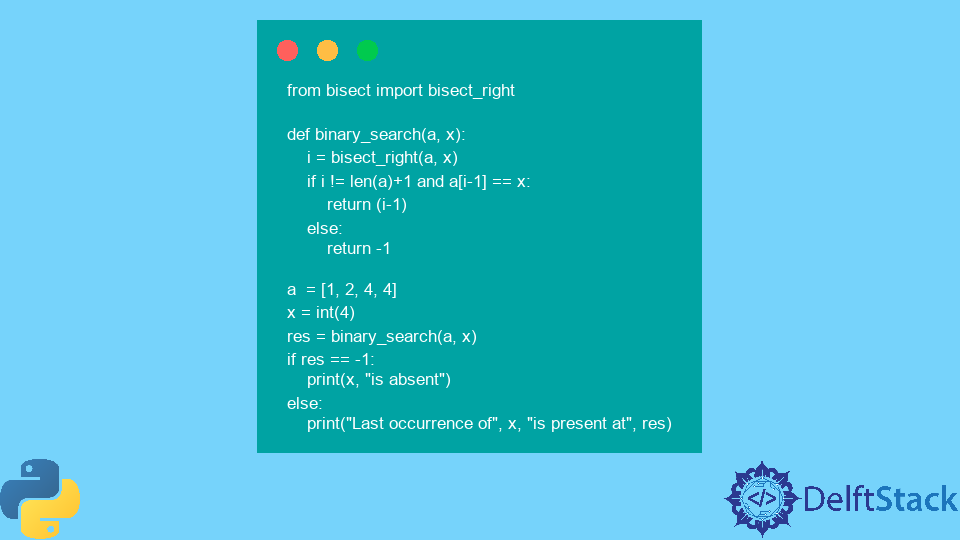
Find the last occurrence of an element
from bisect import bisect_right

def binary_search(a, x):
    i = bisect_right(a, x)
    if i != len(a)+1 and a[i-1] == x:
        return (i-1)
    else:
        return -1

a  = [1, 2, 4, 4]
x = int(4)
res = binary_search(a, x)
if res == -1:
    print(x, "is absent")
else:
    print("Last occurrence of", x, "is present at", res)
Output:
Last occurrence of 4 is present at 3
The purpose of Bisect algorithm is to find a position in list where an element needs to be inserted to keep the list sorted.
Python in its definition provides the bisect algorithms using the module “bisect” which allows keeping the list in sorted order after the insertion of each element. This is essential as this reduces overhead time required to sort the list again and again after the insertion of each element.
Important Bisection Functions
1. bisect(list, num, beg, end) :- This function returns the position in the sorted list, where the number passed in argument can be placed so as to maintain the resultant list in sorted order. If the element is already present in the list, the rightmost position where element has to be inserted is returned.
This function takes 4 arguments, list which has to be worked with, a number to insert, starting position in list to consider, ending position which has to be considered.
2. bisect_left(list, num, beg, end) :- This function returns the position in the sorted list, where the number passed in argument can be placed so as to maintain the resultant list in sorted order. If the element is already present in the list, the leftmost position where element has to be inserted is returned.
This function takes 4 arguments, list which has to be worked with, number to insert, starting position in list to consider, ending position which has to be considered.
3. bisect_right(list, num, beg, end) :- This function works similar to the “bisect()” and mentioned above.
Python3
import bisect
li = [1, 3, 4, 4, 4, 6, 7]
print ("Rightmost index to insert, so list remains sorted is : ",
end="")
print (bisect.bisect(li, 4))
print ("Leftmost index to insert, so list remains sorted is : ",
end="")
print (bisect.bisect_left(li, 4))
print ("Rightmost index to insert, so list remains sorted is : ",
end="")
print (bisect.bisect_right(li, 4, 0, 4))
Output
Rightmost index to insert, so list remains sorted is : 5
Leftmost index to insert, so list remains sorted is : 2
Rightmost index to insert, so list remains sorted is : 4
Time Complexity: O(log(n)), Bisect method works on the concept of binary search
Auxiliary Space: O(1)
4. insort(list, num, beg, end) :- This function returns the sorted list after inserting number in appropriate position, if the element is already present in the list, the element is inserted at the rightmost possible position.
This function takes 4 arguments, list which has to be worked with, number to insert, starting position in list to consider, ending position which has to be considered.
5. insort_left(list, num, beg, end) :- This function returns the sorted list after inserting number in appropriate position, if the element is already present in the list, the element is inserted at the leftmost possible position.
This function takes 4 arguments, list which has to be worked with, number to insert, starting position in list to consider, ending position which has to be considered.
6. insort_right(list, num, beg, end) :- This function works similar to the “insort()” as mentioned above.
Python3
import bisect
li1 = [1, 3, 4, 4, 4, 6, 7]
li2 = [1, 3, 4, 4, 4, 6, 7]
li3 = [1, 3, 4, 4, 4, 6, 7]
bisect.insort(li1, 5)
print ("The list after inserting new element using insort() is : ")
for i in range(0, 7):
print(li1[i], end=" ")
bisect.insort_left(li2, 5)
print("r")
print ("The list after inserting new element using insort_left() is : ")
for i in range(0, 7):
print(li2[i], end=" ")
print("r")
bisect.insort_right(li3, 5, 0, 4)
print ("The list after inserting new element using insort_right() is : ")
for i in range(0, 7):
print(li3[i], end=" ")
Output
The list after inserting new element using insort() is :
1 3 4 4 4 5 6
The list after inserting new element using insort_left() is :
1 3 4 4 4 5 6
The list after inserting new element using insort_right() is :
1 3 4 4 5 4 6
Time Complexity: O(n)
Auxiliary Space: O(1)