Использование функций потерь
Функция потерь (или объективная функция, или функция оценки результатов оптимизации) является одним из двух параметров, необходимых для компиляции модели:
model.compile(loss=’mean_squared_error’, optimizer=’sgd’)
from keras import losses
model.compile(loss=losses.mean_squared_error, optimizer=’sgd’)
Можно либо передать имя существующей функции потерь, либо передать символическую функцию TensorFlow/Theano, которая возвращает скаляр для каждой точки данных и принимает следующие два аргумента:
y_true: истинные метки. Тензор TensorFlow/Theano.
y_pred: Прогнозы. Тензор TensorFlow/Theano той же формы, что и y_true.
Фактически оптимизированная цель — это среднее значение выходного массива по всем точкам данных.
Доступные функции потери
mean_squared_error
keras.losses.mean_squared_error(y_true, y_pred)
mean_absolute_error
keras.losses.mean_absolute_error(y_true, y_pred)
mean_absolute_percentage_error
keras.losses.mean_absolute_percentage_error(y_true, y_pred)
mean_squared_logarithmic_error
keras.losses.mean_squared_logarithmic_error(y_true, y_pred)
squared_hinge
keras.losses.squared_hinge(y_true, y_pred)
hinge
keras.losses.hinge(y_true, y_pred)
categorical_hinge
keras.losses.categorical_hinge(y_true, y_pred)
logcosh
keras.losses.logcosh(y_true, y_pred)
Логарифм гиперболического косинуса ошибки прогнозирования.
log(cosh(x)) приблизительно равен (x ** 2) / 2 для малого x и abs(x) — log(2) для большого x. Это означает, что ‘logcosh’ работает в основном как средняя квадратичная ошибка, но не будет так сильно зависеть от случайного сильно неправильного предсказания.
Аргументы
- y_true: тензор истинных целей.
- y_pred: тензор прогнозируемых целей.
Возвращает
Тензор с одной записью о скалярной потере на каждый сэмпл.
huber_loss
keras.losses.huber_loss(y_true, y_pred, delta=1.0)
categorical_crossentropy
keras.losses.categorical_crossentropy(y_true, y_pred, from_logits=False, label_smoothing=0)
sparse_categorical_crossentropy
keras.losses.sparse_categorical_crossentropy(y_true, y_pred, from_logits=False, axis=-1)
binary_crossentropy
keras.losses.binary_crossentropy(y_true, y_pred, from_logits=False, label_smoothing=0)
kullback_leibler_divergence
keras.losses.kullback_leibler_divergence(y_true, y_pred)
poisson
keras.losses.poisson(y_true, y_pred)
cosine_proximity
keras.losses.cosine_proximity(y_true, y_pred, axis=-1)
is_categorical_crossentropy
keras.losses.is_categorical_crossentropy(loss)
Примечание: при использовании потери categorical_crossentropy ваши данные должны быть в категориальном формате (например, если у вас 10 классов, то целью для каждой выборки должен быть 10-мерный вектор, который является полностью нулевым, за исключением 1 в индексе, соответствующем классу выборки). Для того, чтобы преобразовать целые данные в категорические, можно использовать утилиту Keras to_categorical:
from keras.utils import to_categorical
categorical_labels = to_categorical(int_labels, num_classes=None)
При использовании переменной sparse_categorical_crossentropy loss, ваши данные должны быть целыми. Если у вас есть категориальные данные, следует использовать categoryical_crossentropy.
categoryical_crossentropy — это еще один термин для обозначения потери лога по нескольким классам.
You’ve created a deep learning model in Keras, you prepared the data and now you are wondering which loss you should choose for your problem.
We’ll get to that in a second but first what is a loss function?
In deep learning, the loss is computed to get the gradients with respect to model weights and update those weights accordingly via backpropagation. Loss is calculated and the network is updated after every iteration until model updates don’t bring any improvement in the desired evaluation metric.
So while you keep using the same evaluation metric like f1 score or AUC on the validation set during (long parts) of your machine learning project, the loss can be changed, adjusted and modified to get the best evaluation metric performance.
You can think of the loss function just like you think about the model architecture or the optimizer and it is important to put some thought into choosing it. In this piece we’ll look at:
- loss functions available in Keras and how to use them,
- how you can define your own custom loss function in Keras,
- how to add sample weighing to create observation-sensitive losses,
- how to avoid nans in the loss,
- how you can monitor the loss function via plotting and callbacks.
Let’s get into it!
Keras loss functions 101
In Keras, loss functions are passed during the compile stage, as shown below.
In this example, we’re defining the loss function by creating an instance of the loss class. Using the class is advantageous because you can pass some additional parameters.
from tensorflow import keras
from tensorflow.keras import layers

model = keras.Sequential()
model.add(layers.Dense(64, kernel_initializer='uniform', input_shape=(10,)))
model.add(layers.Activation('softmax'))

loss_function = keras.losses.SparseCategoricalCrossentropy(from_logits=True)
model.compile(loss=loss_function, optimizer='adam')
If you want to use a loss function that is built into Keras without specifying any parameters you can just use the string alias as shown below:
model.compile(loss='sparse_categorical_crossentropy', optimizer='adam')
You might be wondering how does one decide on which loss function to use?
There are various loss functions available in Keras. Other times you might have to implement your own custom loss functions.
Let’s dive into all those scenarios.
Which loss functions are available in Keras?
Binary Classification
Binary classification loss function comes into play when solving a problem involving just two classes. For example, when predicting fraud in credit card transactions, a transaction is either fraudulent or not.
Binary Cross Entropy
The Binary Cross entropy will calculate the cross-entropy loss between the predicted classes and the true classes. By default, the sum_over_batch_size reduction is used. This means that the loss will return the average of the per-sample losses in the batch.
y_true = [[0., 1.], [0.2, 0.8],[0.3, 0.7],[0.4, 0.6]]
y_pred = [[0.6, 0.4], [0.4, 0.6],[0.6, 0.4],[0.8, 0.2]]
bce = tf.keras.losses.BinaryCrossentropy(reduction='sum_over_batch_size')
bce(y_true, y_pred).numpy()
The sum reduction means that the loss function will return the sum of the per-sample losses in the batch.
bce = tf.keras.losses.BinaryCrossentropy(reduction='sum')
bce(y_true, y_pred).numpy()
Using the reduction as none returns the full array of the per-sample losses.
bce = tf.keras.losses.BinaryCrossentropy(reduction='none')
bce(y_true, y_pred).numpy()
array([0.9162905 , 0.5919184 , 0.79465103, 1.0549198 ], dtype=float32)
In binary classification, the activation function used is the sigmoid activation function. It constrains the output to a number between 0 and 1.
Multiclass classification
Problems involving the prediction of more than one class use different loss functions. In this section we’ll look at a couple:
Categorical Crossentropy
The CategoricalCrossentropy also computes the cross-entropy loss between the true classes and predicted classes. The labels are given in an one_hot format.
cce = tf.keras.losses.CategoricalCrossentropy()
cce(y_true, y_pred).numpy()
Sparse Categorical Crossentropy
If you have two or more classes and the labels are integers, the SparseCategoricalCrossentropy should be used.
y_true = [0, 1,2]
y_pred = [[0.05, 0.95, 0], [0.1, 0.8, 0.1],[0.1, 0.8, 0.1]]
scce = tf.keras.losses.SparseCategoricalCrossentropy()
scce(y_true, y_pred).numpy()
The Poison Loss
You can also use the Poisson class to compute the poison loss. It’s a great choice if your dataset comes from a Poisson distribution for example the number of calls a call center receives per hour.
y_true = [[0.1, 1.,0.8], [0.1, 0.9,0.1],[0.2, 0.7,0.1],[0.3, 0.1,0.6]]
y_pred = [[0.6, 0.2,0.2], [0.2, 0.6,0.2],[0.7, 0.1,0.2],[0.8, 0.1,0.1]]
p = tf.keras.losses.Poisson()
p(y_true, y_pred).numpy()
Kullback-Leibler Divergence Loss
The relative entropy can be computed using the KLDivergence class. According to the official docs at PyTorch:
KL divergence is a useful distance measure for continuous distributions and is often useful when performing direct regression over the space of (discretely sampled) continuous output distributions.
y_true = [[0.1, 1.,0.8], [0.1, 0.9,0.1],[0.2, 0.7,0.1],[0.3, 0.1,0.6]]
y_pred = [[0.6, 0.2,0.2], [0.2, 0.6,0.2],[0.7, 0.1,0.2],[0.8, 0.1,0.1]]
kl = tf.keras.losses.KLDivergence()
kl(y_true, y_pred).numpy()
In a multi-class problem, the activation function used is the softmax function.
Object Detection
The Focal Loss
In classification problems involving imbalanced data and object detection problems, you can use the Focal Loss. The loss introduces an adjustment to the cross-entropy criterion.
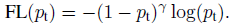
It is done by altering its shape in a way that the loss allocated to well-classified examples is down-weighted. This ensures that the model is able to learn equally from minority and majority classes.
The cross-entropy loss is scaled by scaling the factors decaying at zero as the confidence in the correct class increases. The factor of scaling down weights the contribution of unchallenging samples at training time and focuses on the challenging ones.
import tensorflow_addons as tfa

y_true = [[0.97], [0.91], [0.03]]
y_pred = [[1.0], [1.0], [0.0]]
sfc = tfa.losses.SigmoidFocalCrossEntropy()
sfc(y_true, y_pred).numpy()
array([0.00010971, 0.00329749, 0.00030611], dtype=float32)
Generalized Intersection over Union
The Generalized Intersection over Union loss from the TensorFlow add on can also be used. The Intersection over Union (IoU) is a very common metric in object detection problems. IoU is however not very efficient in problems involving non-overlapping bounding boxes.
The Generalized Intersection over Union was introduced to address this challenge that IoU is facing. It ensures that generalization is achieved by maintaining the scale-invariant property of IoU, encoding the shape properties of the compared objects into the region property, and making sure that there is a strong correlation with IoU in the event of overlapping objects.
gl = tfa.losses.GIoULoss()
boxes1 = tf.constant([[4.0, 3.0, 7.0, 5.0], [5.0, 6.0, 10.0, 7.0]])
boxes2 = tf.constant([[3.0, 4.0, 6.0, 8.0], [14.0, 14.0, 15.0, 15.0]])
loss = gl(boxes1, boxes2)
Regression
In regression problems, you have to calculate the differences between the predicted values and the true values but as always there are many ways to do it.
Mean Squared Error
The MeanSquaredError class can be used to compute the mean square of errors between the predictions and the true values.
y_true = [12, 20, 29., 60.]
y_pred = [14., 18., 27., 55.]
mse = tf.keras.losses.MeanSquaredError()
mse(y_true, y_pred).numpy()
Use Mean Squared Error when you desire to have large errors penalized more than smaller ones.
Mean Absolute Percentage Error
The mean absolute percentage error is computed using the function below.

It is calculated as shown below.
y_true = [12, 20, 29., 60.]
y_pred = [14., 18., 27., 55.]
mape = tf.keras.losses.MeanAbsolutePercentageError()
mape(y_true, y_pred).numpy()
Consider using this loss when you want a loss that you can explain intuitively. People understand percentages easily. The loss is also robust to outliers.
Mean Squared Logarithmic Error
The mean squared logarithmic error can be computed using the formula below:
Here’s an implementation of the same:
y_true = [12, 20, 29., 60.]
y_pred = [14., 18., 27., 55.]
msle = tf.keras.losses.MeanSquaredLogarithmicError()
msle(y_true, y_pred).numpy()
Mean Squared Logarithmic Error penalizes underestimates more than it does overestimates. It’s a great choice when you prefer not to penalize large errors, it is, therefore, robust to outliers.
Cosine Similarity Loss
If your interest is in computing the cosine similarity between the true and predicted values, you’d use the CosineSimilarity class. It is computed as:
The result is a number between -1 and 1 . 0 indicates orthogonality while values close to -1 show that there is great similarity.
y_true = [[12, 20], [29., 60.]]
y_pred = [[14., 18.], [27., 55.]]
cosine_loss = tf.keras.losses.CosineSimilarity(axis=1)
cosine_loss(y_true, y_pred).numpy()
LogCosh Loss
The LogCosh class computes the logarithm of the hyperbolic cosine of the prediction error.
Here’s its implementation as a stand-alone function.
y_true = [[12, 20], [29., 60.]]
y_pred = [[14., 18.], [27., 55.]]
l = tf.keras.losses.LogCosh()
l(y_true, y_pred).numpy()
LogCosh Loss works like the mean squared error, but will not be so strongly affected by the occasional wildly incorrect prediction. — TensorFlow Docs
Huber loss
For regression problems that are less sensitive to outliers, the Huber loss is used.
y_true = [12, 20, 29., 60.]
y_pred = [14., 18., 27., 55.]
h = tf.keras.losses.Huber()
h(y_true, y_pred).numpy()
Learning Embeddings
Triplet Loss
You can also compute the triplet loss with semi-hard negative mining via TensorFlow addons. The loss encourages the positive distances between pairs of embeddings with the same labels to be less than the minimum negative distance.
import tensorflow_addons as tfa

model.compile(optimizer='adam',
              loss=tfa.losses.TripletSemiHardLoss(),
              metrics=['accuracy'])
Creating custom loss functions in Keras
Sometimes there is no good loss available or you need to implement some modifications. Let’s learn how to do that.
A custom loss function can be created by defining a function that takes the true values and predicted values as required parameters. The function should return an array of losses. The function can then be passed at the compile stage.
def custom_loss_function(y_true, y_pred):
   squared_difference = tf.square(y_true - y_pred)
   return tf.reduce_mean(squared_difference, axis=-1)

model.compile(optimizer='adam', loss=custom_loss_function)
Let’s see how we can apply this custom loss function to an array of predicted and true values.
import numpy as np

y_true = [12, 20, 29., 60.]
y_pred = [14., 18., 27., 55.]
cl = custom_loss_function(np.array(y_true),np.array(y_pred))
cl.numpy()
Use of Keras loss weights
During the training process, one can weigh the loss function by observations or samples. The weights can be arbitrary, but a typical choice is class weights (distribution of labels). Each observation is weighted by the fraction of the class it belongs to (reversed) so that the loss for minority class observations is more important when calculating the loss.
One of the ways to do this is to pass the class weights during the training process.
The weights are passed using a dictionary that contains the weight for each class. You can compute the weights using Scikit-learn or calculate the weights based on your own criterion.
weights = { 0:1.01300017,1:0.88994364,2:1.00704935, 3:0.97863318,      4:1.02704553, 5:1.10680686,6:1.01385603,7:0.95770152, 8:1.02546573,
               9:1.00857287}
model.fit(x_train, y_train,verbose=1, epochs=10,class_weight=weights)
The second way is to pass these weights at the compile stage.
weights = [1.013, 0.889, 1.007, 0.978, 1.027,1.106,1.013,0.957,1.025, 1.008]

model.compile(optimizer=tf.keras.optimizers.SGD(),
              loss=tf.keras.losses.SparseCategoricalCrossentropy(),
              loss_weights=weights,
              metrics=['accuracy'])
How to monitor Keras loss function [example]
It is usually a good idea to monitor the loss function on the training and validation set as the model is training. Looking at those learning curves is a good indication of overfitting or other problems with model training.
There are two main options of how this can be done.
Monitor Keras loss using console logs
The quickest and easiest way to log and look at the losses is simply printing them to the console.
import tensorflow as tf

mnist = tf.keras.datasets.mnist
(x_train, y_train), (x_test, y_test) = mnist.load_data()
x_train, x_test = x_train / 255.0, x_test / 255.0

model = tf.keras.models.Sequential([
   tf.keras.layers.Flatten(input_shape=(28, 28)),
   tf.keras.layers.Dense(512, activation='relu'),
   tf.keras.layers.Dropout(0.2),
   tf.keras.layers.Dense(10, activation='softmax')
])

model.compile(optimizer='sgd',
             loss='sparse_categorical_crossentropy',
             metrics=['accuracy'])

model.fit(x_train, y_train,verbose=1, epochs=10)
The problem with this approach is that those logs can be easily lost, it is difficult to see progress, and when working on remote machines, you may not have access to it.
Monitor Keras loss using a callback
Another cleaner option is to use a callback that will log the loss somewhere on every batch and epoch ended.
You need to decide where and what you would like to log, but it is really simple.
For example, logging Keras loss to neptune.ai could look like this:
from keras.callbacks import Callback

class NeptuneCallback(Callback):
    def on_batch_end(self, batch, logs=None):
        for metric_name, metric_value in logs.items():
            neptune_run[f"{metric_name}"].log(metric_value)

    def on_epoch_end(self, epoch, logs=None):
        for metric_name, metric_value in logs.items():
            neptune_run[f"{metric_name}"].log(metric_value)
You can create the monitoring callback yourself or use one of the many available Keras callbacks both in the Keras library and in other libraries that integrate with it, like neptune.ai, TensorBoard, and others.
Once you have the callback ready, you simply pass it to the model.fit(...):
pip install neptune-tensorflow-keras# the same as above
import neptune.new as neptune
from neptune.new.integrations.tensorflow_keras import NeptuneCallback
run = neptune.init_run()
neptune_callback = NeptuneCallback(run=run)
model.fit(
x_train,
y_train,
validation_split=0.2,
epochs=10,
callbacks=[neptune_callback],
)
And monitor your experiment learning curves in the web app:
Note: For the most up-to-date code examples, please refer to the Neptune-Keras integration docs.
With neptune.ai, you can not only track losses, but also other metrics and parameters, as well as artifacts, source code, system metrics and more.
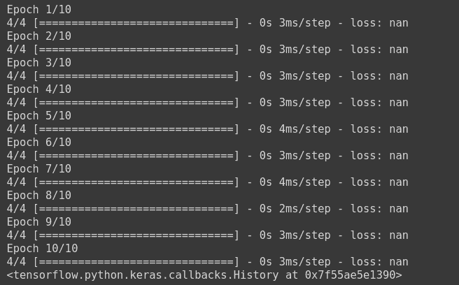
Why Keras loss nan happens
Most of the time, losses you log will be just some regular values, but sometimes you might get nans when working with Keras loss functions.

When that happens, your model will not update its weights and will stop learning, so this situation needs to be avoided.
There could be many reasons for nan loss but usually, what happens is:
- nans in the training set will lead to nans in the loss,
- NumPy infinite in the training set will also lead to nans in the loss,
- Using a training set that is not scaled,
- Use of very large l2 regularizers and a learning rate above 1,
- Use of the wrong optimizer function,
- Large (exploding) gradients that result in a large update to network weights during training.
So in order to avoid nans in the loss, ensure that:
- Check that your training data is properly scaled and doesn’t contain nans;
- Check that you are using the right optimizer and that your learning rate is not too large;
- Check whether the l2 regularization is not too large;
- If you are facing the exploding gradient problem, you can either: re-design the network or use gradient clipping so that your gradients have a certain “maximum allowed model update”.
Vanishing and Exploding Gradients in Neural Network Models: Debugging, Monitoring, and Fixing
Understanding Gradient Clipping (and How It Can Fix Exploding Gradients Problem)
Final thoughts
Hopefully, this article gave you some background into loss functions in Keras.
We’ve covered:
- Built-in loss functions in Keras,
- Implementation of your own custom loss functions,
- How to add sample weighing to create observation-sensitive losses,
- How to avoid loss nans,
- How you can visualize loss as your model is training.
For more information, check out the Keras Repository and the TensorFlow Loss Functions documentation.

In this article, there is an in-depth discussion on
- What are Loss Functions
- What are Evaluation Metrics?
- Commonly used Loss functions in Keras (Regression and Classification)
- Built-in loss functions in Keras
- What is the custom loss function?
- Implementation of common loss functions in Keras
- Custom Loss Function for Layers i.e Custom Regularization Loss
- Dealing with NaN values in Keras Loss
- Why should you use a Custom Loss?
- Monitoring Keras Loss using callbacks
What are Loss Functions
Loss functions are one of the core parts of a machine learning model. If you’ve been in the field of data science for some time, you must have heard it. Loss functions, also known as cost functions, are special types of functions, which help us minimize the error, and reach as close as possible to the expected output.
In deep learning, the loss is computed to get the gradients for the model weights and update those weights accordingly using backpropagation.
Basic working or understanding of error can be gained from the image above, where there is an actual value and a predicted value. The difference between the actual value and predicted value can be known as error.
This can be written in the equation form as

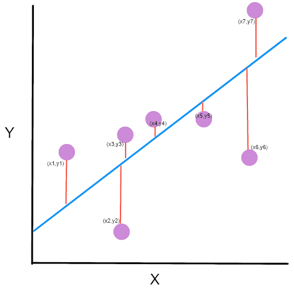
So our goal is to minimize the difference between the predicted value which is hθ(x) and the actual value y. In other words, you have to minimize the value of the cost function. This main idea can be understood better from the following picture by Professor Andrew NG where he explains that choosing the correct value of θ0 and θ1 which are weights of a model, such that our prediction hθ is closest to y which is the actual output.
Here Professor Andrew NG is using the Mean Squared Error function, which will be discussed later on.
An easy explanation can be said that the goal of a machine learning model is to minimize the cost and maximize the evaluation metric. This can be achieved by updating the weights of a machine learning model using some algorithm such as Gradient Descent.
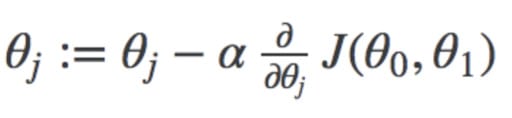
Here you can see the weight that is being updated and the cost function, that is used to update the weight of a machine learning model.
What are Evaluation Metrics
Evaluation metrics are the metrics used to evaluate and judge the performance of a machine learning model. Evaluating a machine learning project is very essential. There are different types of evaluation metrics such as ‘Mean Squared Error’, ‘Accuracy’, ‘Mean Absolute Error’ etc. The cost functions used, such as mean squared error, or binary cross-entropy are also metrics, but they are difficult to read and interpret how our model is performing. So there is a need for other metrics like Accuracy, Precision, Recall, etc. Using different metrics is important because a model may perform well using one measurement from one evaluation metric, but may perform poorly using another measurement from another evaluation metric.
![]()
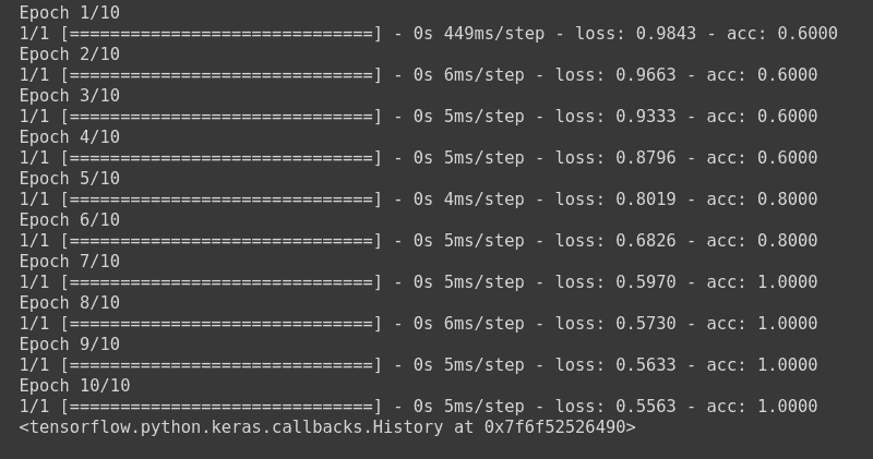
Here you can see the performance of our model using 2 metrics. The first one is Loss and the second one is accuracy. It can be seen that our loss function (which was cross-entropy in this example) has a value of 0.4474 which is difficult to interpret whether it is a good loss or not, but it can be seen from the accuracy that currently it has an accuracy of 80%.
Hence it is important to use different evaluation metrics other than loss/cost function only to properly evaluate the model’s performance and capabilities.
Some of the common evaluation metrics include:
- Accuracy
- Precision
- Recall
- F-1 Score
- MSE
- MAE
- Confusion Matrix
- Logarithmic Loss
- ROC curve
And many more.
Commonly Used Loss Functions in Machine Learning Algorithms and their Keras Implementation
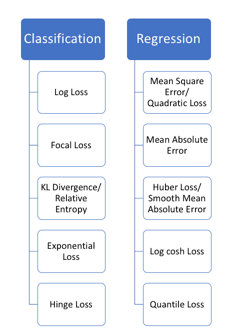
Common Regression Losses:
Regression is the type of problem where you are going to predict a continuous variable. This means that our variable can be any number, not some specific labels.
For example, when you have to predict prices of houses, it can be a house of any price, so it is a regression problem.
Some of the common examples of regressions tasks are
- Prices Prediction
- Stock Market Prediction
- Financial Forecasting
- Trend Analysis
- Time Series Predictions
And many more.
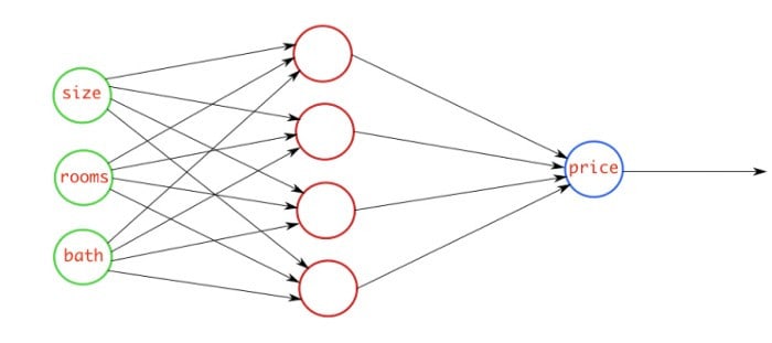
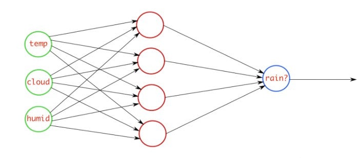
This figure above explains the regression problem where you are going to predict the price of the house by checking three features which are size of the house, rooms in the house, and baths in the house. Our model will check these features, and will predict a continuous number that will be the price of the house.
Since regression problems deal with predicting a continuous number, so you have to use different types of loss then classification problems. Some of the commonly used loss functions in regression problems are as follows.
Mean Squared Error
Mean squared error, also known as L2 Loss is mainly used for Regression Tasks. As the name suggests, it is calculated by taking the mean of the square of the loss/error which is the difference between actual and predicted value.
The Mathematical equation for Mean Squared Error is
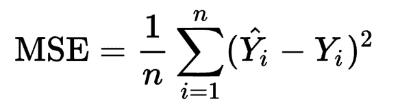
Where Ŷi is the predicted value, and Yi is the actual value. Mean Squared Error penalizes the model for making errors by taking the square. This is the reason that this loss function is less robust to outliers in the dataset.
Implementation in Keras.
					import keras
import numpy as np

y_true = np.array([[10.0,7.0]]) #sample data
y_pred = np.array([[8.0, 6.0]])

a = keras.losses.MSE(y_true, y_pred)

print(f'Value of Mean Squared Error is {a.numpy()}')
![]()
Here predicted values and the true values are passed inside the Mean Squared Error Object from keras.losses and computed the loss. It returns a tf.Tensor object which has been converted into numpy to see more clearly.
Using via compile Method:
Keras losses can be specified for a deep learning model using the compile method from keras.Model..
					model = keras.Sequential([
                     keras.layers.Dense(10, input_shape=(1,), activation='relu'),
                     keras.layers.Dense(1)

])
And now the compile method can be used to specify the loss and metrics.
model.compile(loss='mse', optimizer='adam')
Now when our model is going to be trained, it will use the Mean Squared Error loss function to compute the loss, update the weights using ADAM optimizer.
model.fit(np.array([[10.0],[20.0], [30.0],[40.0],[50.0],[60.0],[10.0], [20.0]]), np.array([6, 12, 18,24,30, 36,6, 12]), epochs=10)
Mean Absolute Error
Mean Absolute error, also known as L1 Error, is defined as the average of the absolute differences between the actual value and the predicted value. This is the average of the absolute difference between the predicted and the actual value.
Mathematically, it can be shown as:
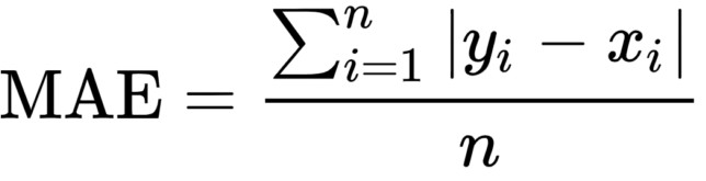
The Mean Absolute error uses the scale-dependent accuracy measure which means that it uses the same scale which is being used by the data being measured, thus it can not be used in making comparisons between series that are using different scales.
Mean Squared Error is also a common regression loss, which means that it is used to predict a continuous variable.
Standalone Implementation in Keras:
					import keras
import numpy as np


y_true = np.array([[10.0,7.0]]) #dummy data
y_pred = np.array([[8.0, 6.0]])

c = keras.losses.MAE(y_true, y_pred) #calculating loss

print(f'Value of Mean Absolute Error is {c.numpy()}')
![]()
What you have to do is to create an MAE object from keras.losses and pass in our true and predicted labels to calculate the loss using the equation given above.
Implementing using compile method
When working with a deep learning model in Keras, you have to define the model structure first.
					model = keras.models.Sequential([
                                   keras.layers.Dense(10, input_shape=(1,), activation='relu'),
                                   keras.layers.Dense(1)
])
After defining the model architecture, you have to compile it and use the MAE loss function. Notice that either there is linear or no activation function in the last layer means that you are going to predict a continuous variable.
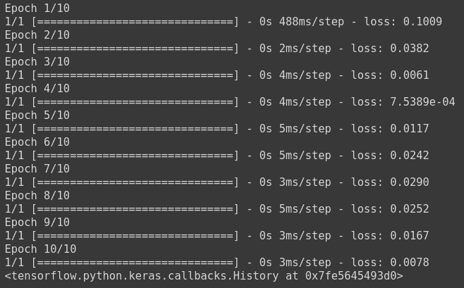
model.compile(loss='mae', optimizer='adam')
You can now simply just fit the model to check our model’s progress. Here our model is going to train on a very small dummy random array just to check the progress.
model.fit(np.array([[10.0],[20.0], [30.0],[40.0],[50.0],[60.0],[10.0], [20.0]]), np.array([6, 12, 18,24,30, 36,6, 12]), epochs=10)
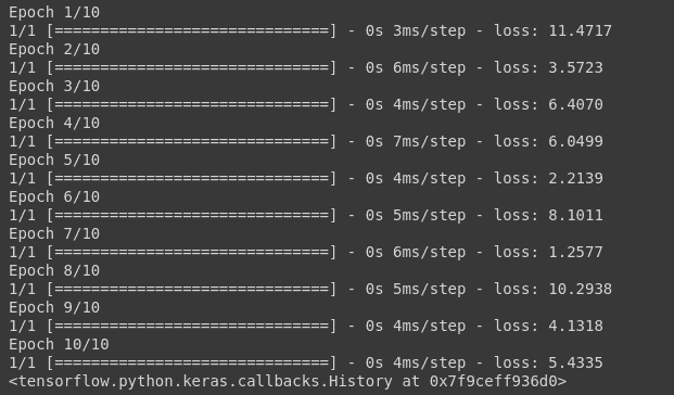
And you can see the loss value which has been calculated using the MAE formula for each epoch.
Common Classification Losses:
Classification problems are those problems, in which you have to predict a label. This means that the output should be only from the given labels that you have provided to the model.
For example: There is a problem where you have to detect if the input image belongs to any given class such as dog, cat, or horse. The model will predict 3 numbers ranging from 0 to 1 and the one with the highest probability will be picked
If you want to predict whether it is going to rain tomorrow or not, this means that the model can output between 0 and 1, and you will choose the option of rain if it is greater than 0.5, and no rain if it is less than 0.5.
Common Classification Loss:
1. Cross-Entropy
Cross Entropy is one of the most commonly used classification loss functions. You can say that it is the measure of the degrees of the dissimilarity between two probabilistic distributions. For example, in the task of predicting whether it will rain tomorrow or not, there are two distributions, one for True, and one for False.
Cross Entropy is of 3 main types.
a. Binary Cross Entropy
Binary Cross Entropy, as the name suggests, is the cross entropy that occurs between two classes, or in the problem of binary classification where you have to detect whether it belongs to class ‘A’, and if it does not belong to class ‘A’, then it belongs to class ‘B’.
Just like in the example of rain prediction, if it is going to rain tomorrow, then it belongs to rain class, and if there is less probability of rain tomorrow, then this means that it belongs to no rain class.
Mathematical Equation for Binary Cross Entropy is

This loss function has 2 parts. If our actual label is 1, the equation after ‘+’ becomes 0 because 1-1 = 0. So loss when our label is 1 is
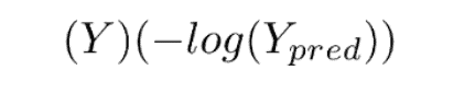
And when our label is 0, then the first part becomes 0. So our loss in that case would be
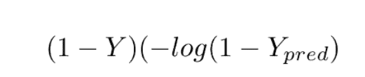
This loss function is also known as the Log Loss function, because of the logarithm of the loss.
Standalone Implementation:
You can create an object for Binary Cross Entropy from Keras.losses. Then you have to pass in our true and predicted labels.
					import keras
import numpy as np

y_true=np.array([[1.0]])
y_pred = np.array([[0.9]])

loss = keras.losses.BinaryCrossentropy()
print(f"BCE LOSS VALUE IS {loss(y_true, y_pred).numpy()}")
![]()
Implementation using compile method
To use Binary Cross Entropy in a deep learning model, design the architecture, and compile the model while specifying the loss as Binary Cross Entropy.
					import keras
import numpy as np

model = keras.models.Sequential([
                                   keras.layers.Dense(16, input_shape=(2,), activation='relu'),
                                   keras.layers.Dense(8, activation='relu'),
                                   keras.layers.Dense(1, activation='sigmoid') #Sigmoid for probabilistic distribution
])
model.compile(optimizer='sgd', loss=keras.losses.BinaryCrossentropy(), metrics=['acc'])# binary cross entropy

model.fit(np.array([[10.0, 20.0],[20.0,30.0],[30.0,6.0], [8.0, 20.0]]),np.array([1,1,0,1]) ,epochs=10)
This will train the model using Binary Cross Entropy Loss function.
b. Categorical Cross Entropy
Categorical Cross Entropy is the cross entropy that is used for multi-class classification. This means for a single training example, you have n probabilities, and you take the class with maximum probability where n is number of classes.

Mathematically, you can write it as:

This double sum is over the N number of examples and C categories. The term 1yi ∈ Cc shows that the ith observation belongs to the cth category. The Pmodel[yi ∈ Cc] is the probability predicted by the model for the ith observation to belong to the cth category. When there are more than 2 probabilities, the neural network outputs a vector of C probabilities, with each probability belonging to each class. When the number of categories is just two, the neural network outputs a single probability ŷi , with the other one being 1 minus the output. This is why the binary cross entropy looks a bit different from categorical cross entropy, despite being a special case of it.
Standalone Implementation
You will create a Categorical Cross Entropy object from keras.losses and pass in our true and predicted labels, on which it will calculate the Cross Entropy and return a Tensor.
Note that you have to provide a matrix that is one hot encoded showing probability for each class, as shown in this example.
					import keras
import numpy as np

y_true = [[0, 1, 0], [0, 0, 1]] #3classes

y_pred = [[0.05, 0.95, 0], [0.1, 0.5, 0.4]]


loss = keras.losses.CategoricalCrossentropy()
print(f"CCE LOSS VALUE IS {loss(y_true, y_pred).numpy()}")
![]()
Implementation using compile method
When implemented using the compile method, you have to design a model in Keras, and compile it using Categorical Cross Entropy loss. Now when the model is trained, it is calculating the loss based on categorical cross entropy, and updating the weights according to the given optimizer.
					import keras
import numpy as np
from keras.utils import to_categorical #to one hot encode the data

model = keras.models.Sequential([
                                   keras.layers.Dense(16, input_shape=(2,), activation='relu'),
                                   keras.layers.Dense(8, activation='relu'),
                                   keras.layers.Dense(3, activation='softmax') #Softmax for multiclass probability
])

model.compile(optimizer='sgd', loss=keras.losses.CategoricalCrossentropy(), metrics=['acc'])# categorical cross entropy

model.fit(np.array([[10.0, 20.0],[20.0,30.0],[30.0,6.0], [8.0, 20.0], [-1.0, -100.0], [-10.0, -200.0]]) ,to_categorical(np.array([1,1,0,1, 2, 2])) ,epochs=10)
Here, it will train the model on our dummy dataset.
c. Sparse Categorical Cross Entropy
Mathematically, there is no difference between Categorical Cross Entropy, and Sparse Categorical Cross Entropy according to official documentation. Use this cross entropy loss function when there are two or more label classes. We expect labels to be provided as integers. If you want to provide labels using one-hot representation, please use CategoricalCrossentrop loss. There should be # classes floating point values per feature for y_pred and a single floating point value per feature for y_true.“
As you have seen earlier in Categorical Cross Entropy that one hot matrix has been passed as the true labels, and predicted labels. An example of which is as follows:
to_categorical(np.array([1,1,0,1, 2, 2]))
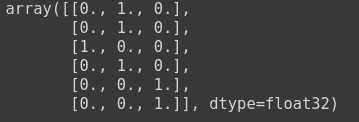
For using sparse categorical cross entropy in Keras, you need to pass in the label encoded labels. You can use sklearn for this purpose.
Lets see this example to understand better.
					from sklearn.preprocessing import LabelEncoder

le = LabelEncoder()
output = le.fit_transform(np.array(['High chance of Rain', 'No Rain', 'Maybe', 'Maybe', 'No Rain', 'High chance of Rain']))
Here a LabelEncoder object has been created, and the fit_transform method is used to encode it. The output of it is as follows.
![]()
Standalone Implementation
To perform standalone implementation, you need to perform label encoding on labels. There should be n floating point values per feature for each true label, where n is the total number of classes.
					from sklearn.preprocessing import LabelEncoder
t = LabelEncoder()
y_pred = [[0.1,0.1,0.8], [0.1,0.4,0.5], [0.5,0.3,0.2], [0.6,0.3,0.1]]
y_true = t.fit_transform(['Rain', 'Rain', 'High Changes of Rain', 'No Rain'])
loss = keras.losses.SparseCategoricalCrossentropy()
print(f"Sparse Categorical Loss is {loss(y_true, y_pred).numpy()} ")
![]()
Implementation using model.compile
To implement Sparse Categorical Cross Entropy in a deep learning model, you have to design the model, and compile it using the loss sparse categorical cross entropy. Remember to perform label encoding of your class labels so that sparse categorical cross entropy can work.
					import keras
import numpy as np
from sklearn.preprocessing import LabelEncoder
model = keras.models.Sequential([
                                   keras.layers.Dense(16, input_shape=(2,), activation='relu'),
                                   keras.layers.Dense(8, activation='relu'),
                                   keras.layers.Dense(3, activation='softmax') #Softmax for multiclass probability
])
le = LabelEncoder()
model.compile(optimizer='sgd', loss=keras.losses.SparseCategoricalCrossentropy(), metrics=['acc'])# sparse categorical cross entropy
Now the model will be trained on the dummy dataset.
model.fit(np.array([[10.0, 20.0],[20.0,30.0],[30.0,6.0], [8.0, 20.0], [-1.0, -100.0], [-10.0, -200.0]]) ,le.fit_transform(np.array(['High chance of Rain', 'High chance of Rain', 'High chance of Rain', 'Maybe', 'No Rain', 'No Rain'])) ,epochs=10)
The model has been trained, where the loss is calculated using sparse categorical cross entropy, and the weights have been updated using stochastic gradient descent.
2. Hinge Loss
Hinge loss is a commonly used loss function for classification problems. It is mainly used in problems where you have to do ‘maximum-margin’ classification. A common example of which is Support Vector Machines.
The following image shows how maximum margin classification works.
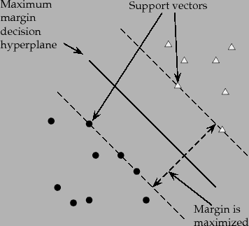
Source: Stanford NLP Group
The mathematical formula for hinge loss is:
Where yi is the actual label and ŷ is the predicted label. When prediction is positive, value goes on one side, and when the prediction is negative, value goes totally opposite. This is why it is known as maximum margin classification.
Standalone Implementation:
To perform standalone implementation of Hinge Loss in Keras, you are going to use Hinge Loss Class from keras.losses.
					import keras
import numpy as np
y_true = [[0., 1.], [0., 0.]]
y_pred = [[0.6, 0.4], [0.4, 0.6]]
h = keras.losses.Hinge()
print(f'Value for Hinge Loss is {h(y_true, y_pred).numpy()}')
![]()
Implementation using compile Method
To implement Hinge loss using compile method, you will design our model and compile it where you will mention our loss as Hinge.
Note that Hinge Loss works best with tanh as the activation in the last layer.
					import keras
import numpy as np
					model = keras.models.Sequential([
                                   keras.layers.Dense(16, input_shape=(2,), activation='relu'),
                                   keras.layers.Dense(8, activation='tanh'),
                                   keras.layers.Dense(1, activation='tanh')
])
model.compile(optimizer='adam', loss=keras.losses.Hinge(), metrics=['acc'])# Hinge Loss
					from sklearn.preprocessing import LabelEncoder

le = LabelEncoder()
model.fit(np.array([[10.0, 20.0],[20.0,30.0],[30.0,6.0], [-1.0, -100.0], [-10.0, -200.0]]) ,le.fit_transform(np.array(['High chance of Rain', 'High chance of Rain', 'High chance of Rain', 'No Rain', 'No Rain'])) ,epochs=10, batch_size=5)
This will train the model using Hinge Loss and update the weights using Adam optimizer.
Custom Loss Functions
So far you have seen some of the important cost functions that are widely used in industry and are good and easy to understand, and are built-in by famous deep learning frameworks such as Keras, or PyTorch. These built-in loss functions are enough for most of the typical tasks such as classification, or regression.
But there are some tasks, which can not be performed well using these built-in loss functions, and require some other loss that is more suitable for that task. For that purpose, a custom loss function is designed that calculates the error between the predicted value and actual value based on custom criteria.
Why you should use Custom Loss
Artificial Intelligence in general and Deep Learning in general is a very strong research field. There are various industries using Deep Learning to solve complex scenarios.
There is a lot of research on how to perform a specific task using Deep Learning. For example there is a task on generating different recipes of food using the picture of the food. Now on papers with code (a famous site for deep learning and machine learning research papers), there are a lot of research papers on this topic.

Now Imagine you are reading a research paper where the researchers thought that using Cross Entropy, or Mean Squared Error, or whatever the general loss function is for that specific type of the problem is not good enough. It may require you to modify it according to the need. This may involve adding some new parameters, or a whole new technique to achieve better results.
Now when you are implementing that problem, or you hired some data scientists to solve that specific problem for you, you may find that this specific problem is best solved using that specific loss function which is not available by default in Keras, and you need to implement it yourself.
A custom loss function can improve the models performance significantly, and can be really useful in solving some specific problems.
To create a custom loss, you have to take care of some rules.
- The loss function must only take two values, that are true labels, and predicted labels. This is because in order to calculate the error in prediction, these two values are needed. These arguments are passed from the model itself when the model is being fitted.
For example:
					def customLoss(y_true, y_pred):
            	return loss
	model.compile(loss=customLoss, optimizer='sgd')
2. Make sure that you are making the use of y_pred or predicted value in the loss function, because if you do not do so, the gradient expression would not be defined, and it can throw some error.
3. You can now simply use it in model.compile function just like you would use any other loss function.
Example:
Let’s say you want to perform a regression task where you want to use a custom loss function that divides the loss value of Mean Squared Error by 10. Mathematically, it can be denoted as:
Now to implement it in Keras, you need to define a custom loss function, with two parameters that are true and predicted values. Then you will perform mathematical functions as per our algorithm, and return the loss value.
Note that Keras Backend functions and Tensorflow mathematical operations will be used instead of numpy functions to avoid some silly errors. Keras backend functions work similarly to numpy functions.
					import keras
import numpy as np
from tensorflow.python.ops import math_ops

def custom_loss(y_true, y_pred):
 diff = math_ops.squared_difference(y_pred, y_true)  #squared difference
 loss = K.mean(diff, axis=-1) #mean over last dimension
 loss = loss / 10.0
 return loss
Here you can see a custom function with 2 parameters that are true and predicted values, and the first step was to calculate the squared difference between the predicted labels and the true labels using squared difference function from Tensorflow Python ops. Then the mean is calculated to complete the mean squared error, and divided by 10 to complete our algorithm. The loss value is then returned.
You can use it in our deep learning model, by compiling our model and setting the loss function to the custom loss defined above.
					model = keras.Sequential([
                   keras.layers.Dense(10, activation='relu', input_shape=(1,)),
                   keras.layers.Dense(1)
])

model.compile(loss=custom_loss, optimizer='sgd')

X_train = np.array([[10.0],[20.0], [30.0],[40.0],[50.0],[60.0],[10.0], [20.0]])
y_train = np.array([6.0, 12, 18,24,30, 36,6, 12]) #dummy data

model.fit(X_train, y_train, batch_size=2, epochs=10)
Passing multiple arguments to a Keras Loss Function
Now, if you want to add some extra parameters to our loss function, for example, in the above formula, the MSE is being divided by 10. Now if you want to divide it by any value that is given by the user, you need to create a Wrapper Function with those extra parameters.
Wrapper function in short is a function whose job is to call another function, with little or no computation. The additional parameters will be passed in the wrapper function, while the main 2 parameters will remain the same in our original function.
Let’s see it with the code.
					def wrapper(param1):
 def custom_loss_1(y_true, y_pred):
   diff = math_ops.squared_difference(y_pred, y_true)  #squared difference
   loss = K.mean(diff, axis=-1) #mean
   loss = loss / param1
   return loss
 return custom_loss_1
To do the standalone computation using Keras, You will first create the object of our wrapper, and then pass in it y_true and y_pred parameters.
					loss = wrapper(10.0)

final_loss = loss(y_true=[[10.0,7.0]], y_pred=[[8.0, 6.0]])
print(f"Final Loss is {final_loss.numpy()}")
![]()
You can use it in our deep learning models by simply calling the function by using appropriate value for our param1.
					model1 = keras.Sequential([
                   keras.layers.Dense(10, activation='relu', input_shape=(1,)),
                   keras.layers.Dense(1)
])

model1.compile(loss=wrapper(10.0), optimizer='sgd')
Here the model has been compiled using the value 10.0 for our param1.
The model can be trained and the results can be seen .
model1.fit(X_train, y_train, batch_size=2, epochs=10)
Creating Custom Loss for Layers
Loss functions that are applied to the output of the model (i.e what you have seen till now) are not the only way to calculate and compute the losses. The custom losses for custom layers or subclassed models can be computed for the quantities which you want to minimize during the training like the regularization losses.
These losses are added using add_loss() function from keras.Layer.
For example, if you want to add custom l2 regularization in our layer, the mathematical formula of which is as follows:
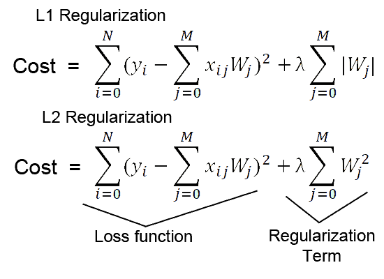
You can create your own custom regularizer class which should be inherited from keras.layers..
					from keras.layers import Layer
from tensorflow.math import reduce_sum, square

class MyActivityRegularizer(Layer):

    def __init__(self, rate=1e-2):
        super(MyActivityRegularizer, self).__init__()
        self.rate = rate

    def call(self, inputs):
        self.add_loss(self.rate * reduce_sum(square(inputs)))
        return inputs
Now, since the regularized loss has been defined, you can simply add it in any built-in layer, or create our own layer.
class SparseMLP(Layer):
  """Stack of Linear layers with our custom regularization loss."""

  def __init__(self, output_dim):
      super(SparseMLP, self).__init__()
      self.dense_1 = layers.Dense(32, activation=tf.nn.relu)
      self.regularization = MyActivityRegularizer(1e-2)
      self.dense_2 = layers.Dense(output_dim)

  def call(self, inputs):
      x = self.dense_1(inputs)
      x = self.regularization(x)
      return self.dense_2(x)
Here custom sparse MLP layer has been defined, where when stacking two linear layers, The custom loss function has been added which will regularize the weights of our deep learning model.
It can be tested:
					mlp = SparseMLP(1)
y = mlp(np.random.normal(size=(10, 10)))

print(mlp.losses)  # List containing one float32 scalar
![]()
It returns a tf.Tensor, which can be converted into numpy using mlp.losses.numpy() method.
Dealing with NaN in Custom Loss in Keras
There are many reasons that our loss function in Keras gives NaN values. If you are new to Keras or practical deep learning, this could be very annoying because you have no idea why Keras is not giving the desired output. Since Keras is a high level API, built over low level frameworks such as Theano, Tensorflow etc. it is difficult to know the problem.
There are many different reasons for which many people have received NaN in their loss, like shown in this figure below
Some of the main reasons, which are very common, are as follows:
1. Missing Values in training dataset
This is one of the most common reasons for why the loss is nan while training. You should remove all the missing values from your dataset, or fill them using a good strategy, such as filling with mean. You can check nan values by using Pandas built in functions.
print(np.any(np.isnan(X_test)))
And if there are any null values, you can either use pandas fillna() function to fill them, or dropna() function to drop those values.
2. Loss is unable to get traction on training dataset
This means that the custom loss function you designed, is not suitable for the dataset, and the business problem you are trying to solve. You should look at the problem from another perspective, and try to find a suitable loss function for your problem.
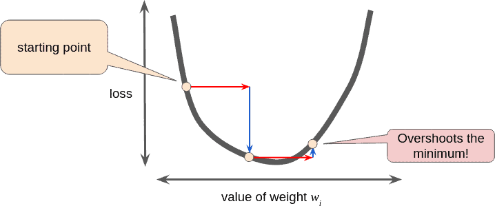
3. Exploding Gradients
Exploding Gradients is a very common problem especially in large neural networks where the value of your gradients become very large. This problem can be solved using Gradient Clipping.
In Keras, you can add gradient clipping to your model when compiling it by adding a parameterclipnorm=x in the selected choice of optimizer. This will clip all the gradients above the value x.
For example:
opt = keras.optimizers.Adam(clipnorm=1.0)
This will clip all the gradients that are greater than 1.0. You can add it into your model as
model.compile(loss=custom_loss, optimizer=opt)
Using RMSProp optimizer function with heavy regularization also helps in diminishing the exploding gradients problem.
4. Dataset is not scaled
Scaling and normalizing the dataset is important. Unscaled data can lead the neural network to behave very strangely. Hence it is advised to properly scale the data.
There are 2 most commonly used scaling methods, and both of them are easily implementable in sklearn which is a famous Machine Learning Library in Python.
- StandardScaler
					from sklearn.preprocessing import StandardScaler
ss = StandardScaler()

X_train_scale = ss.fit_transform(X_train) #using fit_transform so that it can fit on data, and other data can be normalized to same scale
X_test_scale = ss.transform(X_test) #using trasnfrom to get it on same scale as training
5. Dying ReLU problem
A dead ReLU happens, when the relu function always outputs the same value (0 mostly). This means that it takes no role in the discrimination between the inputs. Once a ReLU reaches this state, it is unrecoverable because the function gradient at 0 is also 0, so gradient descent will not change the weights and the model will not improve.
This can be improved by using the Leaky ReLU activation function, where there is a small positive gradient for negative inputs. y=0.01x when x < 0 say
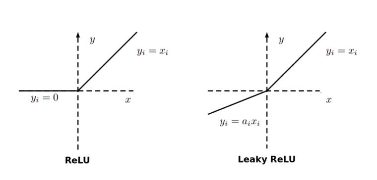
Hence, it is advised to use Leaky ReLU to avoid NaNs in your loss.
In Keras, you can add a leaky relu layer as follows.
keras.layers.LeakyReLU(alpha=0.3, **kwargs)
6. Not a good choice of optimizer function
If you are using Stochastic Gradient Descent, then it is very likely that you are going to face the exploding gradients problem. One way to tackle it is by Scheduling Learning Rate after some epochs, but now due to more advancements and research it has been proven that using a per-parameter adaptive learning rate algorithm like Adam optimizer, you no longer need to schedule the learning rate.
So there are chances that you are not using the right optimizer function.
To use the ADAM optimizer function in Keras, you can use it from keras.optimizers class.
					keras.optimizers.Adam(
    learning_rate=0.001,
    beta_1=0.9,
    beta_2=0.999,
    epsilon=1e-07,
    amsgrad=False,
    name="Adam",
    **kwargs
)
model.compile(optimizer= keras.optimizers.Adam(), loss=custom_loss)
7. Wrong Activation Function
The wrong choice of activation function can also lead to very strange behaviour of the deep learning model. For example if you are working on a multi-class classification problem, and using the relu activation function or sigmoid activation function in the final layer instead of categorical_crossentropy loss function, that can lead the deep learning model to perform very weirdly.
8. Low Batch Size
It has been seen that the optimizer functions on a very low batch size such as 16 or 32 are less stable, as compared to the batch size of 64 or 128.
9. High Learning Rate
High learning rate can lead the deep learning model to not converge to optimum, and it can get lost somewhere in between.
Hence it is advisable to use a lower amount of Learning Rate. It can also be improved using Hyper Parameter Tuning.
10. Different file type (for NLP Problems)
If you are doing some textual problem, you can check your file type by running the following command.
Linux
$ file -i {input}
OSX
$ file -I {input}
This will give you the file type. If that file type is ISO-8859-1 or us-ascii then try converting the file to utf-8 or utf-16le.
Monitoring Keras Loss using Callbacks
It is important to monitor your loss when you are training the model, so that you can understand different types of behaviours your model is showing. There are many callbacks introduced by Keras using which you can monitor the loss. Some of the famous ones are:
1. CSVLogger
CSVLogger is a callback provided by Keras that can be used to save the epoch result in a csv file, so that later on it can be visualized, information could be extracted, and the results of epochs can be stored.
You can use CSVLogger from keras.callbacks.
					from keras.callbacks import CSVLogger

csv_logger = CSVLogger('training.csv')
model.fit(X_train, Y_train, callbacks=[csv_logger])
This will fit the model on the dataset, and stores the callback information in a training.csv file, which you can load in a dataframe and visualize it.
2. TerminateOnNaN
Imagine you set the training limit of your model to 1000 epochs, and your model starts showing NaN loss. You can not just sit and stare at the screen while the progress is 0. Keras provides a TerminateOnNan callback that terminates the training whenever NaN loss is encountered.
					import keras
terNan = keras.callbacks.TerminateOnNaN()
model.fit(X_train, Y_train, callbacks=[terNan])
3. RemoteMonitor
RemoteMonitor is a powerful callback in Keras, which can help us monitor, and visualize the learning in real time.
To use this callback, you need to clone hualos by Francis Chollet, who is the creator of Keras.
					git clone https://github.com/fchollet/hualos
cd hualos
python api.py
Now you can access the hualos at localhost:9000 from your browser. Now you have to define the callback, and add it to your model while training
					monitor = RemoteMonitor()
hist = model.fit( train_X, train_Y, nb_epoch=50, callbacks=[ monitor ] )
During the training, the localhost:9000 is automatically updated, and you can see the visualizations of learning in real time.
4. EarlyStopping
EarlyStopping is a very useful callback provided by Keras, where you can stop the training earlier than expected based on some monitor value.
For example you set your epochs to be 100, and your model is not improving after the 10th epoch. You can not sit and stare at the screen so that model may finish the training, and you can change the architecture of the model. Keras provides EarlyStopping callback, which is used to stop the training based on some criteria.
es = keras.callbacks.EarlyStopping(
    monitor="val_loss",
    patience=3,
)
Here, the EarlyStopping callback has been defined, and the monitor has been set to the validation loss value. And it will check that if the value of validation loss does not improve for 3 epochs, it will stop the training.
This article should give you good foundations in dealing with loss functions, especially in Keras, implementing your own custom loss functions which you develop yourself or a researcher has already developed, and you are implementing that, their implementation using Keras a deep learning framework, avoiding silly errors such as repeating NaNs in your loss function, and how you should monitor your loss function in Keras.
Hopefully, now you have a good grip on these topics:
- What are Loss Functions
- What are Evaluation Metrics?
- Commonly used Loss functions in Keras (Regression and Classification)
- Built-in loss functions in Keras
- What is the custom loss function?
- Why should you use a Custom Loss?
- Implementation of common loss functions in Keras
- Custom Loss Function for Layers i.e Custom Regularization Loss
- Dealing with NaN values in Keras Loss
- Monitoring Keras Loss using callbacks
Built-in loss functions.
View aliases
Main aliases
tf.losses
Classes
class BinaryCrossentropy: Computes the cross-entropy loss between true labels and predicted labels.
class BinaryFocalCrossentropy: Computes the focal cross-entropy loss between true labels and predictions.
class CategoricalCrossentropy: Computes the crossentropy loss between the labels and predictions.
class CategoricalHinge: Computes the categorical hinge loss between y_true & y_pred.
class CosineSimilarity: Computes the cosine similarity between labels and predictions.
class Hinge: Computes the hinge loss between y_true & y_pred.
class Huber: Computes the Huber loss between y_true & y_pred.
class KLDivergence: Computes Kullback-Leibler divergence loss between y_true & y_pred.
class LogCosh: Computes the logarithm of the hyperbolic cosine of the prediction error.
class Loss: Loss base class.
class MeanAbsoluteError: Computes the mean of absolute difference between labels and predictions.
class MeanAbsolutePercentageError: Computes the mean absolute percentage error between y_true & y_pred.
class MeanSquaredError: Computes the mean of squares of errors between labels and predictions.
class MeanSquaredLogarithmicError: Computes the mean squared logarithmic error between y_true & y_pred.
class Poisson: Computes the Poisson loss between y_true & y_pred.
class Reduction: Types of loss reduction.
class SparseCategoricalCrossentropy: Computes the crossentropy loss between the labels and predictions.
class SquaredHinge: Computes the squared hinge loss between y_true & y_pred.
Functions
KLD(...): Computes Kullback-Leibler divergence loss between y_true & y_pred.
MAE(...): Computes the mean absolute error between labels and predictions.
MAPE(...): Computes the mean absolute percentage error between y_true & y_pred.
MSE(...): Computes the mean squared error between labels and predictions.
MSLE(...): Computes the mean squared logarithmic error between y_true & y_pred.
binary_crossentropy(...): Computes the binary crossentropy loss.
binary_focal_crossentropy(...): Computes the binary focal crossentropy loss.
categorical_crossentropy(...): Computes the categorical crossentropy loss.
categorical_hinge(...): Computes the categorical hinge loss between y_true & y_pred.
cosine_similarity(...): Computes the cosine similarity between labels and predictions.
deserialize(...): Deserializes a serialized loss class/function instance.
get(...): Retrieves a Keras loss as a function/Loss class instance.
hinge(...): Computes the hinge loss between y_true & y_pred.
huber(...): Computes Huber loss value.
kl_divergence(...): Computes Kullback-Leibler divergence loss between y_true & y_pred.
kld(...): Computes Kullback-Leibler divergence loss between y_true & y_pred.
kullback_leibler_divergence(...): Computes Kullback-Leibler divergence loss between y_true & y_pred.
log_cosh(...): Logarithm of the hyperbolic cosine of the prediction error.
logcosh(...): Logarithm of the hyperbolic cosine of the prediction error.
mae(...): Computes the mean absolute error between labels and predictions.
mape(...): Computes the mean absolute percentage error between y_true & y_pred.
mean_absolute_error(...): Computes the mean absolute error between labels and predictions.
mean_absolute_percentage_error(...): Computes the mean absolute percentage error between y_true & y_pred.
mean_squared_error(...): Computes the mean squared error between labels and predictions.
mean_squared_logarithmic_error(...): Computes the mean squared logarithmic error between y_true & y_pred.
mse(...): Computes the mean squared error between labels and predictions.
msle(...): Computes the mean squared logarithmic error between y_true & y_pred.
poisson(...): Computes the Poisson loss between y_true and y_pred.
serialize(...): Serializes loss function or Loss instance.
sparse_categorical_crossentropy(...): Computes the sparse categorical crossentropy loss.
squared_hinge(...): Computes the squared hinge loss between y_true & y_pred.
Setup
import tensorflow as tf
from tensorflow import keras
from tensorflow.keras import layers
Introduction
This guide covers training, evaluation, and prediction (inference) models
when using built-in APIs for training & validation (such as Model.fit(),
Model.evaluate() and Model.predict()).
If you are interested in leveraging fit() while specifying your
own training step function, see the
Customizing what happens in fit() guide.
If you are interested in writing your own training & evaluation loops from
scratch, see the guide
«writing a training loop from scratch».
In general, whether you are using built-in loops or writing your own, model training &
evaluation works strictly in the same way across every kind of Keras model —
Sequential models, models built with the Functional API, and models written from
scratch via model subclassing.
This guide doesn’t cover distributed training, which is covered in our
guide to multi-GPU & distributed training.
API overview: a first end-to-end example
When passing data to the built-in training loops of a model, you should either use
NumPy arrays (if your data is small and fits in memory) or tf.data Dataset
objects. In the next few paragraphs, we’ll use the MNIST dataset as NumPy arrays, in
order to demonstrate how to use optimizers, losses, and metrics.
Let’s consider the following model (here, we build in with the Functional API, but it
could be a Sequential model or a subclassed model as well):
inputs = keras.Input(shape=(784,), name="digits")
x = layers.Dense(64, activation="relu", name="dense_1")(inputs)
x = layers.Dense(64, activation="relu", name="dense_2")(x)
outputs = layers.Dense(10, activation="softmax", name="predictions")(x)

model = keras.Model(inputs=inputs, outputs=outputs)
Here’s what the typical end-to-end workflow looks like, consisting of:
- Training
- Validation on a holdout set generated from the original training data
- Evaluation on the test data
We’ll use MNIST data for this example.
(x_train, y_train), (x_test, y_test) = keras.datasets.mnist.load_data()

# Preprocess the data (these are NumPy arrays)
x_train = x_train.reshape(60000, 784).astype("float32") / 255
x_test = x_test.reshape(10000, 784).astype("float32") / 255

y_train = y_train.astype("float32")
y_test = y_test.astype("float32")

# Reserve 10,000 samples for validation
x_val = x_train[-10000:]
y_val = y_train[-10000:]
x_train = x_train[:-10000]
y_train = y_train[:-10000]
We specify the training configuration (optimizer, loss, metrics):
model.compile(
    optimizer=keras.optimizers.RMSprop(),  # Optimizer
    # Loss function to minimize
    loss=keras.losses.SparseCategoricalCrossentropy(),
    # List of metrics to monitor
    metrics=[keras.metrics.SparseCategoricalAccuracy()],
)
We call fit(), which will train the model by slicing the data into «batches» of size
batch_size, and repeatedly iterating over the entire dataset for a given number of
epochs.
print("Fit model on training data")
history = model.fit(
    x_train,
    y_train,
    batch_size=64,
    epochs=2,
    # We pass some validation for
    # monitoring validation loss and metrics
    # at the end of each epoch
    validation_data=(x_val, y_val),
)
Fit model on training data
Epoch 1/2
782/782 [==============================] - 3s 3ms/step - loss: 0.3387 - sparse_categorical_accuracy: 0.9050 - val_loss: 0.1957 - val_sparse_categorical_accuracy: 0.9426
Epoch 2/2
782/782 [==============================] - 2s 3ms/step - loss: 0.1543 - sparse_categorical_accuracy: 0.9548 - val_loss: 0.1425 - val_sparse_categorical_accuracy: 0.9593
The returned history object holds a record of the loss values and metric values
during training:
history.history
{'loss': [0.3386789858341217, 0.1543138176202774],
 'sparse_categorical_accuracy': [0.9050400257110596, 0.9548400044441223],
 'val_loss': [0.19569723308086395, 0.14253544807434082],
 'val_sparse_categorical_accuracy': [0.9426000118255615, 0.9592999815940857]}
We evaluate the model on the test data via evaluate():
# Evaluate the model on the test data using `evaluate`
print("Evaluate on test data")
results = model.evaluate(x_test, y_test, batch_size=128)
print("test loss, test acc:", results)

# Generate predictions (probabilities -- the output of the last layer)
# on new data using `predict`
print("Generate predictions for 3 samples")
predictions = model.predict(x_test[:3])
print("predictions shape:", predictions.shape)
Evaluate on test data
79/79 [==============================] - 0s 2ms/step - loss: 0.1414 - sparse_categorical_accuracy: 0.9569
test loss, test acc: [0.14140386879444122, 0.9569000005722046]
Generate predictions for 3 samples
predictions shape: (3, 10)
Now, let’s review each piece of this workflow in detail.
The compile() method: specifying a loss, metrics, and an optimizer
To train a model with fit(), you need to specify a loss function, an optimizer, and
optionally, some metrics to monitor.
You pass these to the model as arguments to the compile() method:
model.compile(
    optimizer=keras.optimizers.RMSprop(learning_rate=1e-3),
    loss=keras.losses.SparseCategoricalCrossentropy(),
    metrics=[keras.metrics.SparseCategoricalAccuracy()],
)
The metrics argument should be a list — your model can have any number of metrics.
If your model has multiple outputs, you can specify different losses and metrics for
each output, and you can modulate the contribution of each output to the total loss of
the model. You will find more details about this in the Passing data to multi-input,
multi-output models section.
Note that if you’re satisfied with the default settings, in many cases the optimizer,
loss, and metrics can be specified via string identifiers as a shortcut:
model.compile(
    optimizer="rmsprop",
    loss="sparse_categorical_crossentropy",
    metrics=["sparse_categorical_accuracy"],
)
For later reuse, let’s put our model definition and compile step in functions; we will
call them several times across different examples in this guide.
def get_uncompiled_model():
    inputs = keras.Input(shape=(784,), name="digits")
    x = layers.Dense(64, activation="relu", name="dense_1")(inputs)
    x = layers.Dense(64, activation="relu", name="dense_2")(x)
    outputs = layers.Dense(10, activation="softmax", name="predictions")(x)
    model = keras.Model(inputs=inputs, outputs=outputs)
    return model


def get_compiled_model():
    model = get_uncompiled_model()
    model.compile(
        optimizer="rmsprop",
        loss="sparse_categorical_crossentropy",
        metrics=["sparse_categorical_accuracy"],
    )
    return model
Many built-in optimizers, losses, and metrics are available
In general, you won’t have to create your own losses, metrics, or optimizers
from scratch, because what you need is likely to be already part of the Keras API:
Optimizers:
SGD()(with or without momentum)RMSprop()Adam()- etc.
Losses:
MeanSquaredError()KLDivergence()CosineSimilarity()- etc.
Metrics:
AUC()Precision()Recall()- etc.
Custom losses
If you need to create a custom loss, Keras provides two ways to do so.
The first method involves creating a function that accepts inputs y_true and
y_pred. The following example shows a loss function that computes the mean squared
error between the real data and the predictions:
def custom_mean_squared_error(y_true, y_pred):
    return tf.math.reduce_mean(tf.square(y_true - y_pred))


model = get_uncompiled_model()
model.compile(optimizer=keras.optimizers.Adam(), loss=custom_mean_squared_error)

# We need to one-hot encode the labels to use MSE
y_train_one_hot = tf.one_hot(y_train, depth=10)
model.fit(x_train, y_train_one_hot, batch_size=64, epochs=1)
782/782 [==============================] - 2s 2ms/step - loss: 0.0162
<keras.callbacks.History at 0x7ff8881ba250>
If you need a loss function that takes in parameters beside y_true and y_pred, you
can subclass the tf.keras.losses.Loss class and implement the following two methods:
__init__(self): accept parameters to pass during the call of your loss functioncall(self, y_true, y_pred): use the targets (y_true) and the model predictions
(y_pred) to compute the model’s loss
Let’s say you want to use mean squared error, but with an added term that
will de-incentivize prediction values far from 0.5 (we assume that the categorical
targets are one-hot encoded and take values between 0 and 1). This
creates an incentive for the model not to be too confident, which may help
reduce overfitting (we won’t know if it works until we try!).
Here’s how you would do it:
class CustomMSE(keras.losses.Loss):
    def __init__(self, regularization_factor=0.1, name="custom_mse"):
        super().__init__(name=name)
        self.regularization_factor = regularization_factor

    def call(self, y_true, y_pred):
        mse = tf.math.reduce_mean(tf.square(y_true - y_pred))
        reg = tf.math.reduce_mean(tf.square(0.5 - y_pred))
        return mse + reg * self.regularization_factor


model = get_uncompiled_model()
model.compile(optimizer=keras.optimizers.Adam(), loss=CustomMSE())

y_train_one_hot = tf.one_hot(y_train, depth=10)
model.fit(x_train, y_train_one_hot, batch_size=64, epochs=1)
782/782 [==============================] - 2s 2ms/step - loss: 0.0388
<keras.callbacks.History at 0x7ff8882130d0>
Custom metrics
If you need a metric that isn’t part of the API, you can easily create custom metrics
by subclassing the tf.keras.metrics.Metric class. You will need to implement 4
methods:
__init__(self), in which you will create state variables for your metric.update_state(self, y_true, y_pred, sample_weight=None), which uses the targets
y_true and the model predictions y_pred to update the state variables.result(self), which uses the state variables to compute the final results.reset_state(self), which reinitializes the state of the metric.
State update and results computation are kept separate (in update_state() and
result(), respectively) because in some cases, the results computation might be very
expensive and would only be done periodically.
Here’s a simple example showing how to implement a CategoricalTruePositives metric
that counts how many samples were correctly classified as belonging to a given class:
class CategoricalTruePositives(keras.metrics.Metric):
def __init__(self, name="categorical_true_positives", **kwargs):
super(CategoricalTruePositives, self).__init__(name=name, **kwargs)
self.true_positives = self.add_weight(name="ctp", initializer="zeros")
def update_state(self, y_true, y_pred, sample_weight=None):
y_pred = tf.reshape(tf.argmax(y_pred, axis=1), shape=(-1, 1))
values = tf.cast(y_true, "int32") == tf.cast(y_pred, "int32")
values = tf.cast(values, "float32")
if sample_weight is not None:
sample_weight = tf.cast(sample_weight, "float32")
values = tf.multiply(values, sample_weight)
self.true_positives.assign_add(tf.reduce_sum(values))
def result(self):
return self.true_positives
def reset_state(self):
# The state of the metric will be reset at the start of each epoch.
self.true_positives.assign(0.0)
model = get_uncompiled_model()
model.compile(
optimizer=keras.optimizers.RMSprop(learning_rate=1e-3),
loss=keras.losses.SparseCategoricalCrossentropy(),
metrics=[CategoricalTruePositives()],
)
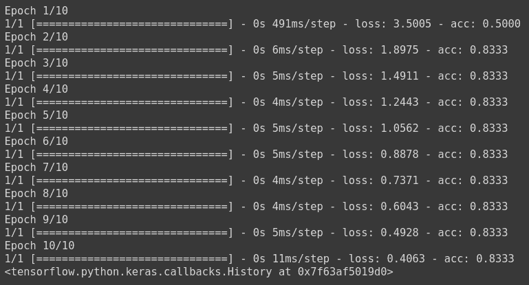
model.fit(x_train, y_train, batch_size=64, epochs=3)
Epoch 1/3
782/782 [==============================] - 2s 3ms/step - loss: 0.3404 - categorical_true_positives: 45217.0000
Epoch 2/3
782/782 [==============================] - 2s 3ms/step - loss: 0.1588 - categorical_true_positives: 47606.0000
Epoch 3/3
782/782 [==============================] - 2s 3ms/step - loss: 0.1168 - categorical_true_positives: 48278.0000
<keras.callbacks.History at 0x7ff8880a3610>
Handling losses and metrics that don’t fit the standard signature
The overwhelming majority of losses and metrics can be computed from y_true and
y_pred, where y_pred is an output of your model — but not all of them. For
instance, a regularization loss may only require the activation of a layer (there are
no targets in this case), and this activation may not be a model output.
In such cases, you can call self.add_loss(loss_value) from inside the call method of
a custom layer. Losses added in this way get added to the «main» loss during training
(the one passed to compile()). Here’s a simple example that adds activity
regularization (note that activity regularization is built-in in all Keras layers —
this layer is just for the sake of providing a concrete example):
class ActivityRegularizationLayer(layers.Layer):
    def call(self, inputs):
        self.add_loss(tf.reduce_sum(inputs) * 0.1)
        return inputs  # Pass-through layer.


inputs = keras.Input(shape=(784,), name="digits")
x = layers.Dense(64, activation="relu", name="dense_1")(inputs)

# Insert activity regularization as a layer
x = ActivityRegularizationLayer()(x)

x = layers.Dense(64, activation="relu", name="dense_2")(x)
outputs = layers.Dense(10, name="predictions")(x)

model = keras.Model(inputs=inputs, outputs=outputs)
model.compile(
    optimizer=keras.optimizers.RMSprop(learning_rate=1e-3),
    loss=keras.losses.SparseCategoricalCrossentropy(from_logits=True),
)

# The displayed loss will be much higher than before
# due to the regularization component.
model.fit(x_train, y_train, batch_size=64, epochs=1)
782/782 [==============================] - 2s 2ms/step - loss: 2.4545
<keras.callbacks.History at 0x7ff87c53f310>
You can do the same for logging metric values, using add_metric():
class MetricLoggingLayer(layers.Layer):
    def call(self, inputs):
        # The `aggregation` argument defines
        # how to aggregate the per-batch values
        # over each epoch:
        # in this case we simply average them.
        self.add_metric(
            keras.backend.std(inputs), name="std_of_activation", aggregation="mean"
        )
        return inputs  # Pass-through layer.


inputs = keras.Input(shape=(784,), name="digits")
x = layers.Dense(64, activation="relu", name="dense_1")(inputs)

# Insert std logging as a layer.
x = MetricLoggingLayer()(x)

x = layers.Dense(64, activation="relu", name="dense_2")(x)
outputs = layers.Dense(10, name="predictions")(x)

model = keras.Model(inputs=inputs, outputs=outputs)
model.compile(
    optimizer=keras.optimizers.RMSprop(learning_rate=1e-3),
    loss=keras.losses.SparseCategoricalCrossentropy(from_logits=True),
)
model.fit(x_train, y_train, batch_size=64, epochs=1)
782/782 [==============================] - 2s 2ms/step - loss: 0.3461 - std_of_activation: 0.9929
<keras.callbacks.History at 0x7ff87c3d5bd0>
In the Functional API,
you can also call model.add_loss(loss_tensor),
or model.add_metric(metric_tensor, name, aggregation).
Here’s a simple example:
inputs = keras.Input(shape=(784,), name="digits")
x1 = layers.Dense(64, activation="relu", name="dense_1")(inputs)
x2 = layers.Dense(64, activation="relu", name="dense_2")(x1)
outputs = layers.Dense(10, name="predictions")(x2)
model = keras.Model(inputs=inputs, outputs=outputs)

model.add_loss(tf.reduce_sum(x1) * 0.1)

model.add_metric(keras.backend.std(x1), name="std_of_activation", aggregation="mean")

model.compile(
    optimizer=keras.optimizers.RMSprop(1e-3),
    loss=keras.losses.SparseCategoricalCrossentropy(from_logits=True),
)
model.fit(x_train, y_train, batch_size=64, epochs=1)
782/782 [==============================] - 2s 3ms/step - loss: 2.4647 - std_of_activation: 0.0017
<keras.callbacks.History at 0x7ff87c216f90>
Note that when you pass losses via add_loss(), it becomes possible to call
compile() without a loss function, since the model already has a loss to minimize.
Consider the following LogisticEndpoint layer: it takes as inputs
targets & logits, and it tracks a crossentropy loss via add_loss(). It also
tracks classification accuracy via add_metric().
class LogisticEndpoint(keras.layers.Layer):
    def __init__(self, name=None):
        super(LogisticEndpoint, self).__init__(name=name)
        self.loss_fn = keras.losses.BinaryCrossentropy(from_logits=True)
        self.accuracy_fn = keras.metrics.BinaryAccuracy()

    def call(self, targets, logits, sample_weights=None):
        # Compute the training-time loss value and add it
        # to the layer using `self.add_loss()`.
        loss = self.loss_fn(targets, logits, sample_weights)
        self.add_loss(loss)

        # Log accuracy as a metric and add it
        # to the layer using `self.add_metric()`.
        acc = self.accuracy_fn(targets, logits, sample_weights)
        self.add_metric(acc, name="accuracy")

        # Return the inference-time prediction tensor (for `.predict()`).
        return tf.nn.softmax(logits)
You can use it in a model with two inputs (input data & targets), compiled without a
loss argument, like this:
import numpy as np

inputs = keras.Input(shape=(3,), name="inputs")
targets = keras.Input(shape=(10,), name="targets")
logits = keras.layers.Dense(10)(inputs)
predictions = LogisticEndpoint(name="predictions")(logits, targets)

model = keras.Model(inputs=[inputs, targets], outputs=predictions)
model.compile(optimizer="adam")  # No loss argument!

data = {
    "inputs": np.random.random((3, 3)),
    "targets": np.random.random((3, 10)),
}
model.fit(data)
1/1 [==============================] - 0s 414ms/step - loss: 0.9889 - binary_accuracy: 0.0000e+00
<keras.callbacks.History at 0x7ff87c0848d0>
For more information about training multi-input models, see the section Passing data
to multi-input, multi-output models.
Automatically setting apart a validation holdout set
In the first end-to-end example you saw, we used the validation_data argument to pass
a tuple of NumPy arrays (x_val, y_val) to the model for evaluating a validation loss
and validation metrics at the end of each epoch.
Here’s another option: the argument validation_split allows you to automatically
reserve part of your training data for validation. The argument value represents the
fraction of the data to be reserved for validation, so it should be set to a number
higher than 0 and lower than 1. For instance, validation_split=0.2 means «use 20% of
the data for validation», and validation_split=0.6 means «use 60% of the data for
validation».
The way the validation is computed is by taking the last x% samples of the arrays
received by the fit() call, before any shuffling.
Note that you can only use validation_split when training with NumPy data.
model = get_compiled_model()
model.fit(x_train, y_train, batch_size=64, validation_split=0.2, epochs=1)
625/625 [==============================] - 2s 3ms/step - loss: 0.3682 - sparse_categorical_accuracy: 0.8957 - val_loss: 0.2276 - val_sparse_categorical_accuracy: 0.9301
<keras.callbacks.History at 0x7ff81c680890>
Training & evaluation from tf.data Datasets
In the past few paragraphs, you’ve seen how to handle losses, metrics, and optimizers,
and you’ve seen how to use the validation_data and validation_split arguments in
fit(), when your data is passed as NumPy arrays.
Let’s now take a look at the case where your data comes in the form of a
tf.data.Dataset object.
The tf.data API is a set of utilities in TensorFlow 2.0 for loading and preprocessing
data in a way that’s fast and scalable.
For a complete guide about creating Datasets, see the
tf.data documentation.
You can pass a Dataset instance directly to the methods fit(), evaluate(), and
predict():
model = get_compiled_model()

# First, let's create a training Dataset instance.
# For the sake of our example, we'll use the same MNIST data as before.
train_dataset = tf.data.Dataset.from_tensor_slices((x_train, y_train))
# Shuffle and slice the dataset.
train_dataset = train_dataset.shuffle(buffer_size=1024).batch(64)

# Now we get a test dataset.
test_dataset = tf.data.Dataset.from_tensor_slices((x_test, y_test))
test_dataset = test_dataset.batch(64)

# Since the dataset already takes care of batching,
# we don't pass a `batch_size` argument.
model.fit(train_dataset, epochs=3)

# You can also evaluate or predict on a dataset.
print("Evaluate")
result = model.evaluate(test_dataset)
dict(zip(model.metrics_names, result))
Epoch 1/3
782/782 [==============================] - 2s 3ms/step - loss: 0.3372 - sparse_categorical_accuracy: 0.9047
Epoch 2/3
782/782 [==============================] - 2s 3ms/step - loss: 0.1596 - sparse_categorical_accuracy: 0.9523
Epoch 3/3
782/782 [==============================] - 2s 3ms/step - loss: 0.1171 - sparse_categorical_accuracy: 0.9655
Evaluate
157/157 [==============================] - 0s 2ms/step - loss: 0.1211 - sparse_categorical_accuracy: 0.9648
{'loss': 0.12107347697019577,
 'sparse_categorical_accuracy': 0.9648000001907349}
Note that the Dataset is reset at the end of each epoch, so it can be reused of the
next epoch.
If you want to run training only on a specific number of batches from this Dataset, you
can pass the steps_per_epoch argument, which specifies how many training steps the
model should run using this Dataset before moving on to the next epoch.
If you do this, the dataset is not reset at the end of each epoch, instead we just keep
drawing the next batches. The dataset will eventually run out of data (unless it is an
infinitely-looping dataset).
model = get_compiled_model()

# Prepare the training dataset
train_dataset = tf.data.Dataset.from_tensor_slices((x_train, y_train))
train_dataset = train_dataset.shuffle(buffer_size=1024).batch(64)

# Only use the 100 batches per epoch (that's 64 * 100 samples)
model.fit(train_dataset, epochs=3, steps_per_epoch=100)
Epoch 1/3
100/100 [==============================] - 1s 3ms/step - loss: 0.7937 - sparse_categorical_accuracy: 0.7894
Epoch 2/3
100/100 [==============================] - 0s 3ms/step - loss: 0.3699 - sparse_categorical_accuracy: 0.8938
Epoch 3/3
100/100 [==============================] - 0s 3ms/step - loss: 0.3155 - sparse_categorical_accuracy: 0.9061
<keras.callbacks.History at 0x7ff81c587e90>
Using a validation dataset
You can pass a Dataset instance as the validation_data argument in fit():
model = get_compiled_model()

# Prepare the training dataset
train_dataset = tf.data.Dataset.from_tensor_slices((x_train, y_train))
train_dataset = train_dataset.shuffle(buffer_size=1024).batch(64)

# Prepare the validation dataset
val_dataset = tf.data.Dataset.from_tensor_slices((x_val, y_val))
val_dataset = val_dataset.batch(64)

model.fit(train_dataset, epochs=1, validation_data=val_dataset)
782/782 [==============================] - 3s 3ms/step - loss: 0.3380 - sparse_categorical_accuracy: 0.9035 - val_loss: 0.2015 - val_sparse_categorical_accuracy: 0.9405
<keras.callbacks.History at 0x7ff81c30e450>
At the end of each epoch, the model will iterate over the validation dataset and
compute the validation loss and validation metrics.
If you want to run validation only on a specific number of batches from this dataset,
you can pass the validation_steps argument, which specifies how many validation
steps the model should run with the validation dataset before interrupting validation
and moving on to the next epoch:
model = get_compiled_model()

# Prepare the training dataset
train_dataset = tf.data.Dataset.from_tensor_slices((x_train, y_train))
train_dataset = train_dataset.shuffle(buffer_size=1024).batch(64)

# Prepare the validation dataset
val_dataset = tf.data.Dataset.from_tensor_slices((x_val, y_val))
val_dataset = val_dataset.batch(64)

model.fit(
    train_dataset,
    epochs=1,
    # Only run validation using the first 10 batches of the dataset
    # using the `validation_steps` argument
    validation_data=val_dataset,
    validation_steps=10,
)
782/782 [==============================] - 3s 3ms/step - loss: 0.3369 - sparse_categorical_accuracy: 0.9036 - val_loss: 0.2953 - val_sparse_categorical_accuracy: 0.9187
<keras.callbacks.History at 0x7ff81c30e310>
Note that the validation dataset will be reset after each use (so that you will always
be evaluating on the same samples from epoch to epoch).
The argument validation_split (generating a holdout set from the training data) is
not supported when training from Dataset objects, since this feature requires the
ability to index the samples of the datasets, which is not possible in general with
the Dataset API.
Other input formats supported
Besides NumPy arrays, eager tensors, and TensorFlow Datasets, it’s possible to train
a Keras model using Pandas dataframes, or from Python generators that yield batches of
data & labels.
In particular, the keras.utils.Sequence class offers a simple interface to build
Python data generators that are multiprocessing-aware and can be shuffled.
In general, we recommend that you use:
- NumPy input data if your data is small and fits in memory
Datasetobjects if you have large datasets and you need to do distributed trainingSequenceobjects if you have large datasets and you need to do a lot of custom
Python-side processing that cannot be done in TensorFlow (e.g. if you rely on external libraries
for data loading or preprocessing).
Using a keras.utils.Sequence object as input
keras.utils.Sequence is a utility that you can subclass to obtain a Python generator with
two important properties:
- It works well with multiprocessing.
- It can be shuffled (e.g. when passing
shuffle=Trueinfit()).
A Sequence must implement two methods:
__getitem____len__
The method __getitem__ should return a complete batch.
If you want to modify your dataset between epochs, you may implement on_epoch_end.
Here’s a quick example:
from skimage.io import imread
from skimage.transform import resize
import numpy as np

# Here, `filenames` is list of path to the images
# and `labels` are the associated labels.

class CIFAR10Sequence(Sequence):
    def __init__(self, filenames, labels, batch_size):
        self.filenames, self.labels = filenames, labels
        self.batch_size = batch_size

    def __len__(self):
        return int(np.ceil(len(self.filenames) / float(self.batch_size)))

    def __getitem__(self, idx):
        batch_x = self.filenames[idx * self.batch_size:(idx + 1) * self.batch_size]
        batch_y = self.labels[idx * self.batch_size:(idx + 1) * self.batch_size]
        return np.array([
            resize(imread(filename), (200, 200))
               for filename in batch_x]), np.array(batch_y)

sequence = CIFAR10Sequence(filenames, labels, batch_size)
model.fit(sequence, epochs=10)
Using sample weighting and class weighting
With the default settings the weight of a sample is decided by its frequency
in the dataset. There are two methods to weight the data, independent of
sample frequency:
- Class weights
- Sample weights
Class weights
This is set by passing a dictionary to the class_weight argument to
Model.fit(). This dictionary maps class indices to the weight that should
be used for samples belonging to this class.
This can be used to balance classes without resampling, or to train a
model that gives more importance to a particular class.
For instance, if class «0» is half as represented as class «1» in your data,
you could use Model.fit(..., class_weight={0: 1., 1: 0.5}).
Here’s a NumPy example where we use class weights or sample weights to
give more importance to the correct classification of class #5 (which
is the digit «5» in the MNIST dataset).
import numpy as np

class_weight = {
    0: 1.0,
    1: 1.0,
    2: 1.0,
    3: 1.0,
    4: 1.0,
    # Set weight "2" for class "5",
    # making this class 2x more important
    5: 2.0,
    6: 1.0,
    7: 1.0,
    8: 1.0,
    9: 1.0,
}

print("Fit with class weight")
model = get_compiled_model()
model.fit(x_train, y_train, class_weight=class_weight, batch_size=64, epochs=1)
Fit with class weight
782/782 [==============================] - 2s 3ms/step - loss: 0.3708 - sparse_categorical_accuracy: 0.9032
<keras.callbacks.History at 0x7ff80c7ddd10>
Sample weights
For fine grained control, or if you are not building a classifier,
you can use «sample weights».
- When training from NumPy data: Pass the
sample_weight
argument toModel.fit(). - When training from
tf.dataor any other sort of iterator:
Yield(input_batch, label_batch, sample_weight_batch)tuples.
A «sample weights» array is an array of numbers that specify how much weight
each sample in a batch should have in computing the total loss. It is commonly
used in imbalanced classification problems (the idea being to give more weight
to rarely-seen classes).
When the weights used are ones and zeros, the array can be used as a mask for
the loss function (entirely discarding the contribution of certain samples to
the total loss).
sample_weight = np.ones(shape=(len(y_train),))
sample_weight[y_train == 5] = 2.0

print("Fit with sample weight")
model = get_compiled_model()
model.fit(x_train, y_train, sample_weight=sample_weight, batch_size=64, epochs=1)
Fit with sample weight
782/782 [==============================] - 2s 3ms/step - loss: 0.3806 - sparse_categorical_accuracy: 0.9000
<keras.callbacks.History at 0x7ff80c650350>
Here’s a matching Dataset example:
sample_weight = np.ones(shape=(len(y_train),))
sample_weight[y_train == 5] = 2.0

# Create a Dataset that includes sample weights
# (3rd element in the return tuple).
train_dataset = tf.data.Dataset.from_tensor_slices((x_train, y_train, sample_weight))

# Shuffle and slice the dataset.
train_dataset = train_dataset.shuffle(buffer_size=1024).batch(64)

model = get_compiled_model()
model.fit(train_dataset, epochs=1)
782/782 [==============================] - 3s 3ms/step - loss: 0.3588 - sparse_categorical_accuracy: 0.9070
<keras.callbacks.History at 0x7ff80c51cb50>
Passing data to multi-input, multi-output models
In the previous examples, we were considering a model with a single input (a tensor of
shape (764,)) and a single output (a prediction tensor of shape (10,)). But what
about models that have multiple inputs or outputs?
Consider the following model, which has an image input of shape (32, 32, 3) (that’s
(height, width, channels)) and a time series input of shape (None, 10) (that’s
(timesteps, features)). Our model will have two outputs computed from the
combination of these inputs: a «score» (of shape (1,)) and a probability
distribution over five classes (of shape (5,)).
image_input = keras.Input(shape=(32, 32, 3), name="img_input")
timeseries_input = keras.Input(shape=(None, 10), name="ts_input")

x1 = layers.Conv2D(3, 3)(image_input)
x1 = layers.GlobalMaxPooling2D()(x1)

x2 = layers.Conv1D(3, 3)(timeseries_input)
x2 = layers.GlobalMaxPooling1D()(x2)

x = layers.concatenate([x1, x2])

score_output = layers.Dense(1, name="score_output")(x)
class_output = layers.Dense(5, name="class_output")(x)

model = keras.Model(
    inputs=[image_input, timeseries_input], outputs=[score_output, class_output]
)
Let’s plot this model, so you can clearly see what we’re doing here (note that the
shapes shown in the plot are batch shapes, rather than per-sample shapes).
keras.utils.plot_model(model, "multi_input_and_output_model.png", show_shapes=True)
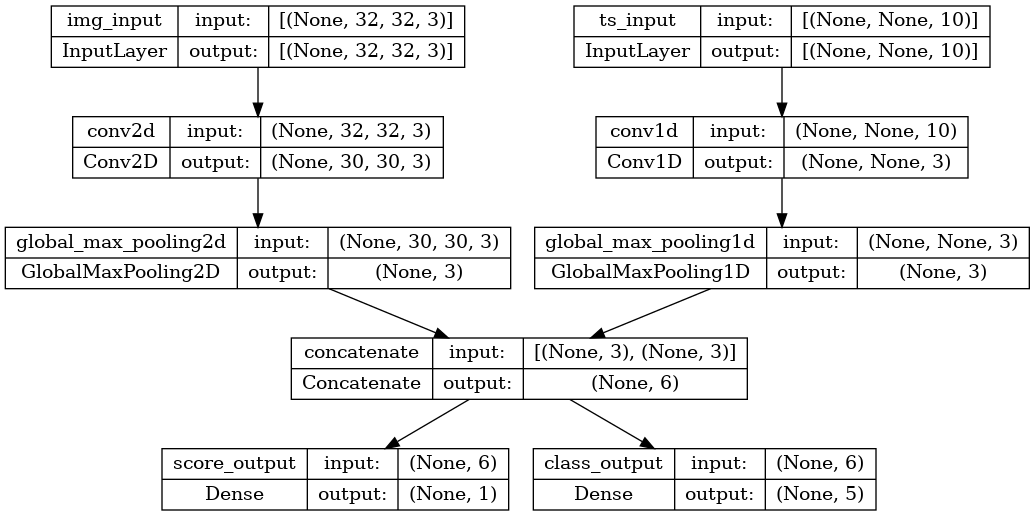
At compilation time, we can specify different losses to different outputs, by passing
the loss functions as a list:
model.compile(
    optimizer=keras.optimizers.RMSprop(1e-3),
    loss=[keras.losses.MeanSquaredError(), keras.losses.CategoricalCrossentropy()],
)
If we only passed a single loss function to the model, the same loss function would be
applied to every output (which is not appropriate here).
Likewise for metrics:
model.compile(
    optimizer=keras.optimizers.RMSprop(1e-3),
    loss=[keras.losses.MeanSquaredError(), keras.losses.CategoricalCrossentropy()],
    metrics=[
        [
            keras.metrics.MeanAbsolutePercentageError(),
            keras.metrics.MeanAbsoluteError(),
        ],
        [keras.metrics.CategoricalAccuracy()],
    ],
)
Since we gave names to our output layers, we could also specify per-output losses and
metrics via a dict:
model.compile(
    optimizer=keras.optimizers.RMSprop(1e-3),
    loss={
        "score_output": keras.losses.MeanSquaredError(),
        "class_output": keras.losses.CategoricalCrossentropy(),
    },
    metrics={
        "score_output": [
            keras.metrics.MeanAbsolutePercentageError(),
            keras.metrics.MeanAbsoluteError(),
        ],
        "class_output": [keras.metrics.CategoricalAccuracy()],
    },
)
We recommend the use of explicit names and dicts if you have more than 2 outputs.
It’s possible to give different weights to different output-specific losses (for
instance, one might wish to privilege the «score» loss in our example, by giving to 2x
the importance of the class loss), using the loss_weights argument:
model.compile(
    optimizer=keras.optimizers.RMSprop(1e-3),
    loss={
        "score_output": keras.losses.MeanSquaredError(),
        "class_output": keras.losses.CategoricalCrossentropy(),
    },
    metrics={
        "score_output": [
            keras.metrics.MeanAbsolutePercentageError(),
            keras.metrics.MeanAbsoluteError(),
        ],
        "class_output": [keras.metrics.CategoricalAccuracy()],
    },
    loss_weights={"score_output": 2.0, "class_output": 1.0},
)
You could also choose not to compute a loss for certain outputs, if these outputs are
meant for prediction but not for training:
# List loss version
model.compile(
    optimizer=keras.optimizers.RMSprop(1e-3),
    loss=[None, keras.losses.CategoricalCrossentropy()],
)

# Or dict loss version
model.compile(
    optimizer=keras.optimizers.RMSprop(1e-3),
    loss={"class_output": keras.losses.CategoricalCrossentropy()},
)
Passing data to a multi-input or multi-output model in fit() works in a similar way as
specifying a loss function in compile: you can pass lists of NumPy arrays (with
1:1 mapping to the outputs that received a loss function) or dicts mapping output
names to NumPy arrays.
model.compile(
    optimizer=keras.optimizers.RMSprop(1e-3),
    loss=[keras.losses.MeanSquaredError(), keras.losses.CategoricalCrossentropy()],
)

# Generate dummy NumPy data
img_data = np.random.random_sample(size=(100, 32, 32, 3))
ts_data = np.random.random_sample(size=(100, 20, 10))
score_targets = np.random.random_sample(size=(100, 1))
class_targets = np.random.random_sample(size=(100, 5))

# Fit on lists
model.fit([img_data, ts_data], [score_targets, class_targets], batch_size=32, epochs=1)

# Alternatively, fit on dicts
model.fit(
    {"img_input": img_data, "ts_input": ts_data},
    {"score_output": score_targets, "class_output": class_targets},
    batch_size=32,
    epochs=1,
)
4/4 [==============================] - 2s 9ms/step - loss: 5.6917 - score_output_loss: 0.1031 - class_output_loss: 5.5886
4/4 [==============================] - 0s 6ms/step - loss: 4.4108 - score_output_loss: 0.0999 - class_output_loss: 4.3109
<keras.callbacks.History at 0x7ff80c3b4110>
Here’s the Dataset use case: similarly as what we did for NumPy arrays, the Dataset
should return a tuple of dicts.
train_dataset = tf.data.Dataset.from_tensor_slices(
    (
        {"img_input": img_data, "ts_input": ts_data},
        {"score_output": score_targets, "class_output": class_targets},
    )
)
train_dataset = train_dataset.shuffle(buffer_size=1024).batch(64)

model.fit(train_dataset, epochs=1)
2/2 [==============================] - 0s 21ms/step - loss: 4.2451 - score_output_loss: 0.0993 - class_output_loss: 4.1458
<keras.callbacks.History at 0x7ff80c3ed450>
Using callbacks
Callbacks in Keras are objects that are called at different points during training (at
the start of an epoch, at the end of a batch, at the end of an epoch, etc.). They
can be used to implement certain behaviors, such as:
- Doing validation at different points during training (beyond the built-in per-epoch
validation) - Checkpointing the model at regular intervals or when it exceeds a certain accuracy
threshold - Changing the learning rate of the model when training seems to be plateauing
- Doing fine-tuning of the top layers when training seems to be plateauing
- Sending email or instant message notifications when training ends or where a certain
performance threshold is exceeded - Etc.
Callbacks can be passed as a list to your call to fit():
model = get_compiled_model()

callbacks = [
    keras.callbacks.EarlyStopping(
        # Stop training when `val_loss` is no longer improving
        monitor="val_loss",
        # "no longer improving" being defined as "no better than 1e-2 less"
        min_delta=1e-2,
        # "no longer improving" being further defined as "for at least 2 epochs"
        patience=2,
        verbose=1,
    )
]
model.fit(
    x_train,
    y_train,
    epochs=20,
    batch_size=64,
    callbacks=callbacks,
    validation_split=0.2,
)
Epoch 1/20
625/625 [==============================] - 2s 3ms/step - loss: 0.3725 - sparse_categorical_accuracy: 0.8939 - val_loss: 0.2314 - val_sparse_categorical_accuracy: 0.9321
Epoch 2/20
625/625 [==============================] - 2s 3ms/step - loss: 0.1805 - sparse_categorical_accuracy: 0.9471 - val_loss: 0.2012 - val_sparse_categorical_accuracy: 0.9379
Epoch 3/20
625/625 [==============================] - 2s 3ms/step - loss: 0.1346 - sparse_categorical_accuracy: 0.9603 - val_loss: 0.1651 - val_sparse_categorical_accuracy: 0.9505
Epoch 4/20
625/625 [==============================] - 2s 3ms/step - loss: 0.1065 - sparse_categorical_accuracy: 0.9684 - val_loss: 0.1510 - val_sparse_categorical_accuracy: 0.9571
Epoch 5/20
625/625 [==============================] - 2s 3ms/step - loss: 0.0884 - sparse_categorical_accuracy: 0.9734 - val_loss: 0.1505 - val_sparse_categorical_accuracy: 0.9538
Epoch 6/20
625/625 [==============================] - 2s 3ms/step - loss: 0.0746 - sparse_categorical_accuracy: 0.9778 - val_loss: 0.1508 - val_sparse_categorical_accuracy: 0.9575
Epoch 00006: early stopping
<keras.callbacks.History at 0x7ff80c64cad0>
Many built-in callbacks are available
There are many built-in callbacks already available in Keras, such as:
ModelCheckpoint: Periodically save the model.EarlyStopping: Stop training when training is no longer improving the validation
metrics.TensorBoard: periodically write model logs that can be visualized in
TensorBoard (more details in the section
«Visualization»).CSVLogger: streams loss and metrics data to a CSV file.- etc.
See the callbacks documentation for the complete list.
Writing your own callback
You can create a custom callback by extending the base class
keras.callbacks.Callback. A callback has access to its associated model through the
class property self.model.
Make sure to read the
complete guide to writing custom callbacks.
Here’s a simple example saving a list of per-batch loss values during training:
class LossHistory(keras.callbacks.Callback):
    def on_train_begin(self, logs):
        self.per_batch_losses = []

    def on_batch_end(self, batch, logs):
        self.per_batch_losses.append(logs.get("loss"))
Checkpointing models
When you’re training model on relatively large datasets, it’s crucial to save
checkpoints of your model at frequent intervals.
The easiest way to achieve this is with the ModelCheckpoint callback:
model = get_compiled_model()

callbacks = [
    keras.callbacks.ModelCheckpoint(
        # Path where to save the model
        # The two parameters below mean that we will overwrite
        # the current checkpoint if and only if
        # the `val_loss` score has improved.
        # The saved model name will include the current epoch.
        filepath="mymodel_{epoch}",
        save_best_only=True,  # Only save a model if `val_loss` has improved.
        monitor="val_loss",
        verbose=1,
    )
]
model.fit(
    x_train, y_train, epochs=2, batch_size=64, callbacks=callbacks, validation_split=0.2
)
Epoch 1/2
613/625 [============================>.] - ETA: 0s - loss: 0.3693 - sparse_categorical_accuracy: 0.8972
Epoch 00001: val_loss improved from inf to 0.23508, saving model to mymodel_1
2021-11-12 20:11:50.182298: W tensorflow/python/util/util.cc:368] Sets are not currently considered sequences, but this may change in the future, so consider avoiding using them.
INFO:tensorflow:Assets written to: mymodel_1/assets
625/625 [==============================] - 3s 4ms/step - loss: 0.3660 - sparse_categorical_accuracy: 0.8979 - val_loss: 0.2351 - val_sparse_categorical_accuracy: 0.9273
Epoch 2/2
620/625 [============================>.] - ETA: 0s - loss: 0.1659 - sparse_categorical_accuracy: 0.9507
Epoch 00002: val_loss improved from 0.23508 to 0.16898, saving model to mymodel_2
INFO:tensorflow:Assets written to: mymodel_2/assets
625/625 [==============================] - 2s 3ms/step - loss: 0.1657 - sparse_categorical_accuracy: 0.9507 - val_loss: 0.1690 - val_sparse_categorical_accuracy: 0.9482
<keras.callbacks.History at 0x7ff8b577cc90>
The ModelCheckpoint callback can be used to implement fault-tolerance:
the ability to restart training from the last saved state of the model in case training
gets randomly interrupted. Here’s a basic example:
import os

# Prepare a directory to store all the checkpoints.
checkpoint_dir = "./ckpt"
if not os.path.exists(checkpoint_dir):
    os.makedirs(checkpoint_dir)


def make_or_restore_model():
    # Either restore the latest model, or create a fresh one
    # if there is no checkpoint available.
    checkpoints = [checkpoint_dir + "/" + name for name in os.listdir(checkpoint_dir)]
    if checkpoints:
        latest_checkpoint = max(checkpoints, key=os.path.getctime)
        print("Restoring from", latest_checkpoint)
        return keras.models.load_model(latest_checkpoint)
    print("Creating a new model")
    return get_compiled_model()


model = make_or_restore_model()
callbacks = [
    # This callback saves a SavedModel every 100 batches.
    # We include the training loss in the saved model name.
    keras.callbacks.ModelCheckpoint(
        filepath=checkpoint_dir + "/ckpt-loss={loss:.2f}", save_freq=100
    )
]
model.fit(x_train, y_train, epochs=1, callbacks=callbacks)
Creating a new model
  88/1563 [>.............................] - ETA: 3s - loss: 1.1203 - sparse_categorical_accuracy: 0.6911INFO:tensorflow:Assets written to: ./ckpt/ckpt-loss=1.04/assets
 185/1563 [==>...........................] - ETA: 6s - loss: 0.7768 - sparse_categorical_accuracy: 0.7858INFO:tensorflow:Assets written to: ./ckpt/ckpt-loss=0.75/assets
 286/1563 [====>.........................] - ETA: 6s - loss: 0.6382 - sparse_categorical_accuracy: 0.8211INFO:tensorflow:Assets written to: ./ckpt/ckpt-loss=0.63/assets
 383/1563 [======>.......................] - ETA: 6s - loss: 0.5584 - sparse_categorical_accuracy: 0.8433INFO:tensorflow:Assets written to: ./ckpt/ckpt-loss=0.55/assets
 484/1563 [========>.....................] - ETA: 6s - loss: 0.5032 - sparse_categorical_accuracy: 0.8578INFO:tensorflow:Assets written to: ./ckpt/ckpt-loss=0.50/assets
 586/1563 [==========>...................] - ETA: 5s - loss: 0.4644 - sparse_categorical_accuracy: 0.8684INFO:tensorflow:Assets written to: ./ckpt/ckpt-loss=0.46/assets
 685/1563 [============>.................] - ETA: 5s - loss: 0.4356 - sparse_categorical_accuracy: 0.8762INFO:tensorflow:Assets written to: ./ckpt/ckpt-loss=0.43/assets
 783/1563 [==============>...............] - ETA: 5s - loss: 0.4127 - sparse_categorical_accuracy: 0.8825INFO:tensorflow:Assets written to: ./ckpt/ckpt-loss=0.41/assets
 883/1563 [===============>..............] - ETA: 4s - loss: 0.3958 - sparse_categorical_accuracy: 0.8868INFO:tensorflow:Assets written to: ./ckpt/ckpt-loss=0.39/assets
 985/1563 [=================>............] - ETA: 3s - loss: 0.3766 - sparse_categorical_accuracy: 0.8918INFO:tensorflow:Assets written to: ./ckpt/ckpt-loss=0.38/assets
1086/1563 [===================>..........] - ETA: 3s - loss: 0.3624 - sparse_categorical_accuracy: 0.8958INFO:tensorflow:Assets written to: ./ckpt/ckpt-loss=0.36/assets
1184/1563 [=====================>........] - ETA: 2s - loss: 0.3498 - sparse_categorical_accuracy: 0.8994INFO:tensorflow:Assets written to: ./ckpt/ckpt-loss=0.35/assets
1283/1563 [=======================>......] - ETA: 1s - loss: 0.3383 - sparse_categorical_accuracy: 0.9029INFO:tensorflow:Assets written to: ./ckpt/ckpt-loss=0.34/assets
1386/1563 [=========================>....] - ETA: 1s - loss: 0.3265 - sparse_categorical_accuracy: 0.9058INFO:tensorflow:Assets written to: ./ckpt/ckpt-loss=0.33/assets
1485/1563 [===========================>..] - ETA: 0s - loss: 0.3184 - sparse_categorical_accuracy: 0.9081INFO:tensorflow:Assets written to: ./ckpt/ckpt-loss=0.32/assets
1563/1563 [==============================] - 11s 7ms/step - loss: 0.3122 - sparse_categorical_accuracy: 0.9097
<keras.callbacks.History at 0x7ff8b53e1dd0>
You call also write your own callback for saving and restoring models.
For a complete guide on serialization and saving, see the
guide to saving and serializing Models.
Using learning rate schedules
A common pattern when training deep learning models is to gradually reduce the learning
as training progresses. This is generally known as «learning rate decay».
The learning decay schedule could be static (fixed in advance, as a function of the
current epoch or the current batch index), or dynamic (responding to the current
behavior of the model, in particular the validation loss).
Passing a schedule to an optimizer
You can easily use a static learning rate decay schedule by passing a schedule object
as the learning_rate argument in your optimizer:
initial_learning_rate = 0.1
lr_schedule = keras.optimizers.schedules.ExponentialDecay(
    initial_learning_rate, decay_steps=100000, decay_rate=0.96, staircase=True
)

optimizer = keras.optimizers.RMSprop(learning_rate=lr_schedule)
Several built-in schedules are available: ExponentialDecay, PiecewiseConstantDecay,
PolynomialDecay, and InverseTimeDecay.
Using callbacks to implement a dynamic learning rate schedule
A dynamic learning rate schedule (for instance, decreasing the learning rate when the
validation loss is no longer improving) cannot be achieved with these schedule objects,
since the optimizer does not have access to validation metrics.
However, callbacks do have access to all metrics, including validation metrics! You can
thus achieve this pattern by using a callback that modifies the current learning rate
on the optimizer. In fact, this is even built-in as the ReduceLROnPlateau callback.
Visualizing loss and metrics during training
The best way to keep an eye on your model during training is to use
TensorBoard — a browser-based application
that you can run locally that provides you with:
- Live plots of the loss and metrics for training and evaluation
- (optionally) Visualizations of the histograms of your layer activations
- (optionally) 3D visualizations of the embedding spaces learned by your
Embedding
layers
If you have installed TensorFlow with pip, you should be able to launch TensorBoard
from the command line:
tensorboard --logdir=/full_path_to_your_logs
Using the TensorBoard callback
The easiest way to use TensorBoard with a Keras model and the fit() method is the
TensorBoard callback.
In the simplest case, just specify where you want the callback to write logs, and
you’re good to go:
keras.callbacks.TensorBoard(
    log_dir="/full_path_to_your_logs",
    histogram_freq=0,  # How often to log histogram visualizations
    embeddings_freq=0,  # How often to log embedding visualizations
    update_freq="epoch",
)  # How often to write logs (default: once per epoch)
<keras.callbacks.TensorBoard at 0x7ff88c8c04d0>
For more information, see the
documentation for the TensorBoard callback.

Contents
- 1 Introduction
- 2 What is Loss Function?
- 3 Types of Loss Functions in Keras
- 3.1 1. Keras Loss Function for Classification
- 3.1.1 i) Keras Binary Cross Entropy
- 3.1.1.1 Syntax of Keras Binary Cross Entropy
- 3.1.1.2 Keras Binary Cross Entropy Example
- 3.1.2 ii) Keras Categorical Cross Entropy
- 3.1.2.1 Syntax of Keras Categorical Cross Entropy
- 3.1.2.2 Keras Categorical Cross Entropy Example
- 3.1.3 iii) Keras KL Divergence
- 3.1.3.1 Syntax of Keras KL Divergence
- 3.1.3.2 Keras KL Divergence Example
- 3.1.4 iv) Keras Poisson Loss Function
- 3.1.4.1 Syntax of Keras Poisson Loss Function
- 3.1.4.2 Keras Poisson Loss Function Example
- 3.1.5 iv) Keras Hinge Loss
- 3.1.5.1 Syntax of Keras Hinge Loss
- 3.1.5.2 Keras Hinge Loss Example
- 3.1.6 vi) Keras Squared Hinge Loss
- 3.1.6.1 Syntax of Squared Hinge Loss in Keras
- 3.1.6.2 Example of Squared Hinge Loss in Keras
- 3.1.7 vii) Keras Categorical Hinge Loss
- 3.1.7.1 Syntax of Keras Categorical Hinge Loss
- 3.1.7.2 Keras Categorical Hinge Loss Example
- 3.1.1 i) Keras Binary Cross Entropy
- 3.2 2. Keras Loss Function for Regression
- 3.2.1 i) Keras Mean Square Error Loss
- 3.2.1.1 Syntax of Mean Square Error Loss in Keras
- 3.2.1.2 Keras Mean Square Error Loss Example
- 3.2.2 ii) Keras Mean Absolute Error Loss
- 3.2.2.1 Syntax of Mean Absolute Error Loss in Keras
- 3.2.2.2 Keras Mean Absolute Error Loss Example
- 3.2.3 iii) Keras Cosine Similarity Loss
- 3.2.3.1 Syntax of Cosine Similarity Loss in Keras
- 3.2.3.2 Keras Cosine Similarity Loss Example
- 3.2.4 iv) Keras Huber Loss Function
- 3.2.4.1 Syntax of Huber Loss Function in Keras
- 3.2.4.2 Huber Loss Function in Keras Example
- 3.2.1 i) Keras Mean Square Error Loss
- 3.3 Keras Custom Loss Function
- 3.3.1 Keras Custom Loss function Example
- 3.4 Keras add_loss() API
- 3.4.1 Keras add_loss() API Example
- 3.1 1. Keras Loss Function for Classification
- 4 Conclusion
Introduction
In this tutorial, we will look at various types of Keras loss functions for training neural networks. The loss functions are an important part of any neural network training process as it helps the network to minimize the error and reach as close as possible to the expected output. Here we will go through Kera loss functions for regression, classification and also see how to create a custom loss function in Keras.
What is Loss Function?
Loss Functions, also known as cost functions, are used for computing the error with the aim that the model should minimize it during training.
Loss Functions also help in finding out the slope i.e. gradient w.r.t. weights used in the model and then these weights are updated after each epoch with the help of backpropagation.
The below animation shows how a loss function works.
- Read More – Dummies guide to Loss Functions in Machine Learning [with Animation]
Ad
Selecting a loss function is not so easy, so we’ll be going over some prominent loss functions that can be helpful in various instances.
1. Keras Loss Function for Classification
Let us first understand the Keras loss functions for classification which is usually calculated by using probabilistic losses.
i) Keras Binary Cross Entropy
Binary Cross Entropy loss function finds out the loss between the true labels and predicted labels for the binary classification models that gives the output as a probability between 0 to 1.
Syntax of Keras Binary Cross Entropy
Following is the syntax of Binary Cross Entropy Loss Function in Keras.
In [1]:
tf.keras.losses.BinaryCrossentropy(
    from_logits=False, label_smoothing=0, reduction="auto", name="binary_crossentropy"
)
Keras Binary Cross Entropy Example
The example for Keras binary cross entropy shows how two sets of random values are used as data and then the required function from losses class is used.
In [3]:
y_true = [[0., 1.], [0., 0.]]
y_pred = [[0.6, 0.4], [0.4, 0.6]]
# Using 'auto'/'sum_over_batch_size' reduction type.
bce = tf.keras.losses.BinaryCrossentropy()
bce(y_true, y_pred).numpy()
ii) Keras Categorical Cross Entropy
This is the second type of probabilistic loss function for classification in Keras and is a generalized version of binary cross entropy that we discussed above. Categorical Cross Entropy is used for multiclass classification where there are more than two class labels.
Syntax of Keras Categorical Cross Entropy
Following is the syntax of Categorical Cross Entropy Loss Function in Keras.
In [4]:
tf.keras.losses.CategoricalCrossentropy(from_logits=False,label_smoothing=0, reduction="auto",name="categorical_crossentropy",)
Keras Categorical Cross Entropy Example
The following is an example of Keras categorical cross entropy. y_true denotes the actual probability distribution of the output and y_pred denotes the probability distribution we got from the model.
In [5]:
y_true = [[0, 1, 0], [0, 0, 1]]
y_pred = [[0.05, 0.95, 0], [0.1, 0.8, 0.1]]
# Using 'auto'/'sum_over_batch_size' reduction type.
cce = tf.keras.losses.CategoricalCrossentropy()
cce(y_true, y_pred).numpy()
iii) Keras KL Divergence
The KL Divergence or Kullback-Leibler Divergene Loss function is computed between the actual value and predicted value in the case of continuous distributions.
Syntax of Keras KL Divergence
Below is the syntax of LL Divergence in Keras –
In [8]:
tf.keras.losses.KLDivergence(reduction="auto", name="kl_divergence")
Keras KL Divergence Example
The KLDivergence() function is used in this case. The result obtained shows that there is not a huge loss but still it is considerable.
In [9]:
y_true = [[0, 1], [0, 0]]
y_pred = [[0.6, 0.4], [0.4, 0.6]]
# Using 'auto'/'sum_over_batch_size' reduction type.
kl = tf.keras.losses.KLDivergence()
kl(y_true, y_pred).numpy()
iv) Keras Poisson Loss Function
In the Poisson loss function, we calculate the Poisson loss between the actual value and predicted value. Poisson Loss Function is generally used with datasets that consists of Poisson distribution. An example of Poisson distribution is the count of calls received by the call center in an hour.
Syntax of Keras Poisson Loss Function
Following is the syntax of Poisson Loss Function in Keras.
In [6]:
tf.keras.losses.Poisson(reduction="auto", name="poisson")
Keras Poisson Loss Function Example
The poisson loss function is used in below example.
In [7]:
y_true = [[0., 1.], [0., 0.]]
y_pred = [[1., 1.], [0., 0.]]
# Using 'auto'/'sum_over_batch_size' reduction type.
p = tf.keras.losses.Poisson()
p(y_true, y_pred).numpy()
iv) Keras Hinge Loss
The above Keras loss functions for classification were using probabilistic loss as their basis for calculation. Now we are going to see some loss functions in Keras that use Hinge Loss for maximum margin classification like in SVM.
The hinge loss function is performed by computing hinge loss of true values and predicted values.
Syntax of Keras Hinge Loss
Below is the syntax of Keras Hinge loss –
In [18]:
tf.keras.losses.Hinge(reduction="auto", name="hinge")
Keras Hinge Loss Example
The hinge() function from the Keras package helps in finding the hinge loss
In [19]:
y_true = [[0., 1.], [0., 0.]]
y_pred = [[0.6, 0.4], [0.4, 0.6]]
# Using 'auto'/'sum_over_batch_size' reduction type.
h = tf.keras.losses.Hinge()
h(y_true, y_pred).numpy()
vi) Keras Squared Hinge Loss
The squared hinge loss is calculated using squared_hinge() function and is similar to Hinge Loss calculation discussed above except that the result is squared.
Syntax of Squared Hinge Loss in Keras
In [22]:
tf.keras.losses.squared_hinge(y_true, y_pred)
Example of Squared Hinge Loss in Keras
In this example, at first, data is generated using numpy randon function, then Keras squared hinge loss function calculates the loss.
In [23]:
import numpy as np

y_true = np.random.choice([-1, 1], size=(2, 3))
y_pred = np.random.random(size=(2, 3))
loss = tf.keras.losses.squared_hinge(y_true, y_pred)
assert loss.shape == (2,)
assert np.array_equal(loss.numpy(),np.mean(np.square(np.maximum(1. - y_true * y_pred, 0.)), axis=-1))
vii) Keras Categorical Hinge Loss
The second type of hinge loss function is the categorical hinge loss function. It can help in computing categorical hinge loss between true values and predicted values for multiclass classification.
Syntax of Keras Categorical Hinge Loss
Below is the syntax of Categorical Hinge Loss in Keras –
In [20]:
tf.keras.losses.CategoricalHinge(reduction="auto", name="categorical_hinge")
Keras Categorical Hinge Loss Example
With the CategoricalHinge() function we calculate the final result for categorical hinge loss.
In [21]:
y_true = [[0, 1], [0, 0]]
y_pred = [[0.6, 0.4], [0.4, 0.6]]
# Using 'auto'/'sum_over_batch_size' reduction type.
h = tf.keras.losses.CategoricalHinge()
h(y_true, y_pred).numpy()
2. Keras Loss Function for Regression
Let us now see the second types of loss function in Keras for Regression models
These regression loss functions are calculated on the basis of residual or error of the actual value and predicted value. The below animation shows this concept.
Different types of Regression Loss function in Keras are as follows:
i) Keras Mean Square Error Loss
The mean square error in Keras is used for computing the mean square of errors between predicted values and actual values to get the loss.
Syntax of Mean Square Error Loss in Keras
Below is the syntax of Keras Mean Square in Keras –
In [10]:
tf.keras.losses.MeanSquaredError(reduction="auto", name="mean_squared_error")
Keras Mean Square Error Loss Example
The below code snippet shows how we can implement mean square error in Keras.
In [11]:
y_true = [[0., 1.], [0., 0.]]
y_pred = [[1., 1.], [1., 0.]]
# Using 'auto'/'sum_over_batch_size' reduction type.
mse = tf.keras.losses.MeanSquaredError()
mse(y_true, y_pred).numpy()
ii) Keras Mean Absolute Error Loss
The mean absolute error is computed using mean of absolute difference of labels and predicted values.
Syntax of Mean Absolute Error Loss in Keras
Below is the syntax of mean absolute error loss in Keras –
In [12]:
tf.keras.losses.MeanAbsoluteError(
    reduction="auto", name="mean_absolute_error"
)
Keras Mean Absolute Error Loss Example
With help of losses class of Keras, we can import mean absolute error and then apply this over a dataset to compute mean absolute error loss.
In [13]:
y_true = [[0., 1.], [0., 0.]]
y_pred = [[1., 1.], [1., 0.]]
# Using 'auto'/'sum_over_batch_size' reduction type.
mae = tf.keras.losses.MeanAbsoluteError()
mae(y_true, y_pred).numpy()
iii) Keras Cosine Similarity Loss
To calculate cosine similarity loss amongst the labels and predictions, we use cosine similarity. The value for cosine similarity ranges from -1 to 1.
Syntax of Cosine Similarity Loss in Keras
Below is the syntax of cosine similarity loss in Keras –
In [14]:
tf.keras.losses.CosineSimilarity(
    axis=-1, reduction="auto", name="cosine_similarity"
)
Keras Cosine Similarity Loss Example
In this example, for implementing cosine similarity in Keras, we are going to use cosine_loss function.
In [15]:
y_true = [[0., 1.], [1., 1.]]
y_pred = [[1., 0.], [1., 1.]]
# Using 'auto'/'sum_over_batch_size' reduction type.
cosine_loss = tf.keras.losses.CosineSimilarity(axis=1)
cosine_loss(y_true, y_pred).numpy()
iv) Keras Huber Loss Function
In regression related problems where data is less affected by outliers, we can use huber loss function.
Syntax of Huber Loss Function in Keras
Below is the syntax of Huber Loss function in Keras
In [16]:
tf.keras.losses.Huber(delta=1.0, reduction="auto", name="huber_loss")
Huber Loss Function in Keras Example
Keras library provides Huber function for calculating the Huber loss.
In [17]:
y_true = [[0, 1], [0, 0]]
y_pred = [[0.6, 0.4], [0.4, 0.6]]
# Using 'auto'/'sum_over_batch_size' reduction type.
h = tf.keras.losses.Huber()
h(y_true, y_pred).numpy()
Keras Custom Loss Function
In spite of so many loss functions, there are cases when these loss functions do not serve the purpose. In such scenarios, we can build a custom loss function in Keras, which is especially useful for research purposes.
You can pass this custom loss function in Keras as a parameter while compiling the model. But there is a constraint here that the custom loss function should take the true value (y_true) and predicted value (y_pred) as input and return an array of loss. If your function does not match this signature then you cannot use this as a custom function in Keras.
Keras Custom Loss function Example
The below code snippet shows how to build a custom loss function. Once this function is created, we use it to compile the model using Keras.
In [24]:
def custom_loss_function(y_true, y_pred):
   squared_difference = tf.square(y_true - y_pred)
   return tf.reduce_mean(squared_difference, axis=-1)

model.compile(optimizer='adam', loss=custom_loss_function)
Keras add_loss() API
As we saw above, the custom loss function in Keras has a restriction to use a specific signature of having y_true and y_pred as arguments. Keras provides another option of add_loss() API which does not have this constraint.
Keras add_loss() API Example
The below cell contains an example of how add_loss() function is used for building loss function.
In [25]:
from keras.layers import Layer
class Custom_layer(Layer):
  def __init__(self,rate=1e-2):
    super(Custom_layer,self).__init__()
    self.rate=rate

  def call(self,inputs):
    self.add_loss(self.rate*tf.square(inputs))
return inputs