Коды диагностирующие ошибки коды исправляющие ошибки коды хэмминга

Binary Hamming codes
The Hamming(7,4) code (with r = 3)
Named after	Richard W. Hamming
Classification
Type	Linear block code
Block length	2r − 1 where r ≥ 2
Message length	2r − r − 1
Rate	1 − r/(2r − 1)
Distance	3
Alphabet size	2
Notation	[2r − 1, 2r − r − 1, 3]2-code
Properties
perfect code
v t e

In computer science and telecommunication, Hamming codes are a family of linear error-correcting codes. Hamming codes can detect one-bit and two-bit errors, or correct one-bit errors without detection of uncorrected errors. By contrast, the simple parity code cannot correct errors, and can detect only an odd number of bits in error. Hamming codes are perfect codes, that is, they achieve the highest possible rate for codes with their block length and minimum distance of three.^[1]
Richard W. Hamming invented Hamming codes in 1950 as a way of automatically correcting errors introduced by punched card readers. In his original paper, Hamming elaborated his general idea, but specifically focused on the Hamming(7,4) code which adds three parity bits to four bits of data.^[2]

In mathematical terms, Hamming codes are a class of binary linear code. For each integer r ≥ 2 there is a code-word with block length n = 2^r − 1 and message length k = 2^r − r − 1. Hence the rate of Hamming codes is R = k / n = 1 − r / (2^r − 1), which is the highest possible for codes with minimum distance of three (i.e., the minimal number of bit changes needed to go from any code word to any other code word is three) and block length 2^r − 1. The parity-check matrix of a Hamming code is constructed by listing all columns of length r that are non-zero, which means that the dual code of the Hamming code is the shortened Hadamard code. The parity-check matrix has the property that any two columns are pairwise linearly independent.

Due to the limited redundancy that Hamming codes add to the data, they can only detect and correct errors when the error rate is low. This is the case in computer memory (usually RAM), where bit errors are extremely rare and Hamming codes are widely used, and a RAM with this correction system is a ECC RAM (ECC memory). In this context, an extended Hamming code having one extra parity bit is often used. Extended Hamming codes achieve a Hamming distance of four, which allows the decoder to distinguish between when at most one one-bit error occurs and when any two-bit errors occur. In this sense, extended Hamming codes are single-error correcting and double-error detecting, abbreviated as SECDED.

History[edit]

Richard Hamming, the inventor of Hamming codes, worked at Bell Labs in the late 1940s on the Bell Model V computer, an electromechanical relay-based machine with cycle times in seconds. Input was fed in on punched paper tape, seven-eighths of an inch wide, which had up to six holes per row. During weekdays, when errors in the relays were detected, the machine would stop and flash lights so that the operators could correct the problem. During after-hours periods and on weekends, when there were no operators, the machine simply moved on to the next job.

Hamming worked on weekends, and grew increasingly frustrated with having to restart his programs from scratch due to detected errors. In a taped interview, Hamming said, «And so I said, ‘Damn it, if the machine can detect an error, why can’t it locate the position of the error and correct it?'».^[3] Over the next few years, he worked on the problem of error-correction, developing an increasingly powerful array of algorithms. In 1950, he published what is now known as Hamming code, which remains in use today in applications such as ECC memory.

Codes predating Hamming[edit]

A number of simple error-detecting codes were used before Hamming codes, but none were as effective as Hamming codes in the same overhead of space.

Parity[edit]

Parity adds a single bit that indicates whether the number of ones (bit-positions with values of one) in the preceding data was even or odd. If an odd number of bits is changed in transmission, the message will change parity and the error can be detected at this point; however, the bit that changed may have been the parity bit itself. The most common convention is that a parity value of one indicates that there is an odd number of ones in the data, and a parity value of zero indicates that there is an even number of ones. If the number of bits changed is even, the check bit will be valid and the error will not be detected.

Moreover, parity does not indicate which bit contained the error, even when it can detect it. The data must be discarded entirely and re-transmitted from scratch. On a noisy transmission medium, a successful transmission could take a long time or may never occur. However, while the quality of parity checking is poor, since it uses only a single bit, this method results in the least overhead.

Two-out-of-five code[edit]

A two-out-of-five code is an encoding scheme which uses five bits consisting of exactly three 0s and two 1s. This provides ten possible combinations, enough to represent the digits 0–9. This scheme can detect all single bit-errors, all odd numbered bit-errors and some even numbered bit-errors (for example the flipping of both 1-bits). However it still cannot correct any of these errors.

Repetition[edit]

Another code in use at the time repeated every data bit multiple times in order to ensure that it was sent correctly. For instance, if the data bit to be sent is a 1, an n = 3 repetition code will send 111. If the three bits received are not identical, an error occurred during transmission. If the channel is clean enough, most of the time only one bit will change in each triple. Therefore, 001, 010, and 100 each correspond to a 0 bit, while 110, 101, and 011 correspond to a 1 bit, with the greater quantity of digits that are the same (‘0’ or a ‘1’) indicating what the data bit should be. A code with this ability to reconstruct the original message in the presence of errors is known as an error-correcting code. This triple repetition code is a Hamming code with m = 2, since there are two parity bits, and 2² − 2 − 1 = 1 data bit.

Such codes cannot correctly repair all errors, however. In our example, if the channel flips two bits and the receiver gets 001, the system will detect the error, but conclude that the original bit is 0, which is incorrect. If we increase the size of the bit string to four, we can detect all two-bit errors but cannot correct them (the quantity of parity bits is even); at five bits, we can both detect and correct all two-bit errors, but not all three-bit errors.

Moreover, increasing the size of the parity bit string is inefficient, reducing throughput by three times in our original case, and the efficiency drops drastically as we increase the number of times each bit is duplicated in order to detect and correct more errors.

Description[edit]

If more error-correcting bits are included with a message, and if those bits can be arranged such that different incorrect bits produce different error results, then bad bits could be identified. In a seven-bit message, there are seven possible single bit errors, so three error control bits could potentially specify not only that an error occurred but also which bit caused the error.

Hamming studied the existing coding schemes, including two-of-five, and generalized their concepts. To start with, he developed a nomenclature to describe the system, including the number of data bits and error-correction bits in a block. For instance, parity includes a single bit for any data word, so assuming ASCII words with seven bits, Hamming described this as an (8,7) code, with eight bits in total, of which seven are data. The repetition example would be (3,1), following the same logic. The code rate is the second number divided by the first, for our repetition example, 1/3.

Hamming also noticed the problems with flipping two or more bits, and described this as the «distance» (it is now called the Hamming distance, after him). Parity has a distance of 2, so one bit flip can be detected but not corrected, and any two bit flips will be invisible. The (3,1) repetition has a distance of 3, as three bits need to be flipped in the same triple to obtain another code word with no visible errors. It can correct one-bit errors or it can detect — but not correct — two-bit errors. A (4,1) repetition (each bit is repeated four times) has a distance of 4, so flipping three bits can be detected, but not corrected. When three bits flip in the same group there can be situations where attempting to correct will produce the wrong code word. In general, a code with distance k can detect but not correct k − 1 errors.

Hamming was interested in two problems at once: increasing the distance as much as possible, while at the same time increasing the code rate as much as possible. During the 1940s he developed several encoding schemes that were dramatic improvements on existing codes. The key to all of his systems was to have the parity bits overlap, such that they managed to check each other as well as the data.

General algorithm[edit]

The following general algorithm generates a single-error correcting (SEC) code for any number of bits. The main idea is to choose the error-correcting bits such that the index-XOR (the XOR of all the bit positions containing a 1) is 0. We use positions 1, 10, 100, etc. (in binary) as the error-correcting bits, which guarantees it is possible to set the error-correcting bits so that the index-XOR of the whole message is 0. If the receiver receives a string with index-XOR 0, they can conclude there were no corruptions, and otherwise, the index-XOR indicates the index of the corrupted bit.

An algorithm can be deduced from the following description:

1. Number the bits starting from 1: bit 1, 2, 3, 4, 5, 6, 7, etc.
2. Write the bit numbers in binary: 1, 10, 11, 100, 101, 110, 111, etc.
3. All bit positions that are powers of two (have a single 1 bit in the binary form of their position) are parity bits: 1, 2, 4, 8, etc. (1, 10, 100, 1000)
4. All other bit positions, with two or more 1 bits in the binary form of their position, are data bits.
5. Each data bit is included in a unique set of 2 or more parity bits, as determined by the binary form of its bit position.
   1. Parity bit 1 covers all bit positions which have the least significant bit set: bit 1 (the parity bit itself), 3, 5, 7, 9, etc.
   2. Parity bit 2 covers all bit positions which have the second least significant bit set: bits 2-3, 6-7, 10-11, etc.
   3. Parity bit 4 covers all bit positions which have the third least significant bit set: bits 4–7, 12–15, 20–23, etc.
   4. Parity bit 8 covers all bit positions which have the fourth least significant bit set: bits 8–15, 24–31, 40–47, etc.
   5. In general each parity bit covers all bits where the bitwise AND of the parity position and the bit position is non-zero.

If a byte of data to be encoded is 10011010, then the data word (using _ to represent the parity bits) would be __1_001_1010, and the code word is 011100101010.

The choice of the parity, even or odd, is irrelevant but the same choice must be used for both encoding and decoding.

This general rule can be shown visually:

Bit position	1	2	3	4	5	6	7	8	9	10	11	12	13	14	15	16	17	18	19	20	…
Encoded data bits	p1	p2	d1	p4	d2	d3	d4	p8	d5	d6	d7	d8	d9	d10	d11	p16	d12	d13	d14	d15
Parity bit coverage	p1
p2
p4
p8
p16

Shown are only 20 encoded bits (5 parity, 15 data) but the pattern continues indefinitely. The key thing about Hamming Codes that can be seen from visual inspection is that any given bit is included in a unique set of parity bits. To check for errors, check all of the parity bits. The pattern of errors, called the error syndrome, identifies the bit in error. If all parity bits are correct, there is no error. Otherwise, the sum of the positions of the erroneous parity bits identifies the erroneous bit. For example, if the parity bits in positions 1, 2 and 8 indicate an error, then bit 1+2+8=11 is in error. If only one parity bit indicates an error, the parity bit itself is in error.

With m parity bits, bits from 1 up to can be covered. After discounting the parity bits, bits remain for use as data. As m varies, we get all the possible Hamming codes:

Parity bits	Total bits	Data bits	Name	Rate
2	3	1	Hamming(3,1) (Triple repetition code)	1/3 ≈ 0.333
3	7	4	Hamming(7,4)	4/7 ≈ 0.571
4	15	11	Hamming(15,11)	11/15 ≈ 0.733
5	31	26	Hamming(31,26)	26/31 ≈ 0.839
6	63	57	Hamming(63,57)	57/63 ≈ 0.905
7	127	120	Hamming(127,120)	120/127 ≈ 0.945
8	255	247	Hamming(255,247)	247/255 ≈ 0.969
9	511	502	Hamming(511,502)	502/511 ≈ 0.982
…
m			Hamming

Hamming codes with additional parity (SECDED)[edit]

Hamming codes have a minimum distance of 3, which means that the decoder can detect and correct a single error, but it cannot distinguish a double bit error of some codeword from a single bit error of a different codeword. Thus, some double-bit errors will be incorrectly decoded as if they were single bit errors and therefore go undetected, unless no correction is attempted.

To remedy this shortcoming, Hamming codes can be extended by an extra parity bit. This way, it is possible to increase the minimum distance of the Hamming code to 4, which allows the decoder to distinguish between single bit errors and two-bit errors. Thus the decoder can detect and correct a single error and at the same time detect (but not correct) a double error.

If the decoder does not attempt to correct errors, it can reliably detect triple bit errors. If the decoder does correct errors, some triple errors will be mistaken for single errors and «corrected» to the wrong value. Error correction is therefore a trade-off between certainty (the ability to reliably detect triple bit errors) and resiliency (the ability to keep functioning in the face of single bit errors).

This extended Hamming code was popular in computer memory systems, starting with IBM 7030 Stretch in 1961,^[4] where it is known as SECDED (or SEC-DED, abbreviated from single error correction, double error detection).^[5] Server computers in 21st century, while typically keeping the SECDED level of protection, no longer use the Hamming’s method, relying instead on the designs with longer codewords (128 to 256 bits of data) and modified balanced parity-check trees.^[4] The (72,64) Hamming code is still popular in some hardware designs, including Xilinx FPGA families.^[4]

[7,4] Hamming code[edit]

In 1950, Hamming introduced the [7,4] Hamming code. It encodes four data bits into seven bits by adding three parity bits. It can detect and correct single-bit errors. With the addition of an overall parity bit, it can also detect (but not correct) double-bit errors.

Construction of G and H[edit]

The matrix
is called a (canonical) generator matrix of a linear (n,k) code,

and is called a parity-check matrix.

This is the construction of G and H in standard (or systematic) form. Regardless of form, G and H for linear block codes must satisfy

, an all-zeros matrix.^[6]

Since [7, 4, 3] = [n, k, d] = [2^m − 1, 2^m − 1 − m, 3]. The parity-check matrix H of a Hamming code is constructed by listing all columns of length m that are pair-wise independent.

Thus H is a matrix whose left side is all of the nonzero n-tuples where order of the n-tuples in the columns of matrix does not matter. The right hand side is just the (n − k)-identity matrix.

So G can be obtained from H by taking the transpose of the left hand side of H with the identity k-identity matrix on the left hand side of G.

The code generator matrix and the parity-check matrix are:

and

Finally, these matrices can be mutated into equivalent non-systematic codes by the following operations:^[6]

• Column permutations (swapping columns)
• Elementary row operations (replacing a row with a linear combination of rows)

Encoding[edit]

Example

From the above matrix we have 2^k = 2⁴ = 16 codewords.
Let be a row vector of binary data bits, . The codeword for any of the 16 possible data vectors is given by the standard matrix product where the summing operation is done modulo-2.

For example, let . Using the generator matrix from above, we have (after applying modulo 2, to the sum),

[7,4] Hamming code with an additional parity bit[edit]

The [7,4] Hamming code can easily be extended to an [8,4] code by adding an extra parity bit on top of the (7,4) encoded word (see Hamming(7,4)).
This can be summed up with the revised matrices:

and

Note that H is not in standard form. To obtain G, elementary row operations can be used to obtain an equivalent matrix to H in systematic form:

For example, the first row in this matrix is the sum of the second and third rows of H in non-systematic form. Using the systematic construction for Hamming codes from above, the matrix A is apparent and the systematic form of G is written as

The non-systematic form of G can be row reduced (using elementary row operations) to match this matrix.

The addition of the fourth row effectively computes the sum of all the codeword bits (data and parity) as the fourth parity bit.

For example, 1011 is encoded (using the non-systematic form of G at the start of this section) into 01100110 where blue digits are data; red digits are parity bits from the [7,4] Hamming code; and the green digit is the parity bit added by the [8,4] code.
The green digit makes the parity of the [7,4] codewords even.

Finally, it can be shown that the minimum distance has increased from 3, in the [7,4] code, to 4 in the [8,4] code. Therefore, the code can be defined as [8,4] Hamming code.

To decode the [8,4] Hamming code, first check the parity bit. If the parity bit indicates an error, single error correction (the [7,4] Hamming code) will indicate the error location, with «no error» indicating the parity bit. If the parity bit is correct, then single error correction will indicate the (bitwise) exclusive-or of two error locations. If the locations are equal («no error») then a double bit error either has not occurred, or has cancelled itself out. Otherwise, a double bit error has occurred.

See also[edit]

Notes[edit]

References[edit]

External links[edit]

• Visual Explanation of Hamming Codes
• CGI script for calculating Hamming distances (from R. Tervo, UNB, Canada)
• Tool for calculating Hamming code

Binary Hamming codes
The Hamming(7,4) code (with r = 3)
Named after	Richard W. Hamming
Classification
Type	Linear block code
Block length	2r − 1 where r ≥ 2
Message length	2r − r − 1
Rate	1 − r/(2r − 1)
Distance	3
Alphabet size	2
Notation	[2r − 1, 2r − r − 1, 3]2-code
Properties
perfect code
v t e

In computer science and telecommunication, Hamming codes are a family of linear error-correcting codes. Hamming codes can detect one-bit and two-bit errors, or correct one-bit errors without detection of uncorrected errors. By contrast, the simple parity code cannot correct errors, and can detect only an odd number of bits in error. Hamming codes are perfect codes, that is, they achieve the highest possible rate for codes with their block length and minimum distance of three.^[1]
Richard W. Hamming invented Hamming codes in 1950 as a way of automatically correcting errors introduced by punched card readers. In his original paper, Hamming elaborated his general idea, but specifically focused on the Hamming(7,4) code which adds three parity bits to four bits of data.^[2]

In mathematical terms, Hamming codes are a class of binary linear code. For each integer r ≥ 2 there is a code-word with block length n = 2^r − 1 and message length k = 2^r − r − 1. Hence the rate of Hamming codes is R = k / n = 1 − r / (2^r − 1), which is the highest possible for codes with minimum distance of three (i.e., the minimal number of bit changes needed to go from any code word to any other code word is three) and block length 2^r − 1. The parity-check matrix of a Hamming code is constructed by listing all columns of length r that are non-zero, which means that the dual code of the Hamming code is the shortened Hadamard code. The parity-check matrix has the property that any two columns are pairwise linearly independent.

Due to the limited redundancy that Hamming codes add to the data, they can only detect and correct errors when the error rate is low. This is the case in computer memory (usually RAM), where bit errors are extremely rare and Hamming codes are widely used, and a RAM with this correction system is a ECC RAM (ECC memory). In this context, an extended Hamming code having one extra parity bit is often used. Extended Hamming codes achieve a Hamming distance of four, which allows the decoder to distinguish between when at most one one-bit error occurs and when any two-bit errors occur. In this sense, extended Hamming codes are single-error correcting and double-error detecting, abbreviated as SECDED.

History[edit]

Richard Hamming, the inventor of Hamming codes, worked at Bell Labs in the late 1940s on the Bell Model V computer, an electromechanical relay-based machine with cycle times in seconds. Input was fed in on punched paper tape, seven-eighths of an inch wide, which had up to six holes per row. During weekdays, when errors in the relays were detected, the machine would stop and flash lights so that the operators could correct the problem. During after-hours periods and on weekends, when there were no operators, the machine simply moved on to the next job.

Hamming worked on weekends, and grew increasingly frustrated with having to restart his programs from scratch due to detected errors. In a taped interview, Hamming said, «And so I said, ‘Damn it, if the machine can detect an error, why can’t it locate the position of the error and correct it?'».^[3] Over the next few years, he worked on the problem of error-correction, developing an increasingly powerful array of algorithms. In 1950, he published what is now known as Hamming code, which remains in use today in applications such as ECC memory.

Codes predating Hamming[edit]

A number of simple error-detecting codes were used before Hamming codes, but none were as effective as Hamming codes in the same overhead of space.

Parity[edit]

Parity adds a single bit that indicates whether the number of ones (bit-positions with values of one) in the preceding data was even or odd. If an odd number of bits is changed in transmission, the message will change parity and the error can be detected at this point; however, the bit that changed may have been the parity bit itself. The most common convention is that a parity value of one indicates that there is an odd number of ones in the data, and a parity value of zero indicates that there is an even number of ones. If the number of bits changed is even, the check bit will be valid and the error will not be detected.

Moreover, parity does not indicate which bit contained the error, even when it can detect it. The data must be discarded entirely and re-transmitted from scratch. On a noisy transmission medium, a successful transmission could take a long time or may never occur. However, while the quality of parity checking is poor, since it uses only a single bit, this method results in the least overhead.

Two-out-of-five code[edit]

A two-out-of-five code is an encoding scheme which uses five bits consisting of exactly three 0s and two 1s. This provides ten possible combinations, enough to represent the digits 0–9. This scheme can detect all single bit-errors, all odd numbered bit-errors and some even numbered bit-errors (for example the flipping of both 1-bits). However it still cannot correct any of these errors.

Repetition[edit]

Another code in use at the time repeated every data bit multiple times in order to ensure that it was sent correctly. For instance, if the data bit to be sent is a 1, an n = 3 repetition code will send 111. If the three bits received are not identical, an error occurred during transmission. If the channel is clean enough, most of the time only one bit will change in each triple. Therefore, 001, 010, and 100 each correspond to a 0 bit, while 110, 101, and 011 correspond to a 1 bit, with the greater quantity of digits that are the same (‘0’ or a ‘1’) indicating what the data bit should be. A code with this ability to reconstruct the original message in the presence of errors is known as an error-correcting code. This triple repetition code is a Hamming code with m = 2, since there are two parity bits, and 2² − 2 − 1 = 1 data bit.

Such codes cannot correctly repair all errors, however. In our example, if the channel flips two bits and the receiver gets 001, the system will detect the error, but conclude that the original bit is 0, which is incorrect. If we increase the size of the bit string to four, we can detect all two-bit errors but cannot correct them (the quantity of parity bits is even); at five bits, we can both detect and correct all two-bit errors, but not all three-bit errors.

Moreover, increasing the size of the parity bit string is inefficient, reducing throughput by three times in our original case, and the efficiency drops drastically as we increase the number of times each bit is duplicated in order to detect and correct more errors.

Description[edit]

If more error-correcting bits are included with a message, and if those bits can be arranged such that different incorrect bits produce different error results, then bad bits could be identified. In a seven-bit message, there are seven possible single bit errors, so three error control bits could potentially specify not only that an error occurred but also which bit caused the error.

Hamming studied the existing coding schemes, including two-of-five, and generalized their concepts. To start with, he developed a nomenclature to describe the system, including the number of data bits and error-correction bits in a block. For instance, parity includes a single bit for any data word, so assuming ASCII words with seven bits, Hamming described this as an (8,7) code, with eight bits in total, of which seven are data. The repetition example would be (3,1), following the same logic. The code rate is the second number divided by the first, for our repetition example, 1/3.

Hamming also noticed the problems with flipping two or more bits, and described this as the «distance» (it is now called the Hamming distance, after him). Parity has a distance of 2, so one bit flip can be detected but not corrected, and any two bit flips will be invisible. The (3,1) repetition has a distance of 3, as three bits need to be flipped in the same triple to obtain another code word with no visible errors. It can correct one-bit errors or it can detect — but not correct — two-bit errors. A (4,1) repetition (each bit is repeated four times) has a distance of 4, so flipping three bits can be detected, but not corrected. When three bits flip in the same group there can be situations where attempting to correct will produce the wrong code word. In general, a code with distance k can detect but not correct k − 1 errors.

Hamming was interested in two problems at once: increasing the distance as much as possible, while at the same time increasing the code rate as much as possible. During the 1940s he developed several encoding schemes that were dramatic improvements on existing codes. The key to all of his systems was to have the parity bits overlap, such that they managed to check each other as well as the data.

General algorithm[edit]

The following general algorithm generates a single-error correcting (SEC) code for any number of bits. The main idea is to choose the error-correcting bits such that the index-XOR (the XOR of all the bit positions containing a 1) is 0. We use positions 1, 10, 100, etc. (in binary) as the error-correcting bits, which guarantees it is possible to set the error-correcting bits so that the index-XOR of the whole message is 0. If the receiver receives a string with index-XOR 0, they can conclude there were no corruptions, and otherwise, the index-XOR indicates the index of the corrupted bit.

An algorithm can be deduced from the following description:

1. Number the bits starting from 1: bit 1, 2, 3, 4, 5, 6, 7, etc.
2. Write the bit numbers in binary: 1, 10, 11, 100, 101, 110, 111, etc.
3. All bit positions that are powers of two (have a single 1 bit in the binary form of their position) are parity bits: 1, 2, 4, 8, etc. (1, 10, 100, 1000)
4. All other bit positions, with two or more 1 bits in the binary form of their position, are data bits.
5. Each data bit is included in a unique set of 2 or more parity bits, as determined by the binary form of its bit position.
   1. Parity bit 1 covers all bit positions which have the least significant bit set: bit 1 (the parity bit itself), 3, 5, 7, 9, etc.
   2. Parity bit 2 covers all bit positions which have the second least significant bit set: bits 2-3, 6-7, 10-11, etc.
   3. Parity bit 4 covers all bit positions which have the third least significant bit set: bits 4–7, 12–15, 20–23, etc.
   4. Parity bit 8 covers all bit positions which have the fourth least significant bit set: bits 8–15, 24–31, 40–47, etc.
   5. In general each parity bit covers all bits where the bitwise AND of the parity position and the bit position is non-zero.

If a byte of data to be encoded is 10011010, then the data word (using _ to represent the parity bits) would be __1_001_1010, and the code word is 011100101010.

The choice of the parity, even or odd, is irrelevant but the same choice must be used for both encoding and decoding.

This general rule can be shown visually:

Bit position	1	2	3	4	5	6	7	8	9	10	11	12	13	14	15	16	17	18	19	20	…
Encoded data bits	p1	p2	d1	p4	d2	d3	d4	p8	d5	d6	d7	d8	d9	d10	d11	p16	d12	d13	d14	d15
Parity bit coverage	p1
p2
p4
p8
p16

Shown are only 20 encoded bits (5 parity, 15 data) but the pattern continues indefinitely. The key thing about Hamming Codes that can be seen from visual inspection is that any given bit is included in a unique set of parity bits. To check for errors, check all of the parity bits. The pattern of errors, called the error syndrome, identifies the bit in error. If all parity bits are correct, there is no error. Otherwise, the sum of the positions of the erroneous parity bits identifies the erroneous bit. For example, if the parity bits in positions 1, 2 and 8 indicate an error, then bit 1+2+8=11 is in error. If only one parity bit indicates an error, the parity bit itself is in error.

With m parity bits, bits from 1 up to can be covered. After discounting the parity bits, bits remain for use as data. As m varies, we get all the possible Hamming codes:

Parity bits	Total bits	Data bits	Name	Rate
2	3	1	Hamming(3,1) (Triple repetition code)	1/3 ≈ 0.333
3	7	4	Hamming(7,4)	4/7 ≈ 0.571
4	15	11	Hamming(15,11)	11/15 ≈ 0.733
5	31	26	Hamming(31,26)	26/31 ≈ 0.839
6	63	57	Hamming(63,57)	57/63 ≈ 0.905
7	127	120	Hamming(127,120)	120/127 ≈ 0.945
8	255	247	Hamming(255,247)	247/255 ≈ 0.969
9	511	502	Hamming(511,502)	502/511 ≈ 0.982
…
m			Hamming

Hamming codes with additional parity (SECDED)[edit]

Hamming codes have a minimum distance of 3, which means that the decoder can detect and correct a single error, but it cannot distinguish a double bit error of some codeword from a single bit error of a different codeword. Thus, some double-bit errors will be incorrectly decoded as if they were single bit errors and therefore go undetected, unless no correction is attempted.

To remedy this shortcoming, Hamming codes can be extended by an extra parity bit. This way, it is possible to increase the minimum distance of the Hamming code to 4, which allows the decoder to distinguish between single bit errors and two-bit errors. Thus the decoder can detect and correct a single error and at the same time detect (but not correct) a double error.

If the decoder does not attempt to correct errors, it can reliably detect triple bit errors. If the decoder does correct errors, some triple errors will be mistaken for single errors and «corrected» to the wrong value. Error correction is therefore a trade-off between certainty (the ability to reliably detect triple bit errors) and resiliency (the ability to keep functioning in the face of single bit errors).

This extended Hamming code was popular in computer memory systems, starting with IBM 7030 Stretch in 1961,^[4] where it is known as SECDED (or SEC-DED, abbreviated from single error correction, double error detection).^[5] Server computers in 21st century, while typically keeping the SECDED level of protection, no longer use the Hamming’s method, relying instead on the designs with longer codewords (128 to 256 bits of data) and modified balanced parity-check trees.^[4] The (72,64) Hamming code is still popular in some hardware designs, including Xilinx FPGA families.^[4]

[7,4] Hamming code[edit]

In 1950, Hamming introduced the [7,4] Hamming code. It encodes four data bits into seven bits by adding three parity bits. It can detect and correct single-bit errors. With the addition of an overall parity bit, it can also detect (but not correct) double-bit errors.

Construction of G and H[edit]

The matrix
is called a (canonical) generator matrix of a linear (n,k) code,

and is called a parity-check matrix.

This is the construction of G and H in standard (or systematic) form. Regardless of form, G and H for linear block codes must satisfy

, an all-zeros matrix.^[6]

Since [7, 4, 3] = [n, k, d] = [2^m − 1, 2^m − 1 − m, 3]. The parity-check matrix H of a Hamming code is constructed by listing all columns of length m that are pair-wise independent.

Thus H is a matrix whose left side is all of the nonzero n-tuples where order of the n-tuples in the columns of matrix does not matter. The right hand side is just the (n − k)-identity matrix.

So G can be obtained from H by taking the transpose of the left hand side of H with the identity k-identity matrix on the left hand side of G.

The code generator matrix and the parity-check matrix are:

and

Finally, these matrices can be mutated into equivalent non-systematic codes by the following operations:^[6]

• Column permutations (swapping columns)
• Elementary row operations (replacing a row with a linear combination of rows)

Encoding[edit]

Example

From the above matrix we have 2^k = 2⁴ = 16 codewords.
Let be a row vector of binary data bits, . The codeword for any of the 16 possible data vectors is given by the standard matrix product where the summing operation is done modulo-2.

For example, let . Using the generator matrix from above, we have (after applying modulo 2, to the sum),

[7,4] Hamming code with an additional parity bit[edit]

The [7,4] Hamming code can easily be extended to an [8,4] code by adding an extra parity bit on top of the (7,4) encoded word (see Hamming(7,4)).
This can be summed up with the revised matrices:

and

Note that H is not in standard form. To obtain G, elementary row operations can be used to obtain an equivalent matrix to H in systematic form:

For example, the first row in this matrix is the sum of the second and third rows of H in non-systematic form. Using the systematic construction for Hamming codes from above, the matrix A is apparent and the systematic form of G is written as

The non-systematic form of G can be row reduced (using elementary row operations) to match this matrix.

The addition of the fourth row effectively computes the sum of all the codeword bits (data and parity) as the fourth parity bit.

For example, 1011 is encoded (using the non-systematic form of G at the start of this section) into 01100110 where blue digits are data; red digits are parity bits from the [7,4] Hamming code; and the green digit is the parity bit added by the [8,4] code.
The green digit makes the parity of the [7,4] codewords even.

Finally, it can be shown that the minimum distance has increased from 3, in the [7,4] code, to 4 in the [8,4] code. Therefore, the code can be defined as [8,4] Hamming code.

To decode the [8,4] Hamming code, first check the parity bit. If the parity bit indicates an error, single error correction (the [7,4] Hamming code) will indicate the error location, with «no error» indicating the parity bit. If the parity bit is correct, then single error correction will indicate the (bitwise) exclusive-or of two error locations. If the locations are equal («no error») then a double bit error either has not occurred, or has cancelled itself out. Otherwise, a double bit error has occurred.

See also[edit]

Notes[edit]

References[edit]

External links[edit]

• Visual Explanation of Hamming Codes
• CGI script for calculating Hamming distances (from R. Tervo, UNB, Canada)
• Tool for calculating Hamming code

Обнаружение ошибок в технике связи — действие, направленное на контроль целостности данных при записи/воспроизведении информации или при её передаче по линиям связи. Исправление ошибок (коррекция ошибок) — процедура восстановления информации после чтения её из устройства хранения или канала связи.

Для обнаружения ошибок используют коды обнаружения ошибок, для исправления — корректирующие коды (коды, исправляющие ошибки, коды с коррекцией ошибок, помехоустойчивые коды).

Способы борьбы с ошибками

В процессе хранения данных и передачи информации по сетям связи неизбежно возникают ошибки. Контроль целостности данных и исправление ошибок — важные задачи на многих уровнях работы с информацией (в частности, физическом, канальном, транспортном уровнях модели OSI).

В системах связи возможны несколько стратегий борьбы с ошибками:

• обнаружение ошибок в блоках данных и автоматический запрос повторной передачи повреждённых блоков — этот подход применяется в основном на канальном и транспортном уровнях;
• обнаружение ошибок в блоках данных и отбрасывание повреждённых блоков — такой подход иногда применяется в системах потокового мультимедиа, где важна задержка передачи и нет времени на повторную передачу;
• исправление ошибок (forward error correction) применяется на физическом уровне.

Коды обнаружения и исправления ошибок

Корректирующие коды — коды, служащие для обнаружения или исправления ошибок, возникающих при передаче информации под влиянием помех, а также при её хранении.

Для этого при записи (передаче) в полезные данные добавляют специальным образом структурированную избыточную информацию (контрольное число), а при чтении (приёме) её используют для того, чтобы обнаружить или исправить ошибки. Естественно, что число ошибок, которое можно исправить, ограничено и зависит от конкретного применяемого кода.

С кодами, исправляющими ошибки, тесно связаны коды обнаружения ошибок. В отличие от первых, последние могут только установить факт наличия ошибки в переданных данных, но не исправить её.

В действительности, используемые коды обнаружения ошибок принадлежат к тем же классам кодов, что и коды, исправляющие ошибки. Фактически, любой код, исправляющий ошибки, может быть также использован для обнаружения ошибок (при этом он будет способен обнаружить большее число ошибок, чем был способен исправить).

По способу работы с данными коды, исправляющие ошибки делятся на блоковые, делящие информацию на фрагменты постоянной длины и обрабатывающие каждый из них в отдельности, и свёрточные, работающие с данными как с непрерывным потоком.

Блоковые коды

Пусть кодируемая информация делится на фрагменты длиной бит, которые преобразуются в кодовые слова длиной бит. Тогда соответствующий блоковый код обычно обозначают . При этом число называется скоростью кода.

Если исходные бит код оставляет неизменными, и добавляет проверочных, такой код называется систематическим, иначе несистематическим.

Задать блоковый код можно по-разному, в том числе таблицей, где каждой совокупности из информационных бит сопоставляется бит кодового слова. Однако, хороший код должен удовлетворять, как минимум, следующим критериям:

• способность исправлять как можно большее число ошибок,
• как можно меньшая избыточность,
• простота кодирования и декодирования.

Нетрудно видеть, что приведённые требования противоречат друг другу. Именно поэтому существует большое количество кодов, каждый из которых пригоден для своего круга задач.

Практически все используемые коды являются линейными. Это связано с тем, что нелинейные коды значительно сложнее исследовать, и для них трудно обеспечить приемлемую лёгкость кодирования и декодирования.

Линейные коды общего вида

Линейный блоковый код — такой код, что множество его кодовых слов образует -мерное линейное подпространство (назовём его ) в -мерном линейном пространстве, изоморфное пространству -битных векторов.

Это значит, что операция кодирования соответствует умножению исходного -битного вектора на невырожденную матрицу , называемую порождающей матрицей.

Пусть  — ортогональное подпространство по отношению к , а  — матрица, задающая базис этого подпространства. Тогда для любого вектора справедливо:

Минимальное расстояние и корректирующая способность

Основная статья: Расстояние Хемминга

Расстоянием Хемминга (метрикой Хемминга) между двумя кодовыми словами и называется количество отличных бит на соответствующих позициях, , что равно числу «единиц» в векторе .

Минимальное расстояние Хемминга является важной характеристикой линейного блокового кода. Она показывает насколько «далеко» расположены коды друг от друга. Она определяет другую, не менее важную характеристику — корректирующую способность:

, округляем «вниз», так чтобы .

Корректирующая способность определяет, сколько ошибок передачи кода (типа ) можно гарантированно исправить. То есть вокруг каждого кода имеем -окрестность , которая состоит из всех возможных вариантов передачи кода с числом ошибок () не более . Никакие две окрестности двух любых кодов не пересекаются друг с другом, так как расстояние между кодами (то есть центрами этих окрестностей) всегда больше двух их радиусов .

Таким образом получив искажённый код из декодер принимает решение, что был исходный код , исправляя тем самым не более ошибок.

Поясним на примере. Предположим, что есть два кодовых слова и , расстояние Хемминга между ними равно 3. Если было передано слово , и канал внёс ошибку в одном бите, она может быть исправлена, так как даже в этом случае принятое слово ближе к кодовому слову , чем к любому другому, и в частности к . Но если каналом были внесены ошибки в двух битах (в которых отличалось от ) то результат ошибочной передачи окажется ближе к , чем , и декодер примет решение что передавалось слово .

Коды Хемминга

Коды Хемминга — простейшие линейные коды с минимальным расстоянием 3, то есть способные исправить одну ошибку. Код Хемминга может быть представлен в таком виде, что синдром

, где  — принятый вектор, будет равен номеру позиции, в которой произошла ошибка. Это свойство позволяет сделать декодирование очень простым.

Общий метод декодирования линейных кодов

Любой код (в том числе нелинейный) можно декодировать с помощью обычной таблицы, где каждому значению принятого слова соответствует наиболее вероятное переданное слово . Однако, данный метод требует применения огромных таблиц уже для кодовых слов сравнительно небольшой длины.

Для линейных кодов этот метод можно существенно упростить. При этом для каждого принятого вектора вычисляется синдром . Поскольку , где  — кодовое слово, а  — вектор ошибки, то . Затем с помощью таблицы по синдрому определяется вектор ошибки, с помощью которого определяется переданное кодовое слово. При этом таблица получается гораздо меньше, чем при использовании предыдущего метода.

Линейные циклические коды

Несмотря на то, что декодирование линейных кодов уже значительно проще декодирования большинства нелинейных, для большинства кодов этот процесс всё ещё достаточно сложен. Циклические коды, кроме более простого декодирования, обладают и другими важными свойствами.

Циклическим кодом является линейный код, обладающий следующим свойством: если является кодовым словом, то его циклическая перестановка также является кодовым словом.

Слова циклического кода удобно представлять в виде многочленов. Например, кодовое слово представляется в виде полинома . При этом циклический сдвиг кодового слова эквивалентен умножению многочлена на по модулю .

В дальнейшем, если не указано иное, мы будем считать, что циклический код является двоичным, то есть могут принимать значения 0 или 1.

Порождающий (генераторный) полином

Можно показать, что все кодовые слова конкретного циклического кода кратны определённому порождающему полиному . Порождающий полином является делителем .

С помощью порождающего полинома осуществляется кодирование циклическим кодом. В частности:

Коды CRC

Коды CRC (cyclic redundancy check — циклическая избыточная проверка) являются систематическими кодами, предназначенными не для исправления ошибок, а для их обнаружения. Они используют способ систематического кодирования, изложенный выше: «контрольная сумма» вычисляется путем деления на . Ввиду того, что исправление ошибок не требуется, проверка правильности передачи может производиться точно так же.

Таким образом, вид полинома задаёт конкретный код CRC. Примеры наиболее популярных полиномов:

название кода	степень	полином
CRC-12	12
CRC-16	16
CRC-CCITT	16
CRC-32	32

Коды БЧХ

Коды Боуза — Чоудхури — Хоквингема (БЧХ) являются подклассом циклических кодов. Их отличительное свойство — возможность построения кода БЧХ с минимальным расстоянием не меньше заданного. Это важно, потому что, вообще говоря, определение минимального расстояния кода есть очень сложная задача.

Математически полинома на множители в поле Галуа.

Коды коррекции ошибок Рида — Соломона

Коды Рида — Соломона — недвоичные циклические коды, позволяющие исправлять ошибки в блоках данных. Элементами кодового вектора являются не биты, а группы битов (блоки). Очень распространены коды Рида-Соломона, работающие с байтами (октетами).

Математически коды Рида — Соломона являются кодами БЧХ.

Преимущества и недостатки блоковых кодов

Хотя блоковые коды, как правило, хорошо справляются с редкими, но большими пачками ошибок, их эффективность при частых, но небольших ошибках (например, в канале с АБГШ), менее высока.

Свёрточные коды

Файл:ECC NASA standard coder.png

Свёрточные коды, в отличие от блоковых, не делят информацию на фрагменты и работают с ней как со сплошным потоком данных.

Свёрточные коды, как правило, порождаются дискретной линейной инвариантной во времени системой. Поэтому, в отличие от большинства блоковых кодов, свёрточное кодирование — очень простая операция, чего нельзя сказать о декодировании.

Кодирование свёрточным кодом производится с помощью регистра сдвига, отводы от которого суммируются по модулю два. Таких сумм может быть две (чаще всего) или больше.

Декодирование свёрточных кодов, как правило, производится по алгоритму Витерби, который пытается восстановить переданную последовательность согласно критерию максимального правдоподобия.

Преимущества и недостатки свёрточных кодов

Свёрточные коды эффективно работают в канале с белым шумом, но плохо справляются с пакетами ошибок. Более того, если декодер ошибается, на его выходе всегда возникает пакет ошибок.

Каскадное кодирование. Итеративное декодирование

Преимущества разных способов кодирования можно объединить, применив каскадное кодирование. При этом информация сначала кодируется одним кодом, а затем другим, в результате получается код-произведение.

Например, популярной является следующая конструкция: данные кодируются кодом Рида-Соломона, затем перемежаются (при этом символы, расположенные близко, помещаются далеко друг от друга) и кодируются свёрточным кодом. На приёмнике сначала декодируется свёрточный код, затем осуществляется обратное перемежение (при этом пачки ошибок на выходе свёрточного декодера попадают в разные кодовые слова кода Рида — Соломона), и затем осуществляется декодирование кода Рида — Соломона.

Некоторые коды-произведения специально сконструированы для итеративного декодирования, при котором декодирование осуществляется в несколько проходов, каждый из которых использует информацию от предыдущего. Это позволяет добиться большой эффективности, однако, декодирование требует больших ресурсов. К таким кодам относят турбо-коды и LDPC-коды (коды Галлагера).

Оценка эффективности кодов

Эффективность кодов определяется количеством ошибок, которые тот может исправить, количеством избыточной информации, добавление которой требуется, а также сложностью реализации кодирования и декодирования (как аппаратной, так и в виде программы для ЭВМ).

Граница Хемминга и совершенные коды

Основная статья: Граница Хэмминга

Пусть имеется двоичный блоковый код с корректирующей способностью . Тогда справедливо неравенство (называемое границей Хемминга):

Коды, удовлетворяющие этой границе с равенством, называются совершенными. К совершенным кодам относятся, например, коды Хемминга. Часто применяемые на практике коды с большой корректирующей способностью (такие, как коды Рида — Соломона) не являются совершенными.

Энергетический выигрыш

При передаче информации по каналу связи вероятность ошибки зависит от отношения сигнал/шум на входе демодулятора, таким образом при постоянном уровне шума решающее значение имеет мощность передатчика. В системах спутниковой и мобильной, а также других типов связи остро стоит вопрос экономии энергии. Кроме того, в определённых системах связи (например, телефонной) неограниченно повышать мощность сигнала не дают технические ограничения.

Поскольку помехоустойчивое кодирование позволяет исправлять ошибки, при его применении мощность передатчика можно снизить, оставляя скорость передачи информации неизменной. Энергетический выигрыш определяется как разница отношений с/ш при наличии и отсутствии кодирования.

Применение кодов, исправляющих ошибки

Коды, исправляющие ошибки, применяются:

• в системах цифровой связи, в том числе: спутниковой, радиорелейной, сотовой, передаче данных по телефонным каналам.
• в системах хранения информации, в том числе магнитных и оптических.

Коды, обнаруживающие ошибки, применяются в сетевых протоколах различных уровней.

Автоматический запрос повторной передачи

Системы с автоматическим запросом повторной передачи (ARQ — Automatic Repeat reQuest) основаны на технологии обнаружения ошибок. Распространены следующие методы автоматического запроса:

Запрос ARQ с остановками (stop-and-wait ARQ)

Идея этого метода заключается в том, что передатчик ожидает от приемника подтверждения успешного приема предыдущего блока данных перед тем как начать передачу следующего. В случае, если блок данных был принят с ошибкой, приемник передает отрицательное подтверждение (negative acknowledgement, NAK), и передатчик повторяет передачу блока. Данный метод подходит для полудуплексного канала связи. Его недостатком является низкая скорость из-за высоких накладных расходов на ожидание.

Непрерывный запрос ARQ с возвратом (continuous ARQ with pullback)

Для этого метода необходим полнодуплексный канал. Передача данных от передатчика к приемнику производится одновременно. В случае ошибки передача возобновляется, начиная с ошибочного блока (то есть, передается ошибочный блок и все последующие).

Непрерывный запрос ARQ с выборочным повторением (continuous ARQ with selective repeat)

При этом подходе осуществляется передача только ошибочно принятых блоков данных.

См. также

• Цифровая связь
• Линейный код
• Циклический код
• Код Боуза — Чоудхури — Хоквингема
• Код Рида — Соломона
• LDPC
• Свёрточный код
• Турбо-код

Литература

• Мак-Вильямс Ф. Дж., Слоэн Н. Дж. А. Теория кодов, исправляющих ошибки. М.: Радио и связь, 1979.
• Блейхут Р. Теория и практика кодов, контролирующих ошибки. М.: Мир, 1986.
• Морелос-Сарагоса Р. Искусство помехоустойчивого кодирования. Методы, алгоритмы, применение. М.: Техносфера, 2005. — ISBN 5-94836-035-0

Ссылки

• Помехоустойчивое кодирование (11 ноября 2001). — реферат по проблеме кодирования сообщений с исправлением ошибок. Проверено 25 декабря 2006.

Эта страница использует содержимое раздела Википедии на русском языке. Оригинальная статья находится по адресу: Обнаружение и исправление ошибок. Список первоначальных авторов статьи можно посмотреть в истории правок. Эта статья так же, как и статья, размещённая в Википедии, доступна на условиях CC-BY-SA .

Код
Хэмминга относится к классу линейных
кодов и представляет собой систематический
код – код, в котором информационные и
контрольные биты расположены на строго
определенных местах в кодовой комбинации.

Код
Хэмминга, как и любой (n,
k)-
код, содержит к
информационных и m
= n-k
избыточных (проверочных) бит.

Избыточная
часть кода строится т. о. чтобы можно
было при декодировании не только
установить наличие ошибки но, и указать
номер позиции в которой произошла ошибка
, а значит и исправить ее, инвертировав
значение соответствующего бита.

Существуют
различные методы реализации кода
Хэмминга и кодов которые являются
модификацией кода Хэмминга. Рассмотрим
алгоритм построения кода для исправления
одиночной ошибки.

1.
По заданному количеству информационных
символов — k,
либо информационных комбинаций N
= 2^k
, используя соотношения:

n
= k+m, 2ⁿ
(n+1)2^k
и
2^m
n+1 (14)

m
= [log₂
{(k+1)+
[log₂(k+1)]}]

вычисляют
основные параметры кода n
и m.

2.
Определяем рабочие и контрольные позиции
кодовой комбинации. Номера контрольных
позиций определяются по закону 2ⁱ,
где
i=1,
2, 3,… т.е. они равны 1, 2, 4, 8, 16,… а остальные
позиции являются рабочими.

3.
Определяем значения контрольных разрядов
(0 или 1 ) при помощи многократных проверок
кодовой комбинации на четность. Количество
проверок равно m
= n-k.
В каждую проверку включается один
контро-льный и определенные проверочные
биты. Если результат проверки дает
четное число, то контрольному биту
присваивается значение -0, в противном
случае — 1. Номера информационных бит,
включаемых в каждую проверку, определяются
по двоичному коду натуральных n
–чисел
разрядностью – m
(табл.
1, для m
= 4)
или при помощи проверочной матрицы
H(mn),
столбцы которой представляют запись в
двоичной системе всех целых чисел от 1
до 2^k
–1
перечисленных в возрастающем порядке.
Для
m = 3
проверочная матрица имеет вид

.
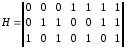(15 )

Количество
разрядов m
— определяет количество проверок.

В
первую проверку включают коэффициенты,
содержащие 1 в младшем (первом) разряде,
т. е. b₁,
b₃,
b₅
и т. д.

Во
вторую проверку включают коэффициенты,
содержащие 1 во втором разряде, т. е. b₂,
b₃,
b₆
и т. д.

В
третью проверку — коэффициенты которые
содержат 1 в третьем разряде и т. д.

Таблица
1

Для
обнаружения и исправления ошибки
составляются аналогичные проверки на
четность контрольных сумм, результатом
которых является двоичное (n-k)
-разрядное число, называемое синдромом
и указывающим на положение ошибки, т.
е. номер ошибочной позиции, который
определяется по двоичной записи числа,
либо по проверочной матрице.

Для
исправления ошибки необходимо
проинвертировать бит в ошибочной
позиции. Для исправления одиночной
ошибки и обнаружения двойной используют
дополнительную проверку на четность.
Если при исправлении ошибки контроль
на четность фиксирует ошибку, то значит
в кодовой комбинации две ошибки.

Схема
кодера и декодера для кода Хэмминга
приведена на рис. 1.

Пример
1.
Построить код Хемминга для передачи
сообщений в виде последовательности
десятичных цифр, представленных в виде
4 –х разрярных двоичных слов. Показать
процесс кодирования, декодирования и
исправления одиночной ошибки на примере
информационного слова 0101.

Решение:

1.
По заданной длине информационного слова
(k
= 4),
определим количество контрольных
разрядов m,
используя соотношение:

m
= [log₂
{(k+1)+
[log₂(k+1)]}]=[log₂
{(4+1)+
[log₂(4+1)]}]=3,

при
этом n
= k+m = 7,
т. е. получили (7, 4) -код.

2.
Определяем номера рабочих и контрольных
позиции кодовой комбинации. Номера
контрольных позиций выбираем по закону
2ⁱ
.

Для
рассматриваемой задачи (при n
= 7)
номера контрольных позиций равны 1, 2,
4. При этом кодовая комбинация имеет
вид:

b₁
b₂
b₃
b₄
b₅
b₆
b₇

к₁
к₂
0
к₃
1
0 1

3.
Определяем значения контрольных разрядов
(0 или 1), используя проверочную матрицу
(5).

Первая
проверка:

k₁

b₃
b₅
b₇
= k₁011
будет четной при k₁
=
0.

Вторая
проверка:

k₂

b₃
b₆
b₇
= k₂001
будет четной при k₂
=
1.

Третья
проверка:

k₃

b₅
b₆
b₇
= k₃101
будет четной при k₃
=
0.

1
2 3 4 5 6 7

Передаваемая
кодовая комбинация: 0 1 0 0 1 0 1

Допустим
принято: 0 1 1 0 1 0 1

Для
обнаружения и исправления ошибки
составим аналогичные про-верки на
четность контрольных сумм, в соответствии
с проверочной матрицей результатом
которых является двоичное (n-k)
-разрядное число, называемое синдромом
и указывающим на положение ошибки, т.
е, номер ошибочной позиции.

1)
k₁

b₃
b₅
b₇
= 0111 = 1.

2)
k₂

b₃
b₆
b₇
= 1101 = 1.

1. k₃
   
   b₅
   b₆
   b₇
   = 0101 = 0.

Сравнивая
синдром ошибки со столбцами проверочной
матрицы, определяем номер ошибочного
бита. Синдрому 011 соответствует третий
столбец, т. е. ошибка в третьем разряде
кодовой комбинации. Символ в 3 -й позиции
необходимо изменить на обратный.

Пример
2.
Построить код Хэмминга для передачи
кодовой комбинации 1 1 0 1 1 0 1 1. Показать
процесс обнаружения и исправления
ошибки в соответствующем разряде кодовой
комбинации.

Решение:
Рассмотрим
алгоритм построения кода для исправления
одиночной ошибки.

1.
По заданной длине информационного слова
(k
= 8)
, используя соотношения вычислим основные
параметры кода n
и m.

m
= [log₂
{(k+1)+
[log₂(k+1)]}]=[log₂
{(9+1)+
[log₂(9+1)]}]=4,

при
этом n
= k+m = 12,
т. е. получили (12, 8)-код.

2.
Определяем номера рабочих и контрольных
позиции кодовой комбинации. Номера
контрольных позиций выбираем по закону
2ⁱ
.

Для
рассматриваемой задачи (при n
= 12)
номера контрольных позиций равны 1, 4,
8.

При
этом кодовая комбинация имеет вид:

b₁
b₂
b₃
b₄
b₅
b₆
b₇
b₈
b₉
b₁₀
b₁₁
b₁₂

к₁
к₂
1
к₃
1
0 1 к₄
1
0 1 1

3.
Определяем значения контрольных разрядов
(0 или 1) путем много-кратных проверок
кодовой комбинации на четность. Количество
проверок равно m
= n-k.
В каждую проверку включается один
контрольный и определенные проверочные
биты.

Номера
информационных бит, включаемых в каждую
проверку определяется по двоичному
коду натуральных n-чисел
разрядностью — m.

0001
b₁
Количество разрядов m — определяет
количество прове-

0010
b₂
верок.

0011
b₃
1) к₁
b₃
b₅
b₇
b₉
а₁₁
=
к₁11111
=>

0100
b₄
четная
при к₁=1

0101
b₅
2)
к₂
b₃
b₆
b₇
b₁₀
b₁₁=
к₂10101
=>

0110
b₆
четная при к₂=1

0111
b₇
3)
к₃
b₅
b₆
b₇
b₁₂
=
к₃1011=>

1000
b₈
четная
при к₃=1

1001
b₉
4) к₄
b₉
b₁₀
b₁₁
b₁₂
=
к₁1011
=>

1010
b₁₀
четная
при к₄=1

1011
b₁₁

1100
b₁₂

Передаваемая
кодовая комбинация: 1 2 3 4 5 6 7 8 9 10 11 12

1
1 1 1 1 0 1 1 1 0 1 1

Допустим,
принято: 1 1 1 1 0 0 1 1 1 0 1 1

Для
обнаружения и исправления ошибки
составим аналогичные про-верки на
четность контрольных сумм, результатом
которых является двоичное (n-k)
-разрядное число, называемое синдромом
и указывающим на положение ошибки, т.
е. номер ошибочной позиции.

1)
к₁
b₃
b₅
b₇
b₉
b₁₁
=
110111 =1

2)
к₂
b₃
b₆
b₇
b₁₀
b₁₁
=
110101 =0

3)
к₃
b₅
b₆
b₇
b₁₂
=
10011 =1

4)
к₄
b₉
b₁₀
b₁₁
b₁₂
=
11011 =0

Обнаружена
ошибка в разряде кодовой комбинации с
номером 0101, т. е. в 5 -м разряде. Для
исправления ошибки необходимо
проинвертировать 5 -й разряд в кодовой
комбинации.

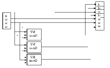
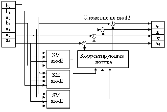
Рис.
1. Схема кодера —а
и декодера –б
для простого (7, 4) кода Хэмминга

Рассмотрим
применение кода Хэмминга. В ЭВМ код
Хэмминга чаще всего используется для
обнаружения и исправления ошибок в ОП,
памяти с обнаружением и исправлением
ошибок ECC Memory (Error Checking and Correcting). Код
Хэмминга используется как при параллельной,
так и при последовательной записи. В
ЭВМ значительная часть интенсивности
потока ошибок приходится на ОП. Причинами
постоянных неисправностей являются
отказы ИС, а случайных изменение
содержимого ОП за счет флуктуации
питающего напряжения, кратковременных
помех и излучений. Неисправность может
быть в одном бите, линии выборки разряда,
слова либо всей ИС. Сбой может возникнуть
при формировании кода (параллельного),
адреса или данных, поэтому защищать
необходимо и то и др. Обычно дешифратор
адреса встроен в м/схему и недоступен
для потребителя. Наиболее часто ошибки
дают ячейки памяти ЗУ, поэтому главным
образом защищают записываемые и
считываемые данные.

Наибольшее
применение в ЗУ нашли коды Хэмминга с
d_min=4,
исправляющие одиночные ошибки и
обнаруживающие двойные.

Проверочные
символы записываются либо в основное,
либо специальное ЗУ. Для каждого
записываемого информационного слова
(а не байта, как при контроле по паритету)
по определенным правилам вычисляется
функция свертки, результат которой
разрядностью в несколько бит также
записывается в память. Для 16 -ти разрядного
информационного слова используется 6
дополнительных бит (32- 7 бит, 64 –8 бит).
При считывании информации схема контроля,
используя избыточные биты, позволяет
обнаружить ошибки различной кратности
или исправить одиночную ошибку. Возможны
различные варианты поведения системы:

• автоматическое
  исправление ошибки без уведомления
  системы;

—
исправление однократной ошибки и
уведомление системы только о многократных
ошибках;

—
не исправление ошибки, а только уведомление
системы об ошибках;

Модуль
памяти со встроенной схемой исправления
ошибок –EOS 72/64 (ECC on Simm). Аналог микросхема
к 555 вж 1
-это 16 разрядная схема с обнаружением
и исправлением ошибок (ОИО) по коду
Хэмминга (22, 16), использование которой
позволяет исправить однократные ошибки
и обнаружить все двух кратные ошибки в
ЗУ.

Избыточные
(контрольные) разряды позволяют обнаружить
и исправить ошибки в ЗУ в процессе записи
и хранения информации.

В
составе ВЖ-1 используются 16 информационных
и 6 контрольных разрядов. (DB — информационное
слово, CB — контрольное слово).

При
записи осуществляется формирование
кода, состоящего из 16 информационных и
6 контрольных разрядов, представляющих
результат суммирование по модулю 2
восьми информационных разрядов в
соответствии с кодом Хэмминга.
Сформированные контрольные разряды
вместе с информационными поступают на
схему и записываются в ЗУ.

(22,16)

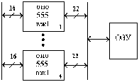
4
схе(72,64)

Рис.2.
Схема контроля

При
считывании шестнадцатиразрядное слово
декодируется, восстанавливаясь вместе
с 6 разрядным словом контрольным,
поступают на схему сравнения и контроля.
Если достигнуто равенство всех контрольных
разрядов и двоичных слов, то ошибки нет.

Любая
однократная ошибка в 16 разрядном слове
данных изменяет 3 байта в 6 разрядном
контрольном слове. Обнаруженный ошибочный
бит инвертируется.

Соседние файлы в предмете [НЕСОРТИРОВАННОЕ]

• #
• #
• #
• #
• #
• #
• #
• #
• #
• #
• #