Guidelines
Since the skewness and kurtosis of the normal distribution are zero, values for these two parameters should be close to zero for data to follow a normal distribution.
If the absolute value of the skewness for the data is more than twice the standard error this indicates that the data are not symmetric, and therefore not normal. Similarly, if the absolute value of the kurtosis for the data is more than twice the standard error this is also an indication that the data are not normal.
Example
Example 1: Use the above guidelines to gain more evidence as to whether the data in Example 1 of Graphical Tests for Normality and Symmetry are normally distributed.
As we can see from Graphical Tests for Normality and Symmetry, the skewness is SKEW(A4:A23) = .23 (cell D13) with standard error SQRT(6/COUNT(A4:A23)) = .55 (cell D16). Since .23 < 2*.55 = 1.10, the skewness is acceptable for a normal distribution. Also the kurtosis is KURT(A4:A23) = -1.53 (cell D14) with standard error of SQRT(24/COUNT(A4:A23)) = 1.10 (cell D17). Since 1.53 < 2*1.10 = 2.20, the kurtosis is also acceptable for a normal distribution.
Jarque-Barre Test
Related to the above approach is the Jarque-Barre (JB) test for normality which tests the null hypothesis that data from a sample of size n with skewness skew and kurtosis kurt. This test is based on the following property when the null hypothesis holds.
![]()
For Example 1
![]()
based on using the Excel worksheet functions SKEW and KURT to calculate the sample skewness and kurtosis values. Since CHISQ.DIST.RT(2.13, 2) = .345 > .05, we conclude there isn’t sufficient evidence to rule out the data coming from a normal population.
The JB test can also be performed using the population values of skewness and kurtosis, SKEWP (or SKEW.P) and KURTP functions (instead of SKEW and KURT).
![]()
Since CHISQ.DIST.RT(1.93, 2) = .382 > .05, once again we conclude there isn’t sufficient evidence to rule out the data coming from a normal population.
Worksheet Functions
Real Statistics Functions: The Real Statistics Resource Pack supplies the following functions.
JARQUE(R1, pop) = the Jarque-Barre test statistic JB for the data in the range R1
JBTEST(R1, pop) = p-value of the Jarque-Barre test on the data in R1
If pop = TRUE (default), the population version of the test is used; otherwise the sample version of the test is used. Any empty cells or cells containing non-numeric data are ignored.
For Example 1, we see that JARQUE(A4:A23) = 1.93 and JBTEST(A4:A23) = .382. Similarly, JARQUE(A4:A23, FALSE) = 2.13 and JBTEST(A4:A23, FALSE) = .345.
d’Agostino-Pearson Test
The d’Agostino-Pearson test of normality is also based on testing the skewness and kurtosis. This test is more accurate and so is more commonly used than the JB test. See D’Agostino-Pearson Test for details.
Reference
Wikipedia (2012) Jarque-Bera test
https://en.wikipedia.org/wiki/Jarque%E2%80%93Bera_test
The standard errors are valid for normal distributions, but not for other distributions. To see why, you can run the following code (which uses the spssSkewKurtosis function shown above) to estimate the true confidence level of the interval obtained by taking the kurtosis estimate plus or minus 1.96 standard errors:
set.seed(12345)
Nsim = 10000
Correct = numeric(Nsim)
b1.ols = numeric(Nsim)
b1.alt = numeric(Nsim)
for (i in 1:Nsim) {
 Data = rnorm(1000)
 Kurt = spssSkewKurtosis(Data)[2,1]
 seKurt =  spssSkewKurtosis(Data)[2,2]
  LowerLimit = Kurt -1.96*seKurt
  UpperLimit = Kurt +1.96*seKurt
  Correct[i] = LowerLimit <= 0 & 0 <= UpperLimit
 }

TrueConfLevel = mean(Correct)
TrueConfLevel
This gives you 0.9496, acceptably close to the expected 95%, so the standard errors work as expected when the data come from a normal distribution. But if you change Data = rnorm(1000) to Data = runif(1000), then you are assuming that the data come from a uniform distribution, whose theoretical (excess) kurtosis is -1.2. Making the corresponding change from Correct[i] = LowerLimit <= 0 & 0 <= UpperLimit to Correct[i] = LowerLimit <= -1.2 & -1.2 <= UpperLimit gives the result 1.0, meaning that the 95% intervals were always correct, rather than correct for 95% of the samples. Hence, the standard error seems to be overestimated (too large) for the (light-tailed) uniform distribution.
If you change Data = rnorm(1000) to Data = rexp(1000), then you are assuming that the data come from an exponential distribution, whose theoretical (excess) kurtosis is 6.0. Making the corresponding change from Correct[i] = LowerLimit <= 0 & 0 <= UpperLimit to Correct[i] = LowerLimit <= 6.0 & 6.0 <= UpperLimit gives the result 0.1007, meaning that the 95% intervals were correct only for 10.07% of the samples, rather than correct for 95% of the samples. Hence, the standard error seems to be underestimated (too small) for the (heavy-tailed) exponential distribution.
Those standard errors are grossly incorrect for non-normal distributions, as the simulation above shows. Thus, the only use of those standard errors is to compare the estimated kurtosis with the expected theoretical normal value (0.0); e.g., using a test of hypothesis. They cannot be used to construct a confidence interval for the true kurtosis.
- Kurtosis Examples
- Kurtosis Formulas
- Kurtosis or Excess Kurtosis?
- Kurtosis Calculation Example
- Platykurtic, Mesokurtic and Leptokurtic
In statistics, kurtosis refers to the “peakedness”
of the distribution for a quantitative variable.
What’s meant by “peakedness” is best understood from the example histograms shown below.
Kurtosis Examples
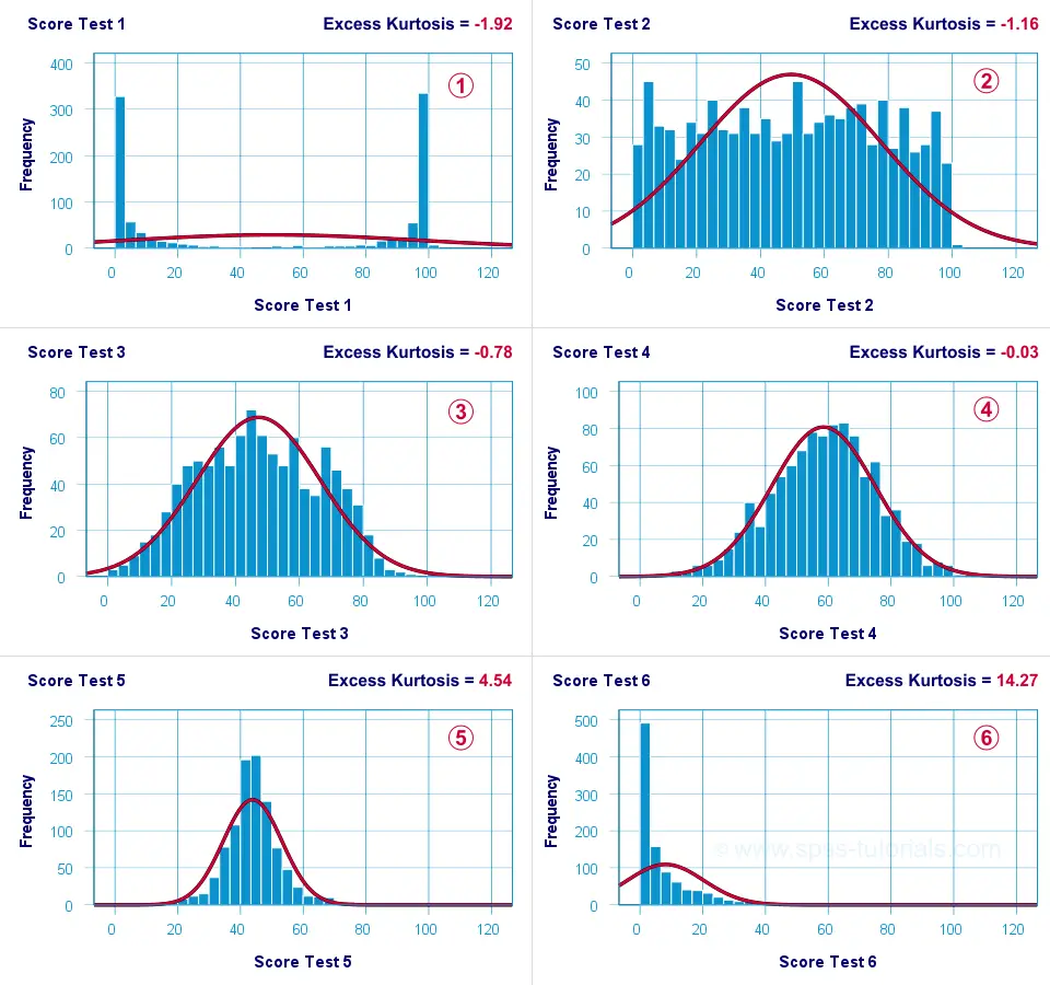
 Test 4 is almost perfectly normally distributed. Its excess kurtosis is therefore close to 0.
 The distribution for test 3 is somewhat “flatter” than the normal curve: the histogram bars are lower than the middle of the curve and higher towards its tails. Test 3 therefore has a negative excess kurtosis.
 Test 5 is more “peaked” than the normal curve: its bars are higher than the peak of the curve and lower towards its tails. Therefore, test 5 has a positive excess kurtosis.
 Test 2 roughly follows a uniform distribution. Because it’s even flatter than test 3, it has a stronger negative excess kurtosis.
 The strongest negative excess kurtosis is seen for test 1, which has a bimodal distribution.
 Positive excess kurtosis is often seen for variables having strong (positive) skewness such as test 6.
So now that we’ve an idea what (excess) kurtosis means, let’s see how it’s computed.
Kurtosis Formulas
If your data contain an entire population rather than just a sample, the population kurtosis (K_p) is computed as
$$K_p = frac{M_4}{M_2^2}$$
where (M_2) and (M_4) denote the second and fourth moments around the mean:
$$M_2 = frac{sumlimits_{i = 1}^N(X_i — overline{X})^2}{N}$$
and
$$M_4 = frac{sumlimits_{i = 1}^N(X_i — overline{X})^4}{N}$$
Note that (M_2) is simply the population-variance formula.
Kurtosis or Excess Kurtosis?
A normally distributed variable has a kurtosis of 3.0. Since this is undesirable, population excess kurtosis (EK_p) is defined as
$$EK_p = K_p — 3$$
so that excess kurtosis is 0.0 for a normally distributed variable.
Now, that’s all fine. But what’s not fine is that “kurtosis” refers to either kurtosis or excess kurtosis in standard textbooks and software packages without clarifying which of these two is reported.
Anyway.
Our formulas thus far only apply to data containing an entire population. If your data only contain a sample from some population -usually the case- then you’ll want to compute sample excess kurtosis (EK_s) as
$$EK_s = (N + 1) cdot EK_p + 6 cdot frac{(N — 1)}{(N — 2) cdot (N — 3)}$$
This formula results in “kurtosis” as reported by most software packages such as SPSS, Excel and Googlesheets. Finally, most text books suggest that the standard error for (excess) kurtosis (SE_{eks}) is computed as
$$SE_{eks} approx sqrt{frac{24}{N}}$$
This approximation, however, is not accurate for small sample sizes. Therefore, software packages use a more complicated formula. I won’t bother you with it.
Kurtosis Calculation Example
An example calculation for excess kurtosis is shown in this Googlesheet (read-only), partly shown below.
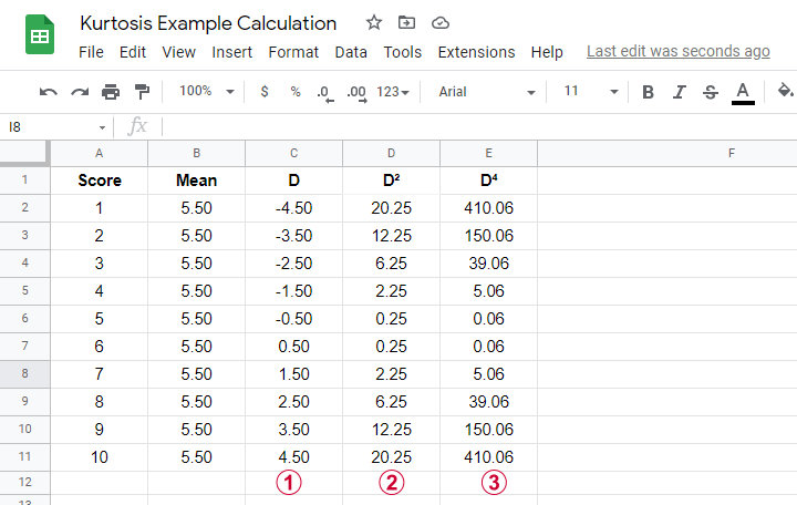
We computed excess kurtosis for scores 1 through 10. First off, we added their mean, M = 5.50. Next,
(D) denotes the difference scores (score — mean);
(D^2) are squared difference scores that are used for computing a variance;
(D^4) are difference scores raised to the fourth power.
As shown below, the remaining computations are fairly simple too.
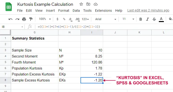
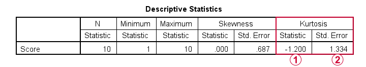
Note that the excess kurtosis = 1.20. The SPSS output shown below confirms this result.
Platykurtic, Mesokurtic & Leptokurtic
Some terminology related to excess kurtosis is that
- a variable having excess kurtosis < 0 is called platykurtic;
- a variable having excess kurtosis = 0 is called mesokurtic;
- a variable having excess kurtosis > 0 is called leptokurtic.
Our kurtosis examples illustrate what platykurtic, mesokurtic and leptokurtic distributions tend to look like.
Finding Kurtosis in Excel & SPSS
First off, “kurtosis” always refers to sample excess kurtosis in Excel, Googlesheets and SPSS. It’s found in Excel and Googlesheets by using something like
=KURT(A2:A11)
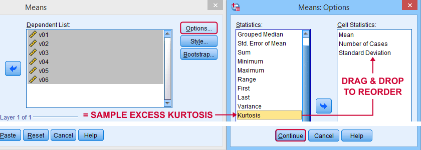
SPSS has many options for computing excess kurtosis but I personally prefer using
As shown below, kurtosis can be selected from Options and dragged into the desired position.
Right, I think that’s about it regarding (excess) kurtosis. If you’ve any questions or remarks, please throw me a comment below. Other than that:
thanks for reading!
In probability theory and statistics, kurtosis (from Greek: κυρτός, kyrtos or kurtos, meaning «curved, arching») is a measure of the «tailedness» of the probability distribution of a real-valued random variable. Like skewness, kurtosis describes a particular aspect of a probability distribution. There are different ways to quantify kurtosis for a theoretical distribution, and there are corresponding ways of estimating it using a sample from a population. Different measures of kurtosis may have different interpretations.
The standard measure of a distribution’s kurtosis, originating with Karl Pearson,[1] is a scaled version of the fourth moment of the distribution. This number is related to the tails of the distribution, not its peak;[2] hence, the sometimes-seen characterization of kurtosis as «peakedness» is incorrect. For this measure, higher kurtosis corresponds to greater extremity of deviations (or outliers), and not the configuration of data near the mean.
It is common to compare the excess kurtosis (defined below) of a distribution to 0, which is the excess kurtosis of any univariate normal distribution. Distributions with negative excess kurtosis are said to be platykurtic, although this does not imply the distribution is «flat-topped» as is sometimes stated. Rather, it means the distribution produces fewer and/or less extreme outliers than the normal distribution. An example of a platykurtic distribution is the uniform distribution, which does not produce outliers. Distributions with a positive excess kurtosis are said to be leptokurtic. An example of a leptokurtic distribution is the Laplace distribution, which has tails that asymptotically approach zero more slowly than a Gaussian, and therefore produces more outliers than the normal distribution. It is common practice to use excess kurtosis, which is defined as Pearson’s kurtosis minus 3, to provide a simple comparison to the normal distribution. Some authors and software packages use «kurtosis» by itself to refer to the excess kurtosis. For clarity and generality, however, this article explicitly indicates where non-excess kurtosis is meant.
Alternative measures of kurtosis are: the L-kurtosis, which is a scaled version of the fourth L-moment; measures based on four population or sample quantiles.[3] These are analogous to the alternative measures of skewness that are not based on ordinary moments.[3]
Pearson moments[edit]
The kurtosis is the fourth standardized moment, defined as
![{displaystyle operatorname {Kurt} [X]=operatorname {E} left[left({frac {X-mu }{sigma }}right)^{4}right]={frac {operatorname {E} left[(X-mu )^{4}right]}{left(operatorname {E} left[(X-mu )^{2}right]right)^{2}}}={frac {mu _{4}}{sigma ^{4}}},}](https://wikimedia.org/api/rest_v1/media/math/render/svg/abb6badbf13364972b05d9249962f5ff87aba236)
where μ4 is the fourth central moment and σ is the standard deviation. Several letters are used in the literature to denote the kurtosis. A very common choice is κ, which is fine as long as it is clear that it does not refer to a cumulant. Other choices include γ2, to be similar to the notation for skewness, although sometimes this is instead reserved for the excess kurtosis.
The kurtosis is bounded below by the squared skewness plus 1:[4]: 432

where μ3 is the third central moment. The lower bound is realized by the Bernoulli distribution. There is no upper limit to the kurtosis of a general probability distribution, and it may be infinite.
A reason why some authors favor the excess kurtosis is that cumulants are extensive. Formulas related to the extensive property are more naturally expressed in terms of the excess kurtosis. For example, let X1, …, Xn be independent random variables for which the fourth moment exists, and let Y be the random variable defined by the sum of the Xi. The excess kurtosis of Y is
![{displaystyle operatorname {Kurt} [Y]-3={frac {1}{left(sum _{j=1}^{n}sigma _{j}^{,2}right)^{2}}}sum _{i=1}^{n}sigma _{i}^{,4}cdot left(operatorname {Kurt} left[X_{i}right]-3right),}](https://wikimedia.org/api/rest_v1/media/math/render/svg/8f295e334581a6f264d3ca40bf75df3293fb0f3e)
where  is the standard deviation of
  . In particular if all of the Xi have the same variance, then this simplifies to
![{displaystyle operatorname {Kurt} [Y]-3={1 over n^{2}}sum _{i=1}^{n}left(operatorname {Kurt} left[X_{i}right]-3right).}](https://wikimedia.org/api/rest_v1/media/math/render/svg/6c397ae36f0e23dd0fff0c1137e5dcddc2e9217b)
The reason not to subtract 3 is that the bare fourth moment better generalizes to multivariate distributions, especially when independence is not assumed. The cokurtosis between pairs of variables is an order four tensor. For a bivariate normal distribution, the cokurtosis tensor has off-diagonal terms that are neither 0 nor 3 in general, so attempting to «correct» for an excess becomes confusing. It is true, however, that the joint cumulants of degree greater than two for any multivariate normal distribution are zero.
For two random variables, X and Y, not necessarily independent, the kurtosis of the sum, X + Y, is
![{displaystyle {begin{aligned}operatorname {Kurt} [X+Y]={1 over sigma _{X+Y}^{4}}{big (}&sigma _{X}^{4}operatorname {Kurt} [X]+4sigma _{X}^{3}sigma _{Y}operatorname {Cokurt} [X,X,X,Y]\&{}+6sigma _{X}^{2}sigma _{Y}^{2}operatorname {Cokurt} [X,X,Y,Y]\[6pt]&{}+4sigma _{X}sigma _{Y}^{3}operatorname {Cokurt} [X,Y,Y,Y]+sigma _{Y}^{4}operatorname {Kurt} [Y]{big )}.end{aligned}}}](https://wikimedia.org/api/rest_v1/media/math/render/svg/ca0a7f4889310fb96ed071c23a6d6af959ef500d)
Note that the fourth-power binomial coefficients (1, 4, 6, 4, 1) appear in the above equation.
Interpretation[edit]
The exact interpretation of the Pearson measure of kurtosis (or excess kurtosis) used to be disputed, but is now settled. As Westfall notes in 2014[2], «…its only unambiguous interpretation is in terms of tail extremity; i.e., either existing outliers (for the sample kurtosis) or propensity to produce outliers (for the kurtosis of a probability distribution).» The logic is simple: Kurtosis is the average (or expected value) of the standardized data raised to the fourth power. Standardized values that are less than 1 (i.e., data within one standard deviation of the mean, where the «peak» would be) contribute virtually nothing to kurtosis, since raising a number that is less than 1 to the fourth power makes it closer to zero. The only data values (observed or observable) that contribute to kurtosis in any meaningful way are those outside the region of the peak; i.e., the outliers. Therefore, kurtosis measures outliers only; it measures nothing about the «peak».
Many incorrect interpretations of kurtosis that involve notions of peakedness have been given. One is that kurtosis measures both the «peakedness» of the distribution and the heaviness of its tail.[5] Various other incorrect interpretations have been suggested, such as «lack of shoulders» (where the «shoulder» is defined vaguely as the area between the peak and the tail, or more specifically as the area about one standard deviation from the mean) or «bimodality».[6] Balanda and MacGillivray assert that the standard definition of kurtosis «is a poor measure of the kurtosis, peakedness, or tail weight of a distribution»[5]: 114 and instead propose to «define kurtosis vaguely as the location- and scale-free movement of probability mass from the shoulders of a distribution into its center and tails».[5]
Moors’ interpretation[edit]
In 1986 Moors gave an interpretation of kurtosis.[7] Let

where X is a random variable, μ is the mean and σ is the standard deviation.
Now by definition of the kurtosis  , and by the well-known identity
 ![{displaystyle Eleft[V^{2}right]=operatorname {var} [V]+[E[V]]^{2},}](https://wikimedia.org/api/rest_v1/media/math/render/svg/6782f578cb9d22c509a08ab7d43a21735eba1cde)
![{displaystyle kappa =Eleft[Z^{4}right]=operatorname {var} left[Z^{2}right]+left[Eleft[Z^{2}right]right]^{2}=operatorname {var} left[Z^{2}right]+[operatorname {var} [Z]]^{2}=operatorname {var} left[Z^{2}right]+1}](data:image/svg+xml,%3Csvg%20xmlns='http://www.w3.org/2000/svg'%20viewBox='0%200%200%200'%3E%3C/svg%3E) .
.
![{displaystyle kappa =Eleft[Z^{4}right]=operatorname {var} left[Z^{2}right]+left[Eleft[Z^{2}right]right]^{2}=operatorname {var} left[Z^{2}right]+[operatorname {var} [Z]]^{2}=operatorname {var} left[Z^{2}right]+1}](https://wikimedia.org/api/rest_v1/media/math/render/svg/8ed2d37d4494e13b10f81b83797c0d689ff740d2)
The kurtosis can now be seen as a measure of the dispersion of Z2 around its expectation. Alternatively it can be seen to be a measure of the dispersion of Z around +1 and −1. κ attains its minimal value in a symmetric two-point distribution. In terms of the original variable X, the kurtosis is a measure of the dispersion of X around the two values μ ± σ.
High values of κ arise in two circumstances:
- where the probability mass is concentrated around the mean and the data-generating process produces occasional values far from the mean,
- where the probability mass is concentrated in the tails of the distribution.
Excess kurtosis[edit]
The excess kurtosis is defined as kurtosis minus 3. There are 3 distinct regimes as described below.
Mesokurtic[edit]
Distributions with zero excess kurtosis are called mesokurtic, or mesokurtotic. The most prominent example of a mesokurtic distribution is the normal distribution family, regardless of the values of its parameters. A few other well-known distributions can be mesokurtic, depending on parameter values: for example, the binomial distribution is mesokurtic for  .
.
Leptokurtic[edit]
A distribution with positive excess kurtosis is called leptokurtic, or leptokurtotic. «Lepto-» means «slender».[8] In terms of shape, a leptokurtic distribution has fatter tails. Examples of leptokurtic distributions include the Student’s t-distribution, Rayleigh distribution, Laplace distribution, exponential distribution, Poisson distribution and the logistic distribution. Such distributions are sometimes termed super-Gaussian.[9]
Platykurtic[edit]

The coin toss is the most platykurtic distribution
A distribution with negative excess kurtosis is called platykurtic, or platykurtotic. «Platy-» means «broad».[10] In terms of shape, a platykurtic distribution has thinner tails. Examples of platykurtic distributions include the continuous and discrete uniform distributions, and the raised cosine distribution. The most platykurtic distribution of all is the Bernoulli distribution with p = 1/2 (for example the number of times one obtains «heads» when flipping a coin once, a coin toss), for which the excess kurtosis is −2.
Graphical examples[edit]
The Pearson type VII family[edit]

pdf for the Pearson type VII distribution with excess kurtosis of infinity (red); 2 (blue); and 0 (black)

log-pdf for the Pearson type VII distribution with excess kurtosis of infinity (red); 2 (blue); 1, 1/2, 1/4, 1/8, and 1/16 (gray); and 0 (black)
The effects of kurtosis are illustrated using a parametric family of distributions whose kurtosis can be adjusted while their lower-order moments and cumulants remain constant. Consider the Pearson type VII family, which is a special case of the Pearson type IV family restricted to symmetric densities. The probability density function is given by
![f(x; a, m) = frac{Gamma(m)}{a,sqrt{pi},Gamma(m-1/2)} left[1+left(frac{x}{a}right)^2 right]^{-m}, !](https://wikimedia.org/api/rest_v1/media/math/render/svg/688a4a90b74edb0216f35dd7fd915132f37599f8)
where a is a scale parameter and m is a shape parameter.
All densities in this family are symmetric. The kth moment exists provided m > (k + 1)/2. For the kurtosis to exist, we require m > 5/2. Then the mean and skewness exist and are both identically zero. Setting a2 = 2m − 3 makes the variance equal to unity. Then the only free parameter is m, which controls the fourth moment (and cumulant) and hence the kurtosis. One can reparameterize with  , where
  is the excess kurtosis as defined above. This yields a one-parameter leptokurtic family with zero mean, unit variance, zero skewness, and arbitrary non-negative excess kurtosis. The reparameterized density is

In the limit as  one obtains the density

which is shown as the red curve in the images on the right.
In the other direction as  one obtains the standard normal density as the limiting distribution, shown as the black curve.
In the images on the right, the blue curve represents the density  with excess kurtosis of 2. The top image shows that leptokurtic densities in this family have a higher peak than the mesokurtic normal density, although this conclusion is only valid for this select family of distributions. The comparatively fatter tails of the leptokurtic densities are illustrated in the second image, which plots the natural logarithm of the Pearson type VII densities: the black curve is the logarithm of the standard normal density, which is a parabola. One can see that the normal density allocates little probability mass to the regions far from the mean («has thin tails»), compared with the blue curve of the leptokurtic Pearson type VII density with excess kurtosis of 2. Between the blue curve and the black are other Pearson type VII densities with γ2 = 1, 1/2, 1/4, 1/8, and 1/16. The red curve again shows the upper limit of the Pearson type VII family, with
  (which, strictly speaking, means that the fourth moment does not exist). The red curve decreases the slowest as one moves outward from the origin («has fat tails»).
Other well-known distributions[edit]
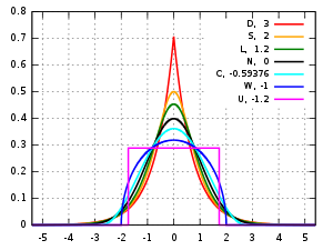

Several well-known, unimodal, and symmetric distributions from different parametric families are compared here. Each has a mean and skewness of zero. The parameters have been chosen to result in a variance equal to 1 in each case. The images on the right show curves for the following seven densities, on a linear scale and logarithmic scale:
- D: Laplace distribution, also known as the double exponential distribution, red curve (two straight lines in the log-scale plot), excess kurtosis = 3
- S: hyperbolic secant distribution, orange curve, excess kurtosis = 2
- L: logistic distribution, green curve, excess kurtosis = 1.2
- N: normal distribution, black curve (inverted parabola in the log-scale plot), excess kurtosis = 0
- C: raised cosine distribution, cyan curve, excess kurtosis = −0.593762…
- W: Wigner semicircle distribution, blue curve, excess kurtosis = −1
- U: uniform distribution, magenta curve (shown for clarity as a rectangle in both images), excess kurtosis = −1.2.
Note that in these cases the platykurtic densities have bounded support, whereas the densities with positive or zero excess kurtosis are supported on the whole real line.
One cannot infer that high or low kurtosis distributions have the characteristics indicated by these examples. There exist platykurtic densities with infinite support,
- e.g., exponential power distributions with sufficiently large shape parameter b
and there exist leptokurtic densities with finite support.
- e.g., a distribution that is uniform between −3 and −0.3, between −0.3 and 0.3, and between 0.3 and 3, with the same density in the (−3, −0.3) and (0.3, 3) intervals, but with 20 times more density in the (−0.3, 0.3) interval
Also, there exist platykurtic densities with infinite peakedness,
- e.g., an equal mixture of the beta distribution with parameters 0.5 and 1 with its reflection about 0.0
and there exist leptokurtic densities that appear flat-topped,
- e.g., a mixture of distribution that is uniform between -1 and 1 with a T(4.0000001) Student’s t-distribution, with mixing probabilities 0.999 and 0.001.
Sample kurtosis[edit]
Definitions[edit]
A natural but biased estimator[edit]
For a sample of n values, a method of moments estimator of the population excess kurtosis can be defined as
![{displaystyle g_{2}={frac {m_{4}}{m_{2}^{2}}}-3={frac {{tfrac {1}{n}}sum _{i=1}^{n}(x_{i}-{overline {x}})^{4}}{left[{tfrac {1}{n}}sum _{i=1}^{n}(x_{i}-{overline {x}})^{2}right]^{2}}}-3}](https://wikimedia.org/api/rest_v1/media/math/render/svg/e30ed8db4466ff3e448b71e729464506ddce7770)
where m4 is the fourth sample moment about the mean, m2 is the second sample moment about the mean (that is, the sample variance), xi is the ith value, and  is the sample mean.
This formula has the simpler representation,

where the  values are the standardized data values using the standard deviation defined using n rather than n − 1 in the denominator.
For example, suppose the data values are 0, 3, 4, 1, 2, 3, 0, 2, 1, 3, 2, 0, 2, 2, 3, 2, 5, 2, 3, 999.
Then the values are −0.239, −0.225, −0.221, −0.234, −0.230, −0.225, −0.239, −0.230, −0.234, −0.225, −0.230, −0.239, −0.230, −0.230, −0.225, −0.230, −0.216, −0.230, −0.225, 4.359
and the  values are 0.003, 0.003, 0.002, 0.003, 0.003, 0.003, 0.003, 0.003, 0.003, 0.003, 0.003, 0.003, 0.003, 0.003, 0.003, 0.003, 0.002, 0.003, 0.003, 360.976.
The average of these values is 18.05 and the excess kurtosis is thus 18.05 − 3 = 15.05. This example makes it clear that data near the «middle» or «peak» of the distribution do not contribute to the kurtosis statistic, hence kurtosis does not measure «peakedness». It is simply a measure of the outlier, 999 in this example.
Standard unbiased estimator[edit]
Given a sub-set of samples from a population, the sample excess kurtosis  above is a biased estimator of the population excess kurtosis. An alternative estimator of the population excess kurtosis, which is unbiased in random samples of a normal distribution, is defined as follows:[3]
![{displaystyle {begin{aligned}G_{2}&={frac {k_{4}}{k_{2}^{2}}}\[6pt]&={frac {n^{2},[(n+1),m_{4}-3,(n-1),m_{2}^{2}]}{(n-1),(n-2),(n-3)}};{frac {(n-1)^{2}}{n^{2},m_{2}^{2}}}\[6pt]&={frac {n-1}{(n-2),(n-3)}}left[(n+1),{frac {m_{4}}{m_{2}^{2}}}-3,(n-1)right]\[6pt]&={frac {n-1}{(n-2),(n-3)}}left[(n+1),g_{2}+6right]\[6pt]&={frac {(n+1),n,(n-1)}{(n-2),(n-3)}};{frac {sum _{i=1}^{n}(x_{i}-{bar {x}})^{4}}{left(sum _{i=1}^{n}(x_{i}-{bar {x}})^{2}right)^{2}}}-3,{frac {(n-1)^{2}}{(n-2),(n-3)}}\[6pt]&={frac {(n+1),n}{(n-1),(n-2),(n-3)}};{frac {sum _{i=1}^{n}(x_{i}-{bar {x}})^{4}}{k_{2}^{2}}}-3,{frac {(n-1)^{2}}{(n-2)(n-3)}}end{aligned}}}](https://wikimedia.org/api/rest_v1/media/math/render/svg/51b0b3b5d766ffd8f2c3be0fbe899873b41bb961)
where k4 is the unique symmetric unbiased estimator of the fourth cumulant, k2 is the unbiased estimate of the second cumulant (identical to the unbiased estimate of the sample variance), m4 is the fourth sample moment about the mean, m2 is the second sample moment about the mean, xi is the ith value, and  is the sample mean. This adjusted Fisher–Pearson standardized moment coefficient
  is the version found in Excel and several statistical packages including Minitab, SAS, and SPSS.[11]
Unfortunately, in nonnormal samples is itself generally biased.
Upper bound[edit]
An upper bound for the sample kurtosis of n (n > 2) real numbers is[12]

where  is the corresponding sample skewness.
Variance under normality[edit]
The variance of the sample kurtosis of a sample of size n from the normal distribution is[13]

Stated differently, under the assumption that the underlying random variable  is normally distributed, it can be shown that
  .[14]: Page number needed
Applications[edit]
|
This section needs expansion. You can help by adding to it. (December 2009) |
The sample kurtosis is a useful measure of whether there is a problem with outliers in a data set. Larger kurtosis indicates a more serious outlier problem, and may lead the researcher to choose alternative statistical methods.
D’Agostino’s K-squared test is a goodness-of-fit normality test based on a combination of the sample skewness and sample kurtosis, as is the Jarque–Bera test for normality.
For non-normal samples, the variance of the sample variance depends on the kurtosis; for details, please see variance.
Pearson’s definition of kurtosis is used as an indicator of intermittency in turbulence.[15] It is also used in magnetic resonance imaging to quantify non-Gaussian diffusion.[16]
A concrete example is the following lemma by He, Zhang, and Zhang:[17]
Assume a random variable has expectation ![{displaystyle E[X]=mu }](https://wikimedia.org/api/rest_v1/media/math/render/svg/51ed977b56d8e513d9eb92193de5454ac545231e) , variance
, variance ![{displaystyle Eleft[(X-mu )^{2}right]=sigma ^{2}}](https://wikimedia.org/api/rest_v1/media/math/render/svg/cedd17629b1a84a72ee82ac046028e7628811148) and kurtosis
and kurtosis ![{displaystyle kappa ={tfrac {1}{sigma ^{4}}}Eleft[(X-mu )^{4}right]}](https://wikimedia.org/api/rest_v1/media/math/render/svg/f9596b45af565b781abac4f4bad3ae95dc48f57f) .
.
Assume we sample  many independent copies. Then
- .
![{displaystyle Pr left[max _{i=1}^{n}X_{i}leq mu right]leq delta quad {text{and}}quad Pr left[min _{i=1}^{n}X_{i}geq mu right]leq delta }](https://wikimedia.org/api/rest_v1/media/math/render/svg/7dd308935ef5c101697f8d1f64b76d7e42591ad6)
This shows that with  many samples, we will see one that is above the expectation with probability at least
  .
.
In other words: If the kurtosis is large, we might see a lot values either all below or above the mean.
Kurtosis convergence[edit]
Applying band-pass filters to digital images, kurtosis values tend to be uniform, independent of the range of the filter. This behavior, termed kurtosis convergence, can be used to detect image splicing in forensic analysis.[18]
Other measures[edit]
A different measure of «kurtosis» is provided by using L-moments instead of the ordinary moments.[19][20]
See also[edit]
![]()
Wikimedia Commons has media related to Kurtosis.
- Kurtosis risk
- Maximum entropy probability distribution
References[edit]
- ^
Pearson, Karl (1905), «Das Fehlergesetz und seine Verallgemeinerungen durch Fechner und Pearson. A Rejoinder» [The Error Law and its Generalizations by Fechner and Pearson. A Rejoinder], Biometrika, 4 (1–2): 169–212, doi:10.1093/biomet/4.1-2.169, JSTOR 2331536 - ^ a b
Westfall, Peter H. (2014), «Kurtosis as Peakedness, 1905 — 2014. R.I.P.«, The American Statistician, 68 (3): 191–195, doi:10.1080/00031305.2014.917055, PMC 4321753, PMID 25678714 - ^ a b c
Joanes, Derrick N.; Gill, Christine A. (1998), «Comparing measures of sample skewness and kurtosis», Journal of the Royal Statistical Society, Series D, 47 (1): 183–189, doi:10.1111/1467-9884.00122, JSTOR 2988433 - ^
Pearson, Karl (1916), «Mathematical Contributions to the Theory of Evolution. — XIX. Second Supplement to a Memoir on Skew Variation.», Philosophical Transactions of the Royal Society of London A, 216 (546): 429–457, Bibcode:1916RSPTA.216..429P, doi:10.1098/rsta.1916.0009, JSTOR 91092 - ^ a b c
Balanda, Kevin P.; MacGillivray, Helen L. (1988), «Kurtosis: A Critical Review», The American Statistician, 42 (2): 111–119, doi:10.2307/2684482, JSTOR 2684482 - ^
Darlington, Richard B. (1970), «Is Kurtosis Really ‘Peakedness’?», The American Statistician, 24 (2): 19–22, doi:10.1080/00031305.1970.10478885, JSTOR 2681925 - ^
Moors, J. J. A. (1986), «The meaning of kurtosis: Darlington reexamined», The American Statistician, 40 (4): 283–284, doi:10.1080/00031305.1986.10475415, JSTOR 2684603 - ^ «Lepto-«.
- ^
Benveniste, Albert; Goursat, Maurice; Ruget, Gabriel (1980), «Robust identification of a nonminimum phase system: Blind adjustment of a linear equalizer in data communications», IEEE Transactions on Automatic Control, 25 (3): 385–399, doi:10.1109/tac.1980.1102343 - ^ «platy-: definition, usage and pronunciation — YourDictionary.com». Archived from the original on 2007-10-20.
- ^ Doane DP, Seward LE (2011) J Stat Educ 19 (2)
- ^
Sharma, Rajesh; Bhandari, Rajeev K. (2015), «Skewness, kurtosis and Newton’s inequality», Rocky Mountain Journal of Mathematics, 45 (5): 1639–1643, doi:10.1216/RMJ-2015-45-5-1639, S2CID 88513237 - ^
Fisher, Ronald A. (1930), «The Moments of the Distribution for Normal Samples of Measures of Departure from Normality», Proceedings of the Royal Society A, 130 (812): 16–28, Bibcode:1930RSPSA.130…16F, doi:10.1098/rspa.1930.0185, JSTOR 95586, S2CID 121520301 - ^
Kendall, Maurice G.; Stuart, Alan (1969), The Advanced Theory of Statistics, Volume 1: Distribution Theory (3rd ed.), London, UK: Charles Griffin & Company Limited, ISBN 0-85264-141-9 - ^
Sandborn, Virgil A. (1959), «Measurements of Intermittency of Turbulent Motion in a Boundary Layer», Journal of Fluid Mechanics, 6 (2): 221–240, Bibcode:1959JFM…..6..221S, doi:10.1017/S0022112059000581, S2CID 121838685 - ^ Jensen, J.; Helpern, J.; Ramani, A.; Lu, H.; Kaczynski, K. (19 May 2005). «Diffusional kurtosis imaging: The quantification of non‐Gaussian water diffusion by means of magnetic resonance imaging». Magn Reson Med. 53 (6): 1432–1440. doi:10.1002/mrm.20508. PMID 15906300. S2CID 11865594.
- ^ He, S.; Zhang, J.; Zhang, S. (2010). «Bounding probability of small deviation: A fourth moment approach». Mathematics of Operations Research. 35 (1): 208–232. doi:10.1287/moor.1090.0438. S2CID 11298475.
- ^
Pan, Xunyu; Zhang, Xing; Lyu, Siwei (2012), «Exposing Image Splicing with Inconsistent Local Noise Variances», 2012 IEEE International Conference on Computational Photography (ICCP), 28-29 April 2012; Seattle, WA, USA: IEEE, doi:10.1109/ICCPhot.2012.6215223, S2CID 14386924{{citation}}: CS1 maint: location (link) - ^
Hosking, Jonathan R. M. (1992), «Moments or L moments? An example comparing two measures of distributional shape», The American Statistician, 46 (3): 186–189, doi:10.1080/00031305.1992.10475880, JSTOR 2685210 - ^
Hosking, Jonathan R. M. (2006), «On the characterization of distributions by their L-moments», Journal of Statistical Planning and Inference, 136 (1): 193–198, doi:10.1016/j.jspi.2004.06.004
Further reading[edit]
- Kim, Tae-Hwan; White, Halbert (2003). «On More Robust Estimation of Skewness and Kurtosis: Simulation and Application to the S&P500 Index». Finance Research Letters. 1: 56–70. doi:10.1016/S1544-6123(03)00003-5. S2CID 16913409. Alternative source (Comparison of kurtosis estimators)
- Seier, E.; Bonett, D.G. (2003). «Two families of kurtosis measures». Metrika. 58: 59–70. doi:10.1007/s001840200223. S2CID 115990880.
External links[edit]
![]()
Wikiversity has learning resources about Kurtosis
- «Excess coefficient», Encyclopedia of Mathematics, EMS Press, 2001 [1994]
- Kurtosis calculator
- Free Online Software (Calculator) computes various types of skewness and kurtosis statistics for any dataset (includes small and large sample tests)..
- Kurtosis on the Earliest known uses of some of the words of mathematics
- Celebrating 100 years of Kurtosis a history of the topic, with different measures of kurtosis.
Mean — средняя
арифметическая;
Среднее значение
случайной величины представляет собой
наиболее типичное, наиболее вероятное
ее значение, своеобразный центр, вокруг
которого разбросаны все значения
признака.
Sum — сумма;
Median — медиана;
Медианой является
такое значение случайной величины,
которое разделяет все случаи выборки
на две равные по численности части.
Standard Deviation
— стандартное отклонение;
Стандартное
отклонение (или среднее квадратическое
отклонение) является мерой изменчивости
(вариации) признака. Оно показывает на
какую величину в среднем отклоняются
случаи от среднего значения признака.
Особенно большое значение имеет при
исследовании нормальных распределений.
В нормальном распределении 68% всех
случаев лежит в интервале +
одного отклонения от среднего, 95% — +
двух стандартных отклонений от среднего
и 99,7% всех случаев — в интервале +
трех стандартных отклонений от среднего.
V Рис. 8. Окно выбора статистик ariance — дисперсия;
Дисперсия является
мерой изменчивости, вариации признака
и представляет собой средний квадрат
отклонений случаев от среднего значения
признака. В отличии от других показателей
вариации дисперсия может быть разложена
на составные части, что позволяет тем
самым оценить влияние различных факторов
на вариацию признака. Дисперсия — один
из существеннейших показателей,
характеризующих явление или процесс,
один из основных критериев возможности
создания достаточно точных моделей.
Standard error of mean
— стандартная ошибка
среднего;
Стандартная ошибка
среднего это величина, на которую
отличается среднее значение выборки
от среднего значения генеральной
совокупности при условии, что распределение
близко к нормальному. С вероятностью
0,68 можно утверждать, что среднее значение
генеральной совокупности лежит в
интервале +
одной стандартной ошибки от среднего,
с вероятностью 0,95 — в интервале +
двух стандартных ошибок от среднего и
с вероятностью 0,99 — среднее значение
генеральной совокупности лежит в
интервале +
трех стандартных ошибок от среднего.
95% Confidence limits of mean — 95%-ый доверительный интервал для среднего;
Интервал, в который
с вероятностью 0,95 попадает среднее
значение признака генеральной
совокупности.
Minimum, maximum
— минимальное и максимальное значения;
Lower, upper
quartiles — нижний
и верхний квартили;
Верхний квартиль
это такое значение случайной величины,
больше которого по величине 25% случаев
выборки. Верхний квартиль это такое
значение случайной величины, меньше
которого по величине 25% случаев выборки.
Range — размах;
Расстояние между
наибольшим (maximum)
и наименьшим (minimum)
значениями признака.
Quartile range
— интерквартильная широта;
Расстояние между
нижним и верхним квартилями.
Skewness -асимметрия;
Асимметрия
характеризует степень смещения
вариационного ряда относительно среднего
значения по величине и направлению. В
симметричной кривой коэффициент
асимметрии равен нулю. Если правая ветвь
кривой, начиная от вершины) больше левой
(правосторонняя асимметрия), то коэффициент
асимметрии больше нуля. Если левая ветвь
кривой больше правой (левосторонняя
асимметрия), то коэффициент асимметрии
меньше нуля. Асимметрия менее 0,5 считается
малой.
Standard error
of Skewness
-стандартная ошибка асимметрии;
Kurtosis — эксцесс;
Эксцесс характеризует
степень концентрации случаев вокруг
среднего значения и является своеобразной
мерой крутости кривой. В кривой нормального
распределения эксцесс равен нулю. Если
эксцесс больше нуля, то кривая распределения
характеризуется островершинностью,
т.е. является более крутой по сравнению
с нормальной, а случаи более густо
группируются вокруг среднего. При
отрицательном эксцессе кривая является
более плосковершинной, т.е. более пологой
по сравнению с нормальным распределением.
Отрицательным пределом величины эксцесса
является число -2, положительного предела
— нет.
Standard error
of Kurtosis
— стандартная ошибка эксцесса.
На против статистик, подлежащих вычислению
(рис.  следует поставить флажок.
После нажатия на кнопку OK
окна Descriptive statistics
на экране появится таблица с результатами
расчетов описательных статистик (рис.
9).
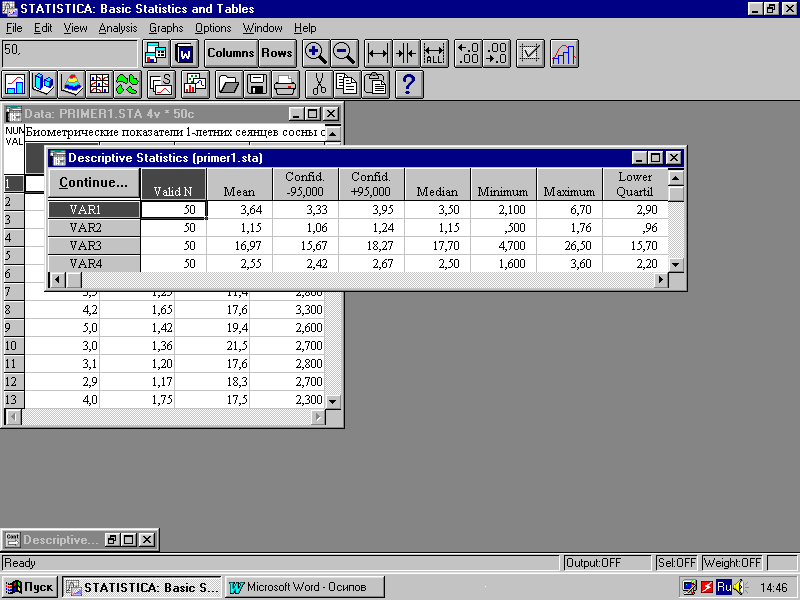
Рис. 9. Окно с результатами расчета
описательных статистик
В таблице 2 эти данные представлены
после копирования в текстовый редактор
Word.
К сожалению, пакет Statistica
не рассчитывает такие часто применяемые
статистики, как коэффициент вариации
и относительная ошибка среднего значения
(точность опыта). Но их определение не
представляет большого труда. Коэффициент
вариации (%) есть отношение стандартного
отклонения к среднему значению, умноженное
на 100%:
![]()
Коэффициент
вариации, как дисперсия и стандартное
отклонение, является показателем
изменчивости признака. Коэффициент
вариации не зависит от единиц измерения,
поэтому удобен для сравнительной оценки
различных статистических совокупностей.
При величине коэффициента вариации до
10% изменчивость оценивается как слабая,
11-25% — средняя, более 25% — сильная (Лакин,
1990).
О![]()
тносительная
ошибка среднего значения (%) — отношение
стандартной ошибки среднего к среднему
значению, умноженное на 100% (для вероятности
0,68):
Это процент
расхождения между генеральной и
выборочной средней, показывает на
сколько процентов можно ошибиться, если
утверждать, что генеральная средняя
равна выборочной средней. Если
относительная ошибка не превышает 5%,
то точность исследований (точность
опыта) оценивается как хорошая, до 10% —
удовлетворительная.
Точность 3-5% при
вероятности 0,95, а в некоторых случаях
и при вероятности 0,68, является вполне
достаточной для большинства задач
лесного хозяйства.
П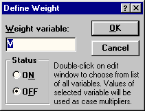
Рис.106. Окно задания
переменной- весов
ри необходимости обработки
сгруппированных данных нужно
воспользоваться кнопкой Weight
окна Descriptive statistics
(рис.4). В появляющемся диалоговом окне
(рис. 10) следует указать переменную,
являющуюся весами для других переменных
(Weight variables),
а переключатель Status
установить в положение ON.
Необходимо иметь в виду, что весы
действуют сразу для всех переменных.
Поэтому обрабатывать сгруппированные
и не сгруппированные данные нужно
отдельно.
При помощи опции Alpha
error (рис. 4)
выбирается уровень доверительной
вероятности статистического анализа.
В биологических исследованиях наиболее
часто используется вероятность 0,95
(95%). Вероятности 0,95 соответствует уровень
значимости 0,05 (5%).
Кнопка Select cases
позволяет установить условия включения
(include if) или
исключения (exclude if)
случаев (строк файла данных) из
статистической обработки (рис. 11).
Операторы, которые могут использоваться
при написании выражений, а также примеры
самих выражений имеются непосредственно
на самом диалоговом окне Case
Selection Conditions
(рис. 11) в нижней его части.
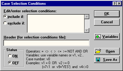
Рис. 11. Окно задания условий выбора
случаев
Для визуализации описательных статистик
можно построить статистические графики
типа «коробок» (или «ящиков с
усами»). Это легко можно сделать при
помощи кнопки Box &
Whisker plot
for all
variable окна Descriptive
statistics. На графике можно
отобразить 3 статистики, установив
переключатель в одно из 4-х положений
(рис. 12):
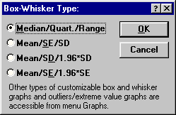
Рис. 12. Окно выбора статистик для
графика коробок
-
Median/Quart./Range
— Медиана / Квартили / Размах; -
Mean/SE/SD
— Среднее / Ошибка среднего / Стандартное
отклонение -
Mean/SD/1.96SD
— Среднее / Стандартное отклонение /
Интервал 1,96* стандартного отклонения; -
Mean/SE/1.96*SE
— Среднее / Ошибка среднего / Интервал
1,96 * ошибки среднего.
В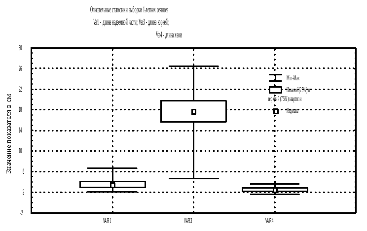
изуализация
описательных статистик переменных
VAR1, VAR3 и
VAR4 рассматриваемого
примера при помощи графика коробок
представлена на рис. 13.
Рис. 13. Описательные статистики в
графическом виде
Соседние файлы в папке Статистика
- #
- #
- #
- #
- #
- #
- #
- #
- #
- #
And a guide to using the Omnibus K-squared and Jarque–Bera normality tests
We’ll cover the following four topics in this section:
- What is normality and why should you care if the residual errors from your trained regression model are normally distributed?
- What are Skewness and Kurtosis measures and how to use them for testing for normality of residual errors?
- How to use two very commonly used tests of normality, namely the Omnibus K-squared and Jarque–Bera tests that are based on Skewness and Kurtosis.
- How to apply these tests to a real-world data set to decide if Ordinary Least Squares regression is the appropriate model for this data set.
What is normality?
Normality means that your data follows the normal distribution. Specifically, each value y_i in Y is a ‘realization’ of some normally distributed random variable N(µ_i, σ_i) as follows:
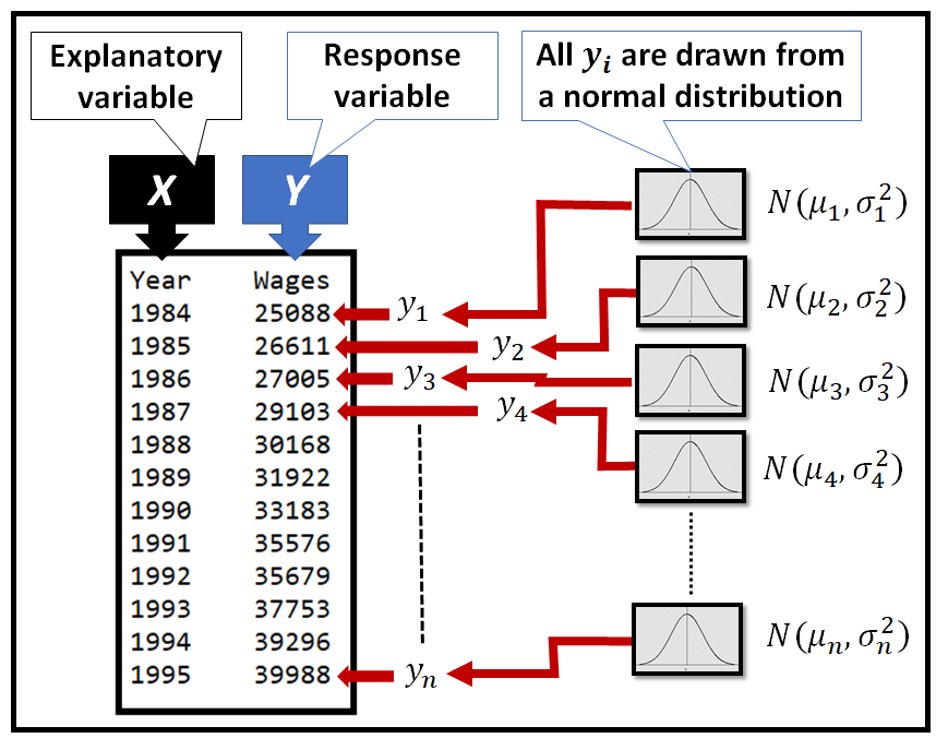
Normality in the context of linear regression
While building a linear regression model, one assumes that Y depends on a matrix of regression variables X. This makes Y conditionally normal on X. If X =[x_1, x_2, …, x_n] are jointly normal, then µ = f(X) is a normally distributed vector, and so is Y, as follows:

Why test for normality?
Several statistical techniques and models assume that the underlying data is normally distributed.
I’ll give below three such situations where normality rears its head:
- As seen above, in Ordinary Least Squares (OLS) regression, Y is conditionally normal on the regression variables X in the following manner: Y is normal, if X =[x_1, x_2, …, x_n] are jointly normal. But nothing bad happens to your OLS model, even if Y isn’t normally distributed.
- A non-strict requirement of classical linear regression models is that the residual errors of regression ‘ϵ=(yobs-ypredicted)’ should be normally distributed with an expected value of zero i.e. E(ϵ) = 0. If the residual errors ϵ are not normally distributed, one cannot reliably calculate confidence intervals for the model’s forecasts using the t-distribution, especially for small sample sizes (n ≤ 20).
Bear in mind that even if the errors are not normally distributed, the OLS estimator is still the BLUE i.e. Best Linear Unbiased Estimator for the model as long as E(ϵ)=0, and all other requirements of OLSR are satisfied.
- Finally, certain goodness-of-fit techniques such as the F-test for regression analysis assume that the residual errors of the competing regression models are all normally distributed. If the residual errors are not normally distributed, the F-test cannot be reliably used to compare the goodness-of-fit of two competing regression models.
How can I tell if my data is (not) normally distributed?
Several statistical tests are available to test the degree to which your data deviates from normality, and if the deviation is statistically significant.
We’ll look at moment based measures, namely Skewness and Kurtosis, and the statistical tests of significance, namely Omnibus K² and Jarque — Bera, that are based on these measures.
What is ‘Skewness’ and how to use it?
Skewness lets you test by how much the overall shape of a distribution deviates from the shape of the normal distribution.
The following figures illustrate skewed distributions.
The moment based definition of Skewness is as follows:
Skewness is defined as the third standardized central moment, of the random variable of the probability distribution.
The formula for skewness of the population is show below:
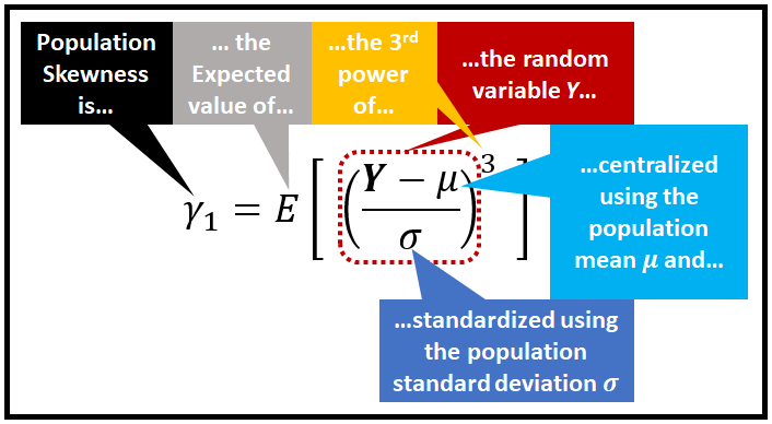
Skewness has the following properties:
- Skewness is a moment based measure (specifically, it’s the third moment), since it uses the expected value of the third power of a random variable.
- Skewness is a central moment, because the random variable’s value is centralized by subtracting it from the mean.
- Skewness is a standardized moment, as its value is standardized by dividing it by (a power of) the standard deviation.
- Because it is the third moment, a probability distribution that is perfectly symmetric around the mean will have zero skewness. This is because, for each y_i that is greater than the mean µ, there will be a corresponding y_i smaller than mean µ by the same amount. Since the distribution is symmetric around the mean, both y_i values will have the same probability. So pairs of (y_i- µ) will cancel out, yielding a total skewness of zero.
- Skewness of the normal distribution is zero.
- While a symmetric distribution will have a zero skewness, a distribution having zero skewness is not necessarily symmetric.
- Certain ratio based distributions — most famously the Cauchy distribution — have an undefined skewness as they have an undefined mean µ.
In practice, we can estimate the skewness in the population by calculating skewness for a sample. For the sample, we cheat a little by assuming that the random variable is uniformly distributed, so the probability of each y_i in the sample is 1/n and the third, central, sample moment becomes 1/n times a simple summation over all (y_i —y_bar)³.

Skewness is very sensitive to the parameters of the probability distribution.
The following figure illustrates the skewness of the Poisson distribution’s Probability Mass Function for various values of the event rate parameter λ:

Why does skewness of Poisson’s PMF reduce for large event rates? For large values of λ, the Poisson distribution’s PMF approaches the Normal distribution’s PMF with mean and variance = λ. That is, Poisson(λ) → N(λ, λ), as λ → ∞. Therefore, it’s no coincidence what are seeing in the above figure.
As λ → ∞, skewness of the Poisson distribution tends to the skewness of the normal distribution, namely 0.
There are other measures of Skewness also, for example:
- Skewness of mode
- Skewness of median
- Skewness calculated in terms of the Quartile values
- …and a few others.
What is ‘Kurtosis’ and how to use it?
Kurtosis is a measure of how differently shaped are the tails of a distribution as compared to the tails of the normal distribution. While skewness focuses on the overall shape, Kurtosis focuses on the tail shape.
Kurtosis is defined as follows:
Kurtosis is the fourth standardized central moment, of the random variable of the probability distribution.
The formula for Kurtosis is as follows:

Kurtosis has the following properties:
- Just like Skewness, Kurtosis is a moment based measure and, it is a central, standardized moment.
- Because it is the fourth moment, Kurtosis is always positive.
- Kurtosis is sensitive to departures from normality on the tails. Because of the 4th power, smaller values of centralized values (y_i-µ) in the above equation are greatly de-emphasized. In other words, values in Y that lie near the center of the distribution are de-emphasized. Conversely, larger values of (y_i-µ), i.e. the ones lying on the two tails of the distribution are greatly emphasized by the 4th power. This property makes Kurtosis largely ignorant about the values lying toward the center of the distribution, and it makes Kurtosis sensitive toward values lying on the distribution’s tails.
- Kurtosis of the normal distribution is 3.0. While measuring the departure from normality, Kurtosis is sometimes expressed as excess Kurtosis which is the balance amount of Kurtosis after subtracting 3.0.
For a sample, excess Kurtosis is estimated by dividing the fourth central sample moment by the fourth power of the sample standard deviation, and subtracting 3.0, as follows:

Here is an excellent image from Wikipedia Commons that shows the Excess Kurtosis of various distributions. I have super-imposed a magnified version of the tails in the top left side of the image:
Normality tests based on Skewness and Kurtosis
While Skewness and Kurtosis quantify the amount of departure from normality, one would want to know if the departure is statistically significant. The following two tests let us do just that:
- The Omnibus K-squared test
- The Jarque–Bera test
In both tests, we start with the following hypotheses:
- Null hypothesis (H_0): The data is normally distributed.
- Alternate hypothesis (H_1): The data is not normally distributed, in other words, the departure from normality, as measured by the test statistic, is statistically significant.
Omnibus K-squared normality test
The Omnibus test combines the random variables for Skewness and Kurtosis into a single test statistic as follows:

Probability distribution of the test statistic:
In the above formula, the functions Z1() and Z2() are meant to make the random variables g1 and g2 approximately normally distributed. Which in turn makes their sum of squares approximately Chi-squared(2) distributed, thereby making the statistic of the Omnibus K-squared approximately Chi-squared(2) distributed under the assumption that null hypothesis is true, i.e. the data is normally distributed.
Jarque–Bera normality test
The test statistic for this test is as follows:

Probability distribution of the test statistic:
The test statistic is the scaled sum of squares of random variables g1 and g2 that are each approximately normally distributed, thereby making the JB test statistic approximately Chi-squared(2) distributed, under the assumption that the null hypothesis is true.
Example
We’ll use the following data set from the U.S. Bureau of Labor Statistics, to illustrate the application of normality tests:
Here are the first few rows of the data set:
You can download the data from this link.
Let’s fit the following OLS regression model to this data set:
Wages = β_0 + β_1*Year+ ϵ
Where:
Wages is the response a.k.a. dependent variable,
Year is the regression a.k.a. explanatory variable,
β_0 is the intercept of regression,
β_1 is the coefficient of regression, and
ϵ is the unexplained regression error
We’ll use Python libraries pandas and statsmodels to read the data, and to build and train our OLS model for this data.
Let’s start with importing the required packages:
import pandas as pd
import statsmodels.formula.api as smf
import statsmodels.stats.api as sms
from statsmodels.compat import lzip
import matplotlib.pyplot as plt
from statsmodels.graphics.tsaplots import plot_acf
Read the data into the pandas data frame:
df = pd.read_csv('wages_and_salaries_1984_2019_us_bls_CXU900000LB1203M.csv', header=0)
Plot Wages against Year:
fig = plt.figure()

plt.xlabel('Year')
plt.ylabel('Wages and Salaries (USD)')

fig.suptitle('Wages and Salaries before taxes. All US workers')

wages, = plt.plot(df['Year'], df['Wages'], 'go-', label='Wages and Salaries')

plt.legend(handles=[wages])

plt.show()

Create the regression expression in Patsy syntax. In the following expression, we are telling statsmodels that Wages is the response variable and Year is the regression variable. statsmodels will automatically add an intercept to the regression equation.
Configure the OLS regression model by passing the model expression, and train the model on the data set, all in one step:
olsr_results = smf.ols(expr, df).fit()
Print the model summary:
print(olsr_results.summary())
In the following output, I have called out the areas that bode well and bode badly for our OLS model’s suitability for the data:

Interpreting the results
Following are a few things to note from the results:
- The residual errors are positively skewed with a skewness of 0.268 and they also have an excess positive Kurtosis of 2.312 i.e. thicker tails.
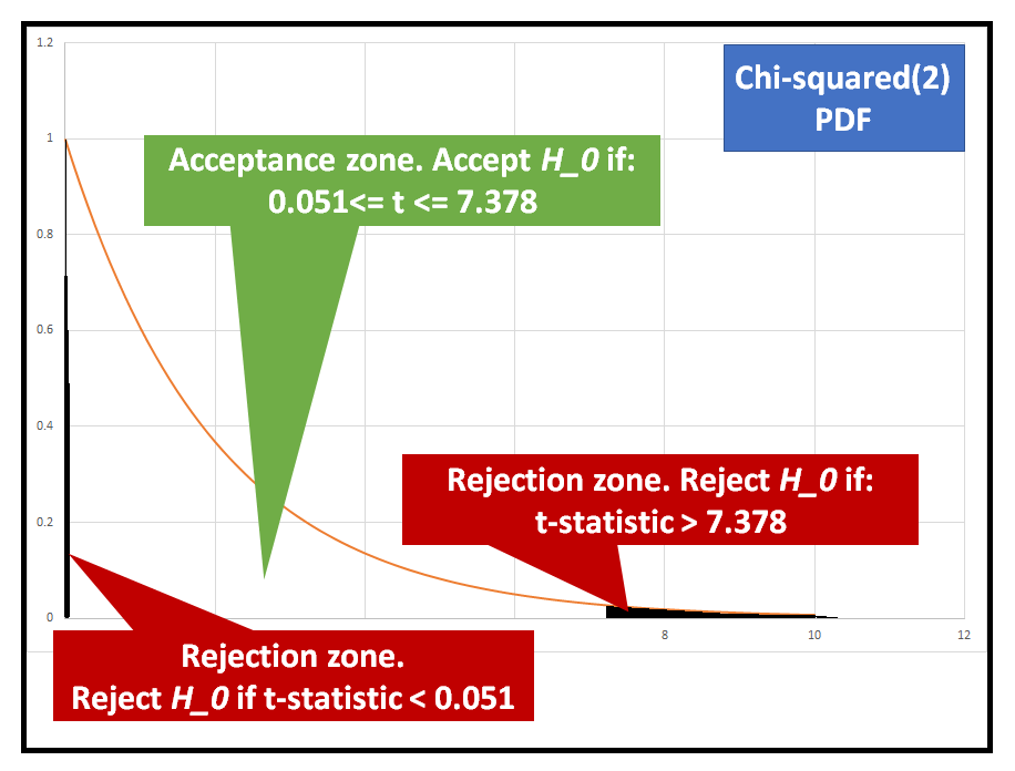
- The Omnibus test and the JB test have both produced test-statistics (1.219 and 1.109 respectively), which lie within the H_0 acceptance zone of the Chi-squared(2) PDF (see figure below). Thus we will accept the hypothesis H_0, i.e. the residuals are normally distributed.
- You can also get the values of Skewness, excess Kurtosis, and the test statistics for Omnibus and JB tests as follows:
name = ['Omnibus K-squared test', 'Chi-squared(2) p-value']

#Pass the residual errors of the regression into the test
test = sms.omni_normtest(olsr_results.resid)

lzip(name, test)
This prints out the following:
> [('Omnibus K-squared test', 1.2194658631806088), ('Chi-squared(2) p-value', 0.5434960003061313)]
name = ['Jarque-Bera test', 'Chi-squared(2) p-value', 'Skewness', 'Kurtosis']
test = sms.jarque_bera(olsr_results.resid)
lzip(name, test)
This prints out the following:
[('Jarque-Bera test', 1.109353094606092), ('Chi-squared(2) p-value', 0.5742579764509973), ('Skewness', 0.26780140709870015), ('Kurtosis', 2.3116476989966737)]
- Since the residuals seem to be normally distributed, we can also trust the 95% confidence levels reported by the model for the two model params.
- We can also trust the p-value of the F-test. It’s exceedingly tiny, indicating that the both model params are also jointly significant.
- Finally, the R-squared reported by the model is quite high indicating that the model has fitted the data well.
Now for the bad part: Both the Durbin-Watson test and the Condition number of the residuals indicates auto-correlation in the residuals, particularly at lag 1.
We can easily confirm this via the ACF plot of the residuals:
plot_acf(olsr_results.resid, title='ACF of residual errors')
plt.show()

This presents a problem for us: One of the fundamental requirements of Classical Linear Regression Models is that the residual errors should not be auto-correlated. In this case they most certainly are so. Which means that the OLS estimator may have under-estimated the variance in the training data, which in turn means that it’s predictions will be off by a large amount.
Simply put, the OLS estimator is no longer BLUE (Best Linear Unbaised Estimator) for the model. Bummer!
The auto-correlation of residual errors points to a possibility that our model was incorrectly chosen, or incorrectly configured. Particularly,
- We may have left out some key explanatory variables which is causing some signal to leak into the residuals in the form of auto-correlations, OR,
- The choice of the OLS model itself may be entirely wrong for this data set. We may need to look at alternate models such as the Regression with ARIMA Errors model which we had covered in an earlier section.
In such cases, your choice is between accepting the sub optimal-ness of the chosen model, and addressing the above two reasons for sub optimality.
Summary
- Several statistical procedures assume that the underlying data follows the normal distribution.
- Skewness and Kurtosis are two moment based measures that will help you to quickly calculate the degree of departure from normality.
- In addition to using Skewness and Kurtosis, you should use the Omnibus K-squared and Jarque-Bera tests to determine whether the amount of departure from normality is statistically significant.
- In some cases, if the data (or the residuals) are not normally distributed, your model will be sub-optimal.
References, Citations and Copyrights
Data links
Wages and salaries by Occupation: Total wage and salary earners (series id: CXU900000LB1203M). U.S. Bureau of Labor Statistics under US BLS Copyright Terms. Curated data set link for download
Images
All images are copyright Sachin Date under CC-BY-NC-SA, unless a different source and copyright are mentioned underneath the image.
I write about topics in data science, with a specific focus on time series analysis, regression and forecasting.
If you liked this content, please subscribe to receive new content in your email:
UP: Table of Contents