From Wikipedia, the free encyclopedia

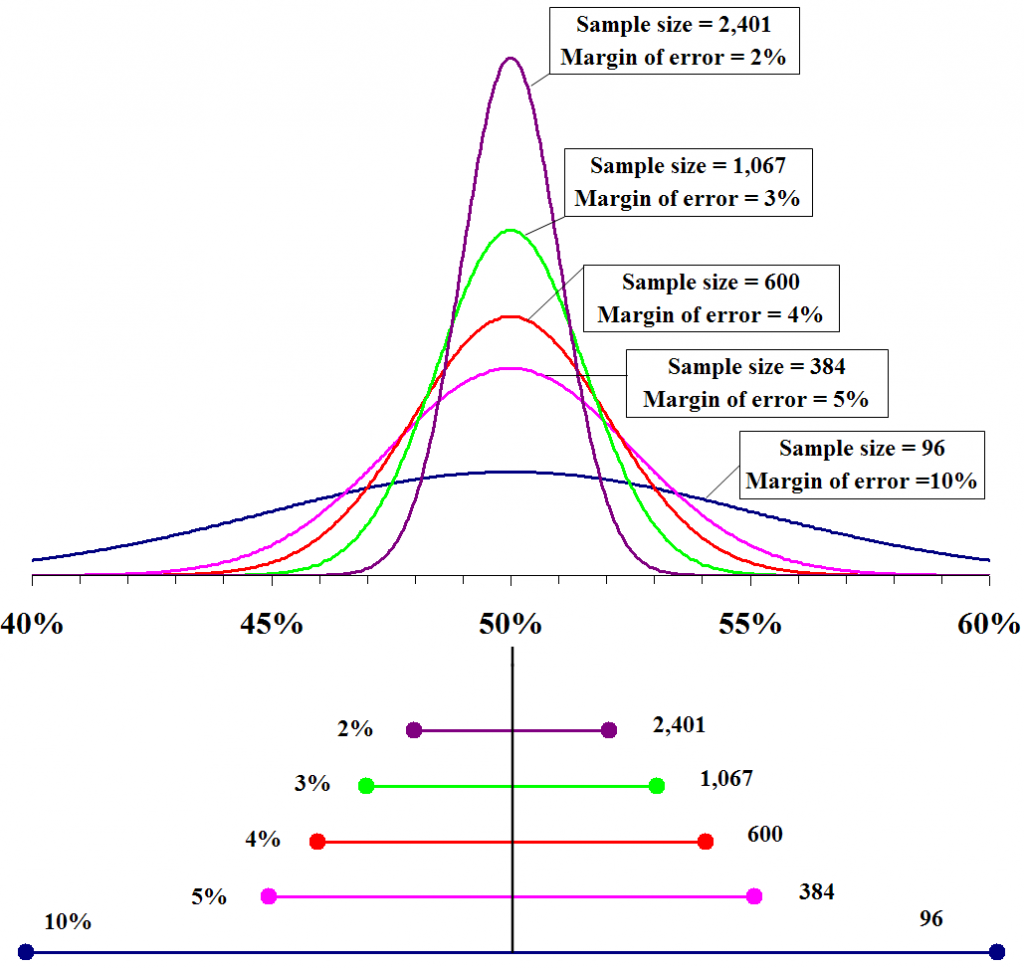
Probability densities of polls of different sizes, each color-coded to its 95% confidence interval (below), margin of error (left), and sample size (right). Each interval reflects the range within which one may have 95% confidence that the true percentage may be found, given a reported percentage of 50%. The margin of error is half the confidence interval (also, the radius of the interval). The larger the sample, the smaller the margin of error. Also, the further from 50% the reported percentage, the smaller the margin of error.
The margin of error is a statistic expressing the amount of random sampling error in the results of a survey. The larger the margin of error, the less confidence one should have that a poll result would reflect the result of a census of the entire population. The margin of error will be positive whenever a population is incompletely sampled and the outcome measure has positive variance, which is to say, the measure varies.
The term margin of error is often used in non-survey contexts to indicate observational error in reporting measured quantities.
Concept[edit]
Consider a simple yes/no poll  as a sample of
  respondents drawn from a population
  reporting the percentage
  of yes responses. We would like to know how close is to the true result of a survey of the entire population
  , without having to conduct one. If, hypothetically, we were to conduct poll over subsequent samples of respondents (newly drawn from ), we would expect those subsequent results
  to be normally distributed about
  . The margin of error describes the distance within which a specified percentage of these results is expected to vary from .
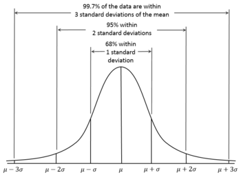
According to the 68-95-99.7 rule, we would expect that 95% of the results will fall within about two standard deviations ( ) either side of the true mean . This interval is called the confidence interval, and the radius (half the interval) is called the margin of error, corresponding to a 95% confidence level.
Generally, at a confidence level  , a sample sized of a population having expected standard deviation
  has a margin of error

where  denotes the quantile (also, commonly, a z-score), and
  is the standard error.
Standard deviation and standard error[edit]
We would expect the normally distributed values to have a standard deviation which somehow varies with . The smaller , the wider the margin. This is called the standard error  .
.
For the single result from our survey, we assume that  , and that all subsequent results together would have a variance
  .
.

Note that  corresponds to the variance of a Bernoulli distribution.
Maximum margin of error at different confidence levels[edit]
For a confidence level , there is a corresponding confidence interval about the mean  , that is, the interval
 ![{displaystyle [mu -z_{gamma }sigma ,mu +z_{gamma }sigma ]}](https://wikimedia.org/api/rest_v1/media/math/render/svg/a4568060e0cffbc8dfb793aa2ef4617c89cb9e94) within which values of should fall with probability . Precise values of are given by the quantile function of the normal distribution (which the 68-95-99.7 rule approximates).
within which values of should fall with probability . Precise values of are given by the quantile function of the normal distribution (which the 68-95-99.7 rule approximates).
Note that is undefined for  , that is,
  is undefined, as is
  .
.
|
|
|
|
|
|
|---|---|---|---|---|
| 0.68 | 0.994457883210 | 0.999 | 3.290526731492 | |
| 0.90 | 1.644853626951 | 0.9999 | 3.890591886413 | |
| 0.95 | 1.959963984540 | 0.99999 | 4.417173413469 | |
| 0.98 | 2.326347874041 | 0.999999 | 4.891638475699 | |
| 0.99 | 2.575829303549 | 0.9999999 | 5.326723886384 | |
| 0.995 | 2.807033768344 | 0.99999999 | 5.730728868236 | |
| 0.997 | 2.967737925342 | 0.999999999 | 6.109410204869 |

Since  at
at  , we can arbitrarily set
  , calculate
  , , and
  to obtain the maximum margin of error for at a given confidence level and sample size , even before having actual results. With


Also, usefully, for any reported 

Specific margins of error[edit]
If a poll has multiple percentage results (for example, a poll measuring a single multiple-choice preference), the result closest to 50% will have the highest margin of error. Typically, it is this number that is reported as the margin of error for the entire poll. Imagine poll reports  as
as 
 (as in the figure above)


As a given percentage approaches the extremes of 0% or 100%, its margin of error approaches ±0%.
Comparing percentages[edit]
Imagine multiple-choice poll reports as  . As described above, the margin of error reported for the poll would typically be
  , as
, as  is closest to 50%. The popular notion of statistical tie or statistical dead heat, however, concerns itself not with the accuracy of the individual results, but with that of the ranking of the results. Which is in first?
If, hypothetically, we were to conduct poll over subsequent samples of respondents (newly drawn from ), and report result  , we could use the standard error of difference to understand how
  is expected to fall about
  . For this, we need to apply the sum of variances to obtain a new variance,
  ,
,

where  is the covariance of
  and
and  .
.
Thus (after simplifying),


Note that this assumes that  is close to constant, that is, respondents choosing either A or B would almost never chose C (making and close to perfectly negatively correlated). With three or more choices in closer contention, choosing a correct formula for becomes more complicated.
Effect of finite population size[edit]
The formulae above for the margin of error assume that there is an infinitely large population and thus do not depend on the size of population , but only on the sample size . According to sampling theory, this assumption is reasonable when the sampling fraction is small. The margin of error for a particular sampling method is essentially the same regardless of whether the population of interest is the size of a school, city, state, or country, as long as the sampling fraction is small.
In cases where the sampling fraction is larger (in practice, greater than 5%), analysts might adjust the margin of error using a finite population correction to account for the added precision gained by sampling a much larger percentage of the population. FPC can be calculated using the formula[1]

…and so, if poll were conducted over 24% of, say, an electorate of 300,000 voters,


Intuitively, for appropriately large ,


In the former case, is so small as to require no correction. In the latter case, the poll effectively becomes a census and sampling error becomes moot.
See also[edit]
- Engineering tolerance
- Key relevance
- Measurement uncertainty
- Random error
References[edit]
- ^ Isserlis, L. (1918). «On the value of a mean as calculated from a sample». Journal of the Royal Statistical Society. Blackwell Publishing. 81 (1): 75–81. doi:10.2307/2340569. JSTOR 2340569. (Equation 1)
Sources[edit]
- Sudman, Seymour and Bradburn, Norman (1982). Asking Questions: A Practical Guide to Questionnaire Design. San Francisco: Jossey Bass. ISBN 0-87589-546-8
- Wonnacott, T.H.; R.J. Wonnacott (1990). Introductory Statistics (5th ed.). Wiley. ISBN 0-471-61518-8.
External links[edit]
- «Errors, theory of», Encyclopedia of Mathematics, EMS Press, 2001 [1994]
- Weisstein, Eric W. «Margin of Error». MathWorld.
In this article we will give you all the vital information on the “margin of error in statistics” This is very vast to compile in just one small article but still we will give you all the essential information just give complete reading to this piece of compilation.
We will be covering all these questions like what is the margin of error in statistics, How to Calculate Margin of Error, How to Calculate Margin of Error: Steps, Some Relationships, Margin of Error Calculation and some more related information/formulas.
What is a margin Error?
The range of values below and above the sample statistic in a confidence interval is called the margin of error. We can also define confidence interval as the way to show the uncertainty with a certain static. for Example from a poll result we get that 98% of confidence interval of 4.88 and 5.26. And if the poll is repeat again using the same parameter and technique. Then we will definitely get results in the interval 4.88 to 5.26 98% of the times.
What is Margin of Error Percentage ?
Margin of error is defined as the difference between true population. And the estimated population from poll result is called “Error percentage of margin”. We can calculate margin of error using these formulas given below :
Margin of error = Product of Critical value and Standard deviation or Margin of error = Product of Critical value and Standard error of the statistic.
How to calculate the margin of error: Steps
Step 1
Calculate the critical value.
Step 2
Calculate the standard deviation or the standard Error.
Step 3
Calculate the Product of critical value with standard deviation or the standard Error. For example critical value= 1.5 and Standard deviation=0.06 then the margin of error calculation will be 0.09.
calculate using t-distribution calculator on this site find the t-score and the variance and standard deviation calculator will calculator will find the standard deviation from sample.
Margin of Error for a Proportion
To calculator proportion we need sample proportion, sample size and z-score
Where Z is the Z-score.
is the Sample proportion.
n is sample space.
For Example.
A group of people did a survey on 1000 scientists and 380 of thought that climate change was not caused by human pollution. Find the MoE for a 90% confidence interval
Calculate P-hat
Calculate P-hat(sample proportion) by dividing the no. of people who agreed climate change was not caused by human pollution. It means that they answered according to the statement in this example 38% scientist responded positively.
Calculate Z-Score
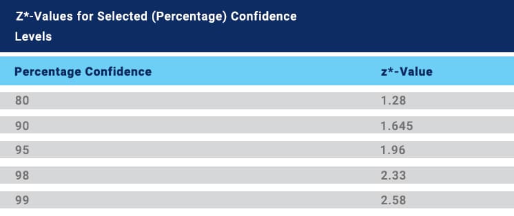
Calculate the z-score that goes with confidence interval. you’ll need to reference this critical values. A 90% confidence interval has a z-score of 1.64.
Use Margin of Error Formula
Using the formula of the margin of error find the value.
=1.64√[{0.38(0.62)}1000]
=1.64*0.0153=0.0252
Get the Result
Calculate the percentage of the step 3 and then we get thee value of the margin of error is 2.52%.
Statistics aren’t accurate Use of margin of Error
- It is a very useful method for estimating any value in this method like Calculations assuming random sampling, Different confidence levels plays an important role and also effect of sample size matters a lot. And as the heading the static are never accurate use of margin of error provide better resolution to the estimated result from any polls or survey.
- Also this process is easy to estimate as we don’t have to cover the entire size of the things rather we just have to focus on the small sample part of the entire thing and this small sample represents the entire thing. Besides, this way the cost of surveying the entire population.
Conclusion
Now you might be quite confident about the margin of error in statistics. Next time don’t get into trouble while talking about the margin of error in statistics.
Furthermore, get the best math assignment help from the most reliable math assignment helpers in the world.
More Question on Margin of Error in Statistics
What is a margin Error?
The range of values below and above the sample statistic in a confidence interval is called the margin of error.
What is Margin of Error Percentage ?
Margin of error is defined as the difference between true population. And the estimated population from poll result is called “Error percentage of margin”.
In statistics, margin of error is used to assess how precise some estimate is of a population proportion or a population mean.
We use typically use margin of error when calculating confidence intervals for population parameters.
The following examples show how to calculate and interpret margin of error for a population proportion and a population mean.
Example 1: Interpret Margin of Error for Population Proportion
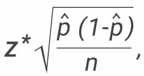
We use the following formula to calculate a confidence interval for a population proportion:
Confidence Interval = p +/- z*(√p(1-p) / n)
where:
- p: sample proportion
- z: the chosen z-value
- n: sample size
The portion of the equation that comes after the +/- sign represents the margin of error:
Margin of Error = z*(√p(1-p) / n)
For example, suppose we want to estimate the proportion of residents in a county that are in favor of a certain law. We select a random sample of 100 residents and ask them about their stance on the law.
Here are the results:
- Sample size n = 100
- Proportion in favor of law p = 0.56
Suppose we would like to calculate a 95% confidence interval for the true proportion of residents in the county that are in favor of the law.
Using the formula above, we calculate the margin of error to be:
- Margin of Error = z*(√p(1-p) / n)
- Margin of Error = 1.96*(√.56(1-.56) / 100)
- Margin of Error = .0973
We can then calculate the 95% confidence interval to be:
- Confidence Interval = p +/- z*(√p(1-p) / n)
- Confidence Interval = .56 +/- .0973
- Confidence Interval = [.4627, .6573]
The 95% confidence interval for the proportion of residents in the county who are in favor of the law turns out to be [.4627, .6573].
This means we’re 95% confident that the true proportion of residents who support the law is between 46.27% and 65.73%.
The proportion of residents in the sample who were in favor of the law was 56%, but by subtracting and adding the margin of error to this sample proportion we’re able to construct a confidence interval.
This confidence interval represents a range of values that are highly likely to contain the true proportion of residents in the county who are in favor of the law.
Example 2: Interpret Margin of Error for Population Mean
We use the following formula to calculate a confidence interval for a population mean:
Confidence Interval = x +/- z*(s/√n)
where:
- x: sample mean
- z: the z-critical value
- s: sample standard deviation
- n: sample size
The portion of the equation that comes after the +/- sign represents the margin of error:
Margin of Error = z*(s/√n)
For example, suppose we want to estimate the mean weight of a population of dolphins. We collect a random sample of dolphins with the following information:
- Sample size n = 40
- Sample mean weight x = 300
- Sample standard deviation s = 18.5
Using the formula above, we calculate the margin of error to be:
- Margin of Error = z*(s/√n)
- Margin of Error = 1.96*(18.5/√40)
- Margin of Error = 5.733
We can then calculate the 95% confidence interval to be:
- Confidence Interval = x +/- z*(s/√n)
- Confidence Interval = 300 +/- 5.733
- Confidence Interval =[294.267, 305.733]
The 95% confidence interval for the mean weight of dolphins in this population turns out to be [294.267, 305.733].
This means we’re 95% confident that the true mean weight of dolphins in this population is between 294.267 pounds and 305.733 pounds.
The mean weight of dolphins in the sample was 300 pounds, but by subtracting and adding the margin of error to this sample mean we’re able to construct a confidence interval.
This confidence interval represents a range of values that are highly likely to contain the true mean weight of dolphins in this population.
Additional Resources
The following tutorials provide additional information about margin of error:
Margin of Error vs. Standard Error: What’s the Difference?
How to Find Margin of Error in Excel
How to Find Margin of Error on a TI-84 Calculator
What is a Margin of Error?
A margin of error is a statistical measurement that accounts for the difference between actual and projected results in a random survey sample. In simpler terms, the margin of error allows you to gauge the level of unpredictability in data and research outcomes.
For example, let’s say a researcher gives the mean estimate for a survey as 50 with a margin of error of ±5. This means that the actual mean, when calculated, could be any value from 45–55.
The margin of error of a data set directly influences the confidence level of the investigator in the research outcomes. Typically, if your research outcome or survey results have a higher margin of error, it means that the data sets might be unreliable. On the other hand, a lower margin of error indicates that the results truly represent the research population.
Importance of Margin of Error in Surveys, Research, and Polls
1. Margin of Error Helps You Achieve Reliable Outcomes in Research
Margin of error accounts for any disparities between results from the research sample and the target population. Typically, the higher the margin of error, the greater the difference between actual and estimated outcomes, further suggesting that the survey results are less likely to be true for the entire population.
2. It Helps the Researcher Determine How Representative the Sample Is
A low margin of error shows that the sample population closely represents the population of interest in a systematic investigation.
When dealing with a large population of interest, it is impossible to collect data from every variable. So, the researcher has to select a sample population that represents all the subgroups in the original population of interest.
If the sample population excludes some of the groups, then the final results of the poll, survey, or research will not reflect the actual outcome of the original population.
3. Margin of Error Helps You Determine the Confidence Level and Confidence Interval of Your Data Sets
When you know the margin of error of your survey and the value of your observed score, you can easily determine your data set’s confidence interval. Confidence interval is a statistical range of the possible values of a parameter. In contrast, confidence level measures the accuracy rate of your research outcomes of survey results based on the available data.
How to Calculate the Margin of Error
To determine the margin of error of your data sets, you need to ensure that the selected research sample truly represents your population of interest. This starts from identifying the right population of interest to applying the appropriate sampling technique.
Once you have a well-representative sample, you can go ahead to calculate the margin of error using the following formula:
Where;
P-hat = Sample Proportion
n = Sample Size
z = Z-Score
Here’s an example of how to apply this formula to your data.
Let’s say you conducted a poll on how many people use Snapchat for business. Out of 1,000 respondents, 450 chose “yes.” You also have a confidence level of 90%.
Step 1: Determine P-hat
P-hat = Numbers of respondents who chose yes ÷ Total number of respondents
P-hat = 450 ÷ 1000 = 0.45 or 45%
Step 2: Find the Z-Score of the corresponding confidence level. Using this Z-Score table, the Z-score of 90 is 1.645.
Step 3: Apply the Margin of Error formula.
Margin of Error = Z-score × [√P-hat (1–P-hat)] ÷ n]
1.645 × [√(0.45 × 0.55) ÷ 1000]
Margin of Error = 2.6%
Alternatively, you can calculate the margin of error using the standard deviation of your data. This means:
Margin of Error = Z-Score × (S ÷ √n)
If you’d rather not bother with manual calculations, you can use this margin of error calculator to determine the value for your data set.
How to Interpret Margin of Error
What does it mean when your data has a margin of error to a certain percentage? More importantly, how do you interpret this in layman terms to an audience that isn’t “statistics savvy?”
The first thing you should communicate is that margin of error accounts for the maximum difference between outcomes from your sample size and that of the population of interest. So, if you have a margin of error of ±3%, it means the actual results from your target population could be 3% more or less than the estimated value.
For example, suppose your survey shows that 62% of your sample size smoke cigarettes. When you extrapolate this data to the actual population, you would have to add and subtract the margin of error, which means the actual data would fall between 59% and 65%.
Related Statistical Variables in Margin of Error
1. Arithmetic Mean
Arithmetic mean is a statistical measure of distribution that accounts for the average of all the variables in a data set. In other words, arithmetic mean allows you to find the central value of a finite set of variables.
Often, you’d need the mean of your day sets for calculating the measure of error, especially if you need to determine the standard deviation of your data first.
Arithmetic Mean Formula
Arithmetic Mean = Sum of all Variables ÷ Number of Variables
Suppose you have a date set with the following values: 13, 5, 19, 7, 12.
Arithmetic Mean = (13+5+19+7+12) ÷ 5 = 11.2
Importance of Arithmetic Mean
- It helps to reduce the margin of error of your data sets, leading to more reliable results.
- It allows you to determine the central frequency of a distribution of data.
2. Confidence Intervals vs. Confidence Levels
Confidence interval and confidence level are often used interchangeably, but they do not mean the same thing. Let’s look at some key differences.
Definition
A confidence interval is a range of results from a poll, experiment, or survey that the researcher expects to contain the population parameter of interest. Typically, researchers use the confidence interval of observation to determine whether a parameter will fall between a pair of values around the mean.
On the other hand, the confidence level is the degree of certainty or probability that a survey will produce the same results repeatedly. Theoretically, a confidence level is a measure of accuracy for research outcomes and survey results.
Measurement
Confidence levels are measured in percentages, while confidence intervals are measured in ranges. This means that the confidence level of a data set can be 90% while the confidence interval is 45±50.
Formula
Confidence Interval (C.I) = X ± Z × (S÷√n)
Where;
X = Arithmetic Mean
Z = Confidence Level Value
S = Sample Standard Deviation
n = Sample Size
Since you cannot calculate the confidence level of any observation, most researchers choose an estimated value based on the type of research, sampling technique, and the like. Many times, this ends up as 95%.
Advantages of Confidence of Interval
Confidence interval attaches a measure of accuracy to your sample data. It also helps you to evaluate the reliability of the different variables in an observation.
Advantages of Confidence Level
Like confidence intervals, confidence level allows you to measure the level of accuracy of your data. In addition, it helps you to know if the sample mean is a good or poor representation of the population mean.
3. Standard Deviation
The standard deviation of observation is the amount of variation or dispersion of values around its mean. In other words, it tells you how far apart each value or variable lies from the mean of the same data set. Typically, the higher the standard deviation, the more dispersed the data is.
Understanding standard deviation is an essential part of calculating the margin of error for your data. If you do not have the value for your sample data proportion, you can use standard deviation to determine the margin of error.
Standard Deviation Formula
Where;
s = sample standard deviation
∑ = sum of…
X = each value
x̅ = sample mean
n = number of values in the sample
Importance of Standard of Deviation
- It gives you a clear idea of the distribution of data in your observation.
- Standard Deviation measures the spread of individual data points.
4. Population Size vs. Sample Size
Also referred to as population of interest, population size is the entire group with the measurable quality or parameter your research is based on. For example, if you’re researching birds of prey in Africa, your population size would be all kinds of birds of prey on the continent.
The sample size is the subset of your population of interest who become direct participants in the research. For example, out of all the birds of prey, you could narrow your research to the African Hawk Eagle in Angola.
5. Critical Value
A critical value is the split point in hypothesis testing that determines whether the researcher accepts or rejects the null hypothesis. When plotted on a graph, the critical value separates the variables into several sections, including the rejection regions. When calculating the margin of error, researchers use the critical value to determine the applicable ranges within the data sets.
Importance of Critical Value
- It maps out the range of a confidence interval of observation.
- Critical value plays a vital role in significant testing.
6. Z-score
Z-score or standard score accounts for the difference between a given data point and the mean in an observation. It accounts for the standardization of the different data points in the distribution, allowing you to compare scores on other variables.
Importance of Z-Score
- It allows you to compare variables from different distributions.
- Z-score allows the researcher to calculate the probability of a score occurring within a typical data set.
Margin of Error vs. Standard Error
Because of their similarities, it’s pretty easy for students and researchers to mistake the margin of error for standard error and vice versa. In this section, we’ll look at some key differences between standard error and margin of error. Let’s start with their definitions.
Definition
A margin of error is a statistical measure that accounts for the degree of error received from the outcome of your research sample. On the other hand, standard error measures the accuracy of the representation of the population sample to the mean using the standard deviation of the data set.
Purpose
The purpose of the standard error is to measure the spread of random variables within your data set, while the goal of the margin of error is to estimate how much allowable difference can exist between the research population and sample size.
Formula
Margin of Error = Z-score × [√P-hat (1–P-hat)] ÷ n]
OR
Margin of Error = Z-Score × (S ÷ √n)
Where;
P-hat = Sample Proportion
n = Sample Size
z = Z-Score
S = Standard Deviation
Standard Error = Sample Standard Deviation ÷ √number of samples
Factors That Affect Margin of Error
From all we’ve discussed so far, you should already have a fair idea of the factors that primarily affect the margin of error. These factors are confidence level, sample size, and standard deviation.
It follows that increasing or decreasing any of them will have a dominant effect on the value of margin of error for your data. For example, if your sample size goes from 1,000 to 10,000, your margin of error might increase or reduce to a similar magnitude.
How to Reduce Margin of Error
Since a lower margin means a higher level of accuracy in your research results and sample, it follows that many researchers strive to reduce the margin of error in their systematic investigation. But how do you do this? Here are some ideas you can test out.
- Choose a larger sample that allows you to make more observations within your data set. This way, you can have a more exact estimate for the population parameter you’re measuring.
- Lower your confidence interval to have a more precise margin of error.
- Adopt a one-sided confidence interval which has a smaller margin of error than a two-sided confidence interval.
- Reduce the variability within your data sets, so you have more homogeneous values.
Real-Life Applications of Margin of Error
Whether in polling, market research, or simple data collection, a margin of error works in the same way—helping you determine the accuracy of your sample in relation to the actual population of interest. Let’s consider specific applications.
- Polling
In polling, a margin of error allows you to accurately extrapolate results for one option to a broader population, with minimal inaccuracy. Here’s what we mean.
Let’s say you conduct a popularity poll for two candidates. Based on the data, you peg the margin of error for Candidate A at 3%. It means there’s a close approximation between the results and the actual popularity of the candidate in the population of interest. So, you can accurately predict future variables using present polling results.
- Market Research
In market research, the margin of error shows the level of confidence an organization should have in the data collected from surveys. As mentioned earlier, the higher the margin of error, the less confident you should be in the research samples and, ultimately, the results obtained.
Conclusion
In this article, we’ve discussed the margin of error and its influence on the outcomes of any systematic investigation. Since research is based on collecting samples from a population of interest, you must account for variations between your sample data and the target audience. Calculating the margin of error of your observation is the most effective way to achieve this.
Introduction
While you are learning statistics, you will often have to focus on a sample rather than the entire population. This is because it is extremely costly, difficult and time-consuming to study the entire population. The best you can do is to take a random sample from the population – a sample that is a ‘true’ representative of it. You then carry out some analysis using the sample and make inferences about the population.
Since the inferences are made about the population by studying the sample taken, the results cannot be entirely accurate. The degree of accuracy depends on the sample taken – how the sample was selected, what the sample size is, and other concerns. Common sense would say that if you increase the sample size, the chances of error will be less because you are taking a greater proportion of the population. A larger sample is likely to be a closer representative of the population than a smaller one.
Let’s consider an example. Suppose you want to study the scores obtained in an examination by students in your college. It may be time-consuming for you to study the entire population, i.e. all students in your college. Hence, you take out a sample of, say, 100 students and find out the average scores of those 100 students. This is the sample mean. Now, when you use this sample mean to infer about the population mean, you won’t be able to get the exact population means. There will be some “margin of error”.
You will now learn the answers to some important questions: What is margin of error, what are the method of calculating margins of error, how do you find the critical value, and how to decide on t-score vs z-scores. Thereafter, you’ll be given some margin of error practice problems to make the concepts clearer.
What is Margin of Error?
The margin of error can best be described as the range of values on both sides (above and below) the sample statistic. For example, if the sample average scores of students are 80 and you make a statement that the average scores of students are 80 ± 5, then here 5 is the margin of error.
Calculating Margins of Error
For calculating margins of error, you need to know the critical value and sample standard error. This is because it’s calculated using those two pieces of information.
The formula goes like this:
margin of error = critical value * sample standard error.
How do you find the critical value, and how to calculate the sample standard error? Below, we’ll discuss how to get these two important values.
How do You find the Critical Value?
For finding critical value, you need to know the distribution and the confidence level. For example, suppose you are looking at the sampling distribution of the means. Here are some guidelines.
- If the population standard deviation is known, use z distribution.
- If the population standard deviation is not known, use t distribution where degrees of freedom = n-1 (n is the sample size). Note that for other sampling distributions, degrees of freedom can be different and should be calculated differently using appropriate formula.
- If the sample size is large, then use z distribution (following the logic of Central Limit Theorem).
It is important to know the distribution to decide what to use – t-scores vs z-scores.
Caution – when your sample size is large and it is not given that the distribution is normal, then by Central Limit Theorem, you can say that the distribution is normal and use z-score. However, when the sample size is small and it is not given that the distribution is normal, then you cannot conclude anything about the normality of the distribution and neither z-score nor t-score can be used.
When finding the critical value, confidence level will be given to you. If you are creating a 90% confidence interval, then confidence level is 90%, for 95% confidence interval, the confidence level is 95%, and so on.
Here are the steps for finding critical value:
Step 1: First, find alpha (the level of significance). alpha =1 – Confidence level.
For 95% confidence level, alpha =0.05
For 99% confidence level, alpha =0.01
Step 2: Find the critical probability p*. Critical probability will depend on whether we are creating a one-sided confidence interval or a two-sided confidence interval.
For two-sided confidence interval, p*=1-dfrac { alpha }{ 2 }
For one-sided confidence interval, p*=1-alpha
Then you need to decide on using t-scores vs z-scores. Find a z-score having a cumulative probability of p*. For a t-statistic, find a t-score having a cumulative probability of p* and the calculated degrees of freedom. This will be the critical value. To find these critical values, you should use a calculator or respective statistical tables.
Sample Standard Error
Sample standard error can be calculated using population standard deviation or sample standard deviation (if population standard deviation is not known). For sampling distribution of means:
Let sample standard deviation be denoted by s, population standard deviation is denoted by sigma and sample size be denoted by n.
text {Sample standard error}=dfrac { sigma }{ sqrt { n } }, if sigma is known
text {Sample standard error}=dfrac { s }{ sqrt { n } }, if sigma is not known
Depending on the sampling distributions, the sample standard error can be different.
Having looked at everything that is required to create the margin of error, you can now directly calculate a margin of error using the formula we showed you earlier:
Margin of error = critical value * sample standard error.
Some Relationships
1. Confidence level and marginal of error
As the confidence level increases, the critical value increases and hence the margin of error increases. This is intuitive; the price paid for higher confidence level is that the margin of errors increases. If this was not so, and if higher confidence level meant lower margin of errors, nobody would choose a lower confidence level. There are always trade-offs!
2. Sample standard deviation and margin of error
Sample standard deviation talks about the variability in the sample. The more variability in the sample, the higher the chances of error, the greater the sample standard error and margin of error.
3. Sample size and margin of error
This was discussed in the Introduction section. It is intuitive that a greater sample size will be a closer representative of the population than a smaller sample size. Hence, the larger the sample size, the smaller the sample standard error and therefore the smaller the margin of error.
Margin of Error Practice Problems
Example 1
25 students in their final year were selected at random from a high school for a survey. Among the survey participants, it was found that the average GPA (Grade Point Average) was 2.9 and the standard deviation of GPA was 0.5. What is the margin of error, assuming 95% confidence level? Give correct interpretation.
Step 1: Identify the sample statistic.
Since you need to find the confidence interval for the population mean, the sample statistic is the sample mean which is the average GPA = 2.9.
Step 2: Identify the distribution – t, z, etc. – and find the critical value based on whether you need a one-sided confidence interval or a two-sided confidence interval.
Since population standard deviation is not known and the sample size is small, use a t distribution.
text {Degrees of freedom}=n-1=25-1=24.
alpha=1-text {Confidence level}=1-0.95=0.05
Let the critical probability be p*.
For two-sided confidence interval,
p*=1-dfrac { alpha }{ 2 } =1-dfrac { 0.05 }{ 2 } =0.975.
The critical t value for cumulative probability of 0.975 and 24 degrees of freedom is 2.064.
Step 3: Find the sample standard error.
text{Sample standard error}=dfrac { s }{ sqrt { n } } =dfrac { 0.5 }{ sqrt { 25 } } =0.1
Step 4: Find margin of error using the formula:
Margin of error = critical value * sample standard error
= 2.064 * 0.1 = 0.2064
Interpretation: For a 95% confidence level, the average GPA is going to be 0.2064 points above and below the sample average GPA of 2.9.
Example 2
400 students in Princeton University are randomly selected for a survey which is aimed at finding out the average time students spend in the library in a day. Among the survey participants, it was found that the average time spent in the university library was 45 minutes and the standard deviation was 10 minutes. Assuming 99% confidence level, find the margin of error and give the correct interpretation of it.
Step 1: Identify the sample statistic.
Since you need to find the confidence interval for the population mean, the sample statistic is the sample mean which is the mean time spent in the university library = 45 minutes.
Step 2: Identify the distribution – t, z, etc. and find the critical value based on whether the need is a one-sided confidence interval or a two-sided confidence interval.
The population standard deviation is not known, but the sample size is large. Therefore, use a z (standard normal) distribution.
alpha=1-text{Confidence level}=1-0.99=0.01
Let the critical probability be p*.
For two-sided confidence interval,
p*=1-dfrac { alpha }{ 2 } =1-dfrac { 0.01 }{ 2 } =0.995.
The critical z value for cumulative probability of 0.995 (as found from the z tables) is 2.576.
Step 3: Find the sample standard error.
text{Sample standard error}=dfrac { s }{ sqrt { n } } =dfrac { 10 }{ sqrt { 400 } } =0.5
Step 4: Find margin of error using the formula:
Margin of error = critical value * sample standard error
= 2.576 * 0.5 = 1.288
Interpretation: For a 99% confidence level, the mean time spent in the library is going to be 1.288 minutes above and below the sample mean time spent in the library of 45 minutes.
Example 3
Consider a similar set up in Example 1 with slight changes. You randomly select X students in their final year from a high school for a survey. Among the survey participants, it was found that the average GPA (Grade Point Average) was 3.1 and the standard deviation of GPA was 0.7. What should be the value of X (in other words, how many students you should select for the survey) if you want the margin of error to be at most 0.1? Assume 95% confidence level and normal distribution.
Step 1: Find the critical value.
alpha=1-text{Confidence level}=1-0.95=0.05
Let the critical probability be p*.
For two-sided confidence interval,
p*=1-dfrac { alpha }{ 2 } =1-dfrac { 0.05 }{ 2 } =0.975.
The critical z value for cumulative probability of 0.975 is 1.96.
Step 3: Find the sample standard error in terms of X.
text{Sample standard error}=dfrac { s }{ sqrt { X } }=dfrac { 0.7 }{ sqrt { X } }
Step 4: Find X using margin of error formula:
Margin of error = critical value * sample standard error
0.1=1.96*dfrac { 0.7 }{ sqrt { X } }
This gives X=188.24.
Thus, a sample of 189 students should be taken so that the margin of error is at most 0.1.
Conclusion
The margin of error is an extremely important concept in statistics. This is because it is difficult to study the entire population and the sampling is not free from sampling errors. The margin of error is used to create confidence intervals, and most of the time the results are reported in the form of a confidence interval for a population parameter rather than just a single value. In this article, you made a beginning by learning answering questions like what is margin of error, what is the method of calculating margins of errors, and how to interpret these calculations. You also learned to decide whether to use t-scores vs z-scores and gained information about finding critical values. Now you know how to use margin of error for constructing confidence intervals, which are widely used in statistics and econometrics.
Let’s put everything into practice. Try this Statistics practice question:

Looking for more Statistics practice?
You can find thousands of practice questions on Albert.io. Albert.io lets you customize your learning experience to target practice where you need the most help. We’ll give you challenging practice questions to help you achieve mastery in Statistics.
Start practicing here.
Are you a teacher or administrator interested in boosting Statistics student outcomes?
Learn more about our school licenses here.
Margin of error is a statistic that states the number of errors in random sampling in a survey. Margin of error can also be defined as a distance in a certain confidence interval (statistical) from the survey, this distance represents a statistic. Margin of error measures how close the results of the sample are to the results in reality.
In statistic, we calculate the confidence interval to see where the value of the data of sample statistic will fall. The range of values which are below and above the sample statistic in a confidence interval is known as Margin of Error. In other words, it is basically the degree of error in the sample statistic.
Higher the margin of error, lesser will the confidence in the results because the degree of deviation in these results is very high. As its name suggests, the margin of error is a range of values above and below the actual results. For example, if we get a response in a survey wherein 70% people have responded “good” and margin of error is 5%, this means that in general, 65% to 75% of the population think that the answer is “good”.
Calculating Margin of Error
In calculating the error margin, the factors that influence are:
- Sample size
- The importance of problems in the sample
- Statistics or estimators themselves

The larger the sample will increasingly represent the population. But we know in taking samples and the sample itself is always biased. For that we use margin error to reduce the bias that occurs. Bias that can be known from the margin error is the bias arising from the sampling error.
Standard error of proportion and confidence interval.
To find out the margin error calculation, it must first be known about the standard error of proportion and confidence interval.
Confidence interval (CI) is a percentage that describes how close the original value is to the statistics (estimator) measured +/- margin error.
Standard error of proportions measures the accuracy of the estimator of proportions and estimates the standard deviation of percentages.
It can be predicted from p and the size of sample n, if n is small enough then use the formula:
Standard error = √p(1-p)/n
To estimate the proportions of plus and minus, the margin error is the confidence interval for the proportion or percentage. In other words, the error margin is part of the confidence interval. The error margin is calculated by multiplying the standard error with the confidence factor of a certain level of confidence. Example:
- The margin (plus – minus estimator) of 1 standard error is 68% confidence interval,
- The margin (plus – minus estimator) of 1.96 standard error is 95% confidence interval
- The margin (plus – minus estimator) of 2.58 standard error is 99% confidence interval
Maximum margin error
The maximum margin of error for proportions is the distance from the confidence interval when p = 50%. For 95% confidence, the formula is
(maximum) error margin (95%) = 1.96 x √0.5 (1-0.5) / n = 0.98 / √n
Different confidence intervals
The margin error depends on the probability of a confidence interval, like this:
- Error margin (99%) confidence = 1.29 / √n
- Error margin (95%) confidence = 0.98 / √n
- Error margin (90%) confidence = 0.82 / √n
Some mistakes people make in understanding the use of margin errors:
- Do not use or do not involve confidence intervals. You will not know what your error margin is if the confidence interval is unknown
- Many people believe that the error margin represents the entirety of the error. Even though this is not true, what is included in the margin error is the sampling error and the non sampling error cannot be seen from the margin error.
- People sometimes believe that the margin error indicates the quality of the survey, meaning that the smaller the margin error the better the quality of the survey, even though this is not true. Many factors affect the quality of the survey, such as the method used, sampling, etc.
If you like the article we can follow it through the Random Creative Blog Feed or subscribe to get information from us.

The margin of error is an essential concept for understanding the accuracy and reliability of survey data. In this article, we’ll take a closer look at its definition and its calculation while providing examples of how it’s used in research. We’ll also discuss the importance of considering the margin of error when interpreting survey results and how it can affect the conclusions drawn from the data. So, whether you’re experienced or just starting your journey, this article is a must-read for anyone looking to master the art of margin of error and ensure the accuracy and reliability of their research. Let’s get started!
What is a Margin of Error?
Definition:
The margin of error in statistics is the degree of error in results received from random sampling surveys. A higher margin of error in statistics indicates less likelihood of relying on the results of a survey or poll, i.e. the confidence on the results will be lower to represent a population. It is a very vital tool in market research as it depicts the confidence level the researchers should have in the data obtained from surveys.
A confidence interval is the level of unpredictability with a specific statistic. Usually, it is used in association with the margin of errors to reveal the confidence a statistician has in judging whether the results of an online survey or online poll are worthy to represent the entire population.
A lower margin of error indicates higher confidence levels in the produced results.
When we select a representative sample to estimate full population, it will have some element of uncertainty. We need to infer the real statistic from the sample statistic. This means our estimate will be close to the actual figure. Considering margin of error further improves this estimate.
A well-defined population is a prerequisite for calculating the margin of error. In statistics, a “population” comprises of all the elements of a particular group that a researcher intends to study and collect data. This error can be significantly high if the population is not defined or in cases where the sample selection process is not carried out properly.
Every time a researcher conducts a statistical survey, a margin of error calculation is required. The universal formula for a sample is the following:
where:
p̂ = sample proportion (“P-hat”).
n = sample size
z = z-score corresponds to your desired confidence levels.
Are you feeling a bit confused? Don’t worry! you can use our margin of error calculator.
Example for margin of error calculation
For example, wine-tasting sessions conducted in vineyards depend on the quality and taste of the wines presented during the session. These wines represent the entire production and depending on how well the visitors receive them, the feedback from them is generalized to the entire production.
The wine tasting will be effective only when visitors do not have a pattern, i.e. they’re chosen randomly. Wine goes through a process to be palatable and similarly, the visitors also must go through a process to provide effective results.
The measurement components prove whether the wine bottles are worthy to represent the entire winery’s production or not. If a statistician states that the conducted survey will have a margin of error of plus or minus 5% at a 93% confidence interval. This means that if a survey was conducted 100 times with vineyard visitors, feedback received will be within a percentage division either higher or lower than the percentage that’s accounted 93 out of 100 times.
In this case, if 60 visitors report that the wines were extremely good. As the margin of error is plus or minus 5% in a confidence interval is 93%, in 100 visitors, it’s safe to conclude that the visitors who comment that the wines were “extremely good” will be 55 or 65 (93%) of the time.
To explain this further, let’s take an example of a survey on volunteering was sent to 1000 respondents out of which 500 agreed to the statement in the survey saying that volunteering makes life better. Calculate margin of error for 95% confidence level.
Step 1: Calculate P-hat by dividing the number of respondents who agreed with the statement in the survey to the total number of respondents. In this case, = 500/1000 = 50%
Step 2: Find z-score corresponding to 95% confidence level. In this case, z score is 1.96
Step 3: Calculate by putting these values in the formula
Step 4: Convert to a percentage
Margin of error in sample sizes:
In probability sampling, each member of a population has a probability of being selected to be a part of the sample. In this method, researchers and statisticians can select members from their area of research so that the margin of error in data received from these samples is as minimum as possible.
In non-probability sampling, samples are formed based on cost-effectiveness or convenience and not on the basis of application and because of this selection process, some sections of the population may get excluded. Surveys will be effective only on filtering members according to interests and application to the survey being conducted.
The industrial standard for confidence level is 95% and these are the margin of error percentages for certain survey sample sizes:
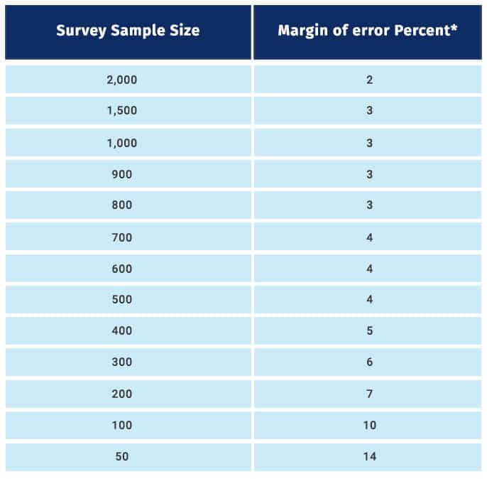
As indicated in this table, to reduce the margin of error to half, for instance, from 4 to 2, the sample size has been increased considerably, from 500 to 2000. As you must have observed, the sample size is inversely proportional to it. Till sample sizes of 1500, there is a significant decrease in it, but beyond that, this decrease reduces.
Ready to take your research game to the next level? Join QuestionPro and elevate your surveys from ho-hum to oh-wow! With our user-friendly platform, you’ll be able to create professional-grade surveys in no time. Plus, with features like customizable templates, advanced analytics, and real-time data collection, you’ll have everything you need to gather accurate, reliable data. So, don’t miss out on the fun. Join QuestionPro today for free and start discovering what your customers, employees, and communities really think. No credit card is needed.
Video transcript
— [Instructor] It is election season, and there is a runoff between candidate A versus candidate B. And we are pollsters. And we’re interested
in figuring out, well, what’s the likelihood that
candidate A wins this election? Well, ideally, we would go
to the entire population of likely voters right over here, let’s say there’s 100,000 likely voters, and we would ask every one of
the them, who do you support? And from that, we would be able to get
the population proportion, which would be, this
is the proportion that support, support candidate A. But it might not be realistic. In fact, it definitely
will not be realistic to ask, well, all 100,000 people. So instead, we do the thing that we tend to do in statistics is, is that we sample this population, and we calculate a
statistic from that sample in order to estimate this parameter. So let’s say we take a
sample right over here. So this sample size, let’s say n equals 100. And we calculate the sample proportion that support candidate A. So out of the 100, let’s say that 54 say that they’re going
to support candidate A. So the sample proportion here is 0.54. And just to appreciate that we’re not always going to get 0.54, there could’ve been a situation where we sampled a different 100, and we would’ve maybe gotten
a different sample proportion. Maybe in that one, we got 0.58. And we already have
the tools in statistics to think about this, the distribution of the possible sample proportions we could get. We’ve talked about it when we thought about
sampling distributions. So you could have the
sampling distribution of the sample proportions, of the sample proportions, proportions. And it’s going, this
distribution’s going to be specific to what our sample size is, for n is equal to 100. And so we can describe the possible sample
proportions we could get and their likelihoods with
this sampling distribution. So let me do that. So it would look something like this. Because our sample size is so much smaller than the population, it’s way less than 10%, we can assume that each
person we’re asking, that it’s approximately independent. Also, if we make the assumption
that the true proportion isn’t too close to zero
or not too close to one, then we can say that, well, look, this sampling distribution is
roughly going to be normal. So we’ll have a normal, this
kind of bell curve shape. And we know a lot about
the sampling distribution of the sample proportions. We know already, for example, and if this is foreign to
you, I encourage you to watch the videos on this on Khan Academy, that the mean of this
sampling distribution is going to be the actual
population proportion. And we also know what
the standard deviation of this is going to be. So, let me, maybe that’s
one standard deviation. This is two standard deviations. That’s three standard
deviations above the mean. That’s one standard deviation,
two standard deviations, three standard deviations below the mean. So this distance, let me do
this in a different color, this standard deviation right over here, which we denote as the
standard deviation of the sample proportions, for
this sampling distribution, this is, we’ve already
seen the formula there. It’s the square root of p times one minus p, where p is, once again,
our population proportion divided by our sample size. That’s why it’s specific
for n equals 100 here. And so in this first scenario, let’s just focus on this
one right over here, when we took a sample size of n equals 100 and we got the sample proportion of 0.54, we could’ve gotten all
sorts of outcomes here. Maybe 0.54 is right over here. Maybe 0.54 is right over here. And the reason why I
had this uncertainty is we actually don’t know what the real population parameter is, what the real population proportion is. But let me ask you maybe a
slightly easier question. What is, what is the probability, probability that our sample proportion of 0.54 is within, is within two times
two standard deviations of p? Pause the video, and think about that. Well, that’s just saying, look,
if I’m gonna take a sample and calculate the sample
proportion right over here, what’s the probability that I’m within two standard deviations of the mean? Well, that’s essentially going to be this area right over here. And we know, from studying normal curves, that approximately 95% of the area is within two standard deviations. So this is approximately 95%. 95% of the time that I
take a sample size of 100 and I calculate this sample proportion, 95% of the time, I’m going to be within
two standard deviations. But if you take this statement, you can actually construct
another statement that starts to feel a little bit more, I guess we could say inferential. We could say there, there is a 95% probability that the population proportion p is within, within two standard deviations, two standard deviations of p-hat, which is equal to 0.54. Pause this video. Appreciate that these two
are equivalent statements. If there’s a 95% chance
that our sample proportion is within two standard deviations
of the true proportion, well, that’s equivalent to
saying that there’s a 95% chance that our true proportion is
within two standard deviations of our sample proportion. And this is really, really interesting because if we were able to
figure out what this value is, well, then we would be able to create what you could call a confidence interval. Now, you immediately might
be seeing a problem here. In order to calculate this, our standard deviation
of this distribution, we have to know our population parameter. So pause this video, and think about what we would do instead. If we don’t know what p is here, if we don’t know our
population proportion, do we have something that
we could use as an estimate for our population proportion? Well, yes, we calculated p-hat already. We calculated our sample proportion. And so a new statistic
that we could define is the standard error, the standard error of
our sample proportions. And we can define that as being equal to, since we don’t know the
population proportion, we’re going to use the sample proportion, p-hat times one minus p-hat, all of that over n. In this case, of course, n is 100. We do know that. And it actually turns out, I’m not going to prove it in this video, that this actually is
an unbiased estimator for this right over here. So this is going to be equal to 0.54 times one minus 0.54, so it’s 0.46, all of that over 100. So we have the square root of .54 times .46 divided by 100, close my parentheses, Enter. So if I round to the nearest
hundredth, it’s going to be, actually, even if I round
to the nearest thousandth, it’s going to be approximately 5/100. So this is going to be, this is approximately 0.05. So another way to say all
of these things is, instead, we don’t know exactly this, but now we have an estimate for it. So we could now say with 95% confidence, and that will often be known as our confidence level right over here, with 95% confidence between, between, and so we’d want to go two standard errors below our sample proportion that we just happened to calculate. So that would be 0.54
minus two times 5/100. So that would be 0.54 minus 10/100, which would be 0.44. And we’d also want to
go two standard errors above the sample proportion. So that would be that plus 10/100. And 0.64 of voters, of voters support, support A. And so this interval that
we have right over here, from 0.44 to 0.64, this will be known as
our confidence interval, confidence interval. And this will change, not just in the starting
point and the end point, but it will change the actual length of our confidence interval, will change depending on what sample proportion we happened to pick for that sample of 100. A related idea to the confidence interval is this notion of margin of error, margin of error. And for this particular case, for this particular sample, our margin of error, because we care about 95% confidence, so that would be two standard errors. So our margin of error here is
two times our standard error, would just be 0.1 or 0.10. And so we’re going one margin of error above our sample
proportion right over here and one margin of error below our sample
proportion right over here to define our confidence interval. And as I mentioned, this
margin of error is not going to be fixed every time we take a sample. Depending on what our
sample proportion is, it’s going to affect our margin of error because that is calculated, essentially, with the standard error. Another interpretation of this is that the method that we used to get this interval right over here, the method that we used
to get this confidence, to get this confidence interval, when we use it over and over, it will produce intervals, and the intervals won’t
always be the same. It’s gonna be dependent
on our sample proportion, but it will produce intervals which include the true proportion, which we might not know
and often don’t know. It’ll include the true
proportion 95% of the time. I’ll cover that intuition
more in future videos. We’ll see how the interval changes, how the margin of error changes. But when you do this calculation over and over and over again, 95% of the time, your true proportion is
going to be contained in whatever interval you
happen to calculate that time. Now, another interesting question is, is, well, what if you wanted to tighten up the intervals on average? How would you do that? Well, if you wanted to
lower your margin of error, the best way to lower the margin of error is if you increase this
denominator right over here. And increasing that denominator means increasing the sample size. And so one thing that you will often see when people are talking
about election coverage is, well, we need to sample more people in order to get a lower margin of error. But I’ll leave you there, and I’ll see you in future videos.