Matlab как изменить цвет графика - Исправление ошибок и поиск оптимальных решений проблем

MATLAB^® creates plots using a default set of colors. The default colors provide a
clean and consistent look across the different plots you create. You can customize the
colors if you need to. Many plotting functions have an input argument such as
c or colorspec for customizing the color. The
objects returned by these functions typically have properties for controlling the color.
The names of the arguments and properties can vary, but the values they accept typically
follow a common pattern. Once you are familiar with the pattern, you can use it to
modify a wide variety of plots.

The following examples use the bar and
scatter functions to demonstrate the overall approach for
customizing colors. For a complete list of valid color values for a specific plotting
function, refer to the documentation for that function.

Types of Color Values

There are these types of color values:

Color Name or Short Name — Specify
the name of a color such as "red" or
"green". Short names specify a letter from a
color name, such as "r" or
"g".
RGB Triplet — Create a custom color
by specifying a three-element row vector whose elements are the
intensities of the red, green, and blue components of a color. The
intensities must be in the range [0,1]. For example,
you can specify a shade of pink as [1 0.5 0.8].

Some function arguments that control color do not accept RGB triplets,
but object properties that control color typically do.
Hexadecimal Color Code (Since
R2019a) — Create a custom color by
specifying a string or a character vector that starts with a hash symbol
(#) followed by three or six hexadecimal digits,
which can range from 0 to F. The
values are not case sensitive. Thus, the color codes
"#FF8800", "#ff8800",
"#F80", and "#f80" all specify
the same shade of orange.

Some function arguments that control color do not accept hexadecimal
color codes, but you can specify a hexadecimal color code using a
name-value argument that corresponds to an object property. For example,
scatter(x,y,sz,"MarkerFaceColor","#FF8800") sets
the marker color in a scatter plot to orange.

This table lists all of the valid color names and short names with the
corresponding RGB triplets and hexadecimal color codes.

Color Name	Short Name	RGB Triplet	Hexadecimal Color Code
`"red"`	`"r"`	`[1 0 0]`	`"#FF0000"`
`"green"`	`"g"`	`[0 1 0]`	`"#00FF00"`
`"blue"`	`"b"`	`[0 0 1]`	`"#0000FF"`
`"cyan"`	`"c"`	`[0 1 1]`	`"#00FFFF"`
`"magenta"`	`"m"`	`[1 0 1]`	`"#FF00FF"`
`"yellow"`	`"y"`	`[1 1 0]`	`"#FFFF00"`
`"black"`	`"k"`	`[0 0 0]`	`"#000000"`
`"white"`	`"w"`	`[1 1 1]`	`"#FFFFFF"`

Here are the RGB triplets and hexadecimal color codes for the default colors
MATLAB uses in many types of plots. These colors do not have names associated
with them.

RGB Triplet	Hexadecimal Color Code	Appearance
`[0 0.4470 0.7410]`	`"#0072BD"`
`[0.8500 0.3250 0.0980]`	`"#D95319"`
`[0.9290 0.6940 0.1250]`	`"#EDB120"`
`[0.4940 0.1840 0.5560]`	`"#7E2F8E"`
`[0.4660 0.6740 0.1880]`	`"#77AC30"`
`[0.3010 0.7450 0.9330]`	`"#4DBEEE"`
`[0.6350 0.0780 0.1840]`	`"#A2142F"`

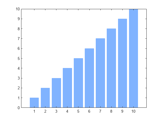
Specify Color of a Bar Chart

Create a red bar chart by calling the bar function and specifying the optional color argument as «red". Return the bar object as b, so you can customize other aspects of the chart later.

Now, change the bar fill color and outline color to light blue by setting the FaceColor and EdgeColor properties to the hexadecimal color code,»#80B3FF".

Before R2019a, specify an RGB triplet instead of a hexadecimal color code. For example, b.FaceColor = [0.5 0.7 1].

b.FaceColor = "#80B3FF";
b.EdgeColor = "#80B3FF";

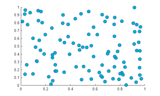
Specify Marker Colors in a Scatter Plot

Create a scatter plot of random numbers. Specify the marker size as 75 points, and use name-value arguments to specify the marker outline and fill colors. The MarkerEdgeColor property controls the outline color, and the MarkerFaceColor controls the fill color.

x = rand(1,100);
y = rand(1,100);
scatter(x,y,75,"MarkerEdgeColor","b", ...
    "MarkerFaceColor",[0 0.7 0.7])

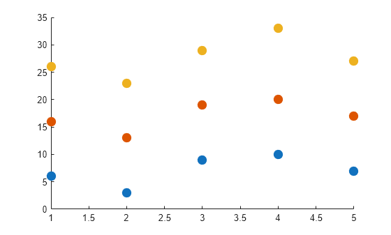
Specify Colors in a Series of Plots

There are two ways to create a series of plots:

Call a plotting function multiple times and use the hold function to retain the contents of the axes.
Pass a matrix containing multiple data series to the plotting function. The plot function has always accepted matrix inputs, and many other plotting functions also support matrix inputs.

To specify colors with either approach, call the desired plotting function with an output argument so you can access the individual plot objects. Then set properties on the plot object you want to change.

For example, create a scatter plot with 100-point filled markers. Call the scatter function with an output argument s1. Call the hold function to retain the contents of the axes, and then call the scatter function two more times with output arguments s2 and s3. The variables s1, s2, and s3 are Scatter objects.

figure
x = 1:5;
s1 = scatter(x,[6 3 9 10 7],100,"filled");
hold on
s2 = scatter(x,[16 13 19 20 17],100,"filled");
s3 = scatter(x,[26 23 29 33 27],100,"filled");
hold off

Change the color of the second Scatter object to a shade of purple.

s2.MarkerFaceColor = [0.7 0 1];

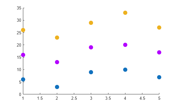
The scatter function also supports matrix inputs (since R2021a), so you can create the same plot by passing a matrix and returning a vector of objects.

figure
x = 1:5;
y = [6 3 9 10 7; 16 13 19 20 17; 26 23 29 33 27];
s = scatter(x,y,100,"filled");

To change the color of the second data series in this case, access the second Scatter object by indexing into s.

s(2).MarkerFaceColor = [0.7 0 1];

Syntax

Description

Vector and Matrix Data

example

plot(X,Y)
creates a 2-D line plot of the data in Y versus the
corresponding values in X.

To plot a set of coordinates connected by line segments, specify
X and Y as vectors of
the same length.
To plot multiple sets of coordinates on the same set of axes,
specify at least one of X or
Y as a matrix.

plot(X,Y,LineSpec)
creates the plot using the specified line style, marker, and color.

example

plot(X1,Y1,...,Xn,Yn)
plots multiple pairs of x— and
y-coordinates on the same set of axes. Use this syntax as an
alternative to specifying coordinates as matrices.

example

plot(X1,Y1,LineSpec1,...,Xn,Yn,LineSpecn)
assigns specific line styles, markers, and colors to each
x—y pair. You can specify
LineSpec for some
x—y pairs and omit it for others. For
example, plot(X1,Y1,"o",X2,Y2) specifies markers for the
first x—y pair but not for the second
pair.

example

plot(Y) plots Y
against an implicit set of x-coordinates.

If Y is a vector, the
x-coordinates range from 1 to
length(Y).
If Y is a matrix, the plot contains one line
for each column in Y. The
x-coordinates range from 1 to the number of rows
in Y.

If Y contains complex numbers, MATLAB^® plots the imaginary part of Y versus the real
part of Y. If you specify both X and
Y, the imaginary part is ignored.

plot(Y,LineSpec)
plots Y using implicit x-coordinates, and
specifies the line style, marker, and color.

Table Data

plot(tbl,xvar,yvar)
plots the variables xvar and yvar from the
table tbl. To plot one data set, specify one variable for
xvar and one variable for yvar. To
plot multiple data sets, specify multiple variables for xvar,
yvar, or both. If both arguments specify multiple
variables, they must specify the same number of variables. (since
R2022a)

example

plot(tbl,yvar)
plots the specified variable from the table against the row indices of the
table. If the table is a timetable, the specified variable is plotted against
the row times of the timetable. (since R2022a)

Additional Options

example

plot(ax,___) displays
the plot in the target axes. Specify the axes as the first argument in any of
the previous syntaxes.

example

plot(___,Name,Value)
specifies Line properties using one or more name-value
arguments. The properties apply to all the plotted lines. Specify the name-value
arguments after all the arguments in any of the previous syntaxes. For a list of
properties, see Line Properties.

example

p = plot(___) returns a
Line object or an array of Line
objects. Use p to modify properties of the plot after
creating it. For a list of properties, see Line Properties.

Examples

collapse all

Create Line Plot

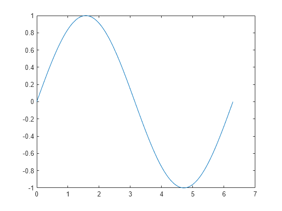
Create x as a vector of linearly spaced values between 0 and 2π. Use an increment of π/100 between the values. Create y as sine values of x. Create a line plot of the data.

x = 0:pi/100:2*pi;
y = sin(x);
plot(x,y)

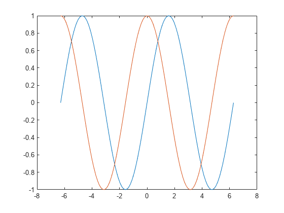
Plot Multiple Lines

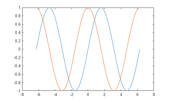
Define x as 100 linearly spaced values between -2π and 2π. Define y1 and y2 as sine and cosine values of x. Create a line plot of both sets of data.

x = linspace(-2*pi,2*pi);
y1 = sin(x);
y2 = cos(x);

figure
plot(x,y1,x,y2)

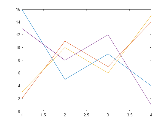
Create Line Plot From Matrix

Define Y as the 4-by-4 matrix returned by the magic function.

Y = 4×4

    16     2     3    13
     5    11    10     8
     9     7     6    12
     4    14    15     1

Create a 2-D line plot of Y. MATLAB® plots each matrix column as a separate line.

Specify Line Style

Plot three sine curves with a small phase shift between each line. Use the default line style for the first line. Specify a dashed line style for the second line and a dotted line style for the third line.

x = 0:pi/100:2*pi;
y1 = sin(x);
y2 = sin(x-0.25);
y3 = sin(x-0.5);

figure
plot(x,y1,x,y2,'--',x,y3,':')

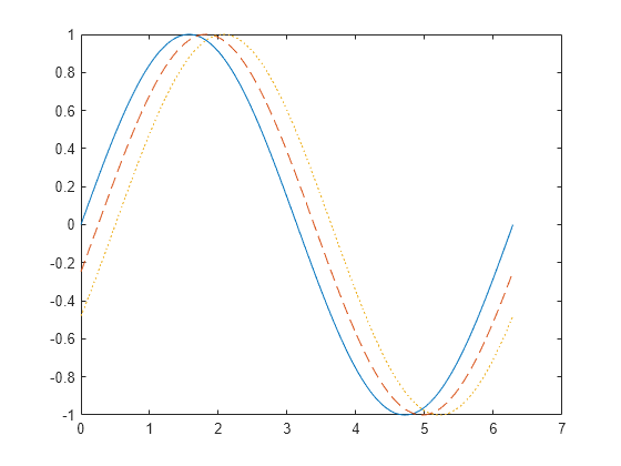
MATLAB® cycles the line color through the default color order.

Specify Line Style, Color, and Marker

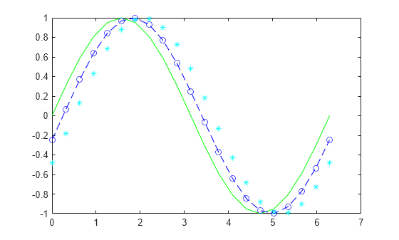
Plot three sine curves with a small phase shift between each line. Use a green line with no markers for the first sine curve. Use a blue dashed line with circle markers for the second sine curve. Use only cyan star markers for the third sine curve.

x = 0:pi/10:2*pi;
y1 = sin(x);
y2 = sin(x-0.25);
y3 = sin(x-0.5);

figure
plot(x,y1,'g',x,y2,'b--o',x,y3,'c*')

Display Markers at Specific Data Points

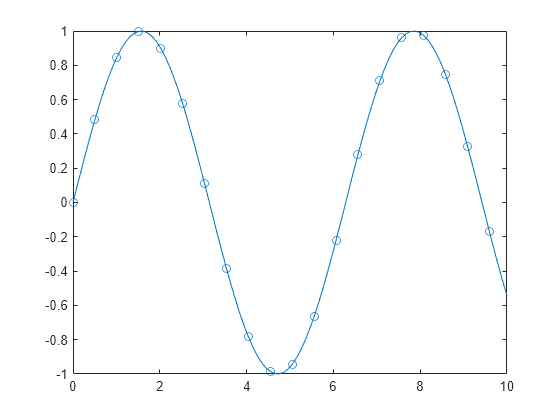
Create a line plot and display markers at every fifth data point by specifying a marker symbol and setting the MarkerIndices property as a name-value pair.

x = linspace(0,10);
y = sin(x);
plot(x,y,'-o','MarkerIndices',1:5:length(y))

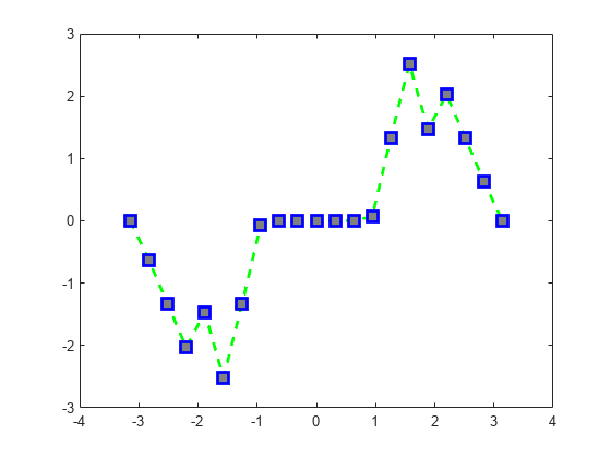
Specify Line Width, Marker Size, and Marker Color

Create a line plot and use the LineSpec option to specify a dashed green line with square markers. Use Name,Value pairs to specify the line width, marker size, and marker colors. Set the marker edge color to blue and set the marker face color using an RGB color value.

x = -pi:pi/10:pi;
y = tan(sin(x)) - sin(tan(x));

figure
plot(x,y,'--gs',...
    'LineWidth',2,...
    'MarkerSize',10,...
    'MarkerEdgeColor','b',...
    'MarkerFaceColor',[0.5,0.5,0.5])

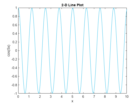
Add Title and Axis Labels

Use the linspace function to define x as a vector of 150 values between 0 and 10. Define y as cosine values of x.

x = linspace(0,10,150);
y = cos(5*x);

Create a 2-D line plot of the cosine curve. Change the line color to a shade of blue-green using an RGB color value. Add a title and axis labels to the graph using the title, xlabel, and ylabel functions.

figure
plot(x,y,'Color',[0,0.7,0.9])

title('2-D Line Plot')
xlabel('x')
ylabel('cos(5x)')

Plot Durations and Specify Tick Format

Define t as seven linearly spaced duration values between 0 and 3 minutes. Plot random data and specify the format of the duration tick marks using the 'DurationTickFormat' name-value pair argument.

t = 0:seconds(30):minutes(3);
y = rand(1,7);

plot(t,y,'DurationTickFormat','mm:ss')

Plot Coordinates from a Table

Since R2022a

A convenient way to plot data from a table is to pass the table to the plot function and specify the variables to plot.

Read weather.csv as a timetable tbl. Then display the first three rows of the table.

tbl = readtimetable("weather.csv");
tbl = sortrows(tbl);
head(tbl,3)

            Time            WindDirection    WindSpeed    Humidity    Temperature    RainInchesPerMinute    CumulativeRainfall    PressureHg    PowerLevel    LightIntensity
    ____________________    _____________    _________    ________    ___________    ___________________    __________________    __________    __________    ______________

    25-Oct-2021 00:00:09         46               1          84          49.2                 0                     0               29.96          4.14             0       
    25-Oct-2021 00:01:09         45             1.6          84          49.2                 0                     0               29.96         4.139             0       
    25-Oct-2021 00:02:09         36             2.2          84          49.2                 0                     0               29.96         4.138             0

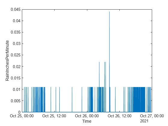
Plot the row times on the x-axis and the RainInchesPerMinute variable on the y-axis. When you plot data from a timetable, the row times are plotted on the x-axis by default. Thus, you do not need to specify the Time variable. Return the Line object as p. Notice that the axis labels match the variable names.

p = plot(tbl,"RainInchesPerMinute");

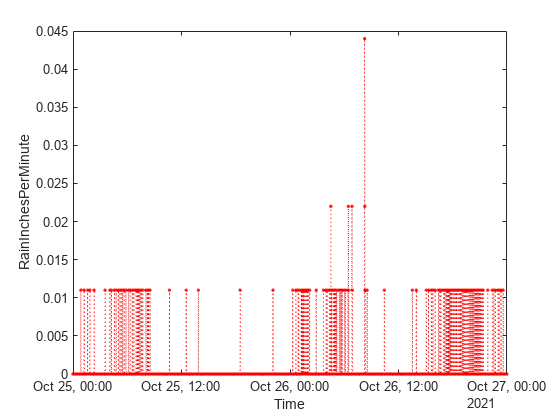
To modify aspects of the line, set the LineStyle, Color, and Marker properties on the Line object. For example, change the line to a red dotted line with point markers.

p.LineStyle = ":";
p.Color = "red";
p.Marker = ".";

Plot Multiple Table Variables on One Axis

Since R2022a

Read weather.csv as a timetable tbl, and display the first few rows of the table.

tbl = readtimetable("weather.csv");
head(tbl,3)

            Time            WindDirection    WindSpeed    Humidity    Temperature    RainInchesPerMinute    CumulativeRainfall    PressureHg    PowerLevel    LightIntensity
    ____________________    _____________    _________    ________    ___________    ___________________    __________________    __________    __________    ______________

    25-Oct-2021 00:00:09         46               1          84          49.2                 0                     0               29.96          4.14             0       
    25-Oct-2021 00:01:09         45             1.6          84          49.2                 0                     0               29.96         4.139             0       
    25-Oct-2021 00:02:09         36             2.2          84          49.2                 0                     0               29.96         4.138             0

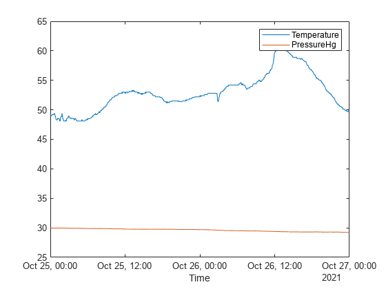
Plot the row times on the x-axis and the Temperature and PressureHg variables on the y-axis. When you plot data from a timetable, the row times are plotted on the x-axis by default. Thus, you do not need to specify the Time variable.

Add a legend. Notice that the legend labels match the variable names.

plot(tbl,["Temperature" "PressureHg"])
legend

Specify Axes for Line Plot

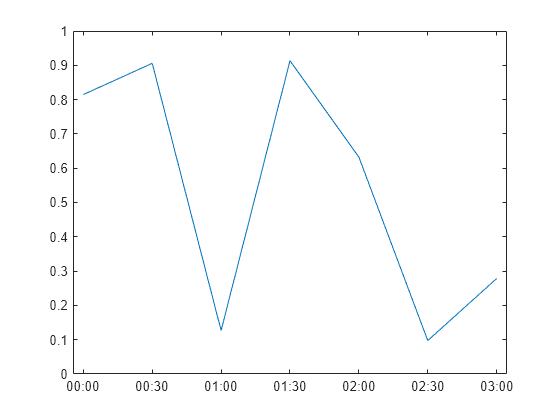
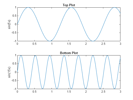
Starting in R2019b, you can display a tiling of plots using the tiledlayout and nexttile functions. Call the tiledlayout function to create a 2-by-1 tiled chart layout. Call the nexttile function to create an axes object and return the object as ax1. Create the top plot by passing ax1 to the plot function. Add a title and y-axis label to the plot by passing the axes to the title and ylabel functions. Repeat the process to create the bottom plot.

% Create data and 2-by-1 tiled chart layout
x = linspace(0,3);
y1 = sin(5*x);
y2 = sin(15*x);
tiledlayout(2,1)

% Top plot
ax1 = nexttile;
plot(ax1,x,y1)
title(ax1,'Top Plot')
ylabel(ax1,'sin(5x)')

% Bottom plot
ax2 = nexttile;
plot(ax2,x,y2)
title(ax2,'Bottom Plot')
ylabel(ax2,'sin(15x)')

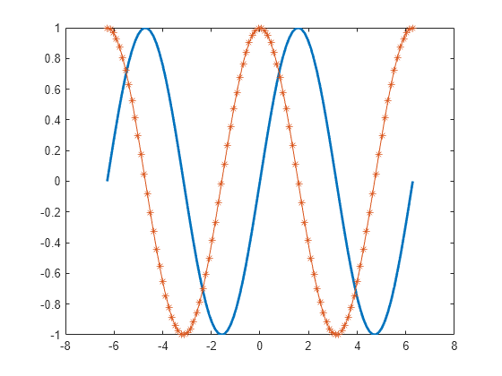
Modify Lines After Creation

Define x as 100 linearly spaced values between -2π and 2π. Define y1 and y2 as sine and cosine values of x. Create a line plot of both sets of data and return the two chart lines in p.

x = linspace(-2*pi,2*pi);
y1 = sin(x);
y2 = cos(x);
p = plot(x,y1,x,y2);

Change the line width of the first line to 2. Add star markers to the second line. Use dot notation to set properties.

p(1).LineWidth = 2;
p(2).Marker = '*';

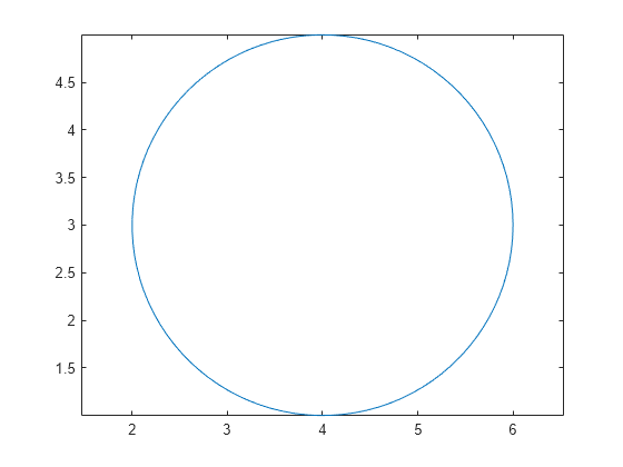
Plot Circle

Plot a circle centered at the point (4,3) with a radius equal to 2. Use axis equal to use equal data units along each coordinate direction.

r = 2;
xc = 4;
yc = 3;

theta = linspace(0,2*pi);
x = r*cos(theta) + xc;
y = r*sin(theta) + yc;
plot(x,y)
axis equal

Input Arguments

collapse all

`X` — x-coordinates
scalar | vector | matrix

x-coordinates, specified as a scalar, vector, or
matrix. The size and shape of X depends on the shape of
your data and the type of plot you want to create. This table describes the
most common situations.

Type of Plot	How to Specify Coordinates
Single point	Specify `X` and `Y` as scalars and include a marker. For example: plot(1,2,"o")
One set of points	Specify `X` and `Y` as any combination of row or column vectors of the same length. For example: plot([1 2 3],[4; 5; 6])
Multiple sets of points (using vectors)	Specify consecutive pairs of `X` and `Y` vectors. For example: plot([1 2 3],[4 5 6],[1 2 3],[7 8 9])
Multiple sets of points (using matrices)	If all the sets share the same x— or y-coordinates, specify the shared coordinates as a vector and the other coordinates as a matrix. The length of the vector must match one of the dimensions of the matrix. For example: plot([1 2 3],[4 5 6; 7 8 9]) If the matrix is square, MATLAB plots one line for each column in the matrix. Alternatively, specify `X` and `Y` as matrices of equal size. In this case, MATLAB plots each column of `Y` against the corresponding column of `X`. For example: plot([1 2 3; 4 5 6],[7 8 9; 10 11 12])

`Y` — y-coordinates
scalar | vector | matrix

y-coordinates, specified as a scalar, vector, or
matrix. The size and shape of Y depends on the shape of
your data and the type of plot you want to create. This table describes the
most common situations.

Type of Plot	How to Specify Coordinates
Single point	Specify `X` and `Y` as scalars and include a marker. For example: plot(1,2,"o")
One set of points	Specify `X` and `Y` as any combination of row or column vectors of the same length. For example: plot([1 2 3],[4; 5; 6]) Alternatively, specify just the y-coordinates. For example: plot([4 5 6])
Multiple sets of points (using vectors)	Specify consecutive pairs of `X` and `Y` vectors. For example: plot([1 2 3],[4 5 6],[1 2 3],[7 8 9])
Multiple sets of points (using matrices)	If all the sets share the same x— or y-coordinates, specify the shared coordinates as a vector and the other coordinates as a matrix. The length of the vector must match one of the dimensions of the matrix. For example: plot([1 2 3],[4 5 6; 7 8 9]) If the matrix is square, MATLAB plots one line for each column in the matrix. Alternatively, specify `X` and `Y` as matrices of equal size. In this case, MATLAB plots each column of `Y` against the corresponding column of `X`. For example: plot([1 2 3; 4 5 6],[7 8 9; 10 11 12])

`LineSpec` — Line style, marker, and color
string | character vector

Line style, marker, and color, specified as a string or character vector containing symbols.
The symbols can appear in any order. You do not need to specify all three
characteristics (line style, marker, and color). For example, if you omit the line style
and specify the marker, then the plot shows only the marker and no line.

Example: "--or" is a red dashed line with circle markers

Line Style	Description	Resulting Line
`"-"`	Solid line
`"--"`	Dashed line
`":"`	Dotted line
`"-."`	Dash-dotted line

Marker	Description	Resulting Marker
`"o"`	Circle
`"+"`	Plus sign
`"*"`	Asterisk
`"."`	Point
`"x"`	Cross
`"_"`	Horizontal line
`"\|"`	Vertical line
`"square"`	Square
`"diamond"`	Diamond
`"^"`	Upward-pointing triangle
`"v"`	Downward-pointing triangle
`">"`	Right-pointing triangle
`"<"`	Left-pointing triangle
`"pentagram"`	Pentagram
`"hexagram"`	Hexagram

Color Name	Short Name	RGB Triplet
`"red"`	`"r"`	`[1 0 0]`
`"green"`	`"g"`	`[0 1 0]`
`"blue"`	`"b"`	`[0 0 1]`
`"cyan"`	`"c"`	`[0 1 1]`
`"magenta"`	`"m"`	`[1 0 1]`
`"yellow"`	`"y"`	`[1 1 0]`
`"black"`	`"k"`	`[0 0 0]`
`"white"`	`"w"`	`[1 1 1]`

`tbl` — Source table
table | timetable

Source table containing the data to plot, specified as a table or a timetable.

`xvar` — Table variables containing x-coordinates
string array | character vector | cell array | pattern | numeric scalar or vector | logical vector | `vartype()`

Table variables containing the x-coordinates, specified
using one of the indexing schemes from the table.

Indexing Scheme	Examples
Variable names: A string, character vector, or cell array. A `pattern` object.	`"A"` or `'A'` — A variable called `A` `["A","B"]` or `{'A','B'}` — Two variables called `A` and `B` `"Var"+digitsPattern(1)` — Variables named `"Var"` followed by a single digit
Variable index: An index number that refers to the location of a variable in the table. A vector of numbers. A logical vector. Typically, this vector is the same length as the number of variables, but you can omit trailing `0` or `false` values.	`3` — The third variable from the table `[2 3]` — The second and third variables from the table `[false false true]` — The third variable
Variable type: A `vartype` subscript that selects variables of a specified type.	`vartype("categorical")` — All the variables containing categorical values

The table variables you specify can contain numeric, categorical,
datetime, or duration values. If xvar and
yvar both specify multiple variables, the number of
variables must be the same.

Example: plot(tbl,["x1","x2"],"y") specifies the table
variables named x1 and x2 for the
x-coordinates.

Example: plot(tbl,2,"y") specifies the second variable
for the x-coordinates.

Example: plot(tbl,vartype("numeric"),"y") specifies all
numeric variables for the x-coordinates.

`yvar` — Table variables containing y-coordinates
string array | character vector | cell array | pattern | numeric scalar or vector | logical vector | `vartype()`

Table variables containing the y-coordinates, specified
using one of the indexing schemes from the table.

Indexing Scheme	Examples
Variable names: A string, character vector, or cell array. A `pattern` object.	`"A"` or `'A'` — A variable called `A` `["A","B"]` or `{'A','B'}` — Two variables called `A` and `B` `"Var"+digitsPattern(1)` — Variables named `"Var"` followed by a single digit
Variable index: An index number that refers to the location of a variable in the table. A vector of numbers. A logical vector. Typically, this vector is the same length as the number of variables, but you can omit trailing `0` or `false` values.	`3` — The third variable from the table `[2 3]` — The second and third variables from the table `[false false true]` — The third variable
Variable type: A `vartype` subscript that selects variables of a specified type.	`vartype("categorical")` — All the variables containing categorical values

The table variables you specify can contain numeric, categorical,
datetime, or duration values. If xvar and
yvar both specify multiple variables, the number of
variables must be the same.

Example: plot(tbl,"x",["y1","y2"]) specifies the table
variables named y1 and y2 for the
y-coordinates.

Example: plot(tbl,"x",2) specifies the second variable
for the y-coordinates.

Example: plot(tbl,"x",vartype("numeric")) specifies all
numeric variables for the y-coordinates.

`ax` — Target axes
`Axes` object | `PolarAxes` object | `GeographicAxes` object

Target axes, specified as an Axes object, a
PolarAxes object, or a
GeographicAxes object. If you do not specify the
axes, MATLAB plots into the current axes or it creates an
Axes object if one does not exist.

To create a polar plot or geographic plot, specify ax
as a PolarAxes or GeographicAxes
object. Alternatively, call the polarplot or geoplot function.

Name-Value Arguments

Specify optional pairs of arguments as
Name1=Value1,...,NameN=ValueN, where Name is
the argument name and Value is the corresponding value.
Name-value arguments must appear after other arguments, but the order of the
pairs does not matter.

Example: plot([0 1],[2 3],LineWidth=2)

Before R2021a, use commas to separate each name and value, and enclose
Name in quotes.

Example: plot([0 1],[2 3],"LineWidth",2)

Note

The properties listed here are only a subset. For a complete list, see
Line Properties.

`Color` — Line color
`[0 0.4470 0.7410]` (default) | RGB triplet | hexadecimal color code | `"r"` | `"g"` | `"b"` | …

Line color, specified as an RGB triplet, a hexadecimal color code, a color name, or a short
name.

For a custom color, specify an RGB triplet or a hexadecimal color code.

An RGB triplet is a three-element row vector whose elements
specify the intensities of the red, green, and blue
components of the color. The intensities must be in the
range [0,1], for example, [0.4 0.6 0.7].
A hexadecimal color code is a character vector or a string
scalar that starts with a hash symbol (#)
followed by three or six hexadecimal digits, which can range
from 0 to F. The
values are not case sensitive. Therefore, the color codes
"#FF8800",
"#ff8800",
"#F80", and
"#f80" are equivalent.

Alternatively, you can specify some common colors by name. This table lists the named color
options, the equivalent RGB triplets, and hexadecimal color codes.

Color Name	Short Name	RGB Triplet	Hexadecimal Color Code	Appearance
`"red"`	`"r"`	`[1 0 0]`	`"#FF0000"`
`"green"`	`"g"`	`[0 1 0]`	`"#00FF00"`
`"blue"`	`"b"`	`[0 0 1]`	`"#0000FF"`
`"cyan"`	`"c"`	`[0 1 1]`	`"#00FFFF"`
`"magenta"`	`"m"`	`[1 0 1]`	`"#FF00FF"`
`"yellow"`	`"y"`	`[1 1 0]`	`"#FFFF00"`
`"black"`	`"k"`	`[0 0 0]`	`"#000000"`
`"white"`	`"w"`	`[1 1 1]`	`"#FFFFFF"`
`"none"`	Not applicable	Not applicable	Not applicable	No color

Here are the RGB triplets and hexadecimal color codes for the default colors MATLAB uses in many types of plots.

RGB Triplet	Hexadecimal Color Code	Appearance
`[0 0.4470 0.7410]`	`"#0072BD"`
`[0.8500 0.3250 0.0980]`	`"#D95319"`
`[0.9290 0.6940 0.1250]`	`"#EDB120"`
`[0.4940 0.1840 0.5560]`	`"#7E2F8E"`
`[0.4660 0.6740 0.1880]`	`"#77AC30"`
`[0.3010 0.7450 0.9330]`	`"#4DBEEE"`
`[0.6350 0.0780 0.1840]`	`"#A2142F"`

Example: "blue"

Example: [0 0 1]

Example: "#0000FF"

Line style, specified as one of the options listed in this table.

Line Style	Description	Resulting Line
`"-"`	Solid line
`"--"`	Dashed line
`":"`	Dotted line
`"-."`	Dash-dotted line
`"none"`	No line	No line

Line width, specified as a positive value in points, where 1 point = 1/72 of an inch. If the
line has markers, then the line width also affects the marker
edges.

The line width cannot be thinner than the width of a pixel. If you set the line width
to a value that is less than the width of a pixel on your system, the line displays as
one pixel wide.

Marker symbol, specified as one of the values listed in this table. By default, the object
does not display markers. Specifying a marker symbol adds markers at each data point or
vertex.

Marker	Description	Resulting Marker
`"o"`	Circle
`"+"`	Plus sign
`"*"`	Asterisk
`"."`	Point
`"x"`	Cross
`"_"`	Horizontal line
`"\|"`	Vertical line
`"square"`	Square
`"diamond"`	Diamond
`"^"`	Upward-pointing triangle
`"v"`	Downward-pointing triangle
`">"`	Right-pointing triangle
`"<"`	Left-pointing triangle
`"pentagram"`	Pentagram
`"hexagram"`	Hexagram
`"none"`	No markers	Not applicable

Indices of data points at which to display markers, specified
as a vector of positive integers. If you do not specify the indices,
then MATLAB displays a marker at every data point.

Note

To see the markers, you must also specify a marker symbol.

Example: plot(x,y,"-o","MarkerIndices",[1 5 10]) displays a circle marker at
the first, fifth, and tenth data points.

Example: plot(x,y,"-x","MarkerIndices",1:3:length(y)) displays a cross
marker every three data points.

Example: plot(x,y,"Marker","square","MarkerIndices",5) displays one square
marker at the fifth data point.

Marker outline color, specified as "auto", an RGB triplet, a
hexadecimal color code, a color name, or a short name. The default value of
"auto" uses the same color as the Color
property.

For a custom color, specify an RGB triplet or a hexadecimal color code.

An RGB triplet is a three-element row vector whose elements
specify the intensities of the red, green, and blue
components of the color. The intensities must be in the
range [0,1], for example, [0.4 0.6 0.7].
A hexadecimal color code is a character vector or a string
scalar that starts with a hash symbol (#)
followed by three or six hexadecimal digits, which can range
from 0 to F. The
values are not case sensitive. Therefore, the color codes
"#FF8800",
"#ff8800",
"#F80", and
"#f80" are equivalent.

Alternatively, you can specify some common colors by name. This table lists the named color
options, the equivalent RGB triplets, and hexadecimal color codes.

Color Name	Short Name	RGB Triplet	Hexadecimal Color Code	Appearance
`"red"`	`"r"`	`[1 0 0]`	`"#FF0000"`
`"green"`	`"g"`	`[0 1 0]`	`"#00FF00"`
`"blue"`	`"b"`	`[0 0 1]`	`"#0000FF"`
`"cyan"`	`"c"`	`[0 1 1]`	`"#00FFFF"`
`"magenta"`	`"m"`	`[1 0 1]`	`"#FF00FF"`
`"yellow"`	`"y"`	`[1 1 0]`	`"#FFFF00"`
`"black"`	`"k"`	`[0 0 0]`	`"#000000"`
`"white"`	`"w"`	`[1 1 1]`	`"#FFFFFF"`
`"none"`	Not applicable	Not applicable	Not applicable	No color

Here are the RGB triplets and hexadecimal color codes for the default colors MATLAB uses in many types of plots.

RGB Triplet	Hexadecimal Color Code	Appearance
`[0 0.4470 0.7410]`	`"#0072BD"`
`[0.8500 0.3250 0.0980]`	`"#D95319"`
`[0.9290 0.6940 0.1250]`	`"#EDB120"`
`[0.4940 0.1840 0.5560]`	`"#7E2F8E"`
`[0.4660 0.6740 0.1880]`	`"#77AC30"`
`[0.3010 0.7450 0.9330]`	`"#4DBEEE"`
`[0.6350 0.0780 0.1840]`	`"#A2142F"`

Marker fill color, specified as "auto", an RGB triplet, a hexadecimal
color code, a color name, or a short name. The "auto" option uses the
same color as the Color property of the parent axes. If you specify
"auto" and the axes plot box is invisible, the marker fill color is
the color of the figure.

For a custom color, specify an RGB triplet or a hexadecimal color code.

An RGB triplet is a three-element row vector whose elements
specify the intensities of the red, green, and blue
components of the color. The intensities must be in the
range [0,1], for example, [0.4 0.6 0.7].
A hexadecimal color code is a character vector or a string
scalar that starts with a hash symbol (#)
followed by three or six hexadecimal digits, which can range
from 0 to F. The
values are not case sensitive. Therefore, the color codes
"#FF8800",
"#ff8800",
"#F80", and
"#f80" are equivalent.

Alternatively, you can specify some common colors by name. This table lists the named color
options, the equivalent RGB triplets, and hexadecimal color codes.

Color Name	Short Name	RGB Triplet	Hexadecimal Color Code	Appearance
`"red"`	`"r"`	`[1 0 0]`	`"#FF0000"`
`"green"`	`"g"`	`[0 1 0]`	`"#00FF00"`
`"blue"`	`"b"`	`[0 0 1]`	`"#0000FF"`
`"cyan"`	`"c"`	`[0 1 1]`	`"#00FFFF"`
`"magenta"`	`"m"`	`[1 0 1]`	`"#FF00FF"`
`"yellow"`	`"y"`	`[1 1 0]`	`"#FFFF00"`
`"black"`	`"k"`	`[0 0 0]`	`"#000000"`
`"white"`	`"w"`	`[1 1 1]`	`"#FFFFFF"`
`"none"`	Not applicable	Not applicable	Not applicable	No color

Here are the RGB triplets and hexadecimal color codes for the default colors MATLAB uses in many types of plots.

RGB Triplet	Hexadecimal Color Code	Appearance
`[0 0.4470 0.7410]`	`"#0072BD"`
`[0.8500 0.3250 0.0980]`	`"#D95319"`
`[0.9290 0.6940 0.1250]`	`"#EDB120"`
`[0.4940 0.1840 0.5560]`	`"#7E2F8E"`
`[0.4660 0.6740 0.1880]`	`"#77AC30"`
`[0.3010 0.7450 0.9330]`	`"#4DBEEE"`
`[0.6350 0.0780 0.1840]`	`"#A2142F"`

Marker size, specified as a positive value in points, where 1 point = 1/72 of an inch.

`DatetimeTickFormat` — Format for `datetime` tick labels
character vector | string

Format for datetime tick labels, specified as the comma-separated pair
consisting of "DatetimeTickFormat" and a character
vector or string containing a date format. Use the letters
A-Z and a-z to construct a
custom format. These letters correspond to the Unicode^® Locale Data Markup Language (LDML) standard for dates. You
can include non-ASCII letter characters such as a hyphen, space, or
colon to separate the fields.

If you do not specify a value for "DatetimeTickFormat", then
plot automatically optimizes and updates the
tick labels based on the axis limits.

Example: "DatetimeTickFormat","eeee, MMMM d, yyyy HH:mm:ss" displays a date
and time such as Saturday, April 19, 2014 21:41:06.

The following table shows several common display formats and
examples of the formatted output for the date, Saturday, April 19,
2014 at 9:41:06 PM in New York City.

Value of `DatetimeTickFormat`	Example
`"yyyy-MM-dd"`	`2014-04-19`
`"dd/MM/yyyy"`	`19/04/2014`
`"dd.MM.yyyy"`	`19.04.2014`
`"yyyy年 MM月 dd日"`	`2014年 04月 19日`
`"MMMM d, yyyy"`	`April 19, 2014`
`"eeee, MMMM d, yyyy HH:mm:ss"`	`Saturday, April 19, 2014 21:41:06`
`"MMMM d, yyyy HH:mm:ss Z"`	`April 19, 2014 21:41:06 -0400`

For a complete list of valid letter identifiers, see the Format property
for datetime arrays.

DatetimeTickFormat is not a chart line property.
You must set the tick format using the name-value pair argument when
creating a plot. Alternatively, set the format using the xtickformat and ytickformat functions.

The TickLabelFormat property of the datetime
ruler stores the format.

`DurationTickFormat` — Format for `duration` tick labels
character vector | string

Format for duration tick labels, specified as the comma-separated pair
consisting of "DurationTickFormat" and a character
vector or string containing a duration format.

If you do not specify a value for "DurationTickFormat", then
plot automatically optimizes and updates the
tick labels based on the axis limits.

To display a duration as a single number that includes a fractional
part, for example, 1.234 hours, specify one of the values in this
table.

Value of `DurationTickFormat`	Description
`"y"`	Number of exact fixed-length years. A fixed-length year is equal to 365.2425 days.
`"d"`	Number of exact fixed-length days. A fixed-length day is equal to 24 hours.
`"h"`	Number of hours
`"m"`	Number of minutes
`"s"`	Number of seconds

Example: "DurationTickFormat","d" displays duration values in terms of
fixed-length days.

To display a duration in the form of a digital timer, specify
one of these values.

"dd:hh:mm:ss"
"hh:mm:ss"
"mm:ss"
"hh:mm"

In addition, you can display up to nine fractional
second digits by appending up to nine S characters.

Example: "DurationTickFormat","hh:mm:ss.SSS" displays the milliseconds of a
duration value to three digits.

DurationTickFormat is not a chart line property.
You must set the tick format using the name-value pair argument when
creating a plot. Alternatively, set the format using the xtickformat and ytickformat functions.

The TickLabelFormat property of the duration
ruler stores the format.

Tips

Use NaN and Inf values
to create breaks in the lines. For example, this code plots the first
two elements, skips the third element, and draws another line using
the last two elements:
plot uses colors and line styles based on the ColorOrder and
LineStyleOrder
properties of the axes. plot cycles through the colors with
the first line style. Then, it cycles through the colors again with each
additional line style.

You can change the colors and the line styles after plotting by
setting the ColorOrder or
LineStyleOrder properties on the axes. You can also
call the colororder function to change the color order for all the axes
in the figure. (since R2019b)

Extended Capabilities

Tall Arrays
Calculate with arrays that have more rows than fit in memory.

Usage notes and limitations:

Supported syntaxes for tall arrays X and Y
are:
- plot(X,Y)
- plot(Y)
- plot(___,LineSpec)
- plot(___,Name,Value)
- plot(ax,___)
X must be in monotonically increasing order.
Categorical inputs are not supported.
Tall inputs must be real column vectors.
With tall arrays, the plot function plots in iterations, progressively adding to the plot as more data is read. During the updates, a progress indicator shows the proportion of data that has been plotted. Zooming and panning is supported during the updating process, before the plot is complete. To stop the update process, press the pause button in the progress indicator.

For more information, see Visualization of Tall Arrays.

GPU Arrays
Accelerate code by running on a graphics processing unit (GPU) using Parallel Computing Toolbox™.

Usage notes and limitations:

This function accepts GPU arrays, but does not run on a GPU.

For more information, see Run MATLAB Functions on a GPU (Parallel Computing Toolbox).

Distributed Arrays
Partition large arrays across the combined memory of your cluster using Parallel Computing Toolbox™.

Usage notes and limitations:

This function operates on distributed arrays, but executes in the client MATLAB.

For more information, see Run MATLAB Functions with Distributed Arrays (Parallel Computing Toolbox).

Version History

Introduced before R2006a

expand all

R2022b: Plots created with tables preserve special characters in axis and legend labels

When you pass a table and one or more variable names to the plot function, the axis and legend labels now display any special characters that are included in the table variable names, such as underscores. Previously, special characters were interpreted as TeX or LaTeX characters.

For example, if you pass a table containing a variable named Sample_Number
to the plot function, the underscore appears in the axis and
legend labels. In R2022a and earlier releases, the underscores are interpreted as
subscripts.

Release	Label for Table Variable `"Sample_Number"`
R2022b
R2022a

To display axis and legend labels with TeX or LaTeX formatting, specify the labels manually.
For example, after plotting, call the xlabel or
legend function with the desired label strings.

xlabel("Sample_Number")
legend(["Sample_Number" "Another_Legend_Label"])

R2022a: Pass tables directly to `plot`

Create plots by passing a table to the plot function followed by the variables you want to plot. When you specify your data as a table, the axis labels and the legend (if present) are automatically labeled using the table variable names.

Источник

plot

Синтаксис

Описание

пример

plot(X,Y) создает 2D график данных в Y по сравнению с соответствующими значениями в X.

Чтобы построить набор координат, соединенных с методической точностью сегменты, задайте X и Y как векторы из той же длины.
Чтобы построить несколько наборов координат на том же наборе осей, задайте по крайней мере один из X или Y как матрица.

plot(X,Y,LineSpec) создает график с помощью заданного стиля линии, маркера и цвета.

пример

plot(X1,Y1,...,Xn,Yn) графики несколько пар x — и y — координируют на том же наборе осей. Используйте этот синтаксис в качестве альтернативы определению координат как матрицы.

пример

plot(X1,Y1,LineSpec1,...,Xn,Yn,LineSpecn) присваивает определенные стили линии, маркеры, и окрашивает к каждому x—y пару. Можно задать LineSpec для некоторого x—y пары и не используют его для других. Например, plot(X1,Y1,'o',X2,Y2) задает маркеры для первого x—y пара, но не для второй пары.

пример

plot(Y) графики Y против неявного набора x — координаты.

Если Y вектор, x — диапазон координат от 1 до length(Y).
Если Y матрица, график содержит одну линию для каждого столбца в Y. x — координирует диапазон от 1 до количества строк в Y.

Если Y содержит комплексные числа, MATLAB^® строит мнимую часть Y по сравнению с действительной частью Y. Если вы задаете оба X и Y, мнимая часть проигнорирована.

plot(Y,LineSpec) задает стиль линии, маркер и цвет.

пример

plot(___,Name,Value) задает Line свойства с помощью одних или нескольких аргументов name-value. Свойства применяются ко всем построенным линиям. Задайте аргументы name-value после всех аргументов в любом из предыдущих синтаксисов. Для списка свойств смотрите Line Properties.

пример

plot(ax,___) отображает график в целевых осях. Задайте оси в качестве первого аргумента в любом из предыдущих синтаксисов.

пример

p = plot(___) возвращает Line возразите или массив Line объекты. Используйте p изменить свойства графика после создания его. Для списка свойств смотрите Line Properties.

Примеры

свернуть все

Построение графика

Создайте x как вектор из линейно распределенных значений между 0 и 2π. Используйте шаг π/100 между значениями. Создайте y как значения синуса x. Постройте график данных.

x = 0:pi/100:2*pi;
y = sin(x);
plot(x,y)

Построение нескольких графиков

Задайте x как 100 линейно распределенных значений между -2π и 2π. Задайте y1 и y2 как синус и значения косинуса xСоздать график для обоих наборов данных.

x = linspace(-2*pi,2*pi);
y1 = sin(x);
y2 = cos(x);

figure
plot(x,y1,x,y2)

Построение графика из матрицы

Задайте Y как матрица 4 на 4, возвращенная magic функция.

Y = 4×4

    16     2     3    13
     5    11    10     8
     9     7     6    12
     4    14    15     1

Постройте 2D график для данных YMATLAB® строит график для каждого столбца матрицы как новый график, новой линией.

Определение стиля линии

Постройте три синусоиды с маленьким сдвигом фазы между каждой линией. Используйте стиль линии по умолчанию для первой линии. Задайте стиль пунктирной линии для второй линии и стиль точечной линии для третьей линии.

x = 0:pi/100:2*pi;
y1 = sin(x);
y2 = sin(x-0.25);
y3 = sin(x-0.5);

figure
plot(x,y1,x,y2,'--',x,y3,':')

MATLAB® циклически повторяет цвет линии через порядок цвета по умолчанию.

Определение стиля линии, цвета и маркера

Постройте три синусоиды с маленьким сдвигом фазы между каждой линией. Используйте зеленую линию без маркеров для первой синусоиды. Используйте синюю пунктирную линию с круговыми маркерами для второй синусоиды. Используйте только голубые маркеры-звездочки для третьей синусоиды.

x = 0:pi/10:2*pi;
y1 = sin(x);
y2 = sin(x-0.25);
y3 = sin(x-0.5);

figure
plot(x,y1,'g',x,y2,'b--o',x,y3,'c*')

Отображение маркеров в определенных точках данных

Постройте график и маркеры отображения в каждой пятой точке данных путем определения символа маркера и установки MarkerIndices свойство как пара «имя-значение».

x = linspace(0,10);
y = sin(x);
plot(x,y,'-o','MarkerIndices',1:5:length(y))

Определение ширины линии, размера маркера и цвета маркера

Постройте график и используйте LineSpec опция, чтобы задать пунктирную зеленую линию с квадратными маркерами. Используйте Name,Value пары, чтобы задать ширину линии, размер маркера и цвета маркера. Установите цвет обводки маркера на синий и выберите цвет поверхности маркера с помощью значения цвета RGB.

x = -pi:pi/10:pi;
y = tan(sin(x)) - sin(tan(x));

figure
plot(x,y,'--gs',...
    'LineWidth',2,...
    'MarkerSize',10,...
    'MarkerEdgeColor','b',...
    'MarkerFaceColor',[0.5,0.5,0.5])

Добавление заголовка и подписей по осям

Используйте linspace функция, чтобы задать x как вектор из 150 значений между 0 и 10. Задайте y как значения косинуса x.

x = linspace(0,10,150);
y = cos(5*x);

Создайте 2D график косинусоиды. Измените цвет линии в оттенок сине-зеленого использования значения цвета RGB. Добавьте заголовок и подписи по осям к графику с помощью titlexlabel, и ylabel функции.

figure
plot(x,y,'Color',[0,0.7,0.9])

title('2-D Line Plot')
xlabel('x')
ylabel('cos(5x)')

Графическое изображение длительности и определение формата метки деления

Задайте t как семь линейно расположил с интервалами duration значения между 0 и 3 минутами. Отобразите случайные данные на графике и задайте формат duration отметки деления с помощью 'DurationTickFormat' аргумент пары «имя-значение».

t = 0:seconds(30):minutes(3);
y = rand(1,7);

plot(t,y,'DurationTickFormat','mm:ss')

Задание осей для графика

Начиная в R2019b, можно отобразить плиточное размещение графиков с помощью tiledlayout и nexttile функции. Вызовите tiledlayout функция, чтобы создать 2 1 мозаичное размещение графика. Вызовите nexttile функция, чтобы создать объект осей и возвратить объект как ax1. Создайте главный график путем передачи ax1 к plot функция. Добавьте заголовок и метку оси Y к графику путем передачи осей title и ylabel функции. Повторите процесс, чтобы создать нижний график.

% Create data and 2-by-1 tiled chart layout
x = linspace(0,3);
y1 = sin(5*x);
y2 = sin(15*x);
tiledlayout(2,1)

% Top plot
ax1 = nexttile;
plot(ax1,x,y1)
title(ax1,'Top Plot')
ylabel(ax1,'sin(5x)')

% Bottom plot
ax2 = nexttile;
plot(ax2,x,y2)
title(ax2,'Bottom Plot')
ylabel(ax2,'sin(15x)')

Изменение линни после ее создания

Задайте x как 100 линейно распределенных значений между -2π и 2π. Задайте y1 и y2 как синус и значения косинуса x. Постройте график обоих наборов данных и возвратите эти две линии на графике в p.

x = linspace(-2*pi,2*pi);
y1 = sin(x);
y2 = cos(x);
p = plot(x,y1,x,y2);

Измените ширину первой линни, задав значение 2. Добавьте маркеры-звездочки во вторую линию. Используйте запись через точку, чтобы установить свойства.

p(1).LineWidth = 2;
p(2).Marker = '*';

Рисование окружности

Постройте круг, сосредоточенный в точке (4,3) с радиусом, равным 2. Используйте axis equal для задания одинаковых маштабов по осям.

r = 2;
xc = 4;
yc = 3;

theta = linspace(0,2*pi);
x = r*cos(theta) + xc;
y = r*sin(theta) + yc;
plot(x,y)
axis equal

Входные параметры

свернуть все

`X` — x — координаты
скаляр | вектор | матрица

x- в виде скаляра, вектора или матрицы. Размер и форма X зависит от формы ваших данных и типа графика, который вы хотите создать. Эта таблица описывает наиболее распространенные ситуации.

Тип графика	Как задать координаты
Одна точка	Задайте `X` и `Y` как скаляры и включают маркер. Например: plot(1,2,'o')
Один набор точек	Задайте `X` и `Y` как любая комбинация строки или вектор-столбцы той же длины. Например: plot([1 2 3],[4; 5; 6])
Несколько наборов точек (использование векторов)	Задайте последовательные пары `X` и `Y` векторы. Например: plot([1 2 3],[4 5 6],[1 2 3],[7 8 9])
Несколько наборов точек (использование матриц)	Если все наборы совместно используют тот же x — или y — координаты, задают разделяемые координаты как вектор и другие координаты как матрица. Длина вектора должна совпадать с одной из размерностей матрицы. Например: plot([1 2 3],[4 5 6; 7 8 9]) Если матрица является квадратной, графики MATLAB одна линия для каждого столбца в матрице. В качестве альтернативы задайте `X` и `Y` как матрицы равного размера. В этом случае, графики MATLAB каждый столбец `Y` против соответствующего столбца `X`. Например: plot([1 2 3; 4 5 6],[7 8 9; 10 11 12])

`Y` — y — координаты
скаляр | вектор | матрица

y- в виде скаляра, вектора или матрицы. Размер и форма Y зависит от формы ваших данных и типа графика, который вы хотите создать. Эта таблица описывает наиболее распространенные ситуации.

Тип графика	Как задать координаты
Одна точка	Задайте `X` и `Y` как скаляры и включают маркер. Например: plot(1,2,'o')
Один набор точек	Задайте `X` и `Y` как любая комбинация строки или вектор-столбцы той же длины. Например: plot([1 2 3],[4; 5; 6]) В качестве альтернативы задайте только y — координаты. Например: plot([4 5 6])
Несколько наборов точек (использование векторов)	Задайте последовательные пары `X` и `Y` векторы. Например: plot([1 2 3],[4 5 6],[1 2 3],[7 8 9])
Несколько наборов точек (использование матриц)	Если все наборы совместно используют тот же x — или y — координаты, задают разделяемые координаты как вектор и другие координаты как матрица. Длина вектора должна совпадать с одной из размерностей матрицы. Например: plot([1 2 3],[4 5 6; 7 8 9]) Если матрица является квадратной, графики MATLAB одна линия для каждого столбца в матрице. В качестве альтернативы задайте `X` и `Y` как матрицы равного размера. В этом случае, графики MATLAB каждый столбец `Y` против соответствующего столбца `X`. Например: plot([1 2 3; 4 5 6],[7 8 9; 10 11 12])

`LineSpec` — Стиль линии, маркер и цвет
вектор символов | строка

Стиль линии, цвет и маркер задается как символ или строка символов. Символы могут появиться в любом порядке. Вы не должны задавать все три характеристики (стиль линии, маркер и цвет). Например, если вы не используете стиль линии и задаете маркер, затем график показывает только маркер и никакую линию.

Пример: '--or' красная пунктирная линия с круговыми маркерами

Стиль линии	Описание	Получившаяся линия
`'-'`	Сплошная линия
`'--'`	Пунктирная линия
`':'`	Пунктирная линия
`'-.'`	Штрих-пунктирная линия

Маркер	Описание	Получившийся маркер
`'o'`	Круг
`'+'`	Знак «плюс»
`'*'`	Звездочка
`'.'`	Точка
`'x'`	Крест
`'_'`	Горизонтальная линия
`'\|'`	Вертикальная линия
`'s'`	Квадрат
`'d'`	Ромб
`'^'`	Треугольник, направленный вверх
`'v'`	Нисходящий треугольник
`'>'`	Треугольник, указывающий вправо
`'<'`	Треугольник, указывающий влево
`'p'`	Пентаграмма
`'h'`	Гексаграмма

Название цвета	Краткое название	Триплет RGB
`'red'`	`'r'`	[1 0 0]
`'green'`	`'g'`	[0 1 0]
`'blue'`	`'b'`	[0 0 1]
`'cyan'`	`'c'`	[0 1 1]
`'magenta'`	`'m'`	[1 0 1]
`'yellow'`	`'y'`	[1 1 0]
`'black'`	`'k'`	[0 0 0]
`'white'`	`'w'`	[1 1 1]

`ax` — Целевые оси
`Axes` возразите | `PolarAxes` возразите | `GeographicAxes` объект

Целевые оси в виде Axes объект, PolarAxes объект или GeographicAxes объект. Если вы не задаете оси, графики MATLAB в текущую систему координат, или это создает Axes возразите, не существуете ли вы.

Чтобы создать полярный график или географический график, задайте ax как PolarAxes или GeographicAxes объект. В качестве альтернативы вызовите polarplot или geoplot функция.

Аргументы name-value

Задайте дополнительные разделенные запятой пары Name,Value аргументы. Name имя аргумента и Value соответствующее значение. Name должен появиться в кавычках. Вы можете задать несколько аргументов в виде пар имен и значений в любом порядке, например: Name1, Value1, ..., NameN, ValueN.

Пример: 'Marker','o','MarkerFaceColor','red'

Свойства линии на графике, перечисленные здесь, являются только подмножеством. Для полного списка смотрите Line Properties.

`Color` ‘LineColor’
[0 0.4470 0.7410] (значение по умолчанию) | триплет RGB | шестнадцатеричный цветовой код | `'r'` | `'g'` | `'b'` | …

Цвет линии в виде триплета RGB, шестнадцатеричного цветового кода, названия цвета или краткого названия.

Для пользовательского цвета задайте триплет RGB или шестнадцатеричный цветовой код.

Триплет RGB представляет собой трехэлементный вектор-строку, элементы которого определяют интенсивность красных, зеленых и синих компонентов цвета. Интенсивность должна быть в области значений [0,1]; например, [0.4 0.6 0.7].
Шестнадцатеричный цветовой код является вектором символов или строковым скаляром, который запускается с символа хеша (#) сопровождаемый тремя или шестью шестнадцатеричными цифрами, которые могут лежать в диапазоне от 0 к F. Значения не являются чувствительными к регистру. Таким образом, цветовые коды '#FF8800', '#ff8800', '#F80', и '#f80' эквивалентны.

Кроме того, вы можете задать имена некоторых простых цветов. Эта таблица приводит опции именованного цвета, эквивалентные триплеты RGB и шестнадцатеричные цветовые коды.

Название цвета	Краткое название	Триплет RGB	Шестнадцатеричный цветовой код	Внешний вид
`'red'`	`'r'`	[1 0 0]	`'#FF0000'`
`'green'`	`'g'`	[0 1 0]	`'#00FF00'`
`'blue'`	`'b'`	[0 0 1]	`'#0000FF'`
`'cyan'`	`'c'`	[0 1 1]	`'#00FFFF'`
`'magenta'`	`'m'`	[1 0 1]	`'#FF00FF'`
`'yellow'`	`'y'`	[1 1 0]	`'#FFFF00'`
`'black'`	`'k'`	[0 0 0]	‘#000000’
`'white'`	`'w'`	[1 1 1]	`'#FFFFFF'`
`'none'`	Не применяется	Не применяется	Не применяется	Нет цвета

Вот являются триплеты RGB и шестнадцатеричные цветовые коды для цветов по умолчанию использованием MATLAB во многих типах графиков.

Триплет RGB	Шестнадцатеричный цветовой код	Внешний вид
[0 0.4470 0.7410]	`'#0072BD'`
[0.8500 0.3250 0.0980]	`'#D95319'`
[0.9290 0.6940 0.1250]	`'#EDB120'`
[0.4940 0.1840 0.5560]	`'#7E2F8E'`
[0.4660 0.6740 0.1880]	`'#77AC30'`
[0.3010 0.7450 0.9330]	`'#4DBEEE'`
[0.6350 0.0780 0.1840]	`'#A2142F'`

Пример: ‘blue’

Пример: [0 0 1]

Пример: '#0000FF'

Стиль линии в виде одной из опций перечислен в этой таблице.

Стиль линии	Описание	Получившаяся линия
`'-'`	Сплошная линия
`'--'`	Пунктирная линия
`':'`	Пунктирная линия
`'-.'`	Штрих-пунктирная линия
`'none'`	Никакая линия	Никакая линия

Ширина линии в виде положительного значения в точках, где 1 точка = 1/72 дюйма. Если у линии есть маркеры, ширина линии также влияет на края маркера.

Ширина линии не может быть более тонкой, чем ширина пикселя. Если вы устанавливаете ширину линии на значение, которое меньше ширины пикселя в вашей системе, отображения линии как один пиксель шириной.

Символ маркера в виде одного из значений перечислен в этой таблице. По умолчанию объект не отображает маркеры. Определение символа маркера добавляет маркеры в каждой точке данных или вершине.

Маркер	Описание	Получившийся маркер
`'o'`	Круг
`'+'`	Знак «плюс»
`'*'`	Звездочка
`'.'`	Точка
`'x'`	Крест
`'_'`	Горизонтальная линия
`'\|'`	Вертикальная линия
`'s'`	Квадрат
`'d'`	Ромб
`'^'`	Треугольник, направленный вверх
`'v'`	Нисходящий треугольник
`'>'`	Треугольник, указывающий вправо
`'<'`	Треугольник, указывающий влево
`'p'`	Пентаграмма
`'h'`	Гексаграмма
`'none'`	Никакие маркеры	Не применяется

Индексы точек данных, в которых можно отобразить маркеры в виде вектора из положительных целых чисел. Если вы не задаете индексы, то MATLAB отображает маркер в каждой точке данных.

Примечание

Чтобы видеть маркеры, необходимо также задать символ маркера.

Пример: plot(x,y,'-o','MarkerIndices',[1 5 10]) отображает круговой маркер во-первых, пятые, и десятые точки данных.

Пример: plot(x,y,'-x','MarkerIndices',1:3:length(y)) отображает перекрестный маркер каждые три точки данных.

Пример: plot(x,y,'Marker','square','MarkerIndices',5) отображения один квадратный маркер в пятой точке данных.

Цвет контура маркера в виде 'auto', триплет RGB, шестнадцатеричный цветовой код, название цвета или краткое название. Значение по умолчанию 'auto' использует тот же цвет в качестве Color свойство.

Для пользовательского цвета задайте триплет RGB или шестнадцатеричный цветовой код.

Триплет RGB представляет собой трехэлементный вектор-строку, элементы которого определяют интенсивность красных, зеленых и синих компонентов цвета. Интенсивность должна быть в области значений [0,1]; например, [0.4 0.6 0.7].
Шестнадцатеричный цветовой код является вектором символов или строковым скаляром, который запускается с символа хеша (#) сопровождаемый тремя или шестью шестнадцатеричными цифрами, которые могут лежать в диапазоне от 0 к F. Значения не являются чувствительными к регистру. Таким образом, цветовые коды '#FF8800', '#ff8800', '#F80', и '#f80' эквивалентны.

Название цвета	Краткое название	Триплет RGB	Шестнадцатеричный цветовой код	Внешний вид
`'red'`	`'r'`	[1 0 0]	`'#FF0000'`
`'green'`	`'g'`	[0 1 0]	`'#00FF00'`
`'blue'`	`'b'`	[0 0 1]	`'#0000FF'`
`'cyan'`	`'c'`	[0 1 1]	`'#00FFFF'`
`'magenta'`	`'m'`	[1 0 1]	`'#FF00FF'`
`'yellow'`	`'y'`	[1 1 0]	`'#FFFF00'`
`'black'`	`'k'`	[0 0 0]	‘#000000’
`'white'`	`'w'`	[1 1 1]	`'#FFFFFF'`
`'none'`	Не применяется	Не применяется	Не применяется	Нет цвета

Триплет RGB	Шестнадцатеричный цветовой код	Внешний вид
[0 0.4470 0.7410]	`'#0072BD'`
[0.8500 0.3250 0.0980]	`'#D95319'`
[0.9290 0.6940 0.1250]	`'#EDB120'`
[0.4940 0.1840 0.5560]	`'#7E2F8E'`
[0.4660 0.6740 0.1880]	`'#77AC30'`
[0.3010 0.7450 0.9330]	`'#4DBEEE'`
[0.6350 0.0780 0.1840]	`'#A2142F'`

Цвет заливки маркера в виде 'auto', триплет RGB, шестнадцатеричный цветовой код, название цвета или краткое название. 'auto' опция использует тот же цвет в качестве Color свойство родительских осей. Если вы задаете 'auto' и поле графика осей невидимо, цвет заливки маркера является цветом фигуры.

Для пользовательского цвета задайте триплет RGB или шестнадцатеричный цветовой код.

Триплет RGB представляет собой трехэлементный вектор-строку, элементы которого определяют интенсивность красных, зеленых и синих компонентов цвета. Интенсивность должна быть в области значений [0,1]; например, [0.4 0.6 0.7].
Шестнадцатеричный цветовой код является вектором символов или строковым скаляром, который запускается с символа хеша (#) сопровождаемый тремя или шестью шестнадцатеричными цифрами, которые могут лежать в диапазоне от 0 к F. Значения не являются чувствительными к регистру. Таким образом, цветовые коды '#FF8800', '#ff8800', '#F80', и '#f80' эквивалентны.

Название цвета	Краткое название	Триплет RGB	Шестнадцатеричный цветовой код	Внешний вид
`'red'`	`'r'`	[1 0 0]	`'#FF0000'`
`'green'`	`'g'`	[0 1 0]	`'#00FF00'`
`'blue'`	`'b'`	[0 0 1]	`'#0000FF'`
`'cyan'`	`'c'`	[0 1 1]	`'#00FFFF'`
`'magenta'`	`'m'`	[1 0 1]	`'#FF00FF'`
`'yellow'`	`'y'`	[1 1 0]	`'#FFFF00'`
`'black'`	`'k'`	[0 0 0]	‘#000000’
`'white'`	`'w'`	[1 1 1]	`'#FFFFFF'`
`'none'`	Не применяется	Не применяется	Не применяется	Нет цвета

Триплет RGB	Шестнадцатеричный цветовой код	Внешний вид
[0 0.4470 0.7410]	`'#0072BD'`
[0.8500 0.3250 0.0980]	`'#D95319'`
[0.9290 0.6940 0.1250]	`'#EDB120'`
[0.4940 0.1840 0.5560]	`'#7E2F8E'`
[0.4660 0.6740 0.1880]	`'#77AC30'`
[0.3010 0.7450 0.9330]	`'#4DBEEE'`
[0.6350 0.0780 0.1840]	`'#A2142F'`

Размер маркера в виде положительного значения в точках, где 1 точка = 1/72 дюйма.

`DatetimeTickFormat` — Формат для `datetime` метки в виде галочки
вектор символов | строка

Формат для datetime метки в виде галочки в виде разделенной запятой пары, состоящей из 'DatetimeTickFormat' и вектор символов или строка, содержащая формат даты. Используйте буквы A-Z и a-z создать пользовательский формат. Эти буквы соответствуют Unicode^® Стандарт языка разметки данных локали (LDML) для дат. Можно включать символы буквы non-ASCII, такие как дефис, пробел или двоеточие, чтобы разделить поля.

Если вы не задаете значение для 'DatetimeTickFormat'то plot автоматически оптимизирует и обновляет метки в виде галочки на основе пределов по осям.

Пример: 'DatetimeTickFormat','eeee, MMMM d, yyyy HH:mm:ss' отображает дату и время, такую как Saturday, April 19, 2014 21:41:06.

Следующая таблица показывает несколько общих форматов отображения и примеров отформатированного вывода для даты, суббота, 19 апреля 2014 в 21:41:06 в Нью-Йорке.

Значение `DatetimeTickFormat`	Пример
`'yyyy-MM-dd'`	2014-04-19
`'dd/MM/yyyy'`	19/04/2014
`'dd.MM.yyyy'`	19.04.2014
`'yyyy年 MM月 dd日'`	2014年 04月 19日
`'MMMM d, yyyy'`	`April 19, 2014`
`'eeee, MMMM d, yyyy HH:mm:ss'`	`Saturday, April 19, 2014 21:41:06`
`'MMMM d, yyyy HH:mm:ss Z'`	`April 19, 2014 21:41:06 -0400`

Для полного списка допустимых идентификаторов буквы смотрите Format свойство для массивов datetime.

DatetimeTickFormat не свойство линии на графике. Необходимо установить формат метки деления с помощью аргумента пары «имя-значение» при создании графика. В качестве альтернативы установите формат с помощью xtickformat и ytickformat функции.

TickLabelFormat свойство линейки datetime хранит формат.

`DurationTickFormat` — Формат для `duration` метки в виде галочки
вектор символов | строка

Формат для duration метки в виде галочки в виде разделенной запятой пары, состоящей из 'DurationTickFormat' и вектор символов или строка, содержащая формат длительности.

Если вы не задаете значение для 'DurationTickFormat'то plot автоматически оптимизирует и обновляет метки в виде галочки на основе пределов по осям.

Чтобы отобразить длительность как, один номер, который включает дробную часть, например, 1,234 часа, задает одно из значений в этой таблице.

Значение `DurationTickFormat`	Описание
`'y'`	Номер точных лет фиксированной длины. Год фиксированной длины равен 365,2425 дням.
`'d'`	Номер точных дней фиксированной длины. День фиксированной длины равен 24 часам.
`'h'`	Номер часов
`'m'`	Номер минут
`'s'`	Номер секунд

Пример: 'DurationTickFormat','d' значения длительности отображений в терминах дней фиксированной длины.

Чтобы отобразить длительность в форме цифрового таймера, задайте одно из этих значений.

'dd:hh:mm:ss'
'hh:mm:ss'
'mm:ss'
'hh:mm'

Кроме того, можно отобразить до девяти цифр доли секунды путем добавления до девяти S ‘characters’.

Пример: 'DurationTickFormat','hh:mm:ss.SSS' отображает миллисекунды значения длительности к трем цифрам.

DurationTickFormat не свойство линии на графике. Необходимо установить формат метки деления с помощью аргумента пары «имя-значение» при создании графика. В качестве альтернативы установите формат с помощью xtickformat и ytickformat функции.

TickLabelFormat свойство линейки длительности хранит формат.

Советы

Используйте NaN и Inf специальные символы, чтобы создать пропуски на линии графика. Например, этот код строит первые два элемента, пропускает третий элемент и проводит другую линию с помощью последних двух элементов:
plot цвета использования и стили линии на основе ColorOrder и LineStyleOrder свойства осей. plot циклы через цвета с первым стилем линии. Затем это циклически повторяется через цвета снова с каждым дополнительным стилем линии.

Начиная в R2019b, можно изменить цвета и стили линии после графического вывода путем установки ColorOrder или LineStyleOrder свойства на осях. Можно также вызвать colororder функционируйте, чтобы изменить последовательность цветов для всех осей на рисунке.

Расширенные возможности

«Высокие» массивы
Осуществление вычислений с массивами, которые содержат больше строк, чем помещается в памяти.

Указания и ограничения по применению:

Поддерживаемые синтаксисы для длинных массивов X и Y :
- plot(X,Y)
- plot(Y)
- plot(___,LineSpec)
- plot(___,Name,Value)
- plot(ax,___)
X должен быть в монотонно увеличивающемся порядке.
Категориальные входные параметры не поддерживаются.
Высокие входные параметры должны быть действительными вектор-столбцами.
С длинными массивами, plot читаются графики функций в итерациях, прогрессивно добавляя к графику как больше данных. Во время обновления, индикатор прогресса показывает долю данных, которые были нанесены. Масштабирование и панорамирование поддерживаются в процессе обновления, до завершения построения. Чтобы остановить процесс обновления, нажмите кнопку паузы в индикаторе хода выполнения.

Для получения дополнительной информации смотрите Визуализацию Длинных массивов.

Массивы графического процессора
Ускорьте код путем работы графического процессора (GPU) с помощью Parallel Computing Toolbox™.

Указания и ограничения по применению:

Эта функция принимает массивы графического процессора, но не работает на графическом процессоре.

Для получения дополнительной информации смотрите функции MATLAB Запуска на графическом процессоре (Parallel Computing Toolbox).

Распределенные массивы
Большие массивы раздела через объединенную память о вашем кластере с помощью Parallel Computing Toolbox™.

Указания и ограничения по применению:

Эта функция работает с распределенными массивами, но выполняет в клиенте MATLAB.

Для получения дополнительной информации смотрите функции MATLAB Запуска с Распределенными Массивами (Parallel Computing Toolbox).

Представлено до R2006a

Источник

GraphPlot Properties

Graph plot appearance and behavior

GraphPlot properties control the appearance and behavior of
plotted graphs. By changing property values, you can modify aspects of the graph display. Use dot
notation to refer to a particular object and property:

G = graph([1 1 1 1 5 5 5 5],[2 3 4 5 6 7 8 9]);
h = plot(G);
c = h.EdgeColor;
h.EdgeColor = 'k';

Nodes

expand all

`NodeColor` — Node color
`[0 0.4470 0.7410]` (default) | RGB triplet | hexadecimal color code | color name | matrix | `'flat'` | `'none'`

Node color, specified as one of these values:

'none' — Nodes are not drawn.
'flat' — Color of each node depends on the value of
NodeCData.
matrix — Each row is an RGB triplet representing the color of one node. The size
of the matrix is numnodes(G)-by-3.

RGB triplet, hexadecimal color code, or color name — All nodes use the specified
color.

RGB triplets and hexadecimal color codes are useful for specifying custom colors.

An RGB triplet is a three-element row vector whose elements specify the
intensities of the red, green, and blue components of the color. The intensities
must be in the range [0,1]; for example,[0.4 0.6 0.7].
A hexadecimal color code is a character vector or a string scalar that starts
with a hash symbol (#) followed by three or six hexadecimal
digits, which can range from 0 to F. The
values are not case sensitive. Thus, the color codes
'#FF8800', '#ff8800',
'#F80', and '#f80' are
equivalent.

Alternatively, you can specify some common colors by name. This table lists the named color options, the equivalent RGB triplets, and hexadecimal color codes.

Color Name	Short Name	RGB Triplet	Hexadecimal Color Code
`"red"`	`"r"`	`[1 0 0]`	`"#FF0000"`
`"green"`	`"g"`	`[0 1 0]`	`"#00FF00"`
`"blue"`	`"b"`	`[0 0 1]`	`"#0000FF"`
`"cyan"`	`"c"`	`[0 1 1]`	`"#00FFFF"`
`"magenta"`	`"m"`	`[1 0 1]`	`"#FF00FF"`
`"yellow"`	`"y"`	`[1 1 0]`	`"#FFFF00"`
`"black"`	`"k"`	`[0 0 0]`	`"#000000"`
`"white"`	`"w"`	`[1 1 1]`	`"#FFFFFF"`

Here are the RGB triplets and hexadecimal color codes for the default colors MATLAB^® uses in many types of plots.

RGB Triplet	Hexadecimal Color Code	Appearance
`[0 0.4470 0.7410]`	`"#0072BD"`
`[0.8500 0.3250 0.0980]`	`"#D95319"`
`[0.9290 0.6940 0.1250]`	`"#EDB120"`
`[0.4940 0.1840 0.5560]`	`"#7E2F8E"`
`[0.4660 0.6740 0.1880]`	`"#77AC30"`
`[0.3010 0.7450 0.9330]`	`"#4DBEEE"`
`[0.6350 0.0780 0.1840]`	`"#A2142F"`

Example: plot(G,'NodeColor','k') creates a graph plot with black
nodes.

`Marker` — Node marker symbol
`'o'` (default) | character vector | cell array | string vector

Node marker symbol, specified as one of the values listed in this table, or as a cell
array or string vector of such values. The default is to use circular markers for the graph
nodes. Specify a cell array of character vectors or string vector to use different markers for
each node.

Marker	Description	Resulting Marker
`"o"`	Circle
`"+"`	Plus sign
`"*"`	Asterisk
`"."`	Point
`"x"`	Cross
`"_"`	Horizontal line
`"\|"`	Vertical line
`"square"`	Square
`"diamond"`	Diamond
`"^"`	Upward-pointing triangle
`"v"`	Downward-pointing triangle
`">"`	Right-pointing triangle
`"<"`	Left-pointing triangle
`"pentagram"`	Pentagram
`"hexagram"`	Hexagram
`"none"`	No markers	Not applicable

Example: '+'

Example: 'diamond'

`MarkerSize` — Node marker size
positive value | vector

Node marker size, specified as a positive value in point units or as a vector of such
values. Specify a vector to use different marker sizes for each node in the graph. The default
value of MarkerSize is 4 for graphs with 100 or fewer nodes, and
2 for graphs with more than 100 nodes.

Example: 10

`NodeCData` — Color data of node markers
vector

Color data of node markers, specified as a vector with length equal to the number of
nodes in the graph. The values in NodeCData map linearly to the colors in
the current colormap, resulting in different colors for each node in the plotted graph.

Edges

expand all

`EdgeColor` — Edge color
`[0 0.4470 0.7410]` (default) | RGB triplet | hexadecimal color code | color name | matrix | `'flat'` | `'none'`

Edge color, specified as one of these values:

'none' — Edges are not drawn.
'flat' — Color of each edge depends on the value of
EdgeCData.
matrix — Each row is an RGB triplet representing the color of one edge. The size
of the matrix is numedges(G)-by-3.

RGB triplet, hexadecimal color code, or color name — All edges use the specified
color.

RGB triplets and hexadecimal color codes are useful for specifying custom colors.

An RGB triplet is a three-element row vector whose elements specify the
intensities of the red, green, and blue components of the color. The intensities
must be in the range [0,1]; for example,[0.4 0.6 0.7].
A hexadecimal color code is a character vector or a string scalar that starts
with a hash symbol (#) followed by three or six hexadecimal
digits, which can range from 0 to F. The
values are not case sensitive. Thus, the color codes
'#FF8800', '#ff8800',
'#F80', and '#f80' are
equivalent.

Alternatively, you can specify some common colors by name. This table lists the named color options, the equivalent RGB triplets, and hexadecimal color codes.

Color Name	Short Name	RGB Triplet	Hexadecimal Color Code
`"red"`	`"r"`	`[1 0 0]`	`"#FF0000"`
`"green"`	`"g"`	`[0 1 0]`	`"#00FF00"`
`"blue"`	`"b"`	`[0 0 1]`	`"#0000FF"`
`"cyan"`	`"c"`	`[0 1 1]`	`"#00FFFF"`
`"magenta"`	`"m"`	`[1 0 1]`	`"#FF00FF"`
`"yellow"`	`"y"`	`[1 1 0]`	`"#FFFF00"`
`"black"`	`"k"`	`[0 0 0]`	`"#000000"`
`"white"`	`"w"`	`[1 1 1]`	`"#FFFFFF"`

Here are the RGB triplets and hexadecimal color codes for the default colors MATLAB uses in many types of plots.

RGB Triplet	Hexadecimal Color Code	Appearance
`[0 0.4470 0.7410]`	`"#0072BD"`
`[0.8500 0.3250 0.0980]`	`"#D95319"`
`[0.9290 0.6940 0.1250]`	`"#EDB120"`
`[0.4940 0.1840 0.5560]`	`"#7E2F8E"`
`[0.4660 0.6740 0.1880]`	`"#77AC30"`
`[0.3010 0.7450 0.9330]`	`"#4DBEEE"`
`[0.6350 0.0780 0.1840]`	`"#A2142F"`

Example: plot(G,'EdgeColor','r') creates a graph plot with red
edges.

`LineStyle` — Line style
`'-'` (default) | `'--'` | `':'` | `'-.'` | `'none'` | cell array | string vector

Line style, specified as one of the line styles listed in this table, or as a cell array
or string vector of such values. Specify a cell array of character vectors or string vector to
use different line styles for each edge.

Character(s)	Line Style	Resulting Line
`'-'`	Solid line
`'--'`	Dashed line
`':'`	Dotted line
`'-.'`	Dash-dotted line
`'none'`	No line	No line

`LineWidth` — Edge line width
`0.5` (default) | positive value | vector

Edge line width, specified as a positive value in point units, or as a vector of such
values. Specify a vector to use a different line width for each edge in the graph.

Example: 0.75

`EdgeAlpha` — Transparency of graph edges
`0.5` (default) | scalar value between `0` and `1` inclusive

Transparency of graph edges, specified as a scalar value between 0 and
1 inclusive. A value of 1 means fully opaque and
0 means completely transparent (invisible).

Example: 0.25

`EdgeCData` — Color data of edge lines
vector

Color data of edge lines, specified as a vector with length equal to the number of edges
in the graph. The values in EdgeCData map linearly to the colors in the
current colormap, resulting in different colors for each edge in the plotted graph.

`ArrowSize` — Arrow size
positive value | vector of positive values

Arrow size, specified as a positive value in point units or as a vector of such values.
As a vector, ArrowSize specifies the size of the arrow for each edge in the
graph. The default value of ArrowSize is 7 for graphs
with 100 or fewer nodes, and 4 for graphs with more than 100 nodes.

ArrowSize only affects directed graphs.

Example: 15

`ArrowPosition` — Position of arrow along edge
`0.5` (default) | scalar | vector

Position of arrow along edge, specified as a value in the range [0 1]
or as a vector of such values with length equal to the number of edges. A value near 0 places
arrows closer to the source node, and a value near 1 places arrows closer to the target node.
The default value is 0.5 so that the arrows are halfway between the source
and target nodes.

ArrowPosition only affects directed graphs.

`ShowArrows` — Toggle display of arrows on directed edges
on/off logical value

Toggle display of arrows on directed edges, specified as 'off' or
'on', or as numeric or logical 1
(true) or 0 (false). A value of
'on' is equivalent to true, and
'off' is equivalent to false. Thus, you can use the
value of this property as a logical value. The value is stored as an on/off logical value of
type matlab.lang.OnOffSwitchState.

For directed graphs the default value is 'on' so that arrows are
displayed, but you can specify a value of 'off' to hide the arrows on the
directed edges. For undirected graphs ShowArrows is always
'off'.

Position

expand all

`XData` — x-coordinate of nodes
vector

Note

XData and YData must be specified together so that
each node has a valid (x,y) coordinate. Optionally, you
can specify ZData for 3-D coordinates.

x-coordinate of nodes, specified as a vector with length equal to the number of nodes in
the graph.

`YData` — y-coordinate of nodes
vector

Note

XData and YData must be specified together so that
each node has a valid (x,y) coordinate. Optionally, you
can specify ZData for 3-D coordinates.

y-coordinate of nodes, specified as a vector with length equal to the number of nodes in
the graph.

`ZData` — z-coordinate of nodes
vector

Note

XData and YData must be specified together so that
each node has a valid (x,y) coordinate. Optionally, you
can specify ZData for 3-D coordinates.

z-coordinate of nodes, specified as a vector with length equal to the number of nodes in
the graph.

Node and Edge Labels

expand all

`NodeLabel` — Node labels
node IDs (default) | vector | cell array of character vectors

Node labels, specified as a numeric vector or cell array of character vectors. The length
of NodeLabel must be equal to the number of nodes in the graph. By default
NodeLabel is a cell array containing the node IDs for the graph
nodes:

For nodes without names (that is, G.Nodes does not contain a
Name variable), the node labels are the values
unique(G.Edges.EndNodes) contained in a cell array.
For named nodes, the node labels are G.Nodes.Name'.

Example: {'A', 'B', 'C'}

Example: [1 2 3]

Example: plot(G,'NodeLabel',G.Nodes.Name) labels the nodes with their
names.

`NodeLabelMode` — Selection mode for node labels
`'auto'` (default) | `'manual'`

Selection mode for node labels, specified as 'auto' (default) or
'manual'. Specify NodeLabelMode as
'auto' to populate NodeLabel with the node IDs for the
graph nodes (numeric node indices or node names). Specifying NodeLabelMode
as 'manual' does not change the values in
NodeLabel.

`NodeLabelColor` — Color of node labels
`[0 0 0]` (default) | RGB triplet | hexadecimal color code | color name | matrix

Node label color, specified as one of these values:

matrix — Each row is an RGB triplet representing the color of one node label.
The size of the matrix is numnodes(G)-by-3.

RGB triplet, hexadecimal color code, or color name — All node labels use the
specified color.

RGB triplets and hexadecimal color codes are useful for specifying custom colors.

An RGB triplet is a three-element row vector whose elements specify the
intensities of the red, green, and blue components of the color. The intensities
must be in the range [0,1]; for example,[0.4 0.6 0.7].
A hexadecimal color code is a character vector or a string scalar that starts
with a hash symbol (#) followed by three or six hexadecimal
digits, which can range from 0 to F. The
values are not case sensitive. Thus, the color codes
'#FF8800', '#ff8800',
'#F80', and '#f80' are
equivalent.

Alternatively, you can specify some common colors by name. This table lists the named color options, the equivalent RGB triplets, and hexadecimal color codes.

Color Name	Short Name	RGB Triplet	Hexadecimal Color Code
`"red"`	`"r"`	`[1 0 0]`	`"#FF0000"`
`"green"`	`"g"`	`[0 1 0]`	`"#00FF00"`
`"blue"`	`"b"`	`[0 0 1]`	`"#0000FF"`
`"cyan"`	`"c"`	`[0 1 1]`	`"#00FFFF"`
`"magenta"`	`"m"`	`[1 0 1]`	`"#FF00FF"`
`"yellow"`	`"y"`	`[1 1 0]`	`"#FFFF00"`
`"black"`	`"k"`	`[0 0 0]`	`"#000000"`
`"white"`	`"w"`	`[1 1 1]`	`"#FFFFFF"`

Here are the RGB triplets and hexadecimal color codes for the default colors MATLAB uses in many types of plots.

RGB Triplet	Hexadecimal Color Code	Appearance
`[0 0.4470 0.7410]`	`"#0072BD"`
`[0.8500 0.3250 0.0980]`	`"#D95319"`
`[0.9290 0.6940 0.1250]`	`"#EDB120"`
`[0.4940 0.1840 0.5560]`	`"#7E2F8E"`
`[0.4660 0.6740 0.1880]`	`"#77AC30"`
`[0.3010 0.7450 0.9330]`	`"#4DBEEE"`
`[0.6350 0.0780 0.1840]`	`"#A2142F"`

Example: plot(G,'NodeLabel',C,'NodeLabelColor','m') creates a graph
plot with magenta node labels.

`EdgeLabel` — Edge labels
`{}` (default) | vector | cell array of character vectors

Edge labels, specified as a numeric vector or cell array of character vectors. The length
of EdgeLabel must be equal to the number of edges in the graph. By default
EdgeLabel is an empty cell array (no edge labels are displayed).

Example: {'A', 'B', 'C'}

Example: [1 2 3]

Example: plot(G,'EdgeLabels',G.Edges.Weight) labels the graph edges
with their weights.

`EdgeLabelMode` — Selection mode for edge labels
`'manual'` (default) | `'auto'`

Selection mode for edge labels, specified as 'manual' (default) or
'auto'. Specify EdgeLabelMode as
'auto' to populate EdgeLabel with the edge weights in
G.Edges.Weight (if available), or the edge indices
G.Edges(k,:) (if no weights are available). Specifying
EdgeLabelMode as 'manual' does not change the values in
EdgeLabel.

`EdgeLabelColor` — Color of edge labels
`[0 0 0]` (default) | RGB triplet | hexadecimal color code | color name | matrix

Edge label color, specified as one of these values:

matrix — Each row is an RGB triplet representing the color of one edge label.
The size of the matrix is numedges(G)-by-3.

RGB triplet, hexadecimal color code, or color name — All edge labels use the
specified color.

RGB triplets and hexadecimal color codes are useful for specifying custom colors.

An RGB triplet is a three-element row vector whose elements specify the
intensities of the red, green, and blue components of the color. The intensities
must be in the range [0,1]; for example,[0.4 0.6 0.7].
A hexadecimal color code is a character vector or a string scalar that starts
with a hash symbol (#) followed by three or six hexadecimal
digits, which can range from 0 to F. The
values are not case sensitive. Thus, the color codes
'#FF8800', '#ff8800',
'#F80', and '#f80' are
equivalent.

Alternatively, you can specify some common colors by name. This table lists the named color options, the equivalent RGB triplets, and hexadecimal color codes.

Color Name	Short Name	RGB Triplet	Hexadecimal Color Code
`"red"`	`"r"`	`[1 0 0]`	`"#FF0000"`
`"green"`	`"g"`	`[0 1 0]`	`"#00FF00"`
`"blue"`	`"b"`	`[0 0 1]`	`"#0000FF"`
`"cyan"`	`"c"`	`[0 1 1]`	`"#00FFFF"`
`"magenta"`	`"m"`	`[1 0 1]`	`"#FF00FF"`
`"yellow"`	`"y"`	`[1 1 0]`	`"#FFFF00"`
`"black"`	`"k"`	`[0 0 0]`	`"#000000"`
`"white"`	`"w"`	`[1 1 1]`	`"#FFFFFF"`

Here are the RGB triplets and hexadecimal color codes for the default colors MATLAB uses in many types of plots.

RGB Triplet	Hexadecimal Color Code	Appearance
`[0 0.4470 0.7410]`	`"#0072BD"`
`[0.8500 0.3250 0.0980]`	`"#D95319"`
`[0.9290 0.6940 0.1250]`	`"#EDB120"`
`[0.4940 0.1840 0.5560]`	`"#7E2F8E"`
`[0.4660 0.6740 0.1880]`	`"#77AC30"`
`[0.3010 0.7450 0.9330]`	`"#4DBEEE"`
`[0.6350 0.0780 0.1840]`	`"#A2142F"`

Example: plot(G,'EdgeLabel',C,'EdgeLabelColor','m') creates a graph
plot with magenta edge labels.

`Interpreter` — Interpretation of text characters
`'tex'` (default) | `'latex'` | `'none'`

Interpretation of text characters, specified as one of these values:

'tex' — Interpret characters using a subset of TeX
markup.
'latex' — Interpret characters using LaTeX markup.
'none' — Display literal characters.

TeX Markup

By default, MATLAB supports a subset of TeX markup. Use TeX markup to add superscripts and
subscripts, modify the font type and color, and include special characters in the
text.

Modifiers remain in effect until the end of the text.
Superscripts and subscripts are an exception because they modify only the next character or the
characters within the curly braces. When you set the interpreter to 'tex',
the supported modifiers are as follows.

Modifier	Description	Example
`^{ }`	Superscript	`'text^{superscript}'`
`_{ }`	Subscript	`'text_{subscript}'`
`bf`	Bold font	`'bf text'`
`it`	Italic font	`'it text'`
`sl`	Oblique font (usually the same as italic font)	`'sl text'`
`rm`	Normal font	`'rm text'`
`fontname{specifier}`	Font name — Replace `specifier` with the name of a font family. You can use this in combination with other modifiers.	`'fontname{Courier} text'`
`fontsize{specifier}`	Font size —Replace `specifier` with a numeric scalar value in point units.	`'fontsize{15} text'`
`color{specifier}`	Font color — Replace `specifier` with one of these colors: `red`, `green`, `yellow`, `magenta`, `blue`, `black`, `white`, `gray`, `darkGreen`, `orange`, or `lightBlue`.	`'color{magenta} text'`
`color[rgb]{specifier}`	Custom font color — Replace `specifier` with a three-element RGB triplet.	`'color[rgb]{0,0.5,0.5} text'`

This table lists the supported special characters for the
'tex' interpreter.

Character Sequence	Symbol	Character Sequence	Symbol	Character Sequence	Symbol
`alpha`	α	`upsilon`	υ	`sim`	~
`angle`	∠	`phi`	ϕ	`leq`	≤
`ast`	`*`	`chi`	χ	`infty`	∞
`beta`	β	`psi`	ψ	`clubsuit`	♣
`gamma`	γ	`omega`	ω	`diamondsuit`	♦
`delta`	δ	`Gamma`	Γ	`heartsuit`	♥
`epsilon`	ϵ	`Delta`	Δ	`spadesuit`	♠
`zeta`	ζ	`Theta`	Θ	`leftrightarrow`	↔
`eta`	η	`Lambda`	Λ	`leftarrow`	←
`theta`	θ	`Xi`	Ξ	`Leftarrow`	⇐
`vartheta`	ϑ	`Pi`	Π	`uparrow`	↑
`iota`	ι	`Sigma`	Σ	`rightarrow`	→
`kappa`	κ	`Upsilon`	ϒ	`Rightarrow`	⇒
`lambda`	λ	`Phi`	Φ	`downarrow`	↓
`mu`	µ	`Psi`	Ψ	`circ`	º
`nu`	ν	`Omega`	Ω	`pm`	±
`xi`	ξ	`forall`	∀	`geq`	≥
`pi`	π	`exists`	∃	`propto`	∝
`rho`	ρ	`ni`	∍	`partial`	∂
`sigma`	σ	`cong`	≅	`bullet`	•
`varsigma`	ς	`approx`	≈	`div`	÷
`tau`	τ	`Re`	ℜ	`neq`	≠
`equiv`	≡	`oplus`	⊕	`aleph`	ℵ
`Im`	ℑ	`cup`	∪	`wp`	℘
`otimes`	⊗	`subseteq`	⊆	`oslash`	∅
`cap`	∩	`in`	∈	`supseteq`	⊇
`supset`	⊃	`lceil`	⌈	`subset`	⊂
`int`	∫	`cdot`	·	`o`	ο
`rfloor`	⌋	`neg`	¬	`nabla`	∇
`lfloor`	⌊	`times`	x	`ldots`	…
`perp`	⊥	`surd`	√	`prime`	´
`wedge`	∧	`varpi`	ϖ		∅
`rceil`	⌉	`rangle`	〉	`mid`	\|
`vee`	∨	`langle`	〈	`copyright`	©

LaTeX Markup

To use LaTeX markup, set the Interpreter property to
'latex'. Use dollar symbols around the text, for example, use
'$int_1^{20} x^2 dx$' for inline mode or '$$int_1^{20} x^2 dx$$' for display mode.

The displayed text uses the default LaTeX font style. The FontName,
FontWeight, and FontAngle properties do not have an
effect. To change the font style, use LaTeX markup.

The maximum size of the text that you can use with the LaTeX interpreter is 1200
characters.

For more information about the LaTeX system, see The LaTeX Project website at https://www.latex-project.org/.

Font

expand all

`NodeFontName` — Font name for node labels
`'Helvetica'` (default) | supported font name | `'FixedWidth'`

Font name for node labels, specified as a supported font name or
'FixedWidth'. For labels to display and print properly, you must choose a
font that your system supports. The default font depends on the specific operating system and
locale. For example, Windows^® and Linux^® systems in English localization use the Helvetica font by default.

To use a fixed-width font that looks good in any locale, specify
'FixedWidth'.

Example: 'Cambria'

`NodeFontSize` — Font size for node labels
`8` (default) | positive number | vector of positive numbers

Font size for node labels, specified as a positive number or a vector of positive
numbers. If NodeFontSize is a vector, then each element specifies the font
size of one node label.

`NodeFontWeight` — Thickness of text in node labels
`'normal'` (default) | `'bold'` | vector | cell array

Thickness of text in node labels, specified as 'normal',
'bold', or as a string vector or cell array of character vectors
specifying 'normal' or 'bold' for each node.

'bold' — Thicker character outlines than
normal
'normal' — Normal weight as defined by the particular font

Not all fonts have a bold font weight.

Data Types: cell | char | string

`NodeFontAngle` — Character slant of text in node labels
`'normal'` (default) | `'italic'` | vector | cell array

Character slant of text in node labels, specified as 'normal',
'italic', or as a string vector or cell array of character vectors
specifying 'normal' or 'italic' for each node.

'italic' — Slanted characters
'normal' — No character slant

Not all fonts have both font styles.

Data Types: cell | char | string

`EdgeFontName` — Font name for edge labels
`'Helvetica'` (default) | supported font name | `'FixedWidth'`

Font name for edge labels, specified as a supported font name or
'FixedWidth'. For labels to display and print properly, you must choose a
font that your system supports. The default font depends on the specific operating system and
locale. For example, Windows and Linux systems in English localization use the Helvetica font by default.

To use a fixed-width font that looks good in any locale, specify
'FixedWidth'.

Example: 'Cambria'

`EdgeFontSize` — Font size for edge labels
`8` (default) | positive number | vector of positive numbers

Font size for edge labels, specified as a positive number or a vector of positive
numbers. If EdgeFontSize is a vector, then each element specifies the font
size of one edge label.

`EdgeFontWeight` — Thickness of text in edge labels
`'normal'` (default) | `'bold'` | vector | cell array

Thickness of text in edge labels, specified as 'normal',
'bold', or as a string vector or cell array of character vectors
specifying 'normal' or 'bold' for each edge.

'bold' — Thicker character outlines than
normal
'normal' — Normal weight as defined by the particular font

Not all fonts have a bold font weight.

Data Types: cell | char | string

`EdgeFontAngle` — Character slant of text in edge labels
`'normal'` (default) | `'italic'` | vector | cell array

Character slant of text in edge labels, specified as 'normal',
'italic', or as a string vector or cell array of character vectors
specifying 'normal' or 'italic' for each edge.

'italic' — Slanted characters
'normal' — No character slant

Not all fonts have both font styles.

Data Types: cell | char | string

Legend

expand all

`DisplayName` — Text used by legend
`''` (default) | character vector

Text used by the legend, specified as a character vector. The text appears next to an
icon of the GraphPlot.

Example: 'Text Description'

For multiline text, create the character vector using sprintf with the
new line character n.

Example: sprintf('line onenline two')

Alternatively, you can specify the legend text using the legend function.

If you specify the text as an input argument to the legend function, then the legend uses the specified text and sets the
DisplayName property to the same value.
If you do not specify the text as an input argument to the legend function, then the legend uses the text in the
DisplayName property. If the DisplayName property
does not contain any text, then the legend generates a character vector. The character
vector has the form 'dataN', where N is the number
assigned to the GraphPlot object based on its location in the list of
legend entries.

If you edit interactively the character vector in an existing legend, then MATLAB updates the DisplayName property to the edited character
vector.

`Annotation` — Legend icon display style
`Annotation` object

This property is read-only.

Legend icon display style, returned as an Annotation object. Use this
object to include or exclude the GraphPlot from a legend.

Query the Annotation property to get the
Annotation object.
Query the LegendInformation property of the
Annotation object to get the LegendEntry
object.
Specify the IconDisplayStyle property of the
LegendEntry object to one of these values:
- 'on' — Include the GraphPlot object in
  the legend as one entry (default).
- 'off' — Do not include the GraphPlot
  object in the legend.
- 'children' — Include only children of the GraphPlot object as separate entries in the legend.

If a legend already exists and you change the
IconDisplayStyle setting, then you must call legend to
update the display.

Interactivity

expand all

State of visibility, specified as 'on' or 'off', or as
numeric or logical 1 (true) or
0 (false). A value of 'on'
is equivalent to true, and 'off' is equivalent to
false. Thus, you can use the value of this property as a logical
value. The value is stored as an on/off logical value of type matlab.lang.OnOffSwitchState.

'on' — Display the object.
'off' — Hide the object without deleting it. You
still can access the properties of an invisible object.

`DataTipTemplate` — Data tip content
`DataTipTemplate` object

Data tip content, specified as a DataTipTemplate object. You can
control the content that appears in a data tip by modifying the properties of the
underlying DataTipTemplate object. For a list of properties, see
DataTipTemplate Properties.

For an example of modifying data tips, see Create Custom Data Tips.

Note

The DataTipTemplate object is not returned by
findobj or findall, and it is not
copied by copyobj.

Context menu, specified as a ContextMenu object. Use this property
to display a context menu when you right-click the object. Create the context menu using
the uicontextmenu function.

Note

If the PickableParts property is set to
'none' or if the HitTest property is set
to 'off', then the context menu does not appear.

Selection state, specified as 'on' or 'off', or as
numeric or logical 1 (true) or
0 (false). A value of 'on'
is equivalent to true, and 'off' is equivalent to
false. Thus, you can use the value of this property as a logical
value. The value is stored as an on/off logical value of type matlab.lang.OnOffSwitchState.

'on' — Selected. If you click the object when in
plot edit mode, then MATLAB sets its Selected property to
'on'. If the SelectionHighlight
property also is set to 'on', then MATLAB displays selection handles around the object.
'off' — Not selected.

Display of selection handles when selected, specified as 'on' or
'off', or as numeric or logical 1
(true) or 0 (false). A
value of 'on' is equivalent to true, and 'off' is
equivalent to false. Thus, you can use the value of this property as
a logical value. The value is stored as an on/off logical value of type matlab.lang.OnOffSwitchState.

'on' — Display selection handles when the
Selected property is set to
'on'.
'off' — Never display selection handles, even
when the Selected property is set to
'on'.

Callbacks

expand all

`ButtonDownFcn` — Mouse-click callback
`''` (default) | function handle | cell array | character vector

Mouse-click callback, specified as one of these values:

Function handle
Cell array containing a function handle and additional arguments
Character vector that is a valid MATLAB command or function, which is evaluated in the base workspace (not
recommended)

Use this property to execute code when you click the GraphPlot. If you
specify this property using a function handle, then MATLAB passes two arguments to the callback function when executing the callback:

The GraphPlot object — You can access properties of the
GraphPlot object from within the callback function.
Event data — This argument is empty for this property. Replace it with the
tilde character (~) in the function definition to indicate that this
argument is not used.

For more information on how to use function handles to define callback
functions, see Create Callbacks for Graphics Objects.

Note

If the PickableParts property is set to 'none'
or if the HitTest property is set to 'off', then this
callback does not execute.

Example: @myCallback

Example: {@myCallback,arg3}

`CreateFcn` — Creation callback
`''` (default) | function handle | cell array | character vector

Creation callback, specified as one of these values:

Function handle
Cell array containing a function handle and additional arguments
Character vector that is a valid MATLAB command or function, which is evaluated in the base workspace (not
recommended)

Use this property to execute code when you create the GraphPlot.
Setting the CreateFcn property on an existing GraphPlot
has no effect. You must define a default value for this property, or define this property
using a Name,Value pair during GraphPlot creation.
MATLAB executes the callback after creating the GraphPlot and setting
all of its properties.

If you specify this callback using a function handle, then MATLAB passes two arguments to the callback function when executing the callback:

The GraphPlot object — You can access properties of the
GraphPlot object from within the callback function. You also can access
the GraphPlot object through the CallbackObject
property of the root, which can be queried using the gcbo
function.
Event data — This argument is empty for this property. Replace it with the
tilde character (~) in the function definition to indicate that this
argument is not used.

For more information on how to use function handles to define callback
functions, see Create Callbacks for Graphics Objects.

Example: @myCallback

Example: {@myCallback,arg3}

`DeleteFcn` — Deletion callback
`''` (default) | function handle | cell array | character vector

Deletion callback, specified as one of these values:

Function handle
Cell array containing a function handle and additional arguments
Character vector that is a valid MATLAB command or function, which is evaluated in the base workspace (not
recommended)

Use this property to execute code when you delete the GraphPlot.
MATLAB executes the callback before destroying the GraphPlot so that
the callback can access its property values.

If you specify this callback using a function handle, then MATLAB passes two arguments to the callback function when executing the callback:

The GraphPlot object — You can access properties of the
GraphPlot object from within the callback function. You also can access
the GraphPlot object through the CallbackObject
property of the root, which can be queried using the gcbo
function.
Event data — This argument is empty for this property. Replace it with the
tilde character (~) in the function definition to indicate that this
argument is not used.

For more information on how to use function handles to define callback
functions, see Create Callbacks for Graphics Objects.

Example: @myCallback

Example: {@myCallback,arg3}

Callback Execution Control

expand all

Callback interruption, specified as 'on' or 'off', or as
numeric or logical 1 (true) or
0 (false). A value of 'on'
is equivalent to true, and 'off' is equivalent to
false. Thus, you can use the value of this property as a logical
value. The value is stored as an on/off logical value of type matlab.lang.OnOffSwitchState.

This property determines if a running callback can be interrupted. There are two callback
states to consider:

The running callback is the currently executing
callback.
The interrupting callback is a callback that tries
to interrupt the running callback.

MATLAB determines callback interruption behavior whenever it executes a command that
processes the callback queue. These commands include drawnow, figure, uifigure, getframe, waitfor, and pause.

If the running callback does not contain one of these commands, then no interruption
occurs. MATLAB first finishes executing the running callback, and later executes the
interrupting callback.

If the running callback does contain one of these commands, then the
Interruptible property of the object that owns the running
callback determines if the interruption occurs:

If the value of Interruptible is
'off', then no interruption occurs. Instead, the
BusyAction property of the object that owns the
interrupting callback determines if the interrupting callback is discarded or
added to the callback queue.
If the value of Interruptible is 'on',
then the interruption occurs. The next time MATLAB processes the callback queue, it stops the execution of the
running callback and executes the interrupting callback. After the interrupting
callback completes, MATLAB then resumes executing the running callback.

Note

Callback interruption and execution behave differently in these situations:

If the interrupting callback is a DeleteFcn,
CloseRequestFcn, or
SizeChangedFcn callback, then the interruption
occurs regardless of the Interruptible property
value.
If the running callback is currently executing the
waitfor function, then the interruption occurs
regardless of the Interruptible property
value.
If the interrupting callback is owned by a Timer object, then the callback executes according to
schedule regardless of the Interruptible property
value.

Note

When an interruption occurs, MATLAB does not save the state of properties or the display. For example, the
object returned by the gca or gcf command might change when
another callback executes.

`BusyAction` — Callback queuing
`'queue'` (default) | `'cancel'`

Callback queuing specified as 'queue' or 'cancel'.
The BusyAction property determines how MATLAB handles the execution of interrupting callbacks.

Note

There are two callback states to consider:

The running callback is the currently executing callback.
The interrupting callback is a callback that tries to interrupt
the running callback.

Whenever MATLAB invokes a callback, that callback attempts to interrupt a running callback. The
Interruptible property of the object owning the running callback
determines if interruption is allowed. If interruption is not allowed, then the
BusyAction property of the object owning the interrupting callback
determines if it is discarded or put in the queue.

If the ButtonDownFcn callback of the GraphPlot tries
to interrupt a running callback that cannot be interrupted, then the
BusyAction property determines if it is discarded or put in the queue.
Specify the BusyAction property as one of these values:

'queue' — Put the interrupting callback in a queue to be
processed after the running callback finishes execution. This is the default
behavior.
'cancel' — Discard the interrupting callback.

`PickableParts` — Ability to capture mouse clicks
`'visible'` (default) | `'none'`

Ability to capture mouse clicks, specified as one of these values:

'visible' — Can capture mouse clicks only when visible. The
Visible property must be set to 'on'. The
HitTest property determines if the GraphPlot
responds to the click or if an ancestor does.
'none' — Cannot capture mouse clicks. Clicking the GraphPlot passes the click to the object below it in the current view of the
figure window. The HitTest property of the GraphPlot
has no effect.

Response to captured mouse clicks, specified as 'on' or
'off', or as numeric or logical 1
(true) or 0 (false). A
value of 'on' is equivalent to true, and 'off' is
equivalent to false. Thus, you can use the value of this property as
a logical value. The value is stored as an on/off logical value of type matlab.lang.OnOffSwitchState.

'on' — Trigger the
ButtonDownFcn callback of the GraphPlot object. If you have
defined the ContextMenu property, then invoke the
context menu.
'off' — Trigger the callbacks for the nearest
ancestor of the GraphPlot object that has one of these:
- HitTest property set to
  'on'
- PickableParts property set to a value that
  enables the ancestor to capture mouse clicks

Note

The PickableParts property determines if
the GraphPlot object can capture
mouse clicks. If it cannot, then the HitTest property
has no effect.

This property is read-only.

Deletion status, returned as an on/off logical value of type matlab.lang.OnOffSwitchState.

MATLAB sets the BeingDeleted property to
'on' when the DeleteFcn callback begins
execution. The BeingDeleted property remains set to
'on' until the component object no longer exists.

Check the value of the BeingDeleted property to verify that the object is not about to be deleted before querying or modifying it.

Parent/Child

expand all

`Parent` — Parent of GraphPlot
axes object | group object | transform object

Parent of GraphPlot, specified as an axes, group, or transform
object.

Children, returned as an empty GraphicsPlaceholder array or a
DataTip object array. Use this property to view a list of data tips
that are plotted on the chart.

You cannot add or remove children using the Children property. To add a
child to this list, set the Parent property of the
DataTip object to the chart object.

`HandleVisibility` — Visibility of object handle
`'on'` (default) | `'off'` | `'callback'`

Visibility of GraphPlot object handle in the
Children property of the parent, specified as one of these values:

'on' — The GraphPlot object handle is
always visible.
'off' — The GraphPlot object handle is
invisible at all times. This option is useful for preventing unintended changes to the UI
by another function. Set the HandleVisibility to
'off' to temporarily hide the handle during the execution of that
function.
'callback' — The GraphPlot object handle
is visible from within callbacks or functions invoked by callbacks, but not from within
functions invoked from the command line. This option blocks access to the GraphPlot at the command-line, but allows callback functions to access it.

If the GraphPlot object is not listed in the
Children property of the parent, then functions that obtain object handles
by searching the object hierarchy or querying handle properties cannot return it. This
includes get, findobj, gca, gcf, gco, newplot, cla, clf, and close.

Hidden object handles are still valid. Set the root
ShowHiddenHandles property to 'on' to list all object
handles regardless of their HandleVisibility property setting.

Identifiers

expand all

`Type` — Type of graphics object
`'graphplot'`

This property is read-only.

Type of graphics object, returned as 'graphplot'. Use this property to
find all objects of a given type within a plotting hierarchy, such as searching for the type
using findobj.

`Tag` — Tag to associate with GraphPlot
`''` (default) | character vector

Tag to associate with the GraphPlot, specified as a character vector.
Tags provide a way to identify graphics objects. Use this property to find all objects with a
specific tag within a plotting hierarchy, for example, searching for the tag using findobj.

Example: 'January Data'

Data Types: char

`UserData` — Data to associate with GraphPlot
`[]` (default) | scalar, vector, or matrix | cell array | character array | table | structure

Data to associate with the GraphPlot object, specified as a scalar,
vector, matrix, cell array, character array, table, or structure. MATLAB does not use this data.

To associate multiple sets of data or to attach a field name to the data, use the
getappdata and setappdata functions.

Example: 1:100

Version History

Introduced in R2015b

expand all

R2020a: `UIContextMenu` property is not recommended

Starting in R2020a, using the UIContextMenu property to assign a
context menu to a graphics object or UI component is not recommended. Use the
ContextMenu property instead. The property values are the same.

There are no plans to remove support for the UIContextMenu property at
this time. However, the UIContextMenu property no longer appears in the
list returned by calling the get function on a graphics object or UI
component.

Источник

Как менять цвет графика в матлаб

Пакет MatLab позволяет отображать графики с разным цветом и типом линий, показывать или скрывать сетку на графике, выполнять подпись осей и графика в целом, создавать легенду и многое другое. В данном параграфе рассмотрим наиболее важные функции, позволяющие делать такие оформления на примере двумерных графиков.

Функция plot() позволяет менять цвет и тип отображаемой линии. Для этого, используются дополнительные параметры, которые записываются следующим образом:

plot(<x>, <y>, <’цвет линии, тип линии, маркер точек’>);

Обратите внимание, что третий параметр записывается в апострофах и имеет обозначения, приведенные в таблицах 3.1-3.3. Маркеры, указанные ниже записываются подряд друг за другом, например,

‘ko’ – на графике отображает черными кружками точки графика,
‘ko-‘ – рисует график черной линией и проставляет точки в виде кружков.

Ниже показаны примеры записи функции plot() с разным набором маркеров.

x = 0:0.1:2*pi;
y = sin(x);

subplot(2,2,1); plot(x,y,’r-‘);
subplot(2,2,2); plot(x,y,’r-‘,x,y,’ko’);
subplot(2,2,3); plot(y,’b—‘);
subplot(2,2,4); plot(y,’b—+’);

Результат работы фрагмента программы приведен на рис. 3.7. Представленный пример показывает, каким образом можно комбинировать маркеры для достижения требуемого результата. А на рис. 3.7 наглядно видно к каким визуальным эффектам приводят разные маркеры, используемые в программе. Следует особо отметить, что в четвертой строчке программы по сути отображаются два графика: первый рисуется красным цветом и непрерывной линией, а второй черными кружками заданных точек графика. Остальные варианты записи маркеров очевидны.

Рис. 3.7. Примеры отображения графиков с разными типами маркеров

Из примеров рис. 3.7 видно, что масштаб графиков по оси Ox несколько больше реальных значений. Дело в том, что система MatLab автоматически масштабирует систему координат для полного представления данных. Однако такая автоматическая настройка не всегда может удовлетворять интересам пользователя. Иногда требуется выделить отдельный фрагмент графика и только его показать целиком. Для этого используется функция axis() языка MatLab, которая имеет следующий синтаксис:

axis( [ xmin, xmax, ymin, ymax ] ),

где название указанных параметров говорят сами за себя.

Воспользуемся данной функцией для отображения графика функции синуса в пределах от 0 до :

x = 0:0.1:2*pi;
y = sin(x);

subplot(1,2,1);
plot(x,y);
axis([0 2*pi -1 1]);

subplot(1,2,2);
plot(x,y);
axis([0 pi 0 1]);

Из результата работы программы (рис. 3.8) видно, что несмотря на то, что функция синуса задана в диапазоне от 0 до , с помощью функции axis() можно отобразить как весь график, так и его фрагмент в пределах от 0 до .

Рис. 3.8. Пример работы функции axis()

В заключении данного параграфа рассмотрим возможности создания подписей графиков, осей и отображения сетки на графике. Для этого используются функции языка MatLab, перечисленные в табл. 3.4.

Рассмотрим работу данных функций в следующем примере:

x = 0:0.1:2*pi;
y = sin(x);

plot(x,y);
axis([0 2*pi -1 1]);
grid on;
title(‘The graphic of sin(x) function’);
xlabel(‘The coordinate of Ox’);
ylabel(‘The coordinate of Oy’);
text(3.05,0.16,’leftarrow sin(x)’);

Из результата работы данной программы, представленного на рис. 3.9, видно каким образом работают функции создания подписей на графике, а также отображение сетки графика.

Таким образом, используя описанный набор функций и параметров, можно достичь желаемого способа оформления графиков в системе MatLab.

Рис. 3.9. Пример работы функций оформления графика

Копирование информации со страницы разрешается только с указанием ссылки на данный сайт

Настраиваем графики в MATLAB

Команда plot имеет множество настроек, которые определяют цвет, толщину и стиль линий, а также параметры маркеров на ваших графиках. Предлагаемые по умолчанию настройки неплохо смотрятся на экране настольного компьютера, но в презентациях требуются более жирные линии и более заметный шрифт. Рассмотрим как этого добиться с помощью настроек plot .

Данные

Упражняться будем на примере обычной синусоиды.

Обратите внимание на первую строку. В ней не только очищается память (Workspace) и командное окно MATLAB, но и закрываются все открытые ранее графические окна ( close all ). Очень полезно, чтобы не запутаться в старых и новых версиях рисунков.

Исходный график

Настроим график

А теперь давайте увеличим толщину линии, изменим ее цвет на красный и сделаем на ней маркеры в виде закрашенных красным кружков с черным контуром. Кроме того, сделаем размер рисунков равным 10х7.5 дюймов (4:3).

Настроим подписи к осям

На подписях к осям координат сделаем более крупный шрифт — 12 пт. Подпись к оси Х выполним полужирным шрифтом, а к оси Y — курсивом, вдобавок изменив цвет шрифта на синий.

Настроим все текстовые свойства рисунка.

Да, но теперь стиль цифр вдоль осей координат отличается от стиля подписей. А если к тому же у вас на одном рисунке размещено несколько координатных осей и несколько графиков. Нельзя ли выделить сразу все текстовые объекты и изменить их свойства? Конечно можно. Более того, аналогично можно выделить все линии и изменить их настройки. Вот как это делается.

Вначале выделим все объекты. Затем среди них выделим оси, линии и текстовые объекты. И, наконец, установим свойства объектов.

Дмитрий Храмов
Компьютерное моделирование и все, что с ним связано: сбор данных, их анализ, разработка математических моделей, софт для моделирования, визуализации и оформления публикаций. Ну и за жизнь немного.

Colors in MATLAB plots

for more in-depth explanations and fancier coloring, to name just two sources.

Default Colors in 2D Graphs

The default colors used in MATLAB changed in R2014b version. Here are the colors, in order, and their MATLAB RGB triplet.

Current color	Old color
[0, 0.4470, 0.7410]	[0, 0, 1]
[0.8500, 0.3250, 0.0980]	[0, 0.5, 0]
[0.9290, 0.6940, 0.1250]	[1, 0, 0]
[0.4940, 0.1840, 0.5560]	[0, 0.75, 0.75]
[0.4660, 0.6740, 0.1880]	[0.75, 0, 0.75]
[0.3010, 0.7450, 0.9330]	[0.75, 0.75, 0]
[0.6350, 0.0780, 0.1840]	[0.25, 0.25, 0.25]

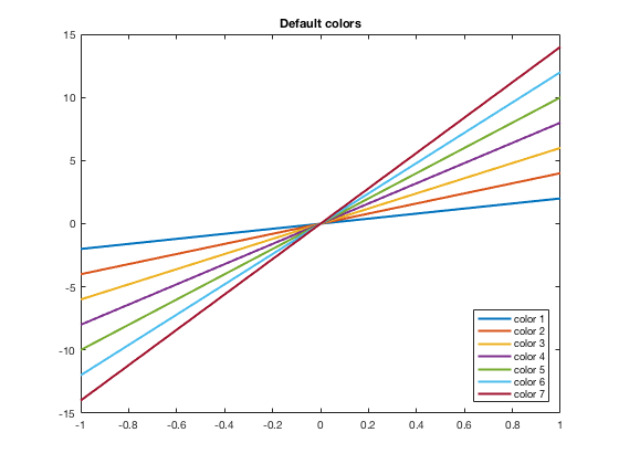
Another thing that changed starting in the R2014b version is that the hold on and hold off automatically cycles through the colors. In the past, each new plot command would start with the first color (blue) and you would have to manually change the color. Now it will automatically move to the next color(s). See below for how to manually adjust the colors.

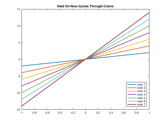
Default Colors in 3D Graphs

If using mesh(x,y,z), to change the look of it you would want to change ‘EdgeColor’. Note that the name of this colormap is «parula» while previous to R2014b, it was «jet»

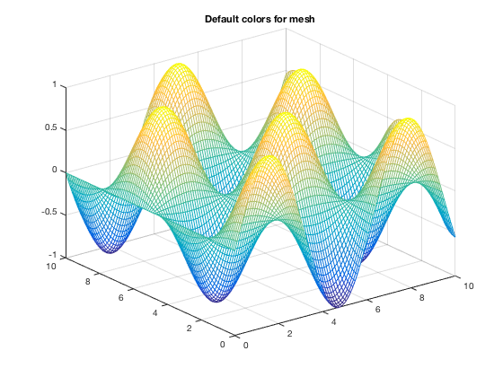
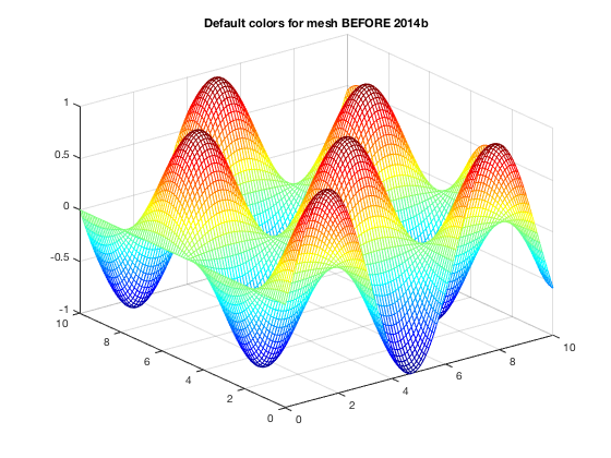
Using Basic Colors in Graphs

The eight basic colors are known by either their short name or long name (RGB triplets are also included).

Long Name	Short Name	RGB Triplet
blue	b	[0,0,1]
black	k	[0,0,0]
red	r	[1,0,0]
green	g	[0,1,0]
yellow	y	[1,1,0]
cyan	c	[0,1,1]
magenta	m	[1,0,1]
white	w	[1,1,1]

Example of how to change the color using short names is below. You can easily do the same thing using the long names.

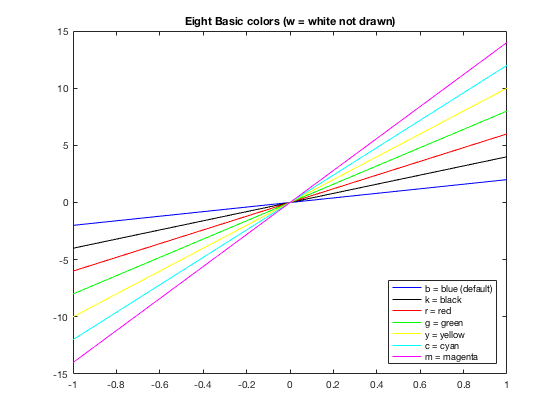
Changing Colors

Many times you want to have more control of what colors are used. For example, I may want some data points drawn in the same color as the curve. Or I have a piece-wise graph that I want to have all the same color. There are several ways to do this. One is to use the default colors and «resetting» the order, which is shown here. Others involve using the RGB triplet (see next section).

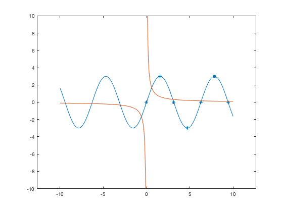
As you may see, this could get confusing to keep track of. Thus it may be easier to use the RGB triplets, and even name them ahead of time. This is discussed in the section below.

Using RGB triplets to change colors

One can specify colors using a vector that gives the RGB triple where in MATLAB, each of the three values are numbers from 0 to 1. Usually RGB colors have values from 0 to 255. You can use those numbers and divide the vector by 255 to use within MATLAB. Thus knowing the MATLAB RGB triples for the colors can be useful. From the table above, we can define the default colors to work with them or can put in the RGB triplet (as a vector) directly into the plot command. Both are shown in this example.

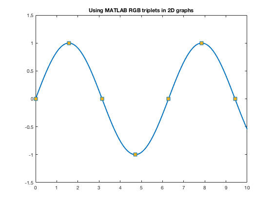
For other colors, you can look up their RGB code on many websites such as RGB Color Codes Chart or HTML Color Picker to see the RGB codes (or hex codes, etc.) For example, at these RGB Color websites, you will be given R=255, G=0, B=0 for red. So you can use 1/255[255,0,0] to get the color of red to use as a color in MATLAB.

The official color for Loyola Green is given as RGB:0-104-87, and Loyola Gray is given as RGB:200-200-200 (found on Loyola’s Logos/University Signature page. Here’s how one can use those colors in MATLAB.

Now one can use these colors to specify the color of markers, lines, edges, faces, etc.

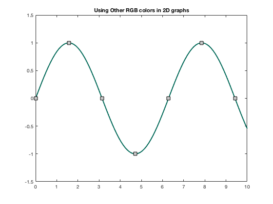
Changing colors in 3D Graphs

If using mesh(x,y,z), to change the look of it you can change to a different colormap as discussed in https://www.mathworks.com/help/matlab/ref/colormap.html. This was done above when showing the previous default colormap. Here are some more.

Warning! Once you change the colormap, it will keep that colormap for all subsequent 3D plots within the same figure or MATLAB session until you use close, or open a new figure window.

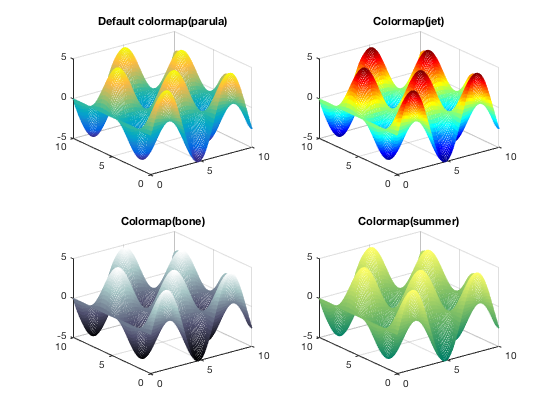
For mesh and surf, you can change ‘EdgeColor’ and/or ‘FaceColor’ to be uniform, rather than using colormaps.

Источник

Пакет MatLab позволяет
отображать графики с разным цветом и типом линий, показывать или скрывать сетку
на графике, выполнять подпись осей и графика в целом, создавать легенду и
многое другое. В данном параграфе рассмотрим наиболее важные функции,
позволяющие делать такие оформления на примере двумерных графиков.

Функция plot() позволяет
менять цвет и тип отображаемой линии. Для этого, используются дополнительные
параметры, которые записываются следующим образом:

plot(<x>, <y>, <’цвет линии, тип линии, маркер точек’>);

Обратите
внимание, что третий параметр записывается в апострофах и имеет обозначения,
приведенные в таблицах 3.1-3.3. Маркеры, указанные ниже записываются подряд
друг за другом, например,

‘ko’ – на графике отображает черными кружками точки графика,


‘ko-‘ – рисует

график черной линией и проставляет точки в виде кружков.

Табл.
3.1. Обозначение цвета линии графика

Маркер	Цвет линии
c	голубой
m	фиолетовый
y	желтый
r	красный
g	зеленый
b	синий
w	белый
k	черный

Табл.
3.2. Обозначение типа линии графика

Маркер	Цвет линии
—	непрерывная
—	штриховая
:	пунктирная
-.	штрих-пунктирная

Табл.
3.3. Обозначение типа точек графика

Маркер	Цвет линии
.	точка
+	плюс
*	звездочка
o	кружок
x	крестик

Ниже показаны примеры записи функции plot() с разным
набором маркеров.

x = 0:0.1:2*pi;


y = sin(x);
 
subplot(2,2,1);

plot(x,y,'r-');
subplot(2,2,2);

plot(x,y,'r-',x,y,'ko');
subplot(2,2,3);

plot(y,'b--');
subplot(2,2,4);

plot(y,'b--+');

Результат работы фрагмента программы
приведен на рис. 3.7. Представленный пример показывает, каким образом можно
комбинировать маркеры для достижения требуемого результата. А на рис. 3.7
наглядно видно к каким визуальным эффектам приводят разные маркеры,
используемые в программе. Следует особо отметить, что в четвертой строчке
программы по сути отображаются два графика: первый рисуется красным цветом и
непрерывной линией, а второй черными кружками заданных точек графика. Остальные
варианты записи маркеров очевидны.

Рис. 3.7. Примеры отображения графиков с разными
типами маркеров

Из примеров рис. 3.7 видно, что масштаб
графиков по оси Ox несколько больше реальных значений. Дело в том, что
система MatLab автоматически
масштабирует систему координат для полного представления данных. Однако такая
автоматическая настройка не всегда может удовлетворять интересам пользователя.
Иногда требуется выделить отдельный фрагмент графика и только его показать
целиком. Для этого используется функция axis() языка MatLab, которая имеет
следующий синтаксис:

axis( [ xmin, xmax, ymin, ymax ] ),

где
название указанных параметров говорят сами за себя.

Воспользуемся данной функцией для
отображения графика функции синуса в пределах от 0 до :

x = 0:0.1:2*pi;


y = sin(x);
 
subplot(1,2,1); 
plot(x,y);
axis([0 2*pi -1 1]);
 
subplot(1,2,2); 
plot(x,y);
axis([0 pi 0 1]);

Из результата работы программы (рис.
3.8) видно, что несмотря на то, что функция синуса задана в диапазоне от 0 до , с помощью функции
axis() можно
отобразить как весь график, так и его фрагмент в пределах от 0 до .

Рис. 3.8. Пример работы функции axis()

В заключении данного параграфа
рассмотрим возможности создания подписей графиков, осей и отображения сетки на
графике. Для этого используются функции языка MatLab, перечисленные
в табл. 3.4.

Таблица 3.4. Функции оформления графиков

Название	Описание
grid [on, off]	Включает/выключает сетку на графике
title(‘заголовок графика’)	Создает надпись заголовка графика
xlabel(‘подпись оси Ox’)	Создает подпись оси Ox
ylabel(‘подпись оси Oy’)	Создает подпись оси Oy
text(x,y,’текст’)	Создает текстовую надпись в координатах (x,y).

Рассмотрим работу данных функций в
следующем примере:

x = 0:0.1:2*pi;


y = sin(x);
 
plot(x,y);
axis([0 2*pi -1 1]);
grid on;
title('The graphic of sin(x)

function');
xlabel('The coordinate of

Ox');
ylabel('The coordinate of

Oy');
text(3.05,0.16,'leftarrow

sin(x)');

Из результата работы данной программы,
представленного на рис. 3.9, видно каким образом работают функции создания
подписей на графике, а также отображение сетки графика.

Таким образом, используя описанный набор
функций и параметров, можно достичь желаемого способа оформления графиков в
системе MatLab.

Рис. 3.9. Пример работы функций
оформления графика

Оглавление

Введение
Глава 1. Структура программы. Основные математические операции и типы данных
1.1. Структура программы пакета MatLab
1.2. Простые переменные и основные типы данных в MatLab
1.3. Арифметические операции с простыми переменными
1.4. Основные математические функции MatLab
1.5. Векторы и матрицы в MatLab
1.6. Операции над матрицами и векторами
1.7. Структуры в MatLab
1.8. Ячейки в MatLab
Глава 2. Условные операторы и циклы в MatLab
2.1. Условный оператор if
2.2. Условный оператор switch
2.3. Оператор цикла while
2.4. Оператор цикла for
Глава 3. Работа с графиками в MatLab
3.1. Функция plot
3.2. Оформление графиков
3.3. Отображение трехмерных графиков
3.4. Отображение растровых изображений
Глава 4. Программирование функций в MatLab
4.1. Порядок определения и вызова функций
4.2. Область видимости переменных
Глава 5. Работа с файлами в MatLab
5.1. Функции save и load
5.2. Функции fwrite и fread
5.3. Функции fscanf и fprintf
5.4. Функции imread и imwrite

Источник

Время прочтения
3 мин

Просмотры 56K

Недавно, в очередной раз проверяя домашние работы своих студентов, я загорелся желанием автоматизировать этот процесс. Задание состояло в составлении рабочей таблицы девиации магнитного компаса и построения кривой девиации.

Входными данными служили показания магнитного компаса (МК), синхронно наблюдаемые показания гирокомпаса (ГК), поправка ГК и значение магнитного склонения для района, в котором проходили измерения.

Все данные были занесены в таблицу и разделены из 10 столбцов с входными данными и 25 строк – значений входных данных для каждого из вариантов. Для удобства считывания данных в MATLAB они были записаны в виде текстового файла и импортировались в рабочее пространство с помощью функции importdata.

По методике расчетов необходимо было обработать данные с помощью нескольких эмпирических формул для заполнения рабочей таблицы девиации МК. Однако, основным и наиболее наглядным результатом работы является построение кривой девиации МК.

Для построения графика была выбрана функция plot, имеющая большое количество параметров настройки, которые позволяют получить результат в нужном виде. Был составлен код:

%Построение графика Рабочей кривой девиации
X=[0:10:360];
Y=SC;
plot(X,Y,'bo-');
grid on;
title('Рабочая кривая девиации');
xlabel('Компасный курс, circ');
ylabel('Девиация, circ');
axis auto
xlim([0,360])
set(gca, 'XTick',0:45:360)

И получен следующий график:

Разберем код построчно, рассмотрим какие параметры можно указывать для настройки отображения графиков.

X=[0:10:360];
Y=SC;

Здесь задаются входные данные для построения графика. Количество значений по оси абсцисс и по оси ординат должно совпадать. По эти данные являются векторами с 36 значениями.

plot(X,Y,'bo-');

Собственно, функция построения графика, в которую передаются данные и параметры. Помимо очевидных входных данных параметром функции является тип отображаемой линии, закодированный трехсимвольным сочетанием. В данном случае “b” – blue, цвет линии; “o” – вид маркера, которым обозначаются точки графика и “-” – тип линии, в данном случае – сплошная.

Ниже привожу список параметров для настройки отображаемой линии.

Маркер Цвет линии
c голубой
m фиолетовый
y желтый
r красный
g зеленый
b синий
w белый
k черный

Маркер Тип линии
— непрерывная
— — штриховая
: пунктирная
-. штрих-пунктирная

Маркер Тип маркера
. точка
+ знак «плюс»
* знак «звездочка»
о круг
х знак «крест»

grid on;

Команда, которой включается сетка на графике.

title('Рабочая кривая девиации');
xlabel('Компасный курс, circ');
ylabel('Девиация, circ');

Подписи для графика и соответствующих осей. Здесь “circ” кодировка символа градуса.

axis auto

Команда управления осями. В данном случае выставлен параметр “auto” – автоматическая расстановка осей. Здесь-то меня и не устроила работа MATLAB, т.к. автоматически оси не пристыковывались к крайним значениям графика, а «добавляли» лишнее пространство по оси “X”.

С помощью команды “help axis” я нашел еще несколько вариантов параметра для осей, в частности попробовал параметр “tight”, который должен был пристыковывать границы графика к крайним значениям кривой. Однако результат и этого параметра меня не удовлетворил т.к. результат выглядел следующим образом:

График выглядит «зажатым», к тому же «теряются» части кривой находящиеся между максимальными значениями.

Для получения наглядного результата пришлось настроить ось “X” отдельно с помощью следующих команд:

axis auto
xlim([0,360])

Последняя функция задает граничные значения отдельно для оси “X”, что позволило мне ограничить график максимальными значениями по данной оси.

И последняя команда:

set(gca, 'XTick',0:45:360)

Позволила настроить подписи и шаг для оси “X”. Функция “set” является достаточно общей, ее работа зависит от передаваемых параметров. В данном случае “gca” – означает, что параметры будут устанавливаться для сетки графика, “ XTick ” – означает, что будет управляться подпись оси “X”, а параметр “0:45:360” – задает минимальное значение, шаг и максимальное значение.

В результате получился достаточно наглядный график кривой девиации, по сравнению формы которого с формой графика полученного студентом можно было быстро оценить правильность выполнения работы. Так же, благодаря загрузке данных из файла по всем вариантам, с дальнейшим выбором последнего, изменять приходилось только номер варианта, чтобы получить результат.

Надеюсь, что эта статья будет полезной не только для начинающих MATLAB, но и для опытных пользователей.

В окончании хотел бы отметить полезность команды “help” – она не только позволяет получить необходимую информацию по функции или команде из командной строки, но и сделать это значительно быстрее, чем через поиск в справке MATLAB.

Источник

Types of Color Values

Specify Color of a Bar Chart

Specify Marker Colors in a Scatter Plot

Specify Colors in a Series of Plots

See Also

Functions

Properties

Related Topics

Syntax

Description

Vector and Matrix Data

Table Data

Additional Options

Examples

Create Line Plot

Plot Multiple Lines

Create Line Plot From Matrix

Specify Line Style

Specify Line Style, Color, and Marker

Display Markers at Specific Data Points

Specify Line Width, Marker Size, and Marker Color

Add Title and Axis Labels

Plot Durations and Specify Tick Format

Plot Coordinates from a Table

Plot Multiple Table Variables on One Axis

Specify Axes for Line Plot

Modify Lines After Creation

Plot Circle

Input Arguments

X — x-coordinates scalar | vector | matrix

Y — y-coordinates scalar | vector | matrix

LineSpec — Line style, marker, and color string | character vector

tbl — Source table table | timetable

xvar — Table variables containing x-coordinates string array | character vector | cell array | pattern | numeric scalar or vector | logical vector | vartype()

yvar — Table variables containing y-coordinates string array | character vector | cell array | pattern | numeric scalar or vector | logical vector | vartype()

ax — Target axes Axes object | PolarAxes object | GeographicAxes object

Name-Value Arguments

Color — Line color [0 0.4470 0.7410] (default) | RGB triplet | hexadecimal color code | "r" | "g" | "b" | …

DatetimeTickFormat — Format for datetime tick labels character vector | string

DurationTickFormat — Format for duration tick labels character vector | string

Tips

Extended Capabilities

Tall Arrays Calculate with arrays that have more rows than fit in memory.

GPU Arrays Accelerate code by running on a graphics processing unit (GPU) using Parallel Computing Toolbox™.

Distributed Arrays Partition large arrays across the combined memory of your cluster using Parallel Computing Toolbox™.

Version History

R2022b: Plots created with tables preserve special characters in axis and legend labels

R2022a: Pass tables directly to plot

plot

Синтаксис

Описание

Примеры

Построение графика

Построение нескольких графиков

Построение графика из матрицы

Определение стиля линии

Определение стиля линии, цвета и маркера

Отображение маркеров в определенных точках данных

Определение ширины линии, размера маркера и цвета маркера

Добавление заголовка и подписей по осям

Графическое изображение длительности и определение формата метки деления

Задание осей для графика

Изменение линни после ее создания

Рисование окружности

Входные параметры

X — x — координаты скаляр | вектор | матрица

Y — y — координаты скаляр | вектор | матрица

LineSpec — Стиль линии, маркер и цвет вектор символов | строка

ax — Целевые оси Axes возразите | PolarAxes возразите | GeographicAxes объект

Аргументы name-value

Color ‘LineColor’ [0 0.4470 0.7410] (значение по умолчанию) | триплет RGB | шестнадцатеричный цветовой код | 'r' | 'g' | 'b' | …

DatetimeTickFormat — Формат для datetime метки в виде галочки вектор символов | строка

DurationTickFormat — Формат для duration метки в виде галочки вектор символов | строка

Советы

Расширенные возможности

«Высокие» массивы Осуществление вычислений с массивами, которые содержат больше строк, чем помещается в памяти.

Массивы графического процессора Ускорьте код путем работы графического процессора (GPU) с помощью Parallel Computing Toolbox™.

Распределенные массивы Большие массивы раздела через объединенную память о вашем кластере с помощью Parallel Computing Toolbox™.

GraphPlot Properties

Nodes

`X` — x-coordinates
scalar | vector | matrix

`Y` — y-coordinates
scalar | vector | matrix

`LineSpec` — Line style, marker, and color
string | character vector

`tbl` — Source table
table | timetable

`xvar` — Table variables containing x-coordinates
string array | character vector | cell array | pattern | numeric scalar or vector | logical vector | `vartype()`

`yvar` — Table variables containing y-coordinates
string array | character vector | cell array | pattern | numeric scalar or vector | logical vector | `vartype()`

`ax` — Target axes
`Axes` object | `PolarAxes` object | `GeographicAxes` object

`Color` — Line color
`[0 0.4470 0.7410]` (default) | RGB triplet | hexadecimal color code | `"r"` | `"g"` | `"b"` | …

`DatetimeTickFormat` — Format for `datetime` tick labels
character vector | string

`DurationTickFormat` — Format for `duration` tick labels
character vector | string

Tall Arrays
Calculate with arrays that have more rows than fit in memory.

GPU Arrays
Accelerate code by running on a graphics processing unit (GPU) using Parallel Computing Toolbox™.

Distributed Arrays
Partition large arrays across the combined memory of your cluster using Parallel Computing Toolbox™.

R2022a: Pass tables directly to `plot`

`X` — x — координаты
скаляр | вектор | матрица

`Y` — y — координаты
скаляр | вектор | матрица

`LineSpec` — Стиль линии, маркер и цвет
вектор символов | строка

`ax` — Целевые оси
`Axes` возразите | `PolarAxes` возразите | `GeographicAxes` объект

`Color` ‘LineColor’
[0 0.4470 0.7410] (значение по умолчанию) | триплет RGB | шестнадцатеричный цветовой код | `'r'` | `'g'` | `'b'` | …

`DatetimeTickFormat` — Формат для `datetime` метки в виде галочки
вектор символов | строка

`DurationTickFormat` — Формат для `duration` метки в виде галочки
вектор символов | строка

«Высокие» массивы
Осуществление вычислений с массивами, которые содержат больше строк, чем помещается в памяти.

Массивы графического процессора
Ускорьте код путем работы графического процессора (GPU) с помощью Parallel Computing Toolbox™.

Распределенные массивы
Большие массивы раздела через объединенную память о вашем кластере с помощью Parallel Computing Toolbox™.

`NodeColor` — Node color
`[0 0.4470 0.7410]` (default) | RGB triplet | hexadecimal color code | color name | matrix | `'flat'` | `'none'`

`Marker` — Node marker symbol
`'o'` (default) | character vector | cell array | string vector

`MarkerSize` — Node marker size
positive value | vector

`NodeCData` — Color data of node markers
vector

`EdgeColor` — Edge color
`[0 0.4470 0.7410]` (default) | RGB triplet | hexadecimal color code | color name | matrix | `'flat'` | `'none'`

`LineStyle` — Line style
`'-'` (default) | `'--'` | `':'` | `'-.'` | `'none'` | cell array | string vector

`LineWidth` — Edge line width
`0.5` (default) | positive value | vector

`EdgeAlpha` — Transparency of graph edges
`0.5` (default) | scalar value between `0` and `1` inclusive

`EdgeCData` — Color data of edge lines
vector

`ArrowSize` — Arrow size
positive value | vector of positive values

`ArrowPosition` — Position of arrow along edge
`0.5` (default) | scalar | vector

`ShowArrows` — Toggle display of arrows on directed edges
on/off logical value

`XData` — x-coordinate of nodes
vector

`YData` — y-coordinate of nodes
vector

`ZData` — z-coordinate of nodes
vector

`NodeLabel` — Node labels
node IDs (default) | vector | cell array of character vectors

`NodeLabelMode` — Selection mode for node labels
`'auto'` (default) | `'manual'`

`NodeLabelColor` — Color of node labels
`[0 0 0]` (default) | RGB triplet | hexadecimal color code | color name | matrix

`EdgeLabel` — Edge labels
`{}` (default) | vector | cell array of character vectors

`EdgeLabelMode` — Selection mode for edge labels
`'manual'` (default) | `'auto'`

`EdgeLabelColor` — Color of edge labels
`[0 0 0]` (default) | RGB triplet | hexadecimal color code | color name | matrix

`Interpreter` — Interpretation of text characters
`'tex'` (default) | `'latex'` | `'none'`

`NodeFontName` — Font name for node labels
`'Helvetica'` (default) | supported font name | `'FixedWidth'`

`NodeFontSize` — Font size for node labels
`8` (default) | positive number | vector of positive numbers

`NodeFontWeight` — Thickness of text in node labels
`'normal'` (default) | `'bold'` | vector | cell array

`NodeFontAngle` — Character slant of text in node labels
`'normal'` (default) | `'italic'` | vector | cell array

`EdgeFontName` — Font name for edge labels
`'Helvetica'` (default) | supported font name | `'FixedWidth'`

`EdgeFontSize` — Font size for edge labels
`8` (default) | positive number | vector of positive numbers

`EdgeFontWeight` — Thickness of text in edge labels
`'normal'` (default) | `'bold'` | vector | cell array

`EdgeFontAngle` — Character slant of text in edge labels
`'normal'` (default) | `'italic'` | vector | cell array

`DisplayName` — Text used by legend
`''` (default) | character vector

`Annotation` — Legend icon display style
`Annotation` object

`DataTipTemplate` — Data tip content
`DataTipTemplate` object

`ButtonDownFcn` — Mouse-click callback
`''` (default) | function handle | cell array | character vector

`CreateFcn` — Creation callback
`''` (default) | function handle | cell array | character vector

`DeleteFcn` — Deletion callback
`''` (default) | function handle | cell array | character vector

`BusyAction` — Callback queuing
`'queue'` (default) | `'cancel'`

`PickableParts` — Ability to capture mouse clicks
`'visible'` (default) | `'none'`

`Parent` — Parent of GraphPlot
axes object | group object | transform object

`HandleVisibility` — Visibility of object handle
`'on'` (default) | `'off'` | `'callback'`

`Type` — Type of graphics object
`'graphplot'`

`Tag` — Tag to associate with GraphPlot
`''` (default) | character vector

`UserData` — Data to associate with GraphPlot
`[]` (default) | scalar, vector, or matrix | cell array | character array | table | structure

R2020a: `UIContextMenu` property is not recommended