Description
You can use zoom mode to explore data by interactively changing the limits of
axes. Enable or disable zoom mode, and set other basic options, by using the
zoom function. To further control zoom mode behavior, return and use a
zoom object.
Most charts support zoom mode, including line, bar, histogram, and surface charts. Charts
that support zoom mode typically display the zoom in ![]() and zoom out
and zoom out ![]() icons in the axes toolbar.
icons in the axes toolbar.
You can also interactively explore data using built-in axes interactions that are enabled
by default. For example, you can zoom in and out of the view of the axes by scrolling or
pinching. Built-in interactions do not require you to enable an interaction mode and respond
faster than interaction modes. However, you can enable zoom mode to customize the zooming
behavior. For more information about built-in interactions, see Control Chart Interactivity.
Creation
Syntax
Description
example
zoom sets the zoom mode for alloption
axes in the current figure. For example, zoom on enables zoom mode,
zoom xon enables zoom mode for the x-dimension
only, and zoom off disables zoom mode.
When zoom mode is enabled, zoom the view of the axes using the cursor, the scroll
wheel, or the keyboard.
-
Cursor — To zoom in, position your cursor where you want the center of
the axes to be and click. To zoom out, hold Shift and click. To
zoom into a rectangular region, click and drag. To return an axes object to its
baseline zoom level, double-click within the axes. -
Scroll wheel — To zoom in, scroll up. To zoom out, scroll down.
-
Keyboard — To zoom in, press the up arrow (↑) key. To
zoom

                      out
, press the down arrow (↓) key.
Some built-in interactions remain enabled by default, regardless of the current
interaction mode. To disable built-in zoom interactions that are independent of the zoom
mode, use the disableDefaultInteractivity function.
zoom toggles the zoom mode. If zoom mode is disabled, then
calling zoom restores the most recently used zoom option of
on, xon, or yon.
zoom( zooms the current axes by thefactor)
specified zoom factor without affecting the zoom mode. Zoom in by specifying
factor as a value greater than 1, for example,
zoom(3). Zoom out by specifying factor as a
value between 0 and 1, for example, zoom(0.5).
zoom( sets the zoomfig,___)
mode for all axes in the specified figure for any of the previous syntaxes. Specify the
additional argument as a zoom mode option or a zoom factor. For example, use
zoom(fig,'on') to enable zoom mode for the figure
fig, or use zoom(fig,2) to zoom all axes in the
figure fig by a factor of 2.
example
z = zoom creates a zoom object for the current
figure. This syntax is useful for customizing the zoom mode, motion, and
direction.
example
z = zoom( creates afig)
zoom object for the specified figure.
Input Arguments
expand all
option — Zoom mode option
'on' | 'off' | 'reset' | 'out' | 'xon' | 'yon' | 'toggle'
Zoom mode option, specified as one of these values:
-
'on'— Enable zoom mode. -
'off'— Disable zoom mode. Some built-in
interactions remain enabled by default, regardless of the current interaction
mode. To disable built-in zoom interactions that are independent of the zoom
mode, use thedisableDefaultInteractivityfunction. -
'reset'— Set the current zoom level as the
baseline zoom level. Once you set the baseline zoom level, callingzoom, double-clicking in the axes, or clicking the Restore View
out
 icon from the axes toolbar returns axes to this
zoom level. -
'out'— Return the current axes to its baseline
zoom level. -
'xon'— Enable zoom mode for the
x-dimension only. -
'yon'— Enable zoom mode for the
y-dimension only. -
'toggle'— Toggle the zoom mode. If zoom mode is
disabled, then'toggle'restores the most recently used zoom
option of'on','xon', or
'yon'. Using this option is the same as calling
zoomwithout any arguments.
factor — Zoom factor
positive number
Zoom factor, specified as a positive number. Zoom in by specifying
factor as a number greater than 1. Zoom out by specifying
factor as a number between 0 and 1. In this case, the axes zoom
out by 1/factor.
fig — Target figure
Figure object
Target figure, specified as a Figure object.
Properties
expand all
Motion — Dimension
'both' (default) | 'horizontal' | 'vertical'
Dimension to allow zooming in and out, specified as one of these values:
-
'both'— Allow zooming in the
x-dimension and the y-dimension. -
'horizontal'— Allow zooming in the
x-dimension only. -
'vertical'— Allow zooming in the
y-dimension only.
This property affects only axes in a 2-D view, such as when you call
view([0 90]). To control the zoom dimension in 3-D views, use a
ZoomInteraction object.
Direction — Direction
'in' (default) | 'out'
Direction of zooming, specified as one of these values:
-
'in'— Click to zoom in. -
'out'— Click to zoom out.
When zoom mode is enabled, you can use the scroll wheel to zoom in or out,
regardless of the value of Direction.
RightClickAction — Action to perform on right-click
'PostContextMenu' (default) | 'InverseZoom'
Action to perform on right-click, specified as one of these values:
-
'PostContextMenu'— Display a context menu. -
'InverseZoom'— Zoom out on right-click.
Setting the RightClickAction property sets the
default for future zoom objects. The value of
RightClickAction persists between MATLAB® sessions.
— Context menu
empty GraphicsPlaceholder array (default) | ContextMenu object
Context menu, specified as a ContextMenu object. Use this property
to display a context menu when you right-click in axes where zoom mode is enabled.
Create the context menu using the uicontextmenu function.
This property has no effect if the RightClickAction property
has a value of 'InverseZoom'.
ButtonDownFilter — Zoom suppression callback
[ ] (default) | function handle | cell array | character vector
Zoom suppression callback, specified as one of these values:
-
Function handle
-
Cell array containing a function handle and additional arguments
-
Character vector containing a valid MATLAB command or function, which is evaluated in the base workspace (not
recommended)
Use this property to suppress zooming under conditions that you define. A numeric or
logical output of 1 (true) suppresses zooming, and a numeric or
logical output of 0 (false) allows zooming. If you specify this
property using a function handle, then MATLAB passes two arguments to the callback function:
-
axes— The axes object in which you are
zooming. -
eventData— Empty argument. Replace it with the tilde
character (~) in the function definition to indicate that this
argument is not used.
If you specify this property using a function handle, then you must assign the
function output to a variable.
For more information about callbacks, see Create Callbacks for Graphics Objects.
ActionPreCallback — Function to execute before zooming
[ ] (default) | function handle | cell array | character vector
Function to execute before zooming, specified as one of these values:
-
Function handle
-
Cell array containing a function handle and additional arguments
-
Character vector containing a valid MATLAB command or function, which is evaluated in the base workspace (not
recommended)
Use this property to execute code as you start zooming in or out. If you specify
this property using a function handle, then MATLAB passes two arguments to the callback function:
-
figure—Figureobject in which you
are zooming. -
axesStruct— Structure that contains one field,
Axes, the axes object in which you are zooming. If you do not
use this argument in your callback function, then replace it with the tilde
character (~).
For more information about callbacks, see Create Callbacks for Graphics Objects.
ActionPostCallback — Function to execute after zooming
[ ] (default) | function handle | cell array | character vector
Function to execute after zooming, specified as one of these values:
-
Function handle
-
Cell array containing a function handle and additional arguments
-
Character vector containing a valid MATLAB command or function, which is evaluated in the base workspace (not
recommended)
Use this property to execute code after you finish zooming. If you specify this
property using a function handle, then MATLAB passes two arguments to the callback function:
-
figure—Figureobject in which you
are zooming. -
axesStruct— Structure that contains one field,
Axes, the axes object in which you are zooming. If you do not
use this argument in your callback function, then replace it with the tilde
character (~).
For more information about callbacks, see Create Callbacks for Graphics Objects.
Enable — Zoom mode state
'off' (default) | 'on'
Zoom mode state, specified as 'off' or
'on'.
FigureHandle — Figure object
Figure object
This property is read-only.
Figure object that you specified when creating the
zoom object. If you did not specify a figure, then
FigureHandle is the figure that was current when you created the
zoom object.
UseLegacyExplorationModes — Legacy mode
'off' (default) | 'on' | on/off logical value
Legacy mode, specified as 'on' or 'off', or as
numeric or logical 1 (true) or
0 (false). A value of 'on' is
equivalent to true, and 'off' is equivalent to
false. Thus, you can use the value of this property as a logical
value. The value is stored as an on/off logical value of type OnOffSwitchState.
This property applies only to zoom objects for figures created
using the uifigure function or in MATLAB
Online™. Setting this property to 'on' changes the behavior of
interaction modes in UI figures so they match the behavior of modes in traditional
figures. For more information, see enableLegacyExplorationModes.
Once this property is set to 'on', it cannot be changed back to
'off'.
Object Functions
Use zoom object functions to customize the zooming behavior of axes objects within a
figure. For all of these functions, the axes and zoom objects must be associated with the same
figure.
|
|
The Calling Enabling zoom mode for axes using |
|
|
The Calling Returning the zoom |
|
|
The Calling Setting the zoom dimension for |
|
|
The Calling Returning the zoom dimension of axes using |
|
|
The Calling For more information about the camera view angle, see Camera Graphics Terminology. |
|
|
The Calling |
|
|
This function is not recommended. Use Calling The axes |
|
|
This function is not recommended. Use Calling The axes zoom dimension that is returned using |
Examples
collapse all
Set Baseline Zoom Level
Plot a surface and enable zoom mode.
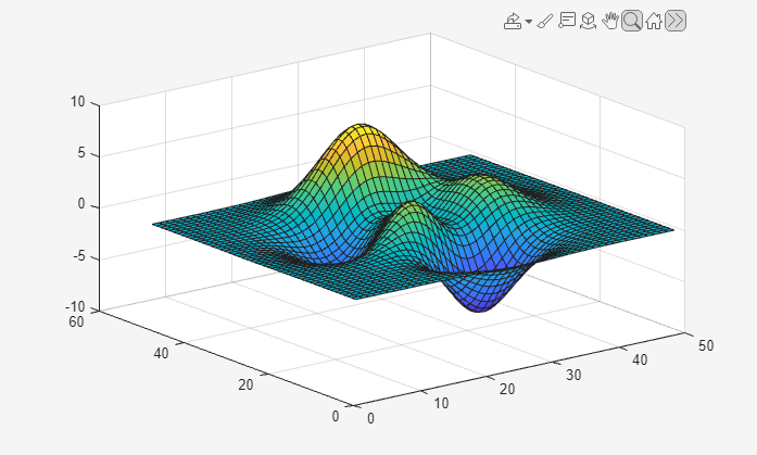
Zoom into the tallest peak by clicking on it. Then, set the baseline zoom level.
Future calls to zoom out, double-clicking in the axes, or clicking
selecting the Restore View ![]() icon from the axes toolbar return axes to this baseline
icon from the axes toolbar return axes to this baseline
zoom level.
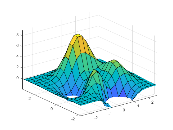
Zoom into the highest peak a second time by clicking on it. Then, return to the
baseline zoom level you set by zooming out.
Constrain Zoom in Tiled Chart Layout
Create four axes in a tiled chart layout, and assign each a different zoom behavior.
Then, interactively zoom the axes.
tiledlayout(2,2)
ax1 = nexttile;
plot(1:10);
z = zoom;

ax2 = nexttile;
plot(rand(3));
setAllowAxesZoom(z,ax2,false);

ax3 = nexttile;
surf(peaks);
setAxesZoomConstraint(z,ax3,'xy');

ax4 = nexttile;
contour(peaks);
setAxesZoomMotion(z,ax4,'horizontal');
Create Mode Context Menu
Plot a surface and create a context menu using the uicontextmenu function.
surf(peaks)
cm = uicontextmenu;
Then, add an item to the menu. Specify a label and a callback that closes the
figure.
m = uimenu(cm);
m.Label = 'Close figure';
f = gcf;
m.Callback = @(src,event)close(f);
Create a zoom object. Add the context menu to the zoom object by setting its
ContextMenu property. Then, enable zoom mode.
z = zoom(f);
z.ContextMenu = cm;
z.Enable = 'on';
Close the figure by right-clicking and selecting .
More About
expand all
Changing Callback Functions
You can create a zoom object and use it to customize the behavior
of different axes. You can also change its callback functions on the fly.
Note
Do not change figure callbacks within an interactive
mode. While a mode is active (such as when zoom mode is enabled), you will
receive a warning if you attempt to change any of the figure’s keyboard callbacks or
window callbacks, and the operation will not succeed. The one exception to this rule is
the figure WindowButtonMotionFcn callback, which can be changed from
within a mode. Therefore, if you are creating a UI that updates a figure’s callbacks, the
UI should keep track of and check which interactive mode is active, if any, before
attempting to change a callback.
When you assign different zoom behaviors to different axes in a figure by using mode
objects and then link them using the linkaxes function, the behavior of
the axes you manipulate with the mouse carries over to the linked axes, regardless of the
behavior you previously set for the other axes.
Alternative Functionality
Axes Toolbar
For some charts, enable zoom mode by clicking the zoom in ![]() or zoom out
or zoom out ![]() icons in the axes toolbar.
icons in the axes toolbar.
Version History
Introduced before R2006a
expand all
R2020a: UIContextMenu property is not recommended
Starting in R2020a, using the UIContextMenu property to assign a
context menu to a graphics object or UI component is not recommended. Use the
ContextMenu property instead. The property values are the
same.
There are no plans to remove support for the UIContextMenu property
at this time. However, the UIContextMenu property no longer appears in
the list returned by calling the get function on a graphics object or UI
component.
R2018b: Explore data with zooming enabled by default
Interactively explore your data using built-in axes interactions that are enabled by
default. For example, you can use the scroll wheel to zoom into your data without enabling
zoom mode. For more information, see Control Chart Interactivity.
Previously, no axes interactions were enabled by default.

Добавил:
Upload
Опубликованный материал нарушает ваши авторские права? Сообщите нам.
Вуз:
Предмет:
Файл:
Скачиваний:
320
Добавлен:
02.04.2015
Размер:
1.62 Mб
Скачать

Основы графики в MATALB
Одной из особенностей MATLAB являются простые и мощные возможности по построению графиков. В самом простом случае для построения графика достаточно использования функцию plot. В наиболее простом случае функция plot принимает 2 аргумента: два вектора одинаковой длины, задающие точки для построения графика. Первый аргумент это координаты точек по оси абсцисс, а второй соответствующие координаты по оси ординат. Приведем пример использования этой функции для построения графика
sin( x) :
%пример использования функции plot
%координаты точек для построения графика по оси абсцисс x = -2*pi : 0.5 : 2*pi;
%координаты точек для построения графика по оси ординат y = sin(x);
%строим график по точкам, координаты которых содержатся в x, y plot(x, y);
Врезультате выполнения данного скрипта появится следующие окно с графиком:
Данный пример построения графика является наиболее, простым и не содержит не какого-либо описания, подписей, обозначений, поэтому далее рассмотрим способы оформления графиков в MATLAB.
Оформление графиков
В данном пункте рассмотрим основные функции и команды для оформления графиков.
62

Для создания заголовка текущего графика используется функция title, принимающая заголовок в виде строки и выводящая его над графиком, например:
>> title(‘Exaple graphic’);
Для того чтобы подписать ось абсцисс и ось ординат используются функции xlabel и ylabel соответственно, которые принимаю название осей, например:
>>xlabel(‘x’);
>>ylabel(‘y’);
Теперь рассмотрим функцию legend, выводящую легенду графика. Данную функцию удобно использовать, когда с одних и тех же осей строится несколько графиков (такой пример будет рассмотрен в следующих пунктах). Данная функция принимает названия графиков через запятую, которые содержатся на текущих осях. Например:
legend(‘y=sin(x)’);
Далее рассмотрим как задать масштаб графика. По умолчанию MATLAB автоматически выбирает масштаб графика, что довольно удобно, однако в некоторых случаях масштаб графика по умолчанию нас не всегда будет устраивать, и для задания его вручную используются функции xlim и ylim, принимающие массив из двух элементов, указывающие минимальные и максимальные значения для соответствующей оси, например:
xlim([-100 100]);
В данном случае ось абсцисс будет содержать отображать только значения от -100 до
100.
И последнее что необходимо отметить из основ оформления графиков это включение сетки, выполняющееся командой gird on, которая добавит сетку на текущий график:
>> grid on
Теперь продемонстрируем все представленные возможности по оформлению графика, на примере следующего скрипта:
%пример использования функции plot и функций для оформления графиков
%координаты точек для построения графика по оси абсцисс
x = -20*pi : pi/32 : 20*pi;
%координаты точек для построения графика по оси ординат y = sin(x) .* x;
%строим график по точкам, координаты которых содержатся в x, y plot(x, y);
63

%заголовок графика title(‘Example graphic’);
%подпишем оси xlabel(‘x’); ylabel(‘y’);
%легенда
legend(‘y = sin(x) * x (legend)’);
%масштаб графика
%по оси абсцисс xlim([-100 100]);
%по оси ординат ylim([-100 100]);
%включить сетку grid on
Врезультате выполнения данного скрипта появится следующее окно с графиком:
Вывод нескольких графиков в текущее окно
Для визуального сравнения нескольких графиков удобно строить несколько графиков в пределах одного окна и одной и той же системе координат. Для того чтобы добавить еще один график необходимо использовать команду hold all, после чего снова
64
воспользоваться функцией plot, например:
>>x = -10:0.1:10;
>>y1 = sin(x);
>>y2 = (x / 10) .^3;
>>plot(x, y1);
>>hold all
>>plot(x, y2);
Врезультате выполнения этих команд сформируется следующий график:
Отметим, что если не использовать команду hold all, то последний вызов функции plot затрет все предыдущие графики в текущем окне. Аналогичный результат можно получить и без использования функции hold, указа в plot сразу все графики, которые необходимо построить:
>> plot(x, y1, x, y2);
Построенный в этом случае график не будет отличаться от предыдущего. Однако чтобы этот график был построен в новых осях нужно либо убрать действие функции hold: hold off, или закрыть данное окно, чтобы функция plot создала новое окно с настройками по умолчанию, однако чтобы не делать это вручную, удобно будет воспользоваться функцией close:
>> close
Вызов данной функции без параметров закроек все открытые окна графиков.
65

Теперь рассмотрим способы задания цветов графиков, стилей линий и стилей точек графиков. Наиболее простой и удобный способ это написать строку с описание линии, после указания координат в функции plot(x, y, описание_линиии ), например:
plot(x,y,’-.or’);
Опишем некоторые из них (полное описание можно найти в справке MATLAB): Тип линии
•‘-‘ – сплошная;
•‘—‘ – штриховая линия;
•‘:’ – пунктирная линия;
•‘-.’ – штрихпунктирная линия. Тип маркера:
•‘+’ – знак плюс;
•‘o’ – круг;
•‘*’ – звездочка;
•‘.’ – точка;
•‘x’ – крестик.
Цвет линии и маркеров:
•‘r’ – красный;
•‘g’ – зеленый;
•‘b’ – синий;
•‘k’ – черный.
Тип линии, маркера и цвет могут следовать в строке в любой последовательности, например:
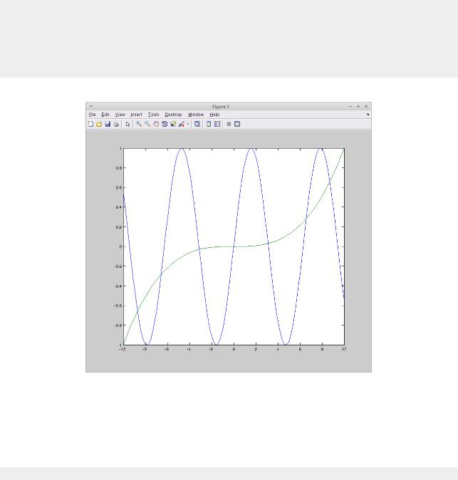
>>x = -1 : 0.1 : 1;
>>plot(x, sin(x), ‘—or’, x, sin(x+pi/2), ‘gx-.’, x, sin(x-pi/2), ‘*b:’);
legend(‘f1(x) = sin(x)’, ‘f2(x) = sin(x+pi/2)’, ‘f3(x) = sin(x-pi/2)’);
Созданный график будет выглядеть следующим образом:
66
Соседние файлы в папке Zadania_na_2_semestr
- #
- #
Иллюстрированный самоучитель по MatLab
Для изменения масштаба двумерных графиков используются команды класса zoom:
- zoom – переключает состояние режима интерактивного изменения масштаба для текущего графика;
- zoom (FACTOR) устанавливает масштаб в соответствии с коэффициентом FACTOR;
- zoom on – включает режим интерактивного изменения масштаба для текущего графика;
- zoom off – выключает режим интерактивного изменения масштаба для текущего графика;
- zoom out – обеспечивает полный просмотр, т. е. устанавливает стандартный масштаб графика;
- zoom xon или zoom yon – включает режим изменения масштаба только по оси х или по оси у;
- zoom reset – запоминает текущий масштаб в качестве масштаба по умолчанию для данного графика;
- zoom(FIG,OPTION) – применяется к графику, заданному дескриптором FIG, при этом OPTION может быть любым из перечисленных выше аргументов.
Команда zoom позволяет управлять масштабированием графика с помощью мыши. Для этого надо подвести курсор мыши к интересующей вас области рисунка. Если команда zoom включена (on), то нажатие левой кнопки увеличивает масштаб вдвое, а правой – уменьшает вдвое. При нажатой левой кнопке мыши можно выделить пунктирным черным прямоугольником нужный участок графика – при отпускании кнопки он появится в увеличенном виде и в том масштабе, который соответствует выделяющему прямоугольнику.
Рассмотрим работу команды zoom на следующем примере:
Рисунок 6.44 показывает график функции данного примера в режиме выделения его участка с помощью мыши.
После прекращения манипуляций левой кнопкой мыши график примет вид, показанный на рис. 6.44. Теперь в полный размер графического окна будет развернуто изображение, попавшее в выделяющий прямоугольник.
Рис. 6.43. Выделение части графика мышью при использовании команды zoom
Команда zoom, таким образом, выполняет функцию «лупы», позволяющей наблюдать в увеличенном виде отдельные фрагменты сложных графиков. Однако следует учитывать, что для наблюдения фрагментов графиков при высоком увеличении они должны быть заданы большим количеством точек. Иначе вид отдельных фрагментов и тем более особых точек (в нашем случае это точка при х вблизи нуля) будет существенно отличаться от истинного.
Как увеличить масштаб в matlab
Иллюстрированный самоучитель по MatLab
- zoom – переключает состояние режима интерактивного изменения масштаба для текущего графика;
- zoom (FACTOR) устанавливает масштаб в соответствии с коэффициентом FACTOR;
- zoom on – включает режим интерактивного изменения масштаба для текущего графика;
- zoom off – выключает режим интерактивного изменения масштаба для текущего графика;
- zoom out – обеспечивает полный просмотр, т. е. устанавливает стандартный масштаб графика;
- zoom xon или zoom yon – включает режим изменения масштаба только по оси х или по оси у;
- zoom reset – запоминает текущий масштаб в качестве масштаба по умолчанию для данного графика;
- zoom(FIG,OPTION) – применяется к графику, заданному дескриптором FIG, при этом OPTION может быть любым из перечисленных выше аргументов.
Как увеличить масштаб страницы в Matlab?
Масштабирование изображения в Matlab — интерполяция ближайшего соседа и билинейная интерполяция
Сначала рисуем шероховатую поверхность, а потом по-разному вставляем несколько точек, получившееся изображение будет следующим: 
Видно, что разные эффекты интерполяции различаются. Рисунок 1 очень грубый и имеет несколько точек рисования. Рисунок 2 — интерполяция ближайшего соседа, которая дает эффект, аналогичный «шагу». Изогнутая поверхность раньше выглядела более гладкой. Аналогично изображению, изображение, полученное с помощью интерполяции ближайшего соседа, эквивалентно увеличению пикселей, в то время как использование билинейной интерполяции и сферической интерполяции эквивалентно более плавному переходу между пикселями изображения.
Интерполяция ближайшего соседа, значение пиксельной точки, ближайшей к целевой точке, используется в качестве значения интерполяции 
Как показано на рисунке, изображение src MxN увеличивается до изображения dst PxQ. Нам нужно создать новый массив PXQ и случайным образом выбрать точку A (i, j) среди пикселей. , Предполагая, что мы используем изображение в градациях серого, каким должно быть значение в градациях серого в точке A?
Сначала мы сопоставляем координаты точки P с исходным изображением (я не знаю, не подходит ли отображение 😂), предполагая, что это точка B, тогда мы можем вычислить B по аналогии с аналогичными свойствами аналогичных треугольников. Координаты точки (x, y): (x, y) = (M/P*i, N/Q*j)
Поскольку индекс массива может быть только целым числом, x и y необходимо преобразовать в целые числа. При использовании интерполяции ближайшего соседа мы можем округлить в большую сторону:
Исходное изображение представляет собой цветное изображение размером 256×256: 
После использования интерполяции ближайшего соседа оно становится цветным изображением 768×768 (рекомендуется щелкнуть, чтобы увеличить и наблюдать): 
При билинейной интерполяции учитывается не только ближайший пиксель, но и взвешенное значение четырех окружающих пикселей. 
Как показано на рисунке, предположим, что все ABCD — это смежные пиксели, а (x, y) попадают в середину.
Влияние расстояния учитывается при интерполяции: чем дальше от пикселя, тем меньше вес, например точка A на рисунке, учитывая, что ABCD представляет собой квадрат со стороной 1, вы можете (1-dx) (1-dy) представляет собой вес серого значения точки A (для подробного доказательства, пожалуйста, обратитесь к блогу большого парня), где dx и dy представляют собой расстояние в направлениях x и y соответственно
Предполагая, что уровни серого в ABCD равны a, b, c и d соответственно, мы можем получить уровень серого в (x, y) как:
i n t e n s i t y = ( 1 − d x ) ( 1 − d y ) a + ( 1 − d x ) d y b + d x ( 1 − d y ) c + d x d y d ) intensity = (1-dx)(1-dy)a + (1-dx)dy b + dx(1-dy) c + dxdy d) i n t e n s i t y = ( 1 − d x ) ( 1 − d y ) a + ( 1 − d x ) d y b + d x ( 1 − d y ) c + d x d y d )
В Matlab координаты ABCD могут быть получены с помощью смелой функции округления,Обратите внимание, что в Matlab массив изображений начинается с 1, он должен быть округлен, а массив находится за пределами
В результате получится изображение 768×768 (рекомендуется щелкнуть, чтобы увеличить и посмотреть): 
Как увеличить / уменьшить масштаб в редакторе Matlab?
Мне интересно, есть ли способ увеличить / уменьшить масштаб или изменить размер шрифта или каким-либо образом сделать текст в коде в редакторе Matlab больше / меньше!
3 ответа
Вы переходите к Home->Preferences->MATLAB->Fonts и можете изменить размер текста. Если вы поиграете с окружающими предпочтениями, вы также сможете персонализировать больше вещей.
В зависимости от вашей версии MATLAB откройте окно «Preferences». По крайней мере, в более новых версиях это обычно находится в верхней части главного окна, на панели с надписью «Environment».
В открывшемся окне перейдите на вкладку «Шрифты». Вверху правой части окна вы найдете раскрывающееся меню, содержащее размер шрифта. Это влияет на размер шрифта в командном окне, редакторе и истории команд. Вы также можете изменить шрифт здесь.
Если кто-то еще задает эти вопросы в сообщении поисковой системы 2017 *: следующий код, по-видимому, увеличивает масштаб всего редактора MATLAB в 1,5 раза, но требует перезапуска MATLAB:
GraphPlot Properties
Graph plot appearance and behavior
GraphPlot properties control the appearance and behavior of
plotted graphs. By changing property values, you can modify aspects of the graph display. Use dot
notation to refer to a particular object and property:
G = graph([1 1 1 1 5 5 5 5],[2 3 4 5 6 7 8 9]);
h = plot(G);
c = h.EdgeColor;
h.EdgeColor = 'k';
Nodes
expand all
NodeColor — Node color
[0 0.4470 0.7410] (default) | RGB triplet | hexadecimal color code | color name | matrix | 'flat' | 'none'
Node color, specified as one of these values:
-
'none'— Nodes are not drawn. -
'flat'— Color of each node depends on the value of
NodeCData. -
matrix — Each row is an RGB triplet representing the color of one node. The size
of the matrix isnumnodes(G)-by-3. -
RGB triplet, hexadecimal color code, or color name — All nodes use the specified
color.RGB triplets and hexadecimal color codes are useful for specifying custom colors.
-
An RGB triplet is a three-element row vector whose elements specify the
intensities of the red, green, and blue components of the color. The intensities
must be in the range[0,1]; for example,[0.4 0.6.
0.7] -
A hexadecimal color code is a character vector or a string scalar that starts
with a hash symbol (#) followed by three or six hexadecimal
digits, which can range from0toF. The
values are not case sensitive. Thus, the color codes
'#FF8800','#ff8800',
'#F80', and'#f80'are
equivalent.
Alternatively, you can specify some common colors by name. This table lists the named color options, the equivalent RGB triplets, and hexadecimal color codes.
Color Name Short Name RGB Triplet Hexadecimal Color Code Appearance "red""r"[1 0 0]"#FF0000"
"green""g"[0 1 0]"#00FF00""blue""b"[0 0 1]"#0000FF""cyan""c"[0 1 1]"#00FFFF""magenta""m"[1 0 1]"#FF00FF""yellow""y"[1 1 0]"#FFFF00""black""k"[0 0 0]"#000000"
"white""w"[1 1 1]"#FFFFFF"
Here are the RGB triplets and hexadecimal color codes for the default colors MATLAB® uses in many types of plots.
RGB Triplet Hexadecimal Color Code Appearance [0 0.4470 0.7410]"#0072BD"[0.8500 0.3250 0.0980]"#D95319"[0.9290 0.6940 0.1250]"#EDB120"[0.4940 0.1840 0.5560]"#7E2F8E"[0.4660 0.6740 0.1880]"#77AC30"[0.3010 0.7450 0.9330]"#4DBEEE"[0.6350 0.0780 0.1840]"#A2142F" -
Example: plot(G,'NodeColor','k') creates a graph plot with black
nodes.
Marker — Node marker symbol
'o' (default) | character vector | cell array | string vector
Node marker symbol, specified as one of the values listed in this table, or as a cell
array or string vector of such values. The default is to use circular markers for the graph
nodes. Specify a cell array of character vectors or string vector to use different markers for
each node.
| Marker | Description | Resulting Marker |
|---|---|---|
"o" |
Circle |
|
"+" |
Plus sign |
|
"*" |
Asterisk |
|
"." |
Point |
|
"x" |
Cross |
|
"_" |
Horizontal line |
|
"|" |
Vertical line |
|
"square" |
Square |
|
"diamond" |
Diamond |
|
"^" |
Upward-pointing triangle |
|
"v" |
Downward-pointing triangle |
|
">" |
Right-pointing triangle |
|
"<" |
Left-pointing triangle |
|
"pentagram" |
Pentagram |
|
"hexagram" |
Hexagram |
|
"none" |
No markers | Not applicable |
Example: '+'
Example: 'diamond'
MarkerSize — Node marker size
positive value | vector
Node marker size, specified as a positive value in point units or as a vector of such
values. Specify a vector to use different marker sizes for each node in the graph. The default
value of MarkerSize is 4 for graphs with 100 or fewer nodes, and
2 for graphs with more than 100 nodes.
Example: 10
NodeCData — Color data of node markers
vector
Color data of node markers, specified as a vector with length equal to the number of
nodes in the graph. The values in NodeCData map linearly to the colors in
the current colormap, resulting in different colors for each node in the plotted graph.
Edges
expand all
EdgeColor — Edge color
[0 0.4470 0.7410] (default) | RGB triplet | hexadecimal color code | color name | matrix | 'flat' | 'none'
Edge color, specified as one of these values:
-
'none'— Edges are not drawn. -
'flat'— Color of each edge depends on the value of
EdgeCData. -
matrix — Each row is an RGB triplet representing the color of one edge. The size
of the matrix isnumedges(G)-by-3. -
RGB triplet, hexadecimal color code, or color name — All edges use the specified
color.RGB triplets and hexadecimal color codes are useful for specifying custom colors.
-
An RGB triplet is a three-element row vector whose elements specify the
intensities of the red, green, and blue components of the color. The intensities
must be in the range[0,1]; for example,[0.4 0.6.
0.7] -
A hexadecimal color code is a character vector or a string scalar that starts
with a hash symbol (#) followed by three or six hexadecimal
digits, which can range from0toF. The
values are not case sensitive. Thus, the color codes
'#FF8800','#ff8800',
'#F80', and'#f80'are
equivalent.
Alternatively, you can specify some common colors by name. This table lists the named color options, the equivalent RGB triplets, and hexadecimal color codes.
Color Name Short Name RGB Triplet Hexadecimal Color Code Appearance "red""r"[1 0 0]"#FF0000""green""g"[0 1 0]"#00FF00""blue""b"[0 0 1]"#0000FF""cyan""c"[0 1 1]"#00FFFF""magenta""m"[1 0 1]"#FF00FF""yellow""y"[1 1 0]"#FFFF00""black""k"[0 0 0]"#000000""white""w"[1 1 1]"#FFFFFF"Here are the RGB triplets and hexadecimal color codes for the default colors MATLAB uses in many types of plots.
RGB Triplet Hexadecimal Color Code Appearance [0 0.4470 0.7410]"#0072BD"[0.8500 0.3250 0.0980]"#D95319"[0.9290 0.6940 0.1250]"#EDB120"[0.4940 0.1840 0.5560]"#7E2F8E"[0.4660 0.6740 0.1880]"#77AC30"[0.3010 0.7450 0.9330]"#4DBEEE"[0.6350 0.0780 0.1840]"#A2142F" -
Example: plot(G,'EdgeColor','r') creates a graph plot with red
edges.
LineStyle — Line style
'-' (default) | '--' | ':' | '-.' | 'none' | cell array | string vector
Line style, specified as one of the line styles listed in this table, or as a cell array
or string vector of such values. Specify a cell array of character vectors or string vector to
use different line styles for each edge.
| Character(s) | Line Style | Resulting Line |
|---|---|---|
'-' |
Solid line |
|
'--' |
Dashed line |
|
':' |
Dotted line |
|
'-.' |
Dash-dotted line |
|
'none' |
No line | No line |
LineWidth — Edge line width
0.5 (default) | positive value | vector
Edge line width, specified as a positive value in point units, or as a vector of such
values. Specify a vector to use a different line width for each edge in the graph.
Example: 0.75
EdgeAlpha — Transparency of graph edges
0.5 (default) | scalar value between 0 and 1 inclusive
Transparency of graph edges, specified as a scalar value between 0 and
1 inclusive. A value of 1 means fully opaque and
0 means completely transparent (invisible).
Example: 0.25
EdgeCData — Color data of edge lines
vector
Color data of edge lines, specified as a vector with length equal to the number of edges
in the graph. The values in EdgeCData map linearly to the colors in the
current colormap, resulting in different colors for each edge in the plotted graph.
ArrowSize — Arrow size
positive value | vector of positive values
Arrow size, specified as a positive value in point units or as a vector of such values.
As a vector, ArrowSize specifies the size of the arrow for each edge in the
graph. The default value of ArrowSize is 7 for graphs
with 100 or fewer nodes, and 4 for graphs with more than 100 nodes.
ArrowSize only affects directed graphs.
Example: 15
ArrowPosition — Position of arrow along edge
0.5 (default) | scalar | vector
Position of arrow along edge, specified as a value in the range [0 1]
or as a vector of such values with length equal to the number of edges. A value near 0 places
arrows closer to the source node, and a value near 1 places arrows closer to the target node.
The default value is 0.5 so that the arrows are halfway between the source
and target nodes.
ArrowPosition only affects directed graphs.
ShowArrows — Toggle display of arrows on directed edges
on/off logical value
Toggle display of arrows on directed edges, specified as 'off' or
'on', or as numeric or logical 1
(true) or 0 (false). A value of
'on' is equivalent to true, and
'off' is equivalent to false. Thus, you can use the
value of this property as a logical value. The value is stored as an on/off logical value of
type matlab.lang.OnOffSwitchState.
For directed graphs the default value is 'on' so that arrows are
displayed, but you can specify a value of 'off' to hide the arrows on the
directed edges. For undirected graphs ShowArrows is always
'off'.
Position
expand all
XData — x-coordinate of nodes
vector
Note
XData and YData must be specified together so that
each node has a valid (x,y) coordinate. Optionally, you
can specify ZData for 3-D coordinates.
x-coordinate of nodes, specified as a vector with length equal to the number of nodes in
the graph.
YData — y-coordinate of nodes
vector
Note
XData and YData must be specified together so that
each node has a valid (x,y) coordinate. Optionally, you
can specify ZData for 3-D coordinates.
y-coordinate of nodes, specified as a vector with length equal to the number of nodes in
the graph.
ZData — z-coordinate of nodes
vector
Note
XData and YData must be specified together so that
each node has a valid (x,y) coordinate. Optionally, you
can specify ZData for 3-D coordinates.
z-coordinate of nodes, specified as a vector with length equal to the number of nodes in
the graph.
Node and Edge Labels
expand all
NodeLabel — Node labels
node IDs (default) | vector | cell array of character vectors
Node labels, specified as a numeric vector or cell array of character vectors. The length
of NodeLabel must be equal to the number of nodes in the graph. By default
NodeLabel is a cell array containing the node IDs for the graph
nodes:
-
For nodes without names (that is,
G.Nodesdoes not contain a
Namevariable), the node labels are the values
unique(G.Edges.EndNodes)contained in a cell array. -
For named nodes, the node labels are
G.Nodes.Name'.
Example: {'A', 'B', 'C'}
Example: [1 2 3]
Example: plot(G,'NodeLabel',G.Nodes.Name) labels the nodes with their
names.
Data Types: single | double | int8 | int16 | int32 | int64 | uint8 | uint16 | uint32 | uint64 | cell
NodeLabelMode — Selection mode for node labels
'auto' (default) | 'manual'
Selection mode for node labels, specified as 'auto' (default) or
'manual'. Specify NodeLabelMode as
'auto' to populate NodeLabel with the node IDs for the
graph nodes (numeric node indices or node names). Specifying NodeLabelMode
as 'manual' does not change the values in
NodeLabel.
NodeLabelColor — Color of node labels
[0 0 0] (default) | RGB triplet | hexadecimal color code | color name | matrix
Node label color, specified as one of these values:
-
matrix — Each row is an RGB triplet representing the color of one node label.
The size of the matrix isnumnodes(G)-by-3. -
RGB triplet, hexadecimal color code, or color name — All node labels use the
specified color.RGB triplets and hexadecimal color codes are useful for specifying custom colors.
-
An RGB triplet is a three-element row vector whose elements specify the
intensities of the red, green, and blue components of the color. The intensities
must be in the range[0,1]; for example,[0.4 0.6.
0.7] -
A hexadecimal color code is a character vector or a string scalar that starts
with a hash symbol (#) followed by three or six hexadecimal
digits, which can range from0toF. The
values are not case sensitive. Thus, the color codes
'#FF8800','#ff8800',
'#F80', and'#f80'are
equivalent.
Alternatively, you can specify some common colors by name. This table lists the named color options, the equivalent RGB triplets, and hexadecimal color codes.
Color Name Short Name RGB Triplet Hexadecimal Color Code Appearance "red""r"[1 0 0]"#FF0000""green""g"[0 1 0]"#00FF00""blue""b"[0 0 1]"#0000FF""cyan""c"[0 1 1]"#00FFFF""magenta""m"[1 0 1]"#FF00FF""yellow""y"[1 1 0]"#FFFF00""black""k"[0 0 0]"#000000""white""w"[1 1 1]"#FFFFFF"Here are the RGB triplets and hexadecimal color codes for the default colors MATLAB uses in many types of plots.
RGB Triplet Hexadecimal Color Code Appearance [0 0.4470 0.7410]"#0072BD"[0.8500 0.3250 0.0980]"#D95319"[0.9290 0.6940 0.1250]"#EDB120"[0.4940 0.1840 0.5560]"#7E2F8E"[0.4660 0.6740 0.1880]"#77AC30"[0.3010 0.7450 0.9330]"#4DBEEE"[0.6350 0.0780 0.1840]"#A2142F" -
Example: plot(G,'NodeLabel',C,'NodeLabelColor','m') creates a graph
plot with magenta node labels.
EdgeLabel — Edge labels
{} (default) | vector | cell array of character vectors
Edge labels, specified as a numeric vector or cell array of character vectors. The length
of EdgeLabel must be equal to the number of edges in the graph. By default
EdgeLabel is an empty cell array (no edge labels are displayed).
Example: {'A', 'B', 'C'}
Example: [1 2 3]
Example: plot(G,'EdgeLabels',G.Edges.Weight) labels the graph edges
with their weights.
Data Types: single | double | int8 | int16 | int32 | int64 | uint8 | uint16 | uint32 | uint64 | cell
EdgeLabelMode — Selection mode for edge labels
'manual' (default) | 'auto'
Selection mode for edge labels, specified as 'manual' (default) or
'auto'. Specify EdgeLabelMode as
'auto' to populate EdgeLabel with the edge weights in
G.Edges.Weight (if available), or the edge indices
G.Edges(k,:) (if no weights are available). Specifying
EdgeLabelMode as 'manual' does not change the values in
EdgeLabel.
EdgeLabelColor — Color of edge labels
[0 0 0] (default) | RGB triplet | hexadecimal color code | color name | matrix
Edge label color, specified as one of these values:
-
matrix — Each row is an RGB triplet representing the color of one edge label.
The size of the matrix isnumedges(G)-by-3. -
RGB triplet, hexadecimal color code, or color name — All edge labels use the
specified color.RGB triplets and hexadecimal color codes are useful for specifying custom colors.
-
An RGB triplet is a three-element row vector whose elements specify the
intensities of the red, green, and blue components of the color. The intensities
must be in the range[0,1]; for example,[0.4 0.6.
0.7] -
A hexadecimal color code is a character vector or a string scalar that starts
with a hash symbol (#) followed by three or six hexadecimal
digits, which can range from0toF. The
values are not case sensitive. Thus, the color codes
'#FF8800','#ff8800',
'#F80', and'#f80'are
equivalent.
Alternatively, you can specify some common colors by name. This table lists the named color options, the equivalent RGB triplets, and hexadecimal color codes.
Color Name Short Name RGB Triplet Hexadecimal Color Code Appearance "red""r"[1 0 0]"#FF0000""green""g"[0 1 0]"#00FF00""blue""b"[0 0 1]"#0000FF""cyan""c"[0 1 1]"#00FFFF""magenta""m"[1 0 1]"#FF00FF""yellow""y"[1 1 0]"#FFFF00""black""k"[0 0 0]"#000000""white""w"[1 1 1]"#FFFFFF"Here are the RGB triplets and hexadecimal color codes for the default colors MATLAB uses in many types of plots.
RGB Triplet Hexadecimal Color Code Appearance [0 0.4470 0.7410]"#0072BD"[0.8500 0.3250 0.0980]"#D95319"[0.9290 0.6940 0.1250]"#EDB120"[0.4940 0.1840 0.5560]"#7E2F8E"[0.4660 0.6740 0.1880]"#77AC30"[0.3010 0.7450 0.9330]"#4DBEEE"[0.6350 0.0780 0.1840]"#A2142F" -
Example: plot(G,'EdgeLabel',C,'EdgeLabelColor','m') creates a graph
plot with magenta edge labels.
Interpreter — Interpretation of text characters
'tex' (default) | 'latex' | 'none'
Interpretation of text characters, specified as one of these values:
-
'tex'— Interpret characters using a subset of TeX
markup. -
'latex'— Interpret characters using LaTeX markup. -
'none'— Display literal characters.
TeX Markup
By default, MATLAB supports a subset of TeX markup. Use TeX markup to add superscripts and
subscripts, modify the font type and color, and include special characters in the
text.
Modifiers remain in effect until the end of the text.
Superscripts and subscripts are an exception because they modify only the next character or the
characters within the curly braces. When you set the interpreter to 'tex',
the supported modifiers are as follows.
| Modifier | Description | Example |
|---|---|---|
^{ } |
Superscript | 'text^{superscript}' |
_{ } |
Subscript | 'text_{subscript}' |
bf |
Bold font | 'bf text' |
it |
Italic font | 'it text' |
sl |
Oblique font (usually the same as italic font) | 'sl text' |
rm |
Normal font | 'rm text' |
fontname{ |
Font name — Replacea font family. You can use this in combination with other modifiers. |
'fontname{Courier} text' |
fontsize{ |
Font size —Replacescalar value in point units. |
'fontsize{15} text' |
color{ |
Font color — Replacethese colors: red, green,yellow, magenta,blue, black,white, gray,darkGreen, orange, orlightBlue. |
'color{magenta} text' |
color[rgb]{specifier} |
Custom font color — Replacethree-element RGB triplet. |
'color[rgb]{0,0.5,0.5} text' |
This table lists the supported special characters for the
'tex' interpreter.
| Character Sequence | Symbol | Character Sequence | Symbol | Character Sequence | Symbol |
|---|---|---|---|---|---|
|
|
α |
|
υ |
|
~ |
|
|
∠ |
|
ϕ |
|
≤ |
|
|
|
|
χ |
|
∞ |
|
|
β |
|
ψ |
|
♣ |
|
|
γ |
|
ω |
|
♦ |
|
|
δ |
|
Γ |
|
♥ |
|
|
ϵ |
|
Δ |
|
♠ |
|
|
ζ |
|
Θ |
|
↔ |
|
|
η |
|
Λ |
|
← |
|
|
θ |
|
Ξ |
|
⇐ |
|
|
ϑ |
|
Π |
|
↑ |
|
|
ι |
|
Σ |
|
→ |
|
|
κ |
|
ϒ |
|
⇒ |
|
|
λ |
|
Φ |
|
↓ |
|
|
µ |
|
Ψ |
|
º |
|
|
ν |
|
Ω |
|
± |
|
|
ξ |
|
∀ |
|
≥ |
|
|
π |
|
∃ |
|
∝ |
|
|
ρ |
|
∍ |
|
∂ |
|
|
σ |
|
≅ |
|
• |
|
|
ς |
|
≈ |
|
÷ |
|
|
τ |
|
ℜ |
|
≠ |
|
|
≡ |
|
⊕ |
|
ℵ |
|
|
ℑ |
|
∪ |
|
℘ |
|
|
⊗ |
|
⊆ |
|
∅ |
|
|
∩ |
|
∈ |
|
⊇ |
|
|
⊃ |
|
⌈ |
|
⊂ |
|
|
∫ |
|
· |
|
ο |
|
|
⌋ |
|
¬ |
|
∇ |
|
|
⌊ |
|
x |
|
… |
|
|
⊥ |
|
√ |
|
´ |
|
|
∧ |
|
ϖ |
|
∅ |
|
|
⌉ |
|
〉 |
|
| |
|
|
∨ |
|
〈 |
|
© |
LaTeX Markup
To use LaTeX markup, set the Interpreter property to
'latex'. Use dollar symbols around the text, for example, use
'$int_1^{20} x^2 dx$' for inline mode or '$$int_1^{20} x^2 for display mode.
dx$$'
The displayed text uses the default LaTeX font style. The FontName,
FontWeight, and FontAngle properties do not have an
effect. To change the font style, use LaTeX markup.
The maximum size of the text that you can use with the LaTeX interpreter is 1200
characters.
For more information about the LaTeX system, see The LaTeX Project website at https://www.latex-project.org/.
Font
expand all
NodeFontName — Font name for node labels
'Helvetica' (default) | supported font name | 'FixedWidth'
Font name for node labels, specified as a supported font name or
'FixedWidth'. For labels to display and print properly, you must choose a
font that your system supports. The default font depends on the specific operating system and
locale. For example, Windows® and Linux® systems in English localization use the Helvetica font by default.
To use a fixed-width font that looks good in any locale, specify
'FixedWidth'.
Example: 'Cambria'
NodeFontSize — Font size for node labels
8 (default) | positive number | vector of positive numbers
Font size for node labels, specified as a positive number or a vector of positive
numbers. If NodeFontSize is a vector, then each element specifies the font
size of one node label.
NodeFontWeight — Thickness of text in node labels
'normal' (default) | 'bold' | vector | cell array
Thickness of text in node labels, specified as 'normal',
'bold', or as a string vector or cell array of character vectors
specifying 'normal' or 'bold' for each node.
-
'bold'— Thicker character outlines than
normal -
'normal'— Normal weight as defined by the particular font
Not all fonts have a bold font weight.
Data Types: cell | char | string
NodeFontAngle — Character slant of text in node labels
'normal' (default) | 'italic' | vector | cell array
Character slant of text in node labels, specified as 'normal',
'italic', or as a string vector or cell array of character vectors
specifying 'normal' or 'italic' for each node.
-
'italic'— Slanted characters -
'normal'— No character slant
Not all fonts have both font styles.
Data Types: cell | char | string
EdgeFontName — Font name for edge labels
'Helvetica' (default) | supported font name | 'FixedWidth'
Font name for edge labels, specified as a supported font name or
'FixedWidth'. For labels to display and print properly, you must choose a
font that your system supports. The default font depends on the specific operating system and
locale. For example, Windows and Linux systems in English localization use the Helvetica font by default.
To use a fixed-width font that looks good in any locale, specify
'FixedWidth'.
Example: 'Cambria'
EdgeFontSize — Font size for edge labels
8 (default) | positive number | vector of positive numbers
Font size for edge labels, specified as a positive number or a vector of positive
numbers. If EdgeFontSize is a vector, then each element specifies the font
size of one edge label.
EdgeFontWeight — Thickness of text in edge labels
'normal' (default) | 'bold' | vector | cell array
Thickness of text in edge labels, specified as 'normal',
'bold', or as a string vector or cell array of character vectors
specifying 'normal' or 'bold' for each edge.
-
'bold'— Thicker character outlines than
normal -
'normal'— Normal weight as defined by the particular font
Not all fonts have a bold font weight.
Data Types: cell | char | string
EdgeFontAngle — Character slant of text in edge labels
'normal' (default) | 'italic' | vector | cell array
Character slant of text in edge labels, specified as 'normal',
'italic', or as a string vector or cell array of character vectors
specifying 'normal' or 'italic' for each edge.
-
'italic'— Slanted characters -
'normal'— No character slant
Not all fonts have both font styles.
Data Types: cell | char | string
Legend
expand all
DisplayName — Text used by legend
'' (default) | character vector
Text used by the legend, specified as a character vector. The text appears next to an
icon of the GraphPlot.
Example: 'Text Description'
For multiline text, create the character vector using sprintf with the
new line character n.
Example: sprintf('line onenline two')
Alternatively, you can specify the legend text using the legend function.
-
If you specify the text as an input argument to the
legendfunction, then the legend uses the specified text and sets the
DisplayNameproperty to the same value. -
If you do not specify the text as an input argument to the
legendfunction, then the legend uses the text in the
DisplayNameproperty. If theDisplayNameproperty
does not contain any text, then the legend generates a character vector. The character
vector has the form'dataN', whereNis the number
assigned to the GraphPlot object based on its location in the list of
legend entries.
If you edit interactively the character vector in an existing legend, then MATLAB updates the DisplayName property to the edited character
vector.
Annotation — Legend icon display style
Annotation object
This property is read-only.
Legend icon display style, returned as an Annotation object. Use this
object to include or exclude the GraphPlot from a legend.
-
Query the
Annotationproperty to get the
Annotationobject. -
Query the
LegendInformationproperty of the
Annotationobject to get theLegendEntry
object. -
Specify the
IconDisplayStyleproperty of the
LegendEntryobject to one of these values:-
'on'— Include the GraphPlot object in
the legend as one entry (default). -
'off'— Do not include the GraphPlot
object in the legend. -
'children'— Include only children of the GraphPlot object as separate entries in the legend.
-
If a legend already exists and you change the
IconDisplayStyle setting, then you must call legend to
update the display.
Interactivity
expand all
State of visibility, specified as 'on' or 'off', or as
numeric or logical 1 (true) or
0 (false). A value of 'on'
is equivalent to true, and 'off' is equivalent to
false. Thus, you can use the value of this property as a logical
value. The value is stored as an on/off logical value of type matlab.lang.OnOffSwitchState.
-
'on'— Display the object. -
'off'— Hide the object without deleting it. You
still can access the properties of an invisible object.
DataTipTemplate — Data tip content
DataTipTemplate object
Data tip content, specified as a DataTipTemplate object. You can
control the content that appears in a data tip by modifying the properties of the
underlying DataTipTemplate object. For a list of properties, see
DataTipTemplate Properties.
For an example of modifying data tips, see Create Custom Data Tips.
Note
The DataTipTemplate object is not returned by
findobj or findall, and it is not
copied by copyobj.
Context menu, specified as a ContextMenu object. Use this property
to display a context menu when you right-click the object. Create the context menu using
the uicontextmenu function.
Note
If the PickableParts property is set to
'none' or if the HitTest property is set
to 'off', then the context menu does not appear.
Selection state, specified as 'on' or 'off', or as
numeric or logical 1 (true) or
0 (false). A value of 'on'
is equivalent to true, and 'off' is equivalent to
false. Thus, you can use the value of this property as a logical
value. The value is stored as an on/off logical value of type matlab.lang.OnOffSwitchState.
-
'on'— Selected. If you click the object when in
plot edit mode, then MATLAB sets itsSelectedproperty to
'on'. If theSelectionHighlight
property also is set to'on', then MATLAB displays selection handles around the object. -
'off'— Not selected.
Display of selection handles when selected, specified as 'on' or
'off', or as numeric or logical 1
(true) or 0 (false). A
value of 'on' is equivalent to true, and 'off' is
equivalent to false. Thus, you can use the value of this property as
a logical value. The value is stored as an on/off logical value of type matlab.lang.OnOffSwitchState.
-
'on'— Display selection handles when the
Selectedproperty is set to
'on'. -
'off'— Never display selection handles, even
when theSelectedproperty is set to
'on'.
Callbacks
expand all
ButtonDownFcn — Mouse-click callback
'' (default) | function handle | cell array | character vector
Mouse-click callback, specified as one of these values:
-
Function handle
-
Cell array containing a function handle and additional arguments
-
Character vector that is a valid MATLAB command or function, which is evaluated in the base workspace (not
recommended)
Use this property to execute code when you click the GraphPlot. If you
specify this property using a function handle, then MATLAB passes two arguments to the callback function when executing the callback:
-
The GraphPlot object — You can access properties of the
GraphPlot object from within the callback function. -
Event data — This argument is empty for this property. Replace it with the
tilde character (~) in the function definition to indicate that this
argument is not used.
For more information on how to use function handles to define callback
functions, see Create Callbacks for Graphics Objects.
Note
If the PickableParts property is set to 'none'
or if the HitTest property is set to 'off', then this
callback does not execute.
Example: @myCallback
Example: {@myCallback,arg3}
CreateFcn — Creation callback
'' (default) | function handle | cell array | character vector
Creation callback, specified as one of these values:
-
Function handle
-
Cell array containing a function handle and additional arguments
-
Character vector that is a valid MATLAB command or function, which is evaluated in the base workspace (not
recommended)
Use this property to execute code when you create the GraphPlot.
Setting the CreateFcn property on an existing GraphPlot
has no effect. You must define a default value for this property, or define this property
using a Name,Value pair during GraphPlot creation.
MATLAB executes the callback after creating the GraphPlot and setting
all of its properties.
If you specify this callback using a function handle, then MATLAB passes two arguments to the callback function when executing the callback:
-
The GraphPlot object — You can access properties of the
GraphPlot object from within the callback function. You also can access
the GraphPlot object through theCallbackObject
property of the root, which can be queried using thegcbo
function. -
Event data — This argument is empty for this property. Replace it with the
tilde character (~) in the function definition to indicate that this
argument is not used.
For more information on how to use function handles to define callback
functions, see Create Callbacks for Graphics Objects.
Example: @myCallback
Example: {@myCallback,arg3}
DeleteFcn — Deletion callback
'' (default) | function handle | cell array | character vector
Deletion callback, specified as one of these values:
-
Function handle
-
Cell array containing a function handle and additional arguments
-
Character vector that is a valid MATLAB command or function, which is evaluated in the base workspace (not
recommended)
Use this property to execute code when you delete the GraphPlot.
MATLAB executes the callback before destroying the GraphPlot so that
the callback can access its property values.
If you specify this callback using a function handle, then MATLAB passes two arguments to the callback function when executing the callback:
-
The GraphPlot object — You can access properties of the
GraphPlot object from within the callback function. You also can access
the GraphPlot object through theCallbackObject
property of the root, which can be queried using thegcbo
function. -
Event data — This argument is empty for this property. Replace it with the
tilde character (~) in the function definition to indicate that this
argument is not used.
For more information on how to use function handles to define callback
functions, see Create Callbacks for Graphics Objects.
Example: @myCallback
Example: {@myCallback,arg3}
Callback Execution Control
expand all
Callback interruption, specified as 'on' or 'off', or as
numeric or logical 1 (true) or
0 (false). A value of 'on'
is equivalent to true, and 'off' is equivalent to
false. Thus, you can use the value of this property as a logical
value. The value is stored as an on/off logical value of type matlab.lang.OnOffSwitchState.
This property determines if a running callback can be interrupted. There are two callback
states to consider:
-
The running callback is the currently executing
callback. -
The interrupting callback is a callback that tries
to interrupt the running callback.
MATLAB determines callback interruption behavior whenever it executes a command that
processes the callback queue. These commands include drawnow, figure, uifigure, getframe, waitfor, and pause.
If the running callback does not contain one of these commands, then no interruption
occurs. MATLAB first finishes executing the running callback, and later executes the
interrupting callback.
If the running callback does contain one of these commands, then the
Interruptible property of the object that owns the running
callback determines if the interruption occurs:
-
If the value of
Interruptibleis
'off', then no interruption occurs. Instead, the
BusyActionproperty of the object that owns the
interrupting callback determines if the interrupting callback is discarded or
added to the callback queue. -
If the value of
Interruptibleis'on',
then the interruption occurs. The next time MATLAB processes the callback queue, it stops the execution of the
running callback and executes the interrupting callback. After the interrupting
callback completes, MATLAB then resumes executing the running callback.
Note
Callback interruption and execution behave differently in these situations:
-
If the interrupting callback is a
DeleteFcn,
CloseRequestFcn, or
SizeChangedFcncallback, then the interruption
occurs regardless of theInterruptibleproperty
value. -
If the running callback is currently executing the
waitforfunction, then the interruption occurs
regardless of theInterruptibleproperty
value. -
If the interrupting callback is owned by a
Timerobject, then the callback executes according to
schedule regardless of theInterruptibleproperty
value.
Note
When an interruption occurs, MATLAB does not save the state of properties or the display. For example, the
object returned by the gca or gcf command might change when
another callback executes.
BusyAction — Callback queuing
'queue' (default) | 'cancel'
Callback queuing specified as 'queue' or 'cancel'.
The BusyAction property determines how MATLAB handles the execution of interrupting callbacks.
Note
There are two callback states to consider:
-
The running callback is the currently executing callback.
-
The interrupting callback is a callback that tries to interrupt
the running callback.
Whenever MATLAB invokes a callback, that callback attempts to interrupt a running callback. The
Interruptible property of the object owning the running callback
determines if interruption is allowed. If interruption is not allowed, then the
BusyAction property of the object owning the interrupting callback
determines if it is discarded or put in the queue.
If the ButtonDownFcn callback of the GraphPlot tries
to interrupt a running callback that cannot be interrupted, then the
BusyAction property determines if it is discarded or put in the queue.
Specify the BusyAction property as one of these values:
-
'queue'— Put the interrupting callback in a queue to be
processed after the running callback finishes execution. This is the default
behavior. -
'cancel'— Discard the interrupting callback.
PickableParts — Ability to capture mouse clicks
'visible' (default) | 'none'
Ability to capture mouse clicks, specified as one of these values:
-
'visible'— Can capture mouse clicks only when visible. The
Visibleproperty must be set to'on'. The
HitTestproperty determines if the GraphPlot
responds to the click or if an ancestor does. -
'none'— Cannot capture mouse clicks. Clicking the GraphPlot passes the click to the object below it in the current view of the
figure window. TheHitTestproperty of the GraphPlot
has no effect.
Response to captured mouse clicks, specified as 'on' or
'off', or as numeric or logical 1
(true) or 0 (false). A
value of 'on' is equivalent to true, and 'off' is
equivalent to false. Thus, you can use the value of this property as
a logical value. The value is stored as an on/off logical value of type matlab.lang.OnOffSwitchState.
-
'on'— Trigger the
ButtonDownFcncallback of theGraphPlotobject. If you have
defined theContextMenuproperty, then invoke the
context menu. -
'off'— Trigger the callbacks for the nearest
ancestor of theGraphPlotobject that has one of these:-
HitTestproperty set to
'on' -
PickablePartsproperty set to a value that
enables the ancestor to capture mouse clicks
-
Note
The PickableParts property determines if
the GraphPlot object can capture
mouse clicks. If it cannot, then the HitTest property
has no effect.
This property is read-only.
Deletion status, returned as an on/off logical value of type matlab.lang.OnOffSwitchState.
MATLAB sets the BeingDeleted property to
'on' when the DeleteFcn callback begins
execution. The BeingDeleted property remains set to
'on' until the component object no longer exists.
Check the value of the BeingDeleted property to verify that the object is not about to be deleted before querying or modifying it.
Parent/Child
expand all
Parent — Parent of GraphPlot
axes object | group object | transform object
Parent of GraphPlot, specified as an axes, group, or transform
object.
Children, returned as an empty GraphicsPlaceholder array or a
DataTip object array. Use this property to view a list of data tips
that are plotted on the chart.
You cannot add or remove children using the Children property. To add a
child to this list, set the Parent property of the
DataTip object to the chart object.
HandleVisibility — Visibility of object handle
'on' (default) | 'off' | 'callback'
Visibility of GraphPlot object handle in the
Children property of the parent, specified as one of these values:
-
'on'— The GraphPlot object handle is
always visible. -
'off'— The GraphPlot object handle is
invisible at all times. This option is useful for preventing unintended changes to the UI
by another function. Set theHandleVisibilityto
'off'to temporarily hide the handle during the execution of that
function. -
'callback'— The GraphPlot object handle
is visible from within callbacks or functions invoked by callbacks, but not from within
functions invoked from the command line. This option blocks access to the GraphPlot at the command-line, but allows callback functions to access it.
If the GraphPlot object is not listed in the
Children property of the parent, then functions that obtain object handles
by searching the object hierarchy or querying handle properties cannot return it. This
includes get, findobj, gca, gcf, gco, newplot, cla, clf, and close.
Hidden object handles are still valid. Set the root
ShowHiddenHandles property to 'on' to list all object
handles regardless of their HandleVisibility property setting.
Identifiers
expand all
Type — Type of graphics object
'graphplot'
This property is read-only.
Type of graphics object, returned as 'graphplot'. Use this property to
find all objects of a given type within a plotting hierarchy, such as searching for the type
using findobj.
Tag — Tag to associate with GraphPlot
'' (default) | character vector
Tag to associate with the GraphPlot, specified as a character vector.
Tags provide a way to identify graphics objects. Use this property to find all objects with a
specific tag within a plotting hierarchy, for example, searching for the tag using findobj.
Example: 'January Data'
Data Types: char
UserData — Data to associate with GraphPlot
[] (default) | scalar, vector, or matrix | cell array | character array | table | structure
Data to associate with the GraphPlot object, specified as a scalar,
vector, matrix, cell array, character array, table, or structure. MATLAB does not use this data.
To associate multiple sets of data or to attach a field name to the data, use the
getappdata and setappdata functions.
Example: 1:100
Data Types: single | double | int8 | int16 | int32 | int64 | uint8 | uint16 | uint32 | uint64 | logical | char | struct | table | cell
Version History
Introduced in R2015b
expand all
R2020a: UIContextMenu property is not recommended
Starting in R2020a, using the UIContextMenu property to assign a
context menu to a graphics object or UI component is not recommended. Use the
ContextMenu property instead. The property values are the same.
There are no plans to remove support for the UIContextMenu property at
this time. However, the UIContextMenu property no longer appears in the
list returned by calling the get function on a graphics object or UI
component.