From Wikipedia, the free encyclopedia
In statistics, mean absolute error (MAE) is a measure of errors between paired observations expressing the same phenomenon. Examples of Y versus X include comparisons of predicted versus observed, subsequent time versus initial time, and one technique of measurement versus an alternative technique of measurement. MAE is calculated as the sum of absolute errors divided by the sample size:[1]

It is thus an arithmetic average of the absolute errors  , where
  is the prediction and
  the true value. Note that alternative formulations may include relative frequencies as weight factors. The mean absolute error uses the same scale as the data being measured. This is known as a scale-dependent accuracy measure and therefore cannot be used to make comparisons between series using different scales.[2] The mean absolute error is a common measure of forecast error in time series analysis,[3] sometimes used in confusion with the more standard definition of mean absolute deviation. The same confusion exists more generally.
Quantity disagreement and allocation disagreement[edit]
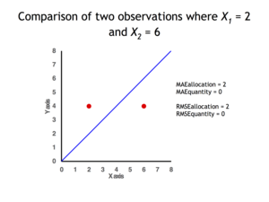
2 data points for which Quantity Disagreement is 0 and Allocation Disagreement is 2 for both MAE and RMSE
It is possible to express MAE as the sum of two components: Quantity Disagreement and Allocation Disagreement. Quantity Disagreement is the absolute value of the Mean Error given by:[4]

Allocation Disagreement is MAE minus Quantity Disagreement.
It is also possible to identify the types of difference by looking at an  plot. Quantity difference exists when the average of the X values does not equal the average of the Y values. Allocation difference exists if and only if points reside on both sides of the identity line.[4][5]
[edit]
The mean absolute error is one of a number of ways of comparing forecasts with their eventual outcomes. Well-established alternatives are the mean absolute scaled error (MASE) and the mean squared error. These all summarize performance in ways that disregard the direction of over- or under- prediction; a measure that does place emphasis on this is the mean signed difference.
Where a prediction model is to be fitted using a selected performance measure, in the sense that the least squares approach is related to the mean squared error, the equivalent for mean absolute error is least absolute deviations.
MAE is not identical to root-mean square error (RMSE), although some researchers report and interpret it that way. MAE is conceptually simpler and also easier to interpret than RMSE: it is simply the average absolute vertical or horizontal distance between each point in a scatter plot and the Y=X line. In other words, MAE is the average absolute difference between X and Y. Furthermore, each error contributes to MAE in proportion to the absolute value of the error. This is in contrast to RMSE which involves squaring the differences, so that a few large differences will increase the RMSE to a greater degree than the MAE.[4] See the example above for an illustration of these differences.
Optimality property[edit]
The mean absolute error of a real variable c with respect to the random variable X is

Provided that the probability distribution of X is such that the above expectation exists, then m is a median of X if and only if m is a minimizer of the mean absolute error with respect to X.[6] In particular, m is a sample median if and only if m minimizes the arithmetic mean of the absolute deviations.[7]
More generally, a median is defined as a minimum of

as discussed at Multivariate median (and specifically at Spatial median).
This optimization-based definition of the median is useful in statistical data-analysis, for example, in k-medians clustering.
Proof of optimality[edit]
Statement: The classifier minimising  is
is  .
.
Proof:
The Loss functions for classification is
![{displaystyle {begin{aligned}L&=mathbb {E} [|y-a||X=x]\&=int _{-infty }^{infty }|y-a|f_{Y|X}(y),dy\&=int _{-infty }^{a}(a-y)f_{Y|X}(y),dy+int _{a}^{infty }(y-a)f_{Y|X}(y),dy\end{aligned}}}](https://wikimedia.org/api/rest_v1/media/math/render/svg/7e953e54457072620a7c2764db0801f69c4e883d)
Differentiating with respect to a gives

This means

Hence

See also[edit]
- Least absolute deviations
- Mean absolute percentage error
- Mean percentage error
- Symmetric mean absolute percentage error
References[edit]
- ^ Willmott, Cort J.; Matsuura, Kenji (December 19, 2005). «Advantages of the mean absolute error (MAE) over the root mean square error (RMSE) in assessing average model performance». Climate Research. 30: 79–82. doi:10.3354/cr030079.
- ^ «2.5 Evaluating forecast accuracy | OTexts». www.otexts.org. Retrieved 2016-05-18.
- ^ Hyndman, R. and Koehler A. (2005). «Another look at measures of forecast accuracy» [1]
- ^ a b c Pontius Jr., Robert Gilmore; Thontteh, Olufunmilayo; Chen, Hao (2008). «Components of information for multiple resolution comparison between maps that share a real variable». Environmental and Ecological Statistics. 15 (2): 111–142. doi:10.1007/s10651-007-0043-y. S2CID 21427573.
- ^ Willmott, C. J.; Matsuura, K. (January 2006). «On the use of dimensioned measures of error to evaluate the performance of spatial interpolators». International Journal of Geographical Information Science. 20: 89–102. doi:10.1080/13658810500286976. S2CID 15407960.
- ^ Stroock, Daniel (2011). Probability Theory. Cambridge University Press. pp. 43. ISBN 978-0-521-13250-3.
- ^ Nicolas, André (2012-02-25). «The Median Minimizes the Sum of Absolute Deviations (The $ {L}_{1} $ Norm)». StackExchange.
Introduction
With any machine learning project, it is essential to measure the performance of the model. What we need is a metric to quantify the prediction error in a way that is easily understandable to an audience without a strong technical background. For regression problems, the Mean Absolute Error (MAE) is just such a metric.
The mean absolute error is the average difference between the observations (true values) and model output (predictions). The sign of these differences is ignored so that cancellations between positive and negative values do not occur. If we didn’t ignore the sign, the MAE calculated would likely be far lower than the true difference between model and data.
Mathematically, the MAE is expressed as:
MAE = frac{1}{N}sum_i^N|y_{i,pred}-y_{i,true}|
where y_{pred} are the predicted values, y_{true} are the observations, and N is the total number of samples considered in the calculation.
Python Coding Example
I will work though an example here using Python. First let’s load in the required packages:
## imports ##
import numpy as np
from sklearn.metrics import mean_absolute_error
import matplotlib.pyplot as plt
We can now create a toy dataset. For this example, I’ll generate data using a sine curve with noise added:
## define two arrays: x & y ##
x_true = np.linspace(0,4*np.pi,50)
y_true = np.sin(x_true) + np.random.rand(x_true.shape[0])
We can now plot these data:
## plot the data ##
plt.plot(x_true,y_true)
plt.title('Sinusoidal Data with Noise')
plt.xlabel('x')
plt.ylabel('y')
plt.show()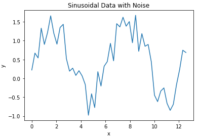
Now let’s assume we’ve built a model to predict the y values for every x in our toy dataset. Let’s plot the model output along with our data:
## plot the data & predictions ##
plt.plot(x_true,y_true)
plt.plot(x_true,y_pred)
plt.title('Sinusoidal Data with Noise + Predictions')
plt.xlabel('x')
plt.ylabel('y')
plt.legend(['y_true','y_pred'])
plt.show()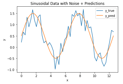
It’s evident that the model follows the general trend in the data, but there are differences. How can we quantify how large the differences are between the model predictions and data? Let’s address this by calculating the MAE, using the function available from scikit-learn:
## compute the mae ##
mae = mean_absolute_error(y_true,y_pred)
print("The mean absolute error is: {:.2f}".format(mae))
The mean absolute error is: 0.27
We find that the MAE is 0.27, giving us a measure of how accurate our model is for these data. We can plot these results with error bars superimposed on our model prediction values:
## plot the data & predictions with the mae ##
plt.plot(x_true,y_true)
plt.errorbar(x_true,y_pred,mae)
plt.title('Sinusoidal Data with Noise + Predictions')
plt.xlabel('x')
plt.ylabel('y')
plt.legend(['y_true','y_pred'])
plt.show()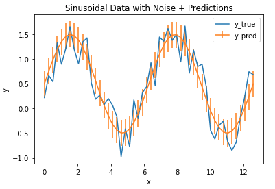
The vertical bars indicate the MAE calculated, and define a zone of uncertainty for our model predictions. We can see that this zone does encompass much of the random fluctuations in our data, and thus provides a reasonable estimate of the model accuracy.
The article contains a brief on various loss functions used in Neural networks.

What is a Loss function?
When you train Deep learning models, you feed data to the network, generate predictions, compare them with the actual values (the targets) and then compute what is known as a loss. This loss essentially tells you something about the performance of the network: the higher it is, the worse your network performs overall.
Loss functions are mainly classified into two different categories Classification loss and Regression Loss. Classification loss is the case where the aim is to predict the output from the different categorical values for example, if we have a dataset of handwritten images and the digit is to be predicted that lies between (0–9), in these kinds of scenarios classification loss is used.
Whereas if the problem is regression like predicting the continuous values for example, if need to predict the weather conditions or predicting the prices of houses on the basis of some features. In this type of case, Regression Loss is used.
In this article, we will focus on the most widely used loss functions in Neural networks.
-
Mean Absolute Error (L1 Loss)
-
Mean Squared Error (L2 Loss)
-
Huber Loss
-
Cross-Entropy(a.k.a Log loss)
-
Relative Entropy(a.k.a Kullback–Leibler divergence)
-
Squared Hinge
Mean Absolute Error (MAE)
Mean absolute error (MAE) also called L1 Loss is a loss function used for regression problems. It represents the difference between the original and predicted values extracted by averaging the absolute difference over the data set.

MAE is not sensitive towards outliers and is given several examples with the same input feature values, and the optimal prediction will be their median target value. This should be compared with Mean Squared Error, where the optimal prediction is the mean. A disadvantage of MAE is that the gradient magnitude is not dependent on the error size, only on the sign of y — ŷ which leads to that the gradient magnitude will be large even when the error is small, which in turn can lead to convergence problems.
When to use it?
Use Mean absolute error when you are doing regression and don’t want outliers to play a big role. It can also be useful if you know that your distribution is multimodal, and it’s desirable to have predictions at one of the modes, rather than at the mean of them.
Example: When doing image reconstruction, MAE encourages less blurry images compared to MSE. This is used for example in the paper Image-to-Image Translation with Conditional Adversarial Networks by Isola et al.
Mean Squared Error (MSE)
Mean Squared Error (MSE) also called L2 Loss is also a loss function used for regression. It represents the difference between the original and predicted values extracted by squared the average difference over the data set.

MSE is sensitive towards outliers and given several examples with the same input feature values, the optimal prediction will be their mean target value. This should be compared with Mean Absolute Error, where the optimal prediction is the median. MSE is thus good to use if you believe that your target data, conditioned on the input, is normally distributed around a mean value, and when it’s important to penalize outliers extra much.
When to use it?
Use MSE when doing regression, believing that your target, conditioned on the input, is normally distributed, and want large errors to be significantly (quadratically) more penalized than small ones.
Example: You want to predict future house prices. The price is a continuous value, and therefore we want to do regression. MSE can here be used as the loss function.
Calculate MAE and MSE using Python
Original target data is denoted by y and predicted label is denoted by (Ŷ) Yhat are the main sources to evaluate the model.
import math
import numpy as np
import matplotlib.pyplot as plt
y = np.array([-3, -1, -2, 1, -1, 1, 2, 1, 3, 4, 3, 5])
yhat = np.array([-2, 1, -1, 0, -1, 1, 2, 2, 3, 3, 3, 5])
x = list(range(len(y)))
#We can visualize them in a plot to check the difference visually.
plt.figure(figsize=(9, 5))
plt.scatter(x, y, color="red", label="original")
plt.plot(x, yhat, color="green", label="predicted")
plt.legend()
plt.show()

# calculate MSE
d = y - yhat
mse_f = np.mean(d**2)
print("Mean square error:",mse_f)
Mean square error: 0.75
# calculate MAE
mae_f = np.mean(abs(d))
print("Mean absolute error:",mae_f)
Mean absolute error: 0.5833333333333334
Huber Loss
Huber Loss is typically used in regression problems. It’s less sensitive to outliers than the MSE as it treats error as square only inside an interval.
Consider an example where we have a dataset of 100 values we would like our model to be trained to predict. Out of all that data, 25% of the expected values are 5 while the other 75% are 10.
An MSE loss wouldn’t quite do the trick, since we don’t really have “outliers”; 25% is by no means a small fraction. On the other hand, we don’t necessarily want to weigh that 25% too low with an MAE. Those values of 5 aren’t close to the median (10 — since 75% of the points have a value of 10), but they’re also not really outliers.
This is where the Huber Loss Function comes into play.
The Huber Loss offers the best of both worlds by balancing the MSE and MAE together. We can define it using the following piecewise function:

Here, (𝛿) delta → hyperparameter defines the range for MAE and MSE.
In simple terms, the above radically says is: for loss values less than (𝛿) delta, use the MSE; for loss values greater than delta, use the MAE. This way Huber loss provides the best of both MAE and MSE.
Set delta to the value of the residual for the data points, you trust.
import numpy as np
import matplotlib.pyplot as plt

def huber(a, delta):
  value = np.where(np.abs(a)<delta, .5*a**2, delta*(np.abs(a) - .5*delta))
  deriv = np.where(np.abs(a)<delta, a, np.sign(a)*delta)
  return value, deriv

h, d = huber(np.arange(-1, 1, .01), delta=0.2)

fig, ax = plt.subplots(1)
ax.plot(h, label='loss value')
ax.plot(d, label='loss derivative')
ax.grid(True)
ax.legend()

In the above figure, you can see how the derivative is a constant for abs(a)>delta
In TensorFlow 2 and Keras, Huber loss can be added to the compile step of your model.
model.compile(loss=tensorflow.keras.losses.Huber(delta=1.5), optimizer='adam', metrics=['mean_absolute_error'])
When to use Huber Loss?
As we already know Huber loss has both MAE and MSE. So when we think higher weightage should not be given to outliers, then set your loss function as Huber loss. We need to manually define is the (𝛿) delta value. Generally, some iterations are needed with the respective algorithm used to find the correct delta value.
Cross-Entropy Loss(a.k.a Log loss)
The concept of cross-entropy traces back into the field of Information Theory where Claude Shannon introduced the concept of entropy in 1948. Before diving into the Cross-Entropy loss function, let us talk about Entropy.
Entropy has roots in physics — it is a measure of disorder, or unpredictability, in a system.
For instance, consider below figure two gases in a box: initially, the system has low entropy, in that the two gasses are completely separable(skewed distribution); after some time, however, the gases blend(distribution where events have equal probability) so the system’s entropy increases. It is said that in an isolated system, the entropy never decreases — the chaos never dims down without external influence.

Entropy
For p(x) — probability distribution and a random variable X, entropy is defined as follows:

Reason for the Negative sign: log(p(x))<0 for all p(x) in (0,1) . p(x) is a probability distribution and therefore the values must range between 0 and 1.

A plot of log(x). For x values between 0 and 1, log(x) <0 (is negative).
Cross-Entropy loss is also called logarithmic loss, log loss, or logistic loss. Each predicted class probability is compared to the actual class desired output 0 or 1 and a score/loss is calculated that penalizes the probability based on how far it is from the actual expected value. The penalty is logarithmic in nature yielding a large score for large differences close to 1 and small score for small differences tending to 0.
Cross-Entropy is expressed by the equation;

Where x represents the predicted results by ML algorithm, p(x) is the probability distribution of “true” label from training samples and q(x) depicts the estimation of the ML algorithm.
Cross-entropy loss measures the performance of a classification model whose output is a probability value between 0 and 1. Cross-entropy loss increases as the predicted probability diverge from the actual label. So predicting a probability of .012 when the actual observation label is 1 would be bad and result in a high loss value. A perfect model would have a log loss of 0.

The graph above shows the range of possible loss values given a true observation. As the predicted probability approaches 1, log loss slowly decreases. As the predicted probability decreases, however, the log loss increases rapidly. Log loss penalizes both types of errors, but especially those predictions that are confident and wrong!
The cross-entropy method is a Monte Carlo technique for significance optimization and sampling.
Binary Cross-Entropy
Binary cross-entropy is a loss function that is used in binary classification tasks. These are tasks that answer a question with only two choices (yes or no, A or B, 0 or 1, left or right).
In binary classification, where the number of classes M equals 2, cross-entropy can be calculated as:

Sigmoid is the only activation function compatible with the binary cross-entropy loss function. You must use it on the last block before the target block.
The binary cross-entropy needs to compute the logarithms of Ŷi and (1-Ŷi), which only exist if Ŷi is between 0 and 1. The softmax activation function is the only one to guarantee that the output is within this range.
Categorical Cross-Entropy
Categorical cross-entropy is a loss function that is used in multi-class classification tasks. These are tasks where an example can only belong to one out of many possible categories, and the model must decide which one.
Formally, it is designed to quantify the difference between two probability distributions.
If 𝑀>2 (i.e. multiclass classification), we calculate a separate loss for each class label per observation and sum the result.

-
M — number of classes (dog, cat, fish)
-
log — the natural log
-
y — binary indicator (0 or 1) if class label c is the correct classification for observation o
-
p — predicted probability observation o is of class 𝑐
Softmax is the only activation function recommended to use with the categorical cross-entropy loss function.
Strictly speaking, the output of the model only needs to be positive so that the logarithm of every output value Ŷi exists. However, the main appeal of this loss function is for comparing two probability distributions. The softmax activation rescales the model output so that it has the right properties.
Sparse Categorical Cross-Entropy
sparse categorical cross-entropy has the same loss function as, categorical cross-entropy which we have mentioned above. The only difference is the format in which we mention 𝑌𝑖(i,e true labels).
If your Yi’s are one-hot encoded, use categorical_crossentropy. Examples for a 3-class classification: [1,0,0] , [0,1,0], [0,0,1]
But if your Yi’s are integers, use sparse_categorical_crossentropy. Examples for above 3-class classification problem: [1] , [2], [3]
The usage entirely depends on how you load your dataset. One advantage of using sparse categorical cross-entropy is it saves time in memory as well as computation because it simply uses a single integer for a class, rather than a whole vector.
Calculate Cross-Entropy Between Class Labels and Probabilities
The use of cross-entropy for classification often gives different specific names based on the number of classes.
Consider a two-class classification task with the following 10 actual class labels (P) and predicted class labels (Q).
# calculate cross entropy for classification problem
from math import log
from numpy import mean

# calculate cross entropy
def cross_entropy_funct(p, q):
 return -sum([p[i]*log(q[i]) for i in range(len(p))])

# define classification data p and q
p = [1, 1, 1, 1, 1, 0, 0, 0, 0, 0]
q = [0.7, 0.9, 0.8, 0.8, 0.6, 0.2, 0.1, 0.4, 0.1, 0.3]
# calculate cross entropy for each example
results = list()
for i in range(len(p)):
 # create the distribution for each event {0, 1}
 expected = [1.0 - p[i], p[i]]
 predicted = [1.0 - q[i], q[i]]
 # calculate cross entropy for the two events
 cross = cross_entropy_funct(expected, predicted)
 print('>[y=%.1f, yhat=%.1f] cross entropy: %.3f' % (p[i], q[i], cross))
 results.append(cross)

# calculate the average cross entropy
mean_cross_entropy = mean(results)
print('nAverage Cross Entropy: %.3f' % mean_cross_entropy)
Running the example prints the actual and predicted probabilities for each example. The final average cross-entropy loss across all examples is reported, in this case, as 0.272
>[y=1.0, yhat=0.7] cross entropy: 0.357
>[y=1.0, yhat=0.9] cross entropy: 0.105
>[y=1.0, yhat=0.8] cross entropy: 0.223
>[y=1.0, yhat=0.8] cross entropy: 0.223
>[y=1.0, yhat=0.6] cross entropy: 0.511
>[y=0.0, yhat=0.2] cross entropy: 0.223
>[y=0.0, yhat=0.1] cross entropy: 0.105
>[y=0.0, yhat=0.4] cross entropy: 0.511
>[y=0.0, yhat=0.1] cross entropy: 0.105
>[y=0.0, yhat=0.3] cross entropy: 0.357
Average Cross Entropy: 0.272
Relative Entropy(Kullback–Leibler divergence)
The Relative entropy (also called Kullback–Leibler divergence), is a method for measuring the similarity between two probability distributions. It was refined by Solomon Kullback and Richard Leibler for public release in 1951(paper), KL-Divergence aims to identify the divergence(separation or bifurcation) of a probability distribution given a baseline distribution. That is, for a target distribution, P, we compare a competing distribution, Q, by computing the expected value of the log-odds of the two distributions:
For distributions P and Q of a continuous random variable, the Kullback-Leibler divergence is computed as an integral:

If P and Q represent the probability distribution of a discrete random variable, the Kullback-Leibler divergence is calculated as a summation:

Also, with a little bit of work, we can show that the KL-Divergence is non-negative. It means, that the smallest possible value is zero (distributions are equal) and the maximum value is infinity. We procure infinity when P is defined in a region where Q can never exist. Therefore, it is a common assumption that both distributions exist on the same support.
The closer two distributions get to each other, the lower the loss becomes. In the following graph, the blue distribution is trying to model the green distribution. As the blue distribution comes closer and closer to the green one, the KL divergence loss will get closer to zero.
Lower the KL divergence value, the better we have matched the true distribution with our approximation.

Comparison of Blue and green distribution
The applications of KL-Divergence:
-
Primarily, it is used in Variational Autoencoders. These autoencoders learn to encode samples into a latent probability distribution and from this latent distribution, a sample can be drawn that can be fed to a decoder which outputs e.g. an image.
-
KL divergence can also be used in multiclass classification scenarios. These problems, which traditionally use the Softmax function and use one-hot encoded target data, are naturally suitable to KL divergence since Softmax “normalizes data into a probability distribution consisting of K probabilities proportional to the exponentials of the input numbers”
-
Delineating the relative (Shannon) entropy in information systems,
-
Randomness in continuous time-series.
Calculate KL-Divergence using Python

Consider a random variable with six events as different colors. We may have two different probability distributions for this variable; for example:
import numpy as np
import matplotlib.pyplot as plt

events = ['red', 'green', 'blue', 'black', 'yellow', 'orange']
p = [0.10, 0.30, 0.05, 0.90, 0.65, 0.21]
q = [0.70, 0.55, 0.15, 0.04, 0.25, 0.45]
Plot a histogram for each probability distribution, allowing the probabilities for each event to be directly compared.
# plot first distribution
plt.figure(figsize=(9, 5))
plt.subplot(2,1,1)
plt.bar(events, p, color ='green',align='center')
# plot second distribution
plt.subplot(2,1,2)
plt.bar(events, q,color ='green',align='center')
# show the plot
plt.show()
We can see that indeed the distributions are different.

Next, we can develop a function to calculate the KL divergence between the two distributions.
def kl_divergence(p, q):
    return sum(p[i] * np.log(p[i]/q[i]) for i in range(len(p)))

 # calculate (P || Q)
kl_pq = kl_divergence(p, q)
print('KL(P || Q): %.3f bits' % kl_pq)
# calculate (Q || P)
kl_qp = kl_divergence(q, p)
print('KL(Q || P): %.3f bits' % kl_qp)
KL(P || Q): 2.832 bits
KL(Q || P): 1.840 bits
Nevertheless, we can calculate the KL divergence using the rel_entr() SciPy function and confirm that our manual calculation is correct.
The rel_entr() function takes lists of probabilities across all events from each probability distribution as arguments and returns a list of divergences for each event. These can be summed to give the KL divergence.
from scipy.special import rel_entr

print("Using Scipy rel_entr function")

bo_1 = np.array(p)
bo_2 = np.array(q)

print('KL(P || Q): %.3f bits' % sum(rel_entr(bo_1,bo_2)))
print('KL(Q || P): %.3f bits' % sum(rel_entr(bo_2,bo_1)))
Using Scipy rel_entr function
KL(P || Q): 2.832 bits
KL(Q || P): 1.840 bits
Let us see how KL divergence can be used with Keras. It’s pretty simple, It just involves specifying it as the used loss function during the model compilation step:
# Compile the model model.compile(loss=keras.losses.kullback_leibler_divergence, optimizer=keras.optimizers.Adam(), metrics=[‘accuracy’])
Squared Hinge
The squared hinge loss is a loss function used for “maximum margin” binary classification problems. Mathematically it is defined as:

where ŷ is the predicted value and y is either 1 or -1.
Thus, the squared hinge loss → 0, when the true and predicted labels are the same and when ŷ≥ 1 (which is an indication that the classifier is sure that it’s the correct label).
The squared hinge loss → quadratically increasing with the error, when when the true and predicted labels are not the same or when ŷ< 1, even when the true and predicted labels are the same (which is an indication that the classifier is not sure that it’s the correct label).
As compared to traditional hinge loss(used in SVM) larger errors are punished more significantly, whereas smaller errors are punished slightly lighter.

Comparison between Hinge and Squared hinge loss
When to use Squared Hinge?
Use the Squared Hinge loss function on problems involving yes/no (binary) decisions. Especially, when you’re not interested in knowing how certain the classifier is about the classification. Namely, when you don’t care about the classification probabilities. Use in combination with the tanh() the activation function in the last layer of the neural network.
A typical application can be classifying email into ‘spam’ and ‘not spam’ and you’re only interested in the classification accuracy.
Let us see how Squared Hinge can be used with Keras. It’s pretty simple, It just involves specifying it as the used loss function during the model compilation step:
#Compile the model
model.compile(loss=squared_hinge, optimizer=tensorflow.keras.optimizers.Adam(lr=0.03), metrics=['accuracy'])
Feel free to connect me on LinkedIn for any query.
Thank you for reading this article, I hope you have found it useful.
References
https://www.machinecurve.com/index.php/2019/10/12/using-huber-loss-in-keras/
https://ml-cheatsheet.readthedocs.io/en/latest/loss_functions.html#:~:text=Cross%2Dentropy%20loss%2C%20or%20log,So%20predicting%20a%20probability%20of%20.
https://towardsdatascience.com/cross-entropy-loss-function-f38c4ec8643e
https://towardsdatascience.com/understanding-the-3-most-common-loss-functions-for-machine-learning-regression-23e0ef3e14d3
https://gobiviswa.medium.com/huber-error-loss-functions-3f2ac015cd45
https://www.datatechnotes.com/2019/10/accuracy-check-in-python-mae-mse-rmse-r.html
https://peltarion.com/knowledge-center/documentation/modeling-view/build-an-ai-model/loss-functions/
Anomaly detection
Patrick Schneider, Fatos Xhafa, in Anomaly Detection and Complex Event Processing over IoT Data Streams, 2022
Mean Absolute Error (MAE)
Mean absolute error (MAE) is a popular metric because, as with Root mean squared error (RMSE), see next subsection, the error value units match the predicted target value units. Unlike RMSE, the changes in MAE are linear and therefore intuitive. MSE and RMSE penalize larger errors more, inflating or increasing the mean error value due to the square of the error value. In MAE, different errors are not weighted more or less, but the scores increase linearly with the increase in errors. The MAE score is measured as the average of the absolute error values. The Absolute is a mathematical function that makes a number positive. Therefore, the difference between an expected value and a predicted value can be positive or negative and will necessarily be positive when calculating the MAE.
The MAE value can be calculated as follows:
(3.3)MAE=1n∑i=1n|y1−yiˆ|2
Read full chapter
URL:
https://www.sciencedirect.com/science/article/pii/B9780128238189000134
Characterization of forecast errors and benchmarking of renewable energy forecasts
Stefano Alessandrini, Simone Sperati, in Renewable Energy Forecasting, 2017
9.2.2.6 Golagh test case (Fig. 9.6)

Figure 9.6. Normalized mean absolute error (NMAE) for Golagh test case by Kariniotakis et al. (2004).
The NMAE values for the Golagh wind farm are less dependent on the forecast horizon than for the other wind farms. The range of variation of NMAE for 24 h horizon is 10%–16%, being comparable for longer forecast horizons.
The main evident conclusion coming out from these test cases is the strong dependence of predictability upon the terrain complexity. The performance of the prediction models is related to the complexity of the terrain. Fig. 9.7 represents the average value of the NMAE for the 12 h forecast horizon as a function of RIX index, for each test case.

Figure 9.7. Average normalized mean absolute error (NMAE) for 12 h forecast horizon versus RIX at each test case. Qualitative comparison over six wind farms: Tunø Knob (TUN), Klim (KLI), Wusterhusen (WUS), Sotavento (SOT), Golagh (GOL), Alaiz (ALA) by Kariniotakis et al. (2004).
Higher RIX values correspond to higher values of NMAE. It is also demonstrated that offshore wind farms (Tunø Knob) do not necessarily guarantee a better predictability than wind farms on flat terrain in similar climatic conditions.
Different performances between test cases could also be attributed to the use of different prediction models. In fact, the NWP used in the test case has been provided by the meteorological services of the different countries (Germany, Spain, Denmark, and Ireland). However, some of the cases, Alaiz and Sotavento, have the NWP obtained with the same model and the increase of NMAE with RIX still appears.
Read full chapter
URL:
https://www.sciencedirect.com/science/article/pii/B9780081005040000093
Validation methodologies
Ranadip Pal, in Predictive Modeling of Drug Sensitivity, 2017
4.2.1 Norm-Based Fitness Measures
MAE denotes the ratio of the 1 norm of the error vector Y−Y~ to the number of samples and is defined as
(4.1)MAE=1n∑i=1n|yi−y~i|
Mean bias error (MBE) captures the average bias in the prediction and is calculated as
(4.2)MBE=1n∑i=1n(y~i−yi)
MSE denotes the ratio of the square of the two norms of the error vector to the number of samples and is defined as
(4.3)MSE=1n∑i=1n(yi−y~i)2
Root mean square error (RMSE) denotes the square root of the MSE.
The MBE is usually not used as a measure of the model error as high individual errors in prediction can also produce a low MBE. MBE is primarily used to estimate the average bias in the model and to decide if any steps need to be taken to correct the model bias. The MBE, MAE, and RMSE are related by the following inequalities: MBE≤MAE≤RMSE≤nMAE. If any subsequent theoretical analysis is conducted on the error measure, MSE or RMSE is often preferred, as compared to MAE due to the ease of applying derivatives and other analytical measures. However, studies [2] have pointed out that RMSE is an inappropriate measure for average model performance, as it is a function of three characteristics: the variability in the error distribution, the square root of the number of error samples, and the average error magnitude (MAE). Due to the squaring portion of RMSE, larger errors will have more impact on the MSE than smaller errors. Furthermore, the upper limit of RMSE (MAE≤RMSE≤nMAE) varies with n and can have different interpretations for different sample sizes.
Note that the above measures will have the same units as the variable to be predicted and thus cannot be compared for different variables that are scaled differently. The normalization of the error can be handled either as normalized versions described next or using measures such as correlation coefficients and R2.
NRMSE as used in [3] is defined as
(4.4)NRMSE=∑i=1n(yi−y~i)2∑i=1n(yi−y-)2
or it can be defined as ratio of the RMSE to the range of the data or mean of the data.
Read full chapter
URL:
https://www.sciencedirect.com/science/article/pii/B978012805274700004X
Renewable energy system for industrial internet of things model using fusion-AI
Anand Singh Rajawat, … Ankush Ghosh, in Applications of AI and IOT in Renewable Energy, 2022
6.6 Results analysis
We evaluate different AI algorithms on different IIoT based datasets. Dissimilar assessment metrics were used to examine the goodness of the AI-based model, such as mean absolute error, mean absolute percent error, mean squared error, and root mean squared logarithmic error. We similarly selected the state-of-the-art models for the assessment through the proposed Fusion AI-based model.
6.6.1 Mean absolute error
The mean absolute error (MAE) characterizes the alteration among the original and predictable values and is mined as the dataset’s total alteration mean.
MAE=1n∑i=1n|Yi−Yiˆ|
6.6.2 Mean squared error
The mean squared error (MSE) is the alteration between the original value and the predictable value. It is mined by forming the mean formed error of the dataset.
MSE=1n∑i=1n(Yi−Yiˆ)2
6.6.3 Root mean squared logarithmic error
The root mean squared logarithmic error (RMSLE).
RMSLE=1n∑i=1n(log(yiˆ+1)−log(yi+1))2
6.6.4 Mean absolute percent error
The mean absolute percent error (MAPE) is theamount of the accuracy of a prediction. It measures the size of the error (Fig. 6.5; Table 6.1).

Figure 6.5. Comparative analysis in term of accuracy.
Table 6.1. Evaluation metrics.
| Model name | MAE | MSE | Root mean square error | RMSLE |
|---|---|---|---|---|
| Support Vector Machines(SVM) | 45.6755 | 1176.765 | 65.6675 | 0.1487659 |
| Recurrent Neural Network(RNN) | 28.9875 | 765.345 | 32.7657 | 0.701233 |
| Long Short-term Memory(LSTM) | 26.7865 | 657.765 | 30.6754 | 0.645361 |
| Fusion Artificial Intelligence | 14.564 | 352.6785 | 19.5643 | 0.023456 |
MAPE=∑|A−F|A×100N
Read full chapter
URL:
https://www.sciencedirect.com/science/article/pii/B9780323916998000061
Model development and validation methodology
Yen-Hsiung Kiang, in Fuel Property Estimation and Combustion Process Characterization, 2018
2.9.1 The Use of Mean Absolute Percentage Error/Mean Bias Percentage Error and Mean Absolute Error/Mean Bias Error
In this book, the MAPE/MBPE and MAE/MPE are used selectively. The complete data population is used in the validation analyses.
For the MAE/MBE and MAPE/MBPE methods, there are basic selection criteria.
- 1.
-
If the value of data is large, e.g., higher heating values ranging from 1000 to 10,000, the use of MAPE/MBPE method is a better choice. The reason is that the value of MAE/MBE may be too big and lead to confusion. For example, for a data value of 10,000, the value for MAE is 500 and the corresponding value for MAPE is 5%, which is within good engineering tolerance. However, if the absolute value of 500 is used, it is quite large in an absolute sense and just leads to confusion.
- 2.
-
If the absolute value of data is small (e.g., the chlorine content in the fuels) ranging from 0.1% to 2%, MAPE/MBPE methods should not be used. MAE/MBE methods are to be used to avoid confusion. The reason is that when the real concentration of chlorine in the fuel is 0.3%, if the estimated value is 0.6%, in practical engineering point of view, the estimated value is good enough for the applications. However, when using MAPE method, the value of MAPE is 100%. This greatly enlarges the significance of error. Thus the MAPE/MBPE methods are not recommended in these cases.
- 3.
-
In this book, the following definitions are used. The “deviation” or “% deviation” means the percentage difference from the absolute data value. And, “difference” is the difference of absolute values. For example, for an absolute value of 50, the deviation of ±5% means the range is between 50+5% and 50–5%, or, between absolute values of 47.5 and 52.5. However, the difference of 5 means the range is between 50–5 and 50+5, or between absolute values of 45 and 55.
- 4.
-
In this book, both MAE and MBE as well as MAPE and MBPE are used for the validations of higher heating values. MAE and MBE are only used for the validations of concentrations of carbon, nitrogen, oxygen, nitrogen, sulfur, and chlorine.
Read full chapter
URL:
https://www.sciencedirect.com/science/article/pii/B9780128134733000027
Forecasting of renewable generation for applications in smart grid power systems
Debesh Shankar Tripathy, B. Rajanarayan Prusty, in Advances in Smart Grid Power System, 2021
2.5 Forecast evaluation
Before utilizing forecasts for any real-life applications, they must be evaluated and analyzed based on the type of forecast. Two essential things to keep in mind are the quality of the forecasts to accurately present future realizations by proper modeling of the process, and the value of the forecast derived by using them for decision-making [14]. The quality of forecasts is assessed quantitatively by validating them over a period whose data has not been used for building (identifying and learning/training) the model.
2.5.1 Evaluating point forecasts
Point forecasts are widely assessed by calculating the forecast error via the use of different error measures. The most popular error measures are root mean square error (RMSE) and mean absolute error (MAE), which are discussed below. Apart from these, a variety of other error measures are available: mean square error, mean bias error, mean absolute percentage error, etc.
2.5.1.1 Root mean square error
The RMSE between the ith observation, Yi, and the corresponding forecast Yˆi for n forecast instants is given as
(10.2)RMSE=1n∑i=1n(Yi−Yˆi)2.
2.5.1.2 Mean absolute error
MAE is given as
(10.3)MAE=1n∑i=1n|Yi−Yˆi|.
In Eq. (10.3), the terms have the same meanings as in Eq. (10.2).
Note: RMSE and MAE are used to assess point forecasts but also can be extended to the probabilistic framework by replacing the point forecast with a quantile forecast to get the error measure for the corresponding quantile. Then the errors across different quantiles can be averaged to get a single value.
2.5.2 Evaluating probabilistic forecasts
Probabilistic forecasts, such as quantile, interval, and density forecasts, have different measures for evaluating their quality. Quantile forecasts can be assessed by the quantile score (QS) [12], which uses the PL function to differentially weigh the quantiles. Measures to evaluate the interval forecast include the Winkler score (WS) [12], prediction interval coverage probability (PICP) [15], and prediction interval normalized average width (PINAW) [15], which assess coverage and interval widths. Continuous ranked probability score (CRPS) [15] is the most widely used measure to determine the reliability and sharpness of density forecasts.
2.5.2.1 Quantile score
The QS uses the PL as a measure for the error in quantile forecasts. The PL function is defined as
(10.4)PL(Yi,Yˆi,τ,τundefined)={(1−τ)(Yˆi,τ−Yi)ifYi<Yˆi,ττ(Yi−Yˆi,τ)if Yi≥Yˆi,τ.undefined
In Eq. (10.4), Yi is the ith observation, and Yˆi,τ is the τth quantile forecast of the ith observation. The QS is the average PL across the nq predicted quantiles across the forecast horizon n and is given as
(10.5)QS=1nnq∑i=1n∑undefinedj=1nqPL(Yi,Yˆi,τ,τundefined).undefined
In Eq. (10.5), j is an index variable that represents the number of the quantile forecast. A lower score indicates a better prediction of the quantiles. The QS helps to assess both the reliability and sharpness of the quantile forecasts.
2.5.2.2 Winkler score
The WS is used to assess the accuracy of the coverage as well as the interval width for the PIs. For a PI centered at the median with (1−α)100% nominal coverage, this score is defined as the mean across the forecast horizon of
(10.6)WS={ΔiifLi≤Yi≤UiΔi+2(Li−Yi)/αifYi<LiΔi+2(Yi−Ui)/αifYi>Ui.undefined
In Eq. (10.6), Li is the lower-bound quantile, Ui is the upper-bound quantile, and Δi=Ui−Li is the interval width for the ith observation. It penalizes observations for lying outside the PI and rewards narrower interval widths. Hence, a lower WS is an indication of a better PI.
2.5.2.3 Prediction interval coverage probability
The PICP helps to ensure whether the observed probability distribution is bounded within the PI. The PICP index is calculated by counting the fraction of the number of observations lying within the forecast PI. It is mathematically represented as
(10.7)PICP=1n∑i=1nɛi,
where ɛi is defined as
(10.8)ɛi={1ifYi∈[Li,Ui]0ifYi∉[Li,Ui].
In Eqs. (10.7) and (10.8), the terms have their usual meaning as defined earlier. A higher PICP is desirable, as it indicates that more observations lie within the constructed PI. PICP quantitatively expresses reliability. A valid PICP should always be greater than the nominal confidence level.
2.5.2.4 Prediction interval normalized average width
The sole use of PICP can sometimes be misleading due to concentrating only on coverage of the PIs. The widths of PIs also play a significant role in assessing their informativeness. The quantitative expression of PI width is provided by the PINAW, which is given below:
(10.9)PINAW=1nR∑i=1nΔi.undefined
In Eq. (10.9), Δi is the interval width as in Eq. (10.6), and R is the normalizing factor given by the difference between the maximum and minimum forecast values. Hence, combined use of PICP and PINAW is required for proper evaluation of PIs.
2.5.2.5 Continuous ranked probability score
The CRPS robustly measures the reliability and sharpness of the probabilistic forecast. It is analogous to the MAE for point forecasts because it reduces to the absolute error for the point forecasts, hence allowing comparison of probabilistic and point forecasts. Since it is a measure of the absolute error of the forecast distribution, a lower CRPS is preferable. It considers the entire distribution of the forecasts contrary to QS, which uses the PL to weigh the different quantiles asymmetrically. It can be expressed as below:
(10.10)CRPS(F,y)=∫−∞∞(F(u)−I{y≤u})2du=EF|Y−y|−12EF|Y−Y’|undefined}.
In Eq. (10.10), y is the observation, F(u) is the CDF of density forecasts, I is the Heaviside step function, and Y and Y′ are two random variables with F as the distribution function.
Read full chapter
URL:
https://www.sciencedirect.com/science/article/pii/B9780128243374000102
Intelligence-Based Health Recommendation System Using Big Data Analytics
Abhaya Kumar Sahoo, … Himansu Das, in Big Data Analytics for Intelligent Healthcare Management, 2019
9.4.2 Experimental Result Analysis
Here we compare the results in terms of MAE value among existing methods and the proposed HRS by analyzing the healthcare dataset. As we obtained a lower MAE value for our proposed approach, we can say that our approach is a useful healthcare recommendation system.
In Table 9.3, MAE values are shown for the healthcare dataset where 10,000 patient ratings for 500 doctors are divided among 5 parties. Here p represents a number of parties collaborating, which varies from 1 to 5 where p = 1 meaning that there is no collaboration and all parties are generating predictions individually. The p = 2 signifies that two parties are collaborating and likewise for p = 3, 4, or 5. Fig. 9.7 depicts that MAE value is lower when all parties are collaborating, that is, p = 5. The lower the MAE value, the higher the accuracy. By using a collaborative-based filtering technique on the proposed HRS, we achieve lower MAE values and high accuracy when compared to existing approaches.
Table 9.3. Comparison Among Existing Approaches and Proposed HRS
| Contribution | Average MAE Values (Patients) | Average MAE Values (Doctors) |
|---|---|---|
| Yakut and Polat | 0.724 | 0.795 |
| Kaur et al. | 0.739 | 0.807 |
| Proposed HRS | 0.649 | 0.717 |

Fig. 9.7. Shows comparison among MAE and number of parties of proposed HRS.
Read full chapter
URL:
https://www.sciencedirect.com/science/article/pii/B978012818146100009X
Meta-Model Development
Bouzid Ait-Amir, … Abdelkhalak El Hami, in Embedded Mechatronic Systems 2 (Second Edition), 2020
6.5.3 Model comparison and validation
Once a model is built, the next step is validation. To choose one model or another two properties of the response surface are assessed as to their ability to match the experimental data and make predictions.
Certain mathematical criteria make it possible to test how the model results match the data. This is performed by the coefficient of determination R2, the adjusted R2 coefficient, or the study of the residues, etc.
The determination coefficient R2, which is the criterion generally used in linear regression to test how the model matches the data, is defined by:
[6.2]R2=1−∑i=1nyi−yi^2∑i=1nyi−y¯2
where y is an estimation of the average response and n is the number of points in the design of experiments.
The R2 criterion can be used to measure the percentage of the total variability of the response explained by the model. This coefficient should not be used to compare between various models, since it is highly dependent on the model used. Indeed, R2 increases when the number of terms goes up, even if all the predictors are not significant. To overcome this problem, the adjusted determination coefficient Radj2 can be used instead, defined by:
[6.3]Radj2=1−1n−p+1∑i=1nyi−yi^21n−1∑i=1nyi−yi¯2
where p represents the number of terms in the model (constant term not included). If Radj2 is expressed in terms of R2, it can be noted that Radj2 is always smaller than R2 and that the difference between these two coefficients increases with the number of predictors. Radj2 is, therefore, a compromise between a model which faithfully represents the variability of the response and a model which is not too rich in predictors.
Some methods have underlying hypotheses on the residuals ε^1,…,ε^n. For instance, for regression, the residuals are assumed to be centered. A residual analysis may be useful to compare the information provided by the determination coefficients.
Once the ability of the model to match the experimental data is checked, a second diagnosis is performed to check the ability of the adjusted surface to perform predictions. The experimental design space represents only a small domain of the possible values for the explanatory variables, whereas the adjusted model must be able to construct an approximate value of the response at any point in the field of study. It is therefore necessary to study if the proposed model can be applied to the total field of study and thus provide accurate predictions.
This method consists in comparing the predictions of the model at points which differ from those of the design of experiments. In the case where the number of feasible simulations is not constrained, it is possible to define a set of test points on which the prediction error criteria (MAE, RMSE, etc.) are evaluated. If not, it is possible to use cross-validation techniques.
In order to study the predictive qualities of the model, it is assumed that there are a reasonable number of test points. The indicators proposed below generally measure the mismatch between the prediction calculated by the adjusted model and the value of the response given by the simulator.
The determination coefficient R2 evaluated over a test process (also known as external R2) gives an indication of the prediction ability of the meta-model. The value of R2 can be negative, meaning that the model creates variability in comparison to a model providing constant prediction mismatch.
The mean square error (MSE) corresponds to the mean of the square of the prediction errors (L2– criterion method):
[6.4]MSE=1m∑i=1nyi−yi^2
where m represents the number of data from the test set. This criterion measures the mean square error of the mismatch between the predicted results and the test data. A low MSE value means that the predicted values match the real values.
The root mean square error (RMSE) criterion can also be used. It is defined by: RMSE=MSE
The RMSE depends on the order of magnitude of the observed values. It may, therefore, vary significantly from one application to the next. There are two ways to solve this problem. The first solution is to center and reduce the response (which is the solution usually taken). The second solution is to consider the criteria as being relative both in terms of mean (RRM) and standard deviation (RRE) defined as follows:
[6.5]RRM=1m∑i=1myi−yi^yi
[6.6]RRE=Varyi−yi^yi
The mean absolute error (MAE) criterion (which corresponds to standard L1) is defined by:
[6.7]MAE=1m∑i=1myi−yi^
This criterion is similar to the RMSE coefficient. Nevertheless, it is more robust since it is less sensitive to extreme values than MSE.
All distance measurements (MSE, RMSE and MAE) are equivalent and make it possible to quantify how the approximated solutions match the simulated data. A small value for these criteria means that the estimated model is able to predict the values of the response of the more complex model.
Table 6.8. Comparison of MSE and MAE criteria results for two meta-models (PLS regression and Kriging) on three responses Cmix, PdC and BPR
| Cmix | PdC | BPR | ||
|---|---|---|---|---|
| PLS regression | MSE | 1.4 × 10− 4 | 2.6 × 10− 7 | 2.7 × 10− 2 |
| MAE | 1.4 × 10− 2 | 1.6 × 10− 2 | 2.2 × 10− 2 | |
| Kriging | MSE | 2×10− 5 | 1.2 × 10− 8 | 4.3 × 10− 4 |
| MAE | 5.4 × 10− 3 | 3.6 × 10− 3 | 2.6 × 10− 3 |
Read full chapter
URL:
https://www.sciencedirect.com/science/article/pii/B9781785481901500062
27th European Symposium on Computer Aided Process Engineering
Sarah E. Davis, … Mario R. Eden, in Computer Aided Chemical Engineering, 2017
5 Results and Discussion
Four performance measures, MaAE, MPE, RMSE, and MAE, were calculated for each challenge function and a “unique” surrogate model combination. A “unique” surrogate model was trained using each of the data sets, which were generated from each challenge function using LHS, Sobol and Halton sequences. The differences between the performance measures of “unique” surrogate models for each challenge function were not statistically significant. Therefore, the performance metrics of “unique” surrogate models of each challenge function were averaged for the comparisons presented in this section.
The comparisons of MaAE and MPE, and RMSE and MAE provided similar trends. Hence, the results are summarized in terms of MaAE and RMSE. Figure 1(a) portrays how the MaAE changes for challenge functions with different number of inputs for each surrogate model type in a box-plot format. For each surrogate model type and number of inputs, the central mark represents the median, the cross shows the mean, and the edges of the rectangles are the 25th and 75th percentiles. Where present, the whiskers represent the most extreme points that are not considered outliers, and the outliers are plotted as individual dots. Figure 1(b) gives a similar plot for RMSE; and Figures 1(c) and 1(d) show the box-plots for MaAE and RMSE grouped based on challenge function shapes.

Figure 1. Box plots of performance for different surrogate models. Change in (a) MaAE, (b) RMSE with the number of function inputs; and (c) MaAE and (d) RMSE with function shape.
Figure 1(a) reveals that the surrogate models developed using ALAMO yielded the lowest MaAE for functions with two and five inputs, and the ones developed using ANN and ELM the lowest MaAE for functions with four and 10 inputs. The performance of ANN, ALAMO, and ELM models are comparable for functions with three inputs. In terms of RMSE (Figure 1(b)), the models developed using ANNs consistently provided the lowest values for all functions, where the RMSEs of the models developed using ALAMO were comparable to the RMSEs of ANN models for functions with four and 10 inputs. Overall, these comparisons suggest that the models developed using ANNs and ALAMO have comparable accuracy for functions with different dimensions. However, it should be noted that the surrogate models generated by ALAMO are consistently simpler functions than ANN models.
When the performance of surrogate model types are compared based on the shape of the challenge functions, ANN models yielded the smallest RMSE for all function shapes (Figure 1(d)). However, when the models are compared based on MaAE, in general, models developed using ALAMO and ELM yielded lower MaAEs than the ANN models (Figure 1(c)). For example, ALAMO models yielded the lowest MaAE for bowl shaped functions, whereas ELM models for valley shaped functions. Nevertheless, Figures 1(c) and (d) suggest that ANN, ALAMO, and ELM models overall consistently provided more accurate representation of the input-output data sets than the surrogate model forms considered.
Read full chapter
URL:
https://www.sciencedirect.com/science/article/pii/B9780444639653500787
Sky-Imaging Systems for Short-Term Forecasting
Bryan Urquhart, … Jan Kleissl, in Solar Energy Forecasting and Resource Assessment, 2013
9.5.4 Error Metrics
To evaluate the forecast, mean bias error (MBE), mean absolute error (MAE), and root mean square error (RMSE) were computed over the given period during daylight hours (SZA < 80°). The sky imager generates a forecast every 30 s, whereas the plant reports power output every 1 s, so to compare the forecast to actual power production, a 30 s average of power output data centered on the image capture time was used. These error metrics were computed for each of the 31 forecast intervals out to a 15 min forecast horizon.
While the metrics used provide a numerical evaluation of forecast accuracy, they are difficult to assess without a baseline comparison. The use of persistence as a baseline forecast is especially useful for short term forecasts. To generate a persistence forecast for comparison, the plant’s aggregate normalized power was averaged for 1 min prior to forecast issue and was then applied to the remainder of the 15 min forecast window. Adjustments were made for changing solar geometry throughout the 15 min forecast window by computing the clear-sky GI for each of the 30 s intervals.
Read full chapter
URL:
https://www.sciencedirect.com/science/article/pii/B9780123971777000097