From Wikipedia, the free encyclopedia
In statistics, mean absolute error (MAE) is a measure of errors between paired observations expressing the same phenomenon. Examples of Y versus X include comparisons of predicted versus observed, subsequent time versus initial time, and one technique of measurement versus an alternative technique of measurement. MAE is calculated as the sum of absolute errors divided by the sample size:[1]

It is thus an arithmetic average of the absolute errors  , where
  is the prediction and
  the true value. Note that alternative formulations may include relative frequencies as weight factors. The mean absolute error uses the same scale as the data being measured. This is known as a scale-dependent accuracy measure and therefore cannot be used to make comparisons between series using different scales.[2] The mean absolute error is a common measure of forecast error in time series analysis,[3] sometimes used in confusion with the more standard definition of mean absolute deviation. The same confusion exists more generally.
Quantity disagreement and allocation disagreement[edit]
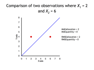
2 data points for which Quantity Disagreement is 0 and Allocation Disagreement is 2 for both MAE and RMSE
It is possible to express MAE as the sum of two components: Quantity Disagreement and Allocation Disagreement. Quantity Disagreement is the absolute value of the Mean Error given by:[4]

Allocation Disagreement is MAE minus Quantity Disagreement.
It is also possible to identify the types of difference by looking at an  plot. Quantity difference exists when the average of the X values does not equal the average of the Y values. Allocation difference exists if and only if points reside on both sides of the identity line.[4][5]
[edit]
The mean absolute error is one of a number of ways of comparing forecasts with their eventual outcomes. Well-established alternatives are the mean absolute scaled error (MASE) and the mean squared error. These all summarize performance in ways that disregard the direction of over- or under- prediction; a measure that does place emphasis on this is the mean signed difference.
Where a prediction model is to be fitted using a selected performance measure, in the sense that the least squares approach is related to the mean squared error, the equivalent for mean absolute error is least absolute deviations.
MAE is not identical to root-mean square error (RMSE), although some researchers report and interpret it that way. MAE is conceptually simpler and also easier to interpret than RMSE: it is simply the average absolute vertical or horizontal distance between each point in a scatter plot and the Y=X line. In other words, MAE is the average absolute difference between X and Y. Furthermore, each error contributes to MAE in proportion to the absolute value of the error. This is in contrast to RMSE which involves squaring the differences, so that a few large differences will increase the RMSE to a greater degree than the MAE.[4] See the example above for an illustration of these differences.
Optimality property[edit]
The mean absolute error of a real variable c with respect to the random variable X is

Provided that the probability distribution of X is such that the above expectation exists, then m is a median of X if and only if m is a minimizer of the mean absolute error with respect to X.[6] In particular, m is a sample median if and only if m minimizes the arithmetic mean of the absolute deviations.[7]
More generally, a median is defined as a minimum of

as discussed at Multivariate median (and specifically at Spatial median).
This optimization-based definition of the median is useful in statistical data-analysis, for example, in k-medians clustering.
Proof of optimality[edit]
Statement: The classifier minimising  is
is  .
.
Proof:
The Loss functions for classification is
![{displaystyle {begin{aligned}L&=mathbb {E} [|y-a||X=x]\&=int _{-infty }^{infty }|y-a|f_{Y|X}(y),dy\&=int _{-infty }^{a}(a-y)f_{Y|X}(y),dy+int _{a}^{infty }(y-a)f_{Y|X}(y),dy\end{aligned}}}](https://wikimedia.org/api/rest_v1/media/math/render/svg/7e953e54457072620a7c2764db0801f69c4e883d)
Differentiating with respect to a gives

This means

Hence

See also[edit]
- Least absolute deviations
- Mean absolute percentage error
- Mean percentage error
- Symmetric mean absolute percentage error
References[edit]
- ^ Willmott, Cort J.; Matsuura, Kenji (December 19, 2005). «Advantages of the mean absolute error (MAE) over the root mean square error (RMSE) in assessing average model performance». Climate Research. 30: 79–82. doi:10.3354/cr030079.
- ^ «2.5 Evaluating forecast accuracy | OTexts». www.otexts.org. Retrieved 2016-05-18.
- ^ Hyndman, R. and Koehler A. (2005). «Another look at measures of forecast accuracy» [1]
- ^ a b c Pontius Jr., Robert Gilmore; Thontteh, Olufunmilayo; Chen, Hao (2008). «Components of information for multiple resolution comparison between maps that share a real variable». Environmental and Ecological Statistics. 15 (2): 111–142. doi:10.1007/s10651-007-0043-y. S2CID 21427573.
- ^ Willmott, C. J.; Matsuura, K. (January 2006). «On the use of dimensioned measures of error to evaluate the performance of spatial interpolators». International Journal of Geographical Information Science. 20: 89–102. doi:10.1080/13658810500286976. S2CID 15407960.
- ^ Stroock, Daniel (2011). Probability Theory. Cambridge University Press. pp. 43. ISBN 978-0-521-13250-3.
- ^ Nicolas, André (2012-02-25). «The Median Minimizes the Sum of Absolute Deviations (The $ {L}_{1} $ Norm)». StackExchange.
Для того чтобы модель линейной регрессии можно было применять на практике необходимо сначала оценить её качество. Для этих целей предложен ряд показателей, каждый из которых предназначен для использования в различных ситуациях и имеет свои особенности применения (линейные и нелинейные, устойчивые к аномалиям, абсолютные и относительные, и т.д.). Корректный выбор меры для оценки качества модели является одним из важных факторов успеха в решении задач анализа данных.
- Среднеквадратичная ошибка (Mean Squared Error)
- Корень из среднеквадратичной ошибки (Root Mean Squared Error)
- Среднеквадратичная ошибка в процентах (Mean Squared Percentage Error)
- Cредняя абсолютная ошибка (Mean Absolute Error)
- Средняя абсолютная процентная ошибка (Mean Absolute Percentage Error)
- Cимметричная средняя абсолютная процентная ошибка (Symmetric Mean Absolute Percentage Error)
- Средняя абсолютная масштабированная ошибка (Mean absolute scaled error)
- Средняя относительная ошибка (Mean Relative Error)
- Среднеквадратичная логарифмическая ошибка (Root Mean Squared Logarithmic Error
- R-квадрат
- Скорректированный R-квадрат
- Сравнение метрик
«Хорошая» аналитическая модель должна удовлетворять двум, зачастую противоречивым, требованиям — как можно лучше соответствовать данным и при этом быть удобной для интерпретации пользователем. Действительно, повышение соответствия модели данным как правило связано с её усложнением (в случае регрессии — увеличением числа входных переменных модели). А чем сложнее модель, тем ниже её интерпретируемость.
Поэтому при выборе между простой и сложной моделью последняя должна значимо увеличивать соответствие модели данным чтобы оправдать рост сложности и соответствующее снижение интерпретируемости. Если это условие не выполняется, то следует выбрать более простую модель.
Таким образом, чтобы оценить, насколько повышение сложности модели значимо увеличивает её точность, необходимо использовать аппарат оценки качества регрессионных моделей. Он включает в себя следующие меры:
- Среднеквадратичная ошибка (MSE).
- Корень из среднеквадратичной ошибки (RMSE).
- Среднеквадратичная ошибка в процентах (MSPE).
- Средняя абсолютная ошибка (MAE).
- Средняя абсолютная ошибка в процентах (MAPE).
- Cимметричная средняя абсолютная процентная ошибка (SMAPE).
- Средняя абсолютная масштабированная ошибка (MASE)
- Средняя относительная ошибка (MRE).
- Среднеквадратичная логарифмическая ошибка (RMSLE).
- Коэффициент детерминации R-квадрат.
- Скорректированный коэффициент детеминации.
Прежде чем перейти к изучению метрик качества, введём некоторые базовые понятия, которые нам в этом помогут. Для этого рассмотрим рисунок.
Рисунок 1. Линейная регрессия
Наклонная прямая представляет собой линию регрессии с переменной, на которой расположены точки, соответствующие предсказанным значениям выходной переменной widehat{y} (кружки синего цвета). Оранжевые кружки представляют фактические (наблюдаемые) значения y . Расстояния между ними и линией регрессии — это ошибка предсказания модели y-widehat{y} (невязка, остатки). Именно с её использованием вычисляются все приведённые в статье меры качества.
Горизонтальная линия представляет собой модель простого среднего, где коэффициент при независимой переменной x равен нулю, и остаётся только свободный член b, который становится равным среднему арифметическому фактических значений выходной переменной, т.е. b=overline{y}. Очевидно, что такая модель для любого значения входной переменной будет выдавать одно и то же значение выходной — overline{y}.
В линейной регрессии такая модель рассматривается как «бесполезная», хуже которой работает только «случайный угадыватель». Однако, она используется для оценки, насколько дисперсия фактических значений y относительно линии среднего, больше, чем относительно линии регрессии с переменной, т.е. насколько модель с переменной лучше «бесполезной».
MSE
Среднеквадратичная ошибка (Mean Squared Error) применяется в случаях, когда требуется подчеркнуть большие ошибки и выбрать модель, которая дает меньше именно больших ошибок. Большие значения ошибок становятся заметнее за счет квадратичной зависимости.
Действительно, допустим модель допустила на двух примерах ошибки 5 и 10. В абсолютном выражении они отличаются в два раза, но если их возвести в квадрат, получив 25 и 100 соответственно, то отличие будет уже в четыре раза. Таким образом модель, которая обеспечивает меньшее значение MSE допускает меньше именно больших ошибок.
MSE рассчитывается по формуле:
MSE=frac{1}{n}sumlimits_{i=1}^{n}(y_{i}-widehat{y}_{i})^{2},
где n — количество наблюдений по которым строится модель и количество прогнозов, y_{i} — фактические значение зависимой переменной для i-го наблюдения, widehat{y}_{i} — значение зависимой переменной, предсказанное моделью.
Таким образом, можно сделать вывод, что MSE настроена на отражение влияния именно больших ошибок на качество модели.
Недостатком использования MSE является то, что если на одном или нескольких неудачных примерах, возможно, содержащих аномальные значения будет допущена значительная ошибка, то возведение в квадрат приведёт к ложному выводу, что вся модель работает плохо. С другой стороны, если модель даст небольшие ошибки на большом числе примеров, то может возникнуть обратный эффект — недооценка слабости модели.
RMSE
Корень из среднеквадратичной ошибки (Root Mean Squared Error) вычисляется просто как квадратный корень из MSE:
RMSE=sqrt{frac{1}{n}sumlimits_{i=1}^{n}(y_{i}-widehat{y_{i}})^{2}}
MSE и RMSE могут минимизироваться с помощью одного и того же функционала, поскольку квадратный корень является неубывающей функцией. Например, если у нас есть два набора результатов работы модели, A и B, и MSE для A больше, чем MSE для B, то мы можем быть уверены, что RMSE для A больше RMSE для B. Справедливо и обратное: если MSE(A)<MSE(B), то и RMSE(A)<RMSE(B).
Следовательно, сравнение моделей с помощью RMSE даст такой же результат, что и для MSE. Однако с MSE работать несколько проще, поэтому она более популярна у аналитиков. Кроме этого, имеется небольшая разница между этими двумя ошибками при оптимизации с использованием градиента:
frac{partial RMSE}{partial widehat{y}_{i}}=frac{1}{2sqrt{MSE}}frac{partial MSE}{partial widehat{y}_{i}}
Это означает, что перемещение по градиенту MSE эквивалентно перемещению по градиенту RMSE, но с другой скоростью, и скорость зависит от самой оценки MSE. Таким образом, хотя RMSE и MSE близки с точки зрения оценки моделей, они не являются взаимозаменяемыми при использовании градиента для оптимизации.
Влияние каждой ошибки на RMSE пропорционально величине квадрата ошибки. Поэтому большие ошибки оказывают непропорционально большое влияние на RMSE. Следовательно, RMSE можно считать чувствительной к аномальным значениям.
MSPE
Среднеквадратичная ошибка в процентах (Mean Squared Percentage Error) представляет собой относительную ошибку, где разность между наблюдаемым и фактическим значениями делится на наблюдаемое значение и выражается в процентах:
MSPE=frac{100}{n}sumlimits_{i=1}^{n}left ( frac{y_{i}-widehat{y}_{i}}{y_{i}} right )^{2}
Проблемой при использовании MSPE является то, что, если наблюдаемое значение выходной переменной равно 0, значение ошибки становится неопределённым.
MSPE можно рассматривать как взвешенную версию MSE, где вес обратно пропорционален квадрату наблюдаемого значения. Таким образом, при возрастании наблюдаемых значений ошибка имеет тенденцию уменьшаться.
MAE
Cредняя абсолютная ошибка (Mean Absolute Error) вычисляется следующим образом:
MAE=frac{1}{n}sumlimits_{i=1}^{n}left | y_{i}-widehat{y}_{i} right |
Т.е. MAE рассчитывается как среднее абсолютных разностей между наблюдаемым и предсказанным значениями. В отличие от MSE и RMSE она является линейной оценкой, а это значит, что все ошибки в среднем взвешены одинаково. Например, разница между 0 и 10 будет вдвое больше разницы между 0 и 5. Для MSE и RMSE, как отмечено выше, это не так.
Поэтому MAE широко используется, например, в финансовой сфере, где ошибка в 10 долларов должна интерпретироваться как в два раза худшая, чем ошибка в 5 долларов.
MAPE
Средняя абсолютная процентная ошибка (Mean Absolute Percentage Error) вычисляется следующим образом:
MAPE=frac{100}{n}sumlimits_{i=1}^{n}frac{left | y_{i}-widehat{y_{i}} right |}{left | y_{i} right |}
Эта ошибка не имеет размерности и очень проста в интерпретации. Её можно выражать как в долях, так и в процентах. Если получилось, например, что MAPE=11.4, то это говорит о том, что ошибка составила 11.4% от фактического значения.
SMAPE
Cимметричная средняя абсолютная процентная ошибка (Symmetric Mean Absolute Percentage Error) — это мера точности, основанная на процентных (или относительных) ошибках. Обычно определяется следующим образом:
SMAPE=frac{100}{n}sumlimits_{i=1}^{n}frac{left | y_{i}-widehat{y_{i}} right |}{(left | y_{i} right |+left | widehat{y}_{i} right |)/2}
Т.е. абсолютная разность между наблюдаемым и предсказанным значениями делится на полусумму их модулей. В отличие от обычной MAPE, симметричная имеет ограничение на диапазон значений. В приведённой формуле он составляет от 0 до 200%. Однако, поскольку диапазон от 0 до 100% гораздо удобнее интерпретировать, часто используют формулу, где отсутствует деление знаменателя на 2.
Одной из возможных проблем SMAPE является неполная симметрия, поскольку в разных диапазонах ошибка вычисляется неодинаково. Это иллюстрируется следующим примером: если y_{i}=100 и widehat{y}_{i}=110, то SMAPE=4.76, а если y_{i}=100 и widehat{y}_{i}=90, то SMAPE=5.26.
Ограничение SMAPE заключается в том, что, если наблюдаемое или предсказанное значение равно 0, ошибка резко возрастет до верхнего предела (200% или 100%).
MASE
Средняя абсолютная масштабированная ошибка (Mean absolute scaled error) — это показатель, который позволяет сравнивать две модели. Если поместить MAE для новой модели в числитель, а MAE для исходной модели в знаменатель, то полученное отношение и будет равно MASE. Если значение MASE меньше 1, то новая модель работает лучше, если MASE равно 1, то модели работают одинаково, а если значение MASE больше 1, то исходная модель работает лучше, чем новая модель. Формула для расчета MASE имеет вид:
MASE=frac{MAE_{i}}{MAE_{j}}
MASE симметрична и устойчива к выбросам.
MRE
Средняя относительная ошибка (Mean Relative Error) вычисляется по формуле:
MRE=frac{1}{n}sumlimits_{i=1}^{n}frac{left | y_{i}-widehat{y}_{i}right |}{left | y_{i} right |}
Несложно увидеть, что данная мера показывает величину абсолютной ошибки относительно фактического значения выходной переменной (поэтому иногда эту ошибку называют также средней относительной абсолютной ошибкой, MRAE). Действительно, если значение абсолютной ошибки, скажем, равно 10, то сложно сказать много это или мало. Например, относительно значения выходной переменной, равного 20, это составляет 50%, что достаточно много. Однако относительно значения выходной переменной, равного 100, это будет уже 10%, что является вполне нормальным результатом.
Очевидно, что при вычислении MRE нельзя применять наблюдения, в которых y_{i}=0.
Таким образом, MRE позволяет более адекватно оценить величину ошибки, чем абсолютные ошибки. Кроме этого она является безразмерной величиной, что упрощает интерпретацию.
RMSLE
Среднеквадратичная логарифмическая ошибка (Root Mean Squared Logarithmic Error) представляет собой RMSE, вычисленную в логарифмическом масштабе:
RMSLE=sqrt{frac{1}{n}sumlimits_{i=1}^{n}(log(widehat{y}_{i}+1)-log{(y_{i}+1}))^{2}}
Константы, равные 1, добавляемые в скобках, необходимы чтобы не допустить обращения в 0 выражения под логарифмом, поскольку логарифм нуля не существует.
Известно, что логарифмирование приводит к сжатию исходного диапазона изменения значений переменной. Поэтому применение RMSLE целесообразно, если предсказанное и фактическое значения выходной переменной различаются на порядок и больше.
R-квадрат
Перечисленные выше ошибки не так просто интерпретировать. Действительно, просто зная значение средней абсолютной ошибки, скажем, равное 10, мы сразу не можем сказать хорошая это ошибка или плохая, и что нужно сделать чтобы улучшить модель.
В этой связи представляет интерес использование для оценки качества регрессионной модели не значения ошибок, а величину показывающую, насколько данная модель работает лучше, чем модель, в которой присутствует только константа, а входные переменные отсутствуют или коэффициенты регрессии при них равны нулю.
Именно такой мерой и является коэффициент детерминации (Coefficient of determination), который показывает долю дисперсии зависимой переменной, объяснённой с помощью регрессионной модели. Наиболее общей формулой для вычисления коэффициента детерминации является следующая:
R^{2}=1-frac{sumlimits_{i=1}^{n}(widehat{y}_{i}-y_{i})^{2}}{sumlimits_{i=1}^{n}({overline{y}}_{i}-y_{i})^{2}}
Практически, в числителе данного выражения стоит среднеквадратическая ошибка оцениваемой модели, а в знаменателе — модели, в которой присутствует только константа.
Главным преимуществом коэффициента детерминации перед мерами, основанными на ошибках, является его инвариантность к масштабу данных. Кроме того, он всегда изменяется в диапазоне от −∞ до 1. При этом значения близкие к 1 указывают на высокую степень соответствия модели данным. Очевидно, что это имеет место, когда отношение в формуле стремится к 0, т.е. ошибка модели с переменными намного меньше ошибки модели с константой. R^{2}=0 показывает, что между независимой и зависимой переменными модели имеет место функциональная зависимость.
Когда значение коэффициента близко к 0 (т.е. ошибка модели с переменными примерно равна ошибке модели только с константой), это указывает на низкое соответствие модели данным, когда модель с переменными работает не лучше модели с константой.
Кроме этого, бывают ситуации, когда коэффициент R^{2} принимает отрицательные значения (обычно небольшие). Это произойдёт, если ошибка модели среднего становится меньше ошибки модели с переменной. В этом случае оказывается, что добавление в модель с константой некоторой переменной только ухудшает её (т.е. регрессионная модель с переменной работает хуже, чем предсказание с помощью простой средней).
На практике используют следующую шкалу оценок. Модель, для которой R^{2}>0.5, является удовлетворительной. Если R^{2}>0.8, то модель рассматривается как очень хорошая. Значения, меньшие 0.5 говорят о том, что модель плохая.
Скорректированный R-квадрат
Основной проблемой при использовании коэффициента детерминации является то, что он увеличивается (или, по крайней мере, не уменьшается) при добавлении в модель новых переменных, даже если эти переменные никак не связаны с зависимой переменной.
В связи с этим возникают две проблемы. Первая заключается в том, что не все переменные, добавляемые в модель, могут значимо увеличивать её точность, но при этом всегда увеличивают её сложность. Вторая проблема — с помощью коэффициента детерминации нельзя сравнивать модели с разным числом переменных. Чтобы преодолеть эти проблемы используют альтернативные показатели, одним из которых является скорректированный коэффициент детерминации (Adjasted coefficient of determinftion).
Скорректированный коэффициент детерминации даёт возможность сравнивать модели с разным числом переменных так, чтобы их число не влияло на статистику R^{2}, и накладывает штраф за дополнительно включённые в модель переменные. Вычисляется по формуле:
R_{adj}^{2}=1-frac{sumlimits_{i=1}^{n}(widehat{y}_{i}-y_{i})^{2}/(n-k)}{sumlimits_{i=1}^{n}({overline{y}}_{i}-y_{i})^{2}/(n-1)}
где n — число наблюдений, на основе которых строится модель, k — количество переменных в модели.
Скорректированный коэффициент детерминации всегда меньше единицы, но теоретически может принимать значения и меньше нуля только при очень малом значении обычного коэффициента детерминации и большом количестве переменных модели.
Сравнение метрик
Резюмируем преимущества и недостатки каждой приведённой метрики в следующей таблице:
| Мера | Сильные стороны | Слабые стороны |
|---|---|---|
| MSE | Позволяет подчеркнуть большие отклонения, простота вычисления. | Имеет тенденцию занижать качество модели, чувствительна к выбросам. Сложность интерпретации из-за квадратичной зависимости. |
| RMSE | Простота интерпретации, поскольку измеряется в тех же единицах, что и целевая переменная. | Имеет тенденцию занижать качество модели, чувствительна к выбросам. |
| MSPE | Нечувствительна к выбросам. Хорошо интерпретируема, поскольку имеет линейный характер. | Поскольку вклад всех ошибок отдельных наблюдений взвешивается одинаково, не позволяет подчёркивать большие и малые ошибки. |
| MAPE | Является безразмерной величиной, поэтому её интерпретация не зависит от предметной области. | Нельзя использовать для наблюдений, в которых значения выходной переменной равны нулю. |
| SMAPE | Позволяет корректно работать с предсказанными значениями независимо от того больше они фактического, или меньше. | Приближение к нулю фактического или предсказанного значения приводит к резкому росту ошибки, поскольку в знаменателе присутствует как фактическое, так и предсказанное значения. |
| MASE | Не зависит от масштаба данных, является симметричной: положительные и отрицательные отклонения от фактического значения учитываются одинаково. Устойчива к выбросам. Позволяет сравнивать модели. | Сложность интерпретации. |
| MRE | Позволяет оценить величину ошибки относительно значения целевой переменной. | Неприменима для наблюдений с нулевым значением выходной переменной. |
| RMSLE | Логарифмирование позволяет сделать величину ошибки более устойчивой, когда разность между фактическим и предсказанным значениями различается на порядок и выше | Может быть затруднена интерпретация из-за нелинейности. |
| R-квадрат | Универсальность, простота интерпретации. | Возрастает даже при включении в модель бесполезных переменных. Плохо работает когда входные переменные зависимы. |
| R-квадрат скорр. | Корректно отражает вклад каждой переменной в модель. | Плохо работает, когда входные переменные зависимы. |
В данной статье рассмотрены наиболее популярные меры качества регрессионных моделей, которые часто используются в различных аналитических приложениях. Эти меры имеют свои особенности применения, знание которых позволит обоснованно выбирать и корректно применять их на практике.
Однако в литературе можно встретить и другие меры качества моделей регрессии, которые предлагаются различными авторами для решения конкретных задач анализа данных.
Другие материалы по теме:
Отбор переменных в моделях линейной регрессии
Репрезентативность выборочных данных
Логистическая регрессия и ROC-анализ — математический аппарат
В машинном обучении различают оценки качества для задачи классификации и регрессии. Причем оценка задачи классификации часто значительно сложнее, чем оценка регрессии.
Содержание
- 1 Оценки качества классификации
- 1.1 Матрица ошибок (англ. Сonfusion matrix)
- 1.2 Аккуратность (англ. Accuracy)
- 1.3 Точность (англ. Precision)
- 1.4 Полнота (англ. Recall)
- 1.5 F-мера (англ. F-score)
- 1.6 ROC-кривая
- 1.7 Precison-recall кривая
- 2 Оценки качества регрессии
- 2.1 Средняя квадратичная ошибка (англ. Mean Squared Error, MSE)
- 2.2 Cредняя абсолютная ошибка (англ. Mean Absolute Error, MAE)
- 2.3 Коэффициент детерминации
- 2.4 Средняя абсолютная процентная ошибка (англ. Mean Absolute Percentage Error, MAPE)
- 2.5 Корень из средней квадратичной ошибки (англ. Root Mean Squared Error, RMSE)
- 2.6 Cимметричная MAPE (англ. Symmetric MAPE, SMAPE)
- 2.7 Средняя абсолютная масштабированная ошибка (англ. Mean absolute scaled error, MASE)
- 3 Кросс-валидация
- 4 Примечания
- 5 См. также
- 6 Источники информации
Оценки качества классификации
Матрица ошибок (англ. Сonfusion matrix)
Перед переходом к самим метрикам необходимо ввести важную концепцию для описания этих метрик в терминах ошибок классификации — confusion matrix (матрица ошибок).
Допустим, что у нас есть два класса и алгоритм, предсказывающий принадлежность каждого объекта одному из классов.
Рассмотрим пример. Пусть банк использует систему классификации заёмщиков на кредитоспособных и некредитоспособных. При этом первым кредит выдаётся, а вторые получат отказ. Таким образом, обнаружение некредитоспособного заёмщика () можно рассматривать как «сигнал тревоги», сообщающий о возможных рисках.
Любой реальный классификатор совершает ошибки. В нашем случае таких ошибок может быть две:
- Кредитоспособный заёмщик распознается моделью как некредитоспособный и ему отказывается в кредите. Данный случай можно трактовать как «ложную тревогу».
- Некредитоспособный заёмщик распознаётся как кредитоспособный и ему ошибочно выдаётся кредит. Данный случай можно рассматривать как «пропуск цели».
Несложно увидеть, что эти ошибки неравноценны по связанным с ними проблемам. В случае «ложной тревоги» потери банка составят только проценты по невыданному кредиту (только упущенная выгода). В случае «пропуска цели» можно потерять всю сумму выданного кредита. Поэтому системе важнее не допустить «пропуск цели», чем «ложную тревогу».
Поскольку с точки зрения логики задачи нам важнее правильно распознать некредитоспособного заёмщика с меткой , чем ошибиться в распознавании кредитоспособного, будем называть соответствующий исход классификации положительным (заёмщик некредитоспособен), а противоположный — отрицательным (заемщик кредитоспособен ). Тогда возможны следующие исходы классификации:
- Некредитоспособный заёмщик классифицирован как некредитоспособный, т.е. положительный класс распознан как положительный. Наблюдения, для которых это имеет место называются истинно-положительными (True Positive — TP).
- Кредитоспособный заёмщик классифицирован как кредитоспособный, т.е. отрицательный класс распознан как отрицательный. Наблюдения, которых это имеет место, называются истинно отрицательными (True Negative — TN).
- Кредитоспособный заёмщик классифицирован как некредитоспособный, т.е. имела место ошибка, в результате которой отрицательный класс был распознан как положительный. Наблюдения, для которых был получен такой исход классификации, называются ложно-положительными (False Positive — FP), а ошибка классификации называется ошибкой I рода.
- Некредитоспособный заёмщик распознан как кредитоспособный, т.е. имела место ошибка, в результате которой положительный класс был распознан как отрицательный. Наблюдения, для которых был получен такой исход классификации, называются ложно-отрицательными (False Negative — FN), а ошибка классификации называется ошибкой II рода.
Таким образом, ошибка I рода, или ложно-положительный исход классификации, имеет место, когда отрицательное наблюдение распознано моделью как положительное. Ошибкой II рода, или ложно-отрицательным исходом классификации, называют случай, когда положительное наблюдение распознано как отрицательное. Поясним это с помощью матрицы ошибок классификации:
-
Истинно-положительный (True Positive — TP) Ложно-положительный (False Positive — FP) Ложно-отрицательный (False Negative — FN) Истинно-отрицательный (True Negative — TN)
Здесь — это ответ алгоритма на объекте, а — истинная метка класса на этом объекте.
Таким образом, ошибки классификации бывают двух видов: False Negative (FN) и False Positive (FP).
P означает что классификатор определяет класс объекта как положительный (N — отрицательный). T значит что класс предсказан правильно (соответственно F — неправильно). Каждая строка в матрице ошибок представляет спрогнозированный класс, а каждый столбец — фактический класс.
 # код для матрицы ошибок
 # Пример классификатора, способного проводить различие между всего лишь двумя
 # классами, "пятерка" и "не пятерка" из набора рукописных цифр MNIST
 import numpy as np
 from sklearn.datasets import fetch_openml
 from sklearn.model_selection import cross_val_predict
 from sklearn.metrics import confusion_matrix
 from sklearn.linear_model import SGDClassifier
 mnist = fetch_openml('mnist_784', version=1)
 X, y = mnist["data"], mnist["target"]
 y = y.astype(np.uint8)
 X_train, X_test, y_train, y_test = X[:60000], X[60000:], y[:60000], y[60000:]
 y_train_5 = (y_train == 5) # True для всех пятерок, False для в сех остальных цифр. Задача опознать пятерки
 y_test_5 = (y_test == 5)
 sgd_clf = SGDClassifier(random_state=42) # классификатор на основе метода стохастического градиентного спуска (англ. Stochastic Gradient Descent SGD)
 sgd_clf.fit(X_train, y_train_5) # обучаем классификатор распозновать пятерки на целом обучающем наборе
 # Для расчета матрицы ошибок сначала понадобится иметь набор прогнозов, чтобы их можно было сравнивать с фактическими целями
 y_train_pred = cross_val_predict(sgd_clf, X_train, y_train_5, cv=3)
 print(confusion_matrix(y_train_5, y_train_pred))
 # array([[53892, 687],
 #        [ 1891, 3530]])
Безупречный классификатор имел бы только истинно-положительные и истинно отрицательные классификации, так что его матрица ошибок содержала бы ненулевые значения только на своей главной диагонали (от левого верхнего до правого нижнего угла):
 import numpy as np
 from sklearn.datasets import fetch_openml
 from sklearn.metrics import confusion_matrix
 mnist = fetch_openml('mnist_784', version=1)
 X, y = mnist["data"], mnist["target"]
 y = y.astype(np.uint8)
 X_train, X_test, y_train, y_test = X[:60000], X[60000:], y[:60000], y[60000:]
 y_train_5 = (y_train == 5) # True для всех пятерок, False для в сех остальных цифр. Задача опознать пятерки
 y_test_5 = (y_test == 5)
 y_train_perfect_predictions = y_train_5 # притворись, что мы достигли совершенства
 print(confusion_matrix(y_train_5, y_train_perfect_predictions))
 # array([[54579, 0],
 #        [ 0, 5421]])
Аккуратность (англ. Accuracy)
Интуитивно понятной, очевидной и почти неиспользуемой метрикой является accuracy — доля правильных ответов алгоритма:
Эта метрика бесполезна в задачах с неравными классами, что как вариант можно исправить с помощью алгоритмов сэмплирования и это легко показать на примере.
Допустим, мы хотим оценить работу спам-фильтра почты. У нас есть 100 не-спам писем, 90 из которых наш классификатор определил верно (True Negative = 90, False Positive = 10), и 10 спам-писем, 5 из которых классификатор также определил верно (True Positive = 5, False Negative = 5).
Тогда accuracy:
Однако если мы просто будем предсказывать все письма как не-спам, то получим более высокую аккуратность:
При этом, наша модель совершенно не обладает никакой предсказательной силой, так как изначально мы хотели определять письма со спамом. Преодолеть это нам поможет переход с общей для всех классов метрики к отдельным показателям качества классов.
 # код для для подсчета аккуратности:
 # Пример классификатора, способного проводить различие между всего лишь двумя
 # классами, "пятерка" и "не пятерка" из набора рукописных цифр MNIST
 import numpy as np
 from sklearn.datasets import fetch_openml
 from sklearn.model_selection import cross_val_predict
 from sklearn.metrics import accuracy_score
 from sklearn.linear_model import SGDClassifier
 mnist = fetch_openml('mnist_784', version=1)
 X, y = mnist["data"], mnist["target"]
 y = y.astype(np.uint8)
 X_train, X_test, y_train, y_test = X[:60000], X[60000:], y[:60000], y[60000:]
 y_train_5 = (y_train == 5) # True для всех пятерок, False для в сех остальных цифр. Задача опознать пятерки
 y_test_5 = (y_test == 5)
 sgd_clf = SGDClassifier(random_state=42) # классификатор на основе метода стохастического градиентного спуска (Stochastic Gradient Descent SGD)
 sgd_clf.fit(X_train, y_train_5) # обучаем классификатор распозновать пятерки на целом обучающем наборе
 y_train_pred = cross_val_predict(sgd_clf, X_train, y_train_5, cv=3)
 # print(confusion_matrix(y_train_5, y_train_pred))
 # array([[53892, 687]
 #        [ 1891, 3530]])
 print(accuracy_score(y_train_5, y_train_pred)) # == (53892 + 3530) / (53892 + 3530  + 1891 +687)

 # 0.9570333333333333
Точность (англ. Precision)
Точностью (precision) называется доля правильных ответов модели в пределах класса — это доля объектов действительно принадлежащих данному классу относительно всех объектов которые система отнесла к этому классу.
Именно введение precision не позволяет нам записывать все объекты в один класс, так как в этом случае мы получаем рост уровня False Positive.
Полнота (англ. Recall)
Полнота — это доля истинно положительных классификаций. Полнота показывает, какую долю объектов, реально относящихся к положительному классу, мы предсказали верно.
Полнота (recall) демонстрирует способность алгоритма обнаруживать данный класс вообще.
Имея матрицу ошибок, очень просто можно вычислить точность и полноту для каждого класса. Точность (precision) равняется отношению соответствующего диагонального элемента матрицы и суммы всей строки класса. Полнота (recall) — отношению диагонального элемента матрицы и суммы всего столбца класса. Формально:
Результирующая точность классификатора рассчитывается как арифметическое среднее его точности по всем классам. То же самое с полнотой. Технически этот подход называется macro-averaging.
 # код для для подсчета точности и полноты:
 # Пример классификатора, способного проводить различие между всего лишь двумя
 # классами, "пятерка" и "не пятерка" из набора рукописных цифр MNIST
 import numpy as np
 from sklearn.datasets import fetch_openml
 from sklearn.model_selection import cross_val_predict
 from sklearn.metrics import precision_score, recall_score
 from sklearn.linear_model import SGDClassifier
 mnist = fetch_openml('mnist_784', version=1)
 X, y = mnist["data"], mnist["target"]
 y = y.astype(np.uint8)
 X_train, X_test, y_train, y_test = X[:60000], X[60000:], y[:60000], y[60000:]
 y_train_5 = (y_train == 5) # True для всех пятерок, False для в сех остальных цифр. Задача опознать пятерки
 y_test_5 = (y_test == 5)
 sgd_clf = SGDClassifier(random_state=42) # классификатор на основе метода стохастического градиентного спуска (Stochastic Gradient Descent SGD)
 sgd_clf.fit(X_train, y_train_5) # обучаем классификатор распозновать пятерки на целом обучающем наборе
 y_train_pred = cross_val_predict(sgd_clf, X_train, y_train_5, cv=3)
 # print(confusion_matrix(y_train_5, y_train_pred))
 # array([[53892, 687]
 #        [ 1891, 3530]])
 print(precision_score(y_train_5, y_train_pred)) # == 3530 / (3530 + 687)
 print(recall_score(y_train_5, y_train_pred)) # == 3530 / (3530 + 1891)

 # 0.8370879772350012
 # 0.6511713705958311
F-мера (англ. F-score)
Precision и recall не зависят, в отличие от accuracy, от соотношения классов и потому применимы в условиях несбалансированных выборок.
Часто в реальной практике стоит задача найти оптимальный (для заказчика) баланс между этими двумя метриками. Понятно что чем выше точность и полнота, тем лучше. Но в реальной жизни максимальная точность и полнота не достижимы одновременно и приходится искать некий баланс. Поэтому, хотелось бы иметь некую метрику которая объединяла бы в себе информацию о точности и полноте нашего алгоритма. В этом случае нам будет проще принимать решение о том какую реализацию запускать в производство (у кого больше тот и круче). Именно такой метрикой является F-мера.
F-мера представляет собой гармоническое среднее между точностью и полнотой. Она стремится к нулю, если точность или полнота стремится к нулю.
Данная формула придает одинаковый вес точности и полноте, поэтому F-мера будет падать одинаково при уменьшении и точности и полноты. Возможно рассчитать F-меру придав различный вес точности и полноте, если вы осознанно отдаете приоритет одной из этих метрик при разработке алгоритма:
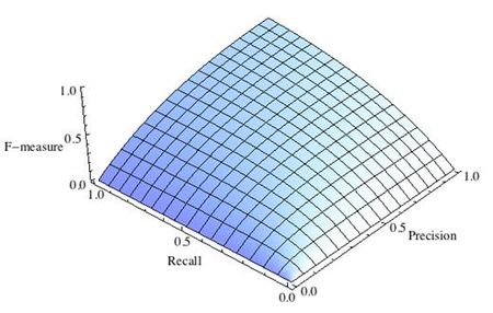
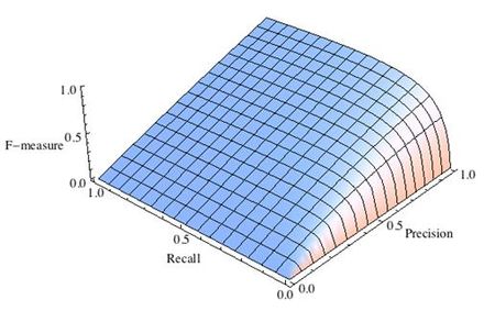
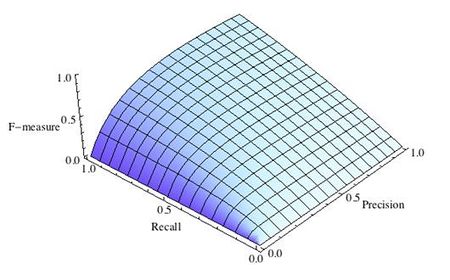
где принимает значения в диапазоне если вы хотите отдать приоритет точности, а при приоритет отдается полноте. При формула сводится к предыдущей и вы получаете сбалансированную F-меру (также ее называют ).
-

Рис.1 Сбалансированная F-мера,
-

Рис.2 F-мера c приоритетом точности,
-

Рис.3 F-мера c приоритетом полноты,
F-мера достигает максимума при максимальной полноте и точности, и близка к нулю, если один из аргументов близок к нулю.
F-мера является хорошим кандидатом на формальную метрику оценки качества классификатора. Она сводит к одному числу две других основополагающих метрики: точность и полноту. Имея «F-меру» гораздо проще ответить на вопрос: «поменялся алгоритм в лучшую сторону или нет?»
 # код для подсчета метрики F-mera:
 # Пример классификатора, способного проводить различие между всего лишь двумя
 # классами, "пятерка" и "не пятерка" из набора рукописных цифр MNIST
 import numpy as np
 from sklearn.datasets import fetch_openml
 from sklearn.model_selection import cross_val_predict
 from sklearn.linear_model import SGDClassifier
 from sklearn.metrics import f1_score
 mnist = fetch_openml('mnist_784', version=1)
 X, y = mnist["data"], mnist["target"]
 y = y.astype(np.uint8)
 X_train, X_test, y_train, y_test = X[:60000], X[60000:], y[:60000], y[60000:]
 y_train_5 = (y_train == 5) # True для всех пятерок, False для в сех остальных цифр. Задача опознать пятерки
 y_test_5 = (y_test == 5)
 sgd_clf = SGDClassifier(random_state=42) # классификатор на основе метода стохастического градиентного спуска (Stochastic Gradient Descent SGD)
 sgd_clf.fit(X_train, y_train_5) # обучаем классификатор распознавать пятерки на целом обучающем наборе
 y_train_pred = cross_val_predict(sgd_clf, X_train, y_train_5, cv=3)
 print(f1_score(y_train_5, y_train_pred))

 # 0.7325171197343846
ROC-кривая
Кривая рабочих характеристик (англ. Receiver Operating Characteristics curve).
Используется для анализа поведения классификаторов при различных пороговых значениях.
Позволяет рассмотреть все пороговые значения для данного классификатора.
Показывает долю ложно положительных примеров (англ. false positive rate, FPR) в сравнении с долей истинно положительных примеров (англ. true positive rate, TPR).
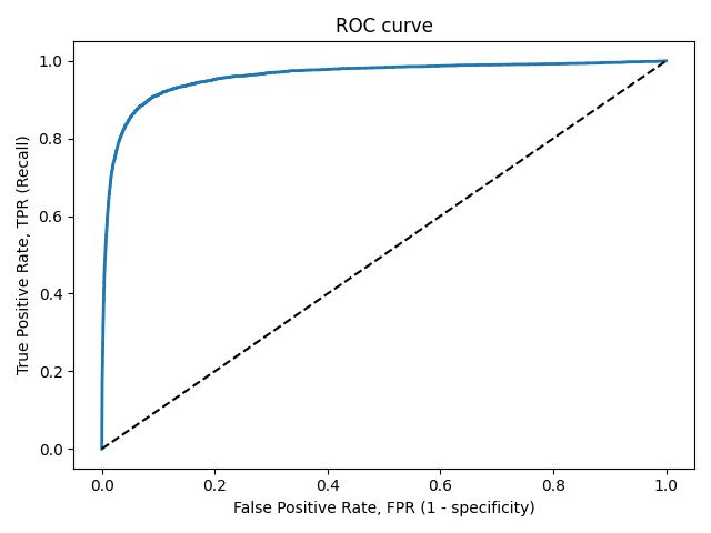
Доля FPR — это пропорция отрицательных образцов, которые были некорректно классифицированы как положительные.
- ,
где TNR — доля истинно отрицательных классификаций (англ. Тrие Negative Rate), представляющая собой пропорцию отрицательных образцов, которые были корректно классифицированы как отрицательные.
Доля TNR также называется специфичностью (англ. specificity). Следовательно, ROC-кривая изображает чувствительность (англ. seпsitivity), т.е. полноту, в сравнении с разностью 1 — specificity.
Прямая линия по диагонали представляет ROC-кривую чисто случайного классификатора. Хороший классификатор держится от указанной линии настолько далеко, насколько это
возможно (стремясь к левому верхнему углу).
Один из способов сравнения классификаторов предусматривает измерение площади под кривой (англ. Area Under the Curve — AUC). Безупречный классификатор будет иметь площадь под ROC-кривой (ROC-AUC), равную 1, тогда как чисто случайный классификатор — площадь 0.5.
 # Код отрисовки ROC-кривой
 # На примере классификатора, способного проводить различие между всего лишь двумя классами
 # "пятерка" и "не пятерка" из набора рукописных цифр MNIST
 from sklearn.metrics import roc_curve
 import matplotlib.pyplot as plt
 import numpy as np
 from sklearn.datasets import fetch_openml
 from sklearn.model_selection import cross_val_predict
 from sklearn.linear_model import SGDClassifier
 mnist = fetch_openml('mnist_784', version=1)
 X, y = mnist["data"], mnist["target"]
 y = y.astype(np.uint8)
 X_train, X_test, y_train, y_test = X[:60000], X[60000:], y[:60000], y[60000:]
 y_train_5 = (y_train == 5)  # True для всех пятерок, False для в сех остальных цифр. Задача опознать пятерки
 y_test_5 = (y_test == 5)
 sgd_clf = SGDClassifier(random_state=42) # классификатор на основе метода стохастического градиентного спуска (Stochastic Gradient Descent SGD)
 sgd_clf.fit(X_train, y_train_5) # обучаем классификатор распозновать пятерки на целом обучающем наборе
 y_train_pred = cross_val_predict(sgd_clf, X_train, y_train_5, cv=3)
 y_scores = cross_val_predict(sgd_clf, X_train, y_train_5, cv=3, method="decision_function")
 fpr, tpr, thresholds = roc_curve(y_train_5, y_scores)
 def plot_roc_curve(fpr, tpr, label=None):
     plt.plot(fpr, tpr, linewidth=2, label=label)
     plt.plot([0, 1], [0, 1], 'k--') # dashed diagonal
     plt.xlabel('False Positive Rate, FPR (1 - specificity)')
     plt.ylabel('True Positive Rate, TPR (Recall)')
     plt.title('ROC curve')
     plt.savefig("ROC.png")
 plot_roc_curve(fpr, tpr)
 plt.show()
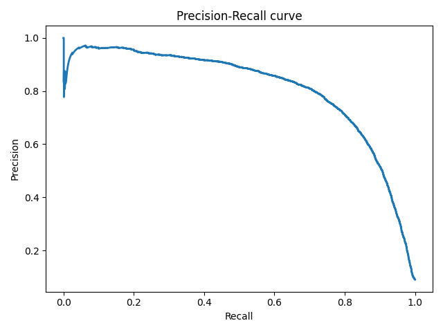
Precison-recall кривая
Чувствительность к соотношению классов.
Рассмотрим задачу выделения математических статей из множества научных статей. Допустим, что всего имеется 1.000.100 статей, из которых лишь 100 относятся к математике. Если нам удастся построить алгоритм , идеально решающий задачу, то его TPR будет равен единице, а FPR — нулю. Рассмотрим теперь плохой алгоритм, дающий положительный ответ на 95 математических и 50.000 нематематических статьях. Такой алгоритм совершенно бесполезен, но при этом имеет TPR = 0.95 и FPR = 0.05, что крайне близко к показателям идеального алгоритма.
Таким образом, если положительный класс существенно меньше по размеру, то AUC-ROC может давать неадекватную оценку качества работы алгоритма, поскольку измеряет долю неверно принятых объектов относительно общего числа отрицательных. Так, алгоритм , помещающий 100 релевантных документов на позиции с 50.001-й по 50.101-ю, будет иметь AUC-ROC 0.95.
Precison-recall (PR) кривая. Избавиться от указанной проблемы с несбалансированными классами можно, перейдя от ROC-кривой к PR-кривой. Она определяется аналогично ROC-кривой, только по осям откладываются не FPR и TPR, а полнота (по оси абсцисс) и точность (по оси ординат). Критерием качества семейства алгоритмов выступает площадь под PR-кривой (англ. Area Under the Curve — AUC-PR)
 # Код отрисовки Precison-recall кривой
 # На примере классификатора, способного проводить различие между всего лишь двумя классами
 # "пятерка" и "не пятерка" из набора рукописных цифр MNIST
 from sklearn.metrics import precision_recall_curve
 import matplotlib.pyplot as plt
 import numpy as np
 from sklearn.datasets import fetch_openml
 from sklearn.model_selection import cross_val_predict
 from sklearn.linear_model import SGDClassifier
 mnist = fetch_openml('mnist_784', version=1)
 X, y = mnist["data"], mnist["target"]
 y = y.astype(np.uint8)
 X_train, X_test, y_train, y_test = X[:60000], X[60000:], y[:60000], y[60000:]
 y_train_5 = (y_train == 5) # True для всех пятерок, False для в сех остальных цифр. Задача опознать пятерки
 y_test_5 = (y_test == 5)
 sgd_clf = SGDClassifier(random_state=42) # классификатор на основе метода стохастического градиентного спуска (Stochastic Gradient Descent SGD)
 sgd_clf.fit(X_train, y_train_5) # обучаем классификатор распозновать пятерки на целом обучающем наборе
 y_train_pred = cross_val_predict(sgd_clf, X_train, y_train_5, cv=3)
 y_scores = cross_val_predict(sgd_clf, X_train, y_train_5, cv=3, method="decision_function")
 precisions, recalls, thresholds = precision_recall_curve(y_train_5, y_scores)
 def plot_precision_recall_vs_threshold(precisions, recalls, thresholds):
     plt.plot(recalls, precisions, linewidth=2)
     plt.xlabel('Recall')
     plt.ylabel('Precision')
     plt.title('Precision-Recall curve')
     plt.savefig("Precision_Recall_curve.png")
 plot_precision_recall_vs_threshold(precisions, recalls, thresholds)
 plt.show()
Оценки качества регрессии
Наиболее типичными мерами качества в задачах регрессии являются
Средняя квадратичная ошибка (англ. Mean Squared Error, MSE)
MSE применяется в ситуациях, когда нам надо подчеркнуть большие ошибки и выбрать модель, которая дает меньше больших ошибок прогноза. Грубые ошибки становятся заметнее за счет того, что ошибку прогноза мы возводим в квадрат. И модель, которая дает нам меньшее значение среднеквадратической ошибки, можно сказать, что что у этой модели меньше грубых ошибок.
- и
Cредняя абсолютная ошибка (англ. Mean Absolute Error, MAE)
Среднеквадратичный функционал сильнее штрафует за большие отклонения по сравнению со среднеабсолютным, и поэтому более чувствителен к выбросам. При использовании любого из этих двух функционалов может быть полезно проанализировать, какие объекты вносят наибольший вклад в общую ошибку — не исключено, что на этих объектах была допущена ошибка при вычислении признаков или целевой величины.
Среднеквадратичная ошибка подходит для сравнения двух моделей или для контроля качества во время обучения, но не позволяет сделать выводов о том, на сколько хорошо данная модель решает задачу. Например, MSE = 10 является очень плохим показателем, если целевая переменная принимает значения от 0 до 1, и очень хорошим, если целевая переменная лежит в интервале (10000, 100000). В таких ситуациях вместо среднеквадратичной ошибки полезно использовать коэффициент детерминации —
Коэффициент детерминации
Коэффициент детерминации измеряет долю дисперсии, объясненную моделью, в общей дисперсии целевой переменной. Фактически, данная мера качества — это нормированная среднеквадратичная ошибка. Если она близка к единице, то модель хорошо объясняет данные, если же она близка к нулю, то прогнозы сопоставимы по качеству с константным предсказанием.
Средняя абсолютная процентная ошибка (англ. Mean Absolute Percentage Error, MAPE)
Это коэффициент, не имеющий размерности, с очень простой интерпретацией. Его можно измерять в долях или процентах. Если у вас получилось, например, что MAPE=11.4%, то это говорит о том, что ошибка составила 11,4% от фактических значений.
Основная проблема данной ошибки — нестабильность.
Корень из средней квадратичной ошибки (англ. Root Mean Squared Error, RMSE)
Примерно такая же проблема, как и в MAPE: так как каждое отклонение возводится в квадрат, любое небольшое отклонение может значительно повлиять на показатель ошибки. Стоит отметить, что существует также ошибка MSE, из которой RMSE как раз и получается путем извлечения корня.
Cимметричная MAPE (англ. Symmetric MAPE, SMAPE)
Средняя абсолютная масштабированная ошибка (англ. Mean absolute scaled error, MASE)
MASE является очень хорошим вариантом для расчета точности, так как сама ошибка не зависит от масштабов данных и является симметричной: то есть положительные и отрицательные отклонения от факта рассматриваются в равной степени.
Обратите внимание, что в MASE мы имеем дело с двумя суммами: та, что в числителе, соответствует тестовой выборке, та, что в знаменателе — обучающей. Вторая фактически представляет собой среднюю абсолютную ошибку прогноза. Она же соответствует среднему абсолютному отклонению ряда в первых разностях. Эта величина, по сути, показывает, насколько обучающая выборка предсказуема. Она может быть равна нулю только в том случае, когда все значения в обучающей выборке равны друг другу, что соответствует отсутствию каких-либо изменений в ряде данных, ситуации на практике почти невозможной. Кроме того, если ряд имеет тенденцию к росту либо снижению, его первые разности будут колебаться около некоторого фиксированного уровня. В результате этого по разным рядам с разной структурой, знаменатели будут более-менее сопоставимыми. Всё это, конечно же, является очевидными плюсами MASE, так как позволяет складывать разные значения по разным рядам и получать несмещённые оценки.
Недостаток MASE в том, что её тяжело интерпретировать. Например, MASE=1.21 ни о чём, по сути, не говорит. Это просто означает, что ошибка прогноза оказалась в 1.21 раза выше среднего абсолютного отклонения ряда в первых разностях, и ничего более.
Кросс-валидация
Хороший способ оценки модели предусматривает применение кросс-валидации (cкользящего контроля или перекрестной проверки).
В этом случае фиксируется некоторое множество разбиений исходной выборки на две подвыборки: обучающую и контрольную. Для каждого разбиения выполняется настройка алгоритма по обучающей подвыборке, затем оценивается его средняя ошибка на объектах контрольной подвыборки. Оценкой скользящего контроля называется средняя по всем разбиениям величина ошибки на контрольных подвыборках.
Примечания
- [1] Лекция «Оценивание качества» на www.coursera.org
- [2] Лекция на www.stepik.org о кросвалидации
- [3] Лекция на www.stepik.org о метриках качества, Precison и Recall
- [4] Лекция на www.stepik.org о метриках качества, F-мера
- [5] Лекция на www.stepik.org о метриках качества, примеры
См. также
- Оценка качества в задаче кластеризации
- Кросс-валидация
Источники информации
- [6] Соколов Е.А. Лекция линейная регрессия
- [7] — Дьяконов А. Функции ошибки / функционалы качества
- [8] — Оценка качества прогнозных моделей
- [9] — HeinzBr Ошибка прогнозирования: виды, формулы, примеры
- [10] — egor_labintcev Метрики в задачах машинного обучения
- [11] — grossu Методы оценки качества прогноза
- [12] — К.В.Воронцов, Классификация
- [13] — К.В.Воронцов, Скользящий контроль
What is mean absolute error (MAE)?
Mean absolute error, or MAE, measures the performance of a regression model. The mean absolute error is defined as the average of the all absolute differences between true and predicted values:
$$mathrm{MAE}=frac{1}{n}sum^{n-1}_{i=0}(|y_i-hat{y}_i|)$$
Where:
-
$n$ is the number of predicted values
-
$y_i$ is the actual true value of the $i$-th data
-
$hat{y}_i$ is the predicted value of the $i$-th data
A model with a high value of MAE means that its performance is subpar, while one a MAE of zero would indicate a perfect model without any error in its predictions.
Simple example to calculate mean absolute error (MAE)
Suppose we have three data points (1,3), (2,2) and (3,2). In order to predict the y-value given the x-value, we have built a simple linear model $hat{y}=x$, as shown in the diagram below:
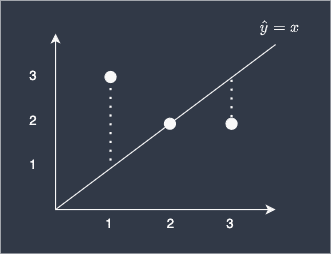
To get a measure of how good our model performs, we can compute the MAE like so:
$$begin{align*}
mathrm{MAE}&=frac{1}{3}left(|3-1|+|2-2|+|2-3|right)\
&=frac{1}{3}left(2+0+1right)\
&=1
end{align*}$$
This means that our predictions are off by one on average.
Why do we take the absolute value?
The reason is that the absolute value prevents positive and negative differences from cancelling each other out. As an example, consider the following example:
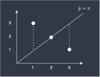
Suppose we computed the MAE without taking the absolute value:
$$begin{align*}
mathrm{MAE’}&=frac{1}{3}Big[(1-3)+(2-2)+(3-2)Big]\
&=frac{1}{3}left(-2+0+2right)\
&=0
end{align*}$$
As you can see, the negative and positive difference of the first and third data points have cancelled each other out. As a result, we end up with a MAE’ of 0, which is obviously misleading because we know that our model is not performing all that well. In order to avoid negative and positive differences to cancel each other out, MAE takes the absolute value of the difference.
Why isn’t mean absolute error (MAE) used as a cost function?
Most machine learning models «learn» by minimising the cost function. The mean absolute error is often not chosen as the cost function because the presence of the absolute value makes differentiation harder, which means the function is difficult to optimise. For this reason, mean squared error is typically chosen as the cost function to train machine learning models.
Computing mean absolute error (MAE) using Python’s Scikit-learn
To compute the mean absolute error given a list of true and predicted values:
from sklearn.metrics import mean_absolute_error
y_true = [2,6,5]
y_pred = [7,4,3]
mean_absolute_error(y_true, y_pred)
3.0
Setting multioutput
By default, multioutput='uniform_average', which returns a the global mean absolute error:
y_true = [[1,2],[3,4]]
y_pred = [[6,7],[9,8]]
mean_absolute_error(y_true, y_pred)
5.0
| title | date | categories | tags | |||||||||
|---|---|---|---|---|---|---|---|---|---|---|---|---|
|
About loss and loss functions |
2019-10-04 |
|
|
When you’re training supervised machine learning models, you often hear about a loss function that is minimized; that must be chosen, and so on.
The term cost function is also used equivalently.
But what is loss? And what is a loss function?
I’ll answer these two questions in this blog, which focuses on this optimization aspect of machine learning. We’ll first cover the high-level supervised learning process, to set the stage. This includes the role of training, validation and testing data when training supervised models.
Once we’re up to speed with those, we’ll introduce loss. We answer the question what is loss? However, we don’t forget what is a loss function? We’ll even look into some commonly used loss functions.
Let’s go! 😎
[toc]
[ad]
The high-level supervised learning process
Before we can actually introduce the concept of loss, we’ll have to take a look at the high-level supervised machine learning process. All supervised training approaches fall under this process, which means that it is equal for deep neural networks such as MLPs or ConvNets, but also for SVMs.
Let’s take a look at this training process, which is cyclical in nature.

Forward pass
We start with our features and targets, which are also called your dataset. This dataset is split into three parts before the training process starts: training data, validation data and testing data. The training data is used during the training process; more specificially, to generate predictions during the forward pass. However, after each training cycle, the predictive performance of the model must be tested. This is what the validation data is used for — it helps during model optimization.
Then there is testing data left. Assume that the validation data, which is essentially a statistical sample, does not fully match the population it describes in statistical terms. That is, the sample does not represent it fully and by consequence the mean and variance of the sample are (hopefully) slightly different than the actual population mean and variance. Hence, a little bias is introduced into the model every time you’ll optimize it with your validation data. While it may thus still work very well in terms of predictive power, it may be the case that it will lose its power to generalize. In that case, it would no longer work for data it has never seen before, e.g. data from a different sample. The testing data is used to test the model once the entire training process has finished (i.e., only after the last cycle), and allows us to tell something about the generalization power of our machine learning model.
The training data is fed into the machine learning model in what is called the forward pass. The origin of this name is really easy: the data is simply fed to the network, which means that it passes through it in a forward fashion. The end result is a set of predictions, one per sample. This means that when my training set consists of 1000 feature vectors (or rows with features) that are accompanied by 1000 targets, I will have 1000 predictions after my forward pass.
[ad]
Loss
You do however want to know how well the model performs with respect to the targets originally set. A well-performing model would be interesting for production usage, whereas an ill-performing model must be optimized before it can be actually used.
This is where the concept of loss enters the equation.
Most generally speaking, the loss allows us to compare between some actual targets and predicted targets. It does so by imposing a «cost» (or, using a different term, a «loss») on each prediction if it deviates from the actual targets.
It’s relatively easy to compute the loss conceptually: we agree on some cost for our machine learning predictions, compare the 1000 targets with the 1000 predictions and compute the 1000 costs, then add everything together and present the global loss.
Our goal when training a machine learning model?
To minimize the loss.
The reason why is simple: the lower the loss, the more the set of targets and the set of predictions resemble each other.
And the more they resemble each other, the better the machine learning model performs.
As you can see in the machine learning process depicted above, arrows are flowing backwards towards the machine learning model. Their goal: to optimize the internals of your model only slightly, so that it will perform better during the next cycle (or iteration, or epoch, as they are also called).
Backwards pass
When loss is computed, the model must be improved. This is done by propagating the error backwards to the model structure, such as the model’s weights. This closes the learning cycle between feeding data forward, generating predictions, and improving it — by adapting the weights, the model likely improves (sometimes much, sometimes slightly) and hence learning takes place.
Depending on the model type used, there are many ways for optimizing the model, i.e. propagating the error backwards. In neural networks, often, a combination of gradient descent based methods and backpropagation is used: gradient descent like optimizers for computing the gradient or the direction in which to optimize, backpropagation for the actual error propagation.
In other model types, such as Support Vector Machines, we do not actually propagate the error backward, strictly speaking. However, we use methods such as quadratic optimization to find the mathematical optimum, which given linear separability of your data (whether in regular space or kernel space) must exist. However, visualizing it as «adapting the weights by computing some error» benefits understanding. Next up — the loss functions we can actually use for computing the error! 😄
[ad]
Loss functions
Here, we’ll cover a wide array of loss functions: some of them for regression, others for classification.
Loss functions for regression
There are two main types of supervised learning problems: classification and regression. In the first, your aim is to classify a sample into the correct bucket, e.g. into one of the buckets ‘diabetes’ or ‘no diabetes’. In the latter case, however, you don’t classify but rather estimate some real valued number. What you’re trying to do is regress a mathematical function from some input data, and hence it’s called regression. For regression problems, there are many loss functions available.
Mean Absolute Error (L1 Loss)
Mean Absolute Error (MAE) is one of them. This is what it looks like:

Don’t worry about the maths, we’ll introduce the MAE intuitively now.
That weird E-like sign you see in the formula is what is called a Sigma sign, and it sums up what’s behind it: |Ei|, in our case, where Ei is the error (the difference between prediction and actual value) and the | signs mean that you’re taking the absolute value, or convert -3 into 3 and 3 remains 3.
The summation, in this case, means that we sum all the errors, for all the n samples that were used for training the model. We therefore, after doing so, end up with a very large number. We divide this number by n, or the number of samples used, to find the mean, or the average Absolute Error: the Mean Absolute Error or MAE.
It’s very well possible to use the MAE in a multitude of regression scenarios (Rich, n.d.). However, if your average error is very small, it may be better to use the Mean Squared Error that we will introduce next.
What’s more, and this is important: when you use the MAE in optimizations that use gradient descent, you’ll face the fact that the gradients are continuously large (Grover, 2019). Since this also occurs when the loss is low (and hence, you would only need to move a tiny bit), this is bad for learning — it’s easy to overshoot the minimum continously, finding a suboptimal model. Consider Huber loss (more below) if you face this problem. If you face larger errors and don’t care (yet?) about this issue with gradients, or if you’re here to learn, let’s move on to Mean Squared Error!
Mean Squared Error
Another loss function used often in regression is Mean Squared Error (MSE). It sounds really difficult, especially when you look at the formula (Binieli, 2018):

… but fear not. It’s actually really easy to understand what MSE is and what it does!
We’ll break the formula above into three parts, which allows us to understand each element and subsequently how they work together to produce the MSE.

The primary part of the MSE is the middle part, being the Sigma symbol or the summation sign. What it does is really simple: it counts from i to n, and on every count executes what’s written behind it. In this case, that’s the third part — the square of (Yi — Y’i).
In our case, i starts at 1 and n is not yet defined. Rather, n is the number of samples in our training set and hence the number of predictions that has been made. In the scenario sketched above, n would be 1000.
Then, the third part. It’s actually mathematical notation for what we already intuitively learnt earlier: it’s the difference between the actual target for the sample (Yi) and the predicted target (Y'i), the latter of which is removed from the first.
With one minor difference: the end result of this computation is squared. This property introduces some mathematical benefits during optimization (Rich, n.d.). Particularly, the MSE is continuously differentiable whereas the MAE is not (at x = 0). This means that optimizing the MSE is easier than optimizing the MAE.
Additionally, large errors introduce a much larger cost than smaller errors (because the differences are squared and larger errors produce much larger squares than smaller errors). This is both good and bad at the same time (Rich, n.d.). This is a good property when your errors are small, because optimization is then advanced (Quora, n.d.). However, using MSE rather than e.g. MAE will open your ML model up to outliers, which will severely disturb training (by means of introducing large errors).
Although the conclusion may be rather unsatisfactory, choosing between MAE and MSE is thus often heavily dependent on the dataset you’re using, introducing the need for some a priori inspection before starting your training process.
Finally, when we have the sum of the squared errors, we divide it by n — producing the mean squared error.
Mean Absolute Percentage Error
The Mean Absolute Percentage Error, or MAPE, really looks like the MAE, even though the formula looks somewhat different:

When using the MAPE, we don’t compute the absolute error, but rather, the mean error percentage with respect to the actual values. That is, suppose that my prediction is 12 while the actual target is 10, the MAPE for this prediction is [latex]| (10 — 12 ) / 10 | = 0.2[/latex].
Similar to the MAE, we sum the error over all the samples, but subsequently face a different computation: [latex]100% / n[/latex]. This looks difficult, but we can once again separate this computation into more easily understandable parts. More specifically, we can write it as a multiplication of [latex]100%[/latex] and [latex]1 / n[/latex] instead. When multiplying the latter with the sum, you’ll find the same result as dividing it by n, which we did with the MAE. That’s great.
The only thing left now is multiplying the whole with 100%. Why do we do that? Simple: because our computed error is a ratio and not a percentage. Like the example above, in which our error was 0.2, we don’t want to find the ratio, but the percentage instead. [latex]0.2 times 100%[/latex] is … unsurprisingly … [latex]20%[/latex]! Hence, we multiply the mean ratio error with the percentage to find the MAPE! 
Why use MAPE if you can also use MAE?
[ad]
Very good question.
Firstly, it is a very intuitive value. Contrary to the absolute error, we have a sense of how well-performing the model is or how bad it performs when we can express the error in terms of a percentage. An error of 100 may seem large, but if the actual target is 1000000 while the estimate is 1000100, well, you get the point.
Secondly, it allows us to compare the performance of regression models on different datasets (Watson, 2019). Suppose that our goal is to train a regression model on the NASDAQ ETF and the Dutch AEX ETF. Since their absolute values are quite different, using MAE won’t help us much in comparing the performance of our model. MAPE, on the other hand, demonstrates the error in terms of a percentage — and a percentage is a percentage, whether you apply it to NASDAQ or to AEX. This way, it’s possible to compare model performance across statistically varying datasets.
Root Mean Squared Error (L2 Loss)
Remember the MSE?
There’s also something called the RMSE, or the Root Mean Squared Error or Root Mean Squared Deviation (RMSD). It goes like this:

Simple, hey? It’s just the MSE but then its square root value.
How does this help us?
The errors of the MSE are squared — hey, what’s in a name.
The RMSE or RMSD errors are root squares of the square — and hence are back at the scale of the original targets (Dragos, 2018). This gives you much better intuition for the error in terms of the targets.
Logcosh
«Log-cosh is the logarithm of the hyperbolic cosine of the prediction error.» (Grover, 2019).
Well, how’s that for a starter.
This is the mathematical formula:

And this the plot:

Okay, now let’s introduce some intuitive explanation.
The TensorFlow docs write this about Logcosh loss:
log(cosh(x))is approximately equal to(x ** 2) / 2for smallxand toabs(x) - log(2)for largex. This means that ‘logcosh’ works mostly like the mean squared error, but will not be so strongly affected by the occasional wildly incorrect prediction.
Well, that’s great. It seems to be an improvement over MSE, or L2 loss. Recall that MSE is an improvement over MAE (L1 Loss) if your data set contains quite large errors, as it captures these better. However, this also means that it is much more sensitive to errors than the MAE. Logcosh helps against this problem:
- For relatively small errors (even with the relatively small but larger errors, which is why MSE can be better for your ML problem than MAE) it outputs approximately equal to [latex]x^2 / 2[/latex] — which is pretty equal to the [latex]x^2[/latex] output of the MSE.
- For larger errors, i.e. outliers, where MSE would produce extremely large errors ([latex](10^6)^2 = 10^12[/latex]), the Logcosh approaches [latex]|x| — log(2)[/latex]. It’s like (as well as unlike) the MAE, but then somewhat corrected by the
log.
Hence: indeed, if you have both larger errors that must be detected as well as outliers, which you perhaps cannot remove from your dataset, consider using Logcosh! It’s available in many frameworks like TensorFlow as we saw above, but also in Keras.
[ad]
Huber loss
Let’s move on to Huber loss, which we already hinted about in the section about the MAE:

Or, visually:

When interpreting the formula, we see two parts:
- [latex]1/2 times (t-p)^2[/latex], when [latex]|t-p| leq delta[/latex]. This sounds very complicated, but we can break it into parts easily.
- [latex]|t-p|[/latex] is the absolute error: the difference between target [latex]t[/latex] and prediction [latex]p[/latex].
- We square it and divide it by two.
- We however only do so when the absolute error is smaller than or equal to some [latex]delta[/latex], also called delta, which you can configure! We’ll see next why this is nice.
- When the absolute error is larger than [latex]delta[/latex], we compute the error as follows: [latex]delta times |t-p| — (delta^2 / 2)[/latex].
- Let’s break this apart again. We multiply the delta with the absolute error and remove half of delta square.
What is the effect of all this mathematical juggling?
Look at the visualization above.
For relatively small deltas (in our case, with [latex]delta = 0.25[/latex], you’ll see that the loss function becomes relatively flat. It takes quite a long time before loss increases, even when predictions are getting larger and larger.
For larger deltas, the slope of the function increases. As you can see, the larger the delta, the slower the increase of this slope: eventually, for really large [latex]delta[/latex] the slope of the loss tends to converge to some maximum.
If you look closely, you’ll notice the following:
- With small [latex]delta[/latex], the loss becomes relatively insensitive to larger errors and outliers. This might be good if you have them, but bad if on average your errors are small.
- With large [latex]delta[/latex], the loss becomes increasingly sensitive to larger errors and outliers. That might be good if your errors are small, but you’ll face trouble when your dataset contains outliers.
Hey, haven’t we seen that before?
Yep: in our discussions about the MAE (insensitivity to larger errors) and the MSE (fixes this, but facing sensitivity to outliers).
Grover (2019) writes about this nicely:
Huber loss approaches MAE when 𝛿 ~ 0 and MSE when 𝛿 ~ ∞ (large numbers.)
That’s what this [latex]delta[/latex] is for! You are now in control about the ‘degree’ of MAE vs MSE-ness you’ll introduce in your loss function. When you face large errors due to outliers, you can try again with a lower [latex]delta[/latex]; if your errors are too small to be picked up by your Huber loss, you can increase the delta instead.
And there’s another thing, which we also mentioned when discussing the MAE: it produces large gradients when you optimize your model by means of gradient descent, even when your errors are small (Grover, 2019). This is bad for model performance, as you will likely overshoot the mathematical optimum for your model. You don’t face this problem with MSE, as it tends to decrease towards the actual minimum (Grover, 2019). If you switch to Huber loss from MAE, you might find it to be an additional benefit.
Here’s why: Huber loss, like MSE, decreases as well when it approaches the mathematical optimum (Grover, 2019). This means that you can combine the best of both worlds: the insensitivity to larger errors from MAE with the sensitivity of the MSE and its suitability for gradient descent. Hooray for Huber loss! And like always, it’s also available when you train models with Keras.
Then why isn’t this the perfect loss function?
Because the benefit of the [latex]delta[/latex] is also becoming your bottleneck (Grover, 2019). As you have to configure them manually (or perhaps using some automated tooling), you’ll have to spend time and resources on finding the most optimum [latex]delta[/latex] for your dataset. This is an iterative problem that, in the extreme case, may become impractical at best and costly at worst. However, in most cases, it’s best just to experiment — perhaps, you’ll find better results!
[ad]
Loss functions for classification
Loss functions are also applied in classifiers. I already discussed in another post what classification is all about, so I’m going to repeat it here:
Suppose that you work in the field of separating non-ripe tomatoes from the ripe ones. It’s an important job, one can argue, because we don’t want to sell customers tomatoes they can’t process into dinner. It’s the perfect job to illustrate what a human classifier would do.
Humans have a perfect eye to spot tomatoes that are not ripe or that have any other defect, such as being rotten. They derive certain characteristics for those tomatoes, e.g. based on color, smell and shape:
— If it’s green, it’s likely to be unripe (or: not sellable);
— If it smells, it is likely to be unsellable;
— The same goes for when it’s white or when fungus is visible on top of it.If none of those occur, it’s likely that the tomato can be sold. We now have two classes: sellable tomatoes and non-sellable tomatoes. Human classifiers decide about which class an object (a tomato) belongs to.
The same principle occurs again in machine learning and deep learning.
Only then, we replace the human with a machine learning model. We’re then using machine learning for classification, or for deciding about some “model input” to “which class” it belongs.Source: How to create a CNN classifier with Keras?
We’ll now cover loss functions that are used for classification.
Hinge
The hinge loss is defined as follows (Wikipedia, 2011):

It simply takes the maximum of either 0 or the computation [latex] 1 — t times y[/latex], where t is the machine learning output value (being between -1 and +1) and y is the true target (-1 or +1).
When the target equals the prediction, the computation [latex]t times y[/latex] is always one: [latex]1 times 1 = -1 times -1 = 1)[/latex]. Essentially, because then [latex]1 — t times y = 1 — 1 = 1[/latex], the max function takes the maximum [latex]max(0, 0)[/latex], which of course is 0.
That is: when the actual target meets the prediction, the loss is zero. Negative loss doesn’t exist. When the target != the prediction, the loss value increases.
For t = 1, or [latex]1[/latex] is your target, hinge loss looks like this:

Let’s now consider three scenarios which can occur, given our target [latex]t = 1[/latex] (Kompella, 2017; Wikipedia, 2011):
- The prediction is correct, which occurs when [latex]y geq 1.0[/latex].
- The prediction is very incorrect, which occurs when [latex]y < 0.0[/latex] (because the sign swaps, in our case from positive to negative).
- The prediction is not correct, but we’re getting there ([latex] 0.0 leq y < 1.0[/latex]).
In the first case, e.g. when [latex]y = 1.2[/latex], the output of [latex]1 — t times y[/latex] will be [latex] 1 — ( 1 times 1.2 ) = 1 — 1.2 = -0.2[/latex]. Loss, then will be [latex]max(0, -0.2) = 0[/latex]. Hence, for all correct predictions — even if they are too correct, loss is zero. In the too correct situation, the classifier is simply very sure that the prediction is correct (Peltarion, n.d.).
In the second case, e.g. when [latex]y = -0.5[/latex], the output of the loss equation will be [latex]1 — (1 times -0.5) = 1 — (-0.5) = 1.5[/latex], and hence the loss will be [latex]max(0, 1.5) = 1.5[/latex]. Very wrong predictions are hence penalized significantly by the hinge loss function.
In the third case, e.g. when [latex]y = 0.9[/latex], loss output function will be [latex]1 — (1 times 0.9) = 1 — 0.9 = 0.1[/latex]. Loss will be [latex]max(0, 0.1) = 0.1[/latex]. We’re getting there — and that’s also indicated by the small but nonzero loss.
What this essentially sketches is a margin that you try to maximize: when the prediction is correct or even too correct, it doesn’t matter much, but when it’s not, we’re trying to correct. The correction process keeps going until the prediction is fully correct (or when the human tells the improvement to stop). We’re thus finding the most optimum decision boundary and are hence performing a maximum-margin operation.
It is therefore not surprising that hinge loss is one of the most commonly used loss functions in Support Vector Machines (Kompella, 2017). What’s more, hinge loss itself cannot be used with gradient descent like optimizers, those with which (deep) neural networks are trained. This occurs due to the fact that it’s not continuously differentiable, more precisely at the ‘boundary’ between no loss / minimum loss. Fortunately, a subgradient of the hinge loss function can be optimized, so it can (albeit in a different form) still be used in today’s deep learning models (Wikipedia, 2011). For example, hinge loss is available as a loss function in Keras.
Squared hinge
The squared hinge loss is like the hinge formula displayed above, but then the [latex]max()[/latex] function output is squared.
This helps achieving two things:
- Firstly, it makes the loss value more sensitive to outliers, just as we saw with MSE vs MAE. Large errors will add to the loss more significantly than smaller errors. Note that simiarly, this may also mean that you’ll need to inspect your dataset for the presence of such outliers first.
- Secondly, squared hinge loss is differentiable whereas hinge loss is not (Tay, n.d.). The way the hinge loss is defined makes it not differentiable at the ‘boundary’ point of the chart — also see this perfect answer that illustrates it. Squared hinge loss, on the other hand, is differentiable, simply because of the square and the mathematical benefits it introduces during differentiation. This makes it easier for us to use a hinge-like loss in gradient based optimization — we’ll simply take squared hinge.
[ad]
Categorical / multiclass hinge
Both normal hinge and squared hinge loss work only for binary classification problems in which the actual target value is either +1 or -1. Although that’s perfectly fine for when you have such problems (e.g. the diabetes yes/no problem that we looked at previously), there are many other problems which cannot be solved in a binary fashion.
(Note that one approach to create a multiclass classifier, especially with SVMs, is to create many binary ones, feeding the data to each of them and counting classes, eventually taking the most-chosen class as output — it goes without saying that this is not very efficient.)
However, in neural networks and hence gradient based optimization problems, we’re not interested in doing that. It would mean that we have to train many networks, which significantly impacts the time performance of our ML training problem. Instead, we can use the multiclass hinge that has been introduced by researchers Weston and Watkins (Wikipedia, 2011):

What this means in plain English is this:
For all [latex]y[/latex] (output) values unequal to [latex]t[/latex], compute the loss. Eventually, sum them together to find the multiclass hinge loss.
Note that this does not mean that you sum over all possible values for y (which would be all real-valued numbers except [latex]t[/latex]), but instead, you compute the sum over all the outputs generated by your ML model during the forward pass. That is, all the predictions. Only for those where [latex]y neq t[/latex], you compute the loss. This is obvious from an efficiency point of view: where [latex]y = t[/latex], loss is always zero, so no [latex]max[/latex] operation needs to be computed to find zero after all.
Keras implements the multiclass hinge loss as categorical hinge loss, requiring to change your targets into categorical format (one-hot encoded format) first by means of to_categorical.
Binary crossentropy
A loss function that’s used quite often in today’s neural networks is binary crossentropy. As you can guess, it’s a loss function for binary classification problems, i.e. where there exist two classes. Primarily, it can be used where the output of the neural network is somewhere between 0 and 1, e.g. by means of the Sigmoid layer.
This is its formula:

It can be visualized in this way:

And, like before, let’s now explain it in more intuitive ways.
The [latex]t[/latex] in the formula is the target (0 or 1) and the [latex]p[/latex] is the prediction (a real-valued number between 0 and 1, for example 0.12326).
When you input both into the formula, loss will be computed related to the target and the prediction. In the visualization above, where the target is 1, it becomes clear that loss is 0. However, when moving to the left, loss tends to increase (ML Cheatsheet documentation, n.d.). What’s more, it increases increasingly fast. Hence, it not only tends to punish wrong predictions, but also wrong predictions that are extremely confident (i.e., if the model is very confident that it’s 0 while it’s 1, it gets punished much harder than when it thinks it’s somewhere in between, e.g. 0.5). This latter property makes the binary cross entropy a valued loss function in classification problems.
When the target is 0, you can see that the loss is mirrored — which is exactly what we want:

Categorical crossentropy
Now what if you have no binary classification problem, but instead a multiclass one?
Thus: one where your output can belong to one of > 2 classes.
The CNN that we created with Keras using the MNIST dataset is a good example of this problem. As you can find in the blog (see the link), we used a different loss function there — categorical crossentropy. It’s still crossentropy, but then adapted to multiclass problems.

This is the formula with which we compute categorical crossentropy. Put very simply, we sum over all the classes that we have in our system, compute the target of the observation and the prediction of the observation and compute the observation target with the natural log of the observation prediction.
It took me some time to understand what was meant with a prediction, though, but thanks to Peltarion (n.d.), I got it.
The answer lies in the fact that the crossentropy is categorical and that hence categorical data is used, with one-hot encoding.
Suppose that we have dataset that presents what the odds are of getting diabetes after five years, just like the Pima Indians dataset we used before. However, this time another class is added, being «Possibly diabetic», rendering us three classes for one’s condition after five years given current measurements:
- 0: no diabetes
- 1: possibly diabetic
- 2: diabetic
That dataset would look like this:
| Features | Target |
| { … } | 1 |
| { … } | 2 |
| { … } | 0 |
| { … } | 0 |
| { … } | 2 |
| …and so on | …and so on |
However, categorical crossentropy cannot simply use integers as targets, because its formula doesn’t support this. Instead, we must apply one-hot encoding, which transforms the integer targets into categorial vectors, which are just vectors that displays all categories and whether it’s some class or not:
- 0: [latex][1, 0, 0][/latex]
- 1: [latex][0, 1, 0][/latex]
- 2: [latex][0, 0, 1][/latex]
[ad]
That’s what we always do with to_categorical in Keras.
Our dataset then looks as follows:
| Features | Target |
| { … } | [latex][0, 1, 0][/latex] |
| { … } | [latex][0, 0, 1][/latex] |
| { … } | [latex][1, 0, 0][/latex] |
| { … } | [latex][1, 0, 0][/latex] |
| { … } | [latex][0, 0, 1][/latex] |
| …and so on | …and so on |
Now, we can explain with is meant with an observation.
Let’s look at the formula again and recall that we iterate over all the possible output classes — once for every prediction made, with some true target:
Now suppose that our trained model outputs for the set of features [latex]{ … }[/latex] or a very similar one that has target [latex][0, 1, 0][/latex] a probability distribution of [latex][0.25, 0.50, 0.25][/latex] — that’s what these models do, they pick no class, but instead compute the probability that it’s a particular class in the categorical vector.
Computing the loss, for [latex]c = 1[/latex], what is the target value? It’s 0: in [latex]textbf{t} = [0, 1, 0][/latex], the target value for class 0 is 0.
What is the prediction? Well, following the same logic, the prediction is 0.25.
We call these two observations with respect to the total prediction. By looking at all observations, merging them together, we can find the loss value for the entire prediction.
We multiply the target value with the log. But wait! We multiply the log with 0 — so the loss value for this target is 0.
It doesn’t surprise you that this happens for all targets except for one — where the target value is 1: in the prediction above, that would be for the second one.
Note that when the sum is complete, you’ll multiply it with -1 to find the true categorical crossentropy loss.
Hence, loss is driven by the actual target observation of your sample instead of all the non-targets. The structure of the formula however allows us to perform multiclass machine learning training with crossentropy. There we go, we learnt another loss function
Sparse categorical crossentropy
But what if we don’t want to convert our integer targets into categorical format? We can use sparse categorical crossentropy instead (Lin, 2019).
It performs in pretty much similar ways to regular categorical crossentropy loss, but instead allows you to use integer targets! That’s nice.
| Features | Target |
| { … } | 1 |
| { … } | 2 |
| { … } | 0 |
| { … } | 0 |
| { … } | 2 |
| …and so on | …and so on |
Kullback-Leibler divergence
Sometimes, machine learning problems involve the comparison between two probability distributions. An example comparison is the situation below, in which the question is how much the uniform distribution differs from the Binomial(10, 0.2) distribution.

When you wish to compare two probability distributions, you can use the Kullback-Leibler divergence, a.k.a. KL divergence (Wikipedia, 2004):
begin{equation} KL (P || Q) = sum p(X) log ( p(X) div q(X) ) end{equation}
KL divergence is an adaptation of entropy, which is a common metric in the field of information theory (Wikipedia, 2004; Wikipedia, 2001; Count Bayesie, 2017). While intuitively, entropy tells you something about «the quantity of your information», KL divergence tells you something about «the change of quantity when distributions are changed».
Your goal in machine learning problems is to ensure that [latex]change approx 0[/latex].
Is KL divergence used in practice? Yes! Generative machine learning models work by drawing a sample from encoded, latent space, which effectively represents a latent probability distribution. In other scenarios, you might wish to perform multiclass classification with neural networks that use Softmax activation in their output layer, effectively generating a probability distribution across the classes. And so on. In those cases, you can use KL divergence loss during training. It compares the probability distribution represented by your training data with the probability distribution generated during your forward pass, and computes the divergence (the difference, although when you swap distributions, the value changes due to non-symmetry of KL divergence — hence it’s not entirely the difference) between the two probability distributions. This is your loss value. Minimizing the loss value thus essentially steers your neural network towards the probability distribution represented in your training set, which is what you want.
Summary
In this blog, we’ve looked at the concept of loss functions, also known as cost functions. We showed why they are necessary by means of illustrating the high-level machine learning process and (at a high level) what happens during optimization. Additionally, we covered a wide range of loss functions, some of them for classification, others for regression. Although we introduced some maths, we also tried to explain them intuitively.
I hope you’ve learnt something from my blog! If you have any questions, remarks, comments or other forms of feedback, please feel free to leave a comment below! 👇 I’d also appreciate a comment telling me if you learnt something and if so, what you learnt. I’ll gladly improve my blog if mistakes are made. Thanks and happy engineering! 😎
References
Chollet, F. (2017). Deep Learning with Python. New York, NY: Manning Publications.
Keras. (n.d.). Losses. Retrieved from https://keras.io/losses/
Binieli, M. (2018, October 8). Machine learning: an introduction to mean squared error and regression lines. Retrieved from https://www.freecodecamp.org/news/machine-learning-mean-squared-error-regression-line-c7dde9a26b93/
Rich. (n.d.). Why square the difference instead of taking the absolute value in standard deviation? Retrieved from https://stats.stackexchange.com/a/121
Quora. (n.d.). What is the difference between squared error and absolute error? Retrieved from https://www.quora.com/What-is-the-difference-between-squared-error-and-absolute-error
Watson, N. (2019, June 14). Using Mean Absolute Error to Forecast Accuracy. Retrieved from https://canworksmart.com/using-mean-absolute-error-forecast-accuracy/
Drakos, G. (2018, December 5). How to select the Right Evaluation Metric for Machine Learning Models: Part 1 Regression Metrics. Retrieved from https://towardsdatascience.com/how-to-select-the-right-evaluation-metric-for-machine-learning-models-part-1-regrression-metrics-3606e25beae0
Wikipedia. (2011, September 16). Hinge loss. Retrieved from https://en.wikipedia.org/wiki/Hinge_loss
Kompella, R. (2017, October 19). Support vector machines ( intuitive understanding ) ? Part#1. Retrieved from https://towardsdatascience.com/support-vector-machines-intuitive-understanding-part-1-3fb049df4ba1
Peltarion. (n.d.). Squared hinge. Retrieved from https://peltarion.com/knowledge-center/documentation/modeling-view/build-an-ai-model/loss-functions/squared-hinge
Tay, J. (n.d.). Why is squared hinge loss differentiable? Retrieved from https://www.quora.com/Why-is-squared-hinge-loss-differentiable
Rakhlin, A. (n.d.). Online Methods in Machine Learning. Retrieved from http://www.mit.edu/~rakhlin/6.883/lectures/lecture05.pdf
Grover, P. (2019, September 25). 5 Regression Loss Functions All Machine Learners Should Know. Retrieved from https://heartbeat.fritz.ai/5-regression-loss-functions-all-machine-learners-should-know-4fb140e9d4b0
TensorFlow. (n.d.). tf.keras.losses.logcosh. Retrieved from https://www.tensorflow.org/api_docs/python/tf/keras/losses/logcosh
ML Cheatsheet documentation. (n.d.). Loss Functions. Retrieved from https://ml-cheatsheet.readthedocs.io/en/latest/loss_functions.html
Peltarion. (n.d.). Categorical crossentropy. Retrieved from https://peltarion.com/knowledge-center/documentation/modeling-view/build-an-ai-model/loss-functions/categorical-crossentropy
Lin, J. (2019, September 17). categorical_crossentropy VS. sparse_categorical_crossentropy. Retrieved from https://jovianlin.io/cat-crossentropy-vs-sparse-cat-crossentropy/
Wikipedia. (2004, February 13). Kullback–Leibler divergence. Retrieved from https://en.wikipedia.org/wiki/Kullback%E2%80%93Leibler_divergence
Wikipedia. (2001, July 9). Entropy (information theory). Retrieved from https://en.wikipedia.org/wiki/Entropy_(information_theory)
Count Bayesie. (2017, May 10). Kullback-Leibler Divergence Explained. Retrieved from https://www.countbayesie.com/blog/2017/5/9/kullback-leibler-divergence-explained
In this tutorial, you’ll learn how to calculate the mean absolute error, or MAE, in Python. The mean absolute error can help measure the accuracy of a given machine learning model. The MAE can be a good complement or alternative to the mean squared error (MSE).
By the end of this tutorial, you’ll have learned:
- What the mean absolute error is
- How to interpret the mean absolute error
- How to calculate the mae in Python
Let’s get started!
What is the Mean Absolute Error
The mean absolute error measures the average differences between predicted values and actual values. The formula for the mean absolute error is:
In calculating the mean absolute error, you
- Find the absolute difference between the predicted value and the actual value,
- Sum all these values, and
- Find their average.
This error metric is often used in regression models and can help predict the accuracy of a model.
How Does the MAE Compare to MSE?
The mean absolute error and the mean squared error are two common measures to evaluate the performance of regression problems. There are a number of key differences betwee the two:
- Unlike the mean squared error (MSE), the MAE calculates the error on the same scale as the data. This means it’s easier to interpret.
- The MAE doesn’t square the differences and is less susceptible to outliers
Both values are negatively-oriented. This means that, while both range from 0 to infinity, lower values are better.
How do You Interpret the Mean Absolute Error
Interpreting the MAE can be easier than interpreting the MSE. Say that you have a MAE of 10. This means that, on average, the MAE is 10 away from the predicted value.
In any case, the closer the value of the MAE is to 0, the better. That said, the interpretation of the MAE is completely dependent on the data. In some cases, a MAE of 10 can be incredibly good, while in others it can mean that the model is a complete failure.
The interpretation of the MAE depends on:
- The range of the values,
- The acceptability of error
For example, in our earlier example of a MAE of 10, if the values ranged from 10,000 to 100,000 a MAE of 10 would be great. However, if the values ranged from 0 through 20, a MAE would be terrible.
The MAE can often be used interpreted a little easier in conjunction with the mean absolute percentage error (MAPE). Calculating these together allows you to see the scope of the error, relative to your data.
In this section, you’ll learn how to calculate the mean absolute error in Python. In the next section, you’ll learn how to calculate the MAE using sklearn. However, it can be helpful to understand the mechanics of a calculation.
We can define a custom function to calculate the MAE. This is made easier using numpy, which can easily iterate over arrays.
# Creating a custom function for MAE
import numpy as np

def mae(y_true, predictions):
    y_true, predictions = np.array(y_true), np.array(predictions)
    return np.mean(np.abs(y_true - predictions))
Let’s break down what we did here:
- We imported numpy to make use of its array methods
- We defined a function
mae, that takes two arrays (true valuse and predictions) - We converted the two arrays into Numpy arrays
- We calculated the mean of the absolute differences between iterative values in the arrays
Let’s see how we can use this function:
# Calculating the MAE with a custom function
import numpy as np

def mae(y_true, predictions):
    y_true, predictions = np.array(y_true), np.array(predictions)
    return np.mean(np.abs(y_true - predictions))

true = [1,2,3,4,5,6]
predicted = [1,3,4,4,5,9]

print(mae(true, predicted))

# Returns: 0.833
We can see that in the example above, a MAE of 0.833 was returned. This means that, on average, the predicted values will be 0.833 units off.
In the following section, you’ll learn how to use sklearn to calculate the MAE.
Use Sklearn to Calculate the Mean Absolute Error (MAE)
In this section, you’ll learn how to use sklearn to calculate the mean absolute error. Scikit-learn comes with a function for calculating the mean absolute error, mean_absolute_error. As with many other metrics, with function is in the metrics module.
Let’s see what the function looks like:
# Importing the function
from sklearn.metrics import mean_absolute_error

mean_absolute_error(
    y_true=,
    y_pred=
)
The function takes two important parameters, the true values and the predicted values.
Now let’s recreate our earlier example with this function:
import numpy as np
from sklearn.metrics import mean_absolute_error

true = [1,2,3,4,5,6]
predicted = [1,3,4,4,5,9]

print(mean_absolute_error(true, predicted))

# Returns: 0.833
Conclusion
In this tutorial, you learned about the mean absolute error in Python. You learned what the mean absolute error, or MAE, is and how it can be interpreted. You then learned how to calculate the MAE from scratch in Python, as well as how to use the Scikit-Learn library to calculate the MAE.
Additional Resources
To learn more about related topics, check out the tutorials below:
- Introduction to Scikit-Learn (sklearn) in Python
- Splitting Your Dataset with Scitkit-Learn train_test_split
- How to Calculate Mean Squared Error in Python
- How to Calculate the Mean Absolute Percentage Error in Python
- Official Documentation: MAE in Sklearn
Definition of Absolute Error
[Click Here for Sample Questions]
Absolute error is defined as the difference between a measured or derived value of a quantity and an actual value.The meaning of the absolute error depends on the quantity to be measured. Absolute errors are not enough because there is no information about the meaning of the error.
- At street distances, such as in large quantities, small errors in centimeters are negligible. When measuring the length of machine parts, the error of centimeters is large.
- In both cases the error is shown in centimeters, but the error in the second case is more important. When measuring distances between cities that are kilometers apart, errors of a few centimeters are negligible and irrelevant.
- Consider another case where the centimeter error when measuring a small mechanical part is a very significant error .Both errors are on the order of centimeters, but the second error is more serious than the first.
Also Read: Linear Approximation Formula
Absolute Error Formula
If x is the actual value of the quantity
x0 is the measured value of the quantity, the absolute error value can be calculated using the following formula:
Δx = x0–x
Here, Δx is called the absolute error.
When considering multiple measurements, the arithmetic mean of the absolute error of each measurement should be the final absolute error.
Example of Absolute Error
Here are some examples of absolute mistakes in real life.
Suppose you want to measure the length of the eraser.
The actual length is 35mm and the measured length is 34.13mm.
Therefore, absolute error = actual length measurement — length = (35 — 34.13) mm = 0.87mm
Classification of Absolute Error
[Click Here for Sample Questions]
Absolute Accuracy Error
Absolute accuracy error is the other name of absolute error.
The formula for absolute accuracy error is written as
E = Eexp – Etrue,
where E is the absolute accuracy error,
Eexp is the experimental value
Etrue is the actual value.
Mean Absolute Error
Mean absolute error is the mean or average of all absolute errors. The formula for Mean Absolute Error is given as,

Mean Absolute Error
Definition of Relative Error
[Click Here for Sample Questions]
Relative error is defined as the ratio of the absolute error of the measured value to the actual measured value.
- Using this method, you can determine the amount of absolute error with respect to the actual size of the measurement. If you don’t know the actual measurement of the object, you can find the relative error from the measurement.
- Relative error indicates how good the measurement is in relation to the size of the object being measured.
- Note that the relative error is dimensionless. When writing relative errors, it is common to multiply the decimal error by 100 and express it as a percentage.
Relative Error Formula
Relative errors are calculated by the absolute error ratio and the actual amount value. If the absolute error is the measurement Δx, the actual value x0 is x and the relative error is —
(x0 — x)/x = (Δx)/x
Here, XR is a relative error.
Example of Relative Error
Here is an example of an actual relative error.
Suppose the actual length of the eraser is 35mm.
Here, the absolute error = (35 – 34.13) mm = 0.87 mm.
Therefore, relative error = absolute error / actual length = 0.87 / 35 = 0.02485
Accuracy of Relative Error Measurement
Relative error is often a measure of accuracy. At the same time, it can be used as a measure of accuracy. Accuracy is the degree of knowledge about how accurate a value is compared to its actual or true value.
Students can only find the accuracy of the RE if they know the true or measured value.
For simplicity, there is an expression that calculates the RE accuracy given as
Accuracy = actual error / true value * 100%.
Things to Remember
- There are two types of errors affected by measuring tool accuracy, absolute error and relative error.
- Formula of absolute error: Δx = x0–x,
- Formula of relative error: (x0 — x)/x = (Δx)/x
- Absolute error indicates the magnitude of the error, and relative error indicates the magnitude of the error for the correct value.
- Mean Absolute Error is the average of all the absolute errors in the collected data. Abbreviated as MAE (Mean Absolute Error).
Read also:
Sample Questions
Ques. The time T, taken for a complete oscillation of a single pendulum with length l , is given by the equation: T = 2π√(l/g), where g is constant. Find the approximate percentage error in the calculated value of T corresponding to an error of 2 percent in the value of 1. (2 Marks)
Ans:
T = 2π√(l/g)
T = 2π(l/g)1/2
log T = log 2π + (1/2) [log l — log g]
(1/T) dT/dl = 0 + (1/2) [(1/l) — 0]
dT/T = (1/2) (1/l) dl
Percentage error = (1/2) (1/l) × 0.02 l × 100
= 1%
Ques. Find the absolute and relative errors. The actual value is 125.68 mm and the measured value is 119.66 mm. (2 Marks)
Ans:
Absolute Error = |125.68 – 119.66| mm= 6.02 mm
Relative Error = |125.68 – 119.66| / 125.68= 0.0478
Ques. Find out the absolute and relative errors, where the actual and measured values are 252.14 mm and 249.02 mm. (2 Marks)
Ans:
Absolute Error = |252.14 – 249.02| mm = 3.12 mm
Relatives Error = 3.12/252.14 = 0.0123
Ques. The radius of a circular plate is measured as 12.65 cm instead of the actual length 12.5 cm. find the following in calculating the area of the circular plate:
(i) Absolute error (ii) Relative error. (5 Marks)
Ans: (i) Absolute error:
Absolute error = Actual value — Approximate value
Actual length = 12.5 cm approximate value = 12.65 cm
Area of circle A(r) = πr2
Actual change in area = π(12.65)2 — π(12.5)2
= π[160.0225 — 156.25]
= π(3.7725)
= 3.7725π —(1)
Approximate change = A'(12.5) x change in radius
= 2π(12.5) x 0.15
= 25π x 0.15
= 3.75π —(2)
(1) — (2)
Absolute error = 3.7725π — 3.75π
= 0.0225π cm2
(ii) Relative error = (Actual value — Approximate value)/Actual value
Relative error = 0.0225π / 3.7725π
= 0.0059 cm2
Ques. Absolute error of a number is 5 and Relative error for the same number is 0.2. Find out the actual value of the number. (3 Marks)
Ans: Relative error = Absolute error/ Actual value
Given, the relative error is 0.2
Absolute error is 5.
So, actual value = 5/0.2
= 25
Hence the actual value is 25.
Ques. If absolute error and actual value of a number are 5, 15. What is the relative error? (2 Marks)
Ans: Relative error = absolute error/ actual value
Absolute Error = 5
Actual Value = 15
Hence,
Relative error = 5/15
= 1/3
Ques. A scale incorrectly measures a value as 6 cm because of some marginal errors. If the real measurement of the value is taken as 10 cm then what will be the percentage of error. (2 Marks)
Ans: Given,
Approximate value/wrong value = 6 cm
Exact value = 10 cm
Percentage Error = (Approximate Value — Exact Value)/Exact Value) × 100
Percentage Error = (10 – 6)/10 × 100
= 40 %
Ques: If the actual value of a shaft diameter is 1.605 inches and the shaft is measured and found to be 1.603 inches, determine the relative and absolute error. (3 Marks)
Ans. We know that, Absolute error = true value — measured value
= 1.605 – 1.603
= 0.002 inches
The relative error = absolute error/ true value × 100
= 0.002 / 1.605 × 100
= 0.1246 %
Ques: The table is 150 cm wide. When measured with a school ruler, it equals to 150.2 cm. Calculate the absolute and relative error. (2 Marks)
Ans: Real value = 150 cm
Measured value = 150.2 cm
Absolute error = real value — measured value
150 — 150.2
= 0.2 cm
Relative error = 0.2150 × 100
= 0.1 %
Also Read: