Содержание
- Name already in use
- machine_learning_from_scratch / algorithm / 2.linearRegressionGradientDescent.md
- Users who have contributed to this file
- Name already in use
- machine-learning-articles / about-loss-and-loss-functions.md
Name already in use
machine_learning_from_scratch / algorithm / 2.linearRegressionGradientDescent.md
- Go to file T
- Go to line L
- Copy path
- Copy permalink
1 contributor
Users who have contributed to this file
Copy raw contents
Copy raw contents
Linear Regression with Gradient Descent
Here I will introduce the gradient descent algorithm and its application to solve linear regression problems with OLS loss function, then I will extend it to some other loss functions such as L1-norm loss function.
As previously show in linear regression, we can solve linear regression with derivatives. But many complex functions do not have an analytical solution, or they are hard and complex to solve through a mathematics way. Then comes for Gradient Descent, which can be used to solve minimize or maximize problems.
How gradient descent works?
We have previously in the linear regression part shown that gradient is the derivatives of a vector or matrix. Here we will go over how gradient descent works in low-dimensional examples.
If we have a function like  with its curve as figure below.

We have two points on the curve, one on the left and the other on the right. We firstly take a look at the point A, with a coordinate , with very basic math knowledge we will get the tangent line at A is as indicated by the red line. And the point B with coordinate on the right, similarly we have its tangent line with function as indicated by the blue line.
The derivitives (gradient) at point A keeps the same for the curve and the tangent line, then we have derivative (gradient, maybe also can be called slope) at A and B are and , respectively.
The gradient have orientations, in the example above, the orientation of gradient at A is tend to negative infinity and the orientation of gradient at B is tend to posive infinity. How can we get to the minimum value in the above example? It is obviously shown that we should tend positive at point A, in the opposite orientation of the gradient at point A. Similarly, we should tend negative at point B which is also in the opposite orientation of the gradient at point B.
It is similar at high-dimensional parameter spaces.
Gradient descent for OLS linear regression
Updating paramters at the negative orientation of the gradient is gradient descent methods. For example, if the loss function is , then formula below is used for the gradient descent:
In the formula, is the learning rate, indicating how long should we update the parameters through the negative gradient direction.
We have previously stated the OLS loss function in linear regression, following is the formula:
We will first introduce how to do this on only one input sample, then the loss on sample will be
Then the derivative of the loss function for one parameter can be calculated as:
Then we can vectorize it for all parameters as:
Update rule above is only for one sample, here then for all the samples we will have:
It is the same to skip the sample size, which only affect the choose of learning rate:
Then by setting learning rate , we could could be running on the linear regression using gradient descent.
Python solution of linear regression using gradient descent
We will have two extra functions, one for calculating the loss, and one for calculate the gradient. Loss is used to eary stop the iteration and gradient is used for updating parameters.
Advantages and disadvantages of gradient descent
It is easy to understand how gradient descent works, and it is also easy to implementation. It will be very difficult to come out the analytical solution when we have more parameters or the loss function is much complex.
However for linear regression, gradient descent will not always get to the optimized paramaters because of different setting of learning rate and epoches to train. And it takes much longer for gradient descent to reach some parameters that could train the input data «well». And maybe the gradient descent will «never» get to the global minimum.
Gradient descent to solve linear regression with mean absolute error (MAE) loss function
Except for the Ordinary Least Square (OLS) loss function, we could also construct the mean absolute error (MAE) as the loss function, its formula can be expressed as:
Linear regression using MAE loss function is hard to get get the analytical solution. But it is extremely easy using gradient descent alogrithm, much easier than previous shown OLS loss function.
Similarly, we start with the loss function for one single sample:
Then the partial derivative for the loss function is:
Then it is very straightforward to generate the gradient for one single sample:
The gradient for one sample is the data of this sample itself, multiple 1 or -1 according to it is modelled by the current parameters to be larger or smaller than its real value.
And it is very easy to vectorize across some more samples. Then I will give the codes for MAE loss function.
Python solution for linear regression using MAE as loss function
Here I will used the same class as the linear regression using OLS as loss function above. But implement a new gradient descent update schedule.
Now, we have been familar with gradient descent algorithm and how it can be applied to optimization problems. Then we will further introduce gradient descent to solove logistic regression, and regularization.
Источник
Name already in use
machine-learning-articles / about-loss-and-loss-functions.md
- Go to file T
- Go to line L
- Copy path
- Copy permalink
Copy raw contents
Copy raw contents
When you’re training supervised machine learning models, you often hear about a loss function that is minimized; that must be chosen, and so on.
The term cost function is also used equivalently.
But what is loss? And what is a loss function?
I’ll answer these two questions in this blog, which focuses on this optimization aspect of machine learning. We’ll first cover the high-level supervised learning process, to set the stage. This includes the role of training, validation and testing data when training supervised models.
Once we’re up to speed with those, we’ll introduce loss. We answer the question what is loss? However, we don’t forget what is a loss function? We’ll even look into some commonly used loss functions.
The high-level supervised learning process
Before we can actually introduce the concept of loss, we’ll have to take a look at the high-level supervised machine learning process. All supervised training approaches fall under this process, which means that it is equal for deep neural networks such as MLPs or ConvNets, but also for SVMs.
Let’s take a look at this training process, which is cyclical in nature.

We start with our features and targets, which are also called your dataset. This dataset is split into three parts before the training process starts: training data, validation data and testing data. The training data is used during the training process; more specificially, to generate predictions during the forward pass. However, after each training cycle, the predictive performance of the model must be tested. This is what the validation data is used for — it helps during model optimization.
Then there is testing data left. Assume that the validation data, which is essentially a statistical sample, does not fully match the population it describes in statistical terms. That is, the sample does not represent it fully and by consequence the mean and variance of the sample are (hopefully) slightly different than the actual population mean and variance. Hence, a little bias is introduced into the model every time you’ll optimize it with your validation data. While it may thus still work very well in terms of predictive power, it may be the case that it will lose its power to generalize. In that case, it would no longer work for data it has never seen before, e.g. data from a different sample. The testing data is used to test the model once the entire training process has finished (i.e., only after the last cycle), and allows us to tell something about the generalization power of our machine learning model.
The training data is fed into the machine learning model in what is called the forward pass. The origin of this name is really easy: the data is simply fed to the network, which means that it passes through it in a forward fashion. The end result is a set of predictions, one per sample. This means that when my training set consists of 1000 feature vectors (or rows with features) that are accompanied by 1000 targets, I will have 1000 predictions after my forward pass.
You do however want to know how well the model performs with respect to the targets originally set. A well-performing model would be interesting for production usage, whereas an ill-performing model must be optimized before it can be actually used.
This is where the concept of loss enters the equation.
Most generally speaking, the loss allows us to compare between some actual targets and predicted targets. It does so by imposing a «cost» (or, using a different term, a «loss») on each prediction if it deviates from the actual targets.
It’s relatively easy to compute the loss conceptually: we agree on some cost for our machine learning predictions, compare the 1000 targets with the 1000 predictions and compute the 1000 costs, then add everything together and present the global loss.
Our goal when training a machine learning model?
To minimize the loss.
The reason why is simple: the lower the loss, the more the set of targets and the set of predictions resemble each other.
And the more they resemble each other, the better the machine learning model performs.
As you can see in the machine learning process depicted above, arrows are flowing backwards towards the machine learning model. Their goal: to optimize the internals of your model only slightly, so that it will perform better during the next cycle (or iteration, or epoch, as they are also called).
When loss is computed, the model must be improved. This is done by propagating the error backwards to the model structure, such as the model’s weights. This closes the learning cycle between feeding data forward, generating predictions, and improving it — by adapting the weights, the model likely improves (sometimes much, sometimes slightly) and hence learning takes place.
Depending on the model type used, there are many ways for optimizing the model, i.e. propagating the error backwards. In neural networks, often, a combination of gradient descent based methods and backpropagation is used: gradient descent like optimizers for computing the gradient or the direction in which to optimize, backpropagation for the actual error propagation.
In other model types, such as Support Vector Machines, we do not actually propagate the error backward, strictly speaking. However, we use methods such as quadratic optimization to find the mathematical optimum, which given linear separability of your data (whether in regular space or kernel space) must exist. However, visualizing it as «adapting the weights by computing some error» benefits understanding. Next up — the loss functions we can actually use for computing the error! 😄
Here, we’ll cover a wide array of loss functions: some of them for regression, others for classification.
Loss functions for regression
There are two main types of supervised learning problems: classification and regression. In the first, your aim is to classify a sample into the correct bucket, e.g. into one of the buckets ‘diabetes’ or ‘no diabetes’. In the latter case, however, you don’t classify but rather estimate some real valued number. What you’re trying to do is regress a mathematical function from some input data, and hence it’s called regression. For regression problems, there are many loss functions available.
Mean Absolute Error (L1 Loss)
Mean Absolute Error (MAE) is one of them. This is what it looks like:

Don’t worry about the maths, we’ll introduce the MAE intuitively now.
That weird E-like sign you see in the formula is what is called a Sigma sign, and it sums up what’s behind it: |Ei |, in our case, where Ei is the error (the difference between prediction and actual value) and the | signs mean that you’re taking the absolute value, or convert -3 into 3 and 3 remains 3.
The summation, in this case, means that we sum all the errors, for all the n samples that were used for training the model. We therefore, after doing so, end up with a very large number. We divide this number by n , or the number of samples used, to find the mean, or the average Absolute Error: the Mean Absolute Error or MAE.
It’s very well possible to use the MAE in a multitude of regression scenarios (Rich, n.d.). However, if your average error is very small, it may be better to use the Mean Squared Error that we will introduce next.
What’s more, and this is important: when you use the MAE in optimizations that use gradient descent, you’ll face the fact that the gradients are continuously large (Grover, 2019). Since this also occurs when the loss is low (and hence, you would only need to move a tiny bit), this is bad for learning — it’s easy to overshoot the minimum continously, finding a suboptimal model. Consider Huber loss (more below) if you face this problem. If you face larger errors and don’t care (yet?) about this issue with gradients, or if you’re here to learn, let’s move on to Mean Squared Error!
Mean Squared Error
Another loss function used often in regression is Mean Squared Error (MSE). It sounds really difficult, especially when you look at the formula (Binieli, 2018):

. but fear not. It’s actually really easy to understand what MSE is and what it does!
We’ll break the formula above into three parts, which allows us to understand each element and subsequently how they work together to produce the MSE.

The primary part of the MSE is the middle part, being the Sigma symbol or the summation sign. What it does is really simple: it counts from i to n, and on every count executes what’s written behind it. In this case, that’s the third part — the square of (Yi — Y’i).
In our case, i starts at 1 and n is not yet defined. Rather, n is the number of samples in our training set and hence the number of predictions that has been made. In the scenario sketched above, n would be 1000.
Then, the third part. It’s actually mathematical notation for what we already intuitively learnt earlier: it’s the difference between the actual target for the sample ( Yi ) and the predicted target ( Y’i ), the latter of which is removed from the first.
With one minor difference: the end result of this computation is squared. This property introduces some mathematical benefits during optimization (Rich, n.d.). Particularly, the MSE is continuously differentiable whereas the MAE is not (at x = 0). This means that optimizing the MSE is easier than optimizing the MAE.
Additionally, large errors introduce a much larger cost than smaller errors (because the differences are squared and larger errors produce much larger squares than smaller errors). This is both good and bad at the same time (Rich, n.d.). This is a good property when your errors are small, because optimization is then advanced (Quora, n.d.). However, using MSE rather than e.g. MAE will open your ML model up to outliers, which will severely disturb training (by means of introducing large errors).
Although the conclusion may be rather unsatisfactory, choosing between MAE and MSE is thus often heavily dependent on the dataset you’re using, introducing the need for some a priori inspection before starting your training process.
Finally, when we have the sum of the squared errors, we divide it by n — producing the mean squared error.
Mean Absolute Percentage Error
The Mean Absolute Percentage Error, or MAPE, really looks like the MAE, even though the formula looks somewhat different:

When using the MAPE, we don’t compute the absolute error, but rather, the mean error percentage with respect to the actual values. That is, suppose that my prediction is 12 while the actual target is 10, the MAPE for this prediction is [latex]| (10 — 12 ) / 10 | = 0.2[/latex].
Similar to the MAE, we sum the error over all the samples, but subsequently face a different computation: [latex]100% / n[/latex]. This looks difficult, but we can once again separate this computation into more easily understandable parts. More specifically, we can write it as a multiplication of [latex]100%[/latex] and [latex]1 / n[/latex] instead. When multiplying the latter with the sum, you’ll find the same result as dividing it by n , which we did with the MAE. That’s great.
The only thing left now is multiplying the whole with 100%. Why do we do that? Simple: because our computed error is a ratio and not a percentage. Like the example above, in which our error was 0.2, we don’t want to find the ratio, but the percentage instead. [latex]0.2 times 100%[/latex] is . unsurprisingly . [latex]20%[/latex]! Hence, we multiply the mean ratio error with the percentage to find the MAPE! 🙂
Why use MAPE if you can also use MAE?
Very good question.
Firstly, it is a very intuitive value. Contrary to the absolute error, we have a sense of how well-performing the model is or how bad it performs when we can express the error in terms of a percentage. An error of 100 may seem large, but if the actual target is 1000000 while the estimate is 1000100, well, you get the point.
Secondly, it allows us to compare the performance of regression models on different datasets (Watson, 2019). Suppose that our goal is to train a regression model on the NASDAQ ETF and the Dutch AEX ETF. Since their absolute values are quite different, using MAE won’t help us much in comparing the performance of our model. MAPE, on the other hand, demonstrates the error in terms of a percentage — and a percentage is a percentage, whether you apply it to NASDAQ or to AEX. This way, it’s possible to compare model performance across statistically varying datasets.
Root Mean Squared Error (L2 Loss)
Remember the MSE?
There’s also something called the RMSE, or the Root Mean Squared Error or Root Mean Squared Deviation (RMSD). It goes like this:

Simple, hey? It’s just the MSE but then its square root value.
How does this help us?
The errors of the MSE are squared — hey, what’s in a name.
The RMSE or RMSD errors are root squares of the square — and hence are back at the scale of the original targets (Dragos, 2018). This gives you much better intuition for the error in terms of the targets.
«Log-cosh is the logarithm of the hyperbolic cosine of the prediction error.» (Grover, 2019).
Well, how’s that for a starter.
This is the mathematical formula:

And this the plot:

Okay, now let’s introduce some intuitive explanation.
The TensorFlow docs write this about Logcosh loss:
log(cosh(x)) is approximately equal to (x ** 2) / 2 for small x and to abs(x) — log(2) for large x . This means that ‘logcosh’ works mostly like the mean squared error, but will not be so strongly affected by the occasional wildly incorrect prediction.
Well, that’s great. It seems to be an improvement over MSE, or L2 loss. Recall that MSE is an improvement over MAE (L1 Loss) if your data set contains quite large errors, as it captures these better. However, this also means that it is much more sensitive to errors than the MAE. Logcosh helps against this problem:
- For relatively small errors (even with the relatively small but larger errors, which is why MSE can be better for your ML problem than MAE) it outputs approximately equal to [latex]x^2 / 2[/latex] — which is pretty equal to the [latex]x^2[/latex] output of the MSE.
- For larger errors, i.e. outliers, where MSE would produce extremely large errors ([latex](10^6)^2 = 10^12[/latex]), the Logcosh approaches [latex]|x| — log(2)[/latex]. It’s like (as well as unlike) the MAE, but then somewhat corrected by the log .
Hence: indeed, if you have both larger errors that must be detected as well as outliers, which you perhaps cannot remove from your dataset, consider using Logcosh! It’s available in many frameworks like TensorFlow as we saw above, but also in Keras.
Let’s move on to Huber loss, which we already hinted about in the section about the MAE:


When interpreting the formula, we see two parts:
- [latex]1/2 times (t-p)^2[/latex], when [latex]|t-p| leq delta[/latex]. This sounds very complicated, but we can break it into parts easily.
- [latex]|t-p|[/latex] is the absolute error: the difference between target [latex]t[/latex] and prediction [latex]p[/latex].
- We square it and divide it by two.
- We however only do so when the absolute error is smaller than or equal to some [latex]delta[/latex], also called delta, which you can configure! We’ll see next why this is nice.
- When the absolute error is larger than [latex]delta[/latex], we compute the error as follows: [latex]delta times |t-p| — (delta^2 / 2)[/latex].
- Let’s break this apart again. We multiply the delta with the absolute error and remove half of delta square.
What is the effect of all this mathematical juggling?
Look at the visualization above.
For relatively small deltas (in our case, with [latex]delta = 0.25[/latex], you’ll see that the loss function becomes relatively flat. It takes quite a long time before loss increases, even when predictions are getting larger and larger.
For larger deltas, the slope of the function increases. As you can see, the larger the delta, the slower the increase of this slope: eventually, for really large [latex]delta[/latex] the slope of the loss tends to converge to some maximum.
If you look closely, you’ll notice the following:
- With small [latex]delta[/latex], the loss becomes relatively insensitive to larger errors and outliers. This might be good if you have them, but bad if on average your errors are small.
- With large [latex]delta[/latex], the loss becomes increasingly sensitive to larger errors and outliers. That might be good if your errors are small, but you’ll face trouble when your dataset contains outliers.
Hey, haven’t we seen that before?
Yep: in our discussions about the MAE (insensitivity to larger errors) and the MSE (fixes this, but facing sensitivity to outliers).
Grover (2019) writes about this nicely:
Huber loss approaches MAE when 𝛿
That’s what this [latex]delta[/latex] is for! You are now in control about the ‘degree’ of MAE vs MSE-ness you’ll introduce in your loss function. When you face large errors due to outliers, you can try again with a lower [latex]delta[/latex]; if your errors are too small to be picked up by your Huber loss, you can increase the delta instead.
And there’s another thing, which we also mentioned when discussing the MAE: it produces large gradients when you optimize your model by means of gradient descent, even when your errors are small (Grover, 2019). This is bad for model performance, as you will likely overshoot the mathematical optimum for your model. You don’t face this problem with MSE, as it tends to decrease towards the actual minimum (Grover, 2019). If you switch to Huber loss from MAE, you might find it to be an additional benefit.
Here’s why: Huber loss, like MSE, decreases as well when it approaches the mathematical optimum (Grover, 2019). This means that you can combine the best of both worlds: the insensitivity to larger errors from MAE with the sensitivity of the MSE and its suitability for gradient descent. Hooray for Huber loss! And like always, it’s also available when you train models with Keras.
Then why isn’t this the perfect loss function?
Because the benefit of the [latex]delta[/latex] is also becoming your bottleneck (Grover, 2019). As you have to configure them manually (or perhaps using some automated tooling), you’ll have to spend time and resources on finding the most optimum [latex]delta[/latex] for your dataset. This is an iterative problem that, in the extreme case, may become impractical at best and costly at worst. However, in most cases, it’s best just to experiment — perhaps, you’ll find better results!
Loss functions for classification
Loss functions are also applied in classifiers. I already discussed in another post what classification is all about, so I’m going to repeat it here:
Suppose that you work in the field of separating non-ripe tomatoes from the ripe ones. It’s an important job, one can argue, because we don’t want to sell customers tomatoes they can’t process into dinner. It’s the perfect job to illustrate what a human classifier would do.
Humans have a perfect eye to spot tomatoes that are not ripe or that have any other defect, such as being rotten. They derive certain characteristics for those tomatoes, e.g. based on color, smell and shape:
— If it’s green, it’s likely to be unripe (or: not sellable);
— If it smells, it is likely to be unsellable;
— The same goes for when it’s white or when fungus is visible on top of it.
If none of those occur, it’s likely that the tomato can be sold. We now have two classes: sellable tomatoes and non-sellable tomatoes. Human classifiers decide about which class an object (a tomato) belongs to.
The same principle occurs again in machine learning and deep learning.
Only then, we replace the human with a machine learning model. We’re then using machine learning for classification, or for deciding about some “model input” to “which class” it belongs.
We’ll now cover loss functions that are used for classification.
The hinge loss is defined as follows (Wikipedia, 2011):

It simply takes the maximum of either 0 or the computation [latex] 1 — t times y[/latex], where t is the machine learning output value (being between -1 and +1) and y is the true target (-1 or +1).
When the target equals the prediction, the computation [latex]t times y[/latex] is always one: [latex]1 times 1 = -1 times -1 = 1)[/latex]. Essentially, because then [latex]1 — t times y = 1 — 1 = 1[/latex], the max function takes the maximum [latex]max(0, 0)[/latex], which of course is 0.
That is: when the actual target meets the prediction, the loss is zero. Negative loss doesn’t exist. When the target != the prediction, the loss value increases.
For t = 1 , or [latex]1[/latex] is your target, hinge loss looks like this:

Let’s now consider three scenarios which can occur, given our target [latex]t = 1[/latex] (Kompella, 2017; Wikipedia, 2011):
- The prediction is correct, which occurs when [latex]y geq 1.0[/latex].
- The prediction is very incorrect, which occurs when [latex]y
The squared hinge loss is like the hinge formula displayed above, but then the [latex]max()[/latex] function output is squared.
This helps achieving two things:
- Firstly, it makes the loss value more sensitive to outliers, just as we saw with MSE vs MAE. Large errors will add to the loss more significantly than smaller errors. Note that simiarly, this may also mean that you’ll need to inspect your dataset for the presence of such outliers first.
- Secondly, squared hinge loss is differentiable whereas hinge loss is not (Tay, n.d.). The way the hinge loss is defined makes it not differentiable at the ‘boundary’ point of the chart — also see this perfect answer that illustrates it. Squared hinge loss, on the other hand, is differentiable, simply because of the square and the mathematical benefits it introduces during differentiation. This makes it easier for us to use a hinge-like loss in gradient based optimization — we’ll simply take squared hinge.
Categorical / multiclass hinge
Both normal hinge and squared hinge loss work only for binary classification problems in which the actual target value is either +1 or -1. Although that’s perfectly fine for when you have such problems (e.g. the diabetes yes/no problem that we looked at previously), there are many other problems which cannot be solved in a binary fashion.
(Note that one approach to create a multiclass classifier, especially with SVMs, is to create many binary ones, feeding the data to each of them and counting classes, eventually taking the most-chosen class as output — it goes without saying that this is not very efficient.)
However, in neural networks and hence gradient based optimization problems, we’re not interested in doing that. It would mean that we have to train many networks, which significantly impacts the time performance of our ML training problem. Instead, we can use the multiclass hinge that has been introduced by researchers Weston and Watkins (Wikipedia, 2011):

What this means in plain English is this:
For all [latex]y[/latex] (output) values unequal to [latex]t[/latex], compute the loss. Eventually, sum them together to find the multiclass hinge loss.
Note that this does not mean that you sum over all possible values for y (which would be all real-valued numbers except [latex]t[/latex]), but instead, you compute the sum over all the outputs generated by your ML model during the forward pass. That is, all the predictions. Only for those where [latex]y neq t[/latex], you compute the loss. This is obvious from an efficiency point of view: where [latex]y = t[/latex], loss is always zero, so no [latex]max[/latex] operation needs to be computed to find zero after all.
Keras implements the multiclass hinge loss as categorical hinge loss, requiring to change your targets into categorical format (one-hot encoded format) first by means of to_categorical .
A loss function that’s used quite often in today’s neural networks is binary crossentropy. As you can guess, it’s a loss function for binary classification problems, i.e. where there exist two classes. Primarily, it can be used where the output of the neural network is somewhere between 0 and 1, e.g. by means of the Sigmoid layer.
This is its formula:

It can be visualized in this way:

And, like before, let’s now explain it in more intuitive ways.
The [latex]t[/latex] in the formula is the target (0 or 1) and the [latex]p[/latex] is the prediction (a real-valued number between 0 and 1, for example 0.12326).
When you input both into the formula, loss will be computed related to the target and the prediction. In the visualization above, where the target is 1, it becomes clear that loss is 0. However, when moving to the left, loss tends to increase (ML Cheatsheet documentation, n.d.). What’s more, it increases increasingly fast. Hence, it not only tends to punish wrong predictions, but also wrong predictions that are extremely confident (i.e., if the model is very confident that it’s 0 while it’s 1, it gets punished much harder than when it thinks it’s somewhere in between, e.g. 0.5). This latter property makes the binary cross entropy a valued loss function in classification problems.
When the target is 0, you can see that the loss is mirrored — which is exactly what we want:

Now what if you have no binary classification problem, but instead a multiclass one?
Thus: one where your output can belong to one of > 2 classes.
The CNN that we created with Keras using the MNIST dataset is a good example of this problem. As you can find in the blog (see the link), we used a different loss function there — categorical crossentropy. It’s still crossentropy, but then adapted to multiclass problems.

This is the formula with which we compute categorical crossentropy. Put very simply, we sum over all the classes that we have in our system, compute the target of the observation and the prediction of the observation and compute the observation target with the natural log of the observation prediction.
It took me some time to understand what was meant with a prediction, though, but thanks to Peltarion (n.d.), I got it.
The answer lies in the fact that the crossentropy is categorical and that hence categorical data is used, with one-hot encoding.
Suppose that we have dataset that presents what the odds are of getting diabetes after five years, just like the Pima Indians dataset we used before. However, this time another class is added, being «Possibly diabetic», rendering us three classes for one’s condition after five years given current measurements:
- 0: no diabetes
- 1: possibly diabetic
- 2: diabetic
That dataset would look like this:
| Features | Target |
| 1 | |
| 2 | |
| 2 | |
| …and so on | …and so on |
However, categorical crossentropy cannot simply use integers as targets, because its formula doesn’t support this. Instead, we must apply one-hot encoding, which transforms the integer targets into categorial vectors, which are just vectors that displays all categories and whether it’s some class or not:
That’s what we always do with to_categorical in Keras.
Our dataset then looks as follows:
| Features | Target |
| [latex][0, 1, 0][/latex] | |
| [latex][0, 0, 1][/latex] | |
| [latex][1, 0, 0][/latex] | |
| [latex][1, 0, 0][/latex] | |
| [latex][0, 0, 1][/latex] | |
| …and so on | …and so on |
Now, we can explain with is meant with an observation.
Let’s look at the formula again and recall that we iterate over all the possible output classes — once for every prediction made, with some true target:
Now suppose that our trained model outputs for the set of features [latex]< . >[/latex] or a very similar one that has target [latex][0, 1, 0][/latex] a probability distribution of [latex][0.25, 0.50, 0.25][/latex] — that’s what these models do, they pick no class, but instead compute the probability that it’s a particular class in the categorical vector.
Computing the loss, for [latex]c = 1[/latex], what is the target value? It’s 0: in [latex]textbf = [0, 1, 0][/latex], the target value for class 0 is 0.
What is the prediction? Well, following the same logic, the prediction is 0.25.
We call these two observations with respect to the total prediction. By looking at all observations, merging them together, we can find the loss value for the entire prediction.
We multiply the target value with the log. But wait! We multiply the log with — so the loss value for this target is 0.
It doesn’t surprise you that this happens for all targets except for one — where the target value is 1: in the prediction above, that would be for the second one.
Note that when the sum is complete, you’ll multiply it with -1 to find the true categorical crossentropy loss.
Hence, loss is driven by the actual target observation of your sample instead of all the non-targets. The structure of the formula however allows us to perform multiclass machine learning training with crossentropy. There we go, we learnt another loss function 🙂
Sparse categorical crossentropy
But what if we don’t want to convert our integer targets into categorical format? We can use sparse categorical crossentropy instead (Lin, 2019).
It performs in pretty much similar ways to regular categorical crossentropy loss, but instead allows you to use integer targets! That’s nice.
| Features | Target |
| 1 | |
| 2 | |
| 2 | |
| …and so on | …and so on |
Sometimes, machine learning problems involve the comparison between two probability distributions. An example comparison is the situation below, in which the question is how much the uniform distribution differs from the Binomial(10, 0.2) distribution.

When you wish to compare two probability distributions, you can use the Kullback-Leibler divergence, a.k.a. KL divergence (Wikipedia, 2004):
begin KL (P || Q) = sum p(X) log ( p(X) div q(X) ) end
KL divergence is an adaptation of entropy, which is a common metric in the field of information theory (Wikipedia, 2004; Wikipedia, 2001; Count Bayesie, 2017). While intuitively, entropy tells you something about «the quantity of your information», KL divergence tells you something about «the change of quantity when distributions are changed».
Your goal in machine learning problems is to ensure that [latex]change approx 0[/latex].
Is KL divergence used in practice? Yes! Generative machine learning models work by drawing a sample from encoded, latent space, which effectively represents a latent probability distribution. In other scenarios, you might wish to perform multiclass classification with neural networks that use Softmax activation in their output layer, effectively generating a probability distribution across the classes. And so on. In those cases, you can use KL divergence loss during training. It compares the probability distribution represented by your training data with the probability distribution generated during your forward pass, and computes the divergence (the difference, although when you swap distributions, the value changes due to non-symmetry of KL divergence — hence it’s not entirely the difference) between the two probability distributions. This is your loss value. Minimizing the loss value thus essentially steers your neural network towards the probability distribution represented in your training set, which is what you want.
In this blog, we’ve looked at the concept of loss functions, also known as cost functions. We showed why they are necessary by means of illustrating the high-level machine learning process and (at a high level) what happens during optimization. Additionally, we covered a wide range of loss functions, some of them for classification, others for regression. Although we introduced some maths, we also tried to explain them intuitively.
I hope you’ve learnt something from my blog! If you have any questions, remarks, comments or other forms of feedback, please feel free to leave a comment below! 👇 I’d also appreciate a comment telling me if you learnt something and if so, what you learnt. I’ll gladly improve my blog if mistakes are made. Thanks and happy engineering! 😎
Chollet, F. (2017). Deep Learning with Python. New York, NY: Manning Publications.
Источник
Linear Regression with Gradient Descent
Here I will introduce the gradient descent algorithm and its application to solve linear regression problems with OLS loss function, then
I will extend it to some other loss functions such as L1-norm loss function.
Gradient Descent
As previously show in linear regression, we can solve linear regression with derivatives. But many complex functions do not have an analytical solution, or they are hard and complex to solve through a mathematics way. Then comes for Gradient Descent, which can be used to solve minimize or maximize problems.
How gradient descent works?
We have previously in the linear regression part shown that gradient is the derivatives of a vector or matrix. Here we will go over how gradient descent works in low-dimensional examples.
If we have a function like with its curve as figure below.
We have two points on the curve, one on the left and the other on the right. We firstly take a look at the point A, with a coordinate , with very basic math knowledge we will get the tangent line at A is as indicated by the red line. And the point B with coordinate on the right, similarly we have its tangent line with function as indicated by the blue line.
The derivitives (gradient) at point A keeps the same for the curve and the tangent line, then we have derivative (gradient, maybe also can be called slope) at A and B are and , respectively.
The gradient have orientations, in the example above, the orientation of gradient at A is tend to negative infinity and the orientation of gradient at B is tend to posive infinity. How can we get to the minimum value in the above example? It is obviously shown that we should tend positive at point A, in the opposite orientation of the gradient at point A. Similarly, we should tend negative at point B which is also in the opposite orientation of the gradient at point B.
It is similar at high-dimensional parameter spaces.
Gradient descent for OLS linear regression
Updating paramters at the negative orientation of the gradient is gradient descent methods. For example, if the loss function is , then formula below is used for the gradient descent:
In the formula, is the learning rate, indicating how long should we update the parameters through the negative gradient direction.
We have previously stated the OLS loss function in linear regression, following is the formula:
We will first introduce how to do this on only one input sample, then the loss on sample will be
Then the derivative of the loss function for one parameter can be calculated as:
Then we can vectorize it for all parameters as:
Update rule above is only for one sample, here then for all the samples we will have:
It is the same to skip the sample size, which only affect the choose of learning rate:
Then by setting learning rate , we could could be running on the linear regression using gradient descent.
Python solution of linear regression using gradient descent
We will have two extra functions, one for calculating the loss, and one for calculate the gradient. Loss is used to eary stop the iteration and gradient is used for updating parameters.
import os, glob, math
import numpy as np
import random

class linear_regression_GD:
  """
  linear regression with OLS loss function, and solving by gradient descent methods.
  """
  def __init__(self):
    self.rmse = None
    pass

  def train(self, X, y, learning_rate=0.001, epoch=30000, tol=1e-4, methods="OLS"):
    """
    If data not the required format, this function not works
    @param X, independent variable, example: X = np.array([[1,2,],[1,3,],[1,4], ...])
    @param y, dependent variable, example y = np.array([[1],[2],[3],[4],...])
    Both X and y should be an array.
    @param learning_rate, step size for gradient descent
    @param epoch, times the training process go over the whole datasets
    @param tol, the stop critera, when loss function did not optimize more than tol for 10 times, stop training
    @param methods, the loss function, OLS stands for ordinary least square loss function
    @return, this function will return weight vector w and bias parameter b
    """
    n = len(X)
    self.n = n
    m = len(X[0])
    if len(y) != n:
      print "Error, the input X, y should be the same length, while you have len(X)=%d and len(y)=%d"%(n, len(y))

    # following codes reformat the input
    X = np.array(X)
    y = np.array(y)

    if len(y.shape) != 1:
      y = y.reshape(n)

    # add a 1 column for the bias variable
    X = np.column_stack((X, np.ones(n)))
    self.X = X
    self.y = y

    # get the parameter w and b, first initize
    theta = np.random.randn(m+1)
    num = 0
    loss1 = self.getLoss(theta)
    for i in xrange(epoch):
      theta -= learning_rate * self.getGradient(theta)
      loss2 = self.getLoss(theta, methods)
      if abs(loss2-loss1) < tol:
        num += 1
      else:
        num = 0
      loss1 = loss2
      self.epoch = i
      #if num >= 10:
      #  break
    self.w = theta[:-1]
    self.b = theta[-1]
    return theta

  def getLoss(self, theta, methods="OLS"):
    """
    @param theta, the parameters for the linear model
    @return the loss of this model with given parameters
    """
    if methods == "OLS":
      # divide self.n first to avoid float overflow to some extent.
      return np.sum(np.square((self.X.dot(theta) - self.y)/self.n) * self.n)
    else:
      print 'Error, methods now can only be "OLS"'

  def getGradient(self, theta):
    """
    Get the gradient of the loss function using parameter theta
    """
    delta = np.sum(self.X.T * (self.X.dot(theta)-self.y), axis=1)
    return delta

  def predict(self, X, y=None):
    """
    @param X, independent variable.
    Example: X = np.array([[1,2,],[1,3,],[1,4], ...])
    @param y, dependent variable, example y = np.array([[1],[2],[3],[4],...])
    @return, return the predicted dependent variables for input X, or if y is specified, also calculate the RMSE (root mean square error)
    """
    n = len(X)
    X = np.array(X)
    y_pred = X.dot(self.w) + self.b
    self.y_pred = y_pred
    if y != None:
      if n != len(y):
        print "Error, the input X, y should be the same length, while you have len(X)=%d and len(y)=%d"%(n, len(y))
      y = np.array(y)
      y_pred = y_pred.reshape(n)
      if len(y.shape) != 1:
        y = y.reshape(n)
      self.rmse = np.sqrt(np.sum(np.square(y-y_pred))) / n
    return self.y_pred
Codes can be also fetched at linear regression with gradient descent.
Advantages and disadvantages of gradient descent
It is easy to understand how gradient descent works, and it is also easy to implementation. It will be very difficult to come out the analytical solution when we have more parameters or the loss function is much complex.
However for linear regression, gradient descent will not always get to the optimized paramaters because of different setting of learning rate and epoches to train. And it takes much longer for gradient descent to reach some parameters that could train the input data «well». And maybe the gradient descent will «never» get to the global minimum.
Gradient descent to solve linear regression with mean absolute error (MAE) loss function
Except for the Ordinary Least Square (OLS) loss function, we could also construct the mean absolute error (MAE) as the loss function, its formula can be expressed as:
Linear regression using MAE loss function is hard to get get the analytical solution. But it is extremely easy using gradient descent alogrithm, much easier than previous shown OLS loss function.
Similarly, we start with the loss function for one single sample:
Then the partial derivative for the loss function is:
Then it is very straightforward to generate the gradient for one single sample:
The gradient for one sample is the data of this sample itself, multiple 1 or -1 according to it is modelled by the current parameters to be larger or smaller than its real value.
And it is very easy to vectorize across some more samples. Then I will give the codes for MAE loss function.
Python solution for linear regression using MAE as loss function
Here I will used the same class as the linear regression using OLS as loss function above. But implement a new gradient descent update schedule.
import os, glob, math
import numpy as np
import random

class linear_regression_GD:
  """
  linear regression with OLS loss function, and solving by gradient descent methods.
  """
  def __init__(self):
    self.rmse = None
    pass

  def train(self, X, y, learning_rate=0.001, epoch=30000, tol=1e-4, methods="OLS"):
    """
    If data not the required format, this function not works
    @param X, independent variable, example: X = np.array([[1,2,],[1,3,],[1,4], ...])
    @param y, dependent variable, example y = np.array([[1],[2],[3],[4],...])
    Both X and y should be an array.
    @param learning_rate, step size for gradient descent
    @param epoch, times the training process go over the whole datasets
    @param tol, the stop critera, when loss function did not optimize more than tol for 10 times, stop training
    @param methods, the loss function, OLS stands for ordinary least square loss function
    @return, this function will return weight vector w and bias parameter b
    """
    n = len(X)
    self.n = n
    m = len(X[0])
    if len(y) != n:
      print "Error, the input X, y should be the same length, while you have len(X)=%d and len(y)=%d"%(n, len(y))

    # following codes reformat the input, this function only for simple linear regression
    X = np.array(X)
    y = np.array(y)

    if len(y.shape) != 1:
      y = y.reshape(n)

    # add a 1 column for the bias variable
    X = np.column_stack((X, np.ones(n)))
    self.X = X
    self.y = y

    # get the parameter w and b, first initize
    theta = np.random.randn(m+1)
    num = 0
    for i in xrange(epoch):
      theta -= learning_rate * self.getGradient(theta, methods)
      self.epoch = i
    self.w = theta[:-1]
    self.b = theta[-1]
    return theta

  def getGradient(self, theta, methods="OLS"):
    """
    Get the gradient of the loss function using parameter theta
    """
    methods_from = ["OLS", "MAE"]
    if methods == "OLS":
      delta = np.sum(self.X.T * (self.X.dot(theta)-self.y), axis=1)
    elif methods == 'MAE':
      judge = np.sign(self.X.dot(theta) - self.y)
      delta = np.sum(self.X * judge.reshape(self.n,1) / self.n, axis=0)
    else:
      print "Error, the methods parameter can only be ", methods_from
    return delta

  def predict(self, X, y=None):
    """
    @param X, independent variable.
    Example: X = np.array([[1,2,],[1,3,],[1,4], ...])
    @param y, dependent variable, example y = np.array([[1],[2],[3],[4],...])
    @return, return the predicted dependent variables for input X, or if y is specified, also calculate the RMSE (root mean square error)
    """
    n = len(X)
    X = np.array(X)
    y_pred = X.dot(self.w) + self.b
    self.y_pred = y_pred
    if y != None:
      if n != len(y):
        print "Error, the input X, y should be the same length, while you have len(X)=%d and len(y)=%d"%(n, len(y))
      y = np.array(y)
      y_pred = y_pred.reshape(n)
      if len(y.shape) != 1:
        y = y.reshape(n)
      self.rmse = np.sqrt(np.sum(np.square(y-y_pred))) / n
    return self.y_pred
Codes can also be fetched at Linear regression with gradient descent.
Now, we have been familar with gradient descent algorithm and how it can be applied to optimization problems. Then we will further introduce gradient descent to solove logistic regression, and regularization.

To find the best line we want to take small steps. This is the learning rate Alpha. We add Alpha to w1 and w2 to get our line closer and closer to the best fit.

We’re using the average of the error, 1/m.
We want the error to always be positive so we have an absolute value in the error.

We take the average of all the squared differences, and we have this extra factor of 1/2 for convenience we’ll talk about it later (we’ll be taking the derivative of this error, it’ll cancel out). We can multiply the error by any constant and the process of minimizing will be the exact same thing.
The difference is always positive because we are taking the square.
We plot all the errors in the graph on the right.

As we descend from the function we use gradient descent, we’re minimizing the error, we get a better and better line until we find the best possible fit with the smallest possible Mean Squared Error.

Minimizing the error is minimizing the average of the area’s squares.
Minimizing Error Functions
When we are minimizing the absolute error, we are using a gradient descent step.
To minimize the error with the line, we use gradient descent.

The way to descend is to take the gradient of the error function with respect to the weights. This gradient is going to point to a direction where the gradient increases the most. Therefore the negative of this gradient is going to point down in the direction where the function decreases the most. So we take a step down in that direction.

We’ll be multiplying this derivative by the learning rate because we want to make small steps.
So the error function is decreasing and we’re going towards a minimum. If we do this several times, we’ll get to a minimum, which is the solution.
Minimizing error functions
Minimizing error functions
The gradient descent step uses these two derivatives: the derivative with respect to the slope w1, and the derivative to the y intercept w2. They are as follows:

This means that we have to increase the slope w1 by — (y — y_hat) * x * Alpha (the learning rate) and upgrade the y incercept by adding — (y — y_hat) * learning rate Alpha. This is exactly what the gradient step is doing.

Same thing can be applied with the absolute error:

Development of the derivative of the error function
Development of the derivative of the error function

Mean vs Total Squared (or Absolute) Error
Mean vs Total Squared (or Absolute) Error
A potential confusion is the following: How do we know if we should use the mean or the total squared (or absolute) error?
The total squared error is the sum of errors at each point, given by the following equation:

whereas the mean squared error is the average of these errors, given by the equation, where m m is the number of points:

The good news is, it doesn’t really matter. As we can see, the total squared error is just a multiple of the mean squared error, since

Therefore, since derivatives are linear functions, the gradient of T is also mm times the gradient of M.
However, the gradient descent step consists of subtracting the gradient of the error times the learning rate alpha-α. Therefore, choosing between the mean squared error and the total squared error really just amounts to picking a different learning rate.
In real life, we’ll have algorithms that will help us determine a good learning rate to work with. Therefore, if we use the mean error or the total error, the algorithm will just end up picking a different learning rate.
Batch vs Stochastic Gradient Descent
Batch vs Stochastic Gradient Descent
At this point, it seems that we’ve seen two ways of doing linear regression.
-
By applying the squared (or absolute) trick at every point in our data one by one, and repeating this process many times.
-
By applying the squared (or absolute) trick at every point in our data all at the same time, and repeating this process many times.
More specifically, the squared (or absolute) trick, when applied to a point, gives us some values to add to the weights of the model. We can add these values, update our weights, and then apply the squared (or absolute) trick on the next point. Or we can calculate these values for all the points, add them, and then update the weights with the sum of these values.
The latter is called batch gradient descent. The former is called stochastic gradient descent.

The question is, which one is used in practice?
Actually, in most cases, neither. Think about this: If your data is huge, both are a bit slow, computationally. The best way to do linear regression, is to split your data into many small batches. Each batch, with roughly the same number of points. Then, use each batch to update your weights. This is still called mini-batch gradient descent.


Another way to calculate the solution is with system of equations. But with big matrices, n*n (unknowns) it takes a lot of computing power. This is why we use Gradient descent.
Gradient descent vs normal equations.
Gradient descent vs normal equations.

Normal equation doesn’t work for classification algos, so it’s important to know gradient descent.
Градиентный бустинг – это продвинутый алгоритм машинного обучения для решения задач классификации и регрессии. Он строит предсказание в виде ансамбля слабых предсказывающих моделей, которыми в основном являются деревья решений. Из нескольких слабых моделей в итоге мы собираем одну, но уже эффективную. Общая идея алгоритма – последовательное применение предиктора (предсказателя) таким образом, что каждая последующая модель сводит ошибку предыдущей к минимуму.
Предположим, что вы играете в гольф. Чтобы загнать мяч в лунĸу, вам необходимо замахиваться клюшкой, каждый раз исходя из предыдущего удара. То есть перед новым ударом гольфист в первую очередь смотрит на расстояние между мячом и лунĸой после предыдущего удара, так как наша основная задача – при следующем ударе уменьшить это расстояние.
Бустинг строится таким же способом. Для начала, нам нужно ввести определение “лунĸи”, а именно цели, которая является конечным результатом наших усилий. Далее необходимо понимать, куда нужно “бить ĸлюшĸой”, для попадания ближе ĸ цели. С учётом всех этих правил нам необходимо составить правильную последовательность действий, чтобы ĸаждый последующий удар соĸращал расстояние между мячом и лунĸой.
Стоит отметить, что для задач классификации и регрессии реализация алгоритма в программировании будет различаться.
Параметры алгоритма
- loss – функция ошибки для минимизации.
- criterion – критерий выбора расщепления, Mean Absolute Error (MAE) или Mean Squared Error (MSE). Используется только при построении деревьев.
- init – какой алгоритм мы будем использовать в качестве главного (именно его и улучшает техника бустинга).
- learning_rate – скорость обучения.
- n_estimators – число итераций в бустинге. Чем больше, тем лучше качество, однако слишком большой увеличение данного параметра может привести к ухудшению производительности и переобучению.
- min_samples_split – минимальное число объектов, при котором происходит расщепление. С данным параметром мы можем избежать переобучение.
- min_samples_leaf – минимальное число объектов в листе (узле). При увеличении данного параметра качество модели на обучении падает, в то время как время построения модели сокращается. Меньшие значения стоит выбирать для менее сбалансированных выборок.
- max_depth – максимальная глубина дерева. Используется для того, чтобы исключить возможность переобучения.
- max_features – количество признаков, учитываемых алгоритмом для построения расщепления в дереве.
- max_leaf_nodes : Максимальное число верхних точек в дереве. При наличии данного параметра max_depth будет игнорироваться.
Реализация на языке python (библиотека sklearn)
        ### Загружаем библиотеки и данные
import pandas as pd
import numpy as np
from sklearn.ensemble import GradientBoostingRegressor
from sklearn.model_selection import train_test_split
from sklearn.preprocessing import StandardScaler,LabelEncoder
from sklearn.datasets import load_breast_cancer
from sklearn.metrics import mean_squared_error,r2_score

import warnings
warnings.filterwarnings('ignore')
breast_cancer = load_breast_cancer()


### Обозначаем целевую переменную для нашей будущей модели
X = pd.DataFrame(breast_cancer['data'], columns=breast_cancer['feature_names'])
y = pd.Categorical.from_codes(breast_cancer['target'], breast_cancer['target_names'])

lbl = LabelEncoder()
lbl.fit(y)

y_enc = lbl.transform(y)


### Разбираемся с признаками
scl = StandardScaler()
scl.fit(X)
X_scaled = scl.transform(X)

X_train, X_test, y_train, y_test = train_test_split(X, y_enc, test_size=0.20, random_state=42)


### Прописываем параметры для нашей модели
params = {'n_estimators':200,
          'max_depth':12,
          'criterion':'mse',
          'learning_rate':0.03,
          'min_samples_leaf':16,
          'min_samples_split':16
          }


### Тренируем
gbr = GradientBoostingRegressor(**params)
gbr.fit(X_train,y_train)


### Вычисляем точность
train_accuracy_score=gbr.score(X_train,y_train)
print(train_accuracy_score)

test_accuracy_score=gbr.score(X_test,y_test)
print(test_accuracy_score)

### Предсказание
y_pred = gbr.predict(X_test)

### И среднеквадратичную ошибку
mse = mean_squared_error(y_test,y_pred)
print("MSE: %.2f" % mse)
print(r2_score(y_test,y_pred))
Результат работы кода:
        0.9854271477118486
0.8728770740774442
MSE: 0.03
0.8728770740774442
Базовая модель градиентного бустинга с несложной простой настройкой дает нам точность более чем в 95% на задаче регрессии.
Какие библиотеки использовать?
Помимо классической для машинного обучения sklearn, для алгоритма градиентного бустинга существуют три наиболее используемые библиотеки:
XGBoost – более регуляризованная форма градиентного бустинга. Основным преимуществом данной библиотеки является производительность и эффективная оптимизация вычислений (лучший результат с меньшей затратой ресурсов).
Вы можете установить XGBoost следующим образом:
pip install xgboost
Библиотека XGBoost предоставляем нам разные классы для разных задач: XGBClassifier для классификации и XGBregressor для регрессии.
Примечание
Все приведенные ниже библиотеки имеют отдельные классы для задач как классификации, так и регрессии.
- Пример использования XGBoost для классификации:
        # xgboost для классификации
from numpy import asarray
from numpy import mean
from numpy import std
from sklearn.datasets import make_classification
from xgboost import XGBClassifier
from sklearn.model_selection import cross_val_score
from sklearn.model_selection import RepeatedStratifiedKFold
# определяем датасет
X, y = make_classification(n_samples=1000, n_features=10, n_informative=5, n_redundant=5, random_state=1)
# и нашу модель вместе с кросс-валидацией
model = XGBClassifier()
cv = RepeatedStratifiedKFold(n_splits=10, n_repeats=3, random_state=1)
n_scores = cross_val_score(model, X, y, scoring='accuracy', cv=cv, n_jobs=-1, error_score='raise')
print('Точность: %.3f (%.3f)' % (mean(n_scores), std(n_scores)))
# тренируем модель на всём наборе данных
model = XGBClassifier()
model.fit(X, y)
# предсказываем
row = [2.56999479, -0.13019997, 3.16075093, -4.35936352, -1.61271951, -1.39352057, -2.48924933, -1.93094078, 3.26130366, 2.05692145]
row = asarray(row).reshape((1, len(row)))
yhat = model.predict(row)
print('Предсказание (Предикт): %d' % yhat[0])
- Пример использования XGBoost для регрессии:
        # xgboost для регрессии
from numpy import asarray
from numpy import mean
from numpy import std
from sklearn.datasets import make_regression
from xgboost import XGBRegressor
from sklearn.model_selection import cross_val_score
from sklearn.model_selection import RepeatedKFold
# определяем датасет
X, y = make_regression(n_samples=1000, n_features=10, n_informative=5, random_state=1)
# и нашу модель (в данном примере мы меняем метрику на MAE)
model = XGBRegressor(objective='reg:squarederror')
cv = RepeatedKFold(n_splits=10, n_repeats=3, random_state=1)
n_scores = cross_val_score(model, X, y, scoring='neg_mean_absolute_error', cv=cv, n_jobs=-1, error_score='raise')
print('MAE (Средняя Абсолютная Ошибка): %.3f (%.3f)' % (mean(n_scores), std(n_scores)))
# тренируем модель на всём наборе данных
model = XGBRegressor(objective='reg:squarederror')
model.fit(X, y)
# предсказываем
row = [2.02220122, 0.31563495, 0.82797464, -0.30620401, 0.16003707, -1.44411381, 0.87616892, -0.50446586, 0.23009474, 0.76201118]
row = asarray(row).reshape((1, len(row)))
yhat = model.predict(row)
print('Предсказание (Предикт): %.3f' % yhat[0])
LightGBM – библиотека от Microsoft. В ней идет добавление авто выбора объектов и фокуса на тех частях бустинга, в которых мы имеем больший градиент. Это способствует значительному ускорению в обучении модели и улучшению показателей предсказания. Основная сфера применения – соревнования с использованием табличных данных на Kaggle.
Вы можете установить LightGBM также при помощи pip:
pip install lightgbm
- LightGBM для классификации:
        # lightgbm для классификации
from numpy import mean
from numpy import std
from sklearn.datasets import make_classification
from lightgbm import LGBMClassifier
from sklearn.model_selection import cross_val_score
from sklearn.model_selection import RepeatedStratifiedKFold
# определяем датасет
X, y = make_classification(n_samples=1000, n_features=10, n_informative=5, n_redundant=5, random_state=1)
# и нашу модель
model = LGBMClassifier()
cv = RepeatedStratifiedKFold(n_splits=10, n_repeats=3, random_state=1)
n_scores = cross_val_score(model, X, y, scoring='accuracy', cv=cv, n_jobs=-1, error_score='raise')
print('Точность: %.3f (%.3f)' % (mean(n_scores), std(n_scores)))
# тренируем модель на всём наборе данных
model = LGBMClassifier()
model.fit(X, y)
# предсказываем
row = [[2.56999479, -0.13019997, 3.16075093, -4.35936352, -1.61271951, -1.39352057, -2.48924933, -1.93094078, 3.26130366, 2.05692145]]
yhat = model.predict(row)
print('Предсказание (Предикт): %d' % yhat[0])
- LightGBM для регрессии:
        # lightgbm для регрессии
from numpy import mean
from numpy import std
from sklearn.datasets import make_regression
from lightgbm import LGBMRegressor
from sklearn.model_selection import cross_val_score
from sklearn.model_selection import RepeatedKFold
# определяем датасет
X, y = make_regression(n_samples=1000, n_features=10, n_informative=5, random_state=1)
# и нашу модель (в данном примере мы меняем метрику на MAE)
model = LGBMRegressor()
cv = RepeatedKFold(n_splits=10, n_repeats=3, random_state=1)
n_scores = cross_val_score(model, X, y, scoring='neg_mean_absolute_error', cv=cv, n_jobs=-1, error_score='raise')
print('MAE (Средняя Абсолютная Ошибка): %.3f (%.3f)' % (mean(n_scores), std(n_scores)))
# тренируем модель на всём наборе данных
model = LGBMRegressor()
model.fit(X, y)
# предсказываем
row = [[2.02220122, 0.31563495, 0.82797464, -0.30620401, 0.16003707, -1.44411381, 0.87616892, -0.50446586, 0.23009474, 0.76201118]]
yhat = model.predict(row)
print('Предсказание (Предикт): %.3f' % yhat[0])
CatBoost – это библиотека градиентного бустинга, которую создали разработчики Яндекса. Здесь используются “забывчивые” (oblivious) деревья решений, при помощи которых мы растим сбалансированное дерево. Одни и те же функции используются для создания разделений (split) на каждом уровне дерева.
Более того, главным преимуществом CatBoost (помимо улучшения скорости вычислений) является поддержка категориальных входных переменных. Из-за этого библиотека получила свое название CatBoost, от «Category Gradient Boosting» (Категориальный Градиентный Бустинг).
Вы можете установить CatBoost проверенным ранее путем:
pip install catboost
- CatBoost в задаче классификации:
        # catboost для классификации
from numpy import mean
from numpy import std
from sklearn.datasets import make_classification
from catboost import CatBoostClassifier
from sklearn.model_selection import cross_val_score
from sklearn.model_selection import RepeatedStratifiedKFold
from matplotlib import pyplot
# определяем датасет
X, y = make_classification(n_samples=1000, n_features=10, n_informative=5, n_redundant=5, random_state=1)
# evaluate the model
model = CatBoostClassifier(verbose=0, n_estimators=100)
cv = RepeatedStratifiedKFold(n_splits=10, n_repeats=3, random_state=1)
n_scores = cross_val_score(model, X, y, scoring='accuracy', cv=cv, n_jobs=-1, error_score='raise')
print('Точность: %.3f (%.3f)' % (mean(n_scores), std(n_scores)))
# тренируем модель на всём наборе данных
model = CatBoostClassifier(verbose=0, n_estimators=100)
model.fit(X, y)
# предсказываем
row = [[2.56999479, -0.13019997, 3.16075093, -4.35936352, -1.61271951, -1.39352057, -2.48924933, -1.93094078, 3.26130366, 2.05692145]]
yhat = model.predict(row)
print('Предсказание (Предикт): %d' % yhat[0])
- CatBoost в задаче регрессии:
        # catboost для регрессии
from numpy import mean
from numpy import std
from sklearn.datasets import make_regression
from catboost import CatBoostRegressor
from sklearn.model_selection import cross_val_score
from sklearn.model_selection import RepeatedKFold
from matplotlib import pyplot
# определяем датасет
X, y = make_regression(n_samples=1000, n_features=10, n_informative=5, random_state=1)
# и нашу модель (в данном примере мы меняем метрику на MAE)
model = CatBoostRegressor(verbose=0, n_estimators=100)
cv = RepeatedKFold(n_splits=10, n_repeats=3, random_state=1)
n_scores = cross_val_score(model, X, y, scoring='neg_mean_absolute_error', cv=cv, n_jobs=-1, error_score='raise')
print('MAE (Средняя Абсолютная Ошибка): %.3f (%.3f)' % (mean(n_scores), std(n_scores)))
# тренируем модель на всём наборе данных
model = CatBoostRegressor(verbose=0, n_estimators=100)
model.fit(X, y)
# предсказываем
row = [[2.02220122, 0.31563495, 0.82797464, -0.30620401, 0.16003707, -1.44411381, 0.87616892, -0.50446586, 0.23009474, 0.76201118]]
yhat = model.predict(row)
print('Предсказание (Предикт): %.3f' % yhat[0])
Когда использовать?
Вы можете использовать алгоритм градиентного бустинга при следующих условиях:
- Наличие большого количества наблюдений (ближайшее сходство) в тренировочной выборке данных.
- Количество признаков меньше количества наблюдений в обучающих данных. Бустинг хорошо работает, когда данные содержат смесь числовых и категориальных признаков или только числовые признаки.
- Когда необходимо рассмотреть метрики производительности модели.
Когда НЕ следует использовать XGBoost:
- В задачах распознавания изображений и компьютерного зрения (CV – Computer Vision).
- В обработке и понимании естественного языка (NLP – Natural Language Processing).
- Когда число обучающих выборок значительно меньше чем число признаков (фич).
Плюсы и минусы
Плюсы
- Алгоритм работает с любыми функциями потерь.
- Предсказания в среднем лучше, чем у других алгоритмов.
- Самостоятельно справляется с пропущенными данными.
Минусы
- Алгоритм крайне чувствителен к выбросам и при их наличии будет тратить огромное количество ресурсов на эти моменты. Однако, стоит отметить, что использование Mean Absolute Error (MAE) вместо Mean Squared Error (MSE) значительно снижает влияние выбросов на вашу модель (выбор функции в параметре criterion).
- Ваша модель будет склонна к переобучению при слишком большом количестве деревьев. Данная проблема присутствует в любом алгоритме, связанном с деревьями и справляется правильной настройкой параметра n_estimators.
- Вычисления могут занять много времени. Поэтому, если у вас большой набор данных, всегда составляйте правильный размер выборки и не забывайте правильно настроить параметр min_samples_leaf.
***
Хотя градиентный бустинг широко используется во всех областях науки о данных, от соревнований Kaggle до практических задач, многие специалисты все еще используют его как черный ящик. В этой статье мы разбили метод на более простые шаги, чтобы помочь читателям понять лежащие в основе работы алгоритма процессы. Удачи!
Мы начнем с самых простых и понятных моделей машинного обучения: линейных. В этой главе мы разберёмся, что это такое, почему они работают и в каких случаях их стоит использовать. Так как это первый класс моделей, с которым вы столкнётесь, мы постараемся подробно проговорить все важные моменты. Заодно объясним, как работает машинное обучение, на сравнительно простых примерах.
Почему модели линейные?
Представьте, что у вас есть множество объектов $mathbb{X}$, а вы хотели бы каждому объекту сопоставить какое-то значение. К примеру, у вас есть набор операций по банковской карте, а вы бы хотели, понять, какие из этих операций сделали мошенники. Если вы разделите все операции на два класса и нулём обозначите законные действия, а единицей мошеннические, то у вас получится простейшая задача классификации. Представьте другую ситуацию: у вас есть данные геологоразведки, по которым вы хотели бы оценить перспективы разных месторождений. В данном случае по набору геологических данных ваша модель будет, к примеру, оценивать потенциальную годовую доходность шахты. Это пример задачи регрессии. Числа, которым мы хотим сопоставить объекты из нашего множества иногда называют таргетами (от английского target).
Таким образом, задачи классификации и регрессии можно сформулировать как поиск отображения из множества объектов $mathbb{X}$ в множество возможных таргетов.
Математически задачи можно описать так:
- классификация: $mathbb{X} to {0,1,ldots,K}$, где $0, ldots, K$ – номера классов,
- регрессия: $mathbb{X} to mathbb{R}$.
Очевидно, что просто сопоставить какие-то объекты каким-то числам — дело довольно бессмысленное. Мы же хотим быстро обнаруживать мошенников или принимать решение, где строить шахту. Значит нам нужен какой-то критерий качества. Мы бы хотели найти такое отображение, которое лучше всего приближает истинное соответствие между объектами и таргетами. Что значит «лучше всего» – вопрос сложный. Мы к нему будем много раз возвращаться. Однако, есть более простой вопрос: среди каких отображений мы будем искать самое лучшее? Возможных отображений может быть много, но мы можем упростить себе задачу и договориться, что хотим искать решение только в каком-то заранее заданном параметризированном семействе функций. Вся эта глава будет посвящена самому простому такому семейству — линейным функциям вида
$$
y = w_1 x_1 + ldots + w_D x_D + w_0,
$$
где $y$ – целевая переменная (таргет), $(x_1, ldots, x_D)$ – вектор, соответствующий объекту выборки (вектор признаков), а $w_1, ldots, w_D, w_0$ – параметры модели. Признаки ещё называют фичами (от английского features). Вектор $w = (w_1,ldots,w_D)$ часто называют вектором весов, так как на предсказание модели можно смотреть как на взвешенную сумму признаков объекта, а число $w_0$ – свободным коэффициентом, или сдвигом (bias). Более компактно линейную модель можно записать в виде
$$y = langle x, wrangle + w_0$$
Теперь, когда мы выбрали семейство функций, в котором будем искать решение, задача стала существенно проще. Мы теперь ищем не какое-то абстрактное отображение, а конкретный вектор $(w_0,w_1,ldots,w_D)inmathbb{R}^{D+1}$.
Замечание. Чтобы применять линейную модель, нужно, чтобы каждый объект уже был представлен вектором численных признаков $x_1,ldots,x_D$. Конечно, просто текст или граф в линейную модель не положить, придётся сначала придумать для него численные фичи. Модель называют линейной, если она является линейной по этим численным признакам.
Разберёмся, как будет работать такая модель в случае, если $D = 1$. То есть у наших объектов есть ровно один численный признак, по которому они отличаются. Теперь наша линейная модель будет выглядеть совсем просто: $y = w_1 x_1 + w_0$. Для задачи регрессии мы теперь пытаемся приблизить значение игрек какой-то линейной функцией от переменной икс. А что будет значить линейность для задачи классификации? Давайте вспомним про пример с поиском мошеннических транзакций по картам. Допустим, нам известна ровно одна численная переменная — объём транзакции. Для бинарной классификации транзакций на законные и потенциально мошеннические мы будем искать так называемое разделяющее правило: там, где значение функции положительно, мы будем предсказывать один класс, где отрицательно – другой. В нашем примере простейшим правилом будет какое-то пороговое значение объёма транзакций, после которого есть смысл пометить транзакцию как подозрительную.
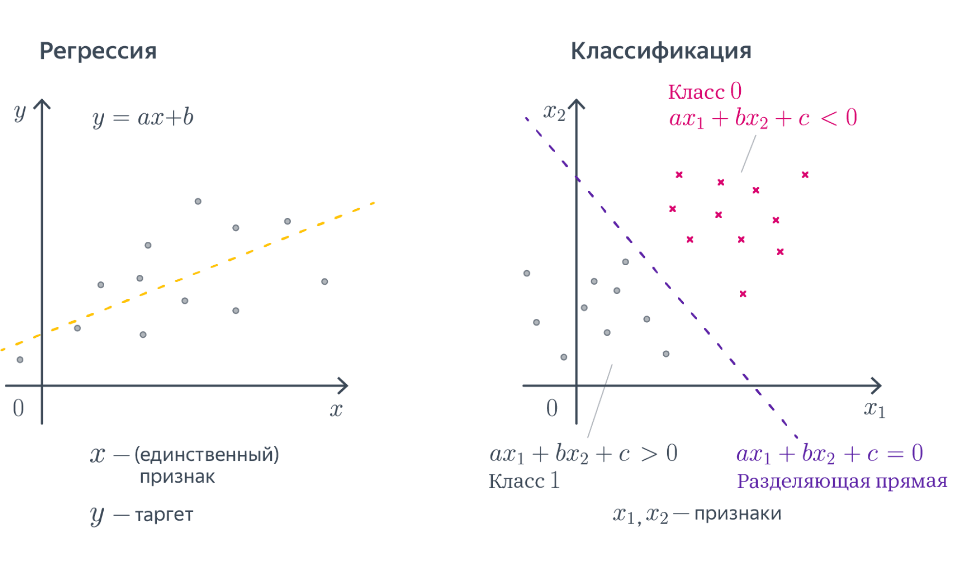
В случае более высоких размерностей вместо прямой будет гиперплоскость с аналогичным смыслом.
Вопрос на подумать. Если вы посмотрите содержание учебника, то не найдёте в нём ни «полиномиальных» моделей, ни каких-нибудь «логарифмических», хотя, казалось бы, зависимости бывают довольно сложными. Почему так?
Ответ (не открывайте сразу; сначала подумайте сами!)Линейные зависимости не так просты, как кажется. Пусть мы решаем задачу регрессии. Если мы подозреваем, что целевая переменная $y$ не выражается через $x_1, x_2$ как линейная функция, а зависит ещё от логарифма $x_1$ и ещё как-нибудь от того, разные ли знаки у признаков, то мы можем ввести дополнительные слагаемые в нашу линейную зависимость, просто объявим эти слагаемые новыми переменными и добавив перед ними соответствующие регрессионные коэффициенты
$$y approx w_1 x_1 + w_2 x_2 + w_3log{x_1} + w_4text{sgn}(x_1x_2) + w_0,$$
и в итоге из двумерной нелинейной задачи мы получили четырёхмерную линейную регрессию.
Вопрос на подумать. А как быть, если одна из фичей является категориальной, то есть принимает значения из (обычно конечного числа) значений, не являющихся числами? Например, это может быть время года, уровень образования, марка машины и так далее. Как правило, с такими значениями невозможно производить арифметические операции или же результаты их применения не имеют смысла.
Ответ (не открывайте сразу; сначала подумайте сами!)В линейную модель можно подать только численные признаки, так что категориальную фичу придётся как-то закодировать. Рассмотрим для примера вот такой датасет
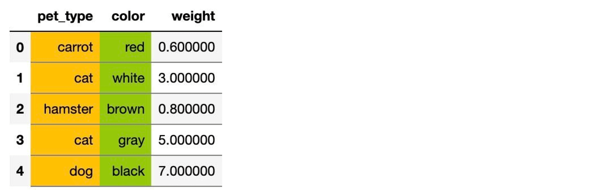
Здесь два категориальных признака – pet_type и color. Первый принимает четыре различных значения, второй – пять.
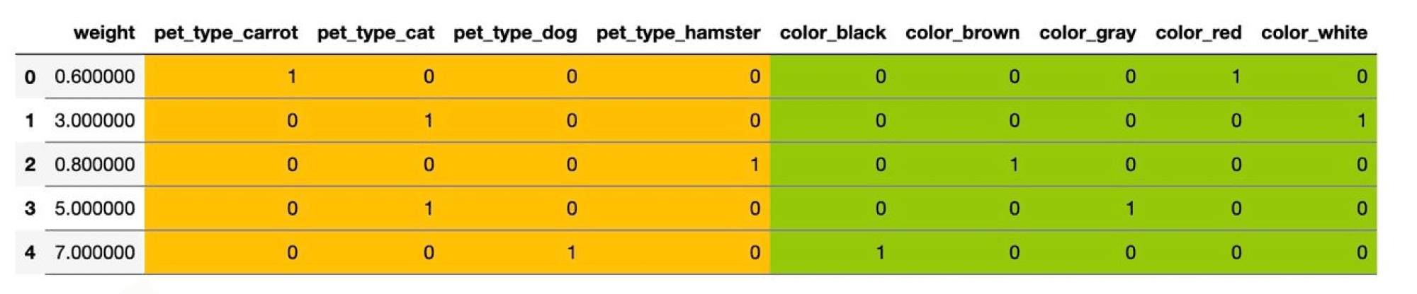
Самый простой способ – использовать one-hot кодирование (one-hot encoding). Пусть исходный признак мог принимать $M$ значений $c_1,ldots, c_M$. Давайте заменим категориальный признак на $M$ признаков, которые принимают значения $0$ и $1$: $i$-й будет отвечать на вопрос «принимает ли признак значение $c_i$?». Иными словами, вместо ячейки со значением $c_i$ у объекта появляется строка нулей и единиц, в которой единица стоит только на $i$-м месте.
В нашем примере получится вот такая табличка:
Можно было бы на этом остановиться, но добавленные признаки обладают одним неприятным свойством: в каждом из них ровно одна единица, так что сумма соответствующих столбцов равна столбцу из единиц. А это уже плохо. Представьте, что у нас есть линейная модель
$$y sim w_1x_1 + ldots + w_{D-1}x_{d-1} + w_{c_1}x_{c_1} + ldots + w_{c_M}x_{c_M} + w_0$$
Преобразуем немного правую часть:
$$ysim w_1x_1 + ldots + w_{D-1}x_{d-1} + underbrace{(w_{c_1} — w_{c_M})}_{=:w’_{c_1}}x_{c_1} + ldots + underbrace{(w_{c_{M-1}} — w_{c_M})}_{=:w’_{C_{M-1}}}x_{c_{M-1}} + w_{c_M}underbrace{(x_{c_1} + ldots + x_{c_M})}_{=1} + w_0 = $$
$$ = w_1x_1 + ldots + w_{D-1}x_{d-1} + w’_{c_1}x_{c_1} + ldots + w’_{c_{M-1}}x_{c_{M-1}} + underbrace{(w_{c_M} + w_0)}_{=w’_{0}}$$
Как видим, от одного из новых признаков можно избавиться, не меняя модель. Больше того, это стоит сделать, потому что наличие «лишних» признаков ведёт к переобучению или вовсе ломает модель – подробнее об этом мы поговорим в разделе про регуляризацию. Поэтому при использовании one-hot-encoding обычно выкидывают признак, соответствующий одному из значений. Например, в нашем примере итоговая матрица объекты-признаки будет иметь вид:

Конечно, one-hot кодирование – это самый наивный способ работы с категориальными признаками, и для более сложных фичей или фичей с большим количеством значений оно плохо подходит. С рядом более продвинутых техник вы познакомитесь в разделе про обучение представлений.
Помимо простоты, у линейных моделей есть несколько других достоинств. К примеру, мы можем достаточно легко судить, как влияют на результат те или иные признаки. Скажем, если вес $w_i$ положителен, то с ростом $i$-го признака таргет в случае регрессии будет увеличиваться, а в случае классификации наш выбор будет сдвигаться в пользу одного из классов. Значение весов тоже имеет прозрачную интерпретацию: чем вес $w_i$ больше, тем «важнее» $i$-й признак для итогового предсказания. То есть, если вы построили линейную модель, вы неплохо можете объяснить заказчику те или иные её результаты. Это качество моделей называют интерпретируемостью. Оно особенно ценится в индустриальных задачах, цена ошибки в которых высока. Если от работы вашей модели может зависеть жизнь человека, то очень важно понимать, как модель принимает те или иные решения и какими принципами руководствуется. При этом не все методы машинного обучения хорошо интерпретируемы, к примеру, поведение искусственных нейронных сетей или градиентного бустинга интерпретировать довольно сложно.
В то же время слепо доверять весам линейных моделей тоже не стоит по целому ряду причин:
- Линейные модели всё-таки довольно узкий класс функций, они неплохо работают для небольших датасетов и простых задач. Однако, если вы решаете линейной моделью более сложную задачу, то вам, скорее всего, придётся выдумывать дополнительные признаки, являющиеся сложными функциями от исходных. Поиск таких дополнительных признаков называется feature engineering, технически он устроен примерно так, как мы описали в вопросе про «полиномиальные модели». Вот только поиском таких искусственных фичей можно сильно увлечься, так что осмысленность интерпретации будет сильно зависеть от здравого смысла эксперта, строившего модель.
- Если между признаками есть приближённая линейная зависимость, коэффициенты в линейной модели могут совершенно потерять физический смысл (об этой проблеме и о том, как с ней бороться, мы поговорим дальше, когда будем обсуждать регуляризацию).
- Особенно осторожно стоит верить в утверждения вида «этот коэффициент маленький, значит, этот признак не важен». Во-первых, всё зависит от масштаба признака: вдруг коэффициент мал, чтобы скомпенсировать его. Во-вторых, зависимость действительно может быть слабой, но кто знает, в какой ситуации она окажется важна. Такие решения принимаются на основе данных, например, путём проверки статистического критерия (об этом мы коротко упомянем в разделе про вероятностные модели).
- Конкретные значения весов могут меняться в зависимости от обучающей выборки, хотя с ростом её размера они будут потихоньку сходиться к весам «наилучшей» линейной модели, которую можно было бы построить по всем-всем-всем данным на свете.
Обсудив немного общие свойства линейных моделей, перейдём к тому, как их всё-таки обучать. Сначала разберёмся с регрессией, а затем настанет черёд классификации.
Линейная регрессия и метод наименьших квадратов (МНК)
Мы начнём с использования линейных моделей для решения задачи регрессии. Простейшим примером постановки задачи линейной регрессии является метод наименьших квадратов (Ordinary least squares).
Пусть у нас задан датасет $(X, y)$, где $y=(y_i)_{i=1}^N in mathbb{R}^N$ – вектор значений целевой переменной, а $X=(x_i)_{i = 1}^N in mathbb{R}^{N times D}, x_i in mathbb{R}^D$ – матрица объекты-признаки, в которой $i$-я строка – это вектор признаков $i$-го объекта выборки. Мы хотим моделировать зависимость $y_i$ от $x_i$ как линейную функцию со свободным членом. Общий вид такой функции из $mathbb{R}^D$ в $mathbb{R}$ выглядит следующим образом:
$$color{#348FEA}{f_w(x_i) = langle w, x_i rangle + w_0}$$
Свободный член $w_0$ часто опускают, потому что такого же результата можно добиться, добавив ко всем $x_i$ признак, тождественно равный единице; тогда роль свободного члена будет играть соответствующий ему вес:
$$begin{pmatrix}x_{i1} & ldots & x_{iD} end{pmatrix}cdotbegin{pmatrix}w_1\ vdots \ w_Dend{pmatrix} + w_0 =
begin{pmatrix}1 & x_{i1} & ldots & x_{iD} end{pmatrix}cdotbegin{pmatrix}w_0 \ w_1\ vdots \ w_D end{pmatrix}$$
Поскольку это сильно упрощает запись, в дальнейшем мы будем считать, что это уже сделано и зависимость имеет вид просто $f_w(x_i) = langle w, x_i rangle$.
Сведение к задаче оптимизации
Мы хотим, чтобы на нашем датасете (то есть на парах $(x_i, y_i)$ из обучающей выборки) функция $f_w$ как можно лучше приближала нашу зависимость.

Для того, чтобы чётко сформулировать задачу, нам осталось только одно: на математическом языке выразить желание «приблизить $f_w(x)$ к $y$». Говоря простым языком, мы должны научиться измерять качество модели и минимизировать её ошибку, как-то меняя обучаемые параметры. В нашем примере обучаемые параметры — это веса $w$. Функция, оценивающая то, как часто модель ошибается, традиционно называется функцией потерь, функционалом качества или просто лоссом (loss function). Важно, чтобы её было легко оптимизировать: скажем, гладкая функция потерь – это хорошо, а кусочно постоянная – просто ужасно.
Функции потерь бывают разными. От их выбора зависит то, насколько задачу в дальнейшем легко решать, и то, в каком смысле у нас получится приблизить предсказание модели к целевым значениям. Интуитивно понятно, что для нашей текущей задачи нам нужно взять вектор $y$ и вектор предсказаний модели и как-то сравнить, насколько они похожи. Так как эти вектора «живут» в одном векторном пространстве, расстояние между ними вполне может быть функцией потерь. Более того, положительная непрерывная функция от этого расстояния тоже подойдёт в качестве функции потерь. При этом способов задать расстояние между векторами тоже довольно много. От всего этого разнообразия глаза разбегаются, но мы обязательно поговорим про это позже. Сейчас давайте в качестве лосса возьмём квадрат $L^2$-нормы вектора разницы предсказаний модели и $y$. Во-первых, как мы увидим дальше, так задачу будет нетрудно решить, а во-вторых, у этого лосса есть ещё несколько дополнительных свойств:
-
$L^2$-норма разницы – это евклидово расстояние $|y — f_w(x)|_2$ между вектором таргетов и вектором ответов модели, то есть мы их приближаем в смысле самого простого и понятного «расстояния».
-
Как мы увидим в разделе про вероятностные модели, с точки зрения статистики это соответствует гипотезе о том, что наши данные состоят из линейного «сигнала» и нормально распределенного «шума».
Так вот, наша функция потерь выглядит так:
$$L(f, X, y) = |y — f(X)|_2^2 = $$
$$= |y — Xw|_2^2 = sum_{i=1}^N(y_i — langle x_i, w rangle)^2$$
Такой функционал ошибки не очень хорош для сравнения поведения моделей на выборках разного размера. Представьте, что вы хотите понять, насколько качество модели на тестовой выборке из $2500$ объектов хуже, чем на обучающей из $5000$ объектов. Вы измерили $L^2$-норму ошибки и получили в одном случае $300$, а в другом $500$. Эти числа не очень интерпретируемы. Гораздо лучше посмотреть на среднеквадратичное отклонение
$$L(f, X, y) = frac1Nsum_{i=1}^N(y_i — langle x_i, w rangle)^2$$
По этой метрике на тестовой выборке получаем $0,12$, а на обучающей $0,1$.
Функция потерь $frac1Nsum_{i=1}^N(y_i — langle x_i, w rangle)^2$ называется Mean Squared Error, MSE или среднеквадратическим отклонением. Разница с $L^2$-нормой чисто косметическая, на алгоритм решения задачи она не влияет:
$$color{#348FEA}{text{MSE}(f, X, y) = frac{1}{N}|y — X w|_2^2}$$
В самом широком смысле, функции работают с объектами множеств: берут какой-то входящий объект из одного множества и выдают на выходе соответствующий ему объект из другого. Если мы имеем дело с отображением, которое на вход принимает функции, а на выходе выдаёт число, то такое отображение называют функционалом. Если вы посмотрите на нашу функцию потерь, то увидите, что это именно функционал. Для каждой конкретной линейной функции, которую задают веса $w_i$, мы получаем число, которое оценивает, насколько точно эта функция приближает наши значения $y$. Чем меньше это число, тем точнее наше решение, значит для того, чтобы найти лучшую модель, этот функционал нам надо минимизировать по $w$:
$$color{#348FEA}{|y — Xw|_2^2 longrightarrow min_w}$$
Эту задачу можно решать разными способами. В этой главе мы сначала решим эту задачу аналитически, а потом приближенно. Сравнение двух этих решений позволит нам проиллюстрировать преимущества того подхода, которому посвящена эта книга. На наш взгляд, это самый простой способ «на пальцах» показать суть машинного обучения.
МНК: точный аналитический метод
Точку минимума можно найти разными способами. Если вам интересно аналитическое решение, вы можете найти его в главе про матричные дифференцирования (раздел «Примеры вычисления производных сложных функций»). Здесь же мы воспользуемся геометрическим подходом.
Пусть $x^{(1)},ldots,x^{(D)}$ – столбцы матрицы $X$, то есть столбцы признаков. Тогда
$$Xw = w_1x^{(1)}+ldots+w_Dx^{(D)},$$
и задачу регрессии можно сформулировать следующим образом: найти линейную комбинацию столбцов $x^{(1)},ldots,x^{(D)}$, которая наилучшим способом приближает столбец $y$ по евклидовой норме – то есть найти проекцию вектора $y$ на подпространство, образованное векторами $x^{(1)},ldots,x^{(D)}$.
Разложим $y = y_{parallel} + y_{perp}$, где $y_{parallel} = Xw$ – та самая проекция, а $y_{perp}$ – ортогональная составляющая, то есть $y_{perp} = y — Xwperp x^{(1)},ldots,x^{(D)}$. Как это можно выразить в матричном виде? Оказывается, очень просто:
$$X^T(y — Xw) = 0$$
В самом деле, каждый элемент столбца $X^T(y — Xw)$ – это скалярное произведение строки $X^T$ (=столбца $X$ = одного из $x^{(i)}$) на $y — Xw$. Из уравнения $X^T(y — Xw) = 0$ уже очень легко выразить $w$:
$$w = (X^TX)^{-1}X^Ty$$
Вопрос на подумать Для вычисления $w_{ast}$ нам приходится обращать (квадратную) матрицу $X^TX$, что возможно, только если она невырожденна. Что это значит с точки зрения анализа данных? Почему мы верим, что это выполняется во всех разумных ситуациях?
Ответ (не открывайте сразу; сначала подумайте сами!)Как известно из линейной алгебры, для вещественной матрицы $X$ ранги матриц $X$ и $X^TX$ совпадают. Матрица $X^TX$ невырожденна тогда и только тогда, когда её ранг равен числу её столбцов, что равно числу столбцов матрицы $X$. Иными словами, формула регрессии поломается, только если столбцы матрицы $X$ линейно зависимы. Столбцы матрицы $X$ – это признаки. А если наши признаки линейно зависимы, то, наверное, что-то идёт не так и мы должны выкинуть часть из них, чтобы остались только линейно независимые.
Другое дело, что зачастую признаки могут быть приближённо линейно зависимы, особенно если их много. Тогда матрица $X^TX$ будет близка к вырожденной, и это, как мы дальше увидим, будет вести к разным, в том числе вычислительным проблемам.
Вычислительная сложность аналитического решения — $O(N^2D + D^3)$, где $N$ — длина выборки, $D$ — число признаков у одного объекта. Слагаемое $N^2D$ отвечает за сложность перемножения матриц $X^T$ и $X$, а слагаемое $D^3$ — за сложность обращения их произведения. Перемножать матрицы $(X^TX)^{-1}$ и $X^T$ не стоит. Гораздо лучше сначала умножить $y$ на $X^T$, а затем полученный вектор на $(X^TX)^{-1}$: так будет быстрее и, кроме того, не нужно будет хранить матрицу $(X^TX)^{-1}X^T$.
Вычисление можно ускорить, используя продвинутые алгоритмы перемножения матриц или итерационные методы поиска обратной матрицы.
Проблемы «точного» решения
Заметим, что для получения ответа нам нужно обратить матрицу $X^TX$. Это создает множество проблем:
- Основная проблема в обращении матрицы — это то, что вычислительно обращать большие матрицы дело сложное, а мы бы хотели работать с датасетами, в которых у нас могут быть миллионы точек,
- Матрица $X^TX$, хотя почти всегда обратима в разумных задачах машинного обучения, зачастую плохо обусловлена. Особенно если признаков много, между ними может появляться приближённая линейная зависимость, которую мы можем упустить на этапе формулировки задачи. В подобных случаях погрешность нахождения $w$ будет зависеть от квадрата числа обусловленности матрицы $X$, что очень плохо. Это делает полученное таким образом решение численно неустойчивым: малые возмущения $y$ могут приводить к катастрофическим изменениям $w$.
Пара слов про число обусловленности.Пожертвовав математической строгостью, мы можем считать, что число обусловленности матрицы $X$ – это корень из отношения наибольшего и наименьшего из собственных чисел матрицы $X^TX$. Грубо говоря, оно показывает, насколько разного масштаба бывают собственные значения $X^TX$. Если рассмотреть $L^2$-норму ошибки предсказания, как функцию от $w$, то её линии уровня будут эллипсоидами, форма которых определяется квадратичной формой с матрицей $X^TX$ (проверьте это!). Таким образом, число обусловленности говорит о том, насколько вытянутыми являются эти эллипсоиды.ПодробнееДанные проблемы не являются поводом выбросить решение на помойку. Существует как минимум два способа улучшить его численные свойства, однако если вы не знаете про сингулярное разложение, то лучше вернитесь сюда, когда узнаете.
-
Построим $QR$-разложение матрицы $X$. Напомним, что это разложение, в котором матрица $Q$ ортогональна по столбцам (то есть её столбцы ортогональны и имеют длину 1; в частности, $Q^TQ=E$), а $R$ квадратная и верхнетреугольная. Подставив его в формулу, получим
$$w = ((QR)^TQR)^{-1}(QR)^T y = (R^Tunderbrace{Q^TQ}_{=E}R)^{-1}R^TQ^Ty = R^{-1}R^{-T}R^TQ^Ty = R^{-1}Q^Ty$$
Отметим, что написать $(R^TR)^{-1} = R^{-1}R^{-T}$ мы имеем право благодаря тому, что $R$ квадратная. Полученная формула намного проще, обращение верхнетреугольной матрицы (=решение системы с верхнетреугольной левой частью) производится быстро и хорошо, погрешность вычисления $w$ будет зависеть просто от числа обусловленности матрицы $X$, а поскольку нахождение $QR$-разложения является достаточно стабильной операцией, мы получаем решение с более хорошими, чем у исходной формулы, численными свойствами.
-
Также можно использовать псевдообратную матрицу, построенную с помощью сингулярного разложения, о котором подробно написано в разделе про матричные разложения. А именно, пусть
$$A = Uunderbrace{mathrm{diag}(sigma_1,ldots,sigma_r)}_{=Sigma}V^T$$
– это усечённое сингулярное разложение, где $r$ – это ранг $A$. В таком случае диагональная матрица посередине является квадратной, $U$ и $V$ ортогональны по столбцам: $U^TU = E$, $V^TV = E$. Тогда
$$w = (VSigma underbrace{U^TU}_{=E}Sigma V^T)^{-1}VSigma U^Ty$$
Заметим, что $VSigma^{-2}V^Tcdot VSigma^2V^T = E = VSigma^2V^Tcdot VSigma^{-2}V^T$, так что $(VSigma^2 V^T)^{-1} = VSigma^{-2}V^T$, откуда
$$w = VSigma^{-2}underbrace{V^TV}_{=E}V^Tcdot VSigma U^Ty = VSigma^{-1}Uy$$
Хорошие численные свойства сингулярного разложения позволяют утверждать, что и это решение ведёт себя довольно неплохо.
Тем не менее, вычисление всё равно остаётся довольно долгим и будет по-прежнему страдать (хоть и не так сильно) в случае плохой обусловленности матрицы $X$.
Полностью вылечить проблемы мы не сможем, но никто и не обязывает нас останавливаться на «точном» решении (которое всё равно никогда не будет вполне точным). Поэтому ниже мы познакомим вас с совершенно другим методом.
МНК: приближенный численный метод
Минимизируемый функционал является гладким и выпуклым, а это значит, что можно эффективно искать точку его минимума с помощью итеративных градиентных методов. Более подробно вы можете прочитать о них в разделе про методы оптимизации, а здесь мы лишь коротко расскажем об одном самом базовом подходе.
Как известно, градиент функции в точке направлен в сторону её наискорейшего роста, а антиградиент (противоположный градиенту вектор) в сторону наискорейшего убывания. То есть имея какое-то приближение оптимального значения параметра $w$, мы можем его улучшить, посчитав градиент функции потерь в точке и немного сдвинув вектор весов в направлении антиградиента:
$$w_j mapsto w_j — alpha frac{d}{d{w_j}} L(f_w, X, y) $$
где $alpha$ – это параметр алгоритма («темп обучения»), который контролирует величину шага в направлении антиградиента. Описанный алгоритм называется градиентным спуском.
Посмотрим, как будет выглядеть градиентный спуск для функции потерь $L(f_w, X, y) = frac1Nvertvert Xw — yvertvert^2$. Градиент квадрата евклидовой нормы мы уже считали; соответственно,
$$
nabla_wL = frac2{N} X^T (Xw — y)
$$
Следовательно, стартовав из какого-то начального приближения, мы можем итеративно уменьшать значение функции, пока не сойдёмся (по крайней мере в теории) к минимуму (вообще говоря, локальному, но в данном случае глобальному).
Алгоритм градиентного спуска
w = random_normal()             # можно пробовать и другие виды инициализации
repeat S times:                 # другой вариант: while abs(err) > tolerance
   f = X.dot(w)                 # посчитать предсказание
   err = f - y                  # посчитать ошибку
   grad = 2 * X.T.dot(err) / N  # посчитать градиент
   w -= alpha * grad            # обновить веса
С теоретическими результатами о скорости и гарантиях сходимости градиентного спуска вы можете познакомиться в главе про методы оптимизации. Мы позволим себе лишь несколько общих замечаний:
- Поскольку задача выпуклая, выбор начальной точки влияет на скорость сходимости, но не настолько сильно, чтобы на практике нельзя было стартовать всегда из нуля или из любой другой приятной вам точки;
- Число обусловленности матрицы $X$ существенно влияет на скорость сходимости градиентного спуска: чем более вытянуты эллипсоиды уровня функции потерь, тем хуже;
- Темп обучения $alpha$ тоже сильно влияет на поведение градиентного спуска; вообще говоря, он является гиперпараметром алгоритма, и его, возможно, придётся подбирать отдельно. Другими гиперпараметрами являются максимальное число итераций $S$ и/или порог tolerance.
Иллюстрация.Рассмотрим три задачи регрессии, для которых матрица $X$ имеет соответственно маленькое, среднее и большое числа обусловленности. Будем строить для них модели вида $y=w_1x_1 + w_2x_2$. Раскрасим плоскость $(w_1, w_2)$ в соответствии со значениями $|X_{text{train}}w — y_{text{train}}|^2$. Тёмная область содержит минимум этой функции – оптимальное значение $w_{ast}$. Также запустим из из двух точек градиентный спуск с разными значениями темпа обучения $alpha$ и посмотрим, что получится:
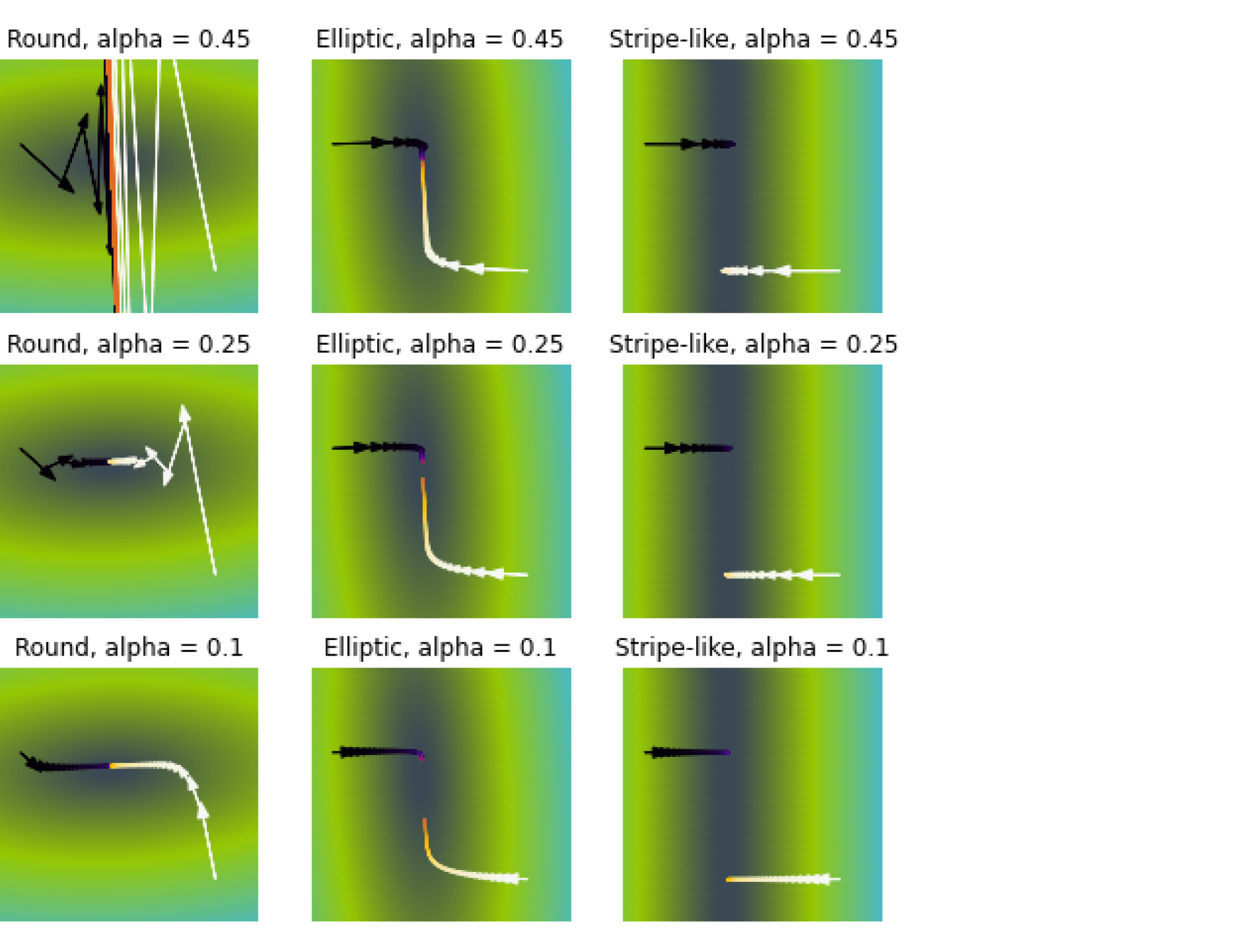 Заголовки графиков («Round», «Elliptic», «Stripe-like») относятся к форме линий уровня потерь (чем более они вытянуты, тем хуже обусловлена задача и тем хуже может вести себя градиентный спуск).
Итог: при неудачном выборе $alpha$ алгоритм не сходится или идёт вразнос, а для плохо обусловленной задачи он сходится абы куда.
Вычислительная сложность градиентного спуска – $O(NDS)$, где, как и выше, $N$ – длина выборки, $D$ – число признаков у одного объекта. Сравните с оценкой $O(N^2D + D^3)$ для «наивного» вычисления аналитического решения.
Сложность по памяти – $O(ND)$ на хранение выборки. В памяти мы держим и выборку, и градиент, но в большинстве реалистичных сценариев доминирует выборка.
Стохастический градиентный спуск
На каждом шаге градиентного спуска нам требуется выполнить потенциально дорогую операцию вычисления градиента по всей выборке (сложность $O(ND)$). Возникает идея заменить градиент его оценкой на подвыборке (в английской литературе такую подвыборку обычно именуют batch или mini-batch; в русской разговорной терминологии тоже часто встречается слово батч или мини-батч).
А именно, если функция потерь имеет вид суммы по отдельным парам объект-таргет
$$L(w, X, y) = frac1Nsum_{i=1}^NL(w, x_i, y_i),$$
а градиент, соответственно, записывается в виде
$$nabla_wL(w, X, y) = frac1Nsum_{i=1}^Nnabla_wL(w, x_i, y_i),$$
то предлагается брать оценку
$$nabla_wL(w, X, y) approx frac1Bsum_{t=1}^Bnabla_wL(w, x_{i_t}, y_{i_t})$$
для некоторого подмножества этих пар $(x_{i_t}, y_{i_t})_{t=1}^B$. Обратите внимание на множители $frac1N$ и $frac1B$ перед суммами. Почему они нужны? Полный градиент $nabla_wL(w, X, y)$ можно воспринимать как среднее градиентов по всем объектам, то есть как оценку матожидания $mathbb{E}nabla_wL(w, x, y)$; тогда, конечно, оценка матожидания по меньшей подвыборке тоже будет иметь вид среднего градиентов по объектам этой подвыборки.
Как делить выборку на батчи? Ясно, что можно было бы случайным образом сэмплировать их из полного датасета, но даже если использовать быстрый алгоритм вроде резервуарного сэмплирования, сложность этой операции не самая оптимальная. Поэтому используют линейный проход по выборке (которую перед этим лучше всё-таки случайным образом перемешать). Давайте введём ещё один параметр нашего алгоритма: размер батча, который мы обозначим $B$. Теперь на $B$ очередных примерах вычислим градиент и обновим веса модели. При этом вместо количества шагов алгоритма обычно задают количество эпох $E$. Это ещё один гиперпараметр. Одна эпоха – это один полный проход нашего сэмплера по выборке. Заметим, что если выборка очень большая, а модель компактная, то даже первый проход бывает можно не заканчивать.
Алгоритм:
 w = normal(0, 1)
 repeat E times:
   for i = B, i <= n, i += B
      X_batch = X[i-B : i]
      y_batch = y[i-B : i]
      f = X_batch.dot(w)                 # посчитать предсказание
      err = f - y_batch                  # посчитать ошибку
      grad = 2 * X_batch.T.dot(err) / B  # посчитать градиент
      w -= alpha * grad
Сложность по времени – $O(NDE)$. На первый взгляд, она такая же, как и у обычного градиентного спуска, но заметим, что мы сделали в $N / B$ раз больше шагов, то есть веса модели претерпели намного больше обновлений.
Сложность по памяти можно довести до $O(BD)$: ведь теперь всю выборку не надо держать в памяти, а достаточно загружать лишь текущий батч (а остальная выборка может лежать на диске, что удобно, так как в реальности задачи, в которых выборка целиком не влезает в оперативную память, встречаются сплошь и рядом). Заметим, впрочем, что при этом лучше бы $B$ взять побольше: ведь чтение с диска – намного более затратная по времени операция, чем чтение из оперативной памяти.
В целом, разницу между алгоритмами можно представлять как-то так: 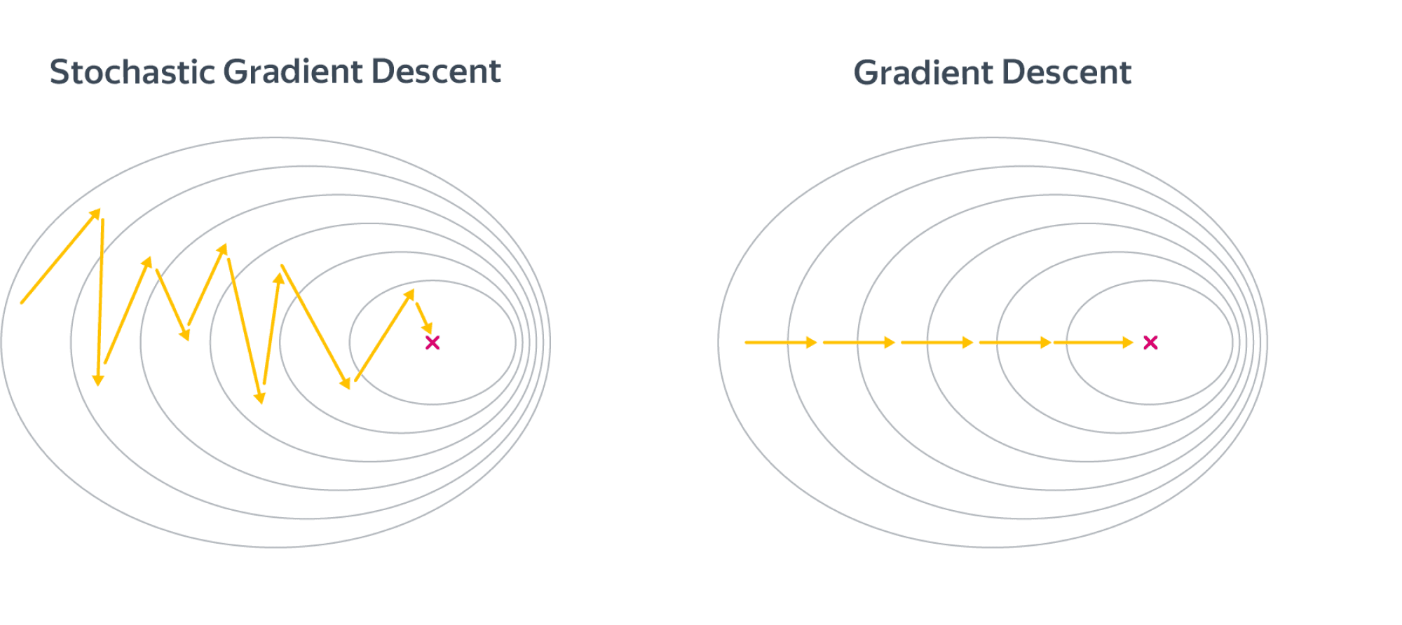
Шаги стохастического градиентного спуска заметно более шумные, но считать их получается значительно быстрее. В итоге они тоже сходятся к оптимальному значению из-за того, что матожидание оценки градиента на батче равно самому градиенту. По крайней мере, сходимость можно получить при хорошо подобранных коэффициентах темпа обучения в случае выпуклого функционала качества. Подробнее мы об этом поговорим в главе про оптимизацию. Для сложных моделей и лоссов стохастический градиентный спуск может сходиться плохо или застревать в локальных минимумах, поэтому придумано множество его улучшений. О некоторых из них также рассказано в главе про оптимизацию.
Существует определённая терминологическая путаница, иногда стохастическим градиентным спуском называют версию алгоритма, в которой размер батча равен единице (то есть максимально шумная и быстрая версия алгоритма), а версии с бОльшим размером батча называют batch gradient descent. В книгах, которые, возможно, старше вас, такая процедура иногда ещё называется incremental gradient descent. Это не очень принципиально, но вы будьте готовы, если что.
Вопрос на подумать. Вообще говоря, если объём данных не слишком велик и позволяет это сделать, объекты лучше случайным образом перемешивать перед тем, как подавать их в алгоритм стохастического градиентного спуска. Как вам кажется, почему?
Также можно использовать различные стратегии отбора объектов. Например, чаще брать объекты, на которых ошибка больше. Какие ещё стратегии вы могли бы придумать?
Ответ (не открывайте сразу; сначала подумайте сами!)Легко представить себе ситуацию, в которой объекты как-нибудь неудачно упорядочены, скажем, по возрастанию таргета. Тогда модель будет попеременно то запоминать, что все таргеты маленькие, то – что все таргеты большие. Это может и не повлиять на качество итоговой модели, но может привести и к довольно печальным последствиям. И вообще, чем более разнообразные батчи модель увидит в процессе обучения, тем лучше.
Стратегий можно придумать много. Например, не брать объекты, на которых ошибка слишком большая (возможно, это выбросы – зачем на них учиться), или вообще не брать те, на которых ошибка достаточно мала (они «ничему не учат»). Рекомендуем, впрочем, прибегать к этим эвристикам, только если вы понимаете, зачем они вам нужны и почему есть надежда, что они помогут.
Неградиентные методы
После прочтения этой главы у вас может сложиться ощущение, что приближённые способы решения ML задач и градиентные методы – это одно и тоже, но вы будете правы в этом только на 98%. В принципе, существуют и другие способы численно решать эти задачи, но в общем случае они работают гораздо хуже, чем градиентный спуск, и не обладают таким хорошим теоретическим обоснованием. Мы не будем рассказывать про них подробно, но можете на досуге почитать, скажем, про Stepwise regression, Orthogonal matching pursuit или LARS. У LARS, кстати, есть довольно интересное свойство: он может эффективно работать на выборках, в которых число признаков больше числа примеров. С алгоритмом LARS вы можете познакомиться в главе про оптимизацию.
Регуляризация
Всегда ли решение задачи регрессии единственно? Вообще говоря, нет. Так, если в выборке два признака будут линейно зависимы (и следовательно, ранг матрицы будет меньше $D$), то гарантировано найдётся такой вектор весов $nu$ что $langlenu, x_irangle = 0 forall x_i$. В этом случае, если какой-то $w$ является решением оптимизационной задачи, то и $w + alpha nu $ тоже является решением для любого $alpha$. То есть решение не только не обязано быть уникальным, так ещё может быть сколь угодно большим по модулю. Это создаёт вычислительные трудности. Малые погрешности признаков сильно возрастают при предсказании ответа, а в градиентном спуске накапливается погрешность из-за операций со слишком большими числами.
Конечно, в жизни редко бывает так, что признаки строго линейно зависимы, а вот быть приближённо линейно зависимыми они вполне могут быть. Такая ситуация называется мультиколлинеарностью. В этом случае у нас, всё равно, возникают проблемы, близкие к описанным выше. Дело в том, что $Xnusim 0$ для вектора $nu$, состоящего из коэффициентов приближённой линейной зависимости, и, соответственно, $X^TXnuapprox 0$, то есть матрица $X^TX$ снова будет близка к вырожденной. Как и любая симметричная матрица, она диагонализуется в некотором ортонормированном базисе, и некоторые из собственных значений $lambda_i$ близки к нулю. Если вектор $X^Ty$ в выражении $(X^TX)^{-1}X^Ty$ будет близким к соответствующему собственному вектору, то он будет умножаться на $1 /{lambda_i}$, что опять же приведёт к появлению у $w$ очень больших по модулю компонент (при этом $w$ ещё и будет вычислен с большой погрешностью из-за деления на маленькое число). И, конечно же, все ошибки и весь шум, которые имелись в матрице $X$, при вычислении $ysim Xw$ будут умножаться на эти большие и неточные числа и возрастать во много-много раз, что приведёт к проблемам, от которых нас не спасёт никакое сингулярное разложение.
Важно ещё отметить, что в случае, когда несколько признаков линейно зависимы, веса $w_i$ при них теряют физический смысл. Может даже оказаться, что вес признака, с ростом которого таргет, казалось бы, должен увеличиваться, станет отрицательным. Это делает модель не только неточной, но и принципиально не интерпретируемой. Вообще, неадекватность знаков или величины весов – хорошее указание на мультиколлинеарность.
Для того, чтобы справиться с этой проблемой, задачу обычно регуляризуют, то есть добавляют к ней дополнительное ограничение на вектор весов. Это ограничение можно, как и исходный лосс, задавать по-разному, но, как правило, ничего сложнее, чем $L^1$- и $L^2$-нормы, не требуется.
Вместо исходной задачи теперь предлагается решить такую:
$$color{#348FEA}{min_w L(f, X, y) = min_w(|X w — y|_2^2 + lambda |w|^k_k )}$$
$lambda$ – это очередной параметр, а $|w|^k_k $ – это один из двух вариантов:
$$color{#348FEA}{|w|^2_2 = w^2_1 + ldots + w^2_D}$$
или
$$color{#348FEA}{|w|_1^1 = vert w_1 vert + ldots + vert w_D vert}$$
Добавка $lambda|w|^k_k$ называется регуляризационным членом или регуляризатором, а число $lambda$ – коэффициентом регуляризации.
Коэффициент $lambda$ является гиперпараметром модели и достаточно сильно влияет на качество итогового решения. Его подбирают по логарифмической шкале (скажем, от 1e-2 до 1e+2), используя для сравнения моделей с разными значениями $lambda$ дополнительную валидационную выборку. При этом качество модели с подобранным коэффициентом регуляризации уже проверяют на тестовой выборке, чтобы исключить переобучение. Более подробно о том, как нужно подбирать гиперпараметры, вы можете почитать в соответствующей главе.
Отдельно надо договориться о том, что вес $w_0$, соответствующий отступу от начала координат (то есть признаку из всех единичек), мы регуляризовать не будем, потому что это не имеет смысла: если даже все значения $y$ равномерно велики, это не должно портить качество обучения. Обычно это не отображают в формулах, но если придираться к деталям, то стоило бы написать сумму по всем весам, кроме $w_0$:
$$|w|^2_2 = sum_{color{red}{j=1}}^{D}w_j^2,$$
$$|w|_1 = sum_{color{red}{j=1}}^{D} vert w_j vert$$
В случае $L^2$-регуляризации решение задачи изменяется не очень сильно. Например, продифференцировав новый лосс по $w$, легко получить, что «точное» решение имеет вид:
$$w = (X^TX + lambda I)^{-1}X^Ty$$
Отметим, что за этой формулой стоит и понятная численная интуиция: раз матрица $X^TX$ близка к вырожденной, то обращать её сродни самоубийству. Мы лучше слегка исказим её добавкой $lambda I$, которая увеличит все собственные значения на $lambda$, отодвинув их от нуля. Да, аналитическое решение перестаёт быть «точным», но за счёт снижения численных проблем мы получим более качественное решение, чем при использовании «точной» формулы.
В свою очередь, градиент функции потерь
$$L(f_w, X, y) = |Xw — y|^2 + lambda|w|^2$$
по весам теперь выглядит так:
$$
nabla_wL(f_w, X, y) = 2X^T(Xw — y) + 2lambda w
$$
Подставив этот градиент в алгоритм стохастического градиентного спуска, мы получаем обновлённую версию приближенного алгоритма, отличающуюся от старой только наличием дополнительного слагаемого.
Вопрос на подумать. Рассмотрим стохастический градиентный спуск для $L^2$-регуляризованной линейной регрессии с батчами размера $1$. Выберите правильный вариант шага SGD:
(а) $w_imapsto w_i — 2alpha(langle w, x_jrangle — y_j)x_{ji} — frac{2alphalambda}N w_i,quad i=1,ldots,D$;
(б) $w_imapsto w_i — 2alpha(langle w, x_jrangle — y_j)x_{ji} — 2alphalambda w_i,quad i=1,ldots,D$;
(в) $w_imapsto w_i — 2alpha(langle w, x_jrangle — y_j)x_{ji} — 2lambda N w_i,quad i=1,ldots D$.
Ответ (не открывайте сразу; сначала подумайте сами!)Не регуляризованная функция потерь имеет вид $mathcal{L}(X, y, w) = frac1Nsum_{i=1}^Nmathcal{L}(x_i, y_i, w)$, и её можно воспринимать, как оценку по выборке $(x_i, y_i)_{i=1}^N$ идеальной функции потерь
$$mathcal{L}(w) = mathbb{E}_{x, y}mathcal{L}(x, y, w)$$
Регуляризационный член не зависит от выборки и добавляется отдельно:
$$mathcal{L}_{text{reg}}(w) = mathbb{E}_{x, y}mathcal{L}(x, y, w) + lambda|w|^2$$
Соответственно, идеальный градиент регуляризованной функции потерь имеет вид
$$nabla_wmathcal{L}_{text{reg}}(w) = mathbb{E}_{x, y}nabla_wmathcal{L}(x, y, w) + 2lambda w,$$
Градиент по батчу – это тоже оценка градиента идеальной функции потерь, только не на выборке $(X, y)$, а на батче $(x_{t_i}, y_{t_i})_{i=1}^B$ размера $B$. Он будет выглядеть так:
$$nabla_wmathcal{L}_{text{reg}}(w) = frac1Bsum_{i=1}^Bnabla_wmathcal{L}(x_{t_i}, y_{t_i}, w) + 2lambda w.$$
Как видите, коэффициентов, связанных с числом объектов в батче или в исходной выборке, во втором слагаемом нет. Так что верным является второй вариант. Кстати, обратите внимание, что в третьем ещё и нет коэффициента $alpha$ перед производной регуляризационного слагаемого, это тоже ошибка.
Вопрос на подумать. Распишите процедуру стохастического градиентного спуска для $L^1$-регуляризованной линейной регрессии. Как вам кажется, почему никого не волнует, что функция потерь, строго говоря, не дифференцируема?
Ответ (не открывайте сразу; сначала подумайте сами!)Распишем для случая батча размера 1:
$$w_imapsto w_i — alpha(langle w, x_jrangle — y_j)x_{ji} — frac{lambda}Ncdot text{sign}(w_i),quad i=1,ldots,D$$
Функция потерь не дифференцируема лишь в одной точке. Так как в машинном обучении чаще всего мы имеем дело с данными вероятностного характера, это не влечёт каких-то особых проблем. Дело в том, что попадание прямо в ноль очень маловероятно из-за численных погрешностей в данных, так что мы можем просто доопределить производную в одной точке, а если даже пару раз попадём в неё за время обучения, это не приведёт к каким-то значительным изменениям результатов.
Отметим, что $L^1$- и $L^2$-регуляризацию можно определять для любой функции потерь $L(w, X, y)$ (и не только в задаче регрессии, а и, например, в задаче классификации тоже). Новая функция потерь будет соответственно равна
$$widetilde{L}(w, X, y) = L(w, X, y) + lambda|w|_1$$
или
$$widetilde{L}(w, X, y) = L(w, X, y) + lambda|w|_2^2$$
Разреживание весов в $L^1$-регуляризации
$L^2$-регуляризация работает прекрасно и используется в большинстве случаев, но есть одна полезная особенность $L^1$-регуляризации: её применение приводит к тому, что у признаков, которые не оказывают большого влияния на ответ, вес в результате оптимизации получается равным $0$. Это позволяет удобным образом удалять признаки, слабо влияющие на таргет. Кроме того, это даёт возможность автоматически избавляться от признаков, которые участвуют в соотношениях приближённой линейной зависимости, соответственно, спасает от проблем, связанных с мультиколлинеарностью, о которых мы писали выше.
Не очень строгим, но довольно интуитивным образом это можно объяснить так:
- В точке оптимума линии уровня регуляризационного члена касаются линий уровня основного лосса, потому что, во-первых, и те, и другие выпуклые, а во-вторых, если они пересекаются трансверсально, то существует более оптимальная точка:
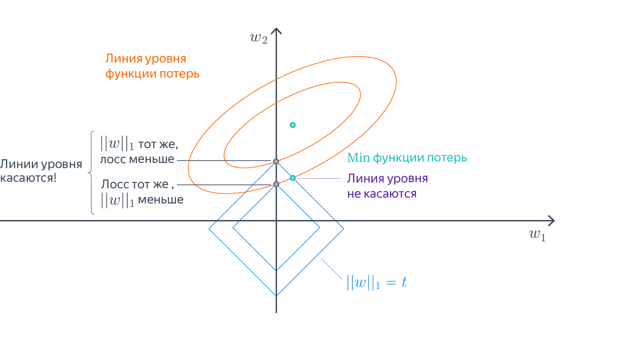
- Линии уровня $L^1$-нормы – это $N$-мерные октаэдры. Точки их касания с линиями уровня лосса, скорее всего, лежат на грани размерности, меньшей $N-1$, то есть как раз в области, где часть координат равна нулю:
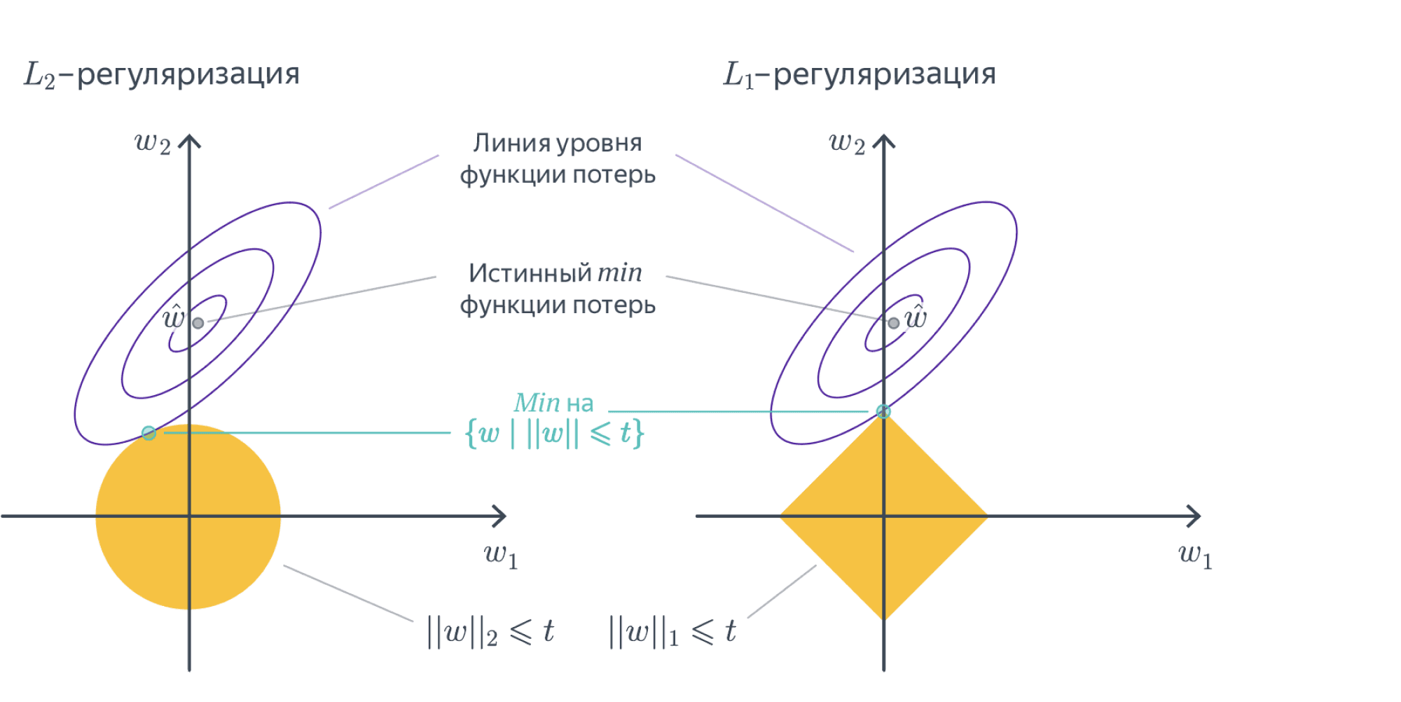
Заметим, что данное построение говорит о том, как выглядит оптимальное решение задачи, но ничего не говорит о способе, которым это решение можно найти. На самом деле, найти такой оптимум непросто: у $L^1$ меры довольно плохая производная. Однако, способы есть. Можете на досуге прочитать, например, вот эту статью о том, как работало предсказание CTR в google в 2012 году. Там этой теме посвящается довольно много места. Кроме того, рекомендуем посмотреть про проксимальные методы в разделе этой книги про оптимизацию в ML.
Заметим также, что вообще-то оптимизация любой нормы $L_x, 0 < x leq 1$, приведёт к появлению разреженных векторов весов, просто если c $L^1$ ещё хоть как-то можно работать, то с остальными всё будет ещё сложнее.
Другие лоссы
Стохастический градиентный спуск можно очевидным образом обобщить для решения задачи линейной регрессии с любой другой функцией потерь, не только квадратичной: ведь всё, что нам нужно от неё, – это чтобы у функции потерь был градиент. На практике это делают редко, но тем не менее рассмотрим ещё пару вариантов.
MAE
Mean absolute error, абсолютная ошибка, появляется при замене $L^2$ нормы в MSE на $L^1$:
$$color{#348FEA}{MAE(y, widehat{y}) = frac1Nsum_{i=1}^N vert y_i — widehat{y}_ivert}$$
Можно заметить, что в MAE по сравнению с MSE существенно меньший вклад в ошибку будут вносить примеры, сильно удалённые от ответов модели. Дело тут в том, что в MAE мы считаем модуль расстояния, а не квадрат, соответственно, вклад больших ошибок в MSE получается существенно больше. Такая функция потерь уместна в случаях, когда вы пытаетесь обучить регрессию на данных с большим количеством выбросов в таргете.
Иначе на эту разницу можно посмотреть так: MSE приближает матожидание условного распределения $y mid x$, а MAE – медиану.
MAPE
Mean absolute percentage error, относительная ошибка.
$$MAPE(y, widehat{y}) = frac1Nsum_{i=1}^N left|frac{widehat{y}_i-y_i}{y_i}right|$$
Часто используется в задачах прогнозирования (например, погоды, загруженности дорог, кассовых сборов фильмов, цен), когда ответы могут быть различными по порядку величины, и при этом мы бы хотели верно угадать порядок, то есть мы не хотим штрафовать модель за предсказание 2000 вместо 1000 в разы сильней, чем за предсказание 2 вместо 1.
Вопрос на подумать. Кроме описанных выше в задаче линейной регрессии можно использовать и другие функции потерь, например, Huber loss:
$$mathcal{L}(f, X, y) = sum_{i=1}^Nh_{delta}(y_i — langle w_i, xrangle),mbox{ где }h_{delta}(z) = begin{cases}
frac12z^2, |z|leqslantdelta,\
delta(|z| — frac12delta), |z| > delta
end{cases}$$
Число $delta$ является гиперпараметром. Сложная формула при $vert zvert > delta$ нужна, чтобы функция $h_{delta}(z)$ была непрерывной. Попробуйте объяснить, зачем может быть нужна такая функция потерь.
Ответ (не открывайте сразу; сначала подумайте сами!)Часто требования формулируют в духе «функция потерь должна слабее штрафовать то-то и сильней штрафовать вот это». Например, $L^2$-регуляризованный лосс штрафует за большие по модулю веса. В данном случае можно заметить, что при небольших значениях ошибки берётся просто MSE, а при больших мы начинаем штрафовать нашу модель менее сурово. Например, это может быть полезно для того, чтобы выбросы не так сильно влияли на результат обучения.
Линейная классификация
Теперь давайте поговорим про задачу классификации. Для начала будем говорить про бинарную классификацию на два класса. Обобщить эту задачу до задачи классификации на $K$ классов не составит большого труда. Пусть теперь наши таргеты $y$ кодируют принадлежность к положительному или отрицательному классу, то есть принадлежность множеству ${-1,1}$ (в этой главе договоримся именно так обозначать классы, хотя в жизни вам будут нередко встречаться и метки ${0,1}$), а $x$ – по-прежнему векторы из $mathbb{R}^D$. Мы хотим обучить линейную модель так, чтобы плоскость, которую она задаёт, как можно лучше отделяла объекты одного класса от другого.
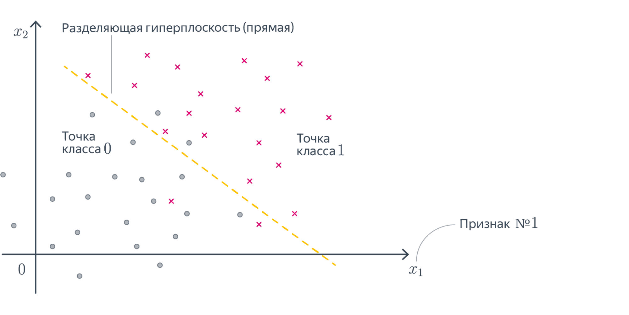
В идеальной ситуации найдётся плоскость, которая разделит классы: положительный окажется с одной стороны от неё, а отрицательный с другой. Выборка, для которой это возможно, называется линейно разделимой. Увы, в реальной жизни такое встречается крайне редко.
Как обучить линейную модель классификации, нам ещё предстоит понять, но уже ясно, что итоговое предсказание можно будет вычислить по формуле
$$y = text{sign} langle w, x_irangle$$
Почему бы не решать, как задачу регрессии?Мы можем попробовать предсказывать числа $-1$ и $1$, минимизируя для этого, например, MSE с последующим взятием знака, но ничего хорошего не получится. Во-первых, регрессия почти не штрафует за ошибки на объектах, которые лежат близко к *разделяющей плоскости*, но не с той стороны. Во вторых, ошибкой будет считаться предсказание, например, $5$ вместо $1$, хотя нам-то на самом деле не важно, какой у числа модуль, лишь бы знак был правильным. Если визуализировать такое решение, то проблемы тоже вполне заметны:
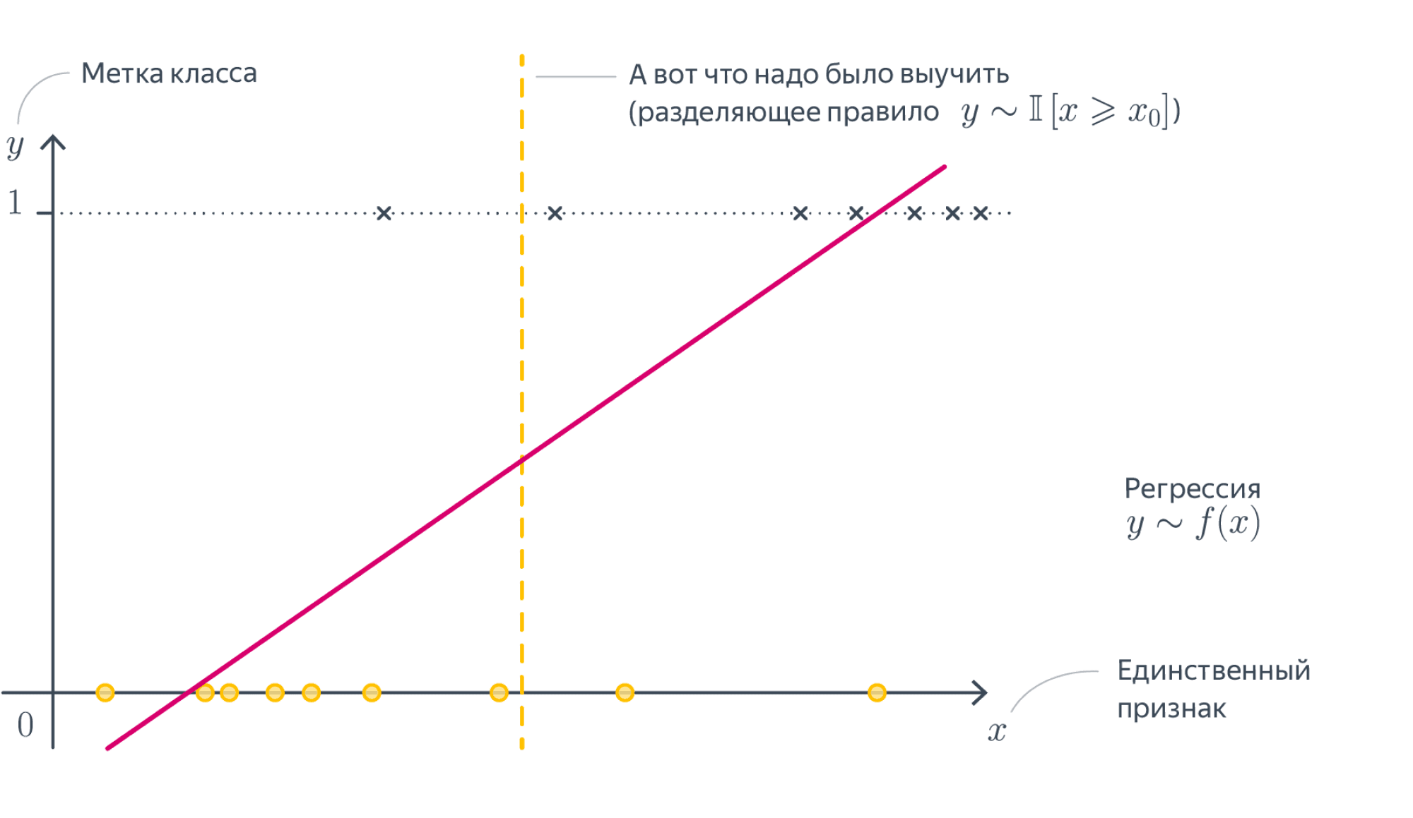
Нам нужна прямая, которая разделяет эти точки, а не проходит через них!
Сконструируем теперь функционал ошибки так, чтобы он вышеперечисленными проблемами не обладал. Мы хотим минимизировать число ошибок классификатора, то есть
$$sum_i mathbb{I}[y_i neq sign langle w, x_irangle]longrightarrow min_w$$
Домножим обе части на $$y_i$$ и немного упростим
$$sum_i mathbb{I}[y_i langle w, x_irangle < 0]longrightarrow min_w$$
Величина $M = y_i langle w, x_irangle$ называется отступом (margin) классификатора. Такая фунция потерь называется misclassification loss. Легко видеть, что
-
отступ положителен, когда $sign(y_i) = sign(langle w, x_irangle)$, то есть класс угадан верно; при этом чем больше отступ, тем больше расстояние от $x_i$ до разделяющей гиперплоскости, то есть «уверенность классификатора»;
-
отступ отрицателен, когда $sign(y_i) ne sign(langle w, x_irangle)$, то есть класс угадан неверно; при этом чем больше по модулю отступ, тем более сокрушительно ошибается классификатор.
От каждого из отступов мы вычисляем функцию
$$F(M) = mathbb{I}[M < 0] = begin{cases}1, M < 0,\ 0, Mgeqslant 0end{cases}$$
Она кусочно-постоянная, и из-за этого всю сумму невозможно оптимизировать градиентными методами: ведь её производная равна нулю во всех точках, где она существует. Но мы можем мажорировать её какой-нибудь более гладкой функцией, и тогда задачу можно будет решить. Функции можно использовать разные, у них свои достоинства и недостатки, давайте рассмотрим несколько примеров:
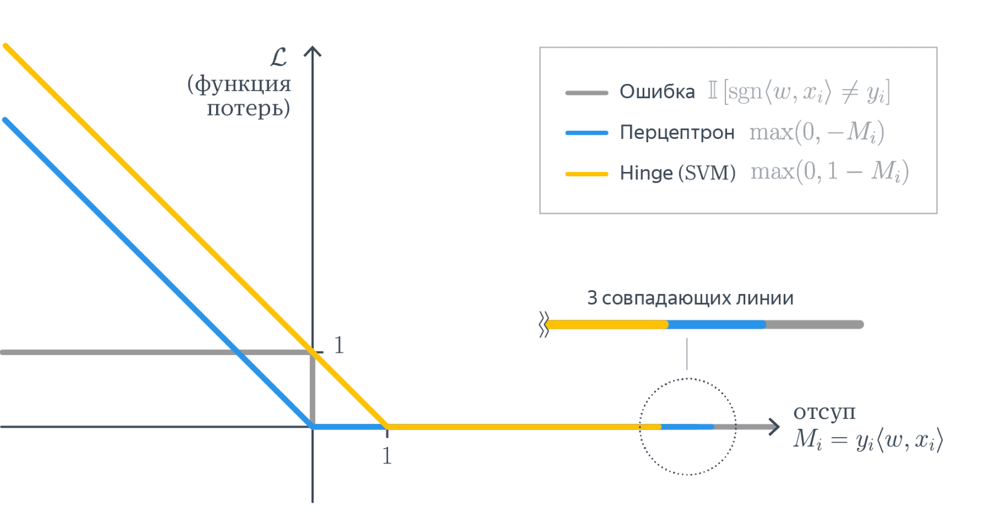
Вопрос на подумать. Допустим, мы как-то обучили классификатор, и подавляющее большинство отступов оказались отрицательными. Правда ли нас постигла катастрофа?
Ответ (не открывайте сразу; сначала подумайте сами!)Наверное, мы что-то сделали не так, но ситуацию можно локально выправить, если предсказывать классы, противоположные тем, которые выдаёт наша модель.
Вопрос на подумать. Предположим, что у нас есть два классификатора с примерно одинаковыми и достаточно приемлемыми значениями интересующей нас метрики. При этом одна почти всегда выдаёт предсказания с большими по модулю отступами, а вторая – с относительно маленькими. Верно ли, что первая модель лучше, чем вторая?
Ответ (не открывайте сразу; сначала подумайте сами!)На первый взгляд кажется, что первая модель действительно лучше: ведь она предсказывает «увереннее», но на самом деле всё не так однозначно: во многих случаях модель, которая умеет «честно признать, что не очень уверена в ответе», может быть предпочтительней модели, которая врёт с той же непотопляемой уверенностью, что и говорит правду. В некоторых случаях лучше может оказаться модель, которая, по сути, просто отказывается от классификации на каких-то объектах.
Ошибка перцептрона
Реализуем простейшую идею: давайте считать отступы только на неправильно классифицированных объектах и учитывать их не бинарно, а линейно, пропорционально их размеру. Получается такая функция:
$$F(M) = max(0, -M)$$
Давайте запишем такой лосс с $L^2$-регуляризацией:
$$L(w, x, y) = lambdavertvert wvertvert^2_2 + sum_i max(0, -y_i langle w, x_irangle)$$
Найдём градиент:
$$
nabla_w L(w, x, y) = 2 lambda w + sum_i
begin{cases}
0, & y_i langle w, x_i rangle > 0 \
— y_i x_i, & y_i langle w, x_i rangle leq 0
end{cases}
$$
Имея аналитическую формулу для градиента, мы теперь можем так же, как и раньше, применить стохастический градиентный спуск, и задача будет решена.
Данная функция потерь впервые была предложена для перцептрона Розенблатта, первой вычислительной модели нейросети, которая в итоге привела к появлению глубокого обучения.
Она решает задачу линейной классификации, но у неё есть одна особенность: её решение не единственно и сильно зависит от начальных параметров. Например, все изображённые ниже классификаторы имеют одинаковый нулевой лосс:
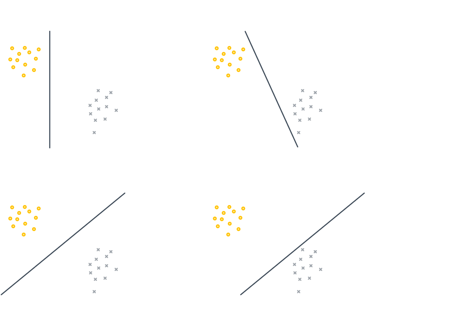
Hinge loss, SVM
Для таких случаев, как на картинке выше, возникает логичное желание не только найти разделяющую прямую, но и постараться провести её на одинаковом удалении от обоих классов, то есть максимизировать минимальный отступ:

Это можно сделать, слегка поменяв функцию ошибки, а именно положив её равной:
$$F(M) = max(0, 1-M)$$
$$L(w, x, y) = lambda||w||^2_2 + sum_i max(0, 1-y_i langle w, x_irangle)$$
$$
nabla_w L(w, x, y) = 2 lambda w + sum_i
begin{cases}
0, & 1 — y_i langle w, x_i rangle leq 0 \
— y_i x_i, & 1 — y_i langle w, x_i rangle > 0
end{cases}
$$
Почему же добавленная единичка приводит к желаемому результату?
Интуитивно это можно объяснить так: объекты, которые проклассифицированы правильно, но не очень «уверенно» (то есть $0 leq y_i langle w, x_irangle < 1$), продолжают вносить свой вклад в градиент и пытаются «отодвинуть» от себя разделяющую плоскость как можно дальше.
К данному выводу можно прийти и чуть более строго; для этого надо совершенно по-другому взглянуть на выражение, которое мы минимизируем. Поможет вот эта картинка:
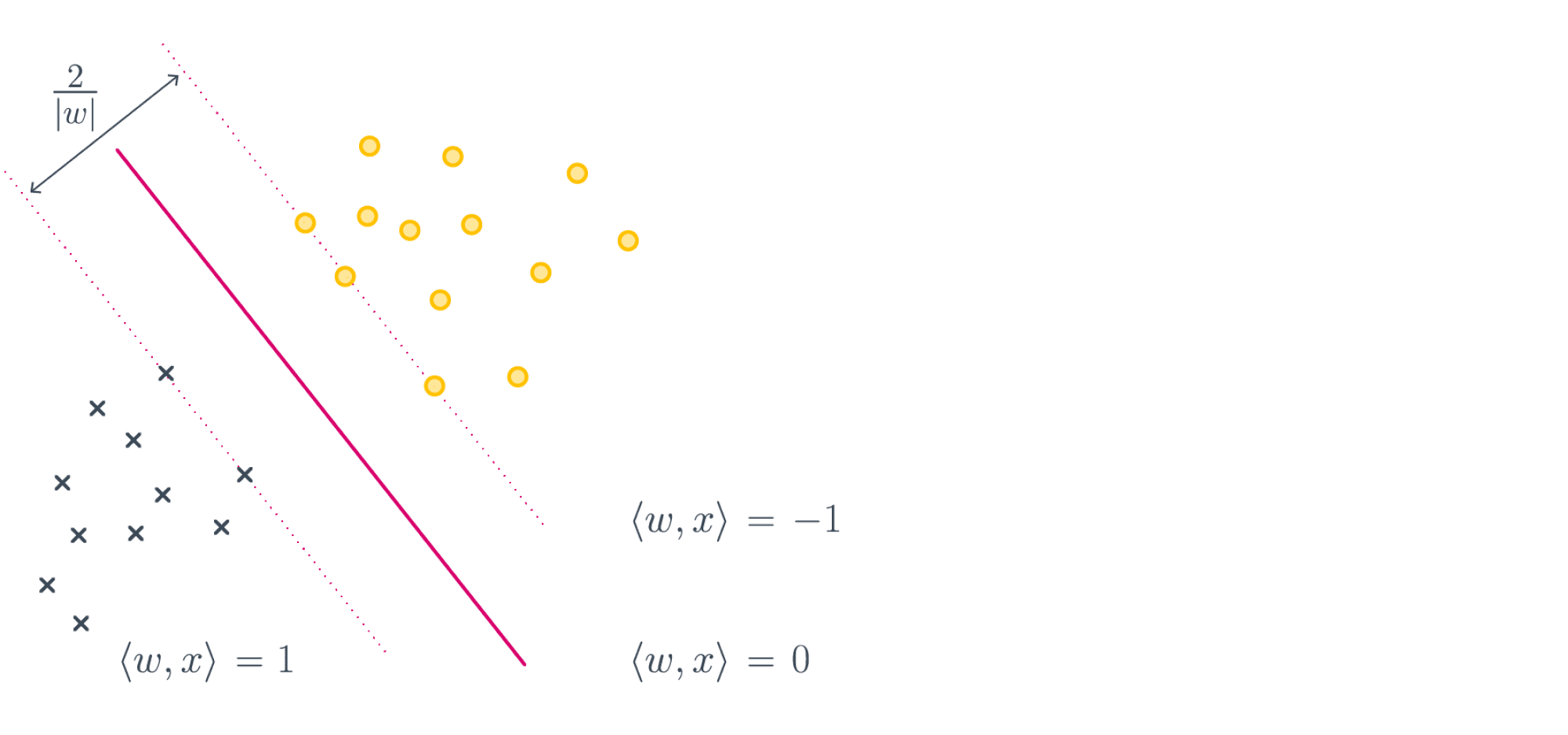
Если мы максимизируем минимальный отступ, то надо максимизировать $frac{2}{|w|_2}$, то есть ширину полосы при условии того, что большинство объектов лежат с правильной стороны, что эквивалентно решению нашей исходной задачи:
$$lambda|w|^2_2 + sum_i max(0, 1-y_i langle w, x_irangle) longrightarrowminlimits_{w}$$
Отметим, что первое слагаемое у нас обратно пропорционально ширине полосы, но мы и максимизацию заменили на минимизацию, так что тут всё в порядке. Второе слагаемое – это штраф за то, что некоторые объекты неправильно расположены относительно разделительной полосы. В конце концов, никто нам не обещал, что классы наши линейно разделимы и можно провести оптимальную плоскость вообще без ошибок.
Итоговое положение плоскости задаётся всего несколькими обучающими примерами. Это ближайшие к плоскости правильно классифицированные объекты, которые называют опорными векторами или support vectors. Весь метод, соответственно, зовётся методом опорных векторов, или support vector machine, или сокращённо SVM. Начиная с шестидесятых годов это был сильнейший из известных методов машинного обучения. В девяностые его сменили методы, основанные на деревьях решений, которые, в свою очередь, недавно передали «пальму первенства» нейросетям.
Почему же SVM был столь популярен? Из-за небольшого количества параметров и доказуемой оптимальности. Сейчас для нас нормально выбирать специальный алгоритм под задачу и подбирать оптимальные гиперпараметры для этого алгоритма перебором, а когда-то трава была зеленее, а компьютеры медленнее, и такой роскоши у людей не было. Поэтому им нужны были модели, которые гарантированно неплохо работали бы в любой ситуации. Такой моделью и был SVM.
Другие замечательные свойства SVM: существование уникального решения и доказуемо минимальная склонность к переобучению среди всех популярных классов линейных классификаторов. Кроме того, несложная модификация алгоритма, ядровый SVM, позволяет проводить нелинейные разделяющие поверхности.
Строгий вывод постановки задачи SVM можно прочитать тут или в лекции К.В. Воронцова.
Логистическая регрессия
В этом параграфе мы будем обозначать классы нулём и единицей.
Ещё один интересный метод появляется из желания посмотреть на классификацию как на задачу предсказания вероятностей. Хороший пример – предсказание кликов в интернете (например, в рекламе и поиске). Наличие клика в обучающем логе не означает, что, если повторить полностью условия эксперимента, пользователь обязательно кликнет по объекту опять. Скорее у объектов есть какая-то «кликабельность», то есть истинная вероятность клика по данному объекту. Клик на каждом обучающем примере является реализацией этой случайной величины, и мы считаем, что в пределе в каждой точке отношение положительных и отрицательных примеров должно сходиться к этой вероятности.
Проблема состоит в том, что вероятность, по определению, величина от 0 до 1, а простого способа обучить линейную модель так, чтобы это ограничение соблюдалось, нет. Из этой ситуации можно выйти так: научить линейную модель правильно предсказывать какой-то объект, связанный с вероятностью, но с диапазоном значений $(-infty,infty)$, и преобразовать ответы модели в вероятность. Таким объектом является logit или log odds – логарифм отношения вероятности положительного события к отрицательному $logleft(frac{p}{1-p}right)$.
Если ответом нашей модели является $logleft(frac{p}{1-p}right)$, то искомую вероятность посчитать не трудно:
$$langle w, x_irangle = logleft(frac{p}{1-p}right)$$
$$e^{langle w, x_irangle} = frac{p}{1-p}$$
$$p=frac{1}{1 + e^{-langle w, x_irangle}}$$
Функция в правой части называется сигмоидой и обозначается
$$color{#348FEA}{sigma(z) = frac1{1 + e^{-z}}}$$
Таким образом, $p = sigma(langle w, x_irangle)$
Как теперь научиться оптимизировать $w$ так, чтобы модель как можно лучше предсказывала логиты? Нужно применить метод максимума правдоподобия для распределения Бернулли. Это самое простое распределение, которое возникает, к примеру, при бросках монетки, которая орлом выпадает с вероятностью $p$. У нас только событием будет не орёл, а то, что пользователь кликнул на объект с такой вероятностью. Если хотите больше подробностей, почитайте про распределение Бернулли в теоретическом минимуме.
Правдоподобие позволяет понять, насколько вероятно получить данные значения таргета $y$ при данных $X$ и весах $w$. Оно имеет вид
$$ p(ymid X, w) =prod_i p(y_imid x_i, w) $$
и для распределения Бернулли его можно выписать следующим образом:
$$ p(ymid X, w) =prod_i p_i^{y_i} (1-p_i)^{1-y_i} $$
где $p_i$ – это вероятность, посчитанная из ответов модели. Оптимизировать произведение неудобно, хочется иметь дело с суммой, так что мы перейдём к логарифмическому правдоподобию и подставим формулу для вероятности, которую мы получили выше:
$$ ell(w, X, y) = sum_i big( y_i log(p_i) + (1-y_i)log(1-p_i) big) =$$
$$ =sum_i big( y_i log(sigma(langle w, x_i rangle)) + (1-y_i)log(1 — sigma(langle w, x_i rangle)) big) $$
Если заметить, что
$$
sigma(-z) = frac{1}{1 + e^z} = frac{e^{-z}}{e^{-z} + 1} = 1 — sigma(z),
$$
то выражение можно переписать проще:
$$
ell(w, X, y)=sum_i big( y_i log(sigma(langle w, x_i rangle)) + (1 — y_i) log(sigma(-langle w, x_i rangle)) big)
$$
Нас интересует $w$, для которого правдоподобие максимально. Чтобы получить функцию потерь, которую мы будем минимизировать, умножим его на минус один:
$$color{#348FEA}{L(w, X, y) = -sum_i big( y_i log(sigma(langle w, x_i rangle)) + (1 — y_i) log(sigma(-langle w, x_i rangle)) big)}$$
В отличие от линейной регрессии, для логистической нет явной формулы решения. Деваться некуда, будем использовать градиентный спуск. К счастью, градиент устроен очень просто:
$$
nabla_w L(y, X, w) = -sum_i x_i big( y_i — sigma(langle w, x_i rangle)) big)
$$
Вывод формулы градиентаНам окажется полезным ещё одно свойство сигмоиды::
$$
frac{d log sigma(z)}{d z} = left( log left( frac{1}{1 + e^{-z}} right) right)’ = frac{e^{-z}}{1 + e^{-z}} = sigma(-z)
frac{d log sigma(-z)}{d z} = -sigma(z)
$$
Отсюда:
$$
nabla_w log sigma(langle w, x_i rangle) = sigma(-langle w, x_i rangle) x_i
nabla_w log sigma(-langle w, x_i rangle) = -sigma(langle w, x_i rangle) x_i
$$
и градиент оказывается равным
$$
nabla_w L(y, X, w) = -sum_i big( y_i x_i sigma(-langle w, x_i rangle) — (1 — y_i) x_i sigma(langle w, x_i rangle)) big) =
= -sum_i big( y_i x_i (1 — sigma(langle w, x_i rangle)) — (1 — y_i) x_i sigma(langle w, x_i rangle)) big) =
= -sum_i big( y_i x_i — y_i x_i sigma(langle w, x_i rangle) — x_i sigma(langle w, x_i rangle) + y_i x_i sigma(langle w, x_i rangle)) big) =
= -sum_i big( y_i x_i — x_i sigma(langle w, x_i rangle)) big)
$$
Предсказание модели будет вычисляться, как мы договаривались, следующим образом:
$$p=sigma(langle w, x_irangle)$$
Это вероятность положительного класса, а как от неё перейти к предсказанию самого класса? В других методах нам достаточно было посчитать знак предсказания, но теперь все наши предсказания положительные и находятся в диапазоне от 0 до 1. Что же делать? Интуитивным и не совсем (и даже совсем не) правильным является ответ «взять порог 0.5». Более корректным будет подобрать этот порог отдельно, для уже построенной регрессии минимизируя нужную вам метрику на отложенной тестовой выборке. Например, сделать так, чтобы доля положительных и отрицательных классов примерно совпадала с реальной.
Отдельно заметим, что метод называется логистической регрессией, а не логистической классификацией именно потому, что предсказываем мы не классы, а вещественные числа – логиты.
Вопрос на подумать. Проверьте, что, если метки классов – это $pm1$, а не $0$ и $1$, то функцию потерь для логистической регрессии можно записать в более компактном виде:
$$mathcal{L}(w, X, y) = sum_{i=1}^Nlog(1 + e^{-y_ilangle w, x_irangle})$$
Вопрос на подумать. Правда ли разделяющая поверхность модели логистической регрессии является гиперплоскостью?
Ответ (не открывайте сразу; сначала подумайте сами!)Разделяющая поверхность отделяет множество точек, которым мы присваиваем класс $0$ (или $-1$), и множество точек, которым мы присваиваем класс $1$. Представляется логичным провести отсечку по какому-либо значению предсказанной вероятности. Однако, выбор этого значения — дело не очевидное. Как мы увидим в главе про калибровку классификаторов, это может быть не настоящая вероятность. Допустим, мы решили провести границу по значению $frac12$. Тогда разделяющая поверхность как раз задаётся равенством $p = frac12$, что равносильно $langle w, xrangle = 0$. А это гиперплоскость.
Вопрос на подумать. Допустим, что матрица объекты-признаки $X$ имеет полный ранг по столбцам (то есть все её столбцы линейно независимы). Верно ли, что решение задачи восстановления логистической регрессии единственно?
Ответ (не открывайте сразу; сначала подумайте сами!)В этот раз хорошего геометрического доказательства, как было для линейной регрессии, пожалуй, нет; нам придётся честно посчитать вторую производную и доказать, что она является положительно определённой. Сделаем это для случая, когда метки классов – это $pm1$. Формулы так получатся немного попроще. Напомним, что в этом случае
$$L(w, X, y) = -sum_{i=1}^Nlog(1 + e^{-y_ilangle w, x_irangle})$$
Следовательно,
$$frac{partial}{partial w_{j}}L(w, X, y) = sum_{i=1}^Nfrac{y_ix_{ij}e^{-y_ilangle w, x_irangle}}{1 + e^{-y_ilangle w, x_irangle}} = sum_{i=1}^Ny_ix_{ij}left(1 — frac1{1 + e^{-y_ilangle w, x_irangle}}right)$$
$$frac{partial^2L}{partial w_jpartial w_k}(w, X, y) = sum_{i=1}^Ny^2_ix_{ij}x_{ik}frac{e^{-y_ilangle w, x_irangle}}{(1 + e^{-y_ilangle w, x_irangle})^2} =$$
$$ = sum_{i=1}^Ny^2_ix_{ij}x_{ik}sigma(y_ilangle w, x_irangle)(1 — sigma(y_ilangle w, x_irangle))$$
Теперь заметим, что $y_i^2 = 1$ и что, если обозначить через $D$ диагональную матрицу с элементами $sigma(y_ilangle w, x_irangle)(1 — sigma(y_ilangle w, x_irangle))$ на диагонали, матрицу вторых производных можно представить в виде:
$$nabla^2L = left(frac{partial^2mathcal{L}}{partial w_jpartial w_k}right) = X^TDX$$
Так как $0 < sigma(y_ilangle w, x_irangle) < 1$, у матрицы $D$ на диагонали стоят положительные числа, из которых можно извлечь квадратные корни, представив $D$ в виде $D = D^{1/2}D^{1/2}$. В свою очередь, матрица $X$ имеет полный ранг по столбцам. Стало быть, для любого вектора приращения $une 0$ имеем
$$u^TX^TDXu = u^TX^T(D^{1/2})^TD^{1/2}Xu = vert D^{1/2}Xu vert^2 > 0$$
Таким образом, функция $L$ выпукла вниз как функция от $w$, и, соответственно, точка её экстремума непременно будет точкой минимума.
А теперь – почему это не совсем правда. Дело в том, что, говоря «точка её экстремума непременно будет точкой минимума», мы уже подразумеваем существование этой самой точки экстремума. Только вот существует этот экстремум не всегда. Можно показать, что для линейно разделимой выборки функция потерь логистической регрессии не ограничена снизу, и, соответственно, никакого экстремума нет. Доказательство мы оставляем читателю.
Вопрос на подумать. На картинке ниже представлены результаты работы на одном и том же датасете трёх моделей логистической регрессии с разными коэффициентами $L^2$-регуляризации:
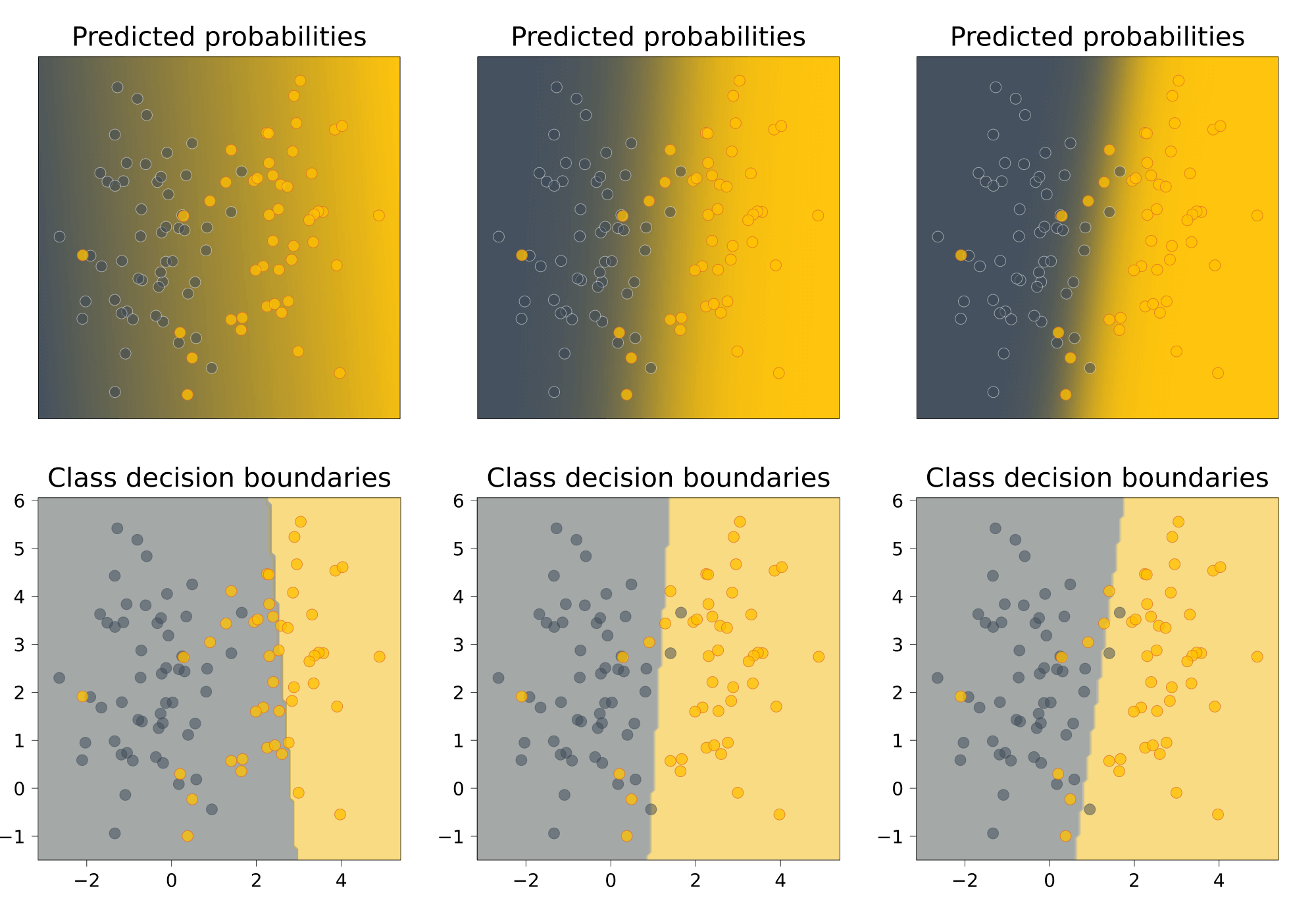
Наверху показаны предсказанные вероятности положительного класса, внизу – вид разделяющей поверхности.
Как вам кажется, какие картинки соответствуют самому большому коэффициенту регуляризации, а какие – самому маленькому? Почему?
Ответ (не открывайте сразу; сначала подумайте сами!)Коэффициент регуляризации максимален у левой модели. На это нас могут натолкнуть два соображения. Во-первых, разделяющая прямая проведена достаточно странно, то есть можно заподозрить, что регуляризационный член в лосс-функции перевесил функцию потерь исходной задачи. Во-вторых, модель предсказывает довольно близкие к $frac12$ вероятности – это значит, что значения $langle w, xrangle$ близки к нулю, то есть сам вектор $w$ близок к нулевому. Это также свидетельствует о том, что регуляризационный член играет слишком важную роль при оптимизации.
Наименьший коэффициент регуляризации у правой модели. Её предсказания достаточно «уверенные» (цвета на верхнем графике сочные, то есть вероятности быстро приближаются к $0$ или $1$). Это может свидетельствовать о том, что числа $langle w, xrangle$ достаточно велики по модулю, то есть $vertvert w vertvert$ достаточно велик.
Многоклассовая классификация
В этом разделе мы будем следовать изложению из лекций Евгения Соколова.
Пусть каждый объект нашей выборки относится к одному из $K$ классов: $mathbb{Y} = {1, ldots, K}$. Чтобы предсказывать эти классы с помощью линейных моделей, нам придётся свести задачу многоклассовой классификации к набору бинарных, которые мы уже хорошо умеем решать. Мы разберём два самых популярных способа это сделать – one-vs-all и all-vs-all, а проиллюстрировать их нам поможет вот такой игрушечный датасет
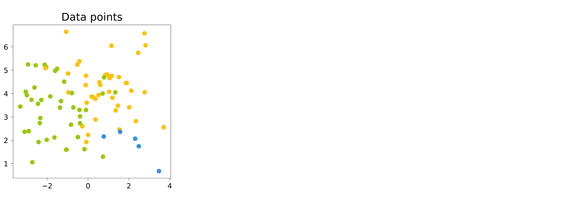
Один против всех (one-versus-all)
Обучим $K$ линейных классификаторов $b_1(x), ldots, b_K(x)$, выдающих оценки принадлежности классам $1, ldots, K$ соответственно. В случае с линейными моделями эти классификаторы будут иметь вид
$$b_k(x) = text{sgn}left(langle w_k, x rangle + w_{0k}right)$$
Классификатор с номером $k$ будем обучать по выборке $left(x_i, 2mathbb{I}[y_i = k] — 1right)_{i = 1}^{N}$; иными словами, мы учим классификатор отличать $k$-й класс от всех остальных.
Логично, чтобы итоговый классификатор выдавал класс, соответствующий самому уверенному из бинарных алгоритмов. Уверенность можно в каком-то смысле измерить с помощью значений линейных функций:
$$a(x) = text{argmax}_k left(langle w_k, x rangle + w_{0k}right) $$
Давайте посмотрим, что даст этот подход применительно к нашему датасету. Обучим три линейных модели, отличающих один класс от остальных:

Теперь сравним значения линейных функций
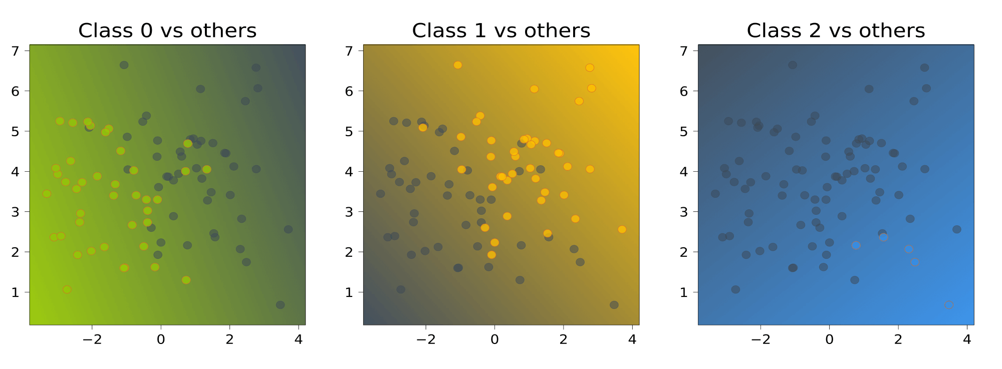
и для каждой точки выберем тот класс, которому соответствует большее значение, то есть самый «уверенный» классификатор:
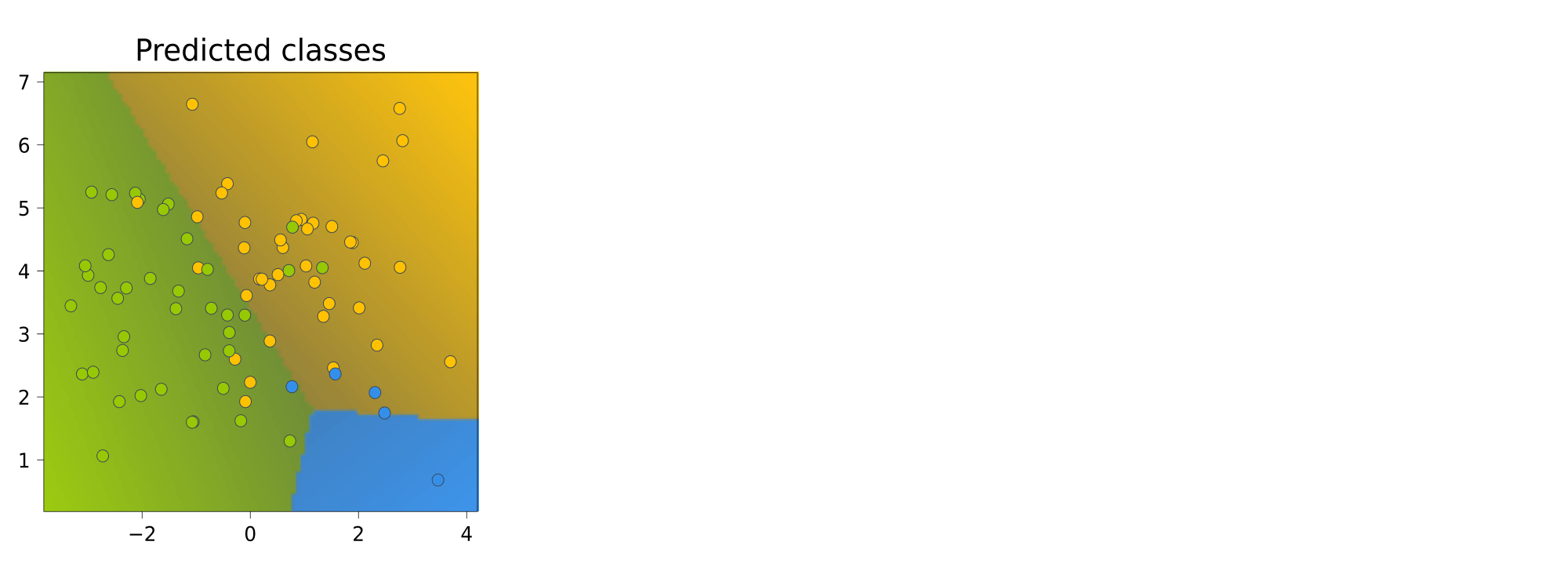
Хочется сказать, что самый маленький класс «обидели».
Проблема данного подхода заключается в том, что каждый из классификаторов $b_1(x), dots, b_K(x)$ обучается на своей выборке, и значения линейных функций $langle w_k, x rangle + w_{0k}$ или, проще говоря, «выходы» классификаторов могут иметь разные масштабы. Из-за этого сравнивать их будет неправильно. Нормировать вектора весов, чтобы они выдавали ответы в одной и той же шкале, не всегда может быть разумным решением: так, в случае с SVM веса перестанут являться решением задачи, поскольку нормировка изменит норму весов.
Все против всех (all-versus-all)
Обучим $C_K^2$ классификаторов $a_{ij}(x)$, $i, j = 1, dots, K$, $i neq j$. Например, в случае с линейными моделями эти модели будут иметь вид
$$b_{ij}(x) = text{sgn}left( langle w_{ij}, x rangle + w_{0,ij} right)$$
Классификатор $a_{ij}(x)$ будем настраивать по подвыборке $X_{ij} subset X$, содержащей только объекты классов $i$ и $j$. Соответственно, классификатор $a_{ij}(x)$ будет выдавать для любого объекта либо класс $i$, либо класс $j$. Проиллюстрируем это для нашей выборки:
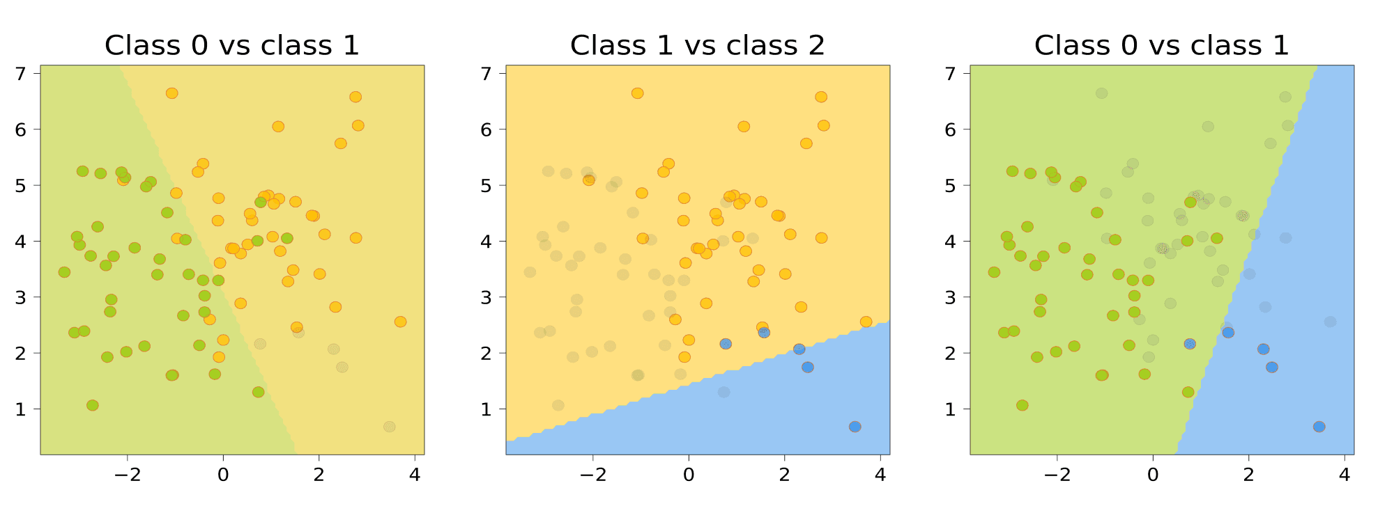
Чтобы классифицировать новый объект, подадим его на вход каждого из построенных бинарных классификаторов. Каждый из них проголосует за своей класс; в качестве ответа выберем тот класс, за который наберется больше всего голосов:
$$a(x) = text{argmax}_ksum_{i = 1}^{K} sum_{j neq i}mathbb{I}[a_{ij}(x) = k]$$
Для нашего датасета получается следующая картинка:
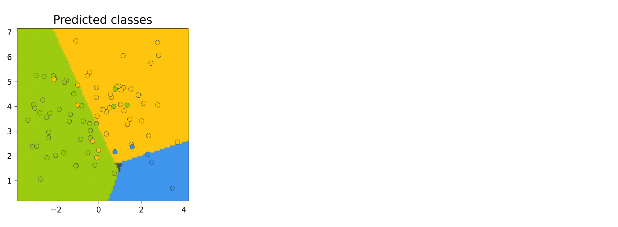
Обратите внимание на серый треугольник на стыке областей. Это точки, для которых голоса разделились (в данном случае каждый классификатор выдал какой-то свой класс, то есть у каждого класса было по одному голосу). Для этих точек нет явного способа выдать обоснованное предсказание.
Многоклассовая логистическая регрессия
Некоторые методы бинарной классификации можно напрямую обобщить на случай многих классов. Выясним, как это можно проделать с логистической регрессией.
В логистической регрессии для двух классов мы строили линейную модель
$$b(x) = langle w, x rangle + w_0,$$
а затем переводили её прогноз в вероятность с помощью сигмоидной функции $sigma(z) = frac{1}{1 + exp(-z)}$. Допустим, что мы теперь решаем многоклассовую задачу и построили $K$ линейных моделей
$$b_k(x) = langle w_k, x rangle + w_{0k},$$
каждая из которых даёт оценку принадлежности объекта одному из классов. Как преобразовать вектор оценок $(b_1(x), ldots, b_K(x))$ в вероятности? Для этого можно воспользоваться оператором $text{softmax}(z_1, ldots, z_K)$, который производит «нормировку» вектора:
$$text{softmax}(z_1, ldots, z_K) = left(frac{exp(z_1)}{sum_{k = 1}^{K} exp(z_k)},
dots, frac{exp(z_K)}{sum_{k = 1}^{K} exp(z_k)}right).$$
В этом случае вероятность $k$-го класса будет выражаться как
$$P(y = k vert x, w) = frac{
exp{(langle w_k, x rangle + w_{0k})}}{ sum_{j = 1}^{K} exp{(langle w_j, x rangle + w_{0j})}}.$$
Обучать эти веса предлагается с помощью метода максимального правдоподобия: так же, как и в случае с двухклассовой логистической регрессией:
$$sum_{i = 1}^{N} log P(y = y_i vert x_i, w) to max_{w_1, dots, w_K}$$
Масштабируемость линейных моделей
Мы уже обсуждали, что SGD позволяет обучению хорошо масштабироваться по числу объектов, так как мы можем не загружать их целиком в оперативную память. А что делать, если признаков очень много, или мы не знаем заранее, сколько их будет? Такое может быть актуально, например, в следующих ситуациях:
- Классификация текстов: мы можем представить текст в формате «мешка слов», то есть неупорядоченного набора слов, встретившихся в данном тексте, и обучить на нём, например, определение тональности отзыва в интернете. Наличие каждого слова из языка в тексте у нас будет кодироваться отдельной фичой. Тогда размерность каждого элемента обучающей выборки будет порядка нескольких сотен тысяч.
- В задаче предсказания кликов по рекламе можно получить выборку любой размерности, например, так: в качестве фичи закодируем индикатор того, что пользователь X побывал на веб-странице Y. Суммарная размерность тогда будет порядка $10^9 cdot 10^7 = 10^{16}$. Кроме того, всё время появляются новые пользователи и веб-страницы, так что на этапе применения нас ждут сюрпризы.
Есть несколько хаков, которые позволяют бороться с такими проблемами:
- Несмотря на то, что полная размерность объекта в выборке огромна, количество ненулевых элементов в нём невелико. Значит, можно использовать разреженное кодирование, то есть вместо плотного вектора хранить словарь, в котором будут перечислены индексы и значения ненулевых элементов вектора.
- Даже хранить все веса не обязательно! Можно хранить их в хэш-таблице и вычислять индекс по формуле
hash(feature) % tablesize. Хэш может вычисляться прямо от слова или id пользователя. Таким образом, несколько фичей будут иметь общий вес, который тем не менее обучится оптимальным образом. Такой подход называется hashing trick. Ясно, что сжатие вектора весов приводит к потерям в качестве, но, как правило, ценой совсем небольших потерь можно сжать этот вектор на много порядков.
Примером открытой библиотеки, в которой реализованы эти возможности, является vowpal wabbit.
Parameter server
Если при решении задачи ставки столь высоки, что мы не можем разменивать качество на сжатие вектора весов, а признаков всё-таки очень много, то задачу можно решать распределённо, храня все признаки в шардированной хеш-таблице
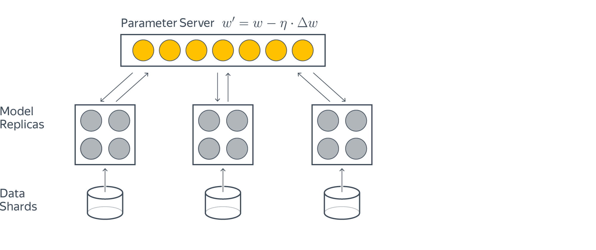
Кружки здесь означают отдельные сервера. Жёлтые загружают данные, а серые хранят части модели. Для обучения жёлтый кружок запрашивает у серого нужные ему для предсказания веса, считает градиент и отправляет его обратно, где тот потом применяется. Схема обладает бесконечной масштабируемостью, но задач, где это оправдано, не очень много.
Подытожим
На линейную модель можно смотреть как на однослойную нейросеть, поэтому многие методы, которые были изначально разработаны для них, сейчас переиспользуются в задачах глубокого обучения, а базовые подходы к регрессии, классификации и оптимизации вообще выглядят абсолютно так же. Так что несмотря на то, что в целом линейные модели на сегодня применяются редко, то, из чего они состоят и как строятся, знать очень и очень полезно.
Надеемся также, что главным итогом прочтения этой главы для вас будет осознание того, что решение любой ML-задачи состоит из выбора функции потерь, параметризованного класса моделей и способа оптимизации. В следующих главах мы познакомимся с другими моделями и оптимизаторами, но эти базовые принципы не изменятся.
Terence Parr and Jeremy
Howard
(Terence is a tech lead at Google and ex-Professor of computer/data science; both he and Jeremy teach in University of San Francisco’s MS in Data Science program and have other nefarious projects underway. You might know Terence as the creator of the ANTLR parser generator. Jeremy is a founding researcher at fast.ai, a research institute dedicated to making deep learning more accessible.)
Please send comments, suggestions, or fixes to Terence.
Contents
- Roadmap
- Distance to target
- An introduction to additive modeling
- An introduction to boosted regression
- The intuition behind gradient boosting
- Gradient boosting regression by example
- Measuring model performance
- Choosing hyper-parameters
- GBM algorithm to minimize L2 loss
- Heading in the right direction
- Chasing the sign vector
- Two perspectives on training weak models for L1 loss
- GBM optimizing MAE by example
- Comparing GBM trees that optimize MSE and MAE
- GBM algorithm to minimize L1 loss
- Gradient boosting performs gradient descent
- The intuition behind gradient descent
- Boosting as gradient descent in prediction space
- The MSE function gradient
- The MAE function gradient
- Morphing GBM into gradient descent
- Function space is prediction space
- How gradient boosting differs from gradient descent
- Summary
- General algorithm with regression tree weak models
- Frequently asked questions (FAQ)
Roadmap
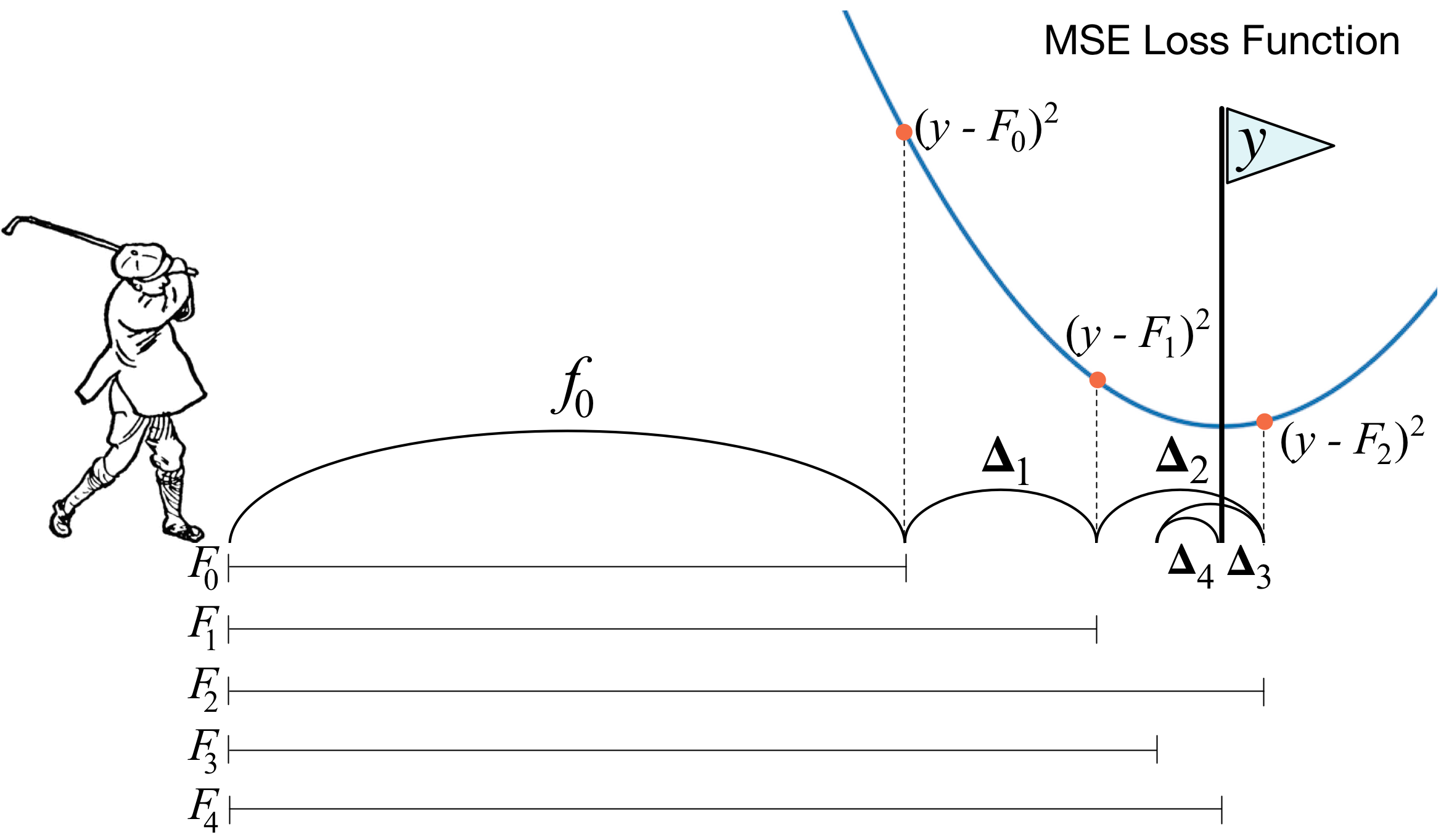 Gradient boosting machines (GBMs) are currently very popular and so it’s a good idea for machine learning practitioners to understand how GBMs work. The problem is that understanding all of the mathematical machinery is tricky and, unfortunately, these details are needed to tune the hyper-parameters. (Tuning the hyper-parameters is required to get a decent GBM model unlike, say, Random Forests.) Our goal in this article is to explain the intuition behind gradient boosting, provide visualizations for model construction, explain the mathematics as simply as possible, and answer thorny questions such as why GBM is performing “gradient descent in function space.” We’ve split the discussion into three morsels and a FAQ for easier digestion.
- Gradient boosting: Distance to target.
First, we examine the most common form of GBM that optimizes the mean squared error (MSE), also called the L2 loss or cost. (The mean squared error is the average of the square of the difference between the true targets and the predicted values from a set of observations, such as a training or validation set.) As we’ll see, A GBM is a composite model that combines the efforts of multiple weak models to create a strong model, and each additional weak model reduces the mean squared error (MSE) of the overall model. We give a fully-worked GBM example for a simple data set, complete with computations and model visualizations. - Gradient boosting: Heading in the right direction.
Optimizing a model according to MSE makes it chase outliers because squaring the difference between targets and predicted values emphasizes extreme values. When we can’t remove outliers, it’s better to optimize the mean absolute error (MAE), also called the L1 loss or cost. (The MAE is the average of the absolute value of the difference between the true targets and the predicted values.) This second article shows the computations and visualizations for a GBM that optimizes MAE for the same data set as used in the first article to optimize MSE. - Gradient boosting performs gradient descent.
The previous two articles give the intuition behind GBM and the simple formulas to show how weak models join forces to create a strong regression model. No attempt was made to show how we can abstract out a generalized GBM that works for any loss function. This last article demonstrates that gradient boosting is really doing a form of gradient descent and, therefore, is in fact optimizing MSE or MAE depending on the direction vectors we use to train the weak models. The discussion relies on a bit of derivative calculus but it’s an important read if you’d like to learn deeply how GBM works. (To brush up on your vectors and derivatives, you can check out The Matrix Calculus You Need For Deep Learning.) We finish off by clearing up a number of confusion points regarding gradient boosting.As Ben Gorman points out in A Kaggle Master Explains Gradient Boosting, “This is the part that gets butchered by a lot of gradient boosting explanations.” His blog post does a good job of explaining it, but we give our own perspective here.
- Frequently asked questions (FAQ).
There are lots of confusing things about gradient boosting machines and we have collected and answered a number of questions from students in this piece.
Recommended reading
To get started with GBM, those with very strong mathematical backgrounds can go directly to the super-tasty 1999 paper by Jerome Friedman called Greedy Function Approximation: A Gradient Boosting Machine. To get the practical and implementation perspective, though, we recommend Ben Gorman’s excellent blog A Kaggle Master Explains Gradient Boosting and Prince Grover’s Gradient Boosting from scratch (written by a data science graduate student at the University of San Francisco; we also thank Prince for reviewing this article.) To go beyond basic GBM, see XGBoost: A Scalable Tree Boosting System by Chen and Guestrin. To get really fancy, you can even add momentum to the gradient descent performed by boosting machines, as shown in the recent article: Accelerated Gradient Boosting.
Python notebooks
All of the code used to generate the graphs and data in these articles is available in the Notebooks directory at github. Warning: the code is a just good enough to generate the graphs in these articles; the code is provided purely for transparency and completeness (i.e., we ain’t proud of it).
Tricks
Linear regression involves moving a line such that it is the best approximation for a set of points. The absolute trick and square trick are techniques to move a line closer to a point.
Absolute Trick
A line with slope $w_1$ and y-intercept $w_2$ would have equation $y = w_1x + w_2$. To move the line closer to the point $(p,q)$, the application of the absolute trick involves changing the equation of the line to
$$y = (w_1 + palpha)x + (w_2 + alpha)$$
where $alpha$ is the learning rate and is a small number whose sign depends on whether the point is above or below the line.
As an example, consider a line $y = -0.6x + 4$, a point $(x,y)=(-5,3)$, and $alpha=0.1$. The point is below the line, so $alpha$ is changed to be$alpha=-0.1$. Following the application of the absolute trick, the equation of the line would be
$$y = (-0.6 + (-5)(-0.1))x + (4 — 0.1)$$
$$y = -0.1x + 3.9$$
Square Trick
A line with slope $w_1$ and y-intercept $w_2$ would have equation $y = w_1x + w_2$. The goal is to move the line closer to the point $(p,q)$. A point on the line with the same y-coordinate as $(p,q)$ might be given by $(p,q’)$. The distance between $(p,q)$ and $(p,q’)$ is given by $(q-q’)$. Following application of the square trick, the new equation would be given by
$$y = (w_1 + p(q-q’)alpha)x + (w_2 + (q-q’)alpha)$$
where $alpha$ is the learning rate and is a small number whose sign does not depend on whether the point is above or below the line. This is due to the inclusion of the $(q-q’)$ term that takes care of this implicitly.
As an example, consider a line $y = -0.6x + 4$, a point $(x,y)=(-5,3)$, and $alpha=0.01$.
$$q’ = -0.6(-5) + 4 = 3 + 4 = 7$$
$$(q — q’) = (3 — 7) = -4$$
Then, the new equation for the line would be given by
$$y = (-0.6 + (-5)(-4)(0.01))x + (4 + (-4)(0.01))$$
$$y = -0.4x + 3.96$$
Gradient Descent
The more formal way by which regression works is called gradient descent. For a given line and set of points, we can define a function that calculates an “error.” This error gives us some sense of how far the line is from the points. After moving the line, this error would be recalculated and should decrease. Gradient descent involves determining which direction to move the line that would decrease the error the most.
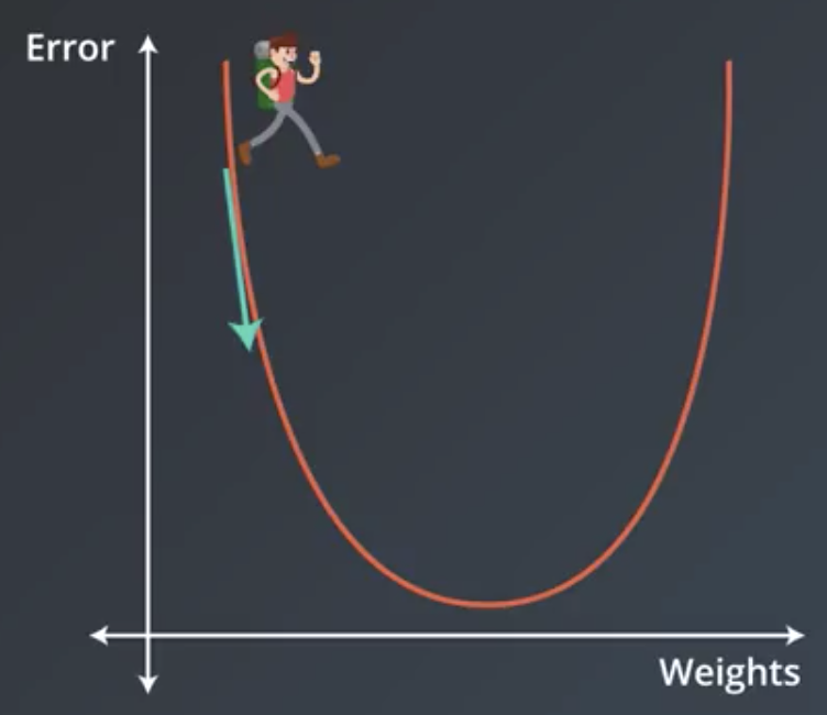
More technically, it involves taking the derivative, or gradient, of the error function with respect to the weights, and taking a step in the direction of largest decrease.
$$w_i rightarrow w_i — alpha frac{partial}{partial w_i}Error$$
Following several similar steps, the function will arrive at either a minimum or a value where the error is small. This is also referred to as “decreasing the error function by walking along the negative of its gradient.”
Mean Absolute Error
The two most common error functions for linear regression are the mean absolute error and the mean squared error. Consider a point $(x,y)$ and a line $(x,hat{y})$. The vertical distance from the point to the line is given by $y-hat{y}$.
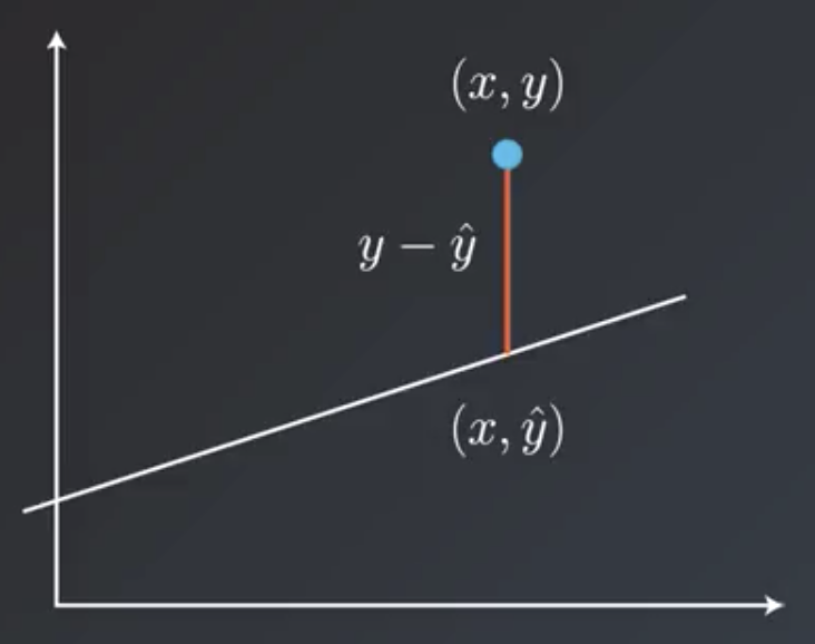
Then, the total error is the sum of all these distances from the points to the line in the dataset divided by the number of points, $m$.
$$Error = frac{1}{m} sum^m_{i=1}|y-hat{y}|$$
For example, consider the line $y = 1.2x + 2$ and the points $(2, -2), (5, 6), (-4, -4), (-7, 1), (8, 14)$:
| # | Point | $hat{y}$ | $|y — hat{y}|$ |
|---|---|---|---|
| 1 | (2, -2) | 2.4 | 6.4 |
| 2 | (5, 6) | 6 | 2 |
| 3 | (-4, -4) | -4.8 | 1.2 |
| 4 | (-7, 1) | -8.4 | 7.4 |
| 5 | (8, 14) | 9.6 | 2.4 |
$$Error = frac{1}{5} (6.4 + 2 + 1.2 + 7.4 + 2.4) = 3.88$$
Mean Squared Error
The mean squared error is similar to the mean absolute error. The extra factor of $frac{1}{2}$ is for convenience later.
$$Error = frac{1}{2m} sum^m_{i=1}(y-hat{y})^2$$
| # | Point | $hat{y}$ | ($y — hat{y})^2$ |
|---|---|---|---|
| 1 | (2, -2) | 2.4 | 40.96 |
| 2 | (5, 6) | 6 | 4 |
| 3 | (-4, -4) | -4.8 | 1.44 |
| 4 | (-7, 1) | -8.4 | 54.76 |
| 5 | (8, 14) | 9.6 | 5.76 |
$$Error = frac{1}{(2)(5)} (40.96 + 4 + 1.44 + 54.76 + 5.76) = 10.692$$
Derivative of the Error Function
The absolute trick and square trick and the mean absolute error and mean squared error are actually the same thing.
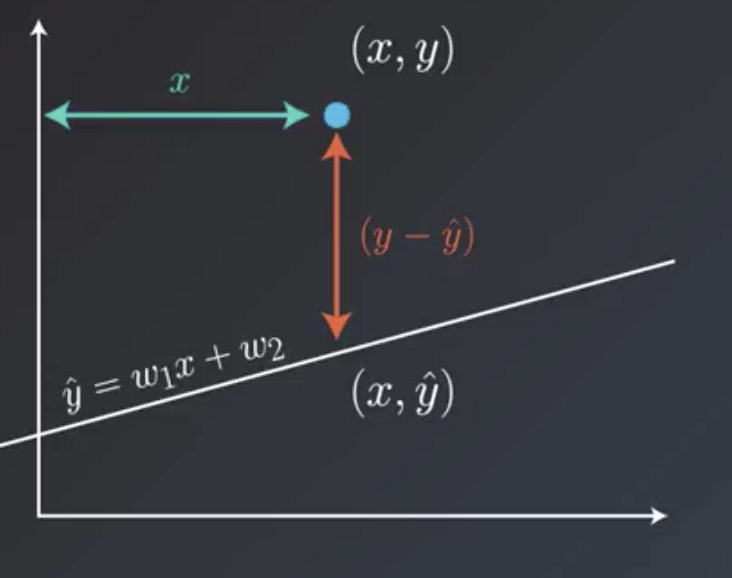
By using the square trick, we actually are taking a gradient descent step:
$$Error = frac{1}{2}(y-hat{y})^2$$
$$frac{partial}{partial w_1} Error = frac{partial Error}{partial hat{y}} frac{partial hat{y}}{partial w_1} = -(y-hat{y})x$$
$$frac{partial}{partial w_2} Error = frac{partial Error}{partial hat{y}} frac{partial hat{y}}{partial w_2} = -(y-hat{y})$$
Gradient step:
$$w_i rightarrow w_i — alpha frac{partial}{partial w_i} Error$$
By using the absolute trick, we actually are taking a gradient descent step as well.
$$Error = |y — hat{y}|$$
$$frac{partial}{partial w_1} Error = pm x$$
$$frac{partial}{partial w_2} Error = pm 1$$
The $pm$ is based on whether the point is above or below the line.
Gradient step:
$$w_i rightarrow w_i — alpha frac{partial}{partial w_i} Error$$
Mean versus Total Squared (or absolute) Error
The total squared error, $M$, is the sum of errors at each point.
$$M = sum^m_{i=1} frac{1}{2} (y — hat{y})^2$$
The mean squared error, $T$ is the average of these errors.
$$T = sum^m_{i=1} frac{1}{2m} (y — hat{y})^2$$
So, the total squared error is just a multiple of the mean squared error, because $M = mT$. When using regression in practice, algorithms help determine a good learning rate to work with. Whether the mean error or the total error is selected, it ultimately will just amount to picking a different learning rate, and the algorithms will just adjust accordingly. So, either mean or total squared error can be used.
Batch versus Stochastic versus Mini-Batch Gradient Descent
- Batch gradient descent: applying on of the tricks at every point in the data, all at the same time.
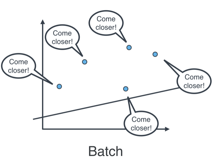
- Stochastic gradient descent: applying one of the tricks at every point in the data, one by one.
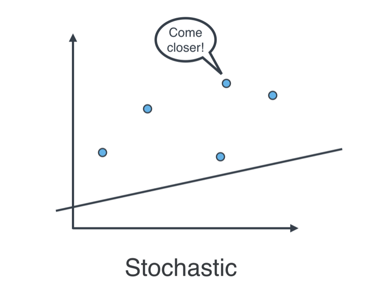
- Mini-batch gradient descent: applying one of the tricks to a small batch of points, with each small batch containing roughly the same number of points. Computationally, this is the most efficient approach, and the one that is used in practice.
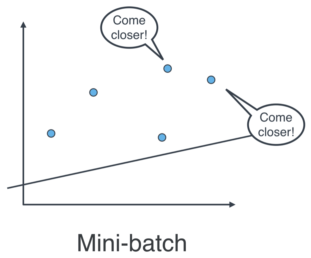
Mean Squared versus Mean Absolute Errors
One difference between these two error formulations is that the mean squared error is a quadratic function, whereas mean absolute error is not. What this means practically is that in some point distributions the mean squared error will give better results.
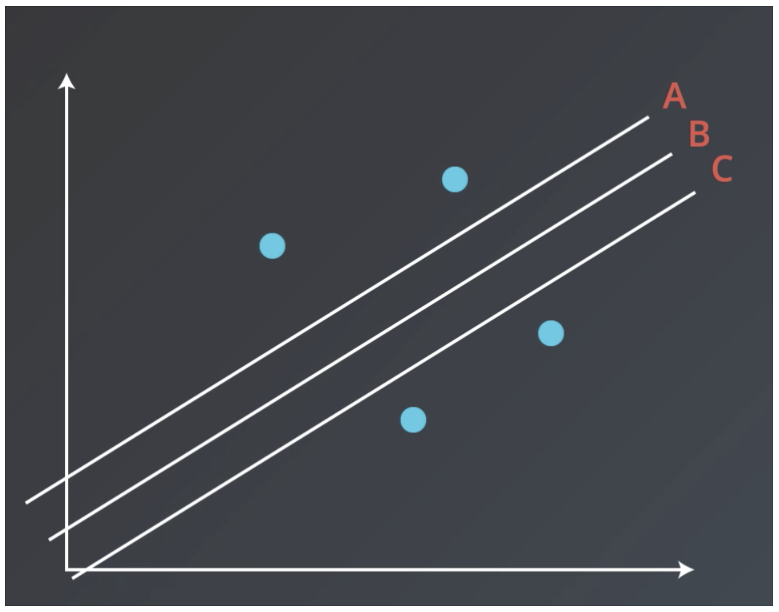
Lines A, B, and C have the same mean absolute error on the points distributions shown, but B has the smallest mean squared error.
Generalizing to Higher Dimensions
Previous examples have been two-dimensional problems. For example, a model might take as an input house size and output house price. In 2-dimensional models, the prediction is a line.
$$Price = w_1(size) + w_2$$
Consider a situation where house size and nearby school quality are both factors used by a model that predicts house price. In this situation, the graph becomes 2-dimensional, and the prediction becomes a plane.
$$Price = w_1(school quality) + w_2(size) + w_3$$
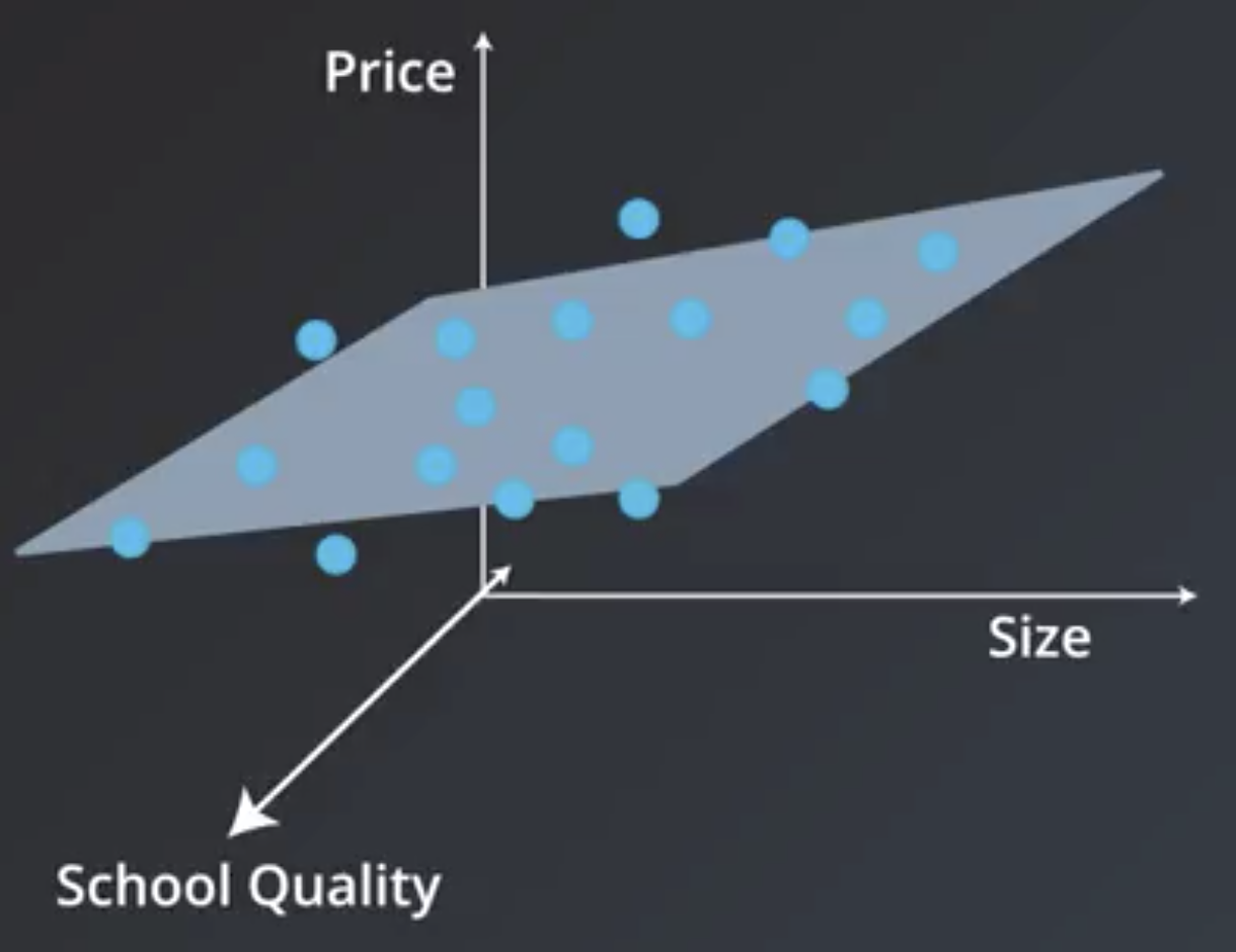
In the more general $n$-dimensional case there are $n-1$ input features ($x_1, x_2, …, x_{n-1}$, also known as predictors or independent variables) and $1$ output feature ($hat{y}$, also known as dependent variables). The prediction becomes an $n-1$ dimensional hyperplane.
$$hat{y} = w_1 x_1 + w_2 x_2 + … + w_{n-1} x_{n-1} + w_n$$
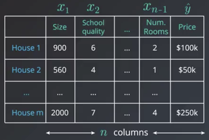
The algorithm in this more general situation is exactly the same as the 2-dimensional case.
The instructor notes that there is actually a closed form solution to finding the set of coefficients, $w_1, … w_{n-1}$, that give the minimum mean squared error. Using this closed form solution requires solving a system of $n$ equations and $n$ unknowns, however, which, depending on the dataset, may be computationally expensive to the point of being impractical. So, in practice, gradient descent is almost always used. It does not give an exact answer in the same way that a closed-form solution would, but the approximate solution it does provide is almost always adequate.
Linear Regression Warnings
Linear regression comes with a set of implicit assumptions and is not the best model for every situation.
Linear Regression Works Best when the Data is Linear
If the relationship is not linear, then you can:
- Make adjustments (transform the data),
- Add features, or
- Use another kind of model.
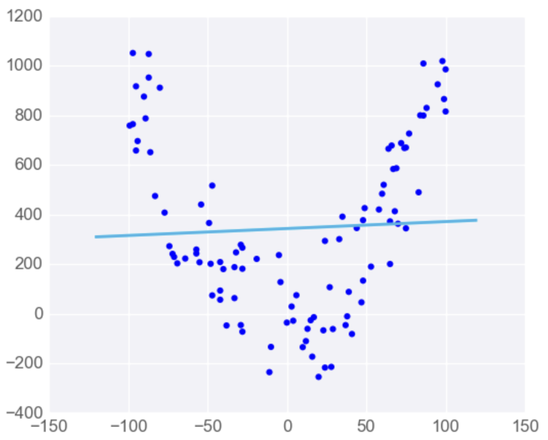
Linear Regression is Sensitive to Outliers
If the dataset has some outlying extreme values that don’t fit a general pattern, they can have a very large effect.
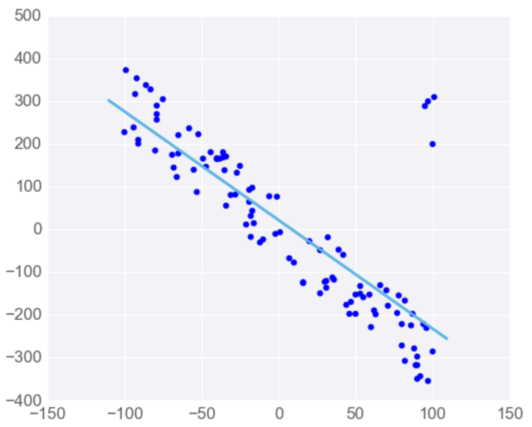
Polynomial Regression
Some datasets are clearly not suited to linear regression. a polynomial may work better.
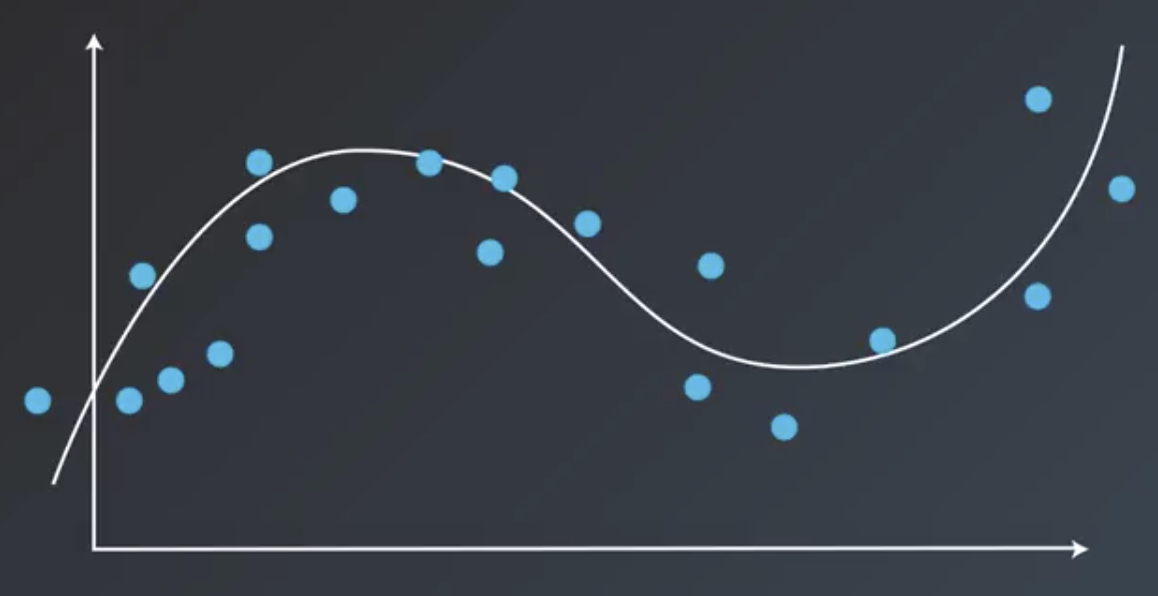
In these situations, instead of a line, a polynomial like the following could be used instead.
$$hat{y} = w_1 x^3 + w_2 x^2 + w_3 x + w_4$$
The algorithm to solve this equation is the exact same thing. We take the mean absolute or mean squared error and take the derivative with the four variables. Then, we use gradient descent to modify these four weights and minimize the error. This algorithm is known as polynomial regression.
Regularization
Regularization is a concept that works for both classification and regression. It is a technique to improve our models and make sure they don’t overfit.
In machine learning, there is often a tradeoff between accuracy and generalizability. In the image below, the linear model is not as accurate as the polynomial. Specifically, the linear model makes two misclassifications. But, the linear model is simpler and may generalize better to other datasets better than the polynomial model, which is more complex and accurate but may be overfit to this particular dataset.
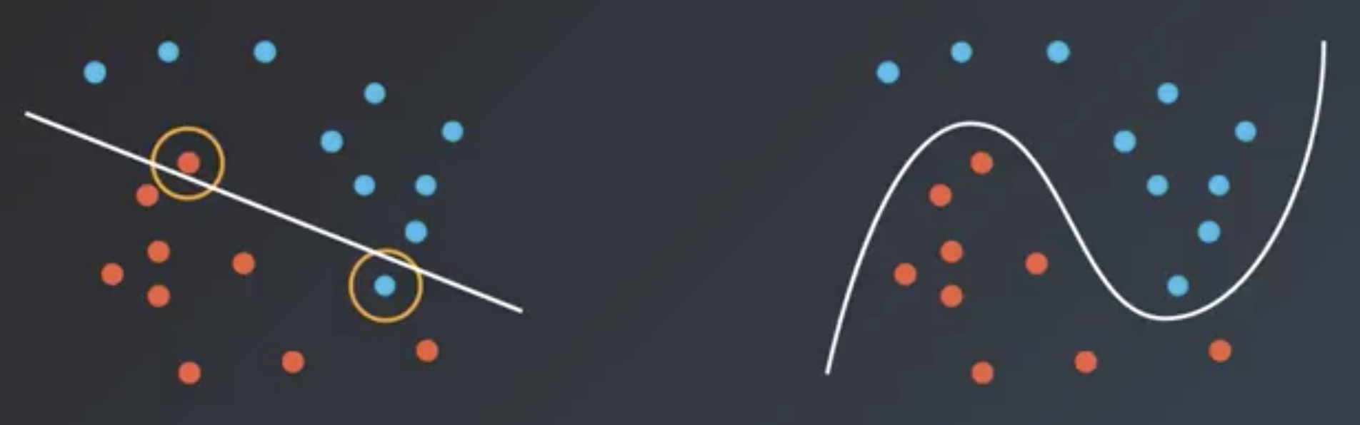
Regularization is a way to take the complexity of the model into account when calculating the overall error of the model. So, the overall error of a given model is redefined as any misclassifications plus the complexity of the model.
L1 Regularization
In L1 Regularization, the absolute value of the coefficients is added to the error.
For example, in the case of the following polynomial model:
$$2 x_1^3 — 2 x_1^2 x_2 — 4 x_2^3 + 3 x_1^2 + 6 x_1 x_2 + 4 x_2^2 + 5 = 0$$
$$Error = |2| + |-2| + |-4| + |3| + |6| + |4| = 21$$
In the case of the following linear model:
$$3 x_1 — 4 x_2 + 5 = 0$$
$$Error = |3| + |4| = 7$$
L2 Regularization
L2 Regularization is similar, except it involves adding the squares of the coefficients.
For the same polynomial above:
$$Error = 2^2 + (-2)^2 + (-4)^2 + 3^2 + 6^2 + 4^2 = 85$$
For the same linear model above:
$$Error = 3^2 + 4^2 = 25$$
Regularization Tradeoffs
The type of regularization to use depends on the model’s use-case. If the model will be used in medical or aerospace applications, maybe low error is required and high complexity is okay. If the model is used to recommend videos or friends on a social networking site, maybe scalability and therefore simplicity and speed need to be prioritized.
The amount of regularization applied to an algorithm is determined by a parameter called lambda ($lambda$), which is a scalar by which the regularization term is multiplied.
| L1 Regularization | L2 Regularization |
|---|---|
| Computationally Inefficient (unless data is sparse) | Computationally Efficient |
| Sparse Outputs | Non-Sparse Outputs |
| Feature Selection (may set some features to 0) | No Feature Selection |
Feature Scaling
Feature scaling is a way of transforming data into a common range of values. There are two common scalings: standardizing and normalizing.
Standardizing
Standardizing is the most common technique for feature scaling. Data is standardized by subtracting the mean of each column from each value, then dividing it by the standard deviation of the column.
df["height_standard"] = (df["height"] - df["height"].mean()) / df["height"].std()
Normalizing
Normalizing is performed by scaling data to a value between 0 and 1.
df["height_normal"] = (df["height"] - df["height"].min()) / (df["height"].max() - df['height'].min())
When Should Feature Scaling be Used?
- When the algorithm uses a distance-based metric to predict
- For example, Support Vector Machines and K-Nearest Neighbors (K-NN) both require that the input data be scaled.
- When using regularization
- For example, when one feature is on a small range (0-10) and another is on a large range (0-1000), regularization will unduly punish the feature with the small range.
- Note that feature scaling can also speed up convergence of machine learning algorithms, which may be an important consideration.