From Wikipedia, the free encyclopedia
In statistics, the mean squared error (MSE)[1] or mean squared deviation (MSD) of an estimator (of a procedure for estimating an unobserved quantity) measures the average of the squares of the errors—that is, the average squared difference between the estimated values and the actual value. MSE is a risk function, corresponding to the expected value of the squared error loss.[2] The fact that MSE is almost always strictly positive (and not zero) is because of randomness or because the estimator does not account for information that could produce a more accurate estimate.[3] In machine learning, specifically empirical risk minimization, MSE may refer to the empirical risk (the average loss on an observed data set), as an estimate of the true MSE (the true risk: the average loss on the actual population distribution).
The MSE is a measure of the quality of an estimator. As it is derived from the square of Euclidean distance, it is always a positive value that decreases as the error approaches zero.
The MSE is the second moment (about the origin) of the error, and thus incorporates both the variance of the estimator (how widely spread the estimates are from one data sample to another) and its bias (how far off the average estimated value is from the true value).[citation needed] For an unbiased estimator, the MSE is the variance of the estimator. Like the variance, MSE has the same units of measurement as the square of the quantity being estimated. In an analogy to standard deviation, taking the square root of MSE yields the root-mean-square error or root-mean-square deviation (RMSE or RMSD), which has the same units as the quantity being estimated; for an unbiased estimator, the RMSE is the square root of the variance, known as the standard error.
Definition and basic properties[edit]
The MSE either assesses the quality of a predictor (i.e., a function mapping arbitrary inputs to a sample of values of some random variable), or of an estimator (i.e., a mathematical function mapping a sample of data to an estimate of a parameter of the population from which the data is sampled). The definition of an MSE differs according to whether one is describing a predictor or an estimator.
Predictor[edit]
If a vector of  predictions is generated from a sample of data points on all variables, and
  is the vector of observed values of the variable being predicted, with
  being the predicted values (e.g. as from a least-squares fit), then the within-sample MSE of the predictor is computed as

In other words, the MSE is the mean  of the squares of the errors
  . This is an easily computable quantity for a particular sample (and hence is sample-dependent).
In matrix notation,

where  is
is  and
and  is the
  column vector.
The MSE can also be computed on q data points that were not used in estimating the model, either because they were held back for this purpose, or because these data have been newly obtained. Within this process, known as statistical learning, the MSE is often called the test MSE,[4] and is computed as

Estimator[edit]
The MSE of an estimator  with respect to an unknown parameter
  is defined as[1]
![{displaystyle operatorname {MSE} ({hat {theta }})=operatorname {E} _{theta }left[({hat {theta }}-theta )^{2}right].}](https://wikimedia.org/api/rest_v1/media/math/render/svg/9a0e1b3bac58f9ba2d2f4ff8b85b2e35a8f4bf78)
This definition depends on the unknown parameter, but the MSE is a priori a property of an estimator. The MSE could be a function of unknown parameters, in which case any estimator of the MSE based on estimates of these parameters would be a function of the data (and thus a random variable). If the estimator is derived as a sample statistic and is used to estimate some population parameter, then the expectation is with respect to the sampling distribution of the sample statistic.
The MSE can be written as the sum of the variance of the estimator and the squared bias of the estimator, providing a useful way to calculate the MSE and implying that in the case of unbiased estimators, the MSE and variance are equivalent.[5]

Proof of variance and bias relationship[edit]
![{displaystyle {begin{aligned}operatorname {MSE} ({hat {theta }})&=operatorname {E} _{theta }left[({hat {theta }}-theta )^{2}right]\&=operatorname {E} _{theta }left[left({hat {theta }}-operatorname {E} _{theta }[{hat {theta }}]+operatorname {E} _{theta }[{hat {theta }}]-theta right)^{2}right]\&=operatorname {E} _{theta }left[left({hat {theta }}-operatorname {E} _{theta }[{hat {theta }}]right)^{2}+2left({hat {theta }}-operatorname {E} _{theta }[{hat {theta }}]right)left(operatorname {E} _{theta }[{hat {theta }}]-theta right)+left(operatorname {E} _{theta }[{hat {theta }}]-theta right)^{2}right]\&=operatorname {E} _{theta }left[left({hat {theta }}-operatorname {E} _{theta }[{hat {theta }}]right)^{2}right]+operatorname {E} _{theta }left[2left({hat {theta }}-operatorname {E} _{theta }[{hat {theta }}]right)left(operatorname {E} _{theta }[{hat {theta }}]-theta right)right]+operatorname {E} _{theta }left[left(operatorname {E} _{theta }[{hat {theta }}]-theta right)^{2}right]\&=operatorname {E} _{theta }left[left({hat {theta }}-operatorname {E} _{theta }[{hat {theta }}]right)^{2}right]+2left(operatorname {E} _{theta }[{hat {theta }}]-theta right)operatorname {E} _{theta }left[{hat {theta }}-operatorname {E} _{theta }[{hat {theta }}]right]+left(operatorname {E} _{theta }[{hat {theta }}]-theta right)^{2}&&operatorname {E} _{theta }[{hat {theta }}]-theta ={text{const.}}\&=operatorname {E} _{theta }left[left({hat {theta }}-operatorname {E} _{theta }[{hat {theta }}]right)^{2}right]+2left(operatorname {E} _{theta }[{hat {theta }}]-theta right)left(operatorname {E} _{theta }[{hat {theta }}]-operatorname {E} _{theta }[{hat {theta }}]right)+left(operatorname {E} _{theta }[{hat {theta }}]-theta right)^{2}&&operatorname {E} _{theta }[{hat {theta }}]={text{const.}}\&=operatorname {E} _{theta }left[left({hat {theta }}-operatorname {E} _{theta }[{hat {theta }}]right)^{2}right]+left(operatorname {E} _{theta }[{hat {theta }}]-theta right)^{2}\&=operatorname {Var} _{theta }({hat {theta }})+operatorname {Bias} _{theta }({hat {theta }},theta )^{2}end{aligned}}}](https://wikimedia.org/api/rest_v1/media/math/render/svg/2ac524a751828f971013e1297a33ca1cc4c38cd6)
An even shorter proof can be achieved using the well-known formula that for a random variable  ,
,  . By substituting with,
  , we have
![{displaystyle {begin{aligned}operatorname {MSE} ({hat {theta }})&=mathbb {E} [({hat {theta }}-theta )^{2}]\&=operatorname {Var} ({hat {theta }}-theta )+(mathbb {E} [{hat {theta }}-theta ])^{2}\&=operatorname {Var} ({hat {theta }})+operatorname {Bias} ^{2}({hat {theta }})end{aligned}}}](https://wikimedia.org/api/rest_v1/media/math/render/svg/864646cf4426e2b62a3caf9460382eec1a77fe4e)
But in real modeling case, MSE could be described as the addition of model variance, model bias, and irreducible uncertainty (see Bias–variance tradeoff). According to the relationship, the MSE of the estimators could be simply used for the efficiency comparison, which includes the information of estimator variance and bias. This is called MSE criterion.
In regression[edit]
In regression analysis, plotting is a more natural way to view the overall trend of the whole data. The mean of the distance from each point to the predicted regression model can be calculated, and shown as the mean squared error. The squaring is critical to reduce the complexity with negative signs. To minimize MSE, the model could be more accurate, which would mean the model is closer to actual data. One example of a linear regression using this method is the least squares method—which evaluates appropriateness of linear regression model to model bivariate dataset,[6] but whose limitation is related to known distribution of the data.
The term mean squared error is sometimes used to refer to the unbiased estimate of error variance: the residual sum of squares divided by the number of degrees of freedom. This definition for a known, computed quantity differs from the above definition for the computed MSE of a predictor, in that a different denominator is used. The denominator is the sample size reduced by the number of model parameters estimated from the same data, (n−p) for p regressors or (n−p−1) if an intercept is used (see errors and residuals in statistics for more details).[7] Although the MSE (as defined in this article) is not an unbiased estimator of the error variance, it is consistent, given the consistency of the predictor.
In regression analysis, «mean squared error», often referred to as mean squared prediction error or «out-of-sample mean squared error», can also refer to the mean value of the squared deviations of the predictions from the true values, over an out-of-sample test space, generated by a model estimated over a particular sample space. This also is a known, computed quantity, and it varies by sample and by out-of-sample test space.
Examples[edit]
Mean[edit]
Suppose we have a random sample of size from a population,  . Suppose the sample units were chosen with replacement. That is, the units are selected one at a time, and previously selected units are still eligible for selection for all draws. The usual estimator for the
  is the sample average

which has an expected value equal to the true mean (so it is unbiased) and a mean squared error of
![{displaystyle operatorname {MSE} left({overline {X}}right)=operatorname {E} left[left({overline {X}}-mu right)^{2}right]=left({frac {sigma }{sqrt {n}}}right)^{2}={frac {sigma ^{2}}{n}}}](https://wikimedia.org/api/rest_v1/media/math/render/svg/b4647a2cc4c8f9a4c90b628faad2dcf80c4aae84)
where  is the population variance.
For a Gaussian distribution, this is the best unbiased estimator (i.e., one with the lowest MSE among all unbiased estimators), but not, say, for a uniform distribution.
Variance[edit]
The usual estimator for the variance is the corrected sample variance:

This is unbiased (its expected value is ), hence also called the unbiased sample variance, and its MSE is[8]

where  is the fourth central moment of the distribution or population, and
  is the excess kurtosis.
However, one can use other estimators for which are proportional to  , and an appropriate choice can always give a lower mean squared error. If we define

then we calculate:
![{displaystyle {begin{aligned}operatorname {MSE} (S_{a}^{2})&=operatorname {E} left[left({frac {n-1}{a}}S_{n-1}^{2}-sigma ^{2}right)^{2}right]\&=operatorname {E} left[{frac {(n-1)^{2}}{a^{2}}}S_{n-1}^{4}-2left({frac {n-1}{a}}S_{n-1}^{2}right)sigma ^{2}+sigma ^{4}right]\&={frac {(n-1)^{2}}{a^{2}}}operatorname {E} left[S_{n-1}^{4}right]-2left({frac {n-1}{a}}right)operatorname {E} left[S_{n-1}^{2}right]sigma ^{2}+sigma ^{4}\&={frac {(n-1)^{2}}{a^{2}}}operatorname {E} left[S_{n-1}^{4}right]-2left({frac {n-1}{a}}right)sigma ^{4}+sigma ^{4}&&operatorname {E} left[S_{n-1}^{2}right]=sigma ^{2}\&={frac {(n-1)^{2}}{a^{2}}}left({frac {gamma _{2}}{n}}+{frac {n+1}{n-1}}right)sigma ^{4}-2left({frac {n-1}{a}}right)sigma ^{4}+sigma ^{4}&&operatorname {E} left[S_{n-1}^{4}right]=operatorname {MSE} (S_{n-1}^{2})+sigma ^{4}\&={frac {n-1}{na^{2}}}left((n-1)gamma _{2}+n^{2}+nright)sigma ^{4}-2left({frac {n-1}{a}}right)sigma ^{4}+sigma ^{4}end{aligned}}}](https://wikimedia.org/api/rest_v1/media/math/render/svg/cf22322412b8454c706d78671e5d94208675a6e0)
This is minimized when

For a Gaussian distribution, where  , this means that the MSE is minimized when dividing the sum by
  . The minimum excess kurtosis is
  ,[a] which is achieved by a Bernoulli distribution with p = 1/2 (a coin flip), and the MSE is minimized for
  Hence regardless of the kurtosis, we get a «better» estimate (in the sense of having a lower MSE) by scaling down the unbiased estimator a little bit; this is a simple example of a shrinkage estimator: one «shrinks» the estimator towards zero (scales down the unbiased estimator).
Further, while the corrected sample variance is the best unbiased estimator (minimum mean squared error among unbiased estimators) of variance for Gaussian distributions, if the distribution is not Gaussian, then even among unbiased estimators, the best unbiased estimator of the variance may not be 
Gaussian distribution[edit]
The following table gives several estimators of the true parameters of the population, μ and σ2, for the Gaussian case.[9]
| True value | Estimator | Mean squared error |
|---|---|---|
 |
= the unbiased estimator of the population mean,  |

|
 |
= the unbiased estimator of the population variance,  |

|
|
= the biased estimator of the population variance,  |

|
|
= the biased estimator of the population variance,  |

|
Interpretation[edit]
An MSE of zero, meaning that the estimator predicts observations of the parameter with perfect accuracy, is ideal (but typically not possible).
Values of MSE may be used for comparative purposes. Two or more statistical models may be compared using their MSEs—as a measure of how well they explain a given set of observations: An unbiased estimator (estimated from a statistical model) with the smallest variance among all unbiased estimators is the best unbiased estimator or MVUE (Minimum-Variance Unbiased Estimator).
Both analysis of variance and linear regression techniques estimate the MSE as part of the analysis and use the estimated MSE to determine the statistical significance of the factors or predictors under study. The goal of experimental design is to construct experiments in such a way that when the observations are analyzed, the MSE is close to zero relative to the magnitude of at least one of the estimated treatment effects.
In one-way analysis of variance, MSE can be calculated by the division of the sum of squared errors and the degree of freedom. Also, the f-value is the ratio of the mean squared treatment and the MSE.
MSE is also used in several stepwise regression techniques as part of the determination as to how many predictors from a candidate set to include in a model for a given set of observations.
Applications[edit]
- Minimizing MSE is a key criterion in selecting estimators: see minimum mean-square error. Among unbiased estimators, minimizing the MSE is equivalent to minimizing the variance, and the estimator that does this is the minimum variance unbiased estimator. However, a biased estimator may have lower MSE; see estimator bias.
- In statistical modelling the MSE can represent the difference between the actual observations and the observation values predicted by the model. In this context, it is used to determine the extent to which the model fits the data as well as whether removing some explanatory variables is possible without significantly harming the model’s predictive ability.
- In forecasting and prediction, the Brier score is a measure of forecast skill based on MSE.
Loss function[edit]
Squared error loss is one of the most widely used loss functions in statistics[citation needed], though its widespread use stems more from mathematical convenience than considerations of actual loss in applications. Carl Friedrich Gauss, who introduced the use of mean squared error, was aware of its arbitrariness and was in agreement with objections to it on these grounds.[3] The mathematical benefits of mean squared error are particularly evident in its use at analyzing the performance of linear regression, as it allows one to partition the variation in a dataset into variation explained by the model and variation explained by randomness.
Criticism[edit]
The use of mean squared error without question has been criticized by the decision theorist James Berger. Mean squared error is the negative of the expected value of one specific utility function, the quadratic utility function, which may not be the appropriate utility function to use under a given set of circumstances. There are, however, some scenarios where mean squared error can serve as a good approximation to a loss function occurring naturally in an application.[10]
Like variance, mean squared error has the disadvantage of heavily weighting outliers.[11] This is a result of the squaring of each term, which effectively weights large errors more heavily than small ones. This property, undesirable in many applications, has led researchers to use alternatives such as the mean absolute error, or those based on the median.
See also[edit]
- Bias–variance tradeoff
- Hodges’ estimator
- James–Stein estimator
- Mean percentage error
- Mean square quantization error
- Mean square weighted deviation
- Mean squared displacement
- Mean squared prediction error
- Minimum mean square error
- Minimum mean squared error estimator
- Overfitting
- Peak signal-to-noise ratio
Notes[edit]
- ^ This can be proved by Jensen’s inequality as follows. The fourth central moment is an upper bound for the square of variance, so that the least value for their ratio is one, therefore, the least value for the excess kurtosis is −2, achieved, for instance, by a Bernoulli with p=1/2.
References[edit]
- ^ a b «Mean Squared Error (MSE)». www.probabilitycourse.com. Retrieved 2020-09-12.
- ^ Bickel, Peter J.; Doksum, Kjell A. (2015). Mathematical Statistics: Basic Ideas and Selected Topics. Vol. I (Second ed.). p. 20.
If we use quadratic loss, our risk function is called the mean squared error (MSE) …
- ^ a b Lehmann, E. L.; Casella, George (1998). Theory of Point Estimation (2nd ed.). New York: Springer. ISBN 978-0-387-98502-2. MR 1639875.
- ^ Gareth, James; Witten, Daniela; Hastie, Trevor; Tibshirani, Rob (2021). An Introduction to Statistical Learning: with Applications in R. Springer. ISBN 978-1071614174.
- ^ Wackerly, Dennis; Mendenhall, William; Scheaffer, Richard L. (2008). Mathematical Statistics with Applications (7 ed.). Belmont, CA, USA: Thomson Higher Education. ISBN 978-0-495-38508-0.
- ^ A modern introduction to probability and statistics : understanding why and how. Dekking, Michel, 1946-. London: Springer. 2005. ISBN 978-1-85233-896-1. OCLC 262680588.
{{cite book}}: CS1 maint: others (link) - ^ Steel, R.G.D, and Torrie, J. H., Principles and Procedures of Statistics with Special Reference to the Biological Sciences., McGraw Hill, 1960, page 288.
- ^ Mood, A.; Graybill, F.; Boes, D. (1974). Introduction to the Theory of Statistics (3rd ed.). McGraw-Hill. p. 229.
- ^ DeGroot, Morris H. (1980). Probability and Statistics (2nd ed.). Addison-Wesley.
- ^ Berger, James O. (1985). «2.4.2 Certain Standard Loss Functions». Statistical Decision Theory and Bayesian Analysis (2nd ed.). New York: Springer-Verlag. p. 60. ISBN 978-0-387-96098-2. MR 0804611.
- ^ Bermejo, Sergio; Cabestany, Joan (2001). «Oriented principal component analysis for large margin classifiers». Neural Networks. 14 (10): 1447–1461. doi:10.1016/S0893-6080(01)00106-X. PMID 11771723.
17 авг. 2022 г.
читать 3 мин
В статистике регрессионный анализ — это метод, который мы используем для понимания взаимосвязи между переменной-предиктором x и переменной отклика y.
Когда мы проводим регрессионный анализ, мы получаем модель, которая сообщает нам прогнозируемое значение для переменной ответа на основе значения переменной-предиктора.
Один из способов оценить, насколько «хорошо» наша модель соответствует заданному набору данных, — это вычислить среднеквадратичную ошибку , которая представляет собой показатель, который говорит нам, насколько в среднем наши прогнозируемые значения отличаются от наших наблюдаемых значений.
Формула для нахождения среднеквадратичной ошибки, чаще называемая RMSE , выглядит следующим образом:
СКО = √[ Σ(P i – O i ) 2 / n ]
куда:
- Σ — причудливый символ, означающий «сумма».
- P i — прогнозируемое значение для i -го наблюдения в наборе данных.
- O i — наблюдаемое значение для i -го наблюдения в наборе данных.
- n — размер выборки
Технические примечания:
- Среднеквадратичную ошибку можно рассчитать для любого типа модели, которая дает прогнозные значения, которые затем можно сравнить с наблюдаемыми значениями набора данных.
- Среднеквадратичную ошибку также иногда называют среднеквадратичным отклонением, которое часто обозначается аббревиатурой RMSD.
Далее рассмотрим пример расчета среднеквадратичной ошибки в Excel.
Как рассчитать среднеквадратичную ошибку в Excel
В Excel нет встроенной функции для расчета RMSE, но мы можем довольно легко вычислить его с помощью одной формулы. Мы покажем, как рассчитать RMSE для двух разных сценариев.
Сценарий 1
В одном сценарии у вас может быть один столбец, содержащий предсказанные значения вашей модели, и другой столбец, содержащий наблюдаемые значения. На изображении ниже показан пример такого сценария:

Если это так, то вы можете рассчитать RMSE, введя следующую формулу в любую ячейку, а затем нажав CTRL+SHIFT+ENTER:
=КОРЕНЬ(СУММСК(A2:A21-B2:B21) / СЧЕТЧ(A2:A21))
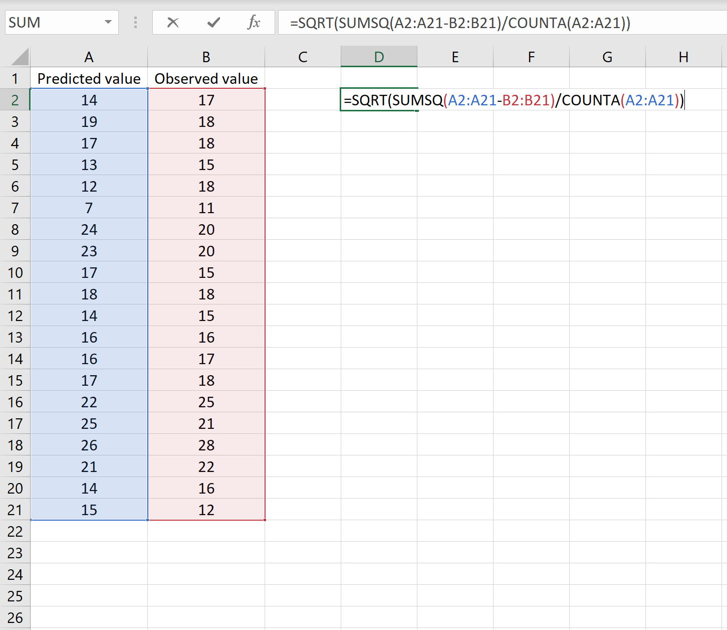
Это говорит нам о том, что среднеквадратическая ошибка равна 2,6646 .
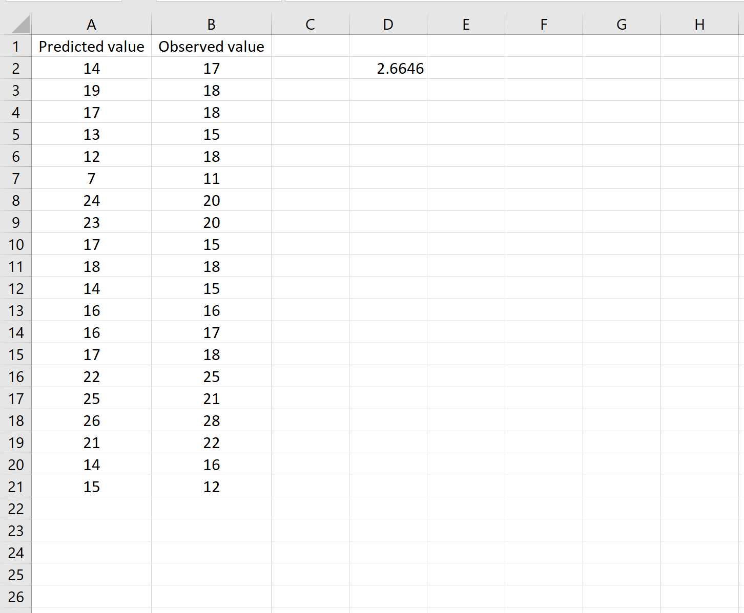
Формула может показаться немного сложной, но она имеет смысл, если ее разобрать:
= КОРЕНЬ( СУММСК(A2:A21-B2:B21) / СЧЕТЧ(A2:A21) )
- Во-первых, мы вычисляем сумму квадратов разностей между прогнозируемыми и наблюдаемыми значениями, используя функцию СУММСК() .
- Затем мы делим на размер выборки набора данных, используя COUNTA() , который подсчитывает количество непустых ячеек в диапазоне.
- Наконец, мы извлекаем квадратный корень из всего вычисления, используя функцию SQRT() .
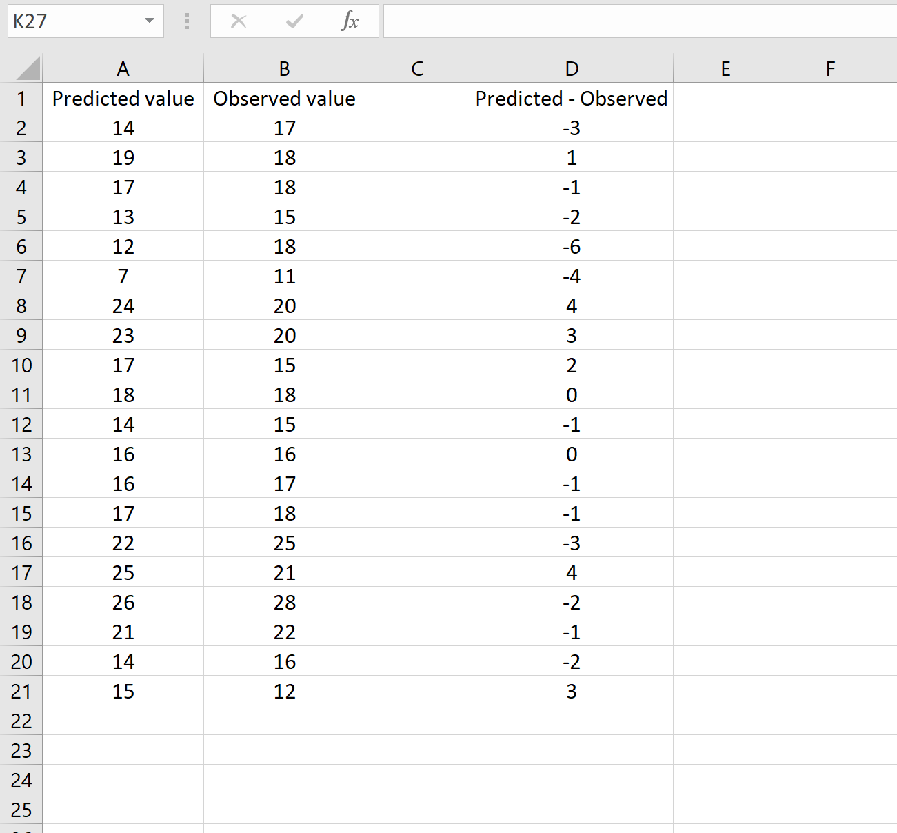
Сценарий 2
В другом сценарии вы, возможно, уже вычислили разницу между прогнозируемыми и наблюдаемыми значениями. В этом случае у вас будет только один столбец, отображающий различия.
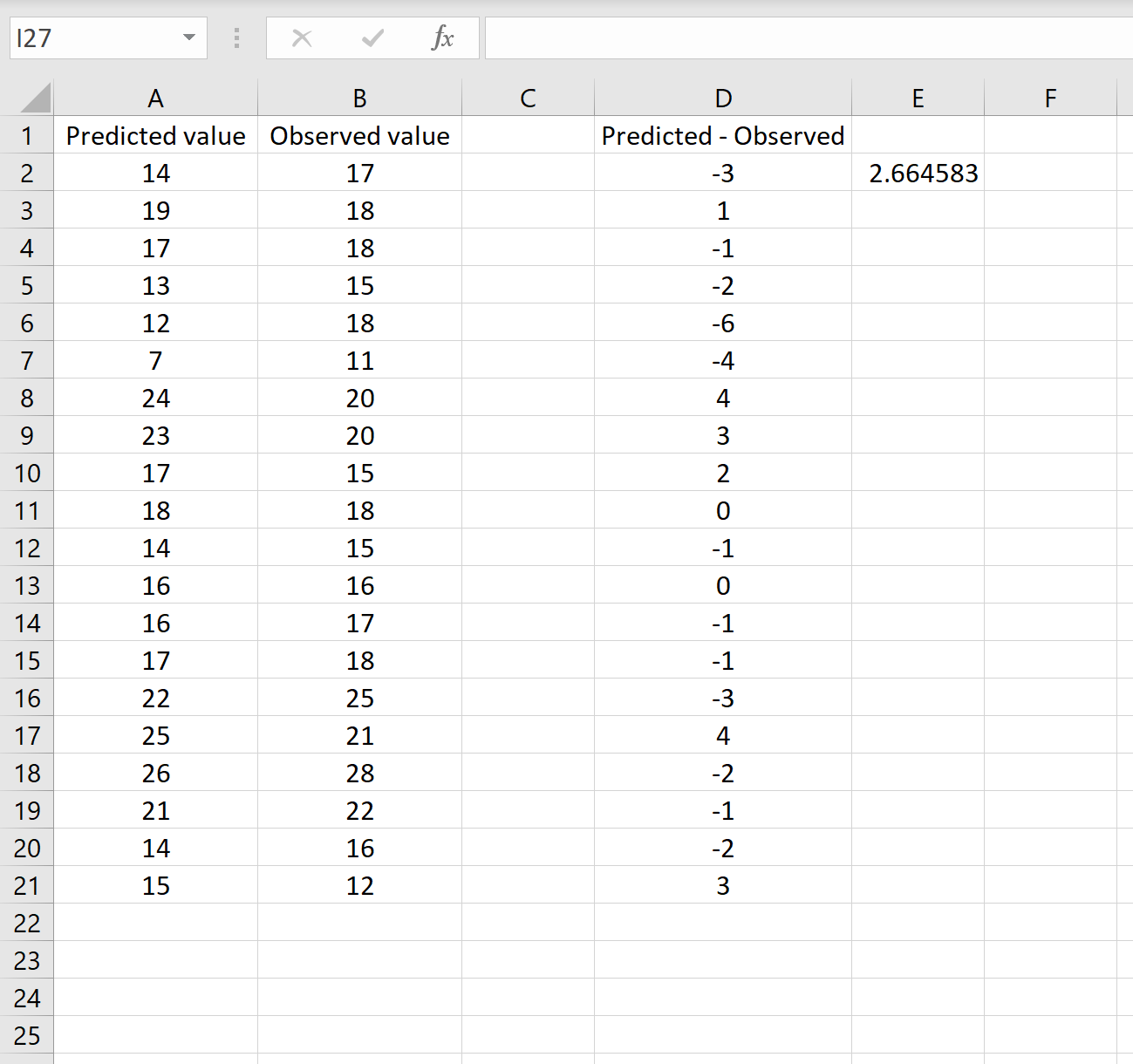
На изображении ниже показан пример этого сценария. Прогнозируемые значения отображаются в столбце A, наблюдаемые значения — в столбце B, а разница между прогнозируемыми и наблюдаемыми значениями — в столбце D:
Если это так, то вы можете рассчитать RMSE, введя следующую формулу в любую ячейку, а затем нажав CTRL+SHIFT+ENTER:
=КОРЕНЬ(СУММСК(D2:D21) / СЧЕТЧ(D2:D21))
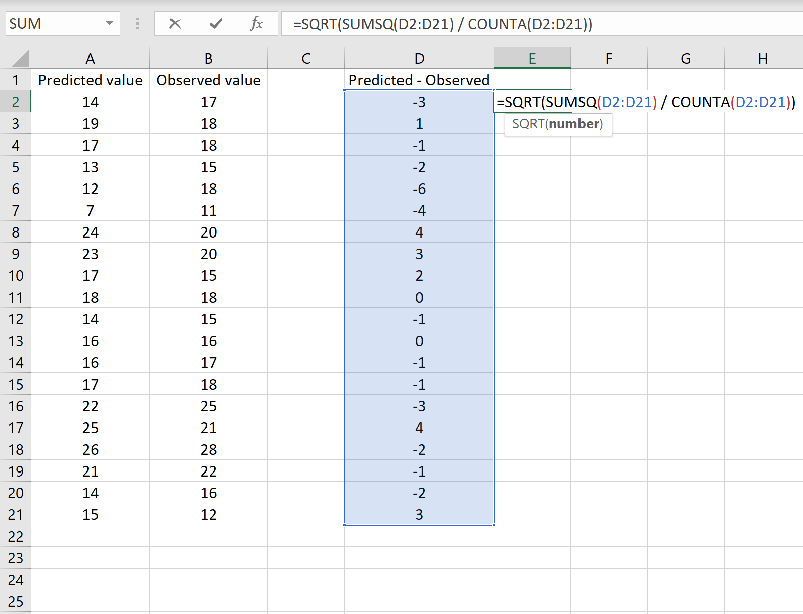
Это говорит нам о том, что среднеквадратическая ошибка равна 2,6646 , что соответствует результату, полученному в первом сценарии. Это подтверждает, что эти два подхода к расчету RMSE эквивалентны.
Формула, которую мы использовали в этом сценарии, лишь немного отличается от той, что мы использовали в предыдущем сценарии:
= КОРЕНЬ (СУММСК(D2 :D21) / СЧЕТЧ(D2:D21) )
- Поскольку мы уже рассчитали разницу между предсказанными и наблюдаемыми значениями в столбце D, мы можем вычислить сумму квадратов разностей с помощью функции СУММСК().только со значениями в столбце D.
- Затем мы делим на размер выборки набора данных, используя COUNTA() , который подсчитывает количество непустых ячеек в диапазоне.
- Наконец, мы извлекаем квадратный корень из всего вычисления, используя функцию SQRT() .
Как интерпретировать среднеквадратичную ошибку
Как упоминалось ранее, RMSE — это полезный способ увидеть, насколько хорошо регрессионная модель (или любая модель, которая выдает прогнозируемые значения) способна «соответствовать» набору данных.
Чем больше RMSE, тем больше разница между прогнозируемыми и наблюдаемыми значениями, а это означает, что модель регрессии хуже соответствует данным. И наоборот, чем меньше RMSE, тем лучше модель соответствует данным.
Может быть особенно полезно сравнить RMSE двух разных моделей друг с другом, чтобы увидеть, какая модель лучше соответствует данным.
Для получения дополнительных руководств по Excel обязательно ознакомьтесь с нашей страницей руководств по Excel , на которой перечислены все учебные пособия Excel по статистике.
Среднеквадратичная ошибка (Mean Squared Error) – Среднее арифметическое (Mean) квадратов разностей между предсказанными и реальными значениями Модели (Model) Машинного обучения (ML):

Рассчитывается с помощью формулы, которая будет пояснена в примере ниже:
$$MSE = frac{1}{n} × sum_{i=1}^n (y_i — widetilde{y}_i)^2$$
$$MSEspace{}{–}space{Среднеквадратическая}space{ошибка,}$$
$$nspace{}{–}space{количество}space{наблюдений,}$$
$$y_ispace{}{–}space{фактическая}space{координата}space{наблюдения,}$$
$$widetilde{y}_ispace{}{–}space{предсказанная}space{координата}space{наблюдения,}$$
MSE практически никогда не равен нулю, и происходит это из-за элемента случайности в данных или неучитывания Оценочной функцией (Estimator) всех факторов, которые могли бы улучшить предсказательную способность.
Пример. Исследуем линейную регрессию, изображенную на графике выше, и установим величину среднеквадратической Ошибки (Error). Фактические координаты точек-Наблюдений (Observation) выглядят следующим образом:

Мы имеем дело с Линейной регрессией (Linear Regression), потому уравнение, предсказывающее положение записей, можно представить с помощью формулы:
$$y = M * x + b$$
$$yspace{–}space{значение}space{координаты}space{оси}space{y,}$$
$$Mspace{–}space{уклон}space{прямой}$$
$$xspace{–}space{значение}space{координаты}space{оси}space{x,}$$
$$bspace{–}space{смещение}space{прямой}space{относительно}space{начала}space{координат}$$
Параметры M и b уравнения нам, к счастью, известны в данном обучающем примере, и потому уравнение выглядит следующим образом:
$$y = 0,5252 * x + 17,306$$
Зная координаты реальных записей и уравнение линейной регрессии, мы можем восстановить полные координаты предсказанных наблюдений, обозначенных серыми точками на графике выше. Простой подстановкой значения координаты x в уравнение мы рассчитаем значение координаты ỹ:

Рассчитаем квадрат разницы между Y и Ỹ:

Сумма таких квадратов равна 4 445. Осталось только разделить это число на количество наблюдений (9):
$$MSE = frac{1}{9} × 4445 = 493$$
Само по себе число в такой ситуации становится показательным, когда Дата-сайентист (Data Scientist) предпринимает попытки улучшить предсказательную способность модели и сравнивает MSE каждой итерации, выбирая такое уравнение, что сгенерирует наименьшую погрешность в предсказаниях.
MSE и Scikit-learn
Среднеквадратическую ошибку можно вычислить с помощью SkLearn. Для начала импортируем функцию:
import sklearn
from sklearn.metrics import mean_squared_error
Инициализируем крошечные списки, содержащие реальные и предсказанные координаты y:
y_true = [5, 41, 70, 77, 134, 68, 138, 101, 131]
y_pred = [23, 35, 55, 90, 93, 103, 118, 121, 129]
Инициируем функцию mean_squared_error(), которая рассчитает MSE тем же способом, что и формула выше:
mean_squared_error(y_true, y_pred)
Интересно, что конечный результат на 3 отличается от расчетов с помощью Apple Numbers:
496.0Ноутбук, не требующий дополнительной настройки на момент написания статьи, можно скачать здесь.
Автор оригинальной статьи: @mmoshikoo
Фото: @tobyelliott
Disease Modelling and Public Health, Part A
Anuj Mubayi, in Handbook of Statistics, 2017
A.5.1 MATLAB® Inbuilt-Function (Classregtree)
To create Regression Trees collect your known input data into a matrix X. Collect the responses to X in a response variable Y and perform following steps.
- •
-
t = classregtree(X, Y, ‘names, ′{‘x1′, ‘x2′, …})
- •
-
treetype = type(t) % tells that it is regression or classification tree
- •
-
view(t) % returns a text description of the tree view(t, ‘mode, ′‘graph′) % returns a graphic description of the tree.
- •
-
qetoler—Defines tolerance on quadratic error per node for regression trees. Splitting nodes stops when quadratic error per node drops below qetoler * qed, where qed is the quadratic error for the entire data computed before the decision tree is grown: qed = norm(y − ybar) with ybar estimated as the average of the input array Y. Default value is 1e − 6.
- •
-
The tree predicts the response values at the circular leaf (terminal) nodes based on a series of questions about the response at the nonterminal branching nodes. A true answer to any question follows the branch to the left; a false follows the branch to the right. For example, we can use the tree to predict the HIV prevalence when the mortality and progression has some fixed value.
predict(tree, [2200, 4, …]) % Predict the response variable when x1 = 2200, x2 = 4, ….
That is, suppose the points (xi, yi), (x2;y2), …, (xc;yc) are all the samples belonging to the leaf-node l. Then our model for l is just ŷ=1c∑i=1cyi, the sample mean of the response variable in that cell. This is a piecewise-constant model.
- •
-
We can use a variety of other methods of the classregtree class, such as cutvar, cuttype, and cutcategories, to get more information about the split at the node 3 (e.g., cutvar(t,3) % what variable determines the split?).
- •
-
cost = test(t, ′resubstitution′) computes the cost of the tree t using a resubstitution method. The cost of the tree is the sum over all terminal nodes of the estimated probability of a node times the cost of a node. If t is a regression tree, the cost of a node is the average squared error over the observations in that node. Cost is a vector of cost values for each subtree in the optimal pruning sequence for t. The resubstitution cost is based on the same sample that was used to create the original tree, so it under estimates the likely cost of applying the tree to new data.
- •
-
To find predictor importance, we use imp = predictorImportance(t)
(provides vector (of length as X) of values with higher value indicates that corresponding independent variable has most impact on the response variable)
- •
-
yfit = eval(t, X) takes a classification or regression tree t and a matrix X of predictors, and produces a vector yfit of predicted response values. For a regression tree, yfit(i) is the fitted response value for a point having the predictor values X(i, :).
Read full chapter
URL:
https://www.sciencedirect.com/science/article/pii/S0169716117300172
Wavelets: Mathematical Theory
K. Schneider, M. Farge, in Encyclopedia of Mathematical Physics, 2006
Wavelet Denoising
We consider a function f which is corrupted by a Gaussian white noise n∈N0,σ2. The noise is spread over all wavelet coefficients s˜λ, while, typically, the original function f is determined by only few significant wavelet coefficients. The aim is then to reconstruct the function f from the observed noisy signal s=f+n.
The principle of the wavelet denoising can be summarized in the following procedure:
- •
-
Decomposition. Compute the wavelet coefficients s˜λ using the FWT.
- •
-
Thresholding. Apply the thresholding function ρɛ to the wavelet coefficients s˜λ, thus reducing the relative importance of the coefficients with small absolute value.
- •
-
Reconstruction. Reconstruct a denoised version sC from the thresholded wavelet coefficients using the fast inverse wavelet transform.
The thresholding parameter ɛ depends on the variance of the noise and on the sample size N. The thresholding function ρ we consider corresponds to hard thresholding:
[66]ρɛ(a)={aif|a|>ɛ0if|a|≤ɛ
Donoho and Johnstone (1994) have shown that there exists an optimal ɛ for which the relative quadratic error between the signal s and its estimator sC is close to the minimax error for all signals s∈H, where H belongs to a wide class of function spaces, including Hölder and Besov spaces. They showed using the threshold
[67]ɛD=σn2lnN
yields an error which is close to the minimum error. The threshold ɛD depends only on the sampling N and on the variance of the noise σn; hence, it is called universal threshold. However, in many applications, σn is unknown and has to be estimated from the available noisy data s. For this, the present authors have developed an iterative algorithm (see Azzolini et al. (2005)), which is sketched in the following:
- 1.
-
Initialization
- (a)
-
given sk,k=0,…,N−1. Set i=0 and compute the FWT of s to obtain s˜λ
- (b)
-
compute the variance σ02 of s as a rough estimate of the variance of n and compute the corresponding threshold ɛ0=2lnNσ021/2;
- (c)
-
set the number of coefficients considered as noise Nnoise=N.
- 2.
-
Main loop repeat
- (a)
-
set Nnoise′=Nnoise and count the wavelet coefficients Nnoise with modulus smaller than ɛi;
- (b)
-
compute the new variance σi+12 from the wavelet coefficients whose modulus is smaller than ɛi and the new threshold ɛi+1=2lnNσi+121/2;
- (c)
-
set i=i+1 until (Nnoise′==Nnoise).
- 3.
-
Final step
- (a)
-
compute sC from the coefficients with modulus larger than ɛi using the inverse FWT.
Example
To illustrate the properties of the denoising algorithm, we apply it to a one-dimensional test signal. We construct a noisy signal s by superposing a Gaussian white noise, with zero mean and variance σW2=1, to a function f, normalized such that ((1/N)∑k|fk|2)1/2=10. The number of samples is N = 8192. Figure 9a shows the function f together with the noise n; Figure 9b shows the constructed noisy signal s and Figure 9c shows the wavelet denoised signal sC together with the extracted noise.

Figure 9. Construction (top) of a 1D noisy signal s=f+n (middle), and results obtained by the recursive denoising algorithm (bottom).
Read full chapter
URL:
https://www.sciencedirect.com/science/article/pii/B012512666200153X
Linear Regression Models
Milan Meloun, Jiří Militký, in Statistical Data Analysis, 2011
6.8 Procedure for Linear Regression Analysis
The procedure for examination and construction of a linear regression model consists of following steps [71,72].
- (1)
-
Proposal of a model
The procedure should always start from the simplest model, with individual independent controllable variables not raised to powers other than the first, and with no interaction terms of the type xjxk included. Only in cases when it is known that the model contains functions of the controllable variables is an exception made.
- (2)
-
Exploratory data analysis in regression
The scatter of individual variables and all possible pair combinations are examined. The scatter plots of xj vs. xk or the index plots xj vs. j are often used here. In this step of a regression analysis, the significance of individual variables with reference to scatter and the presence of multicollinearity is examined. An approximately linear relationship between variables in scatter plots of xj vs. xk indicates multicollinearity. Also, in this step the influential points causing multicollinearity are detected.
- (3)
-
Parameter estimation
The parameters of the proposed regression model and the corresponding basic statistical characteristics of this model are determined by the classical least-squares method (LS). Individual parameters are tested for significance by using the Student t-test, the determination coefficient R^2 and the predicted determination coefficient R^P2. Other statistical characteristics calculated are the total F-test, the model significance test, the model complexity test, the mean quadratic error of prediction MEP and the Akaike information criterion AIC, to examine the linearity of model.
- (4)
-
Analysis of regression diagnostics
The statistical analysis of classical residuals leads to estimates of residual variance σ^2e^, residual standard deviation Se^, residual skewness g^1e^, residual kurtosis g^2e^, the Pearson χ2-test of residual normality and the Jarque-Berra normality test. Different diagnostic graphs are used to examine the regression diagnostics for identification of influential points, and to test the conditions for the least-squares method, namely homoscedasticity, absence of autocorrelation, and normality of error distribution. If influential points are found, it has to be decided whether these points should be eliminated from data. If points are eliminated, the whole data treatment must be repeated. When there are several controllable variables, the significance of each variable and its function is examined by partial-regression graphs and by the partial-residual graph.
- (5)
-
Construction of a more accurate model
According to the test for fulfilment of the conditions for the least-squares method, and the result of regression diagnostics, a more accurate regression model is constructed as follows.
- (a)
-
When heteroscedasticity is found in the data, the weighted least-squares method (WLS) is used.
- (b)
-
When autocorrelation is found in the data, the generalized least-squares method (GLS) is used.
- (c)
-
When some restrictions apply to the parameters, the conditioned least-squares method (CLS) is used.
- (d)
-
When multicollinearity is found in the data, the method of rational ranks (MRV) is used.
- (e)
-
When all variables are subject to random errors, the extended least-squares method (ELS) is used.
- (f)
-
When the data have an error distribution other than normal, or the data contain outliers or high leverage points, some robust methods are used.
- (6)
-
Evaluation of the quality of the model proposed
With the use of classical tests, regression diagnostics and some supplementary information about the “model + data + method”, the quality of the proposed linear regression model is evaluated.
- (7)
-
Analysis of calibration models
For a calibration model proposed for the given signal value y
*,the quality of the independent variable x
* together with its confidence interval is estimated. Before application of the calibration model, the detection limit and the determination limit should be estimated. These limits determine the allowable lower limit of the calibration model. - (8)
-
Statistical hypothesis testing
In some cases, to compare several straight lines, statistical hypothesis testing is performed.
Read full chapter
URL:
https://www.sciencedirect.com/science/article/pii/B9780857091093500066
Advances in Imaging and electron Physics
O. Losson, … Y. Yang, in Advances in Imaging and Electron Physics, 2010
4.3.1 Fidelity Criteria
These criteria use colors coded in the RGB acquisition color space to estimate the fidelity of the demosaiced image compared with the original image.
- 1
-
Mean Absolute Error
This criterion evaluates the mean absolute error between the original image I and the demosaiced image Î. Denoted by MAE, it is expressed as follows (Chen et al., 2008; Li and Randhawa, 2005):
(82)MAE(I,Iˆ)=13XY∑k=R,G,B∑x=0X−1∑y=0Y−1|Ix,yk−Iˆx,yk|,
where Ix,yk is the level of the color component k at the pixel whose spatial coordinates are (x,y) in the image I. X and Y are, respectively, the number of columns and rows of the image.
The MAE criterion can be used to measure the estimation errors of a specific color component. For example, this criterion is evaluated on the red color plane as
(83)MAER(I,Iˆ)=1XY∑x=0X−1∑y=0Y−1|Ix,yR−Iˆx,yR|.
MAE values range from 0 to 255, and the lower MAE value, the better demosaicing quality.
- 2
-
Mean Square Error
This criterion measures the mean quadratic error between the original image and the demosaiced image. Denoted by MSE, it is defined as follows (Alleysson et al., 2005):
(84)MSE(I,Iˆ)=13XY∑k=R,G,B∑x=0X−1∑y=0Y−1(Ix,yk−Iˆx,yk)2.
The MSE criterion can also measure the error on each color plane, as in Eq. (23). The optimal quality of demosaicing is reached when MSE is equal to 0, whereas the worst is measured when MSE is close to 2552.
- 3
-
Peak Signal-to-Noise Ratio
The PSNR criterion is a widely used distortion measurement to estimate the quality of image compression. Many authors (e.g., Alleysson et al., 2005; Hirakawa and Parks, 2005; Lian et al., 2007; Wu and Zhang, 2004) use this criterion to quantify the performance reached by demosaicing schemes. The PSNR is expressed in decibels as
(85)PSNR(I,Iˆ)=10⋅log10(d2MSE(I,Iˆ)),
where d is the maximum color component level. When the color components are quantized with 8 bits, d is set to 255.
Like the preceding criteria, PSNR can be applied to a specific color plane. For the red color component, it is defined as
(86)PSNRR(I,Iˆ)=10⋅log10(d2MSER(I,Iˆ)).
The higher the PSNR value, the better the demosaicing quality. The PSNR measured on demosaiced images generally ranges from 30 to 40 dB (i.e., MSE ranges from 65.03 to 6.50).
- 4
-
Correlation
A correlation measurement between the original image and the demosaiced image is used by Su and Willis (2003) to quantify the demosaicing performance. The correlation criterion between two grey-level images I and Î is expressed as
(87)C(I,Iˆ)=|(∑x=0X−1∑y=0Y−1Ix,yIˆx,y)−XYμμˆ[(∑x=0X−1∑y=0Y−1Ix,y2)−XYμ2]1/2[(∑x=0X−1∑y=0Y−1Iˆx,y2)−XYμˆ2]1/2|,
where μ and μˆ are the mean grey levels in the two images.
When a color demosaiced image is considered, the correlation level Ck (Ik,Îk), k ∈ {R,G,B} between the original and demosaiced color planes is estimated. The mean of the three correlation levels is used to measure the quality of demosaicing. The correlation levels C range between 0 and 1, and a measurement close to 1 can be considered a satisfying demosaicing quality.
Read full chapter
URL:
https://www.sciencedirect.com/science/article/pii/S1076567010620058
Characterisation of Porous Solids V
Joachim Gross, in Studies in Surface Science and Catalysis, 2000
Discussion
Theoretically, the permeability should vary with pressure according to [11]
(1)d=d∞1+μp.
Here, d∞ is the permeability for liquids (at „infinite” pressure) and μ is the crossover pressure between molecular flow (at low pressure) and viscous flow in the pores. In fig. 6 the permeability is plotted as function of 1/p. The axis section of a straight line fit to the data should give d∞ and the slope is μ d∞. The crossover from molecular flow to viscous floyd is the pressure at which the gas molecules start colliding with each other more frequently than with the pore walls; thus, the mean free path p = μ is equal to a mean pore size R [12]:

Fig. 6. The permeability for all steps up to crack formation, plotted as function of inverse pressure, 1/p. The straight line is a fit for the inverse pressure range 0.22… 4 MPa− 1.
(2)μ=1R32η3π2πR0TM,
where η is the viscosity of the gas (15 μPa s for CO2 at 45 °C), M its molecular weight, T the temperature and R0 the gas constant. Since all of the gas properties are known. R can be calculated from the fit value of μ. For the fit data in the straight part of Fig. 6 are used that yield the lowest quadratic error per data point. In table 1 the values found for parameters extracted from the dynamic pressurization experiment are compared to those obtained from other methods. In case of the mean pore size. this is the mean chord length within the pores, which can be calculated from the relative density:
Table 1. Comparison of aerogel properties from dynamic pressurization with independently acquired data
| parameter from dynamic pressurization | value | comparable value | source of comparable value |
|---|---|---|---|
| d∞ | 17 nm2 | 13 nm2 | permeability from beam bending experiment in ethanol |
| breakthrough radius rBT | 14 nm | 12 nm | from permeability |
| bulk modulus K at p = 0 | 3.0 MPa | 3.0 MPa 1.0 MPa | sound velocity beam bending (wet gel) |
| pore diameter R, derived from μ | 30 ± 3 nm | 30 ± 8 nm | mean pore size. from density and surface area |
(3)R=43Rsρ1–ρ
The particle size Rs can be estimated using the skeletal density of sol-gel silica (ρs = 2000 kgm− 3) and a typical specific surface area of S = 600 m2 g− 1 to be of the order of 2.5 nm. The result shown for R in table 1 depends quite sensitively on the parameters used to calculate it, so it is not expected to be very accurate (30% at best), but it compares very well to the one from the DP experiment.
The permeability at infinite pressure d∞ (l/p = 0) is comparable to the value measured by beam bending for ethanol. Despite of the sample shrinkage during supercritical drying it is actually slightly larger (table 1), however the agreement is still satisfactory. From the permeability, the breakthrough radius rBT can be calculated [13], a pore size governing fluid flow through the aerogel pores. As seen in table 1, the result is much smaller than R calculated from μ. This is expected since the interconnections of pores are usually smaller than the average free pore space.
The bulk modulus plotted in fig. 4 should be pressure independent. While there is perfect agreement at low pressure, above 7 MPa it sharply increases and is not compatible any more with the value found from the sound velocity. A possible reason could be temperature gradients in the autoclave, which would cause a variation of the gas properties that enter the parameter calculation. It was tried to recalculate all parameters assuming up to 3 °C temperature deviation. The resulting parameter variation is smaller than the symbol size in fig 4 in the plateau region (0.2 to 7 MPa), but even outside that area the deviations are too small to explain the huge bulk moduli at high pressures. Another possibility is an uncertainty in the compressibility of the gas. Due to quick pressure changes, the gas — skeleton composite behaves adiabatic rather than isothermal [4]. This is accounted for in the theory. However, since the pressure relaxation takes several seconds, a partial thermal relaxation might take place as well. Comparing the thermal diffusivity of CO2 with the gas diffusion constant derived from the permeability shows, however, that the latter is about one order of magnitude higher, so thermal relaxation of the sample should be slow compared to the pressure relaxation. As an alternative explanation we offer the fact that the vicinity of the critical point of CO2 produces considerable uncertainty in the gas properties. As a consequence, we consider all data above about 7 MPa as inaccurate. Fortunately, for the permeability analysis presented above only pressures in the vicinity of μ are significant, so the pressure range for accurate data is clearly sufficient. The bulk modulus derived from the beam bending experiments in table 1 is only given for reference. It is known that during the supercritical drying process the modulus of gels rises considerably, even when the gentle CO2 drying is employed [14].
To our knowledge, this study is the first to observe a reversible dimensional change of aerogels with gas pressure. We should note that, in fact, most of the shrinkage observed for CO2 dried aerogels occurs during depressurization. We do not yet have a definite explanation for this effect. It appears to be rather complex, as suggested by the varying slope in fig. 5. A possible cause is a change of van-der-Waals interactions of skeletal elements of the aerogel across a gas medium of varying density. Another possibility would be the presence of a surface layer of ethanol, which changes its surface tension with CO2 pressure. In a different aerogel system, shrinkage during CO2 drying was attributed to a change in the Zeta potential [15], which reflects the surface charge density. This appears to be possibility for our silica aerogel as well. Further experiments are probably necessary to shed more light on this fascinating new aspect of highly porous materials.
Read full chapter
URL:
https://www.sciencedirect.com/science/article/pii/S0167299100800725
Derivative: tool for approximation and investigation
Petr Habala, in Calculus for Engineering Students, 2020
Answers to exercises
2.3.1.1: Setup: radius r(t), volume V(t), given V′, and we need to know r′.
Connection: V=43πr3. Then V′=4πr2r′, and hence r′=V′4πr2. If we blow at a constant rate, then the radius of the balloon grows at the rate r′=Kr2.
2.3.1.2: Setup: position x(t) (in meters), distance d(t), known x′(t), and we need d′(t).

The relation we seek is d=22+x2. Taking derivative (and canceling 2) we obtain d′=x22+x2x′. Note that there is a difference between velocity, speed, and rate of change. In particular, if the car goes towards the radar, then d′ is negative, while the speed of the car should be positive. We therefore introduce vC for the true speed and vA for apparent speed of the car and obtain the formula vA=|x|22+x2vC.
Now we look at this formula. First, note that 4+x2>|x|, so the factor |x|4+x2 is always less than 1. In other words, the radar always shows less than the actual speed of the car. When the car is closest to the radar (x=0), the apparent velocity is zero. On the other hand, when the car is really far away (x≈∞), then |x|4+x2≈|x|x2=1. Thus the radar almost shows the actual velocity, which makes sense; the car is then approaching almost head on.
2.3.1.3: Setup: shadow length l(t), distance from lamppost d(t), we know d′, and we want to know l′.

Relation: From similarity of triangles we get l3=l+d6. Hence l=d, that is, l′=d′=c by assumption of steady walk.
Surprisingly enough, my shadow grows at a rate that does not depend on my distance from the lamppost, just on the speed at which I walk. I actually expected that the further I am, the faster the shadow grows, but my intuition was wrong this time.
2.3.2.1: (a) f′(a)≈f(a)−f(a−h)h.
(b) E≈12f″(a)h. The error is linear and should be comparable to that of forward difference.
(c) In Maple I used the following code for the default example f(x)=ex, a=0:

2.3.2.2: (a) f′(a)≈f(a+h)−f(a−h)2h.

(b) E≈−13!f‴(a)h2. Quadratic error disappears much faster than linear error, so this approximation is much more effective than forward or backward difference. In particular, we can get very precise approximations while h is still relatively large, before the numerical errors kick in. But again, if we overdo it, they will show up eventually.
(c) In Maple we can use the following modification of the above code:
![]()
2.3.3.1: (a) Choice a=1, find T4, the others are obtained by truncating it. We have T4(x)=1+1211(x−1)−1214113(x−1)2+1638115(x−1)3−1241516117(x−1)4.
T4(x)=1+12(x−1)−18(x−1)2+116(x−1)3−5128(x−1)4.
Alternative: T4(1+h)=1+12h−18h2+116h3−5128h4.
Approximations:
T2(1.2)=1+12⋅0.2−18(0.2)2=1+110−1200=1+110−51000=1.095,
T3(1.2)=1+12⋅0.2−18(0.2)2+116(0.2)3=1+110−1200+12000=1.0955,
T4(1.2)=1+12⋅0.2−18(0.2)2+116(0.2)3−5128(0.2)4=1.0954375.
(b) Lagrange form of the remainder: E2(1.2)≤13!max|−38c−5/2|⋅(0.2)3,
E3(1.2)≤14!max|1516c−7/2|⋅(0.2)4, E4(1.2)≤15!max|−10532c−9/2|⋅(0.2)5.
Since negative powers of c are decreasing for 1≤c≤1.2, we can estimate
|E2(1.2)|≤13!38⋅153=12000=0.0005,
|E3(1.2)|≤14!1516⋅154=116000=0.0000625,
|E4(1.2)|≤15!10532⋅155=7800000=0.00000875.
Just to satisfy our curiosity, actual errors are E2≈0.0004, E3≈−0.00005, and E4≈0.000008. It seems that the Lagrange estimates are very good here.
2.3.3.2: (a) Choose a=0, f(x)=ln(1+x), then f(n)=(−1)n+1(n−1)!(x+1)n for n≥1 (by induction). Therefore
Tn(x)=0+∑k=1n1k!(−1)k+1(k−1)!1kxk=∑k=1n(−1)k+11kxk.
(b) Lagrange estimate:
En(x)=1(n+1)!(−1)n+2n!(c+1)n+1xn+1=(−1)n1n+11(c+1)n+1xn+1.
We have c between 0 and x and |x|≤0.5, so definitely |c|≤0.5 as well. Since 1(c+1)n+1 is decreasing and positive on this range, we can estimate
|En(x)|≤1n+11(0.5)n+1⋅(0.5)n+1=1n+1=en.
(c) We have en≤10−6⇒n+1≥106, so we take n=106.
The corresponding Tn is a very long polynomial and it would take a long time to evaluate. In fact here the actual error is much smaller, so the error estimate is extremely bad, but the Lagrange form does not allow for a better one. The main problem is the term 1(c+1)n+1. If we restricted our attention to x≥0, then c∈[0,0.5] and we get |En(x)|≤1n+111n+1(0.5)n+1=12n+1(n+1), which tends to zero very fast.
2.3.3.3: (a) Choose a=0, f(x)=sin(x), all derivatives are sines or cosines with plus/minus: f′=cos(x), f″=−sin(x), f‴=−cos(x), f⁗=sin(x), f′′′′′=cos(x), etc. Therefore
Tn(x)=0+x−0−13!x3−0+15!x5+0−17!x7−⋯=x−13!x3+15!x5−17!x7+⋯.
(b) Lagrange estimate: En(x)=1(n+1)!f(n+1)(c)xn+1. The derivative is sines and cosines with alternating signs, but it is never more than 1. Thus, using |x|≤1, we get
|En(x)|≤1(n+1)!⋅1⋅1n+1=1(n+1)!=en.
(c) Since [−π4,π4]⊆[−1,1], we can use the above estimate. We want en≤10−3, and this needs (n+1)!≥1000. By experimentation, n=6 is enough.
2.3.4.1: (a) Ep=U(R+h)−U(R)=−mgR2R+h+mgR2R.
(b) 1r=1R−1R2(r−R)+1R3(r−R)2−1R4(r−R)3+⋯, so 1r≈1R−1R2(r−R).
Thus U(R+h)≈−mg(R−h).
Alternative: 1R+h=1R−1R2h+1R3h2−1R4h3+⋯, so 1R+h≈1R−1R2h.
Bonus question: We can use the formula for summing up geometric series:
1R+h=1R11−(−hR)=1R⋅(1+(−hR)+(−hR)2+(−hR)3+⋯).
Now we see why we can ignore higher powers when h is negligible compared to R, since then the higher powers of the very small number −rR go to zero fast.
Another possibility is to apply the binomial formula to (R+h)−1, but that requires more work.
(c) Ep=U(R+h)−U(R)≈−mgR2(1R−hR2)+mgR2R=mgh.
We obtained the formula for potential energy that we all remember from elementary school. Now we see that it is actually just an approximation of a more precise formula, and that it is valid only for relatively small values of h.
2.3.4.2: (a) T4=12t2+14!⋅9t4=12t2+38t4.
(b) For t small we can approximate γ−1≈12(vc)2, so we get
EK=12v2c2mc2=12mv2.
Note: Instead of using the Taylor polynomial, one can apply the binomial theorem to (1−t2)−1/2.
2.3.5.1: (a) y′(0)=10+1=1, so limx→0+(y(x)−y(0)x)=1. Choosing, ε=1 we obtain δ>0 such that y(x)−y(0)x>1−ε=0 on (0,δ). Since x>0 there, we get y(x)−y(0)>0 and y(0)=0.
(b, c) Similar to the first example.
(d) y″=−1(y+1)2y′<0.
(e) We know that y′>0 on [0,∞) and it is a decreasing function there (since [y′]′=y″<0), and therefore it must have a proper limit L that satisfies L≥0.
Another argument: We know that y→l, where l>0. Then lim(y′)=lim(1y+1)=1l+1=L. Since l>0, this cannot be infinity. Since l=∞ is possible, L can be zero.
(f) Case L>0: Using the definition of the limit with ε=12L we find some K>0 so that y′≥L−ε=12L>0 on [K,∞). By Lemma 2.7 it follows that y(x)→∞ at infinity.
Case L=0: By the given ODE, 1y(x)+1→0 at infinity. This is possible only if y(x)→∞ there.
(g) Since y(x)→∞, L’Hôpital’s rule can be used:
limx→∞(y(x)x)=limx→∞(y′(x)1)=limx→∞(1y(x)+1)=1∞+1=0.
2.3.5.2: (a, b) Similar to the first example.
(c) y″=1(y+1)2y′>0.
(d) It follows by Lemma 2.6 from the fact that y is increasing and concave up on [0,∞).
(e) Since y(x)→∞ at infinity, we can use L’Hôpital’s rule in evaluating limx→∞(y(x)x)=limx→∞(y′(x)1)=limx→∞(y(x)y(x)+1)=limx→∞(11+1/y(x))=11+0=1. This proves the claim.
2.3.5.3: Solution combines approaches from previous exercises.
(c) y″=−1(xy+1)2(y+xy′)<0.
(d) We have limx→∞(y′(x))=limx→∞(1xy(x)+1)=1∞⋅L+1 by (b).
Since L⋅∞=∞ is true for both L>0 and L=∞, we get 1∞⋅L+1=1∞=0.
(e) Case L proper: Then limx→∞(y(x)x) is of the type L∞=0.
Case L=∞: L’Hôpital’s rule can be used:
limx→∞(y(x)x)=limx→∞(y′(x)1)=0 by part (d).
(f) Before, the only way to conclude 1y(x)+1→1L+1=0 was to have L=∞.
Now we have 1xy(x)+1→1∞⋅L+1=0 and this is true also for L that is not infinity.
Read full chapter
URL:
https://www.sciencedirect.com/science/article/pii/B9780128172100000096
Quantum Control of Optomechanical Systems
Sebastian G. Hofer, Klemens Hammerer, in Advances In Atomic, Molecular, and Optical Physics, 2017
B.1.2.2 Characteristic Function Technique
Suppose we continuously monitor the output of a quantum system whose evolution is described by Eq. (A.11) via homodyne detection, yielding a measurement of the field quadrature Y(t)=Aout(t)+Aout†(t) [where Aout is defined in (A.25)]. We denote by Yt={Y(t′):0≤t′≤t} the algebra generated by the observation process Y and by Yt′ its commutant, Yt′={A:[A,Y]=0,∀Y∈Yt}. For 0 ≤ t′≤ t we then have the nondemolition property (Bouten et al., 2007)
(B.22)[jt(X),Y(t′)]=0
[such that jt(X)∈Yt] and the self-nondemolition property
(B.23)[Y(t),Y(t′)]=0.
This allows us to map the quantum filtering problem to a classical filtering problem which we can tackle by methods from classical nonlinear filtering theory.
We define the quantum state E[⋅]=tr(ρ0⊗ρvac⋅) and seek to find an estimate πt(X)∈Yt for the Heisenberg operator X(t) = jt(X) which minimizes the quadratic error E[(πt(X)−jt(X))2] based on the observations Y (t). As this requirement is equivalent to Eq. (B.21) we directly find
(B.24)πt(X)=E[jt(X)|Yt].
We will now show how to calculate πt(X) explicitly using the characteristic function technique (Gough and Kostler, 2010), for the case of a single vacuum input. Due to the orthogonality property (B.20) of the conditional expectation we have the identity E[(πt(X)−jt(X))Ct]=0 for all Ct∈Yt. We can thus make the following Ansatz
(B.25a)dCt=gtCtdY(t),
(B.25b)dπt(X)=αtdt+βtdY(t),
for adapted stochastic processes αt,βt∈Yt. This implies Ct,πt(X)∈Yt [while on the other hand jt(X)∉Yt]. We can then use dE[(πt(X)−jt(X))Ct]=0, which, due to Itō-rules consists of three terms. We find for the first term
I=E[(dπt(X)−djt(X))Ct]=E[αtCt]dt+E[βtdY(t)Ct]−E[djt(X)Ct]=E[αtCt]dt+E[βtjt(s+s†)Ct]dt−E[jt(L*X)Ct]dt=E[αtCt]dt+E[βtπt(s+s†)Ct]dt−E[πt(L*X)Ct]dt,
where to go from the second to the third line we used (i) the fact that Y is generated by a Wiener process and therefore the increments dY (t) are independent of Y (t) at equal times, i.e., E[dY(t)f(Y(t))]=E[E[dY(t)]f(Y(t))] for a measureable function f, (ii) E[dY(t)]=E[jt(s+s†)]dt, and (iii) for the field initially in vacuum we have E[dA(t)]=0 and E[dA†(t)]=0. In particular this means that E[βtdA(t)Ct]=E[βtdA†(t)Ct]=0. To go to the fourth line we used the orthogonality property, thus E[jt(X)Ct]=E[πt(X)Ct]. For the second term we find
II=E[(πt(X)−jt(X))dCt]=E[(πt(X)−jt(X))gtCtjt(s+s†)]dt=E[πt(X)πt(s+s†)gtCt]dt−E[πt(X(s+s†))gtCt]dt
by the same reasoning as above. Going from the second to the third line we used (B.19c), which implies πt(πt(X)jt(s)) = πt(X)πt(s), and jt(XY ) = jt(X)jt(Y ). For the third term we obtain by using the Itō table (A.14)
III=E[(dπt(X)−djt(X))dCt]=E[(βt(X)dY(t)−djt(X))gtCtdY(t)]=E[βt(X)gtCt]dt−E[jt([s†,X])gtCt]dt=E[βt(X)gtCt]dt−E[πt([s†,X])gtCt]dt.
As gt is an arbitrary function we can deduce from I + II + III = 0 by equating the coefficients of gt and gtCt that
0=αt+βtπt(s+s†)−πt(L*X),0=πt(X)πt(s+s†)−πt(X(s+s†))+βt−πt([s†,X])=πt(X)πt(s+s†)−πt(Xs+s†X)+βt,
where both equalities hold almost surely with respect to E. Solving this for αt and βt, and using the ansatz (B.25b) we find for the quantum filter
(B.26)dπt(X)=πt(L*X)dt+[πt(Xs+s†X)−πt(X)πt(s+s†)]dW,
where
(B.27)dW(t)=dY(t)−πt(s+s†)dt
is the innovations process. W(t) is a Wiener process with E[dW]=0, dW2 = dt and therefore E[πs(X)dW(t)]=0 for 0 ≤ s ≤ t. The innovations process can be interpreted as the difference between the observed changed dY (t) and the expected change πt(s + s†)dt of the field. We can obtain the adjoint equation for the conditional density matrix ρc by identifying πt(X) = tr(ρc(t)X). This leads to the SME (B.8).
Read full chapter
URL:
https://www.sciencedirect.com/science/article/pii/S1049250X17300149
Goodness-of-fit test for interest rate models: An approach based on empirical processes
Abelardo Monsalve-Cobis, … Manuel Febrero-Bande, in Computational Statistics & Data Analysis, 2011
1 Introduction
In finance, continuous time models, particularly diffusion processes, are frequently used to characterise the dynamics of major economic variables such as exchange rates, asset valuations and interest rates. One model frequently used to characterise the dynamics of interest rates is the diffusion model in continuous time, also known as the Itô process, which is given by the stochastic differential equation,
(1)drt=μ(rt)dt+σ(rt)dWt,
where Wt is standard Brownian motion, and μ(rt) and σ(rt) are called the drift function and the diffusion (or volatility function), respectively. Parametric models are often useful to finance professionals because observations can be interpreted in terms of parameters. A parametric representation of Model (1) is given by
(2)drt=μ(rt,θ)dt+σ(rt,θ)dWt,
where θ is a d-dimensional unknown parameter within a parameter space Θ⊂Rd for some positive integer d. In the market, models are continuously refined, and their ability to fit current prices is continuously tested. Models are less frequently tested for their goodness of fit to historical data. Research in this context has exhibited notable growth and development, but no definitive model has yet been produced. For this reason, one of the main goals of this work is to apply our goodness of fit approach to the diffusion processes that are studied in the literature for modelling interest rates.
The properties of interest rate processes are determined completely by the drift and volatility functions. Consequently, the problem of selecting among the models in the literature, or possibly determining that none are suitable, reduces to choosing or estimating the drift and volatility functions. Because there may be a number of competing models, every statistical inference that is based on a particular model should be accompanied by a proper model check to prevent erroneous conclusions. Recent studies on the specification of continuous time diffusion processes include Aït-Sahalia (1996), Gao and King (2004), Hong and Li (2005) and Chen et al. (2008), who propose tests to compare the parametric specifications of a diffusion process using the marginal or transition density functions of the process; Corradi and White (1999), who present a normal asymptotic test for the diffusion function; Dette and von Lieres und Wilkau (2003), who propose a test for parametric forms of the volatility function based on the stochastic integrated volatility process; Li (2007), who proposes a nonparametric test for parametric specifications of the diffusion function that is based on the quadratic error between the estimated nonparametric diffusion function and the diffusion proposed under the null hypothesis; Arapis and Gao (2006) and Gao and Casas (2008), who propose a test to determine parametric forms of the drift and volatility functions based on smoothing techniques; Fan and Zhang (2003) and Fan et al. (2003), who propose simultaneous tests for the specifications of the drift and diffusion functions based on a likelihood ratio test; and Aït-Sahalia et al. (2010), who propose a test based on the Chapman–Kolmogorov equation. The proposals mentioned above, in most cases, are based on using smoothing techniques, for the estimation of a model or proposed test. This kind of methodology represents an additional disadvantage as the selection of the smoothing parameter can also affect the power of the test.
In this paper, we consider a goodness-of-fit test based on empirical processes such as model checks. The aim is to introduce a test that compares the goodness of fit for parametric forms of the drift and volatility functions in interest rate models based on empirical processes. The hypotheses being studied are
(3)H0:μ∈{μ(⋅,θ):θ∈Θ}
for the parametric form of the drift, and
(4)H0:σ∈{σ(⋅,θ):θ∈Θ}
for the parametric form of the volatility function. An alternative way to address the problem would be to use the proposed tests for the integrated regression models. In regression models, this approach is discussed in Stute (1997), and a similar approach is later considered for time series in Koul and Stute (1999). The literature on the goodness of fit of diffusion models based on empirical processes, is scarce, with the exception of the some recent works: Lee and Wee (2008), who propose a test based on the empirical process of the residues of the diffusion model; and Negri and Nishiyama (2009), Negri and Nishiyama (2010) and Masuda et al. (2010), who propose a goodness-of-fit test based on a score-marked empirical process for both continuous and discrete time observations of ergodic diffusion processes. The above works only consider tests of a simple null hypothesis. In this sense, our proposal addresses a more general case: the composite hypothesis for a parametric form of the drift function. We also propose a test for the volatility function based on empirical processes that have not been considered in previous works.
This paper proposes using a goodness-of-fit test that can be implemented easily and efficiently by rewriting the diffusion process as a regression or time series model. Then, the goodness-of-fit test for the drift function can be derived from the integrated regression function of the process variations that characterise the interest rates, producing an empirical process based on the residuals. The test for the volatility function is constructed from the integrated conditional variance function, which gives a new empirical process that can be compared with the hypothesis of a parametric form of the volatility function. The distributions of both statistics are approximated using bootstrap techniques as observed in the regression models presented in Stute et al. (1998). Note that implementing the test requires only estimating the parameters of the process (using consistent “root—n” estimators) and applying a bootstrap procedure. These steps will be described in detail later in discussions regarding the calibration of the test statistic distribution, which is found to be relatively simple.
The article is structured as follows. Section 2 presents the diffusion model on which the study will be based. In Section 3, the construction of goodness-of-fit tests for the drift function and the volatility function will be presented. Some issues related to the consistency of the bootstrap resampling and the drift function test are discussed. In Section 4, a simulation study of the proposed tests will be implemented, and the level and power of the tests will be verified. In addition, a particular extension of the test for jump diffusion processes is introduced. Finally, Section 5 will present an application of the model to the series of EURIBOR interest rates.
Read full article
URL:
https://www.sciencedirect.com/science/article/pii/S0167947311002052
Machines learn by means of a loss function which reflects how well a specific model performs with the given data. If predictions deviate too much from actual results, loss function would yield a very large value. Gradually, with  function, parameters are modified accordingly to reduce the error in prediction. In this article, we will quickly review some common loss functions and their usage in the domain of machine/deep learning.
Unfortunately, there’s no one-size-fits-all loss function to algorithms in machine learning. There are various factors involved in choosing a loss function for a specific problem such as type of machine learning algorithm chosen, ease of calculating the derivatives and to some degree the percentage of outliers in the data set.
As we have two common problems, classification and regression, loss functions also can be sorted into two major categories — Classification losses and Regression losses.
NOTE
n - Number of training examples.
i - ith training example in a data set.
y(i)- Ground truth label for ith training example.
y_hat(i) - Prediction for ith training example.
Contents
- 1 Classification Losses
- 1.1 Zero-one loss
- 1.2 Hinge Loss/Multi-class SVM Loss
- 1.3 Cross-Entropy Loss/Negative Log-Likelihood
- 2 Regression Losses
- 2.1 Mean Square Error/Quadratic Loss/L2 Loss
- 2.2 Mean Absolute Error/L1 Loss
- 2.3 Mean Bias Error
- 3 Wrapping up
- 3.1 Share this:
Classification Losses
In classification, we are trying to predict the output from a set of finite categorical values, e.g. given large data set of images of handwritten digits, categorizing them into one of 0–9 digits.

Zero-one loss
In statistics and decision theory, a frequently used loss function is the 0-1 loss function
![[L({hat {y}},y)=I({hat {y}}neq y),,]](https://i0.wp.com/petamind.com/wp-content/ql-cache/quicklatex.com-de3227821785d705e54c261cbebd6a31_l3.png?resize=146%2C19&ssl=1 "Rendered by QuickLaTeX.com")
where I is the indicator function. The function is non-continuous and thus impractical to optimize.
from sklearn.metrics import zero_one_loss
y_pred = [1, 2, 3, 4]
y_true = [2, 2, 9, 4]
zero_one_loss(y_true, y_pred)
L = zero_one_loss(y_true, y_pred, normalize=False)
#L = 2 as there is two place difference
Hinge Loss/Multi-class SVM Loss
In simple terms, the score of the correct category should be greater than the sum of scores of all incorrect categories by some safety margin (usually one). And hence hinge loss is used for maximum-margin classification, most notably for support vector machines. Although not differentiable, it’s a convex function which makes it easy to work with usual convex optimizers used in the machine learning domain.
Mathematical formulation:
![[SVMloss = sumlimits_{j # y_i} max(0, s_j - s_{y_i}+1)]](https://i0.wp.com/petamind.com/wp-content/ql-cache/quicklatex.com-0320649d4a490462406264706238c6b0_l3.png?resize=286%2C41&ssl=1 "Rendered by QuickLaTeX.com")
Consider an example where we have three training examples and three classes to predict — Dog, cat and horse. Below the values predicted by our algorithm for each of the classes:
| Img#1 | Img#2 | Img#3 | |
| Dog | -0.39 | -4.61 | 1.03 |
| Cat | 1.49 | 3.28 | -2.37 |
| Horse | 4.21 | 1.46 | -2.27 |
Computing hinge losses for all 3 training examples:
## 1st training example
max(0, (1.49) - (-0.39) + 1) + max(0, (4.21) - (-0.39) + 1)
max(0, 2.88) + max(0, 5.6)
#2.88 + 5.6
#8.48 (High loss as very wrong prediction)
## 2nd training example
max(0, (-4.61) - (3.28)+ 1) + max(0, (1.46) - (3.28)+ 1)
max(0, -6.89) + max(0, -0.82)
#0 + 0
#0 (Zero loss as correct prediction)
## 3rd training example
max(0, (1.03) - (-2.27)+ 1) + max(0, (-2.37) - (-2.27)+ 1)
max(0, 4.3) + max(0, 0.9)
#4.3 + 0.9
#5.2 (High loss as very wrong prediction)
Cross-Entropy Loss/Negative Log-Likelihood
This is the most common setting for classification problems. Cross-entropy loss increases as the predicted probability diverge from the actual label.
Mathematical formulation:
![[CrossEntropyLoss = -(y_i log(hat{y}_i) + (1 -y_i)log(1 - hat{y}_i) )]](https://i0.wp.com/petamind.com/wp-content/ql-cache/quicklatex.com-f3d94142aee7bca4e486949386df6f7d_l3.png?resize=429%2C19&ssl=1 "Rendered by QuickLaTeX.com")
Notice that when the actual label is 1 ( ), the second half of function disappears whereas in case actual label is 0 (
 ) first half is dropped off. In short, we are just multiplying the log of the actually predicted probability for the ground truth class. An important aspect of this is that cross-entropy loss penalizes heavily the predictions that are confident but wrong.
import numpy as np
predictions = np.array([[0.25,0.25,0.25,0.25],
                        [0.01,0.01,0.01,0.96]])
targets = np.array([[0,0,0,1],
                   [0,0,0,1]])
def cross_entropy(predictions, targets, epsilon=1e-10):
    predictions = np.clip(predictions, epsilon, 1. - epsilon)
    N = predictions.shape[0]
    ce_loss = -np.sum(np.sum(targets * np.log(predictions + 1e-5)))/N
    return ce_losscross_entropy_loss = cross_entropy(predictions, targets)
print ("Cross entropy loss is: " + str(cross_entropy_loss))
#Cross entropy loss is: 0.7135329699138555
Regression Losses
Regression, on the other hand, deals with predicting a continuous value, such as given the floor area, a number of rooms, predict the price of the house which can be any real positive number.

Mean Square Error/Quadratic Loss/L2 Loss
Mathematical formulation:-
![[MSE = frac{sum_{i=1}^{n} (y_i -hat{y}_i)}{n}]](https://i0.wp.com/petamind.com/wp-content/ql-cache/quicklatex.com-279479c316400d8ae21bc7358272c0ab_l3.png?resize=176%2C38&ssl=1 "Rendered by QuickLaTeX.com")
As the name suggests, Mean square error is measured as the average of the squared difference between predictions and actual observations. It’s only concerned with the average magnitude of error irrespective of their direction. However, due to squaring, predictions which are far away from actual values are penalized heavily in comparison to less deviated predictions. Plus MSE has nice mathematical properties which make it easier to calculate gradients.
import numpy as np
y_hat = np.array([0.000, 0.166, 0.333])
y_true = np.array([0.000, 0.254, 0.998])
def rmse(predictions, targets):
    differences = predictions - targets
    differences_squared = differences ** 2
    mean_of_differences_squared = differences_squared.mean()
    rmse_val = np.sqrt(mean_of_differences_squared)
    return rmse_val
print("d is: " + str(["%.8f" % elem for elem in y_hat]))
print("p is: " + str(["%.8f" % elem for elem in y_true]))
rmse_val = rmse(y_hat, y_true)
print("rms error is: " + str(rmse_val))
#d is: ['0.00000000', '0.16600000', '0.33300000']
#p is: ['0.00000000', '0.25400000', '0.99800000']
#rms error is: 0.3872849941150143Mean Absolute Error/L1 Loss
Mean absolute error, on the other hand, is measured as the average sum of absolute differences between predictions and actual observations. Like MSE, this as well measures the magnitude of error without considering their direction. Unlike MSE, MAE loss function needs more complicated tools such as linear programming to compute the gradients. Plus MAE is more robust to outliers since it does not make use of the square.
Mathematical formulation:-
![[MAE = frac{sum_{i=1}^{n} |y_i -hat{y}_i|}{n}]](https://i0.wp.com/petamind.com/wp-content/ql-cache/quicklatex.com-dadc5ab4daf52e5abc95ea9a36938410_l3.png?resize=178%2C38&ssl=1 "Rendered by QuickLaTeX.com")
import numpy as np
y_hat = np.array([0.000, 0.166, 0.333])
y_true = np.array([0.000, 0.254, 0.998])
print("d is: " + str(["%.8f" % elem for elem in y_hat]))
print("p is: " + str(["%.8f" % elem for elem in y_true]))
def mae(predictions, targets):
    differences = predictions - targets
    absolute_differences = np.absolute(differences)
    mean_absolute_differences = absolute_differences.mean()
    return mean_absolute_differences
mae_val = mae(y_hat, y_true)
print ("mae error is: " + str(mae_val))
#d is: ['0.00000000', '0.16600000', '0.33300000'] #p is: ['0.00000000', '0.25400000', '0.99800000'] #mae error is: 0.251
Mean Bias Error
This is much less common in machine learning domain as compared to its counterpart. This is similar to MSE with the only difference that we don’t take absolute values. Clearly there’s a need for caution as positive and negative errors could cancel each other out. Although less accurate in practice, it could determine if the model has positive biases or negative biases.
Mathematical formulation:
![[MBE = frac{sum_{i=1}^n (y_i - hat{y}_i)}{n}]](https://i0.wp.com/petamind.com/wp-content/ql-cache/quicklatex.com-c235857d2c176e421905dba8c334cc24_l3.png?resize=180%2C38&ssl=1 "Rendered by QuickLaTeX.com")
Wrapping up
There are various factors involved in choosing a loss function for a specific problem such as type of machine learning algorithm chosen, ease of calculating the derivatives and to some degree the percentage of outliers in the data set. Nevertheless, you should at least know which loss functions suitable to a particular problem.