From Wikipedia, the free encyclopedia
In statistics, the mean squared error (MSE)[1] or mean squared deviation (MSD) of an estimator (of a procedure for estimating an unobserved quantity) measures the average of the squares of the errors—that is, the average squared difference between the estimated values and the actual value. MSE is a risk function, corresponding to the expected value of the squared error loss.[2] The fact that MSE is almost always strictly positive (and not zero) is because of randomness or because the estimator does not account for information that could produce a more accurate estimate.[3] In machine learning, specifically empirical risk minimization, MSE may refer to the empirical risk (the average loss on an observed data set), as an estimate of the true MSE (the true risk: the average loss on the actual population distribution).
The MSE is a measure of the quality of an estimator. As it is derived from the square of Euclidean distance, it is always a positive value that decreases as the error approaches zero.
The MSE is the second moment (about the origin) of the error, and thus incorporates both the variance of the estimator (how widely spread the estimates are from one data sample to another) and its bias (how far off the average estimated value is from the true value).[citation needed] For an unbiased estimator, the MSE is the variance of the estimator. Like the variance, MSE has the same units of measurement as the square of the quantity being estimated. In an analogy to standard deviation, taking the square root of MSE yields the root-mean-square error or root-mean-square deviation (RMSE or RMSD), which has the same units as the quantity being estimated; for an unbiased estimator, the RMSE is the square root of the variance, known as the standard error.
Definition and basic properties[edit]
The MSE either assesses the quality of a predictor (i.e., a function mapping arbitrary inputs to a sample of values of some random variable), or of an estimator (i.e., a mathematical function mapping a sample of data to an estimate of a parameter of the population from which the data is sampled). The definition of an MSE differs according to whether one is describing a predictor or an estimator.
Predictor[edit]
If a vector of  predictions is generated from a sample of data points on all variables, and
  is the vector of observed values of the variable being predicted, with
  being the predicted values (e.g. as from a least-squares fit), then the within-sample MSE of the predictor is computed as

In other words, the MSE is the mean  of the squares of the errors
  . This is an easily computable quantity for a particular sample (and hence is sample-dependent).
In matrix notation,

where  is
is  and
and  is the
  column vector.
The MSE can also be computed on q data points that were not used in estimating the model, either because they were held back for this purpose, or because these data have been newly obtained. Within this process, known as statistical learning, the MSE is often called the test MSE,[4] and is computed as

Estimator[edit]
The MSE of an estimator  with respect to an unknown parameter
  is defined as[1]
![{displaystyle operatorname {MSE} ({hat {theta }})=operatorname {E} _{theta }left[({hat {theta }}-theta )^{2}right].}](https://wikimedia.org/api/rest_v1/media/math/render/svg/9a0e1b3bac58f9ba2d2f4ff8b85b2e35a8f4bf78)
This definition depends on the unknown parameter, but the MSE is a priori a property of an estimator. The MSE could be a function of unknown parameters, in which case any estimator of the MSE based on estimates of these parameters would be a function of the data (and thus a random variable). If the estimator is derived as a sample statistic and is used to estimate some population parameter, then the expectation is with respect to the sampling distribution of the sample statistic.
The MSE can be written as the sum of the variance of the estimator and the squared bias of the estimator, providing a useful way to calculate the MSE and implying that in the case of unbiased estimators, the MSE and variance are equivalent.[5]

Proof of variance and bias relationship[edit]
![{displaystyle {begin{aligned}operatorname {MSE} ({hat {theta }})&=operatorname {E} _{theta }left[({hat {theta }}-theta )^{2}right]\&=operatorname {E} _{theta }left[left({hat {theta }}-operatorname {E} _{theta }[{hat {theta }}]+operatorname {E} _{theta }[{hat {theta }}]-theta right)^{2}right]\&=operatorname {E} _{theta }left[left({hat {theta }}-operatorname {E} _{theta }[{hat {theta }}]right)^{2}+2left({hat {theta }}-operatorname {E} _{theta }[{hat {theta }}]right)left(operatorname {E} _{theta }[{hat {theta }}]-theta right)+left(operatorname {E} _{theta }[{hat {theta }}]-theta right)^{2}right]\&=operatorname {E} _{theta }left[left({hat {theta }}-operatorname {E} _{theta }[{hat {theta }}]right)^{2}right]+operatorname {E} _{theta }left[2left({hat {theta }}-operatorname {E} _{theta }[{hat {theta }}]right)left(operatorname {E} _{theta }[{hat {theta }}]-theta right)right]+operatorname {E} _{theta }left[left(operatorname {E} _{theta }[{hat {theta }}]-theta right)^{2}right]\&=operatorname {E} _{theta }left[left({hat {theta }}-operatorname {E} _{theta }[{hat {theta }}]right)^{2}right]+2left(operatorname {E} _{theta }[{hat {theta }}]-theta right)operatorname {E} _{theta }left[{hat {theta }}-operatorname {E} _{theta }[{hat {theta }}]right]+left(operatorname {E} _{theta }[{hat {theta }}]-theta right)^{2}&&operatorname {E} _{theta }[{hat {theta }}]-theta ={text{const.}}\&=operatorname {E} _{theta }left[left({hat {theta }}-operatorname {E} _{theta }[{hat {theta }}]right)^{2}right]+2left(operatorname {E} _{theta }[{hat {theta }}]-theta right)left(operatorname {E} _{theta }[{hat {theta }}]-operatorname {E} _{theta }[{hat {theta }}]right)+left(operatorname {E} _{theta }[{hat {theta }}]-theta right)^{2}&&operatorname {E} _{theta }[{hat {theta }}]={text{const.}}\&=operatorname {E} _{theta }left[left({hat {theta }}-operatorname {E} _{theta }[{hat {theta }}]right)^{2}right]+left(operatorname {E} _{theta }[{hat {theta }}]-theta right)^{2}\&=operatorname {Var} _{theta }({hat {theta }})+operatorname {Bias} _{theta }({hat {theta }},theta )^{2}end{aligned}}}](https://wikimedia.org/api/rest_v1/media/math/render/svg/2ac524a751828f971013e1297a33ca1cc4c38cd6)
An even shorter proof can be achieved using the well-known formula that for a random variable  ,
,  . By substituting with,
  , we have
![{displaystyle {begin{aligned}operatorname {MSE} ({hat {theta }})&=mathbb {E} [({hat {theta }}-theta )^{2}]\&=operatorname {Var} ({hat {theta }}-theta )+(mathbb {E} [{hat {theta }}-theta ])^{2}\&=operatorname {Var} ({hat {theta }})+operatorname {Bias} ^{2}({hat {theta }})end{aligned}}}](https://wikimedia.org/api/rest_v1/media/math/render/svg/864646cf4426e2b62a3caf9460382eec1a77fe4e)
But in real modeling case, MSE could be described as the addition of model variance, model bias, and irreducible uncertainty (see Bias–variance tradeoff). According to the relationship, the MSE of the estimators could be simply used for the efficiency comparison, which includes the information of estimator variance and bias. This is called MSE criterion.
In regression[edit]
In regression analysis, plotting is a more natural way to view the overall trend of the whole data. The mean of the distance from each point to the predicted regression model can be calculated, and shown as the mean squared error. The squaring is critical to reduce the complexity with negative signs. To minimize MSE, the model could be more accurate, which would mean the model is closer to actual data. One example of a linear regression using this method is the least squares method—which evaluates appropriateness of linear regression model to model bivariate dataset,[6] but whose limitation is related to known distribution of the data.
The term mean squared error is sometimes used to refer to the unbiased estimate of error variance: the residual sum of squares divided by the number of degrees of freedom. This definition for a known, computed quantity differs from the above definition for the computed MSE of a predictor, in that a different denominator is used. The denominator is the sample size reduced by the number of model parameters estimated from the same data, (n−p) for p regressors or (n−p−1) if an intercept is used (see errors and residuals in statistics for more details).[7] Although the MSE (as defined in this article) is not an unbiased estimator of the error variance, it is consistent, given the consistency of the predictor.
In regression analysis, «mean squared error», often referred to as mean squared prediction error or «out-of-sample mean squared error», can also refer to the mean value of the squared deviations of the predictions from the true values, over an out-of-sample test space, generated by a model estimated over a particular sample space. This also is a known, computed quantity, and it varies by sample and by out-of-sample test space.
Examples[edit]
Mean[edit]
Suppose we have a random sample of size from a population,  . Suppose the sample units were chosen with replacement. That is, the units are selected one at a time, and previously selected units are still eligible for selection for all draws. The usual estimator for the
  is the sample average

which has an expected value equal to the true mean (so it is unbiased) and a mean squared error of
![{displaystyle operatorname {MSE} left({overline {X}}right)=operatorname {E} left[left({overline {X}}-mu right)^{2}right]=left({frac {sigma }{sqrt {n}}}right)^{2}={frac {sigma ^{2}}{n}}}](https://wikimedia.org/api/rest_v1/media/math/render/svg/b4647a2cc4c8f9a4c90b628faad2dcf80c4aae84)
where  is the population variance.
For a Gaussian distribution, this is the best unbiased estimator (i.e., one with the lowest MSE among all unbiased estimators), but not, say, for a uniform distribution.
Variance[edit]
The usual estimator for the variance is the corrected sample variance:

This is unbiased (its expected value is ), hence also called the unbiased sample variance, and its MSE is[8]

where  is the fourth central moment of the distribution or population, and
  is the excess kurtosis.
However, one can use other estimators for which are proportional to  , and an appropriate choice can always give a lower mean squared error. If we define

then we calculate:
![{displaystyle {begin{aligned}operatorname {MSE} (S_{a}^{2})&=operatorname {E} left[left({frac {n-1}{a}}S_{n-1}^{2}-sigma ^{2}right)^{2}right]\&=operatorname {E} left[{frac {(n-1)^{2}}{a^{2}}}S_{n-1}^{4}-2left({frac {n-1}{a}}S_{n-1}^{2}right)sigma ^{2}+sigma ^{4}right]\&={frac {(n-1)^{2}}{a^{2}}}operatorname {E} left[S_{n-1}^{4}right]-2left({frac {n-1}{a}}right)operatorname {E} left[S_{n-1}^{2}right]sigma ^{2}+sigma ^{4}\&={frac {(n-1)^{2}}{a^{2}}}operatorname {E} left[S_{n-1}^{4}right]-2left({frac {n-1}{a}}right)sigma ^{4}+sigma ^{4}&&operatorname {E} left[S_{n-1}^{2}right]=sigma ^{2}\&={frac {(n-1)^{2}}{a^{2}}}left({frac {gamma _{2}}{n}}+{frac {n+1}{n-1}}right)sigma ^{4}-2left({frac {n-1}{a}}right)sigma ^{4}+sigma ^{4}&&operatorname {E} left[S_{n-1}^{4}right]=operatorname {MSE} (S_{n-1}^{2})+sigma ^{4}\&={frac {n-1}{na^{2}}}left((n-1)gamma _{2}+n^{2}+nright)sigma ^{4}-2left({frac {n-1}{a}}right)sigma ^{4}+sigma ^{4}end{aligned}}}](https://wikimedia.org/api/rest_v1/media/math/render/svg/cf22322412b8454c706d78671e5d94208675a6e0)
This is minimized when

For a Gaussian distribution, where  , this means that the MSE is minimized when dividing the sum by
  . The minimum excess kurtosis is
  ,[a] which is achieved by a Bernoulli distribution with p = 1/2 (a coin flip), and the MSE is minimized for
  Hence regardless of the kurtosis, we get a «better» estimate (in the sense of having a lower MSE) by scaling down the unbiased estimator a little bit; this is a simple example of a shrinkage estimator: one «shrinks» the estimator towards zero (scales down the unbiased estimator).
Further, while the corrected sample variance is the best unbiased estimator (minimum mean squared error among unbiased estimators) of variance for Gaussian distributions, if the distribution is not Gaussian, then even among unbiased estimators, the best unbiased estimator of the variance may not be 
Gaussian distribution[edit]
The following table gives several estimators of the true parameters of the population, μ and σ2, for the Gaussian case.[9]
| True value | Estimator | Mean squared error |
|---|---|---|
 |
= the unbiased estimator of the population mean,  |

|
 |
= the unbiased estimator of the population variance,  |

|
|
= the biased estimator of the population variance,  |

|
|
= the biased estimator of the population variance,  |

|
Interpretation[edit]
An MSE of zero, meaning that the estimator predicts observations of the parameter with perfect accuracy, is ideal (but typically not possible).
Values of MSE may be used for comparative purposes. Two or more statistical models may be compared using their MSEs—as a measure of how well they explain a given set of observations: An unbiased estimator (estimated from a statistical model) with the smallest variance among all unbiased estimators is the best unbiased estimator or MVUE (Minimum-Variance Unbiased Estimator).
Both analysis of variance and linear regression techniques estimate the MSE as part of the analysis and use the estimated MSE to determine the statistical significance of the factors or predictors under study. The goal of experimental design is to construct experiments in such a way that when the observations are analyzed, the MSE is close to zero relative to the magnitude of at least one of the estimated treatment effects.
In one-way analysis of variance, MSE can be calculated by the division of the sum of squared errors and the degree of freedom. Also, the f-value is the ratio of the mean squared treatment and the MSE.
MSE is also used in several stepwise regression techniques as part of the determination as to how many predictors from a candidate set to include in a model for a given set of observations.
Applications[edit]
- Minimizing MSE is a key criterion in selecting estimators: see minimum mean-square error. Among unbiased estimators, minimizing the MSE is equivalent to minimizing the variance, and the estimator that does this is the minimum variance unbiased estimator. However, a biased estimator may have lower MSE; see estimator bias.
- In statistical modelling the MSE can represent the difference between the actual observations and the observation values predicted by the model. In this context, it is used to determine the extent to which the model fits the data as well as whether removing some explanatory variables is possible without significantly harming the model’s predictive ability.
- In forecasting and prediction, the Brier score is a measure of forecast skill based on MSE.
Loss function[edit]
Squared error loss is one of the most widely used loss functions in statistics[citation needed], though its widespread use stems more from mathematical convenience than considerations of actual loss in applications. Carl Friedrich Gauss, who introduced the use of mean squared error, was aware of its arbitrariness and was in agreement with objections to it on these grounds.[3] The mathematical benefits of mean squared error are particularly evident in its use at analyzing the performance of linear regression, as it allows one to partition the variation in a dataset into variation explained by the model and variation explained by randomness.
Criticism[edit]
The use of mean squared error without question has been criticized by the decision theorist James Berger. Mean squared error is the negative of the expected value of one specific utility function, the quadratic utility function, which may not be the appropriate utility function to use under a given set of circumstances. There are, however, some scenarios where mean squared error can serve as a good approximation to a loss function occurring naturally in an application.[10]
Like variance, mean squared error has the disadvantage of heavily weighting outliers.[11] This is a result of the squaring of each term, which effectively weights large errors more heavily than small ones. This property, undesirable in many applications, has led researchers to use alternatives such as the mean absolute error, or those based on the median.
See also[edit]
- Bias–variance tradeoff
- Hodges’ estimator
- James–Stein estimator
- Mean percentage error
- Mean square quantization error
- Mean square weighted deviation
- Mean squared displacement
- Mean squared prediction error
- Minimum mean square error
- Minimum mean squared error estimator
- Overfitting
- Peak signal-to-noise ratio
Notes[edit]
- ^ This can be proved by Jensen’s inequality as follows. The fourth central moment is an upper bound for the square of variance, so that the least value for their ratio is one, therefore, the least value for the excess kurtosis is −2, achieved, for instance, by a Bernoulli with p=1/2.
References[edit]
- ^ a b «Mean Squared Error (MSE)». www.probabilitycourse.com. Retrieved 2020-09-12.
- ^ Bickel, Peter J.; Doksum, Kjell A. (2015). Mathematical Statistics: Basic Ideas and Selected Topics. Vol. I (Second ed.). p. 20.
If we use quadratic loss, our risk function is called the mean squared error (MSE) …
- ^ a b Lehmann, E. L.; Casella, George (1998). Theory of Point Estimation (2nd ed.). New York: Springer. ISBN 978-0-387-98502-2. MR 1639875.
- ^ Gareth, James; Witten, Daniela; Hastie, Trevor; Tibshirani, Rob (2021). An Introduction to Statistical Learning: with Applications in R. Springer. ISBN 978-1071614174.
- ^ Wackerly, Dennis; Mendenhall, William; Scheaffer, Richard L. (2008). Mathematical Statistics with Applications (7 ed.). Belmont, CA, USA: Thomson Higher Education. ISBN 978-0-495-38508-0.
- ^ A modern introduction to probability and statistics : understanding why and how. Dekking, Michel, 1946-. London: Springer. 2005. ISBN 978-1-85233-896-1. OCLC 262680588.
{{cite book}}: CS1 maint: others (link) - ^ Steel, R.G.D, and Torrie, J. H., Principles and Procedures of Statistics with Special Reference to the Biological Sciences., McGraw Hill, 1960, page 288.
- ^ Mood, A.; Graybill, F.; Boes, D. (1974). Introduction to the Theory of Statistics (3rd ed.). McGraw-Hill. p. 229.
- ^ DeGroot, Morris H. (1980). Probability and Statistics (2nd ed.). Addison-Wesley.
- ^ Berger, James O. (1985). «2.4.2 Certain Standard Loss Functions». Statistical Decision Theory and Bayesian Analysis (2nd ed.). New York: Springer-Verlag. p. 60. ISBN 978-0-387-96098-2. MR 0804611.
- ^ Bermejo, Sergio; Cabestany, Joan (2001). «Oriented principal component analysis for large margin classifiers». Neural Networks. 14 (10): 1447–1461. doi:10.1016/S0893-6080(01)00106-X. PMID 11771723.
Среднеквадратичная ошибка (Mean Squared Error) – Среднее арифметическое (Mean) квадратов разностей между предсказанными и реальными значениями Модели (Model) Машинного обучения (ML):

Рассчитывается с помощью формулы, которая будет пояснена в примере ниже:
$$MSE = frac{1}{n} × sum_{i=1}^n (y_i — widetilde{y}_i)^2$$
$$MSEspace{}{–}space{Среднеквадратическая}space{ошибка,}$$
$$nspace{}{–}space{количество}space{наблюдений,}$$
$$y_ispace{}{–}space{фактическая}space{координата}space{наблюдения,}$$
$$widetilde{y}_ispace{}{–}space{предсказанная}space{координата}space{наблюдения,}$$
MSE практически никогда не равен нулю, и происходит это из-за элемента случайности в данных или неучитывания Оценочной функцией (Estimator) всех факторов, которые могли бы улучшить предсказательную способность.
Пример. Исследуем линейную регрессию, изображенную на графике выше, и установим величину среднеквадратической Ошибки (Error). Фактические координаты точек-Наблюдений (Observation) выглядят следующим образом:

Мы имеем дело с Линейной регрессией (Linear Regression), потому уравнение, предсказывающее положение записей, можно представить с помощью формулы:
$$y = M * x + b$$
$$yspace{–}space{значение}space{координаты}space{оси}space{y,}$$
$$Mspace{–}space{уклон}space{прямой}$$
$$xspace{–}space{значение}space{координаты}space{оси}space{x,}$$
$$bspace{–}space{смещение}space{прямой}space{относительно}space{начала}space{координат}$$
Параметры M и b уравнения нам, к счастью, известны в данном обучающем примере, и потому уравнение выглядит следующим образом:
$$y = 0,5252 * x + 17,306$$
Зная координаты реальных записей и уравнение линейной регрессии, мы можем восстановить полные координаты предсказанных наблюдений, обозначенных серыми точками на графике выше. Простой подстановкой значения координаты x в уравнение мы рассчитаем значение координаты ỹ:

Рассчитаем квадрат разницы между Y и Ỹ:

Сумма таких квадратов равна 4 445. Осталось только разделить это число на количество наблюдений (9):
$$MSE = frac{1}{9} × 4445 = 493$$
Само по себе число в такой ситуации становится показательным, когда Дата-сайентист (Data Scientist) предпринимает попытки улучшить предсказательную способность модели и сравнивает MSE каждой итерации, выбирая такое уравнение, что сгенерирует наименьшую погрешность в предсказаниях.
MSE и Scikit-learn
Среднеквадратическую ошибку можно вычислить с помощью SkLearn. Для начала импортируем функцию:
import sklearn
from sklearn.metrics import mean_squared_error
Инициализируем крошечные списки, содержащие реальные и предсказанные координаты y:
y_true = [5, 41, 70, 77, 134, 68, 138, 101, 131]
y_pred = [23, 35, 55, 90, 93, 103, 118, 121, 129]
Инициируем функцию mean_squared_error(), которая рассчитает MSE тем же способом, что и формула выше:
mean_squared_error(y_true, y_pred)
Интересно, что конечный результат на 3 отличается от расчетов с помощью Apple Numbers:
496.0Ноутбук, не требующий дополнительной настройки на момент написания статьи, можно скачать здесь.
Автор оригинальной статьи: @mmoshikoo
Фото: @tobyelliott
17 авг. 2022 г.
читать 3 мин
В статистике регрессионный анализ — это метод, который мы используем для понимания взаимосвязи между переменной-предиктором x и переменной отклика y.
Когда мы проводим регрессионный анализ, мы получаем модель, которая сообщает нам прогнозируемое значение для переменной ответа на основе значения переменной-предиктора.
Один из способов оценить, насколько «хорошо» наша модель соответствует заданному набору данных, — это вычислить среднеквадратичную ошибку , которая представляет собой показатель, который говорит нам, насколько в среднем наши прогнозируемые значения отличаются от наших наблюдаемых значений.
Формула для нахождения среднеквадратичной ошибки, чаще называемая RMSE , выглядит следующим образом:
СКО = √[ Σ(P i – O i ) 2 / n ]
куда:
- Σ — причудливый символ, означающий «сумма».
- P i — прогнозируемое значение для i -го наблюдения в наборе данных.
- O i — наблюдаемое значение для i -го наблюдения в наборе данных.
- n — размер выборки
Технические примечания:
- Среднеквадратичную ошибку можно рассчитать для любого типа модели, которая дает прогнозные значения, которые затем можно сравнить с наблюдаемыми значениями набора данных.
- Среднеквадратичную ошибку также иногда называют среднеквадратичным отклонением, которое часто обозначается аббревиатурой RMSD.
Далее рассмотрим пример расчета среднеквадратичной ошибки в Excel.
Как рассчитать среднеквадратичную ошибку в Excel
В Excel нет встроенной функции для расчета RMSE, но мы можем довольно легко вычислить его с помощью одной формулы. Мы покажем, как рассчитать RMSE для двух разных сценариев.
Сценарий 1
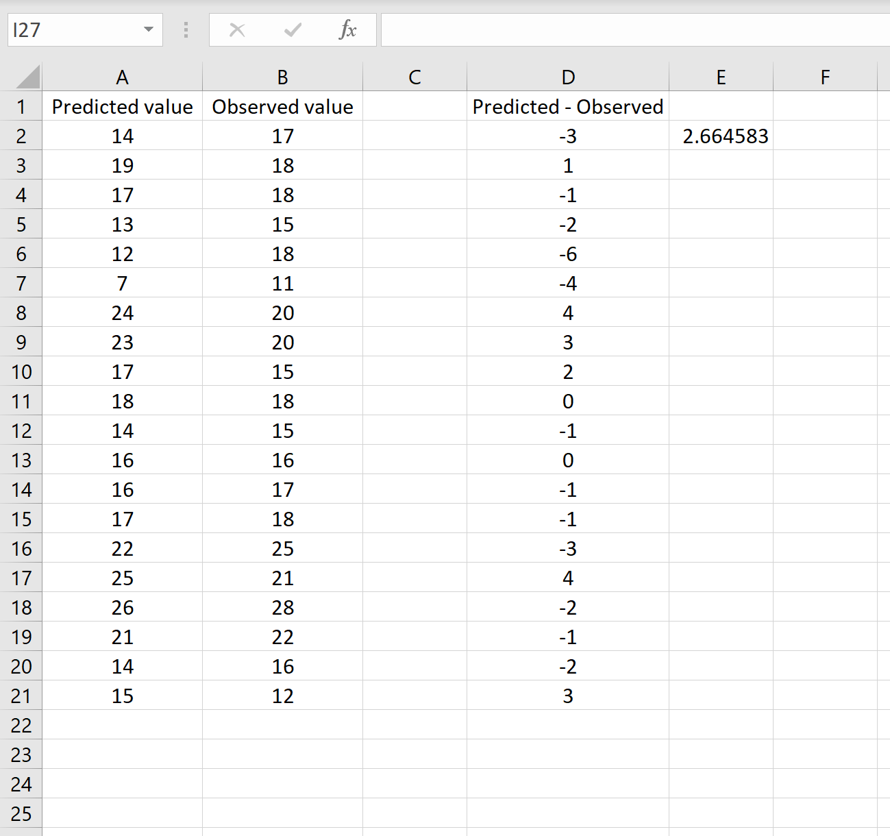
В одном сценарии у вас может быть один столбец, содержащий предсказанные значения вашей модели, и другой столбец, содержащий наблюдаемые значения. На изображении ниже показан пример такого сценария:

Если это так, то вы можете рассчитать RMSE, введя следующую формулу в любую ячейку, а затем нажав CTRL+SHIFT+ENTER:
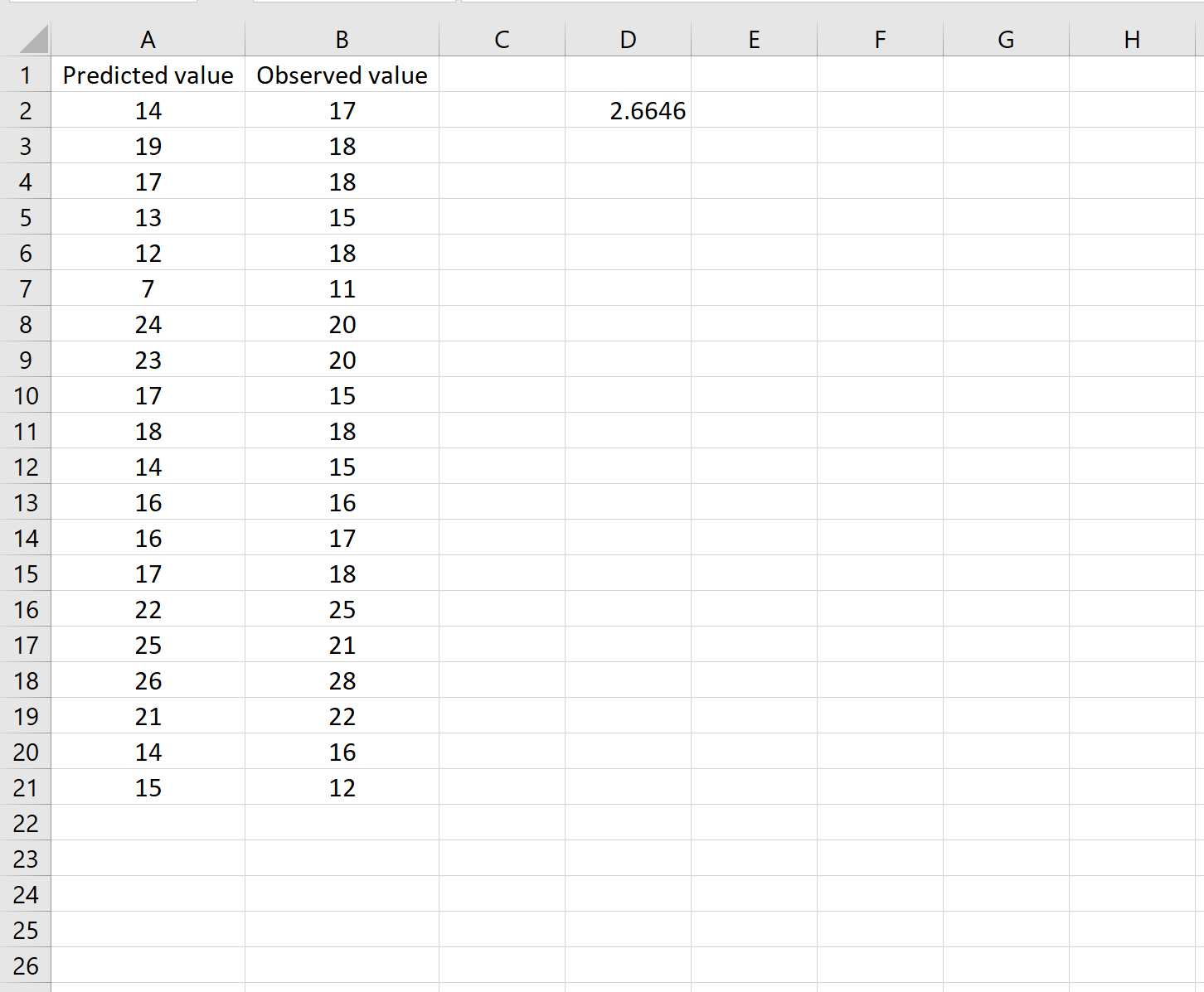
=КОРЕНЬ(СУММСК(A2:A21-B2:B21) / СЧЕТЧ(A2:A21))
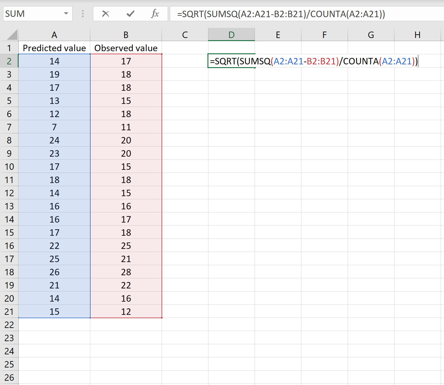
Это говорит нам о том, что среднеквадратическая ошибка равна 2,6646 .
Формула может показаться немного сложной, но она имеет смысл, если ее разобрать:
= КОРЕНЬ( СУММСК(A2:A21-B2:B21) / СЧЕТЧ(A2:A21) )
- Во-первых, мы вычисляем сумму квадратов разностей между прогнозируемыми и наблюдаемыми значениями, используя функцию СУММСК() .
- Затем мы делим на размер выборки набора данных, используя COUNTA() , который подсчитывает количество непустых ячеек в диапазоне.
- Наконец, мы извлекаем квадратный корень из всего вычисления, используя функцию SQRT() .
Сценарий 2
В другом сценарии вы, возможно, уже вычислили разницу между прогнозируемыми и наблюдаемыми значениями. В этом случае у вас будет только один столбец, отображающий различия.
На изображении ниже показан пример этого сценария. Прогнозируемые значения отображаются в столбце A, наблюдаемые значения — в столбце B, а разница между прогнозируемыми и наблюдаемыми значениями — в столбце D:
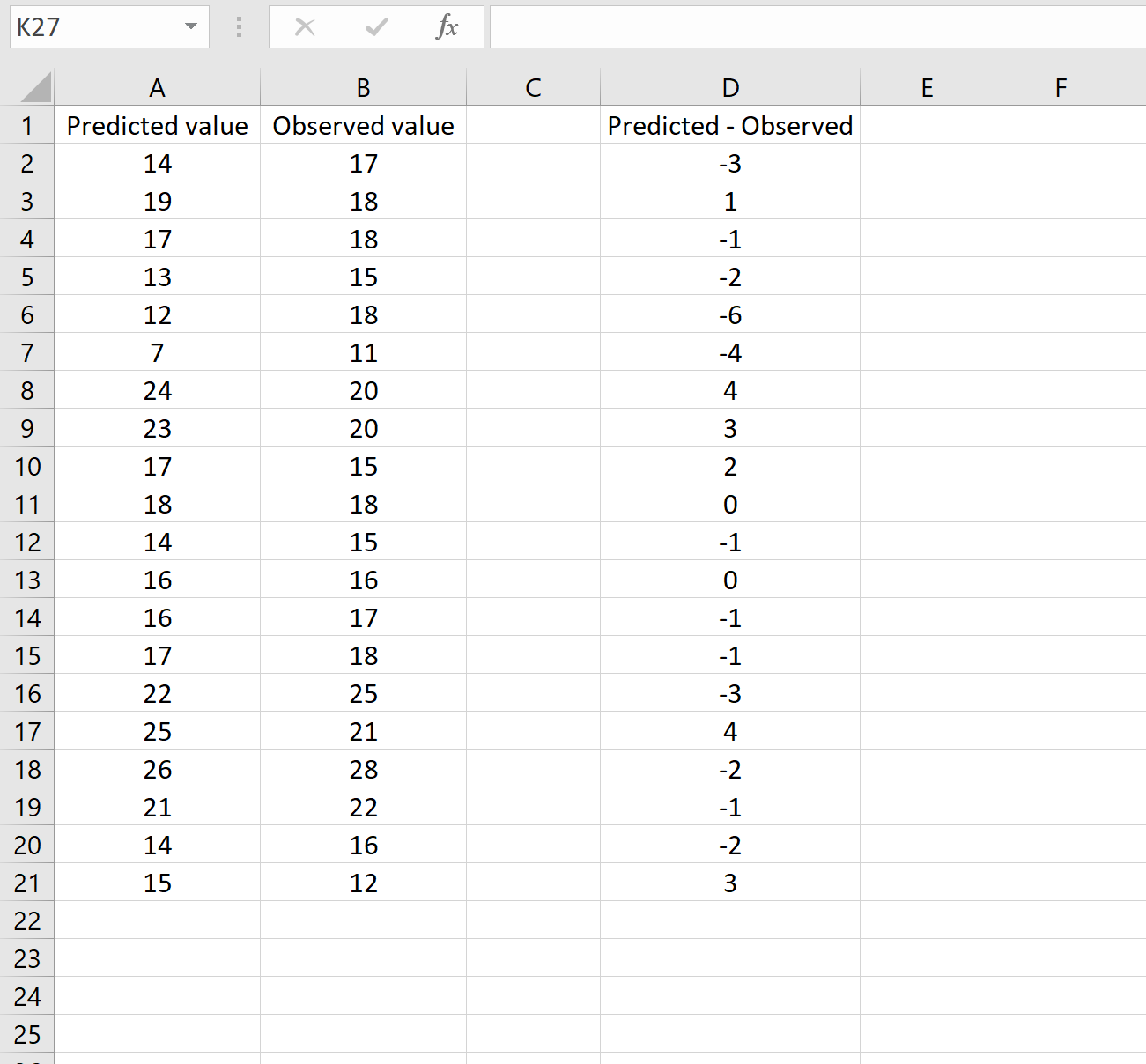
Если это так, то вы можете рассчитать RMSE, введя следующую формулу в любую ячейку, а затем нажав CTRL+SHIFT+ENTER:
=КОРЕНЬ(СУММСК(D2:D21) / СЧЕТЧ(D2:D21))
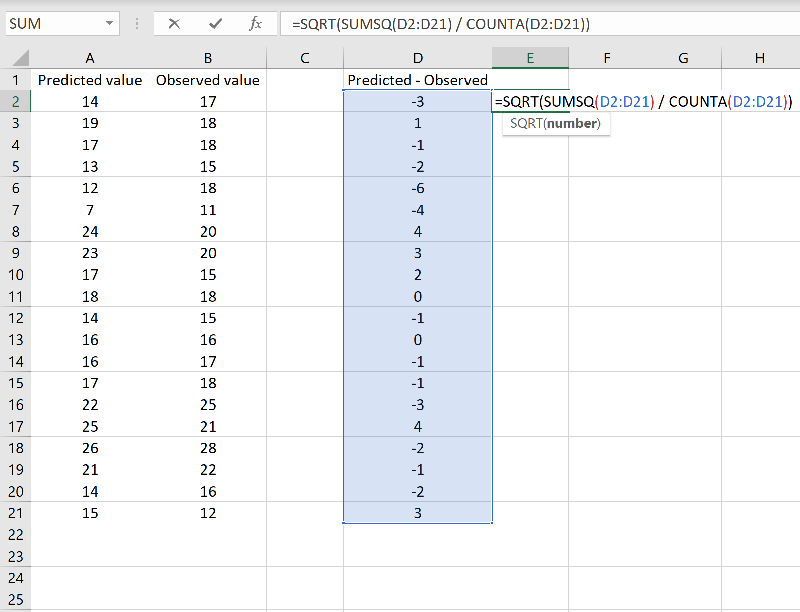
Это говорит нам о том, что среднеквадратическая ошибка равна 2,6646 , что соответствует результату, полученному в первом сценарии. Это подтверждает, что эти два подхода к расчету RMSE эквивалентны.
Формула, которую мы использовали в этом сценарии, лишь немного отличается от той, что мы использовали в предыдущем сценарии:
= КОРЕНЬ (СУММСК(D2 :D21) / СЧЕТЧ(D2:D21) )
- Поскольку мы уже рассчитали разницу между предсказанными и наблюдаемыми значениями в столбце D, мы можем вычислить сумму квадратов разностей с помощью функции СУММСК().только со значениями в столбце D.
- Затем мы делим на размер выборки набора данных, используя COUNTA() , который подсчитывает количество непустых ячеек в диапазоне.
- Наконец, мы извлекаем квадратный корень из всего вычисления, используя функцию SQRT() .
Как интерпретировать среднеквадратичную ошибку
Как упоминалось ранее, RMSE — это полезный способ увидеть, насколько хорошо регрессионная модель (или любая модель, которая выдает прогнозируемые значения) способна «соответствовать» набору данных.
Чем больше RMSE, тем больше разница между прогнозируемыми и наблюдаемыми значениями, а это означает, что модель регрессии хуже соответствует данным. И наоборот, чем меньше RMSE, тем лучше модель соответствует данным.
Может быть особенно полезно сравнить RMSE двух разных моделей друг с другом, чтобы увидеть, какая модель лучше соответствует данным.
Для получения дополнительных руководств по Excel обязательно ознакомьтесь с нашей страницей руководств по Excel , на которой перечислены все учебные пособия Excel по статистике.

Today we’re going to introduce some terms that are important to machine learning:
- Variance
- r2 score
- Mean square error
We illustrate these concepts using scikit-learn.
(This article is part of our scikit-learn Guide. Use the right-hand menu to navigate.)
Why these terms are important
You need to understand these metrics in order to determine whether regression models are accurate or misleading. Following a flawed model is a bad idea, so it is important that you can quantify how accurate your model is. Understanding that is not so simple.
These first metrics are just a few of them. Other concepts, like bias and overtraining models, also yield misleading results and incorrect predictions.
(Learn more in Bias and Variance in Machine Learning.)
To provide examples, let’s use the code from our last blog post, and add additional logic. We’ll also introduce some randomness in the dependent variable (y) so that there is some error in our predictions. (Recall that, in the last blog post we made the independent y and dependent variables x perfectly correlate to illustrate the basics of how to do linear regression with scikit-learn.)
What is variance?
In terms of linear regression, variance is a measure of how far observed values differ from the average of predicted values, i.e., their difference from the predicted value mean. The goal is to have a value that is low. What low means is quantified by the r2 score (explained below).
In the code below, this is np.var(err), where err is an array of the differences between observed and predicted values and np.var() is the numpy array variance function.
What is r2 score?
The r2 score varies between 0 and 100%. It is closely related to the MSE (see below), but not the same. Wikipedia defines r2 as
” …the proportion of the variance in the dependent variable that is predictable from the independent variable(s).”
Another definition is “(total variance explained by model) / total variance.” So if it is 100%, the two variables are perfectly correlated, i.e., with no variance at all. A low value would show a low level of correlation, meaning a regression model that is not valid, but not in all cases.
Reading the code below, we do this calculation in three steps to make it easier to understand. g is the sum of the differences between the observed values and the predicted ones. (ytest[i] – preds[i]) **2. y is each observed value y[i] minus the average of observed values np.mean(ytest). And then the results are printed thus:
print ("total sum of squares", y)
print ("ẗotal sum of residuals ", g)
print ("r2 calculated", 1 - (g / y))
Our goal here is to explain. We can of course let scikit-learn to this with the r2_score() method:
print("R2 score : %.2f" % r2_score(ytest,preds))
What is mean square error (MSE)?
Mean square error (MSE) is the average of the square of the errors. The larger the number the larger the error. Error in this case means the difference between the observed values y1, y2, y3, … and the predicted ones pred(y1), pred(y2), pred(y3), … We square each difference (pred(yn) – yn)) ** 2 so that negative and positive values do not cancel each other out.
The complete code
So here is the complete code:
import matplotlib.pyplot as plt
from sklearn import linear_model
import numpy as np
from sklearn.metrics import mean_squared_error, r2_score
reg = linear_model.LinearRegression()
ar = np.array([[[1],[2],[3]], [[2.01],[4.03],[6.04]]])
y = ar[1,:]
x = ar[0,:]
reg.fit(x,y)
print('Coefficients: n', reg.coef_)
xTest = np.array([[4],[5],[6]])
ytest =  np.array([[9],[8.5],[14]])
preds = reg.predict(xTest)
print("R2 score : %.2f" % r2_score(ytest,preds))
print("Mean squared error: %.2f" % mean_squared_error(ytest,preds))
er = []
g = 0
for i in range(len(ytest)):
print( "actual=", ytest[i], " observed=", preds[i])
x = (ytest[i] - preds[i]) **2
er.append(x)
g = g + x
x = 0
for i in range(len(er)):
x = x + er[i]
print ("MSE", x / len(er))
v = np.var(er)
print ("variance", v)
print ("average of errors ", np.mean(er))
m = np.mean(ytest)
print ("average of observed values", m)
y = 0
for i in range(len(ytest)):
y = y + ((ytest[i] - m) ** 2)
print ("total sum of squares", y)
print ("ẗotal sum of residuals ", g)
print ("r2 calculated", 1 - (g / y))
Results in:
Coefficients:
[[2.015]]
R2 score : 0.62
Mean squared error: 2.34
actual= [9.] observed= [8.05666667]
actual= [8.5] observed= [10.07166667]
actual= [14.] observed= [12.08666667]
MSE [2.34028611]
variance 1.2881398892129619
average of errors 2.3402861111111117
average of observed values 10.5
total sum of squares [18.5]
ẗotal sum of residuals [7.02085833]
r2 calculated [0.62049414]
You can see by looking at the data np.array([[[1],[2],[3]], [[2.01],[4.03],[6.04]]]) that every dependent variable is roughly twice the independent variable. That is confirmed as the calculated coefficient reg.coef_ is 2.015.
There is no correct value for MSE. Simply put, the lower the value the better and 0 means the model is perfect. Since there is no correct answer, the MSE’s basic value is in selecting one prediction model over another.
Similarly, there is also no correct answer as to what R2 should be. 100% means perfect correlation. Yet, there are models with a low R2 that are still good models.
Our take away message here is that you cannot look at these metrics in isolation in sizing up your model. You have to look at other metrics as well, plus understand the underlying math. We will get into all of this in subsequent blog posts.
Additional Resources
Extending R-squared beyond ordinary least-squares linear regression from pcdjohnson
Learn ML with our free downloadable guide
This e-book teaches machine learning in the simplest way possible. This book is for managers, programmers, directors – and anyone else who wants to learn machine learning. We start with very basic stats and algebra and build upon that.

These postings are my own and do not necessarily represent BMC’s position, strategies, or opinion.
See an error or have a suggestion? Please let us know by emailing blogs@bmc.com.
BMC Brings the A-Game
BMC works with 86% of the Forbes Global 50 and customers and partners around the world to create their future. With our history of innovation, industry-leading automation, operations, and service management solutions, combined with unmatched flexibility, we help organizations free up time and space to become an Autonomous Digital Enterprise that conquers the opportunities ahead.
Learn more about BMC ›
You may also like
About the author

Walker Rowe
Walker Rowe is an American freelancer tech writer and programmer living in Cyprus. He writes tutorials on analytics and big data and specializes in documenting SDKs and APIs. He is the founder of the Hypatia Academy Cyprus, an online school to teach secondary school children programming. You can find Walker here and here.
What is mean squared error (MSE)?
The mean squared error, or MSE, is a performance metric that indicates how well your model fits the target. The mean squared error is defined as the average of all squared differences between the true and predicted values:
$$mathrm{MSE}=frac{1}{n}sum^{n-1}_{i=0}(y_i-hat{y}_i)^2$$
Where:
-
$n$ is the number of predicted values
-
$y_i$ is the actual true value of the $i$-th data
-
$hat{y}_i$ is the predicted value of the $i$-th data
A high value of MSE means that the model is not performing well, whereas a MSE of 0 would mean that you have a perfect model that predicts the target without any error.
Simple example of computing mean squared error (MSE)
Suppose we are given the three data points (1,3), (2,2) and (3,2). To predict the y-value given the x-value, we’ve built a simple learn curve, $y=x$, as shown below:
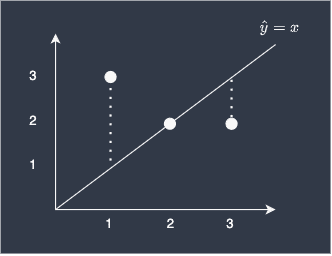
We can see that we are off by 2 for the first data point, the prediction is perfect for the second point, and off by 1 for the last point.
To quantify how good our model is, we can compute the MSE like so:
$$begin{align*}
mathrm{MSE}&=frac{1}{3}left[(1-3)^2+(2-2)^2+(3-2)^2right]\
&=frac{1}{3}left(4+0+1right)\
&approx1.67
end{align*}$$
This means that the average squared differences between the true value and the predicted value is 1.67.
Intuition behind mean squared error (MSE)
Interpretation of MSE
MSE is defined as the average squared differences between the actual values and the predicted values. This makes the interpretation of MSE rather awkward since the unit of MSE is not the same as the unit of the y-values due to squaring the differences. Therefore, we typically interpret a high value of MSE as indicative of a poor-performing model, while a low value of MSE as indicative of a decent model.
There is another performance metric called root mean squared error (RMSE), which is simply the square root of MSE. This means that the RMSE takes on the same unit as that of the target values, which implies you can loosely interpret RMSE as the average difference between the actual and predicted values.
Why are we squaring the difference?
The reason we take the square when calculating MSE is that we care only about the magnitude of the differences between true and predicted value — we do not want the positive and negative differences cancelling each other out. For example, consider the following case:
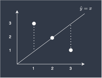
Suppose we computed the MSE without taking the square:
$$frac{1}{3}left[(1-3)+(2-2)+(3-1)right]=0$$
You can see that the negative difference and the positive difference of the first and third data points cancel each other out, resulting in a misleading error benchmark of 0. Of course, we know that the model is far from perfect in reality. In order to avoid such problems, we square the differences.
Why don’t we just take the absolute difference instead?
You may be wondering why we don’t just take the absolute difference between the true and predicted value if all we care about is the magnitude of the differences. In fact, there is another popular metric called mean absolute error (MAE) that does just this. The advantage of absolute mean error is that the interpretation is simple — the error is just how off your predictions are from the true value on average.
The caveat, however, is that it is not easy to find minimum values of MAE, which means that it is challenging to train a model that minimises MAE. On the other hand, MSE is easily differentiable and hence easy to optimise. This is reason why MSE is preferred over MAE as the cost function of machine learning models.
Computing the mean squared error (MSE) in Python’s Scikit-learn
Let’s compute the MSE for the example above using Python’s scikit-learn library. To compute the MSE in scikit-learn, simply use the mean_squared_error method:
from sklearn.metrics import mean_squared_error
y_true = [1,2,3]
y_pred = [3,2,2]
mean_squared_error(y_true, y_pred)
1.6666666666666667
We can see that the outputted MSE is exactly the same as the value we manually calculated above.
Setting multioutput
By default, multioutput='uniform_average', which returns a the global mean squared error:
y_true = [[1,2],[3,4]]
y_pred = [[6,7],[9,8]]
mean_squared_error(y_true, y_pred)
25.5
Setting multioutput='raw_values' will return mean squared error of each column:
y_true = [[1,2],[3,4]]
y_pred = [[6,7],[9,8]]
mean_squared_error(y_true, y_pred, multioutput='raw_values')
array([30.5, 20.5])
Here, 30.5 is calculated as:
((1-6)^2 + (3-9)^2) / 2 = 30.5
В большинстве описаний среднеквадратичной ошибки (mean square errore, MSE) упускается один важнейший нюанс: метрики и функции потерь — это не совсем одно и то же. Для оценки и оптимизации производительности модели в машинном обучении нужны две отдельные функции потерь. MSE может быть либо тем, либо другим, либо третьим — выбор за исследователем.
Чтобы было понятнее, что имеется в виду под оценкой производительности и оптимизацией, вместо отвлеченных рассуждений обратимся к конкретным примерам. Для демонстрации будем использовать среднеквадратичную ошибку (MSE), но имейте в виду: MSE — это полезная метрика, но не панацея. Итак, погрузимся в тему!
https://t.me/python_job_interview
Что такое MSE?
Среднеквадратичная ошибка (MSE) — одна из множества метрик, которые используются для оценки эффективности модели. Для расчета MSE необходимо возвести в квадрат количество обнаруженных ошибок и найти среднее значение.
Зачем вычислять MSE?
Это можно сделать для 2 целей.
- Оценка производительности — визуальное определение того, насколько хорошо работает модель. Другими словами, это возможность быстро понять, с чем предстоит работать.
- Оптимизация модели позволяет выяснить, достигнуто ли наилучшее из возможных соответствий или же требуются улучшения. Другими словами, определить, какая модель максимально подходит для работы с выбранными точками данных.
Если вы предпочитаете учиться на видео, переходите по этой ссылке (англ. язык):
https://youtube.com/watch?v=j8VjRnaHRBM%3Ffeature%3Doembed
Оценка производительности (метрика)
Цель оценки производительности заключается в том, чтобы человек мог составить представление об эффективности модели.
Метрика производительности показывает, насколько хорошо работает модель. К слову, “модель” — это просто популярное слово для “инструкции”, а инструкция “хороша”, если при введении исходных данных обеспечивает результат, близкий к ожидаемому. Метрика позволяет оценить, насколько близки результаты модели к ожидаемым (причем исследователь сам должен определить, что значит “близки”). MSE — это всего лишь одна из многих возможных метрик.
ЕСЛИ МОДЕЛЬ СОВЕРШЕННА, MSE = 0.
Откуда берется MSE? Мы вычисляем эту метрику, находя ошибки, которые допустила модель. Поэтому она является функцией ошибочности. Чем ниже MSE, тем лучше работает модель. Когда ошибок совсем нет, MSE = 0. Беглый взгляд на MSE дает представление о том, насколько хорошо модель соответствует или не соответствует данным.

Взглянув на MSE двух моделей из примера со смузи в моем курсе (смотрите видео здесь), можно легко определить фаворита. Модель с меньшим MSE (2381, а не 7157) лучше подходит к данным. Но что означают эти цифры?
МЕТРИКИ ДОЛЖНЫ БЫТЬ РАССЧИТАНЫ ТАК, ЧТОБЫ ИМЕТЬ СМЫСЛ ДЛЯ ЛЮДЕЙ И ЭФФЕКТИВНО ПЕРЕДАВАТЬ ИНФОРМАЦИЮ.
Приведенные выше значения MSE не очень удобны для осмысления. Это проблема, если нужна достаточно информативная метрика. Метрики должны быть рассчитаны так, чтобы иметь смысл для людей и эффективно передавать информацию. Можно ли улучшить значение MSE?
Да, конечно. Вот вам RMSE!
Для оценки производительности модели (на глаз) RMSE часто является лучшим выбором, чем MSE. RMSE — это просто корень квадратный из MSE (R означает root, “корень”).

При поиске более подходящей метрики, исследователи предпочитают RMSE, потому что она переводит MSE в более понятную для человека шкалу. Это не совсем то, что покажет, “насколько велики наши ошибки в среднем”, но достаточно близко к тому, что можно принять во внимание, чтобы предотвратить риски.
ИССЛЕДОВАТЕЛИ ПРЕДПОЧИТАЮТ RMSE, ПОТОМУ ЧТО ЭТА МЕТРИКА ПЕРЕВОДИТ MSE В БОЛЕЕ УДОБНУЮ ДЛЯ ВОСПРИЯТИЯ ШКАЛУ.
Но что если вы настаиваете на еще более точной метрике — той, что даст корректное представление о среднем размере ошибок? В таком случае можно воспользоваться метрикой, называемой средним абсолютным отклонением или MAD (mean absolute deviation). Иногда ее также называют MAE (mean absolute error).
Чтобы вычислить MAD, нужно просто игнорировать знаки (“+” и “-”) перед значениями всех ошибок и найти среднее значение. В отличие от RMSE, MAD является абсолютным выражением среднего размера ошибок.
MAD ПОКАЗЫВАЕТ, НАСКОЛЬКО ОШИБОЧНА МОДЕЛЬ В СРЕДНЕМ.
MAD — лучшая метрика производительности по сравнению с RMSE, потому что ее легче понять и связать с процессом оптимизации. Она более значима для исследователя и понятнее для человека. Но подходит ли она для машин?
Оптимизация модели (функция потерь)
Вторая цель использования MSE — это оптимизация модели. Здесь в дело вступают функции потерь.
Функция потерь — это формула, которую алгоритм машинного обучения пытается минимизировать на этапе оптимизации/подгонки модели. Разложим это понятие по полочкам.
https://youtube.com/watch?v=I2Ek0icqMXE%3Ffeature%3Doembed
Фрагмент из курса MFML для тех, кому нужно освежить в памяти понятие оптимизации модели
Предположим, планируется использование одного из самых простых алгоритмов МО — OLS (ordinary least squares, метод простых наименьших квадратов). Это означает, что модель, с которой предстоит работать, обладает простейшей формой — прямой линией.
Линия, проведенная через данные, имеет наклон и точку пересечения с координатной осью. Установка этих двух параметров зависит от вас!
Y = ТОЧКА ПЕРЕСЕЧЕНИЯ + НАКЛОН * X
Рациональный подход требует выбора модели, которая лучше всего подходит для работы с исходными данными. Другими словами, оптимальным выбором будет модель, которая максимально адаптирована к исходным данным. Следовательно, нужна функция оценки, которая становится больше, когда модель подходит хуже, и меньше — в обратном случае.
Эта функция позволит изменять параметры точки пересечения и наклона, наблюдая за изменением оценки. Такую функцию оценки называют “функцией потерь” — чем больше потери, тем хуже модель.
Ошибочность? Заядлые перфекционисты уверены: ошибки — это плохо. Поэтому выразим ошибочность в терминах наших ошибок. Любая функция потерь, которая становится больше, когда больше ошибок, подойдет? Технически — да. Практически — нет.
Вот как это работает, если выбрать MSE в качестве функции потерь: цель оптимизации — найти точку пересечения и наклон, которые дают как можно более низкое значение MSE. Как это происходит, показано в видео ниже.
https://youtube.com/watch?v=j8VjRnaHRBM%3Ffeature%3Doembed
Не стоит искать оптимальное значение MSE методом проб и ошибок (перебирание различных комбинаций наклона и точки пересечения вручную — медленный и скучный процесс).
Получить мгновенный результат позволят вычисления или алгоритм оптимизации, которые подскажут, какими должны быть необходимые параметры. Что касается алгоритмов оптимизации, то вам, скорей всего, не придется разрабатывать их с нуля. Наверняка будет возможность импортировать те, которые кто-то другой уже создал. Чаще всего с MSE очень удобно работать.

Что же происходит “за кулисами”? Есть формула, которая указывает, где именно должна располагаться линия, чтобы значение MSE было минимальным. Запускаемому коду даже не нужно постепенно приближаться к решению — он просто использует эту формулу, чтобы точно указать наклон и точку пересечения, наилучшие из возможных для работы линейной модели с данными.
источник
Просмотры: 821
Created by Anna Szczepanek, PhD
Reviewed by
Wojciech Sas, PhD and Jack Bowater
Last updated:
Nov 12, 2022
Omni’s MSE calculator is here for you whenever you need to quickly determine the sum of squared errors (SSE) and mean squared error (MSE) when searching for the line of best fit. You can also use this tool if you are wondering how to calculate MSE by hand, since it can show you the results of intermediate calculations.
Not sure what MSE is? Need just the formula for MSE, or rather looking for a precise mathematical definition of MSE and an explanation of the reasoning behind it? You’re in the right place! Scroll down to learn everything you need about MSE in statistics! An example of MSE calculated step-by-step is also included for your convenience!
What is MSE in statistics?
In statistics, the mean squared error (MSE) measures how close predicted values are to observed values. Mathematically, MSE is the average of the squared differences between the predicted values and the observed values. We often use the term residuals to refer to these individual differences.
We most often define the predicted values as the values obtained from simple linear regression, or just as the arithmetic mean of the observed values — in the latter case, all the predicted values are equal.
💡 In simple linear regression, the line of best fit found via the method of least squares is exactly the line that minimizes MSE! See the linear regression calculator to learn the details.
We now have a basic idea of what MSE is, so it’s time to quickly explain how to find MSE with the help of our mean square error calculator.
How to use this MSE calculator?
It can’t be any simpler! To use our MSE calculator most efficiently, follow these steps:
-
Choose the mode of the mean square error calculator — should the predicted values be automatically set as the average of the observed values, or do you want to enter custom values?
-
Next, input your data. You can enter up to 30 values — the fields will appear as you go.
-
The MSE and SSE of your observations are already there!
-
Do you want to see some of the details of the calculations? Turn the
Show details?option toYes!Tip: This option allows you to use this calculator to generate examples of MSE!
-
You can also increase the precision of calculations — just click the
advanced modeand adjust thePrecisionvalue.
As nice as it is to use Omni’s MSE calculator, it may happen that you’ll have to compute MSE or SSE by hand. In the next section, we’ll provide you with all the formulas you need.
How to find MSE and SSE?
Let x1, …, xn be the observed values and y1, …, yn be the predicted values.
The equation for MSE is the following:
MSE = (1/n) * Σi(xi— yi)²,
where i runs from 1 to n.
If we ignore the 1/n factor in front of the sum, we arrive at the formula for SSE:
SSE = Σi(xi— yi)²,
where i runs from 1 to n. In other words, the relationship between SSE and MSE is the following:
MSE = SSE / n.
Matrix formula for MSE
Let us consider the column-vector e with coefficients defined as
ei = xi — yi
for i = 1, ..., n. That is, e is the vector of residuals.
Using e, we can say that MSE is equal to 1/n times the squared magnitude of e, or 1/n times the dot product of e by itself:
MSE = (1/n) * |e|² = (1/n) * e ∙ e.
Alternatively, we can rewrite this MSE equation as follows:
MSE = (1/n) * eTe,
where eT is the transpose of e, i.e., a row-vector.
The above formulas lead us immediately to the following expression for SSE:
SSE = |e|² = e ∙ e = eTe.
If you’re not yet familiar with the notions we’ve used above, discover them with our dedicated tool:
- Dot product calculator; and
- Matrix transpose calculator.
Why do we take squares in MSE?
Wouldn’t it be simpler and more intuitive to add the differences between actual data and predictions without squaring them first?
No, there are good reasons for taking the squares!
Namely, the predicted values can be greater than or less than the observed values. And when we add together positive and negative differences, individual errors may cancel each other out. As a result, we can get the sum close to (or even equal to) zero even though the terms were relatively large. This could lead us to a false conclusion that our prediction is accurate since the error is low.
In contrast, when we take a square of each difference, we get a positive number, and each individual error increases the sum. In other words, squaring makes both positive and negative differences contribute to the final value in the same way. Thanks to squaring, we can say that the smaller the value of MSE, the better model.
In particular, if the predicted values coincided perfectly with observed values, then MSE would be zero. This, however, nearly never happens in practice: MSE is almost always strictly positive because there’s almost always some noise (randomness) in the observed values.
As you can see, we really can’t take simple differences. However, squares are not the only option! In the next section, we will tell you, among other things, about MAE, which uses absolute values instead of squares to achieve exactly the same effect — get rid of negative signs of differences.
Alternatives to MSE in statistics
As we’ve seen in the formulas, the units of MSE are the square of the original units, exactly like in the case of variance. To return to the original units, we often take the square root of MSE, obtaining the root mean squared error (RMSE):
RMSE = √MSE,
This is analogous to taking the square root of variance in order to get the standard deviation.
Another (slightly less popular) measure of the quality of prediction is the mean absolute error (MAE), where, instead of squaring the differences between observed and predicted values, we take the absolute differences between them:
MAE = (1/n) * Σi|xi— yi|,
where i runs from 1 to n. When the predicted values are all equal to the mean of observed values, we arrive at the mean absolute deviation.
MSE example
Phew, we’re finally done with the definition of MSE and all the formulas. It’s high time we looked at an example!
Assume we have the following data:
3, 15, 6, 3, 44, 8, 15, 9, 7, 25, 24, 5, 88, 44, 3, 21.
-
We see there are sixteen numbers, so
n = 16. -
Next, we compute the average:
(3 + 15 + 6 + 3 + 44 + 8 + 15 + 9 + 7 + 25 + 24 + 5 + 88 + 44 + 3 + 21) / 16 = 320 / 16 = 20.Hence,
μ = 20. -
We compute the differences between each observation and the mean
μand also their squares:
|
x |
x — μ |
(x — μ)² |
|---|---|---|
|
3 |
-17 |
289 |
|
15 |
-5 |
25 |
|
6 |
-14 |
196 |
|
3 |
-17 |
289 |
|
44 |
24 |
576 |
|
8 |
-12 |
144 |
|
15 |
-5 |
25 |
|
9 |
-11 |
121 |
|
7 |
-13 |
169 |
|
25 |
5 |
25 |
|
24 |
4 |
16 |
|
5 |
-15 |
225 |
|
88 |
68 |
4624 |
|
44 |
24 |
576 |
|
3 |
-17 |
289 |
|
21 |
1 |
1 |
-
We sum the numbers from the 3rd column:
289 + 25 + 196 + 189 + 576 + 144 + 25 + 121 + 169 + 25 + 16 + 225 + 4624 + 576 + 289 + 1 = 7590,
to get their SSE:SSE = 7590. -
To find MSE, we divide SSE by the sample length
n = 16:MSE = 7590 / 16 = 474.40. -
To find RMSE, we take the square root of MSE:
RMSE = √474.40 ≈ 21.78.
FAQ
How do I calculate MSE by hand?
To calculate MSE by hand, follow these instructions:
- Compute differences between the observed values and the predictions.
- Square each of these differences.
- Add all these squared differences together.
- Divide this sum by the sample length.
- That’s it, you’ve found the MSE of your data!
How do I calculate SSE from MSE?
If you’re given MSE, just one simple step separates you from finding SSE! The only thing you need to know is the sample length n. Then apply this formula:
SSE = MSE × n
and enjoy your newly-computed SSE!
How do I calculate RMSE from MSE?
To calculate RMSE from MSE, you need to remember that RMSE is the abbreviation of the root mean sum of errors, so, as its name indicates, RMSE is just the square root of MSE:
RMSE = √MSE.
How do I calculate RMSE from SSE?
In order to correctly calculate RMSE from SSE, recall that RMSE is the square root of MSE, which, in turn, is SSE divided by the sample length n. Combining these two formulas, we arrive at the following direct relationship between RMSE and SSE:
RMSE = √(SSE / n).
Calculator mode
What are the predicted values?
Data (You may enter up to 30 points)
5 number summary5★ rating averageCoefficient of variation… 36 more