Last Updated on July 1, 2021
Would you have guessed that I’m a stamp collector?
Just kidding. I’m not.
But let’s play a little game of pretend.
Let’s pretend that we have a huge dataset of stamp images. And we want to take two arbitrary stamp images and compare them to determine if they are identical, or near identical in some way.
In general, we can accomplish this in two ways.
The first method is to use locality sensitive hashing, which I’ll cover in a later blog post.
The second method is to use algorithms such as Mean Squared Error (MSE) or the Structural Similarity Index (SSIM).
In this blog post I’ll show you how to use Python to compare two images using Mean Squared Error and Structural Similarity Index.
- Update July 2021: Updated SSIM import from scikit-image per the latest API update. Added section on alternative image comparison methods, including resources on siamese networks.
![]()
Looking for the source code to this post?
Jump Right To The Downloads Section
Our Example Dataset
Let’s start off by taking a look at our example dataset:
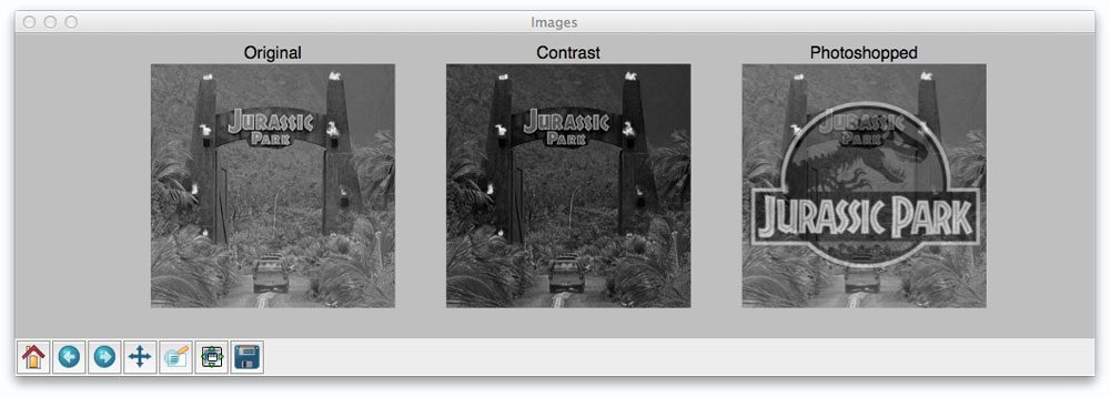
Here you can see that we have three images: (left) our original image of our friends from Jurassic Park going on their first (and only) tour, (middle) the original image with contrast adjustments applied to it, and (right), the original image with the Jurassic Park logo overlaid on top of it via Photoshop manipulation.
Now, it’s clear to us that the left and the middle images are more “similar” to each other — the one in the middle is just like the first one, only it is “darker”.
But as we’ll find out, Mean Squared Error will actually say the Photoshopped image is more similar to the original than the middle image with contrast adjustments. Pretty weird, right?
Mean Squared Error vs. Structural Similarity Measure
Let’s take a look at the Mean Squared error equation:
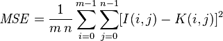
While this equation may look complex, I promise you it’s not.
And to demonstrate this you, I’m going to convert this equation to a Python function:
def mse(imageA, imageB):
	# the 'Mean Squared Error' between the two images is the
	# sum of the squared difference between the two images;
	# NOTE: the two images must have the same dimension
	err = np.sum((imageA.astype("float") - imageB.astype("float")) ** 2)
	err /= float(imageA.shape[0] * imageA.shape[1])

	# return the MSE, the lower the error, the more "similar"
	# the two images are
	return err
So there you have it — Mean Squared Error in only four lines of Python code once you take out the comments.
Let’s tear it apart and see what’s going on:
- On Line 7 we define our
msefunction, which takes two arguments:imageAandimageB(i.e. the images we want to compare for similarity). - All the real work is handled on Line 11. First we convert the images from unsigned 8-bit integers to floating point, that way we don’t run into any problems with modulus operations “wrapping around”. We then take the difference between the images by subtracting the pixel intensities. Next up, we square these difference (hence mean squared error, and finally sum them up.
- Line 12 handles the mean of the Mean Squared Error. All we are doing is dividing our sum of squares by the total number of pixels in the image.
- Finally, we return our MSE to the caller one Line 16.
MSE is dead simple to implement — but when using it for similarity, we can run into problems. The main one being that large distances between pixel intensities do not necessarily mean the contents of the images are dramatically different. I’ll provide some proof for that statement later in this post, but in the meantime, take my word for it.
It’s important to note that a value of 0 for MSE indicates perfect similarity. A value greater than one implies less similarity and will continue to grow as the average difference between pixel intensities increases as well.
In order to remedy some of the issues associated with MSE for image comparison, we have the Structural Similarity Index, developed by Wang et al.:
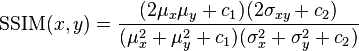
The SSIM method is clearly more involved than the MSE method, but the gist is that SSIM attempts to model the perceived change in the structural information of the image, whereas MSE is actually estimating the perceived errors. There is a subtle difference between the two, but the results are dramatic.
Furthermore, the equation in Equation 2 is used to compare two windows (i.e. small sub-samples) rather than the entire image as in MSE. Doing this leads to a more robust approach that is able to account for changes in the structure of the image, rather than just the perceived change.
The parameters to Equation 2 include the (x, y) location of the N x N window in each image, the mean of the pixel intensities in the x and y direction, the variance of intensities in the x and y direction, along with the covariance.
Unlike MSE, the SSIM value can vary between -1 and 1, where 1 indicates perfect similarity.
Luckily, as you’ll see, we don’t have to implement this method by hand since scikit-image already has an implementation ready for us.
Let’s go ahead and jump into some code.
# import the necessary packages
from skimage.metrics import structural_similarity as ssim
import matplotlib.pyplot as plt
import numpy as np
import cv2
We start by importing the packages we’ll need — matplotlib for plotting, NumPy for numerical processing, and cv2 for our OpenCV bindings. Our Structural Similarity Index method is already implemented for us by scikit-image, so we’ll just use their implementation.
def mse(imageA, imageB):
	# the 'Mean Squared Error' between the two images is the
	# sum of the squared difference between the two images;
	# NOTE: the two images must have the same dimension
	err = np.sum((imageA.astype("float") - imageB.astype("float")) ** 2)
	err /= float(imageA.shape[0] * imageA.shape[1])

	# return the MSE, the lower the error, the more "similar"
	# the two images are
	return err

def compare_images(imageA, imageB, title):
	# compute the mean squared error and structural similarity
	# index for the images
	m = mse(imageA, imageB)
	s = ssim(imageA, imageB)

	# setup the figure
	fig = plt.figure(title)
	plt.suptitle("MSE: %.2f, SSIM: %.2f" % (m, s))

	# show first image
	ax = fig.add_subplot(1, 2, 1)
	plt.imshow(imageA, cmap = plt.cm.gray)
	plt.axis("off")

	# show the second image
	ax = fig.add_subplot(1, 2, 2)
	plt.imshow(imageB, cmap = plt.cm.gray)
	plt.axis("off")

	# show the images
	plt.show()
Lines 7-16 define our mse method, which you are already familiar with.
We then define the compare_images function on Line 18 which we’ll use to compare two images using both MSE and SSIM. The mse function takes three arguments: imageA and imageB, which are the two images we are going to compare, and then the title of our figure.
We then compute the MSE and SSIM between the two images on Lines 21 and 22.
Lines 25-39 handle some simple matplotlib plotting. We simply display the MSE and SSIM associated with the two images we are comparing.
# load the images -- the original, the original + contrast,
# and the original + photoshop
original = cv2.imread("images/jp_gates_original.png")
contrast = cv2.imread("images/jp_gates_contrast.png")
shopped = cv2.imread("images/jp_gates_photoshopped.png")

# convert the images to grayscale
original = cv2.cvtColor(original, cv2.COLOR_BGR2GRAY)
contrast = cv2.cvtColor(contrast, cv2.COLOR_BGR2GRAY)
shopped = cv2.cvtColor(shopped, cv2.COLOR_BGR2GRAY)
Lines 43-45 handle loading our images off disk using OpenCV. We’ll be using our original image (Line 43), our contrast adjusted image (Line 44), and our Photoshopped image with the Jurassic Park logo overlaid (Line 45).
We then convert our images to grayscale on Lines 48-50.
# initialize the figure
fig = plt.figure("Images")
images = ("Original", original), ("Contrast", contrast), ("Photoshopped", shopped)

# loop over the images
for (i, (name, image)) in enumerate(images):
	# show the image
	ax = fig.add_subplot(1, 3, i + 1)
	ax.set_title(name)
	plt.imshow(image, cmap = plt.cm.gray)
	plt.axis("off")

# show the figure
plt.show()

# compare the images
compare_images(original, original, "Original vs. Original")
compare_images(original, contrast, "Original vs. Contrast")
compare_images(original, shopped, "Original vs. Photoshopped")
Now that our images are loaded off disk, let’s show them. On Lines 52-65 we simply generate a matplotlib figure, loop over our images one-by-one, and add them to our plot. Our plot is then displayed to us on Line 65.
Finally, we can compare our images together using the compare_images function on Lines 68-70.
We can execute our script by issuing the following command:
$ python compare.py
Results
Once our script has executed, we should first see our test case — comparing the original image to itself:
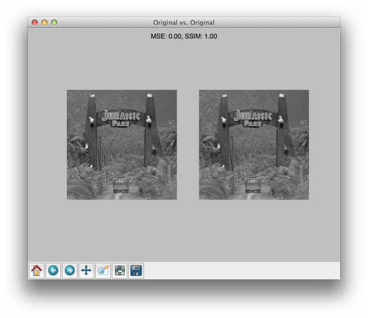
Not surpassingly, the original image is identical to itself, with a value of 0.0 for MSE and 1.0 for SSIM. Remember, as the MSE increases the images are less similar, as opposed to the SSIM where smaller values indicate less similarity.
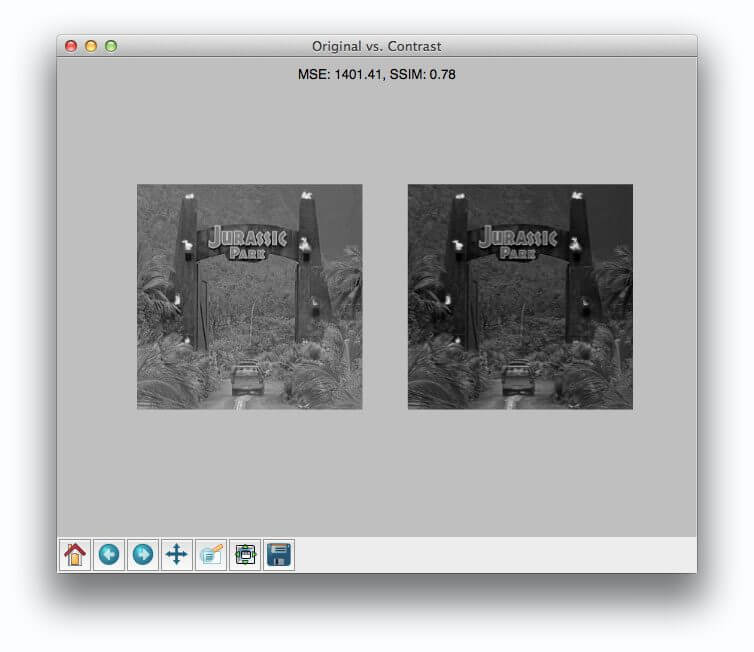
Now, take a look at comparing the original to the contrast adjusted image:
In this case, the MSE has increased and the SSIM decreased, implying that the images are less similar. This is indeed true — adjusting the contrast has definitely “damaged” the representation of the image.
But things don’t get interesting until we compare the original image to the Photoshopped overlay:
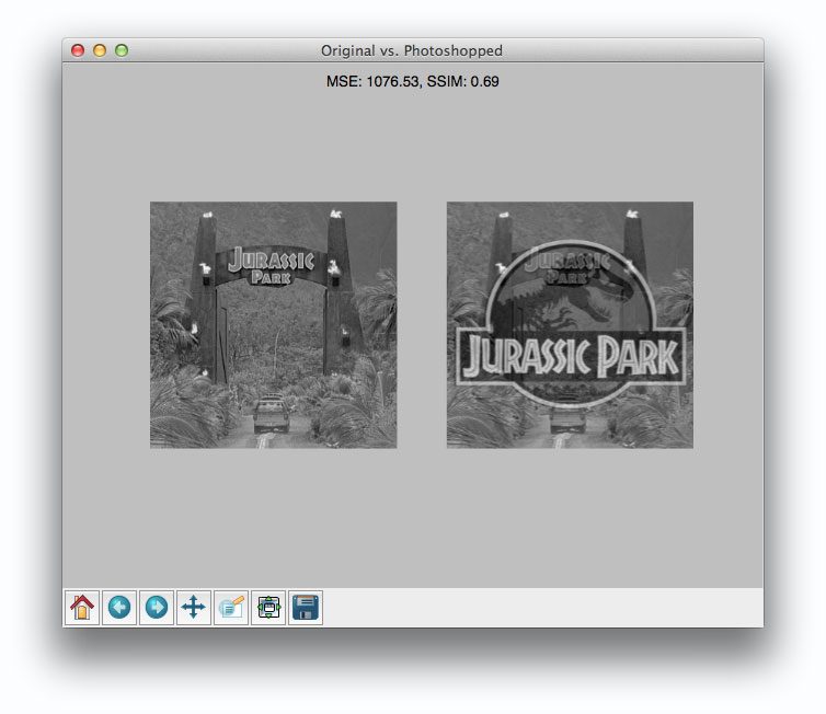
Comparing the original image to the Photoshop overlay yields a MSE of 1076 and a SSIM of 0.69.
Wait a second.
A MSE of 1076 is smaller than the previous of 1401. But clearly the Photoshopped overlay is dramatically more different than simply adjusting the contrast! But again, this is a limitation we must accept when utilizing raw pixel intensities globally.
On the other end, SSIM is returns a value of 0.69, which is indeed less than the 0.78 obtained when comparing the original image to the contrast adjusted image.
Alternative Image Comparison Methods
MSE and SSIM are traditional computer vision and image processing methods to compare images. They tend to work best when images are near-perfectly aligned (otherwise, the pixel locations and values would not match up, throwing off the similarity score).
An alternative approach that works well when the two images are captured under different viewing angles, lighting conditions, etc., is to use keypoint detectors and local invariant descriptors, including SIFT, SURF, ORB, etc. This tutorial shows you how to implement RootSIFT, a more accurate variant of the popular SIFT detector and descriptor.
Furthermore, there are deep learning-based image similarity methods that we can utilize, particularly siamese networks. Siamese networks are super powerful models that can be trained with very little data to compute accurate image similarity scores.
The following tutorials will teach you about siamese networks:
- Building image pairs for siamese networks with Python
- Siamese networks with Keras, TensorFlow, and Deep Learning
- Comparing images for similarity using siamese networks, Keras, and TensorFlow
Additionally, siamese networks are covered in detail inside PyImageSearch University.
What’s next? I recommend PyImageSearch University.
Course information:
69 total classes • 73 hours of on-demand code walkthrough videos • Last updated: February 2023
★★★★★ 4.84 (128 Ratings) • 15,800+ Students Enrolled
I strongly believe that if you had the right teacher you could master computer vision and deep learning.
Do you think learning computer vision and deep learning has to be time-consuming, overwhelming, and complicated? Or has to involve complex mathematics and equations? Or requires a degree in computer science?
That’s not the case.
All you need to master computer vision and deep learning is for someone to explain things to you in simple, intuitive terms. And that’s exactly what I do. My mission is to change education and how complex Artificial Intelligence topics are taught.
If you’re serious about learning computer vision, your next stop should be PyImageSearch University, the most comprehensive computer vision, deep learning, and OpenCV course online today. Here you’ll learn how to successfully and confidently apply computer vision to your work, research, and projects. Join me in computer vision mastery.
Inside PyImageSearch University you’ll find:
- ✓ 69 courses on essential computer vision, deep learning, and OpenCV topics
- ✓ 69 Certificates of Completion
- ✓ 73 hours of on-demand video
- ✓ Brand new courses released regularly, ensuring you can keep up with state-of-the-art techniques
- ✓ Pre-configured Jupyter Notebooks in Google Colab
- ✓ Run all code examples in your web browser — works on Windows, macOS, and Linux (no dev environment configuration required!)
- ✓ Access to centralized code repos for all 500+ tutorials on PyImageSearch
- ✓ Easy one-click downloads for code, datasets, pre-trained models, etc.
- ✓ Access on mobile, laptop, desktop, etc.
Click here to join PyImageSearch University
Summary
In this blog post I showed you how to compare two images using Python.
To perform our comparison, we made use of the Mean Squared Error (MSE) and the Structural Similarity Index (SSIM) functions.
While the MSE is substantially faster to compute, it has the major drawback of (1) being applied globally and (2) only estimating the perceived errors of the image.
On the other hand, SSIM, while slower, is able to perceive the change in structural information of the image by comparing local regions of the image instead of globally.
So which method should you use?
It depends.
In general, SSIM will give you better results, but you’ll lose a bit of performance.
But in my opinion, the gain in accuracy is well worth it.
Definitely give both MSE and SSIM a shot and see for yourself!

Download the Source Code and FREE 17-page Resource Guide
Enter your email address below to get a .zip of the code and a FREE 17-page Resource Guide on Computer Vision, OpenCV, and Deep Learning. Inside you’ll find my hand-picked tutorials, books, courses, and libraries to help you master CV and DL!
Module: metrics
|
|
Compute Adapted Rand error as defined by the SNEMI3D contest. |
|
|
Return the contingency table for all regions in matched segmentations. |
|
|
Calculate the Hausdorff distance between nonzero elements of given images. |
|
|
Returns pair of points that are Hausdorff distance apart between nonzero elements of given images. |
|
|
Compute the mean-squared error between two images. |
|
|
Compute the normalized mutual information (NMI). |
|
|
Compute the normalized root mean-squared error (NRMSE) between two images. |
|
|
Compute the peak signal to noise ratio (PSNR) for an image. |
|
|
Compute the mean structural similarity index between two images. |
|
|
Return symmetric conditional entropies associated with the VI. |
adapted_rand_error
-
skimage.metrics.adapted_rand_error(image_true=None, image_test=None, *, table=None, ignore_labels=(0))[source]¶ -
Compute Adapted Rand error as defined by the SNEMI3D contest. [1]
- Parameters
-
- image_truendarray of int
-
Ground-truth label image, same shape as im_test.
- image_testndarray of int
-
Test image.
- tablescipy.sparse array in crs format, optional
-
A contingency table built with skimage.evaluate.contingency_table.
If None, it will be computed on the fly. - ignore_labelssequence of int, optional
-
Labels to ignore. Any part of the true image labeled with any of these
values will not be counted in the score.
- Returns
-
- arefloat
-
The adapted Rand error; equal to (1 — frac{2pr}{p + r}),
wherepandrare the precision and recall described below. - precfloat
-
The adapted Rand precision: this is the number of pairs of pixels that
have the same label in the test label image and in the true image,
divided by the number in the test image. - recfloat
-
The adapted Rand recall: this is the number of pairs of pixels that
have the same label in the test label image and in the true image,
divided by the number in the true image.
Notes
Pixels with label 0 in the true segmentation are ignored in the score.
References
- 1
-
Arganda-Carreras I, Turaga SC, Berger DR, et al. (2015)
Crowdsourcing the creation of image segmentation algorithms
for connectomics. Front. Neuroanat. 9:142.
DOI:10.3389/fnana.2015.00142
Examples using skimage.metrics.adapted_rand_error
contingency_table
-
skimage.metrics.contingency_table(im_true, im_test, *, ignore_labels=None, normalize=False)[source]¶ -
Return the contingency table for all regions in matched segmentations.
- Parameters
-
- im_truendarray of int
-
Ground-truth label image, same shape as im_test.
- im_testndarray of int
-
Test image.
- ignore_labelssequence of int, optional
-
Labels to ignore. Any part of the true image labeled with any of these
values will not be counted in the score. - normalizebool
-
Determines if the contingency table is normalized by pixel count.
- Returns
-
- contscipy.sparse.csr_matrix
-
A contingency table. cont[i, j] will equal the number of voxels
labeled i in im_true and j in im_test.
hausdorff_distance
-
skimage.metrics.hausdorff_distance(image0, image1)[source]¶ -
Calculate the Hausdorff distance between nonzero elements of given images.
The Hausdorff distance [1] is the maximum distance between any point on
image0and its nearest point onimage1, and vice-versa.- Parameters
-
- image0, image1ndarray
-
Arrays where
Truerepresents a point that is included in a
set of points. Both arrays must have the same shape.
- Returns
-
- distancefloat
-
The Hausdorff distance between coordinates of nonzero pixels in
image0andimage1, using the Euclidian distance.
References
- 1
-
http://en.wikipedia.org/wiki/Hausdorff_distance
Examples
>>> points_a = (3, 0)
>>> points_b = (6, 0)
>>> shape = (7, 1)
>>> image_a = np.zeros(shape, dtype=bool)
>>> image_b = np.zeros(shape, dtype=bool)
>>> image_a[points_a] = True
>>> image_b[points_b] = True
>>> hausdorff_distance(image_a, image_b)
3.0
Examples using skimage.metrics.hausdorff_distance
hausdorff_pair
-
skimage.metrics.hausdorff_pair(image0, image1)[source]¶ -
Returns pair of points that are Hausdorff distance apart between nonzero
elements of given images.The Hausdorff distance [1] is the maximum distance between any point on
image0and its nearest point onimage1, and vice-versa.- Parameters
-
- image0, image1ndarray
-
Arrays where
Truerepresents a point that is included in a
set of points. Both arrays must have the same shape.
- Returns
-
- point_a, point_barray
-
A pair of points that have Hausdorff distance between them.
References
- 1
-
http://en.wikipedia.org/wiki/Hausdorff_distance
Examples
>>> points_a = (3, 0)
>>> points_b = (6, 0)
>>> shape = (7, 1)
>>> image_a = np.zeros(shape, dtype=bool)
>>> image_b = np.zeros(shape, dtype=bool)
>>> image_a[points_a] = True
>>> image_b[points_b] = True
>>> hausdorff_pair(image_a, image_b)
(array([3, 0]), array([6, 0]))
Examples using skimage.metrics.hausdorff_pair
mean_squared_error
-
skimage.metrics.mean_squared_error(image0, image1)[source]¶ -
Compute the mean-squared error between two images.
- Parameters
-
- image0, image1ndarray
-
Images. Any dimensionality, must have same shape.
- Returns
-
- msefloat
-
The mean-squared error (MSE) metric.
Notes
Changed in version 0.16: This function was renamed from
skimage.measure.compare_mseto
skimage.metrics.mean_squared_error.
Examples using skimage.metrics.mean_squared_error
normalized_mutual_information
-
skimage.metrics.normalized_mutual_information(image0, image1, *, bins=100)[source]¶ -
Compute the normalized mutual information (NMI).
The normalized mutual information of (A) and (B) is given by:
Y(A, B) = frac{H(A) + H(B)}{H(A, B)}
where (H(X) := — sum_{x in X}{x log x}) is the entropy.
It was proposed to be useful in registering images by Colin Studholme and
colleagues [1]. It ranges from 1 (perfectly uncorrelated image values)
to 2 (perfectly correlated image values, whether positively or negatively).- Parameters
-
- image0, image1ndarray
-
Images to be compared. The two input images must have the same number
of dimensions. - binsint or sequence of int, optional
-
The number of bins along each axis of the joint histogram.
- Returns
-
- nmifloat
-
The normalized mutual information between the two arrays, computed at
the granularity given bybins. Higher NMI implies more similar
input images.
- Raises
-
- ValueError
-
If the images don’t have the same number of dimensions.
Notes
If the two input images are not the same shape, the smaller image is padded
with zeros.References
- 1
-
C. Studholme, D.L.G. Hill, & D.J. Hawkes (1999). An overlap
invariant entropy measure of 3D medical image alignment.
Pattern Recognition 32(1):71-86
DOI:10.1016/S0031-3203(98)00091-0
normalized_root_mse
-
skimage.metrics.normalized_root_mse(image_true, image_test, *, normalization=‘euclidean’)[source]¶ -
Compute the normalized root mean-squared error (NRMSE) between two
images.- Parameters
-
- image_truendarray
-
Ground-truth image, same shape as im_test.
- image_testndarray
-
Test image.
- normalization{‘euclidean’, ‘min-max’, ‘mean’}, optional
-
Controls the normalization method to use in the denominator of the
NRMSE. There is no standard method of normalization across the
literature [1]. The methods available here are as follows:-
‘euclidean’ : normalize by the averaged Euclidean norm of
im_true:NRMSE = RMSE * sqrt(N) / || im_true ||
where || . || denotes the Frobenius norm and
N = im_true.size.
This result is equivalent to:NRMSE = || im_true - im_test || / || im_true ||.
-
‘min-max’ : normalize by the intensity range of
im_true. -
‘mean’ : normalize by the mean of
im_true
-
- Returns
-
- nrmsefloat
-
The NRMSE metric.
Notes
Changed in version 0.16: This function was renamed from
skimage.measure.compare_nrmseto
skimage.metrics.normalized_root_mse.References
- 1
-
https://en.wikipedia.org/wiki/Root-mean-square_deviation
peak_signal_noise_ratio
-
skimage.metrics.peak_signal_noise_ratio(image_true, image_test, *, data_range=None)[source]¶ -
Compute the peak signal to noise ratio (PSNR) for an image.
- Parameters
-
- image_truendarray
-
Ground-truth image, same shape as im_test.
- image_testndarray
-
Test image.
- data_rangeint, optional
-
The data range of the input image (distance between minimum and
maximum possible values). By default, this is estimated from the image
data-type.
- Returns
-
- psnrfloat
-
The PSNR metric.
Notes
Changed in version 0.16: This function was renamed from
skimage.measure.compare_psnrto
skimage.metrics.peak_signal_noise_ratio.References
- 1
-
https://en.wikipedia.org/wiki/Peak_signal-to-noise_ratio
Examples using skimage.metrics.peak_signal_noise_ratio
structural_similarity
-
skimage.metrics.structural_similarity(im1, im2, *, win_size=None, gradient=False, data_range=None, channel_axis=None, multichannel=False, gaussian_weights=False, full=False, **kwargs)[source]¶ -
Compute the mean structural similarity index between two images.
- Parameters
-
- im1, im2ndarray
-
Images. Any dimensionality with same shape.
- win_sizeint or None, optional
-
The side-length of the sliding window used in comparison. Must be an
odd value. If gaussian_weights is True, this is ignored and the
window size will depend on sigma. - gradientbool, optional
-
If True, also return the gradient with respect to im2.
- data_rangefloat, optional
-
The data range of the input image (distance between minimum and
maximum possible values). By default, this is estimated from the image
data-type. - channel_axisint or None, optional
-
If None, the image is assumed to be a grayscale (single channel) image.
Otherwise, this parameter indicates which axis of the array corresponds
to channels.New in version 0.19:
channel_axiswas added in 0.19. - multichannelbool, optional
-
If True, treat the last dimension of the array as channels. Similarity
calculations are done independently for each channel then averaged.
This argument is deprecated: specify channel_axis instead. - gaussian_weightsbool, optional
-
If True, each patch has its mean and variance spatially weighted by a
normalized Gaussian kernel of width sigma=1.5. - fullbool, optional
-
If True, also return the full structural similarity image.
- Returns
-
- mssimfloat
-
The mean structural similarity index over the image.
- gradndarray
-
The gradient of the structural similarity between im1 and im2 [2].
This is only returned if gradient is set to True. - Sndarray
-
The full SSIM image. This is only returned if full is set to True.
- Other Parameters
-
- use_sample_covariancebool
-
If True, normalize covariances by N-1 rather than, N where N is the
number of pixels within the sliding window. - K1float
-
Algorithm parameter, K1 (small constant, see [1]).
- K2float
-
Algorithm parameter, K2 (small constant, see [1]).
- sigmafloat
-
Standard deviation for the Gaussian when gaussian_weights is True.
- multichannelDEPRECATED
-
Deprecated in favor of channel_axis.
Deprecated since version 0.19.
Notes
To match the implementation of Wang et. al. [1], set gaussian_weights
to True, sigma to 1.5, and use_sample_covariance to False.Changed in version 0.16: This function was renamed from
skimage.measure.compare_ssimto
skimage.metrics.structural_similarity.References
- 1(1,2,3)
-
Wang, Z., Bovik, A. C., Sheikh, H. R., & Simoncelli, E. P.
(2004). Image quality assessment: From error visibility to
structural similarity. IEEE Transactions on Image Processing,
13, 600-612.
https://ece.uwaterloo.ca/~z70wang/publications/ssim.pdf,
DOI:10.1109/TIP.2003.819861 - 2
-
Avanaki, A. N. (2009). Exact global histogram specification
optimized for structural similarity. Optical Review, 16, 613-621.
arXiv:0901.0065
DOI:10.1007/s10043-009-0119-z
Examples using skimage.metrics.structural_similarity
variation_of_information
-
skimage.metrics.variation_of_information(image0=None, image1=None, *, table=None, ignore_labels=())[source]¶ -
Return symmetric conditional entropies associated with the VI. [1]
The variation of information is defined as VI(X,Y) = H(X|Y) + H(Y|X).
If X is the ground-truth segmentation, then H(X|Y) can be interpreted
as the amount of under-segmentation and H(X|Y) as the amount
of over-segmentation. In other words, a perfect over-segmentation
will have H(X|Y)=0 and a perfect under-segmentation will have H(Y|X)=0.- Parameters
-
- image0, image1ndarray of int
-
Label images / segmentations, must have same shape.
- tablescipy.sparse array in csr format, optional
-
A contingency table built with skimage.evaluate.contingency_table.
If None, it will be computed with skimage.evaluate.contingency_table.
If given, the entropies will be computed from this table and any images
will be ignored. - ignore_labelssequence of int, optional
-
Labels to ignore. Any part of the true image labeled with any of these
values will not be counted in the score.
- Returns
-
- vindarray of float, shape (2,)
-
The conditional entropies of image1|image0 and image0|image1.
References
- 1
-
Marina Meilă (2007), Comparing clusterings—an information based
distance, Journal of Multivariate Analysis, Volume 98, Issue 5,
Pages 873-895, ISSN 0047-259X, DOI:10.1016/j.jmva.2006.11.013.
Examples using skimage.metrics.variation_of_information
Main Content
Syntax
Description
example
err = immse(X,Y)
calculates the mean-squared error (MSE) between the arrays X
and Y. A lower MSE value indicates greater similarity between
X and Y.
Examples
collapse all
Calculate Mean-Squared Error in Noisy Image
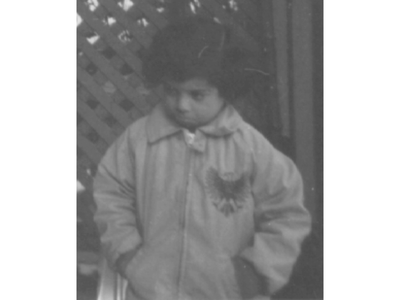
Read image and display it.
ref = imread('pout.tif');
imshow(ref)
Create another image by adding noise to a copy of the reference image.
A = imnoise(ref,'salt & pepper', 0.02);
imshow(A)
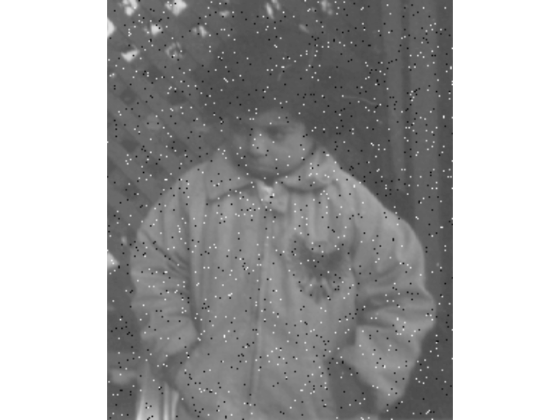
Calculate mean-squared error between the two images.
err = immse(A, ref);
fprintf('n The mean-squared error is %0.4fn', err);
The mean-squared error is 353.7631
Input Arguments
collapse all
X — Input array
numeric array
Input array, specified as a numeric array of any dimension.
Data Types: single | double | int8 | int16 | int32 | uint8 | uint16 | uint32
Y — Input array
numeric array
Input array, specified as a numeric array of the same size and data type as
X.
Data Types: single | double | int8 | int16 | int32 | uint8 | uint16 | uint32
Output Arguments
collapse all
err — Mean-squared error
positive number
Mean-squared error, returned as a positive number. The data type of err
is double unless the input arguments are of data type
single, in which case err is of
data type single
Data Types: single | double
Extended Capabilities
C/C++ Code Generation
Generate C and C++ code using MATLAB® Coder™.
immse supports the generation of C
code (requires MATLAB®
Coder™). For more information, see Code Generation for Image Processing.
GPU Code Generation
Generate CUDA® code for NVIDIA® GPUs using GPU Coder™.
Version History
Introduced in R2014b
1. Introduction
Image Quality Assessment (IQA) is considered as a characteristic property of an image. Degradation of perceived images is measured by image quality assessment. Usually, degradation is calculated compared to an ideal image known as reference image.
Quality of image can be described technically as well as objectively to indicate the deviation from the ideal or reference model. It also relates to the subjective perception or prediction of an image [1] , such as an image of a human look.
The reduction of the quality of an image is affected by the noise. This noise depends on how it correlates with the information the viewer seeks in the image.
Visual information can have many featuring steps such as acquisition, enhancement, compression or transmission. Some information provided by the features of an image can be distorted after completion of the processing. That’s why the quality should be evaluated by the human view perceptron [2] . Practically, there are two kinds of evaluation: subjective and objective. Subjective evaluation is time-consuming and also expensive to implement. Afterwards, the objective image quality metrics are developed on the basis of different aspects.
There are several techniques and metrics available to be used for objective image quality assessment. These techniques are grouped into two categories based on the availability of a reference image [3] . The categories are as follows:
1) Full-Reference (FR) approaches: The FR approaches focus on the assessment of the quality of a test image in comparison with a reference image. This reference image is considered as the perfect quality image that means the ground truth. For example, an original image is compared to the JPEG-compressed image [3] [4] .
2) No-Reference (NR) approach: The NR metrics focus on the assessment of the quality of a test image only. No reference image is used in this method [3] .
Image quality metrics are also categorized to measure a specific type of degradation such as blurring, blocking, ringing, or all possible distortions of signals.
The mean squared error (MSE) is the most widely used and also the simplest full reference metric which is calculated by the squared intensity differences of distorted and reference image pixels and averaging them with the peak signal-to-noise ratio (PSNR) of the related quantity [5] .
Image quality assessment metrics such as MSE, PSNR are mostly applicable as they are simple to calculate, clear in physical meanings, and also convenient to implement mathematically in the optimization context. But they are sometimes very mismatched to perceive visual quality and also are not normalized in representation. With this view, researchers have taken-into account, two normalized reference methods to give structural and feature similarities. Structured similarity indexing method (SSIM) gives normalized mean value of structural similarity between the two images and feature similarity indexing method (FSIM) gives normalized mean value of feature similarity between the two images. All these are full-reference image quality measurement metrics.
In this paper, we compare the FSIM, SSIM, MSE and PSNR values between the two images (an original and a recovered image) from denoising for different noise concentrations.
2. Quality Measurement Technique
There are so many image quality techniques largely used to evaluate and assess the quality of images such as MSE (Mean Square Error), UIQI (Universal Image Quality Index), PSNR (Peak Signal to Noise Ratio), SSIM (Structured Similarity Index Method), HVS (Human Vision System), FSIM (Feature Similarity Index Method), etc. In this paper, we have worked on SSIM, FSIM, MSE and PSNR methods to find their suitability.
2.1. MSE (Mean Square Error)
MSE is the most common estimator of image quality measurement metric. It is a full reference metric and the values closer to zero are the better.
It is the second moment of the error. The variance of the estimator and its bias are both incorporated with mean squared error. The MSE is the variance of the estimator in case of unbiased estimator. It has the same units of measurement as the square of the quantity being calculated like as variance. The MSE introduces the Root-Mean-Square Error (RMSE) or Root-Mean-Square Deviation (RMSD) and often referred to as standard deviation of the variance.
The MSE can also be said the Mean Squared Deviation (MSD) of an estimator. Estimator is referred as the procedure for measuring an unobserved quantity of image. The MSE or MSD measures the average of the square of the errors. The error is the difference between the estimator and estimated outcome. It is a function of risk, considering the expected value of the squared error loss or quadratic loss.
Mean Squared Error (MSE) between two images such as
g
(
x
,
y
)
and
g
^
(
x
,
y
)
is defined as [6]
MSE
=
1
M
N
∑
n
=
0
M
∑
m
=
1
N
[
g
^
(
n
,
m
)
−
g
(
n
,
m
)
]
2
(1)
From Equation (1), we can see that MSE is a representation of absolute error.
2.2. RMSE (Root Mean Square Error)
Root Mean square Error is another type of error measuring technique used very commonly to measure the differences between the predicted value by an estimator and the actual value. It evaluates the error magnitude. It is a perfect measure of accuracy which is used to perform the differences of forecasting errors from the different estimators for a definite variable [7] .
Let us suppose that
θ
^
be an estimator with respect to a given estimated parameter θ, the Root Mean Square Error is actually the square root of the Mean Square Error as
RMSE
(
θ
^
)
=
MSE
(
θ
^
)
(2)
2.3. PSNR (Peak Signal to Noise Ratio)
PSNR is used to calculate the ratio between the maximum possible signal power and the power of the distorting noise which affects the quality of its representation. This ratio between two images is computed in decibel form. The PSNR is usually calculated as the logarithm term of decibel scale because of the signals having a very wide dynamic range. This dynamic range varies between the largest and the smallest possible values which are changeable by their quality.
The Peak signal-to-noise ratio is the most commonly used quality assessment technique to measure the quality of reconstruction of lossy image compression codecs. The signal is considered as the original data and the noise is the error yielded by the compression or distortion. The PSNR is the approximate estimation to human perception of reconstruction quality compared to the compression codecs.
In image and video compression quality degradation, the PSNR value varies from 30 to 50 dB for 8-bit data representation and from 60 to 80 dB for 16-bit data. In wireless transmission, accepted range of quality loss is approximately 20 — 25 dB [8] .
PSNR is expressed as:
PSNR
=
10
log
10
(
peakval
2
)
/
MSE
(3)
Here, peakval (Peak Value) is the maximal in the image data. If it is an 8-bit unsigned integer data type, the peakval is 255 [8] . From Equation (3), we can see that it is a representation of absolute error in dB.
2.4. Structure Similarity Index Method (SSIM)
Structural Similarity Index Method is a perception based model. In this method, image degradation is considered as the change of perception in structural information. It also collaborates some other important perception based fact such as luminance masking, contrast masking, etc. The term structural information emphasizes about the strongly inter-dependant pixels or spatially closed pixels. These strongly inter-dependant pixels refer some more important information about the visual objects in image domain. Luminace masking is a term where the distortion part of an image is less visible in the edges of an image. On the other hand contrast masking is a term where distortions are also less visible in the texture of an image. SSIM estimates the perceived quality of images and videos. It measures the similarity between two images: the original and the recovered.
There is an advanced version of SSIM called Multi Scale Structural Similarity Index Method (MS-SSIM) that evaluates various structural similarity images at different image scale [9] . In MS-SSIM, two images are compared to the scale of same size and resolutions. As Like as SSIM, change in luminance, contrast and structure are considered to calculate multi scale structural similarity between two images [10] . Sometimes it gives better performance over SSIM on different subjective image and video databases.
Another version of SSIM, called a three-component SSIM (3-SSIM) that corresponds to the fact: human visual system observes the differences more accurately in textured regions than the smooth regions. This 3-component SSIM model was proposed by Ran and Farvardin [11] where an image is disintegrated into three important properties such as edge, texture and smooth region. The resulting metric is calculated as a weighted average of structural similarity for these three categories. The proposed weight measuring estimations are 0.5 for edges, 0.25 for texture and 0.25 for smooth regions. It can also be mentioned that a 1/0/0 weight measurement influences the results to be closer to the subjective ratings. This can be implied that, no textures or smooth regions rather edge regions play a dominant role in perception of image quality [11] .
2.5. DSSIM (Structural Dissimilarity)
There is another distance metric referred as Structural Dissimilarity (DSSIM) deduced from the Structural Similarity (SSIM) can be expressed as:
DSSIM
(
x
,
y
)
=
1
−
SSIM
(
x
,
y
)
2
(4)
The SSIM index method, a quality measurement metric is calculated based on the computation of three major aspects termed as luminance, contrast and structural or correlation term. This index is a combination of multiplication of these three aspects [12] .
Structural Similarity Index Method can be expressed through these three terms as:
SSIM
(
x
,
y
)
=
[
l
(
x
,
y
)
]
α
⋅
[
c
(
x
,
y
)
]
β
⋅
[
s
(
x
,
y
)
]
γ
(5)
Here, l is the luminance (used to compare the brightness between two images), c is the contrast (used to differ the ranges between the brightest and darkest region of two images) and s is the structure (used to compare the local luminance pattern between two images to find the similarity and dissimilarity of the images) and α, β and γ are the positive constants [13] .
Again luminance, contrast and structure of an image can be expressed separately as:
l
(
x
,
y
)
=
2
μ
x
μ
y
+
C
1
μ
x
2
+
μ
y
2
+
C
1
(6)
c
(
x
,
y
)
=
2
σ
x
σ
y
+
C
2
σ
x
2
+
σ
y
2
+
C
2
(7)
s
(
x
,
y
)
=
σ
x
y
+
C
3
σ
x
σ
y
+
C
3
(8)
where
μ
x
and
μ
y
are the local means,
σ
x
and
σ
y
are the standard deviations and
σ
x
y
is the cross-covariance for images x and y sequentially. If
α
=
β
=
γ
=
1
, then the index is simplified as the following form using Equations (6)-(8):
SSIM
(
x
,
y
)
=
(
2
μ
x
μ
y
+
C
1
)
(
2
σ
x
σ
y
+
C
2
)
(
μ
x
2
+
μ
y
2
+
C
1
)
(
σ
x
2
+
σ
y
2
+
C
2
)
(9)
From Equation (9) we can see that FSIM is in normalized scale (values between 0 to 1). We can also express it in dB scale as 10log10[SSIM(x, y)].
2.6. Features Similarity Index Matrix (FSIM)
Feature Similarity Index Method maps the features and measures the similarities between two images. To describe FSIM we need to describe two criteria more clearly. They are: Phase Congruency (PC) and Gradient Magnitude (GM).
Phase Congruency (PC): A new method for detecting image features is phase congruency. One of the important characteristics of phase congruency is that it is invariant to light variation in images. Besides, it is also able to detect more some interesting features. It stresses on the features of the image in the domain frequency. Phase congruency is invariant to contrast.
Gradient magnitude (GM): The computation of image gradient is a very traditional topic in the digital image processing. Convolution masks used to express the operators of the gradient. There are many convolutional masks to measure the gradients. If f(x) is an image and Gx, Gy of its horizontal and vertical gradients, respectively. Then the gradient magnitude of f(x) can be defined as [13]
G
x
2
+
G
y
2
(10)
In this paper we are going to calculate the similarity between two images to assess the quality of images. Let two images are f1 (test image) and f2 (reference image) and their phase congruency can be denoted by PC1 and PC2, respectively. The Phase Congruency (PC) maps extracted from two images f1 and f2 and the Magnitude Gradient (GM) maps G1 and G2 extracted from the two images too. FSIM can be defined and calculated based on PC1, PC2, G1 and G2. At first, we can calculate the similarity of these two images as
S
P
C
=
2
P
C
1
P
C
2
+
T
1
P
C
1
2
+
P
C
2
2
+
T
1
(11)
where T1 is a positive constant which increases the stability of Spc. Practically T1 can be calculated based on the PC values. The above equation describes the measurement to determine the similarity of two positive real numbers and its range is within 0 to 1.
Similarly, we can calculate the similarity from G1 and G2 as
S
G
=
2
G
1
G
2
+
T
2
G
1
2
+
G
2
2
+
T
2
(12)
where T2 is a positive constant which depends on the dynamic range of gradient magnitude values. In this paper, both T1 and T2 are constant so that the FSIM can be conveniently used.
Now
S
P
C
and
S
G
are combined together to calculate the similarity
S
L
of f1 and f2.
S
l
can be defined as
S
L
(
x
)
=
[
S
P
C
(
x
)
]
α
⋅
[
S
G
(
x
)
]
β
(13)
where the parameters α and β are used to adjust the relative importance of PC and GM features. In this paper, we set α = β =1 for convenience. From Equations (11) to (13), it is evident that FSIM is normalized (values between 0 to 1).
3. Experimental Results and Discussions
We used three benchmark images (Lena, Barbara, Cameraman) and then used Gaussian noise of different concentrations (noise variances). For all noise variances the mean is taken as 1.0. Then we applied Gaussian convolutional mask for denoising. The original, noisy and denoised images are shown in Figure 1, Figure 2 and Figure 3 for noise variances 0.2, 0.4 and 0.6, respectively.

Figure 1. ((a), (d), (g)) are three bench mark original images; ((b), (e), (h)) are the corresponding noisy images with noise variance 0.2; ((c), (f), (i)) are the corresponding denoised images. Here, the noise level is 0.4. The MSE, PSNR, SSIM and FSIM value of two images (the original and the recovered image) are listed in Table 1.

Figure 2. ((a), (d), (g)) are three bench mark original images; ((b), (e), (h)) are the corresponding noisy images with noise variance 0.4; ((c), (f), (i)) are the corresponding denoised images Here, the noise level is 0.4. The MSE, PSNR, SSIM and FSIM value of two images (the original and the recovered image) are listed in Table 1.
After denoising, we estimated the quality of the denoised (restored/recoverd) images by using FSIM, SSIM, PSNR and MSE metrics. The summary of quality matrices calculation is shown in Table 1. From this table, we can see that all metrics have given almost consistent results. However, from representation perspective, SSIM and FSIM are normalized, but MSE and PSNR are not. So, SSIM and FSIM can be treated more understandable than the MSE and PSNR. This is because, MSE and PSNR are absolute errors, however, SSIM and FSIM are giving perception and saliency-based errors. If noise level is increasing, then the

Figure 3. ((a), (d), (g)) are three bench mark original images; ((b), (e), (h)) are the corresponding noisy images with noise variance 0.6; ((c), (f), (i)) are the corresponding denoised images Here, the noise level is 0.6. The MSE, PSNR, SSIM and FSIM value of two images (the original and the recovered image) are listed in Table 1.
recovery quality of output image is also deteriorating.
4. Conclusion
Image Quality Assessment plays a very significant role in digital image processing applications. The metrics (MSE, PSNR, SSIM and FSIM) are applied in this paper to get the best quality metric. We have done simulating experiments using Gaussian noise through Gaussian filtering technique. The obtained image quality has been judged on applying the above metrics. We found consistent

Table 1. Error deduction summary for different image quality metrics (MSE, PSNR, SSIM, FSIM).
results for all the metrics. However, from representation perspective, SSIM and FSIM are normalized, but MSE and PSNR are not. So, SSIM and FSIM can be treated more understandable than the MSE and PSNR. This is due to the fact that MSE and PSNR are absolute errors, however, SSIM and FSIM are giving perception and saliency-based errors. If noise level is increasing, then the recovery quality of output image is also deteriorating. So, we can conclude that SSIM and SSIM are comparatively better than MSE and PSNR metrics from human visual perspective.