In statistics, the mean squared error (MSE)[1] or mean squared deviation (MSD) of an estimator (of a procedure for estimating an unobserved quantity) measures the average of the squares of the errors—that is, the average squared difference between the estimated values and the actual value. MSE is a risk function, corresponding to the expected value of the squared error loss.[2] The fact that MSE is almost always strictly positive (and not zero) is because of randomness or because the estimator does not account for information that could produce a more accurate estimate.[3] In machine learning, specifically empirical risk minimization, MSE may refer to the empirical risk (the average loss on an observed data set), as an estimate of the true MSE (the true risk: the average loss on the actual population distribution).
The MSE is a measure of the quality of an estimator. As it is derived from the square of Euclidean distance, it is always a positive value that decreases as the error approaches zero.
The MSE is the second moment (about the origin) of the error, and thus incorporates both the variance of the estimator (how widely spread the estimates are from one data sample to another) and its bias (how far off the average estimated value is from the true value).[citation needed] For an unbiased estimator, the MSE is the variance of the estimator. Like the variance, MSE has the same units of measurement as the square of the quantity being estimated. In an analogy to standard deviation, taking the square root of MSE yields the root-mean-square error or root-mean-square deviation (RMSE or RMSD), which has the same units as the quantity being estimated; for an unbiased estimator, the RMSE is the square root of the variance, known as the standard error.
Definition and basic propertiesEdit
The MSE either assesses the quality of a predictor (i.e., a function mapping arbitrary inputs to a sample of values of some random variable), or of an estimator (i.e., a mathematical function mapping a sample of data to an estimate of a parameter of the population from which the data is sampled). The definition of an MSE differs according to whether one is describing a predictor or an estimator.
PredictorEdit
If a vector of predictions is generated from a sample of data points on all variables, and is the vector of observed values of the variable being predicted, with being the predicted values (e.g. as from a least-squares fit), then the within-sample MSE of the predictor is computed as
In other words, the MSE is the mean of the squares of the errors . This is an easily computable quantity for a particular sample (and hence is sample-dependent).
In matrix notation,
where is and is the column vector.
The MSE can also be computed on q data points that were not used in estimating the model, either because they were held back for this purpose, or because these data have been newly obtained. Within this process, known as statistical learning, the MSE is often called the test MSE,[4] and is computed as
EstimatorEdit
The MSE of an estimator with respect to an unknown parameter is defined as[1]
This definition depends on the unknown parameter, but the MSE is a priori a property of an estimator. The MSE could be a function of unknown parameters, in which case any estimator of the MSE based on estimates of these parameters would be a function of the data (and thus a random variable). If the estimator is derived as a sample statistic and is used to estimate some population parameter, then the expectation is with respect to the sampling distribution of the sample statistic.
The MSE can be written as the sum of the variance of the estimator and the squared bias of the estimator, providing a useful way to calculate the MSE and implying that in the case of unbiased estimators, the MSE and variance are equivalent.[5]
Proof of variance and bias relationshipEdit
An even shorter proof can be achieved using the well-known formula that for a random variable , . By substituting with, , we have
But in real modeling case, MSE could be described as the addition of model variance, model bias, and irreducible uncertainty (see Bias–variance tradeoff). According to the relationship, the MSE of the estimators could be simply used for the efficiency comparison, which includes the information of estimator variance and bias. This is called MSE criterion.
In regressionEdit
In regression analysis, plotting is a more natural way to view the overall trend of the whole data. The mean of the distance from each point to the predicted regression model can be calculated, and shown as the mean squared error. The squaring is critical to reduce the complexity with negative signs. To minimize MSE, the model could be more accurate, which would mean the model is closer to actual data. One example of a linear regression using this method is the least squares method—which evaluates appropriateness of linear regression model to model bivariate dataset,[6] but whose limitation is related to known distribution of the data.
The term mean squared error is sometimes used to refer to the unbiased estimate of error variance: the residual sum of squares divided by the number of degrees of freedom. This definition for a known, computed quantity differs from the above definition for the computed MSE of a predictor, in that a different denominator is used. The denominator is the sample size reduced by the number of model parameters estimated from the same data, (n−p) for p regressors or (n−p−1) if an intercept is used (see errors and residuals in statistics for more details).[7] Although the MSE (as defined in this article) is not an unbiased estimator of the error variance, it is consistent, given the consistency of the predictor.
In regression analysis, «mean squared error», often referred to as mean squared prediction error or «out-of-sample mean squared error», can also refer to the mean value of the squared deviations of the predictions from the true values, over an out-of-sample test space, generated by a model estimated over a particular sample space. This also is a known, computed quantity, and it varies by sample and by out-of-sample test space.
ExamplesEdit
MeanEdit
Suppose we have a random sample of size from a population, . Suppose the sample units were chosen with replacement. That is, the units are selected one at a time, and previously selected units are still eligible for selection for all draws. The usual estimator for the is the sample average
which has an expected value equal to the true mean (so it is unbiased) and a mean squared error of
where is the population variance.
For a Gaussian distribution, this is the best unbiased estimator (i.e., one with the lowest MSE among all unbiased estimators), but not, say, for a uniform distribution.
VarianceEdit
The usual estimator for the variance is the corrected sample variance:
This is unbiased (its expected value is ), hence also called the unbiased sample variance, and its MSE is[8]
where is the fourth central moment of the distribution or population, and is the excess kurtosis.
However, one can use other estimators for which are proportional to , and an appropriate choice can always give a lower mean squared error. If we define
then we calculate:
This is minimized when
For a Gaussian distribution, where , this means that the MSE is minimized when dividing the sum by . The minimum excess kurtosis is ,[a] which is achieved by a Bernoulli distribution with p = 1/2 (a coin flip), and the MSE is minimized for Hence regardless of the kurtosis, we get a «better» estimate (in the sense of having a lower MSE) by scaling down the unbiased estimator a little bit; this is a simple example of a shrinkage estimator: one «shrinks» the estimator towards zero (scales down the unbiased estimator).
Further, while the corrected sample variance is the best unbiased estimator (minimum mean squared error among unbiased estimators) of variance for Gaussian distributions, if the distribution is not Gaussian, then even among unbiased estimators, the best unbiased estimator of the variance may not be
Gaussian distributionEdit
The following table gives several estimators of the true parameters of the population, μ and σ2, for the Gaussian case.[9]
| True value | Estimator | Mean squared error |
|---|---|---|
| = the unbiased estimator of the population mean, | ||
| = the unbiased estimator of the population variance, | ||
| = the biased estimator of the population variance, | ||
| = the biased estimator of the population variance, |
InterpretationEdit
An MSE of zero, meaning that the estimator predicts observations of the parameter with perfect accuracy, is ideal (but typically not possible).
Values of MSE may be used for comparative purposes. Two or more statistical models may be compared using their MSEs—as a measure of how well they explain a given set of observations: An unbiased estimator (estimated from a statistical model) with the smallest variance among all unbiased estimators is the best unbiased estimator or MVUE (Minimum-Variance Unbiased Estimator).
Both analysis of variance and linear regression techniques estimate the MSE as part of the analysis and use the estimated MSE to determine the statistical significance of the factors or predictors under study. The goal of experimental design is to construct experiments in such a way that when the observations are analyzed, the MSE is close to zero relative to the magnitude of at least one of the estimated treatment effects.
In one-way analysis of variance, MSE can be calculated by the division of the sum of squared errors and the degree of freedom. Also, the f-value is the ratio of the mean squared treatment and the MSE.
MSE is also used in several stepwise regression techniques as part of the determination as to how many predictors from a candidate set to include in a model for a given set of observations.
ApplicationsEdit
- Minimizing MSE is a key criterion in selecting estimators: see minimum mean-square error. Among unbiased estimators, minimizing the MSE is equivalent to minimizing the variance, and the estimator that does this is the minimum variance unbiased estimator. However, a biased estimator may have lower MSE; see estimator bias.
- In statistical modelling the MSE can represent the difference between the actual observations and the observation values predicted by the model. In this context, it is used to determine the extent to which the model fits the data as well as whether removing some explanatory variables is possible without significantly harming the model’s predictive ability.
- In forecasting and prediction, the Brier score is a measure of forecast skill based on MSE.
Loss functionEdit
Squared error loss is one of the most widely used loss functions in statistics[citation needed], though its widespread use stems more from mathematical convenience than considerations of actual loss in applications. Carl Friedrich Gauss, who introduced the use of mean squared error, was aware of its arbitrariness and was in agreement with objections to it on these grounds.[3] The mathematical benefits of mean squared error are particularly evident in its use at analyzing the performance of linear regression, as it allows one to partition the variation in a dataset into variation explained by the model and variation explained by randomness.
CriticismEdit
The use of mean squared error without question has been criticized by the decision theorist James Berger. Mean squared error is the negative of the expected value of one specific utility function, the quadratic utility function, which may not be the appropriate utility function to use under a given set of circumstances. There are, however, some scenarios where mean squared error can serve as a good approximation to a loss function occurring naturally in an application.[10]
Like variance, mean squared error has the disadvantage of heavily weighting outliers.[11] This is a result of the squaring of each term, which effectively weights large errors more heavily than small ones. This property, undesirable in many applications, has led researchers to use alternatives such as the mean absolute error, or those based on the median.
See alsoEdit
- Bias–variance tradeoff
- Hodges’ estimator
- James–Stein estimator
- Mean percentage error
- Mean square quantization error
- Mean square weighted deviation
- Mean squared displacement
- Mean squared prediction error
- Minimum mean square error
- Minimum mean squared error estimator
- Overfitting
- Peak signal-to-noise ratio
NotesEdit
- ^ This can be proved by Jensen’s inequality as follows. The fourth central moment is an upper bound for the square of variance, so that the least value for their ratio is one, therefore, the least value for the excess kurtosis is −2, achieved, for instance, by a Bernoulli with p=1/2.
ReferencesEdit
- ^ a b «Mean Squared Error (MSE)». www.probabilitycourse.com. Retrieved 2020-09-12.
- ^ Bickel, Peter J.; Doksum, Kjell A. (2015). Mathematical Statistics: Basic Ideas and Selected Topics. Vol. I (Second ed.). p. 20.
If we use quadratic loss, our risk function is called the mean squared error (MSE) …
- ^ a b Lehmann, E. L.; Casella, George (1998). Theory of Point Estimation (2nd ed.). New York: Springer. ISBN 978-0-387-98502-2. MR 1639875.
- ^ Gareth, James; Witten, Daniela; Hastie, Trevor; Tibshirani, Rob (2021). An Introduction to Statistical Learning: with Applications in R. Springer. ISBN 978-1071614174.
- ^ Wackerly, Dennis; Mendenhall, William; Scheaffer, Richard L. (2008). Mathematical Statistics with Applications (7 ed.). Belmont, CA, USA: Thomson Higher Education. ISBN 978-0-495-38508-0.
- ^ A modern introduction to probability and statistics : understanding why and how. Dekking, Michel, 1946-. London: Springer. 2005. ISBN 978-1-85233-896-1. OCLC 262680588.
{{cite book}}: CS1 maint: others (link) - ^ Steel, R.G.D, and Torrie, J. H., Principles and Procedures of Statistics with Special Reference to the Biological Sciences., McGraw Hill, 1960, page 288.
- ^ Mood, A.; Graybill, F.; Boes, D. (1974). Introduction to the Theory of Statistics (3rd ed.). McGraw-Hill. p. 229.
- ^ DeGroot, Morris H. (1980). Probability and Statistics (2nd ed.). Addison-Wesley.
- ^ Berger, James O. (1985). «2.4.2 Certain Standard Loss Functions». Statistical Decision Theory and Bayesian Analysis (2nd ed.). New York: Springer-Verlag. p. 60. ISBN 978-0-387-96098-2. MR 0804611.
- ^ Bermejo, Sergio; Cabestany, Joan (2001). «Oriented principal component analysis for large margin classifiers». Neural Networks. 14 (10): 1447–1461. doi:10.1016/S0893-6080(01)00106-X. PMID 11771723.
В данной главе мы изучим инструмент, который позволяет анализировать ошибку алгоритма в зависимости от некоторого набора факторов, влияющих на итоговое качество его работы. Этот инструмент в литературе называется bias-variance decomposition — разложение ошибки на смещение и разброс. В разложении, на самом деле, есть и третья компонента — случайный шум в данных, но ему не посчастливилось оказаться в названии. Данное разложение оказывается полезным в некоторых теоретических исследованиях работы моделей машинного обучения, в частности, при анализе свойств ансамблевых моделей.
Некоторые картинки в тексте кликабельны. Это означает, что они были заимствованы из какого-то источника и при клике вы сможете перейти к этому источнику.
Вывод разложения bias-variance для MSE
Рассмотрим задачу регрессии с квадратичной функцией потерь. Представим также для простоты, что целевая переменная $y$ — одномерная и выражается через переменную $x$ как:
$$
y = f(x) + varepsilon,
$$
где $f$ — некоторая детерминированная функция, а $varepsilon$ — случайный шум со следующими свойствами:
$$
mathbb{E} varepsilon = 0, , mathbb{V}text{ar} varepsilon = mathbb{E} varepsilon^2 = sigma^2.
$$
В зависимости от природы данных, которые описывает эта зависимость, её представление в виде точной $f(x)$ и случайной $varepsilon$ может быть продиктовано тем, что:
-
данные на самом деле имеют случайный характер;
-
измерительный прибор не может зафиксировать целевую переменную абсолютно точно;
-
имеющихся признаков недостаточно, чтобы исчерпывающим образом описать объект, пользователя или событие.
Функция потерь на одном объекте $x$ равна
$$
MSE = (y(x) — a(x))^2
$$
Однако знание значения MSE только на одном объекте не может дать нам общего понимания того, насколько хорошо работает наш алгоритм. Какие факторы мы бы хотели учесть при оценке качества алгоритма? Например, то, что выход алгоритма на объекте $x$ зависит не только от самого этого объекта, но и от выборки $X$, на которой алгоритм обучался:
$$
X = ((x_1, y_1), ldots, (x_ell, y_ell))
$$
$$
a(x) = a(x, X)
$$
Кроме того, значение $y$ на объекте $x$ зависит не только от $x$, но и от реализации шума в этой точке:
$$
y(x) = y(x, varepsilon)
$$
Наконец, измерять качество мы бы хотели на тестовых объектах $x$ — тех, которые не встречались в обучающей выборке, а тестовых объектов у нас в большинстве случаев более одного. При включении всех вышеперечисленных источников случайности в рассмотрение логичной оценкой качества алгоритма $a$ кажется следующая величина:
$$
Q(a) = mathbb{E}_x mathbb{E}_{X, varepsilon} [y(x, varepsilon) — a(x, X)]^2
$$
Внутреннее матожидание позволяет оценить качество работы алгоритма в одной тестовой точке $x$ в зависимости от всевозможных реализаций $X$ и $varepsilon$, а внешнее матожидание усредняет это качество по всем тестовым точкам.
Замечание. Запись $mathbb{E}_{X, varepsilon}$ в общем случае обозначает взятие матожидания по совместному распределению $X$ и $varepsilon$. Однако, поскольку $X$ и $varepsilon$ независимы, она равносильна последовательному взятию матожиданий по каждой из переменных: $mathbb{E}_{X, varepsilon} = mathbb{E}_{X} mathbb{E}_{varepsilon}$, но последний вариант выглядит несколько более громоздко.
Попробуем представить выражение для $Q(a)$ в более удобном для анализа виде. Начнём с внутреннего матожидания:
$$
mathbb{E}_{X, varepsilon} [y(x, varepsilon) — a(x, X)]^2 = mathbb{E}_{X, varepsilon}[f(x) + varepsilon — a(x, X)]^2 =
$$
$$
= mathbb{E}_{X, varepsilon} [ underbrace{(f(x) — a(x, X))^2}_{text{не зависит от $varepsilon$}} +
underbrace{2 varepsilon cdot (f(x) — a(x, X))}_{text{множители независимы}} + varepsilon^2 ] =
$$
$$
= mathbb{E}_X left[
(f(x) — a(x, X))^2
right] + 2 underbrace{mathbb{E}_varepsilon[varepsilon]}_{=0} cdot mathbb{E}_X (f(x) — a(x, X)) + mathbb{E}_varepsilon varepsilon^2 =
$$
$$
= mathbb{E}_X left[ (f(x) — a(x, X))^2 right] + sigma^2
$$
Из общего выражения для $Q(a)$ выделилась шумовая компонента $sigma^2$. Продолжим преобразования:
$$
mathbb{E}_X left[ (f(x) — a(x, X))^2 right] = mathbb{E}_X left[
(f(x) — mathbb{E}_X[a(x, X)] + mathbb{E}_X[a(x, X)] — a(x, X))^2
right] =
$$
$$
= mathbb{E}_Xunderbrace{left[
(f(x) — mathbb{E}_X[a(x, X)])^2
right]}_{text{не зависит от $X$}} + underbrace{mathbb{E}_X left[ (a(x, X) — mathbb{E}_X[a(x, X)])^2 right]}_{text{$=mathbb{V}text{ar}_X[a(x, X)]$}} +
$$
$$
+ 2 mathbb{E}_X[underbrace{(f(x) — mathbb{E}_X[a(x, X)])}_{text{не зависит от $X$}} cdot (mathbb{E}_X[a(x, X)] — a(x, X))] =
$$
$$
= (underbrace{f(x) — mathbb{E}_X[a(x, X)]}_{text{bias}_X a(x, X)})^2 + mathbb{V}text{ar}_X[a(x, X)] + 2 (f(x) — mathbb{E}_X[a(x, X)]) cdot underbrace{(mathbb{E}_X[a(x, X)] — mathbb{E}_X [a(x, X)])}_{=0} =
$$
$$
= text{bias}_X^2 a(x, X)+ mathbb{V}text{ar}_X[a(x, X)]
$$
Таким образом, итоговое выражение для $Q(a)$ примет вид
$$
Q(a) = mathbb{E}_x mathbb{E}_{X, varepsilon} [y(x, varepsilon) — a(x, X)]^2 = mathbb{E}_x text{bias}_X^2 a(x, X) + mathbb{E}_x mathbb{V}text{ar}_X[a(x, X)] + sigma^2,
$$
где
$$
text{bias}_X a(x, X) = f(x) — mathbb{E}_X[a(x, X)]
$$
— смещение предсказания алгоритма в точке $x$, усреднённого по всем возможным обучающим выборкам, относительно истинной зависимости $f$;
$$
mathbb{V}text{ar}_X[a(x, X)] = mathbb{E}_X left[ a(x, X) — mathbb{E}_X[a(x, X)] right]^2
$$
— дисперсия (разброс) предсказаний алгоритма в зависимости от обучающей выборки $X$;
$$
sigma^2 = mathbb{E}_x mathbb{E}_varepsilon[y(x, varepsilon) — f(x)]^2
$$
— неустранимый шум в данных.
Смещение показывает, насколько хорошо с помощью данного алгоритма можно приблизить истинную зависимость $f$, а разброс характеризует чувствительность алгоритма к изменениям в обучающей выборке. Например, деревья маленькой глубины будут в большинстве случаев иметь высокое смещение и низкий разброс предсказаний, так как они не могут слишком хорошо запомнить обучающую выборку. А глубокие деревья, наоборот, могут безошибочно выучить обучающую выборку и потому будут иметь высокий разброс в зависимости от выборки, однако их предсказания в среднем будут точнее. На рисунке ниже приведены возможные случаи сочетания смещения и разброса для разных моделей:
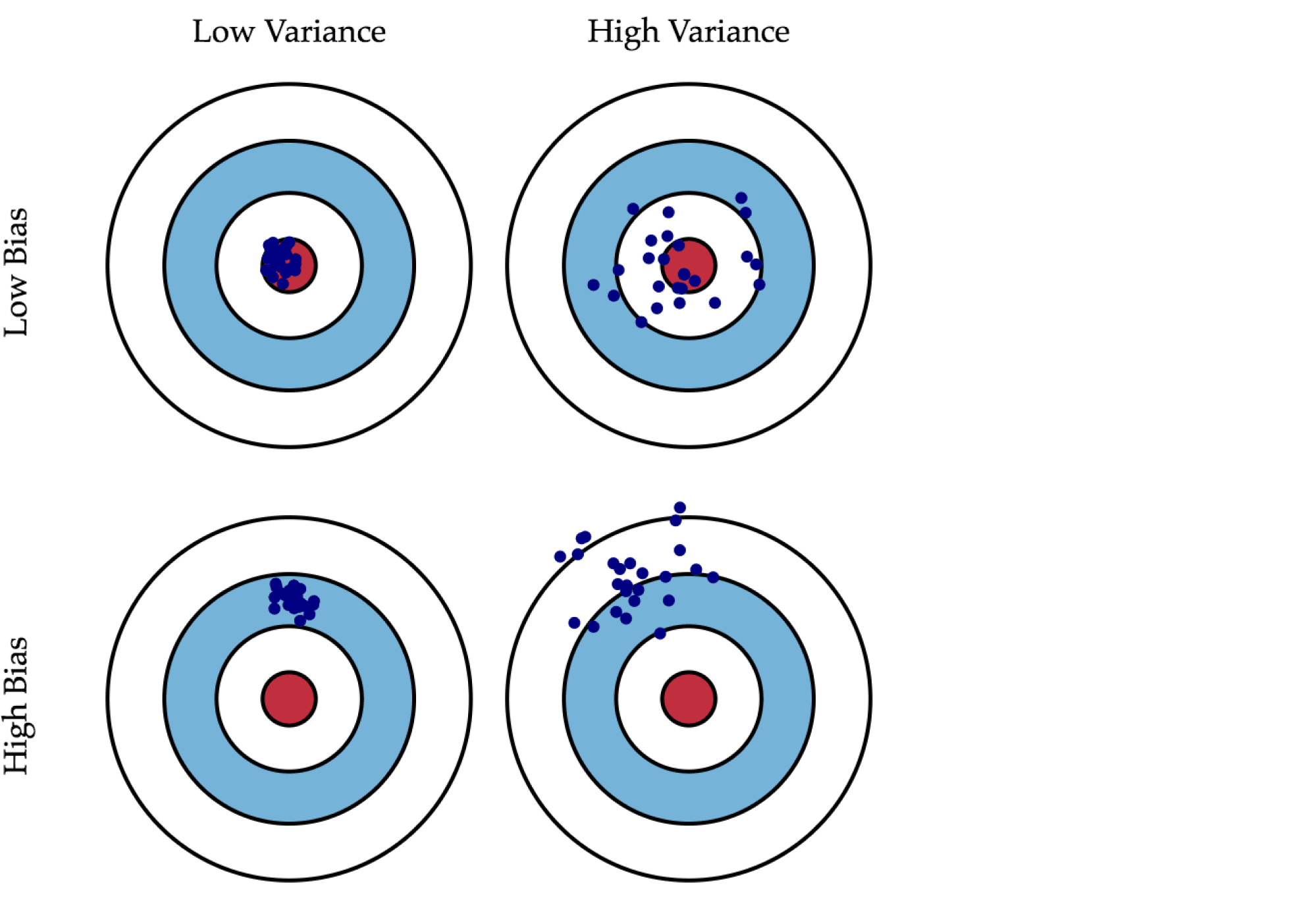
Синяя точка соответствует модели, обученной на некоторой обучающей выборке, а всего синих точек столько, сколько было обучающих выборок. Красный круг в центре области представляет ближайшую окрестность целевого значения. Большое смещение соответствует тому, что модели в среднем не попадают в цель, а при большом разбросе модели могут как делать точные предсказания, так и довольно сильно ошибаться.
Полученное нами разложение ошибки на три компоненты верно только для квадратичной функции потерь. Для других функций потерь существуют более общие формы этого разложения (Domigos, 2000, James, 2003) с похожими по смыслу компонентами. Это позволяет предполагать, что для большинства основных функций потерь имеется некоторое представление в виде смещения, разброса и шума (хоть и, возможно, не в столь простой аддитивной форме).
Пример расчёта оценок bias и variance
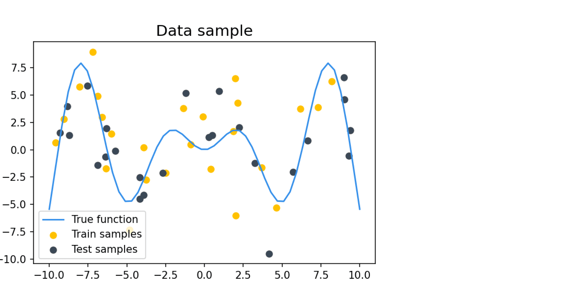
Попробуем вычислить разложение на смещение и разброс на каком-нибудь практическом примере. Наши обучающие и тестовые примеры будут состоять из зашумлённых значений целевой функции $f(x)$, где $f(x)$ определяется как
$$
f(x) = x sin x
$$
В качестве шума добавляется нормальный шум с нулевым средним и дисперсией $sigma^2$, равной во всех дальнейших примерах 9. Такое большое значение шума задано для того, чтобы задача была достаточно сложной для классификатора, который будет на этих данных учиться и тестироваться. Пример семпла из таких данных:
Посмотрим на то, как предсказания деревьев зависят от обучающих подмножеств и максимальной глубины дерева. На рисунке ниже изображены предсказания деревьев разной глубины, обученных на трёх независимых подвыборках размера 20 (каждая колонка соответствует одному подмножеству):
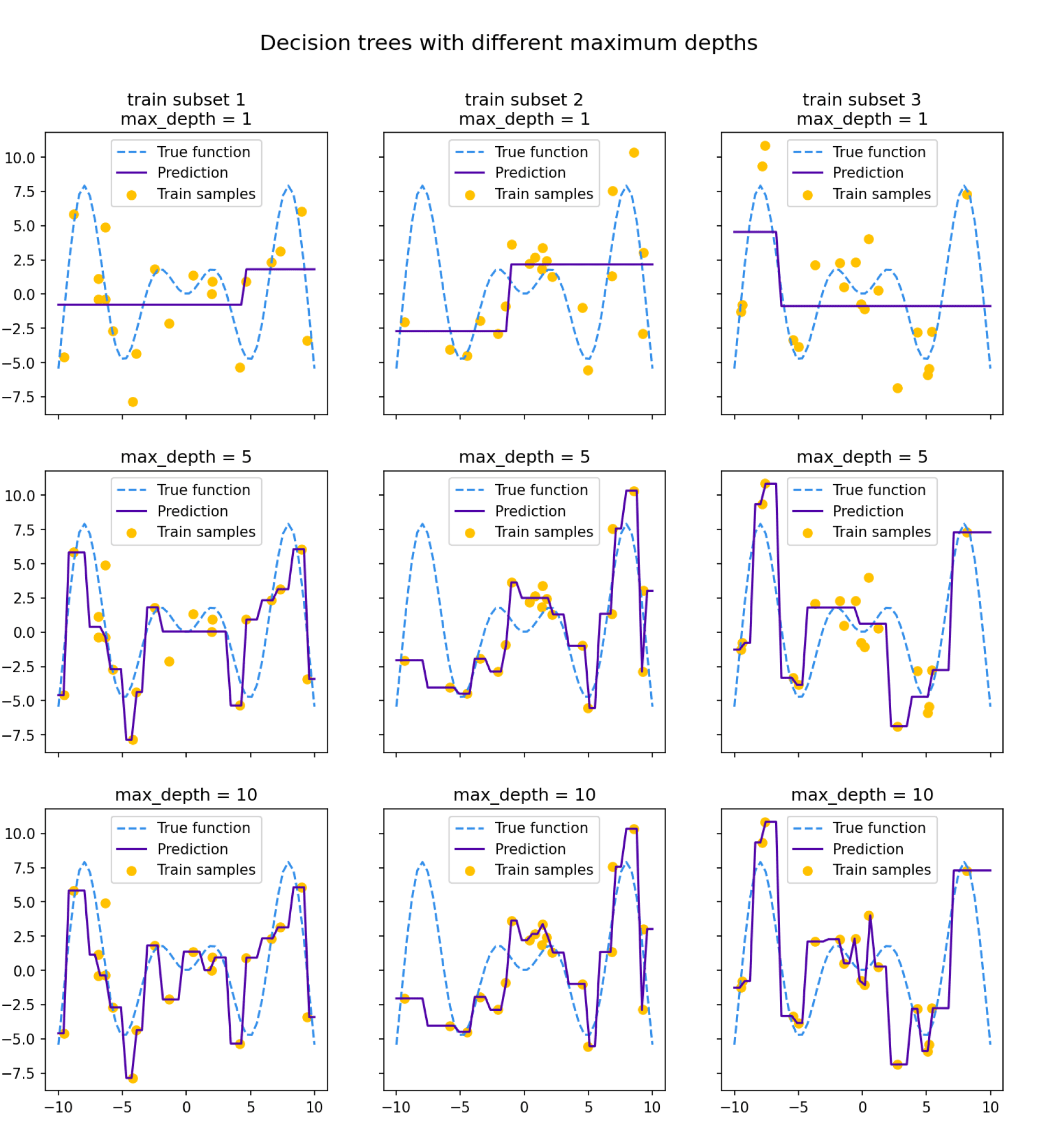
Глядя на эти рисунки, можно выдвинуть гипотезу о том, что с увеличением глубины дерева смещение алгоритма падает, а разброс в зависимости от выборки растёт. Проверим, так ли это, вычислив компоненты разложения для деревьев со значениями глубины от 1 до 15.
Для обучения деревьев насемплируем 1000 случайных подмножеств $X_{train} = (x_{train}, y_{train})$ размера 500, а для тестирования зафиксируем случайное тестовое подмножество точек $x_{test}$ также размера 500. Чтобы вычислить матожидание по $varepsilon$, нам нужно несколько экземпляров шума $varepsilon$ для тестовых лейблов:
$$
y_{test} = y(x_{test}, hat varepsilon) = f(x_{test}) + hat varepsilon
$$
Положим количество семплов случайного шума равным 300. Для фиксированных $X_{train} = (x_{train}, y_{train})$ и $X_{test} = (x_{test}, y_{test})$ квадратичная ошибка вычисляется как
$$
MSE = (y_{test} — a(x_{test}, X_{train}))^2
$$
Взяв среднее от $MSE$ по $X_{train}$, $x_{test}$ и $varepsilon$, мы получим оценку для $Q(a)$, а оценки для компонент ошибки мы можем вычислить по ранее выведенным формулам.
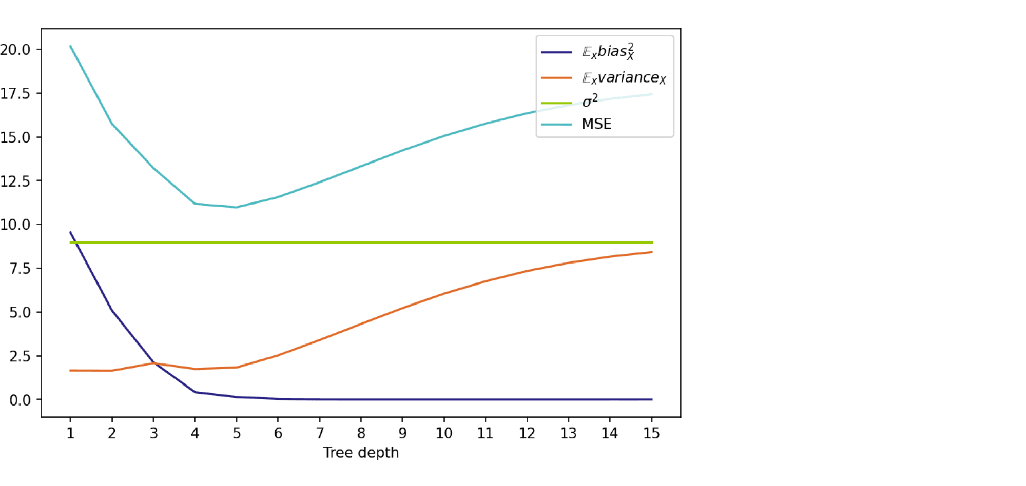
На графике ниже изображены компоненты ошибки и она сама в зависимости от глубины дерева:
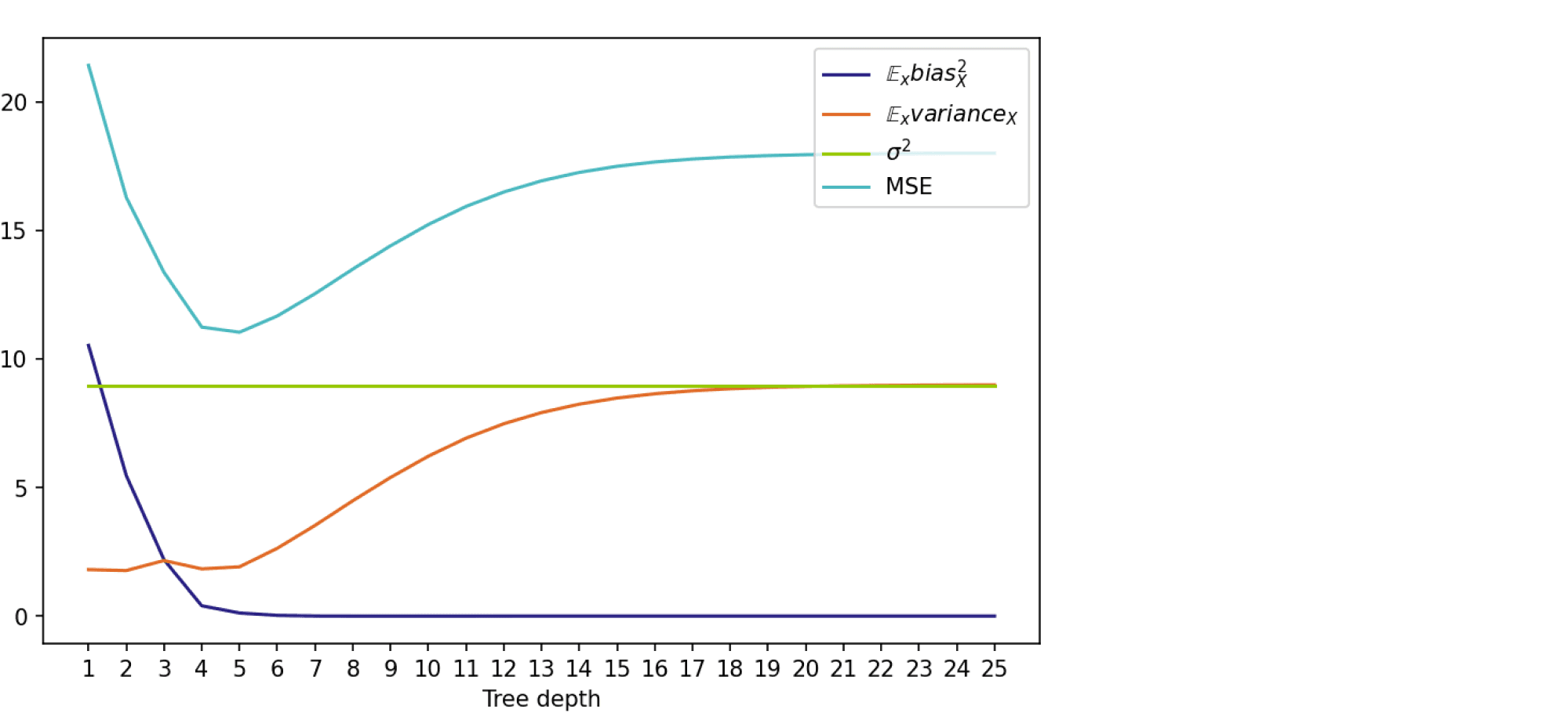
По графику видно, что гипотеза о падении смещения и росте разброса при увеличении глубины подтверждается для рассматриваемого отрезка возможных значений глубины дерева. Правда, если нарисовать график до глубины 25, можно увидеть, что разброс становится равен дисперсии случайного шума. То есть деревья слишком большой глубины начинают идеально подстраиваться под зашумлённую обучающую выборку и теряют способность к обобщению:
Код для подсчёта разложения на смещение и разброс, а также код отрисовки картинок можно найти в данном ноутбуке.
Bias-variance trade-off: в каких ситуациях он применим
В книжках и различных интернет-ресурсах часто можно увидеть следующую картинку:
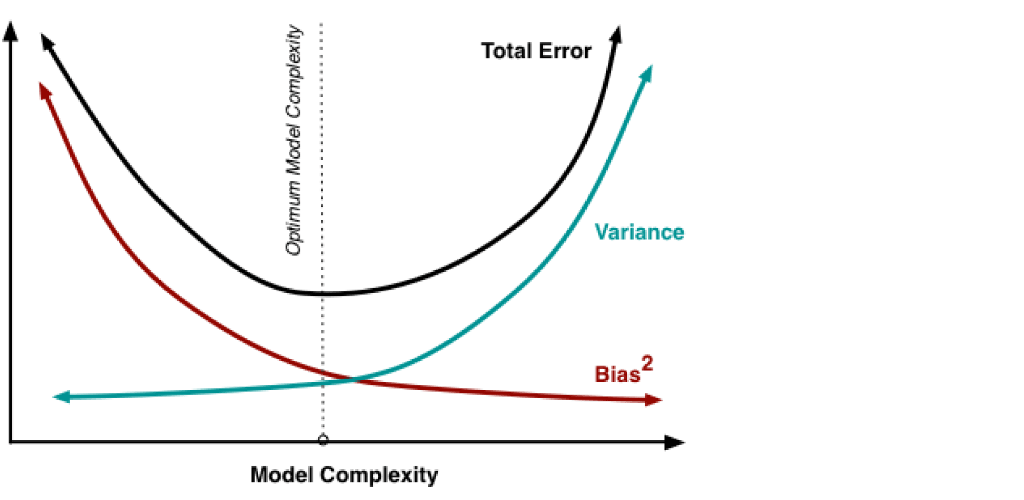
Она иллюстрирует утверждение, которое в литературе называется bias-variance trade-off: чем выше сложность обучаемой модели, тем меньше её смещение и тем больше разброс, и поэтому общая ошибка на тестовой выборке имеет вид $U$-образной кривой. С падением смещения модель всё лучше запоминает обучающую выборку, поэтому слишком сложная модель будет иметь нулевую ошибку на тренировочных данных и большую ошибку на тесте. Этот график призван показать, что существует оптимальная сложность модели, при которой соблюдается баланс между переобучением и недообучением и ошибка при этом минимальна.
Существует достаточное количество подтверждений bias-variance trade-off для непараметрических моделей. Например, его можно наблюдать для метода $k$ ближайших соседей при росте $k$ и для ядерной регрессии при увеличении ширины окна $sigma$ (Geman et al., 1992):
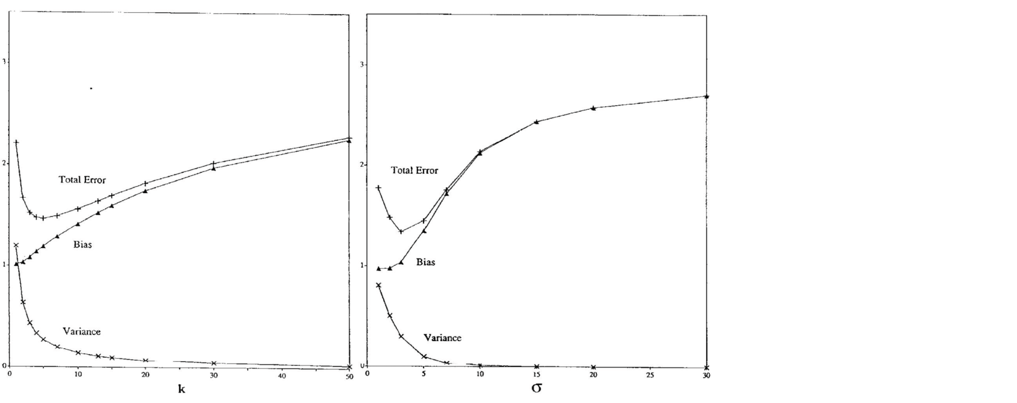
Чем больше соседей учитывает $k$-NN, тем менее изменчивым становится его предсказание, и аналогично для ядерной регрессии, из-за чего сложность этих моделей в некотором смысле убывает с ростом $k$ и $sigma$. Поэтому традиционный график bias-variance trade-off здесь симметрично отражён по оси $x$.
Однако, как показывают последние исследования, непременное возрастание разброса при убывании смещения не является абсолютно истинным предположением. Например, для нейронных сетей с ростом их сложности может происходить снижение и разброса, и смещения. Одна из наиболее известных статей на эту тему — статья Белкина и др. (Belkin et al., 2019), в которой, в частности, была предложена следующая иллюстрация:
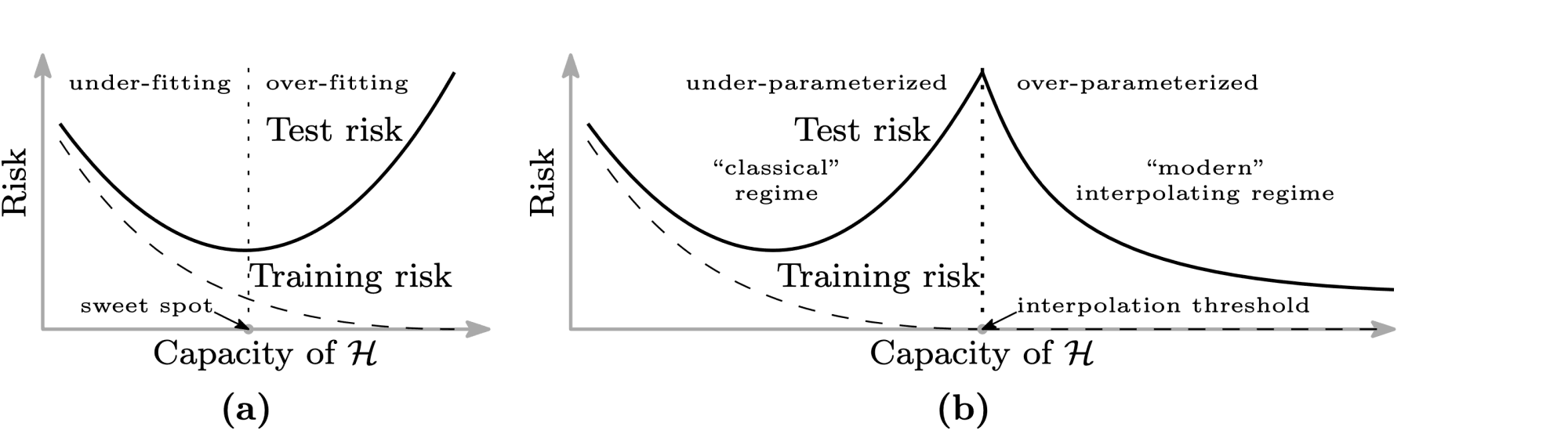
Слева — классический bias-variance trade-off: убывающая часть кривой соответствует недообученной модели, а возрастающая — переобученной. А на правой картинке — график, называемый в статье double descent risk curve. На нём изображена эмпирически наблюдаемая авторами зависимость тестовой ошибки нейросетей от мощности множества входящих в них параметров ($mathcal H$). Этот график разделён на две части пунктирной линией, которую авторы называют interpolation threshold. Эта линия соответствует точке, в которой в нейросети стало достаточно параметров, чтобы без особых усилий почти идеально запомнить всю обучающую выборку. Часть до достижения interpolation threshold соответствует «классическому» режиму обучения моделей: когда у модели недостаточно параметров, чтобы сохранить обобщающую способность при почти полном запоминании обучающей выборки. А часть после достижения interpolation threshold соответствует «современным» возможностям обучения моделей с огромным числом параметров. На этой части графика ошибка монотонно убывает с ростом количества параметров у нейросети. Авторы также наблюдают похожее поведение и для «древесных» моделей: Random Forest и бустинга над решающими деревьями. Для них эффект проявляется при одновременном росте глубины и числа входящих в ансамбль деревьев.
В качестве вывода к этому разделу хочется сформулировать два основных тезиса:
- Bias-variance trade-off нельзя считать непреложной истиной, выполняющейся для всех моделей и обучающих данных.
- Разложение на смещение и разброс не влечёт немедленного выполнения bias-variance trade-off и остаётся верным и для случая, когда все компоненты ошибки (кроме неустранимого шума) убывают одновременно. Этот факт может оказаться незамеченным из-за того, что в учебных пособиях часто разговор о разложении дополняется иллюстрацией с $U$-образной кривой, благодаря чему в сознании эти два факта могут слиться в один.
Список литературы
- Блог-пост про bias-variance от Йоргоса Папахристудиса
- Блог-пост про bias-variance от Скотта Фортмана-Роу
- Статьи от Домингоса (2000) и Джеймса (2003) про обобщённые формы bias-variance decomposition
- Блог-пост от Брейди Нила про необходимость пересмотра традиционного взгляда на bias-variance trade-off
- Статья Гемана и др. (1992), в которой была впервые предложена концепция bias-variance trade-off
- Статья Белкина и др. (2019), в которой был предложен double-descent curve
In this post we’re going to take a deeper look at Mean Squared Error. Despite the relatively simple nature of this metric, it contains a surprising amount of insight into modeling. By breaking down Mean Squared Error into bias and variance, we’ll get a better sense of how models work and ways in which they can fail to perform. We’ll also find that baked into the definition of this metric is the idea that there is always some irreducible uncertainty that we can never quite get rid of.
A quick explanation of bias
The primary mathematical tools we’ll be using are expectation, variance and bias. We’ve talked about expectation and variance quite a bit on this blog, but we need to introduce the idea of bias. Bias is used when we have an estimator, (hat{y}), that is used to predict another value (y). For example you might want to predict the rainfall, in inches, for your city in a given year. The bias is the average difference between that estimator and true value. Mathematically we just write bias as:
$$E[hat{y}-y]$$
Note that unlike variance, bias can be either positive or negative. If your rainfall predictions for your city had a bias of 0, it means that you’re just as likely to predict too much rain as to predict too little. If your bias was positive it means that you tend to predict more rain than actually occurs. Likewise, negative bias means that you underpredict. However, bias alone says little about how correct you are. Your forecasts could always be wildly wrong, but if you predict a drought during the rainiest year and predict floods during the driest then your bias can still be 0.
What is Modeling?
Before we dive too deeply into our problem, we want to be very clear about what we’re even trying to do whenever we model data. Even if you’re an expert in machine learning or scientific modeling, it’s always worth it to take a moment to make sure everything is clear. Whether we’re just making a random guess, building a deep neural network, or formulating a mathematical model of the physical universe, anytime we’re modeling we are attempting to understand some process in nature. Mathematically we describe this process as an unknown (and perhaps unknowable) function (f). This could be the process of curing meat, the complexity of a game of basketball, the rotation of the planets, etc.
Describing the world
To understand this process we have some information about how the world works and we know what outcome we expect from the process. The information about the world is our data and we use the variable (x) to denote this. It is easy to imagine (x) as just a single value, but it could be a vector of values, a matrix a values or something even more complex. And we know that this information about the world produces a result (y). Again we can think of (y) as a single value, but it can also be more complex values. This gives us our basic understanding of things, and we have the following equation:
$$y = f(x)$$
So (x) could the height a object is dropped, (f) could be the effects of gravity and the atmosphere on the object and (y) the time it takes to hit the ground. However, one very important thing is missing from this description of how things work. Clearly if you drop an object and time it, you will get slightly different observations, especially if you drop different objects. We consider this the «noise» in this process and we note that with a variable (epsilon) (lower case «epsilon» for those unfamiliar). Now we have this equation:
$$y = f(x) + epsilon$$
The (epsilon ) value is considered to be normally distributed with some standard deviation (sigma) and a mean of 0. We’ll note this as (mathcal{N}(mu=0,sigma)). This means that a negative and a positive impact from this noise are considered equally likely, and that small errors are much more likely than extreme ones.
Our model
This equation is just for how the world actually works given (x) that we know and (y) that we observe. However, we don’t really know how the world works so we have to make models. A model, in it’s most general form, is simply some other function (hat{f}) that takes (x) and should approximate (y). Mathematically we might say:
$$hat{f}(x) approx y$$
However it’s useful to expand out (y) into (f(x) + epsilon). This helps us see that (hat{f}) is not approximating (f), that is our natural process, directly.
$$hat{f}(x_i) approx f(x_i) + epsilon_i $$
Instead we have to remember that (hat{f}) models (y) which includes our noise. In practical modeling and machine learning this is an important thing to remember. If our noise term is very large, it can be difficult or even impossible to meaningfully capture the behavior of (f) itself.
Measuring the success of our model with Mean Squared Error.
Once we have implemented a model we need to check how well it preforms. In machine learning we typically split of our data into training and testing data, but you can also imagine a scientist building a model on past experiments or an economist making a model based on economic theories. In whichever case, we want to test our the model and measure it’s success. When we do this we have a new set of data, (x) with each values in that set being indexed by value so we label them all (x_i). To evaluate the model we need to compare this to some (y_i). The most common way to do this for real valued data is to use Mean Squared Error (MSE). MSE is exactly what it sounds like:
— We take the error (i.e. difference from (hat{f}(x_i)) and (y))
— Square this value (making negative in positive the same, and greater error gets more severe penalty)
— Then we take the average (mean) of these results.
Mathematically we express this as:
$$MSE = frac{1}{n}Sigma_{i=1}^n (y -hat{f}(x_i))^2 $$
Of course the mean of our squared error is also the same thing as the expectation of our squared error so we can go ahead and simplify this a bit:
$$MSE=E[(y-hat{f}(x))^2]$$
It’s worth noting that if our model simply predicted the mean of (y), (mu_y) for every answer, then our MSE is the same as the variance of (y), since one way we can define variance is as (E[(y-mu)^2])
Unpacking Mean Squared Error
Already MSE has some useful properties that are similar to the general properties we explored when we discussed why we square values for variance. However, even more interesting is that inside this relatively simple equation are hidden the calculations of bias and variance for our model! To find these we need to start by expanding our MSE a bit more. We’ll start by replacing (y) with (f(x) + epsilon):
$$MSE = E[(f(x)+ epsilon — hat{f}(x))^2]$$
Before moving on there is one rule of expectation we need to know so that we can manipulate this a bit better:
$$E[X+Y] = E[X] + E[Y]$$
That is, adding two random variables and computing their expectation is the same as computing the expectation of each random variable and then computing that. Of course, we can’t use this on our equation yet because all of the added terms are squared. To do anything more interesting we need to expand this out fully:
$$MSE = E[(f(x)+ epsilon — hat{f}(x))^2] =E[(f(x)+ epsilon — hat{f}(x))cdot (f(x)+ epsilon — hat{f}(x))] = ldots $$
$$E[-2f(x)hat{f}(x) + f(x)^2 + 2epsilon f(x) + hat{f}(x)^2 — 2epsilon hat{f}(x) + epsilon^2]$$
Now this looks like a mess, but let’s start pulling this apart in terms of expectations of each section were adding or subtracting.
At the end we have (epsilon^2). We know that this our noise which we already stated is normally distributed with a mean, (mu=0), and an unknown standard deviation of (sigma). Recall that (sigma^2 = text{Variance}). The definition of Variance is:
$$E[X^2] — E[X]^2$$
So the variance for our (epsilon) is:
$$Var(epsilon) = sigma^2 = E[epsilon^2] — E[epsilon]^2$$
But we can do a neat trick here! We just said that (epsilon ) is sampled from a Normal distribution with mean of 0, and the mean is the exact same thing as the expectation so:
$$E[epsilon]^2 = mu^2 = 0^2 = 0$$
And because of this we know that:
$$E[epsilon^2] = sigma^2 $$
We can use this to pull out the (epsilon^2) term from our MSE definition:
$$MSE = sigma^2 + E[-2f(x)hat{f}(x) + f(x)^2 + 2epsilon f(x) + hat{f}(x)^2 — 2epsilon hat{f}(x)]$$
Which still looks pretty gross! However, if we pull out all the remaining terms with (epsilon ) in them we can clean this up very easily:
$$MSE = sigma^2 + E[2epsilon f(x)- 2epsilon hat{f}(x)] + E[-2f(x)hat{f}(x) + f(x)^2 + hat{f}(x)^2]$$
Again, we know that the expected value of (epsilon ) is 0, so all the terms in (E[2epsilon f(x)- 2epsilon hat{f}(x)]) will end up a 0 in the long run! Now we’ve cleaned up quite a bit:
$$MSE = sigma^2 + E[-2f(x)hat{f}(x)+f(x)^2 + hat{f}(x)^2]$$
And here we see that one of the terms in our MSE reduced to (sigma^2), or the variance in the noise in our process.
A note on noise variance
It is important to stress here how important this insight is. The variance of the noise in our data is an irreducible part of our MSE. No matter how clever our model is, we can never reduce our MSE to being less than the variance related to the noise. It’s also worthwhile thinking about what «noise» is. In orthodox statistics we often think of noise as just some randomness added to the data, but as a Bayesian I can’t quite swallow this view. Randomness isn’t a statement about data, it’s a statement about our state of knowledge. A better interpretation is that noise represents the unknown in our view of the world. Part of it may be simply measurement error. Any equipment measuring data has limitations. But, and this is very important, it can also account for limitations in our (x) to fully capture all the information needed to adequately explain (y). If you are trying to predict the temperature in NYC from just the atmospheric CO2 levels, there’s still far to much unknown in your model.
Model variance and bias
So now that we’ve extracted out the noise variance, we still have a bit of work to do. Luckily we can simplify the inner term of the remaining expectation quite a bit:
$$-2f(x)hat{f}(x)+f(x)^2 + hat{f}(x)^2 = (f(x)-hat{f}(x))^2 $$
With that simplification we’re now left with:
$$MSE = sigma^2 + E[(f(x)-hat{f}(x))^2]$$
Now we need to do one more transformation that is really exciting! We just defined
$$Var(X) = E[X^2] — E[X]^2$$
Which means that:
$$Var(f(x)-hat{f}(x)) = E[(f(x)-hat{f}(x))^2] — E[f(x)-hat{f}(x)]^2$$
A simple reordering of these terms solves this for our (E[(f(x)-hat{f}(x))^2])):
$$E[(f(x)-hat{f}(x))^2]=Var(f(x)-hat{f}(x)) + E[f(x)-hat{f}(x)]^2$$
And now we get a much more interesting formulation of MSE:
$$MSE = sigma^2 + Var(f(x)-hat{f}(x)) + E[f(x) — hat{f}(x)]^2$$
And here we see two remarkable terms just pop out! The first, (Var(f(x)-hat{f}(x))) is, quite literally, the variance in our predictions from the true output of our process. Notice that even though we can’t differentiate (f(x)) and (epsilon), and our model cannot either, baked in to MSE is the true variance between the non-noisy process (f) and (hat{f}). The second term that pops out is (E[f(x) — hat{f}(x)]^2), this is just the bias squared. Remember that unlike variance, bias can be positive or negative (depending on how the model is biased), so we would need to square this value in order to make sure it’s always positive.
With MSE unpacked we can see that Mean Squared Error is quite literally:
$$text{Mean Squared Error}=text{Model Variance} + text{Model Bias}^2 + text{Irreducible Uncertainty}$$
Simulating Bias and Variance
It turns out that we actually need MSE is able to capture the details of bias, variance and the uncertainty in our model because *we cannot directly observe these properties ourselves*. In practice there is no way to know explicitly what (sigma^2) is for our (epsilon). This means that we cannot directly determine what the bias and variance are exactly for our model. Since (sigma^2) is constant, we do know that if we lower our MSE we must have lowered at least one of these other properties of our model.
However to understand these concepts better we can simulate a function (f) and apply our own noises sampled from a distribution with a known variance. Here is a bit of R code that will create our a (y) value from a function (f(x) = 3cdot x + 6) with (epsilon in mathcal{N}(mu=0,sigma=3) ):
We can visualize our data and see that we get what we would expect, points scattered around a straight line:
Because we know the true (f) and (sigma) we can experiment with different (hat{f}) models and see their bias and variance. Let’s start with a model that is the same as (f) except that it has a different y-intercept:
We can plot this out and see how it looks compared to our data.
As we can see, the blue line representing our model follows our data pretty closely but it systematically underestimates our values. We can go ahead and calculate the MSE for this function and, because we know what these values are, we can also calculate the bias and variance:
-
MSE: 13
-
bias: -2
-
variance: 0
So (hat{f}_1) has a negative bias because it under estimates the points more often than it over estimates them. But, compared to the true (f),it does so consistently, so therefore has 0 variance with (f). Given that we have a MSE of 13, a bias of -2 and 0 variance, we can also calculate that our (sigma^2) for our uncertainty is
$$sigma^2 = text{MSE} — (text{bias}^2 + text{variance})= 13 — (-2^2 + 0) = 9$$
Which is exactly what we would expect given that we set our (sigma) parameter to 3 when sampling our ‘e’ values.
We can come up with another model, (hat{f}_2), which simply guesses the mean of our data, which is 21.
With this simple model we get just a straight line cutting our data in half:
When we look at the MSE, bias and variance for this model we get very different results from last time:
-
MSE: 84
-
bias: 0
-
variance: 75
Given that our new model predicts the mean it shouldn’t be surprising to see that this model is has no bias since it underestimates (f(x)) just as much as it overestimates. The tradeoff here is that the variance in how the predictions differ between (hat{f_2}) and (f) is very high. And of course when we subtract out the variance from our MSE we still have the same (sigma^2=9).
For our final model,(hat{f}_3), we’ll just use R’s built-in `lm` function to build a linear model:
lm(y ~ x)When we plot this out we can see that, by minimizing the MSE, the linear model was able to recover our original (f):
Since you true function (f) is a linear model it’s not surprising that (hat{f_3}) is able to learn it. By this point you should be able to guess the results for this model:
-
MSE: 9
-
bias: 0
-
variance: 0
The MSE remains 9 because, even when we’re cheating and know the true model, we can’t learn better than the uncertainty in our data. So (sigma^2) stands as the limit for how good we can get our model to perform.
The Bias-Variance trade off
As we can see, if we want to improve our model we have to decrease either bias or variance. In practice bias and variance come up when we see how our models perform on a separate set of data than what they were trained on. In the case of testing your model out on different data than it was trained on, bias and variance can be used to diagnosis different symptoms of issues that could be wrong with your model. High bias on test data is typically caused because your model failed to find the (f) in the data and so it systematically under or over predicts. This is called «underfitting» in machine learning because you have failed to fit your model to the data.
High variance when working with test data indicates a different problem. High variance means that the predictions your model makes very greatly with what the known results should be in the test data. This high variance indicates your model has learned the training data so well that it is started to mistake the (f(x) + epsilon) for just the true (f(x)) you wanted to learn. This problem is called «overfitting», because you are fitting your model to closely to the data.
Conclusion
When we unpack and really understand Mean Squared Error we see that it is much more than just a useful error metric, but also a guide for reasoning about models. MSE allows us, in a single measurement, to capture the ideas of bias and variance in our models, as well as showing that there is some uncertainty in our models that we cannot get rid. The real magic of MSE is that it provides indirect mathematical insight about the behavior of the true process, (f), which we are never able to truly observe.
If you enjoyed this post please subscribe to keep up to date and follow @willkurt!
If you enjoyed this writing and also like programming languages, you might enjoy my book Get Programming With Haskell from Manning. Expected in July 2019 from No Starch Press is my next book Bayesian Statistics the Fun Way
Contents
- Bias and Variance of an Estimator
- Maximum Likelihood Estimation
- Example: Variance Estimator of Gaussian Data
- Example: Linear Regression
- Main Results
- Comparing linear regression and ridge regression estimators
- Bias and Variance of a Predictor (or Model)
- Setup
- Decomposition
- Discussion
- Example: Linear Regression and Ridge Regression
- Main Results
- Decomposing Bias for Linear Models
- Further areas of investigation
- Appendix
[newcommand{Noise}{mathcal{E}}
newcommand{fh}{hat{f}}
newcommand{fhR}{hat{f}^text{Ridge}}
newcommand{bff}{mathbf{f}}
newcommand{bfh}{mathbf{h}}
newcommand{bfX}{mathbf{X}}
newcommand{bfy}{mathbf{y}}
newcommand{bfZ}{mathbf{Z}}
newcommand{wh}{hat{w}}
newcommand{whR}{hat{w}^text{Ridge}}
newcommand{Th}{hat{T}}
DeclareMathOperator*{argmax}{arg,max}
DeclareMathOperator*{argmin}{arg,min}
DeclareMathOperator{Bias}{Bias}
DeclareMathOperator{var}{Var}
DeclareMathOperator{Cov}{Cov}
DeclareMathOperator{tr}{tr}]
Mean squared error (MSE) is defined in two different contexts.
- The MSE of an estimator quantifies the error of a sample statistic relative to the true population statistic.
- The MSE of a regression predictor (or model) quantifies the generalization error of that model trained on a sample of the true data distribution.
This post discusses the bias-variance decomposition for MSE in both of these contexts. To start, we prove a generic identity.
Theorem 1: For any random vector (X in R^p) and any constant vector (c in R^p),
[E[|X-c|_2^2] = trCov[X] + |E[X]-c|_2^2.]
Proof
All of the expectations and the variance are taken with respect to (P(X)). Let (mu := E[X]).
[begin{aligned}
tr Cov(X) + |mu-c|_2^2
&= sum_{i=1}^p var(X_i) + |mu-c|_2^2 \
&= sum_{i=1}^p Eleft[ (X_i — mu_i)^2 right] + |mu-c|_2^2 \
&= Eleft[sum_{i=1}^p (X_i — mu_i)^2 right] + |mu-c|_2^2 \
&= E[(X-mu)^T (X-mu)] + (mu-c)^T (mu-c) \
&= E[X^T X] underbrace{- 2 E[X]^T mu + mu^T mu + mu^T mu}_{=0} — 2 mu^T c + c^T c \
&= E[X^T X — 2 X^T c + c^T c] \
&= E[|X-c|_2^2]
end{aligned}]
We write the special case where (X) and (c) are scalars instead of vectors as a corollary.
Corollary 1: For any random variable (X in R) and any constant (c in R),
[E[(X-c)^2] = var[X] + (E[X]-c)^2.]
Bias and Variance of an Estimator
Consider a probability distribution (P_T(X)) parameterized by (T), and let (D = { x^{(i)} }_{i=1}^N) be a set of samples drawn i.i.d. from (P_T(X)). Let (Th = Th(D)) be an estimator of (T) that has variability due to the randomness of the data from which it is computed.
For example, (T) could be the mean of (P_T(X)). The sample mean (Th = frac{1}{N} sum_{i=1}^N x^{(i)}) is an estimator of (T).
For the rest of this section, we will use the abbreviation (E_T equiv E_{D sim P_T(X)}) and similarly for variance.
The mean squared error of (Th) decomposes nicely into the squared-bias and variance of (Th) by a straightforward application of Theorem 1 where (T) is constant.
[begin{aligned}
MSE(Th)
&= E_Tleft[ |Th(D) — T|_2^2 right] \
&= | E_T[Th] — T |_2^2 + trCov_T[Th] \
&= |Bias[Th]|_2^2 + trCov[Th]
end{aligned}]
Terminology for an estimator (Th):
- The standard error of a scalar estimator (Th) is (SE(Th) = sqrt{var[Th]}).
- If (Th) is a vector, then the standard error of its (i)-th entry is (SE(Th_i) = sqrt{var[Th_i]}).
- (Th) is unbiased if (Bias[Th] = 0).
- (Th) is efficient if (Cov[Th]) equals the Cramer-Rao lower bound (I(T)^{-1} / N) where (I(T)) is the Fisher Information matrix of (T).
- (Th) is asymptotically efficient if it achieves this bound asymptotically as the number of samples (N to infty).
- (Th) is consistent if (Th to T) in probability as (N to infty).
Sources
- Fan, Zhou. Lecture Notes from STATS 200 course, Stanford University. Autumn 2016. link.
- “What is the difference between a consistent estimator and an unbiased estimator?” StackExchange. link.
Maximum Likelihood Estimation
It can be shown that given data (D) sampled i.i.d. from (P_T(X)), the maximum likelihood estimator
[Th_{MLE} = argmax_Th P_Th(D) = argmax_Th prod_{i=1}^N P_Th(x^{(i)})]
is consistent and asymptotically efficient. See Rice 8.5.2 and 8.7.
Sources
- Rice, John A. Mathematical statistics and data analysis. 3rd ed., Cengage Learning, 2006.
- General statistics reference. Good discussion on maximum likelihood estimation.
Example: Variance Estimator of Gaussian Data
Consider data (D) sampled i.i.d. from a univariate Gaussian distribution (mathcal{N}(mu, sigma^2)). Letting (bar{x} = frac{1}{N} sum_{i=1}^N x^{(i)}) be the sample mean, the variance of the sampled data is
[S_N^2 = frac{1}{N} sum_{i=1}^N (x^{(i)} — bar{x})^2.]
The estimator (S_N^2) is both the method of moments estimator (Fan, Lecture 12) and maximum likelihood estimator (Tobago) of the population variance (sigma^2). Nonetheless, even though it is consistent and asymptotically efficient, it is biased (proof on Wikipedia).
[E[S_N^2] = frac{N-1}{N} sigma^2 neq sigma^2]
Correcting for the bias yields the usual unbiased sample variance estimator.
[S_{N-1}^2
= frac{N}{N-1} S_N^2
= frac{1}{N-1} sum_{i=1}^N (x^{(i)} — bar{x})^2]
Interestingly, although (S_{N-1}^2) is an unbiased estimator of the population variance (sigma^2), its square-root (S_{N-1}) is a biased estimator of the population standard deviation (sigma). This is because the square root is a strictly concave function, so by Jensen’s inequality,
[E[S_{N-1}] = Eleft[sqrt{S_{N-1}^2}right]
< sqrt{E[S_{N-1}^2]} = sqrt{sigma^2} = sigma.]
The variances of the two estimators (S_N^2) and (S_{N-1}^2) are also different. The distribution of (frac{N-1}{sigma^2} S_{N-1}^2) is (chi_{N-1}^2) (chi-square) with (N-1) degrees of freedom (Rice 6.3), so
[var[S_{N-1}^2]
= varleft[ frac{sigma^2}{N-1} chi_{N-1}^2 right]
= frac{sigma^4}{(N-1)^2} var[ chi_{N-1}^2 ]
= frac{2 sigma^4}{N-1}.]
Instead of directly calculating the variance of (S_N^2), let’s calculate the bias and variance of the family of estimators parameterized by (k).
[begin{aligned}
S_k^2
&= frac{1}{k} sum_{i=1}^N (x^{(i)} — bar{x})^2
= frac{N-1}{k} S_{N-1}^2 \
E[S_k^2]
&= frac{N-1}{k} E[S_{N-1}^2]
= frac{N-1}{k} sigma^2 \
Bias[S_k^2]
&= E[S_k^2] — sigma^2
= frac{N-1-k}{k} sigma^2 \
var[S_k^2]
&= left(frac{N-1}{k}right)^2 var[S_{N-1}^2]
= frac{2 sigma^4 (N-1)}{k^2} \
MSE[S_k^2]
&= Bias[S_k^2]^2 + var[S_k^2]
= frac{(N-1-k)^2 + 2(N-1)}{k^2} sigma^4
end{aligned}]
Although (S_N^2) is biased whereas (S_{N-1}^2) is not, (S_N^2) actually has lower mean squared error for any sample size (N > 2), as shown by the ratio of their MSEs.
[frac{MSE(S_N^2)}{MSE(S_{N-1}^2)}
= frac{sigma^4(2N — 1) / N^2}{2 sigma^4 / (N-1)}
= frac{(2N-1)(N-1)}{2N^2}]
In fact, within the family of estimators of the form (S_k^2), the estimator with the lowest mean squared error is actually (k = N+1). In most real-world scenarios, though, any of (S_{N-1}), (S_N), and (S_{N+1}) works well enough for large (N).
Sources
- Giles, David. “Variance Estimators That Minimize MSE.” Econometrics Beat: Dave Giles’ Blog, 21 May 2013. link.
- Taboga, Marco. “Normal Distribution — Maximum Likelihood Estimation.” StatLect. link.
- “Variance.” Wikipedia, 18 July 2019. link.
Example: Linear Regression
In the setting of parameter estimation for linear regression, the task is to estimate the coefficients (w in R^p) that relate a scalar output (Y) to a vector of regressors (X in R^p). It is typically assumed that (Y) and (X) are random variables related by (Y = w^T X + epsilon) for some noise (epsilon in R). However, we will take the unusual step of not necessarily assuming that the relationship between (X) and (Y) is truly linear, but instead that their relationship is given by (Y = f(X) + epsilon) for some arbitrary function (f: R^p to R).
Suppose that the noise (epsilon sim Noise) is independent of (X) and that (Noise) is some arbitrary distribution with mean 0 and constant variance (sigma^2). One example of such a noise distribution is (epsilon sim mathcal{N}(0, sigma^2)), although our following analysis does not require a Gaussian distribution.
Thus, for a given (x),
[begin{aligned}
E_{y sim P(Y|X=x)}[y] &= f(x) \
var_{y sim P(Y|X=x)}[y] &= var_{epsilon sim Noise}[epsilon] = sigma^2
end{aligned}]
Note that if (sigma^2 = 0), then (Y) is deterministically related to (X), i.e. (Y = f(X)).
We aim to estimate a linear regression function (fh) that approximates the true (f) over some given training set of (N) labeled examples (D = left{ left(x^{(i)}, y^{(i)} right) right}_{i=1}^N) sampled from an underlying joint distribution (P(X,Y)). In matrix notation, we can write (D = (bfX, bfy)) where (bfX in R^{N times p}) and (bfy in R^N) have the training examples arranged in rows.
We can factor (P(X,Y) = P(Y mid X) P(X)). We have assumed that (P(Y mid X)) has mean (f(X)) and variance (sigma^2). However, we do not assume anything about the marginal distribution (P(X)) of the inputs, which is arbitrary depending on the dataset.
For the rest of this post, we use the following abbreviations for the subscripts of expectations and variances:
[begin{aligned}
epsilon &equiv epsilon sim Noise \
y mid x &equiv y sim p(Y mid X=x) \
bfy mid bfX &equiv bfy sim p(Y mid X=bfX) \
x &equiv x sim P(X) \
D &equiv D sim P(X, Y)
end{aligned}]
and the following shorthand notations:
[begin{aligned}
bfZ_bfX &= (bfX^T bfX)^{-1} bfX^T in R^{p times N} \
bfZ_{bfX, alpha} &= (bfX^T bfX + alpha I_d)^{-1} bfX^T in R^{p times N} \
wh_{bfX, f} &= bfZ_bfX f(bfX) = (bfX^T bfX)^{-1} bfX^T f(bfX) in R^p \
wh_{bfX, f, alpha} &= bfZ_{bfX, alpha} f(bfX) = (bfX^T bfX + alpha I_d)^{-1} bfX^T f(bfX) in R^p \
bfh_bfX(x) &= bfZ_bfX^T x = bfX (bfX^T bfX)^{-1} x in R^N \
bfh_{bfX, alpha}(x) &= bfZ_{bfX, alpha}^T x = bfX (bfX^T bfX + alpha I_d)^{-1} x in R^N.
end{aligned}]
Main Results
The ordinary least-squares (OLS) and ridge regression estimators for (w) are
[begin{aligned}
wh
&= argmin_w | f(bfX) — bfX w |^2
= (bfX^T bfX)^{-1} bfX^T bfy \
whR
&= argmin_w | f(bfX) — bfX w |^2 + alpha |w|_2^2
= (bfX^T bfX + alpha I_d)^{-1} bfX^T bfy.
end{aligned}]
Their bias and variance properties are summarized in the table below. Note that in the case of arbitrary (f), the bias of an estimator is technically undefined, since there is no “true” value to compare it to. (See highlighted cells in the table.) Instead, we compare our estimators to the parameters (w_star) of the best-fitting linear approximation to the true (f). When (f) is truly linear, i.e. (f(x) = w^T x), then (w_star = w). The derivation for (w_star) can be found here.
[begin{aligned}
w_star
&= argmin_w E_xleft[ (f(x) — w^T x)^2 right] \
&= E_x[x x^T]^{-1} E_x[x f(x)]. \
end{aligned}]
We separately consider 2 cases:
- The training inputs (bfX) are fixed, and the training targets are sampled from the conditional distribution (bfy sim P(Y mid X=bfX)).
- Both the training inputs and targets are sampled jointly ((bfX, bfy) sim P(X, Y)).
We also show that the variance of the ridge regression estimator is strictly less than the variance of the linear regression estimator when (bfX) are considered fixed. Furthermore, there always exists some choice of (alpha) such that the mean squared error of (whR) is less than the mean squared error of (wh).
| arbitrary (f(X)) | linear (f(X)) | ||||
|---|---|---|---|---|---|
| fixed (bfX) | (E_D) | fixed (bfX) | (E_D) | ||
| OLS | Bias | 0 | (E_bfX[ wh_{bfX, f} ] — w_star) | 0 | 0 |
| Variance | (sigma^2 (bfX^T bfX)^{-1}) | (Cov_bfX[wh_{bfX, f}] + sigma^2 E_bfXleft[(bfX^T bfX)^{-1}right]) | (sigma^2 (bfX^T bfX)^{-1}) | (sigma^2 E_bfXleft[(bfX^T bfX)^{-1}right]) | |
| Ridge Regression | Bias | (bfZ_{bfX, alpha} bfX w_star — w_star) | (E_bfXleft[ bfZ_{bfX, alpha} bfX right] w_star — w_star) | (wh_{bfX, f, alpha} — w) | (E_bfXleft[ wh_{bfX, f, alpha} right] — w) |
| Variance | (sigma^2 bfZ_{bfX, alpha} bfZ_{bfX, alpha}^T) | (Cov_bfX[ wh_{bfX, f, alpha} ] + sigma^2 E_{bfX, epsilon}[bfZ_{bfX, alpha} bfZ_{bfX, alpha}^T]) | (sigma^2 bfZ_{bfX, alpha} bfZ_{bfX, alpha}^T) | (Cov_bfX[ wh_{bfX, f, alpha} ] + sigma^2 E_{bfX, epsilon}[bfZ_{bfX, alpha} bfZ_{bfX, alpha}^T]) |
Linear Regression Estimator for arbitrary (f)
Details
First, we consider the case where the training inputs (bfX) are fixed. In this case, the estimator (wh) is unbiased relative to (w_star).
[begin{aligned}
E_{bfy|bfX}[wh]
&= E_{bfy|bfX}left[ (bfX^T bfX)^{-1} bfX^T bfy right] \
&= (bfX^T bfX)^{-1} bfX^T E_{bfy|bfX}[bfy] \
&= (bfX^T bfX)^{-1} bfX^T f(bfX)
= wh_{bfX, f} \
&= n (bfX^T bfX)^{-1} cdot frac{1}{n} bfX^T f(bfX) \
&= left( frac{1}{n} sum_{i=1}^N x^{(i)} x^{(i)T} right)^{-1} frac{1}{n} sum_{i=1}^N x^{(i)} f(x^{(i)}) \
&= E_x[x x^T]^{-1} E_x[x f(x)]
= w_star
\
Cov[wh mid bfX]
&= Cov_{bfy | bfX} [ wh ] \
&= Cov_{bfy | bfX} left[ (bfX^T bfX)^{-1} bfX^T bfy right] \
&= bfZ Cov_{bfy | bfX}[bfy] bfZ^T \
&= bfZ (sigma^2 I_n) bfZ^T \
&= sigma^2 bfZ bfZ^T \
&= sigma^2 (bfX^T bfX)^{-1}
end{aligned}]
However, if the training inputs (bfX) are sampled randomly, then the estimator is no longer unbiased, and the variance term also becomes dependent on (f).
[begin{aligned}
E_D[wh]
&= E_bfX left[ E_{bfy|bfX}[ wh ] right]
= E_bfX[ wh_{bfX, f} ]
\
Bias[wh]
&= E_bfX[ wh_{bfX, f} ] — w_star
end{aligned}]
We prove by counterexample that (E_bfX[ wh_{bfX, f} ] neq w_star). Suppose (X sim mathsf{Uniform}[0, 1]) is a scalar random variable, let (f(x) = x^2), and consider a training set of size 2: (D = {a, b} sim P(X)). We evaluate the integral by WolframAlpha. Otherwise, we can also compute the integral manually by splitting the fraction and doing a (u)-substitution with (u = a^2).
[begin{aligned}
w_star
&= E_x[x x^T]^{-1} E_x[x f(x)] \
&= E_x[x^2]^{-1} E_x[x^3] \
&= (1/3)^{-1} (1/4) = 3/4
\
E_D[wh]
&= E_bfXleft[ (bfX^T bfX)^{-1} bfX^T f(bfX) right] \
&= E_{a, b sim P(X)} left[ (a^2 + b^2)^{-1} (a^3 + b^3) right] \
&= int_0^1 int_0^1 frac{a^3 + b^3}{a^2 + b^2} da db \
&= frac{1}{6} left( 2 + pi — ln 4 right)
approx 0.63
end{aligned}]
The derivation for the variance of (wh) relies heavily on the linearity of expectation for matrices (see Appendix).
[begin{aligned}
Cov[wh]
&= Cov_D[ wh ] \
&= Cov_{bfX, epsilon} [ (bfX^T bfX)^{-1} bfX^T (f(bfX) + epsilon) ] \
&= Cov_{bfX, epsilon} [ wh_{bfX, f} + bfZ_bfX epsilon ] \
&= E_{bfX, epsilon} [ (wh_{bfX, f} + bfZ_bfX epsilon) (wh_{bfX, f} + bfZ_bfX epsilon)^T ] — E_{bfX, epsilon}[ wh_{bfX, f} + bfZ_bfX epsilon ] E_{bfX, epsilon}[ wh_{bfX, f} + bfZ_bfX epsilon ]^T \
&= E_{bfX, epsilon} left[ wh_{bfX, f} wh_{bfX, f}^T + wh_{bfX, f} (bfZ_bfX epsilon)^T + bfZ_bfX epsilon wh_{bfX, f}^T + bfZ_bfX epsilon (bfZ_bfX epsilon)^T right] — E_bfX[wh_{bfX, f}] E_bfX[wh_{bfX, f}]^T \
&= E_bfX[ wh_{bfX, f} wh_{bfX, f}^T ] + 0 + 0 + E_{bfX, epsilon}[bfZ_bfX epsilon epsilon^T bfZ_bfX^T] — E_bfX[wh_{bfX, f}] E_bfX[wh_{bfX, f}]^T \
&= Cov_bfX[wh_{bfX, f}] + E_bfXleft[bfZ_bfX underbrace{E_epsilon[epsilon epsilon^T]}_{=sigma^2 I_N} bfZ_bfX^Tright] \
&= Cov_bfX[wh_{bfX, f}] + sigma^2 E_bfXleft[(bfX^T bfX)^{-1}right]
end{aligned}]
Linear Regression Estimator for linear (f)
In this setting, we assume that (f(x) = w^T x) for some true (w). As a special case, if the noise is Gaussian distributed (epsilon sim mathcal{N}(0, sigma^2)), then (wh) is the maximum likelihood estimator (MLE) for (w), so it is consistent and asymptotically efficient.
Details
If (bfX) is fixed, then the least-squares estimate is unbiased.
[begin{aligned}
Bias[wh mid bfX]
&= E_{bfy mid bfX}[wh] — w \
&= wh_{bfX, f} — w \
&= (bfX^T bfX)^{-1} bfX^T bfX w — w \
&= 0.
end{aligned}]
Therefore, the expectation of the bias over the distribution of (bfX) is also 0.
If (bfX) is fixed, then variance of the least-squares estimate is the same for linear or nonlinear (f), since it does not depend on (f).
However, when the training inputs (bfX) are sampled randomly, the variance does depend on (f). Subsitituting (f(bfX) = bfX w) into the variance expression derived for arbitrary (f) yields
[begin{aligned}
Cov_bfX[wh_{bfX, f}]
&= Cov_bfX[(bfX^T bfX)^{-1} bfX^T f(bfX)] \
&= Cov_bfX[(bfX^T bfX)^{-1} bfX^T (bfX w)] \
&= Cov_bfX[w] = 0
end{aligned}]
so (Cov[wh] = sigma^2 E_bfXleft[ (bfX^T bfX)^{-1} right]).
Ridge Regression Estimator
The ridge regression estimator (whR) is a linear function of the least-squares estimator (wh).
[begin{aligned}
whR
&= (bfX^T bfX + alpha I_d)^{-1} bfX^T bfy \
&= (bfX^T bfX + alpha I_d)^{-1} underbrace{(bfX^T bfX) (bfX^T bfX)^{-1}}_{=I_d} bfX^T bfy \
&= (bfX^T bfX + alpha I_d)^{-1} (bfX^T bfX) wh \
&= bfZ_{bfX, alpha} bfX wh
end{aligned}]
Details
If (f) is arbitrary and (bfX) is fixed, then the expectation of the ridge regression estimator is not equal to (w_star), so it is biased. The inequality on the first line comes from the fact that (bfZ_{bfX, alpha} bfX = (bfX^T bfX + alpha I_d)^{-1} (bfX^T bfX) neq I_d).
[begin{aligned}
E_{bfy|bfX}[whR]
&= E_{bfy|bfX}[bfZ_{bfX, alpha} bfX wh]
= bfZ_{bfX, alpha} bfX E_{bfy|bfX}[wh]
= bfZ_{bfX, alpha} bfX w_star
neq w_star \
Bias[whR mid bfX]
&= E_{bfy mid bfX}[whR] — w_star
= bfZ_{bfX, alpha} bfX w_star — w_star \
Cov_{bfy|bfX}[whR mid bfX]
&= Cov_{bfy|bfX}left[ bfZ_{bfX, alpha} bfX wh right] \
&= bfZ_{bfX, alpha} bfX Cov_{bfy|bfX}left[ wh right] bfX^T bfZ_{bfX, alpha}^T \
&= sigma^2 bfZ_{bfX, alpha} bfX (bfX^T bfX)^{-1} bfX^T bfZ_{bfX, alpha}^T \
&= sigma^2 bfZ_{bfX, alpha} bfZ_{bfX, alpha}^T
end{aligned}]
If (f) was truly linear so (w_star = w) and (f(bfX) = bfX w), then we can simplify the bias. However, the variance expression does not depend on (f), so it is the same regardless of whether (f) is linear or not.
[Bias[whR mid bfX]
= bfZ_{bfX, alpha} bfX w — w
= bfZ_{bfX, alpha} f(bfX) — w
= wh_{bfX, f, alpha} — w.]
If the training inputs (bfX) are sampled randomly with arbitrary (f), then the bias and variance are as follows. The variance derivation follows a similar proof to the ordinary linear regression.
[begin{aligned}
E_D[whR]
&= E_bfXleft[ E_{bfy mid bfX}[whR] right]
= E_bfXleft[ bfZ_{bfX, alpha} bfX right] w_star \
Bias[whR]
&= E_bfXleft[ bfZ_{bfX, alpha} bfX right] w_star — w_star \
Cov[whR]
&= Cov_{bfX, epsilon}left[ wh_{bfX, f, alpha} + bfZ_{bfX, alpha} epsilon right] \
&= E_bfX[ wh_{bfX, f, alpha} wh_{bfX, f, alpha}^T ] + E_{bfX, epsilon}[bfZ_{bfX, alpha} epsilon epsilon^T bfZ_{bfX, alpha}^T] — E_bfX[wh_{bfX, f, alpha}] E_bfX[wh_{bfX, f, alpha}]^T \
&= Cov_bfX[ wh_{bfX, f, alpha} ] + sigma^2 E_{bfX, epsilon}[bfZ_{bfX, alpha} bfZ_{bfX, alpha}^T].
end{aligned}]
If (f) is truly linear, then (Bias[whR] = E_bfXleft[ wh_{bfX, f, alpha} right] — w).
Comparing linear regression and ridge regression estimators
For any (alpha > 0) and assuming the training inputs (bfX) are fixed and full-rank, the ridge regression estimator has lower variance than the standard linear regression estimator without regularization. This result holds regardless of whether (f) is linear or not.
Because the estimators (wh) and (whR) are vectors, their variances are really covariance matrices. Thus, when we compare their variances, we actually compare the definiteness of their covariance matrices. One way to see this is that the MSE formula only depends on the trace of the covariance matrix. For any two vectors (a) and (b),
[Cov[a] — Cov[b] succ 0
quadimpliesquad tr(Cov[a] — Cov[b]) > 0
quadiffquad tr(Cov[a]) > tr(Cov[b]).]
The first implication relies on the fact that if a matrix is positive definite, its trace is positive. Thus, showing that (Cov[wh mid bfX] succ Cov[whR mid bfX]) establishes that the (wh) has a larger variance term in its MSE decomposition.
For linear models, comparing the definiteness of the covariance matrices is also directly related to the variance of the predicted outputs. This makes more sense when we discuss the variance of the ridge regression predictor later in this post.
Theorem: If we take the training inputs (bfX in R^{n times d}) with (n geq d) to be fixed and full-rank while the training labels (bfy in R^N) have variance (sigma^2), then the variance of any ridge regression estimator with (alpha > 0) has lower variance than the standard linear regression estimator without regularization. In other words, (forall alpha > 0., Cov[whR mid bfX] prec Cov[wh mid bfX]).
Proof
Let (S = bfX^T bfX) and (W = (bfX^T bfX + alpha I)^{-1}). Both (S) and (W) are symmetric and invertible matrices. Note that (S succ 0) because (z^T S z = | bfX z |_2^2 > 0) for all non-zero (z) (since (bfX) has linearly independent columns). Then, (W^{-1} = (S + alpha I) succ 0) because (I succ 0) and (alpha > 0). Since the inverse of any positive definite matrix is also positive definite, (S^{-1} succ 0) and (W succ 0) as well.
[begin{aligned}
Cov[whR mid bfX]
&= sigma^2 bfZ_{bfX, alpha} bfZ_{bfX, alpha}^T
= sigma^2 W bfX^T bfX^T W
= sigma^2 WSW \
Cov[wh mid bfX]
&= sigma^2 (bfX^T bfX)^{-1}
= sigma^2 S^{-1} \
Cov[wh mid bfX] — Cov[whR mid bfX]
&= sigma^2 (S^{-1} — WSW)
end{aligned}]
We will show that (S^{-1} — WSW succ 0) (positive definite), which implies that (Cov[whR mid bfX] prec Cov[wh mid bfX]).
We first show
[begin{aligned}
W^{-1} S^{-1} W^{-1} — S
&= (S + alpha I) S^{-1} (S + alpha I) — S \
&= (I + alpha S^{-1}) (S + alpha I) — S \
&= 2 alpha I + alpha^2 S^{-1}
end{aligned}]
which is clearly positive definite since (I succ 0), (S^{-1} succ 0), and (alpha > 0).
We can then expand
[begin{aligned}
S^{-1} — WSW
&= W W^{-1} S^{-1} W^{-1} W — WSW \
&= W (W^{-1} S^{-1} W^{-1} — S) W \
&= alpha W (2I + alpha S^{-1}) W
end{aligned}]
which is positive definite. This is because (z^T W (2I + alpha S^{-1}) W z > 0) for all (Wz neq 0) (since the matrix inside the parentheses is positive definite), and (W) is invertible so (Wz neq 0 iff z neq 0).
Having shown that the ridge regression estimator is biased but has lower variance than the unbiased least-squares estimator, the obvious next question is whether the decrease in variance is greater than the bias. Indeed, the following theorem shows that the ridge regression estimator is always able to achieve lower mean squared error.
Theorem: Assume that the training inputs (bfX) are fixed and that (f(x) = w^T x) is truly linear. Then (MSE[whR] < MSE[wh]) if and only if (0 < alpha < 2 frac{sigma^2}{|w|_2^2}).
As the proof for this is quite involved, we refer readers to Theorem 1.2 of Wieringen, 2015 or Theorem 4.3 of Hoerl and Kennard, 1970 for different proofs of this theorem.
Sources
- Hoerl, Arthur E., and Robert W. Kennard. “Ridge regression: Biased estimation for nonorthogonal problems.” Technometrics 12.1 (1970): 55-67. link.
- Proves that the MSE of ridge regression estimator is less than the MSE of the least-squares estimator for certain values of (alpha).
- “Prove that the variance of the ridge regression estimator is less than the variance of the OLS estimator.” StackExchange. link.
- Taboga, Marco. “Ridge Regression.” StatLect. link.
- Provides alternative proof for why the ridge regression estimator has lower variance than the ordinary linear regression estimator.
- van Wieringen, Wessel N. “Lecture notes on ridge regression.” arXiv preprint arXiv:1509.09169 (2018). link.
- Reference for bias and variance of linear and ridge regression estimators.
- Only discusses the case where training inputs are fixed.
Bias and Variance of a Predictor (or Model)
Setup
We consider the same setup discussed in the Linear Regression section above. To recap, we have 3 random variables (X in R^p), (Y in R), and (epsilon in R), related by (Y = f(X) + epsilon) for some function (f: R^p to R). The noise (epsilon sim Noise) is independent of (X) and is distributed with mean 0 and variance (sigma^2).
The bias-variance decomposition of mean squared error is a method for analyzing a deterministic model’s behavior when trained on different training sets drawn from the same underlying distribution. To do this, we fix some test point (x) and then iterate the following procedure many times:
- Sample (y sim p(Y mid X=x)). Equivalently, sample (epsilon sim Noise), then set (y = f(x) + epsilon).
- Sample a training set (D) from (P(X,Y)).
- Fit (fh_D) to the training set.
- Predict (fh_D(x)) as our estimate of (y).
The mean squared error of our model (fh_D) on a particular test point (x) is then
[begin{aligned}
MSE(x)
&= E_{y|x} left[ E_D left[ (y — fh_D(x))^2 right] right] \
&= (Bias[fh(x)])^2 + var[fh(x)] + text{Noise}
end{aligned}]
where
[begin{aligned}
Bias[fh(x)] &= E_D[fh_D(x)] — f(x) \
var[fh(x)] &= var_D[fh_D(x)] \
text{Noise} &= sigma^2.
end{aligned}]
Proof
[begin{aligned}
MSE(x)
&= E_{y|x} left[ E_D [ (y — fh_D(x))^2 ] right] \
&= E_{y|x} left[ var_D[fh_D(x)] + left(E_D[fh_D(x)] — yright)^2 right] \
&= var_D[fh_D(x)] + E_{y|x} left[ left(E_D[fh_D(x)] — yright)^2 right] \
&= var_D[fh_D(x)] + var_{p(y|x)}[y] + left( E_D[fh_D(x)] — E_{y|x}[y] right)^2 \
&= var_D[fh_D(x)] + sigma^2 + left( E_D[fh_D(x)] — f(x) right)^2 \
&= var[fh(x)] + text{Noise} + (Bias[fh(x)])^2
end{aligned}]
The 2nd equality comes from applying Corollary 1 where (y) is constant w.r.t. (D). The 4th equality comes again from applying Corollary 1, but this time (E_D[fh_D(x)]) is constant w.r.t. (y).
Thus we have decomposed the mean squared error into 3 terms: bias, variance, and noise. Notice that if there is no noise ((sigma^2 = 0)), then the mean squared error decomposes strictly into bias and variance. The mean squared error at (x) is also known as expected prediction error at (x), commonly written as (EPE(x)).
Discussion
The noise term (sigma^2), also known as irreducible error or aleatoric uncertainty, is the variance of the target (Y) around its true mean (f(x)). It is inherent in the problem and it does not depend on the model or training data. If the data generation process is known, then we may know (sigma^2). Otherwise, we may estimate (sigma^2) with the sample variance of (y) at duplicated (or nearby) inputs (x).
However, the bias and variance components do depend on the model. A misspecified model, i.e. a model that does not match the true distribution of the data, will generally have bias. Thus, a model with high bias may underfit the data. On the other hand, more complex models have lower bias but higher variance. Such models have a tendency to overfit the data. In many circumstances it is possible to achieve large reductions in the variance term (var_D [ fh_D(x) ]) with only a small increase in bias, thus reducing overfitting. We show this explicitly in the setting of linear models by comparing linear regression with ridge regression.
In general, we are unable to exactly calculate the bias and variance of a learned model without knowing the true (f). However, we can estimate the bias, variance, and MSE at a test point (x) by taking bootstrap samples of the dataset to approximate drawing different datasets (D).
Example: Linear Regression and Ridge Regression
Consider a linear model (fh(x) = wh^T x) over (p)-dimensional inputs (x in R^p), where the intercept is included in (wh). The relationship between the bias/variance of an estimator and the bias/variance of the model is straightforward for a linear model. Thus, we can readily use the results derived for the bias and variance of linear and ridge regression estimators.
[begin{aligned}
Bias[fh(x)]
&= E_D[fh_D(x)] — f(x) \
&= E_D[wh_D^T x] — w^T x \
&= left(E_D[wh_D] — w right)^T x \
&= Bias[wh]^T x
\
var[fh(x)]
&= var_D[ fh_D(x) ] \
&= var_D[ x^T wh_D ] \
&= x^T Cov_D[ wh_D ] x
end{aligned}]
However, when (f) is arbitrary, we cannot use the estimator bias results directly because they were derived relative to (w_star). Here, we are interested in the bias of (wh^T x) vs. (f(x)), as opposed to (w_star^T x).
As before, we separately consider the cases where the true (f) is an arbitrary function and when (f) is perfectly linear in (x). We also consider whether or not the training inputs (bfX) are fixed. The training targets (bfy) are always sampled from (P(Y mid X)).
Main Results
| arbitrary (f(X)) | linear (f(X)) | ||||
|---|---|---|---|---|---|
| fixed (bfX) | (E_D) | fixed (bfX) | (E_D) | ||
| OLS | Bias | (x^T wh_{bfX, f} — f(x)) | (x^T E_bfX[wh_{bfX, f}] — f(x)) | 0 | 0 |
| Variance | (sigma^2 |bfh_bfX(x)|_2^2) | (x^T Cov_bfX[wh_{bfX, f}] x + sigma^2 E_bfXleft[ |bfh_bfX(x)|_2^2 right]) | (sigma^2 |bfh_bfX(x)|_2^2) | (sigma^2 E_bfXleft[ |bfh_bfX(x)|_2^2 right]) | |
| Ridge Regression | Bias | (bfZ_{bfX, alpha} bfX w_star^T x — w_star^T x) | (E_bfXleft[ bfZ_{bfX, alpha} bfX right] w_star^T x — w_star^T x) | (wh_{bfX, f, alpha}^T x — w^T x) | (E_bfXleft[ wh_{bfX, f, alpha} right]^T x — w^T x) |
| Variance | (sigma^2 |bfh_{bfX, alpha}(x)|_2^2) | (x^T Cov_bfX[wh_{bfX, alpha, f}] x + sigma^2 E_bfXleft[ |bfh_{bfX, alpha}(x)|_2^2 right]) | (sigma^2 |bfh_{bfX, alpha}(x)|_2^2) | (x^T Cov_bfX[wh_{bfX, alpha, f}] x + sigma^2 E_bfXleft[ |bfh_{bfX, alpha}(x)|_2^2 right]) |
Decomposing Bias for Linear Models
Before discussing the bias and variance of the linear and ridge regression models, we take a brief digression to show a further decomposition of bias for linear models. While there may exist similar decompositions for other model families, the following decomposition explicitly assumes that our model (fh(x)) is linear.
Let (w_star = argmin_w E_{x sim P(X)}left[ (f(x) — w^T x)^2 right]) be the parameters of the best-fitting linear approximation to the true (f), which may or may not be linear. Then, the expected squared bias term decomposes into model bias and estimation bias.
[begin{aligned}
E_xleft[ (Bias[fh(x)])^2 right]
&= E_xleft[ left( E_D[fh_D(x)] — f(x) right)^2 right] \
&= E_xleft[ left( w_star^T x — f(x) right)^2 right] + E_xleft[ left( E_D[wh_D^T x] — w_star^T x right)^2 right] \
&= mathrm{Average}[(text{Model Bias})^2] + mathrm{Average}[(text{Estimation Bias})^2]
end{aligned}]
The model bias is the error between the best-fitting linear approximation (w_star^T x) and the true function (f(x)). Note that (w_star) is exactly defined as the parameters of a linear model that minimizes the average squared model bias. If (f) is not perfectly linear, then the squared model bias is clearly positive. The estimation bias is the error between the average estimate (E_D[wh_D^T x]) and the best-fitting linear approximation (w_star^T x).
For example, if the true function was quadratic, then there would be a large model bias. However, if (f) is linear, then the model bias is 0; in fact, both the model bias and the estimation bias are 0 at all test points (x), as shown in the next section. On the other hand, ridge regression has positive estimation bias, but reduced variance.
Proof
For any arbitrary (wh),
[begin{aligned}
left( f(x) — wh^T x right)^2
&= left( f(x) — w_star^T x + w_star^T x — wh^T x right)^2 \
&= left( f(x) — w_star^T x right)^2 + left( w_star^T x — wh^T x right)^2 + 2 left( f(x) — w_star^T x right)left( w_star^T x — wh^T x right).
end{aligned}]
The expected value of the 3rd term (with respect to (x)) is 0.
[begin{aligned}
&E_xleft[ left( f(x) — w_star^T x right)left( w_star^T x — wh^T x right) right] \
&= E_xleft[ ( f(x) — w_star^T x) x^T (w_star — wh) right] \
&= left( E_xleft[ f(x) x^T right] — E_xleft[ w_star^T x x^T right] right) (w_star — wh) \
&= left( E_xleft[ f(x) x^T right] — E_xleft[ f(x) x^T right] E_xleft[ x x^T right]^{-1} E_xleft[ x x^T right] right) (w_star — wh) \
&= 0
end{aligned}]
Since this result holds for arbitrary (wh), we can choose in particular (wh = E_D[wh_D]) and get our desired result
[begin{aligned}
E_xleft[ (Bias[fh(x)])^2 right]
&= E_xleft[ left( f(x) — E_D[ fh_D(x) ] right)^2 right] \
&= E_xleft[ left( f(x) — E_D[wh_D]^T x right)^2 right] \
&= E_xleft[ left( f(x) — w_star^T x right)^2 right] + E_xleft[ left( w_star^T x — E_D[wh_D]^T x right) right].
end{aligned}]
Sources
- “Decomposition of average squared bias.” StackExchange. link.
- Hastie, Trevor, et al. The Elements of Statistical Learning. 2nd ed., Springer, 2009. link.
- Discussion leading up to equation (2.27), and Sections 7.1-7.3.
Linear Regression for Arbitrary (f)
Beyond deriving the values in the chart, we also prove that if the training data (bfX) are fixed, then the average in-sample variance is (frac{1}{N}sum_{i=1}^N var[fh(x^{(i)})] = frac{p}{N} sigma^2).
Details
The model prediction at a test point (x) can be expressed as a linear combination of the input targets (bfy).
[begin{aligned}
fh(x)
&= wh^T x \
&= bfy^T bfX (bfX^T bfX)^{-1} x \
&= bfy^T bfh_bfX(x)
end{aligned}]
First, we consider the case where the training inputs (bfX) to be fixed while the training labels (y) have variance (sigma^2). In other words, we treat (bfX) as the marginal distribution (P(X)). In this setting, although there is model bias if (f) is not linear, the average estimation bias is 0 because (w_star = wh_{bfX, f}), as shown previously.
[begin{aligned}
Bias[fh(x) mid bfX]
&= f(x) — E_{bfy | bfX}[ fh(x) ] \
&= f(x) — x^T E_{bfy | bfX}[ wh ] \
&= f(x) — x^T wh_{bfX, f}
\
var[fh(x) mid bfX]
&= x^T Cov[wh mid bfX] x \
&= sigma^2 x^T (bfX^T bfX)^{-1} x \
&= sigma^2 bfh_bfX(x)^T bfh_bfX(x) \
&= sigma^2 | bfh_bfX(x) |_2^2
end{aligned}]
Taking the training data (X) as an approximation of the true distribution (P(X)) over inputs, we can compute the average in-sample variance
[begin{aligned}
frac{1}{N} sum_{i=1}^N var[fh(x^{(i)}) mid bfX]
&= frac{1}{N} sum_{i=1}^N sigma^2 x^{(i)T} (bfX^T bfX)^{-1} x^{(i)} \
&= frac{1}{N} sigma^2 tr(bfX (bfX^T bfX)^{-1} bfX^T) \
&= frac{1}{N} sigma^2 tr(bfX^T bfX (bfX^T bfX)^{-1}) \
&= frac{1}{N} sigma^2 tr(I_p) \
&= frac{p}{N} sigma^2
end{aligned}]
Thus, variance of a linear regression model increases linearly with the input dimension (p) and decreases as (1/N) in the training set size.
However, if the training inputs (bfX) are not fixed but also sampled randomly, then the bias and variance are as follows. Notably, the estimation bias is not necessarily 0, because (E_bfX[ wh_{bfX, f} ] neq w_star), as shown previously. In other words, linear regression has estimation bias under model misspecification.
[begin{aligned}
Bias[fh(x)]
&= f(x) — E_D[ fh_D(x) ] \
&= f(x) — x^T E_D[ wh_D ] \
&= f(x) — x^T E_bfX[ wh_{bfX, f} ]
\
var[fh(x)]
&= var_D [ fh_D(x) ]
= x^T Cov_D[wh_D] x \
&= x^T left( Cov_bfX[wh_bfX] + sigma^2 E_bfXleft[(bfX^T bfX)^{-1}right] right) x \
&= x^T Cov_bfX[wh_bfX] x + sigma^2 E_bfX[x^T bfZ_bfX bfZ_bfX^T x] \
&= x^T Cov_bfX[wh_bfX] x + sigma^2 E_bfXleft[ |bfh_bfX(x)|_2^2 right]
end{aligned}]
Linear Regression for Linear (f)
For linear (f), in addition to proving the bias and variance results in the table above, we show that for large (N) and assuming (E[X] = 0), the expected variance is (E_x[var[fh(x)]] = frac{p}{N} sigma^2). Then, the expected MSE is
[begin{aligned}
E_x[MSE(x)]
&= sigma^2 + E_x left[ Bias_D[fh_D(x)]^2 right] + E_x left[ var_D [ fh_D(x) ] right] \
&= sigma^2 + 0 + frac{p}{N} sigma^2
= sigma^2 left(1 + frac{p}{N}right).
end{aligned}]
Details
Since the linear regression estimators are unbiased when (f) is linear, the model also has no bias. Note that this means the model has zero model bias and zero estimation bias.
[begin{aligned}
Bias[fh(x) mid bfX] &= Bias[wh mid bfX]^T x = 0 \
Bias[fh(x)] &= Bias[wh]^T x = 0
end{aligned}]
For the variance of the model, if the training inputs (bfX) are fixed, the variance of a linear regression model for arbitrary (f) is (sigma^2 |bfh_bfX(x)|_2^2) which does not depend on (f). Thus, it is the same regardless of whether (f) is actually linear or not.
However, when the training inputs are sampled randomly, the variance does depend on (f). When deriving the variance of the linear regression estimator for linear (f), we saw that (Cov_bfX[wh_bfX] = 0). Therefore, the variance of the model with randomly sampled inputs is
[var[fh(x)]
= sigma^2 E_bfXleft[ |bfh_bfX(x)|_2^2 right]
= sigma^2 x^T E_bfX left[ (bfX^T bfX)^{-1} right] x.]
If (N) is large and assuming (E[X] = 0), then (frac{1}{N} bfX^T bfX to Cov(X)) (see Appendix), so (E_bfX left[ (bfX^T bfX)^{-1} right] approx frac{1}{N} Cov(X)^{-1}).
[begin{aligned}
E_x[var[fh(x)]]
&= E_x left[ sigma^2 x^T E_bfX left[ (bfX^T bfX)^{-1} right] x right] \
&approx frac{1}{N} sigma^2 E_x left[ x^T Cov(X)^{-1} x right] \
&= frac{1}{N} sigma^2 E_x left[ tr( x^T Cov(X)^{-1} x ) right] \
&= frac{1}{N} sigma^2 E_x left[ tr( x x^T Cov(X)^{-1} ) right] \
&= frac{1}{N} sigma^2 trleft( E_x[x x^T] Cov(X)^{-1} right) \
&= frac{1}{N} sigma^2 trleft( Cov(X) Cov(X)^{-1} right) \
&= frac{1}{N} sigma^2 tr(I_p) \
&= frac{p}{N} sigma^2
end{aligned}]
Sources
- Weatherwax, John L., and David Epstein. A Solution Manual and Notes for: The Elements of Statistical Learning. 2019. link.
- Chapter 2, variance of linear regression model when actual data relationship is linear.
Ridge Regression
The bias and variance expressions for ridge regression come as a straightforward application of the equations (copied again below) that use the existing results for the bias and variance of the ridge regression estimators.
[begin{aligned}
Bias[fh(x)] &= Bias[wh]^T x \
var[fh(x)] &= x^T Cov_D[ wh_D ] x
end{aligned}]
These equations also make it clear why we compare the definiteness of the covariance matrices between different estimators. Since we know that (Cov[whR] prec Cov[wh]), then by definition
[begin{aligned}
& forall x. x^T left( Cov[wh] — Cov[whR] right) x > 0 \
&iff forall x. x^T Cov[wh] x — x^T Cov[whR] x > 0 \
&iff forall x. var[fh(x)] > var[fhR(x)].
end{aligned}]
Further areas of investigation
When writing this post, I was unable to determine whether the variance of (whR) is lower than the variance of (wh) when the training inputs (bfX) are sampled randomly. I was only able to find a proof assuming (bfX) are fixed. If you happen to have any ideas, please let me know through a GitHub issue!
Appendix
Linearity of Expectation for Matrices
Suppose (A in R^{n times k}) is a random matrix and (X in R^{k times k}) is a random matrix, where (A) and (X) are independent. Then,
[begin{aligned}
E_{A, X}[A X A^T]
&= sum_A sum_X P(A, X) A X A^T \
&= sum_A sum_X P(A) P(X) A X A^T \
&= sum_A P(A) A left( sum_X P(X) X right) A^T \
&= sum_A P(A) A E_X[X] A^T \
&= E_A[ A E_X[X] A^T ]
end{aligned}]
Covariance
Let (X) be a random vector, and let (bfX) be a matrix containing (N) i.i.d. samples of (X):
[bfX = begin{bmatrix}
— & x^{(1)} & — \
& vdots & \
— & x^{(N)} & — \
end{bmatrix}]
Then, the covariance of (X) is defined as
[Cov(X) = E[X X^T] — E[X] E[X]^T.]
If (E[X] = 0), then the covariance can be approximated by
[Cov(X) approx frac{1}{N} sum_{i=1}^N x^{(i)} x^{(i)T} = frac{1}{N} bfX^T bfX]
for large (N).
Plus, how to compare estimators based on their bias, variance and mean squared error
A statistical estimator can be evaluated on the basis of how biased it is in its prediction, how consistent its performance is, and how efficiently it can make predictions. And the quality of your model’s predictions are only as good as the quality of the estimator it uses.
In this section, we’ll cover the property of bias in detail and learn how to measure it.
The bias of an estimator happens to be joined at the hip with the variance of the estimator’s predictions via a concept called the bias — variance tradeoff, and so, we’ll learn about that concept too.
We’ll close with a discussion on the Mean Squared Error of the estimator, its applicability to regression modeling, and we’ll show how to evaluate various estimators of the population mean using the properties of bias, variance and their Mean Squared Error.
What is a Statistical Estimator?
An estimator is any procedure or formula that is used to predict or estimate the value of some unknown quantity such as say, your flight’s departure time, or today’s NASDAQ closing price.
Let’s state an informal definition of what an estimator is:
A statistical estimator is a statistical device used to estimate the true, but unknown, value of some parameter of the population such as the mean or the median. It does this by using the information contained in the data points that make a sample of values.
In our daily lives, we tend to employ various types of estimators without even realizing it. Following are some types of estimators that we commonly use:
Estimators based on good (or bad!) Judgement
You ask your stock broker buddy to estimate how high the price of your favorite stock will go in a year’s time. In this case, you are likely to get an interval estimate of the price, instead of a point estimate.
Estimators based on rules of thumb, and some calculation
You estimate the efforts needed to complete your next home improvement project using some estimation technique such as the Work Breakdown Structure.
Estimators based on polling
You ask an odd number of your friends, who they think will win the next election, and you accept the majority result.
In each case, you wish to estimate a parameter you don’t know.
In statistical modeling, the mean, especially the mean of the population, is a fundamental parameter that is often estimated.
Let’s look at a real life data sample.
Following is a data set of surface temperatures in the North Eastern Atlantic ocean at a certain time of year:
This data set contains many missing readings. We’ll clean it up by loading it into a Pandas Dataframe and removing all the rows containing a missing temperature value:
import pandas as pd

df = pd.read_csv('NE_Atlantic_Sea_Surface_Temperatures.csv', header=0, infer_datetime_format=True, parse_dates=['time(UTC)'])

df = df.dropna()
print(df)
We get the following output:

At nearly 800k data points (n=782,668), this data set constitutes a very large sized data sample. Often, you’ll have to make do with sample sizes that are in the teens and the hundreds, and occasionally, in thousands.
Let’s print out the frequency distribution of temperature values in this sample:
from matplotlib import pyplot as plt

df['sea_surface_temperature(degree_C)'].hist(bins=50)
plt.show()
We get the following plot:

Now, suppose we wish to estimate the mean surface temperature of the entire North Eastern Atlantic, in other words, the population mean µ.
Here are three possible estimators for the population mean:
- Estimator #1: We could take the average of the minimum and maximum temperature value in the above sample:
y_min = df['sea_surface_temperature(degree_C)'].min()
y_max = df['sea_surface_temperature(degree_C)'].max()
print('y_min='+str(y_min) + ' y_max='+str(y_max))
print('Estimate #1 of the population mean='+str((y_max-y_min)/2))
We get the following output:
y_min=0.28704015899999996 y_max=15.02521203
Estimate #1 of the population mean=7.3690859355
- Estimator #2: We could choose a random value from the sample and designate it as the population mean:
rand_temp = df.sample()['sea_surface_temperature(degree_C)'].iloc[0]
print('Estimate #2 of the population mean='+str(rand_temp))
We get the following output:
Estimate #2 of the population mean=13.5832207
- Estimator #3: We could use the following estimator, which averages out all temperature values in the data sample:
y_bar = df['sea_surface_temperature(degree_C)'].mean()
print('Estimate #3 of the population mean='+str(y_bar))
We get the following output:
Estimate #3 of the population mean=11.94113359335031
Which estimator should we use? It can be shown that the third estimator — y_bar, the average of n values — provides an unbiased estimate of the population mean. But then, so do the first two!
In any case, this is probably a good point to understand a bit more about the concept of bias.
Suppose you are shooting basketballs. While some balls make it through the net, you find that most of your throws are hitting a point below the hoop. In this case, whatever technique you are using to estimate the correct angle and speed of the throw is underestimating the (unknown) correct values of angle and speed. Your estimator has a negative bias.

With practice, your throwing technique improves, and you are able to dunk more often. And from a bias perspective, you begin overshooting the basket approximately just as often as undershooting it. You have managed to reduce your estimation technique’s bias.

The bias-variance trade-off
One aspect that might be apparent to you from the above two figures is that, while in the first figure, although the bias is large, the ‘dispersion’ of the missed shots is less, leading to a lower variance in outcomes. In the second figure, the bias has undoubtedly reduced because of a more uniform spreading out of the missed shots, but that has also lead to a higher spread, a.k.a. higher variance.
The first technique appears to have a larger bias and a smaller variance and it is vice versa for the second technique. This is no coincidence and it can be easily proved (in fact, we will prove it later!) that there is a direct give and take between the bias and variance of your estimation technique.
How to calculate an estimator’s bias
Let’s follow through with the basketball example. We can see that the location of the basket (orange dot at the center of the two figures) is a proxy for the (unknown) population mean for the angle of throw and speed of throw that will guarantee a dunk. The misses (the blue dots) are a proxy for your technique’s estimation of what the population mean values are for the angle and speed of throw.
In statistical parlance, each throw is an experiment that produces an outcome. The value of the outcome is the location of the ball (the blue dot) on the vertical plane that contains the basket.
If you assume that the outcome of each throw is independent of the previous ones (this is pretty much impossible in real life, but let’s play along!), we can define n independent, identically distributed random variables y_1, y_2, y_3,…y_n to represent your n throws.
Let’s recollect our average-of-n-sample-values estimator:
Note that this mean y_bar relates to our sample of n values , i.e. n ball throws, or n ocean surface temperatures, etc. Switching to the ocean temperatures example, if we collect another set of n ocean temperature values and average them out, we’ll get a second value for the sample mean y_bar. A third sample of size n will yield a third sample mean, and so on. So, the sample mean y_bar is itself a random variable. And just like any random variable, y_bar has a probability distribution and an expected value, denoted by E(y_bar).
We are now in position to define the bias of the estimator y_bar for the population mean µ as follows:
The bias of the estimator y_bar for the population mean µ, is the difference between the expected value of the sample mean y_bar, and the population mean µ. Here is the formula:
In general, given a population parameter θ (e.g. mean, variance, median etc.), and an estimator θ_cap of θ, the bias of θ_cap is given as the difference between the expected value of θ_cap and the actual (true) value of the population parameter θ, as follows:

The sample mean as an unbiased estimator of the population mean
We will now show that the average-of-n-sample-values estimator y_bar that we saw earlier, demonstrates a zero bias in its ability to predict the population mean µ.
Using the expression of bias, the bias of y_bar is given by:
Now, let’s calculate E(y_bar):

The random variables y_1, y_2, y_3,…y_n are all identically distributed around the population mean µ. Therefore, each one of them has an expected value of µ:

A zero bias estimator isn’t necessarily a great thing. In fact, recollect the following two estimators of the mean surface temperature which we had also considered:

Since the expected value of each one of the random variables y_i is population mean µ, estimators (1) and (2) each have a bias B(.)= E(y_bar)-µ=µ-µ=0.
But common sense says that estimators #(1) and #(2) are clearly inferior to the average-of-n-sample–values estimator #(3). So there must be other performance measures by which we can evaluate the suitability of the average-of-n-sample-values estimator and show it as superior than the others.
One of those measures is Mean Square Error (MSE).
Mean Squared Error of an estimator, and its applicability to Regression Modeling
To most people who deal with regression models, the Mean Squared Error is a familiar performance measure. Several estimators such as the Ordinary Least Squares (OLS) estimator for linear models, and several neural network estimators seek to minimize the mean squared error between the training data and the model’s predictions.
Consider the general equation of a regression model:

where, y_obs = [y_1, y_2, y_3,…y_n] = the training data sample,
X = the regression variables matrix,
β_cap = the fitted variable coefficients, and
ε = residual errors of regression
are the model’s predictions. f(X,β_cap)=y_cap is the vector of fitted values corresponding to vector of observed values y_obs. So, the above model equation can be written concisely as follows:

The mean-squared-error of the estimating function y_cap = f(.) is:

A regression model’s estimation function will usually, but not always, try to minimize the MSE.
The above equation for MSE can be written in the language of Expectation as follows:

Notice that we have also reversed the order of the terms in the brackets, just to maintain the convention.
The above two equations of MSE are equivalent as can be seen from the following illustration:

From the above figure, we see that the commonly used formula of Mean Squared Error simply assumes that the probability of occurrence of each squared difference (y_i-y_cap_i)² is uniformly distributed over the interval [0, n], causing each probability to be 1/n.
Let’s return to the general formula for the MSE of an estimator:
Suppose we are using the average-of-n-sample-values estimator y_bar. So, y_cap=y_bar, and therefore y_obs is now the theoretically known (but practically unobserved) population mean µ. Therefore, the MSE of sample mean y_bar can be expressed as follows:

To calculate the MSE of y_bar, we will use the following result from expectation theory:

Applying the above formula to the R.H.S. of the MSE expression, we get the following result:
Let’s inspect the R.H.S. of the above equation. The first term under the square is E(y_bar-µ) which as we know, is the bias of the sample mean y_bar.
The second term on the R.H.S. Variance(y_bar-µ) is simply Variance(y_bar) since the population mean is a constant. Thus, the R.H.S is the sum of the Bias (squared) and the Variance of y_bar.
We can generalize this finding as follows:
The Mean Squared Error of the estimator θ_cap of any population parameter θ, is the sum of the bias B(θ_cap) of the estimator w.r.t. θ, and the variance Var(θ_cap) of the estimator w.r.t. θ:

While estimating any quantity, one often aims for a certain target Mean Squared Error. The above equation puts into clear light, the trade off one has to do between the Bias and the Variance of the estimator for achieving a specified mean squared error.
When θ_cap=Y_bar, the average-of-n-sample-values, we can calculate the MSE of Y_bar as follows:

We have already shown that the sample mean is an unbiased estimator of the population mean. So Bias(y_bar) is zero. Let’s calculate the variance of the sample mean.

We will now use the following property of the Variance of a linear combination of n independent random variables y_1, y_2, y_3,…y_n:

Here, c_1, c_2, …, c_n are constants. Applying this result to y_bar, we have:

Not only are y_1, y_2, y_3,…y_n independent random variables, they are also identically distributed, and so they all have the same mean and variance, and it is equal to the respective population values of those two parameters. Specifically, for all i, Var(y_i) = σ². Therefore:

Thus, we have shown that the variance of the average-of-n-i.i.d.-random-variables estimator is σ²/n.
This result also bears out our intuition that as the sample size increases, the variance in the sample means ought to reduce.
Plugging this result back into the formula for MSE(y_bar), and remembering that Bias(y_bar)=0, we get:

Let’s now come full circle back to our data set of surface temperatures of Northeastern Atlantic ocean. Our sample size n is 782,668. We had considered the following three estimators of the unknown population mean µ:

Let’s compare the performance of the three estimators using the measures of bias, variance and MSE as follows:

We can see the average-of-n-sample-values estimator (estimator #3) has a zero bias, and the lowest variance and the lowest Mean Squared Error among the three candidates.
Summary
- An estimator is any procedure or formula that is used to predict or estimate the value of some unknown quantity.
- Given a population parameter θ (e.g. mean, variance, median etc.), and an estimator θ_cap of θ, the bias of θ_cap is the difference between the expected value of θ_cap and the actual (true) value of the population parameter θ.
- The sample mean, when expressed as the average of n i.i.d. random variables, is an unbiased estimator of the population mean.
- The Variance of the sample mean of n i.i.d. random variables is σ²/n, where σ² is the population’s variance.
- The Mean Squared Error of an estimator θ_cap is the sum of: 1) the square of its bias and 2) its variance. Therefore, for any desired Mean Squared Error, there is always a tradeoff between the bias and the variance of the estimator’s output.
- A regression model employing an estimator with a small bias won’t necessarily achieve a higher goodness-of-fit than another model that employs an estimator with a higher bias. One should also look at other properties of the estimator such as its MSE , it’s consistency and its efficiency.
- Some estimators, such as Maximum Likelihood Estimators, do not seek to minimize the Mean Squared Error. For such estimators, one measures their performance using goodness-of-fit measures such as deviance.
References and Copyrights
Data set
North East Atlantic Real Time Sea Surface Temperature data set downloaded from data.world under CC BY 4.0
Images
All images are copyright Sachin Date under CC-BY-NC-SA, unless a different source and copyright are mentioned underneath the image.
PREVIOUS: Hidden Markov Models
NEXT: Estimator Consistency And Its Connection With The Bienaymé–Chebyshev Inequality
UP: Table of Contents
Introduction
The generalisation error of a machine learning algorithm measures how accurately the learning algorithm is able to predict the outcome of new data, unseen during training. The bias-variance decomposition shows the generalisation error as the sum of three terms: bias, variance, and the irreducible error.
$$
tag{1} text{Generalisation error} = text{Bias}^2 + text{Variance} + text{Irreducible Error}
$$
In many statistics and machine learning texts, this decomposition is just presented and its derivation skipped. In texts where it derived, it is often presented in a way that is inaccessible to many people. And why is it important to understand this derivation? Because the decomposition is a useful theoretical tool for understanding the performance of a learning algorithm. Understanding how bias and variance contribute to generalisation error helps us understand underfitting and overfitting.
The goal of this article is to present the bias-variance decomposition in an accessible and easy-to-follow format. We will restrict our discussion of this decomposition to regression problems where mean squared error is used as the performance metric.
A Quick Statistics Refresher
We will go over some statistics concepts that will aid our understanding of the other concepts we will discuss.
Expectation of a random variable
The expectation1 or expected value of a random variable $X$, written as $mathbb{E}[X]$, is the mean of a large number of observations of the random variable. The expectation has some basic properties:
- The expectation of any constant $c$ is the constant:
$$
tag{2} begin{aligned}
mathbb{E}[c] = c
end{aligned}
$$$mathbb{E}big[mathbb{E}[X]big] = mathbb{E}[X]$ because the expection of a random variable is a constant.
- Linearity of expectations: For any random variables $X$ and $Y$, the expectation of their sum is equal to the sum of their expectations:
$$
tag{3} begin{aligned}
mathbb{E}[X+Y] = mathbb{E}[X] + mathbb{E}[Y]
end{aligned}
$$ - For any random variable $X$ and a constant $c$:
$$
tag{4} begin{aligned}
mathbb{E}[cX] = mathbb{E}[c]mathbb{E}[X] = cmathbb{E}[X]
end{aligned}
$$
Variance of a random variable
The variance of a random variable $X$ is the expectation of the squared difference of the random variable from its expectation $color{blue} mathbb{E}[X]$. In other words, it measures on average how spread out observations of the random variable are from the expectation of the random variable.
$$
begin{aligned}
tag{5} text{Var}(X) & = mathbb{E}Big[Big(X — {color{blue} mathbb{E}[X]}Big)^2Big] \
& = mathbb{E}Big[Big(X — {color{blue}mathbb{E}[X]} Big)Big(X — {color{blue} mathbb{E}[X]}Big)Big] \
& = mathbb{E}Big[Big(X^2 — 2X{color{blue}mathbb{E}[X]} + {color{blue}mathbb{E}[X]}^2Big)Big]
end{aligned}
$$
If we recall that the expectation of a random variable $color{blue}mathbb{E}[X]$ is a constant and if we use the properties stated in equations (3) and (4), we get:
$$
tag{6} begin{aligned}
text{Var}(X) & = mathbb{E}big[X^2big] — mathbb{E}big[2X{color{blue}mathbb{E}[X]}big] + mathbb{E}big[{color{blue}mathbb{E}[X]}^2big] \
& = mathbb{E}[X^2] — 2{color{blue}mathbb{E}[X]mathbb{E}[X]} + {color{blue}mathbb{E}[X]}^2 \
& = mathbb{E}[X^2] — 2{color{blue}mathbb{E}[X]}^2 + {color{blue}mathbb{E}[X]}^2 \
text{Var}(X) & = mathbb{E}[X^2] — {color{blue}mathbb{E}[X]}^2
end{aligned}
$$
We could rewrite equation (6) as:
$$
tag{7} begin{aligned}
mathbb{E}[X^2] & = text{Var}(X) + {color{blue}mathbb{E}[X]}^2 \
& = mathbb{E}Big[Big(X — {color{blue} mathbb{E}[X]}Big)^2Big] + {color{blue}mathbb{E}[X]}^2
end{aligned}
$$
Bias-Variance Decomposition for regression problems
If we are trying to predict a quantitative variable $Y$ with features $X$, we may assume that there is a true, unknown function $color{green} f(X)$ that defines the relationship between $X$ and $Y$. Linear regression makes the following assumptions about this relationship:
- There is a linear function between the conditional population mean of the outcome $Y$ and the features $X$. This function is called the true regression line and it is the unknown function we will estimate using training data.
$$
tag{8} begin{aligned}
color{green} f(X) = mathbb{E}[Y|X] = boldsymbolbeta^mathsf{T} X
end{aligned}
$$
- Individual observations of $Y$ will deviate from the true regression line by a certain amount. For example, if the feature $X$ is age of a person and the outcome variable $Y$ is height, $color{green}f(X)$ is the mean height of people of a certain age, and each person’s height will deviate from the mean height by a certain amount. An error term $boldsymbol epsilon$ captures this deviation. We assume that it is normally distributed with expectation $mathbb{E}[boldsymbol epsilon] = 0$ and variance $text{Var}(boldsymbol epsilon) = sigma^2$. We also assume that $boldsymbol epsilon$ is independent of $X$ and cannot be estimated from data.
$$
tag{9} begin{aligned}
color{green} Y = f(X) + epsilon
end{aligned}
$$
To estimate the true, unknown function, we obtain a training dataset $mathcal{D}$ of $n$ examples $big[(x_1, {color{green}y_1}), cdots (x_n, {color{green}y_n})big]$ drawn i.i.d2 from a data generating distribution $P(X,Y)$ and use a learning algorithm $mathcal{A}$, say linear regression, to train a model $color{red}hat f_mathcal{D}(X)$ that minimises mean squared error over the training examples. $color{red}hat f_mathcal{D}(X)$ has subscript $mathcal{D}$ to indicate that the model was trained on a specific training dataset $mathcal{D}$. We call $color{red}hat f_mathcal{D}(X)$ the model of our true, unknown function $color{green}f(X)$.
What we really care about is how our model performs on previously unseen test data. For an arbitrary new point $big(x^star, space {color{green}y^star = f(x^star) + epsilon} big)$ drawn from $P(X,Y)$, we can use squared error to measure the model’s performance on this new example, where $color{red}hat f_mathcal{D}(x^star)$ is the model’s prediction.
$$
tag{10} begin{aligned}
text{Squared Error} = big({color{green}y^star} — {color{red}hat f_mathcal{D}(x^star)}big)^2
end{aligned}
$$
Now, because we draw our training set from a data generating distribution, it is possible, in principle3, to randomly draw a large number $N$ of different training datasets (D1,⋯ ,DN)big(mathcal{D}_1, cdots, mathcal{D}_Nbig) of $n$ examples from the distribution. If we use the learning algorithm $mathcal{A}$ to train a model on each training set, we will get $N$ different models $big({color{red}hat f_mathcal{D_1}(X)}, cdots, {color{red}hat f_mathcal{D_N}(X)}big)$ that will give us $N$ different predictions $big({color{red}hat f_mathcal{D_1}(x^star)}, cdots, {color{red}hat f_mathcal{D_N}(x^star)}big)$ on our arbitrary new point $x^star$. We could calculate the squared error for each of the $N$ models predictions on $x^star$ $Big[big({color{green}y^star} — {color{red}hat f_mathcal{D_1}(x^star)}big)^2, cdots, big({color{green}y^star — color{red}hat f_mathcal{D_N}(x^star)}big)^2 big]$.
To get an idea of how well, on average, the learning algorithm $mathcal{A}$ generalises to the previously unseen data point, we compute the mean/expectation of the squared errors of the $N$ models. This is called the expected squared error.
$$
begin{aligned}
tag{11} text{Expected Squared Error} = mathbb{E}Big[Big({color{green}y^star} — {color{red}hat f_mathcal{D}(x^star)}Big)^2Big]
end{aligned}
$$
It is this expected squared error of the model that we will decompose into the bias, variance, and irreducible error components.
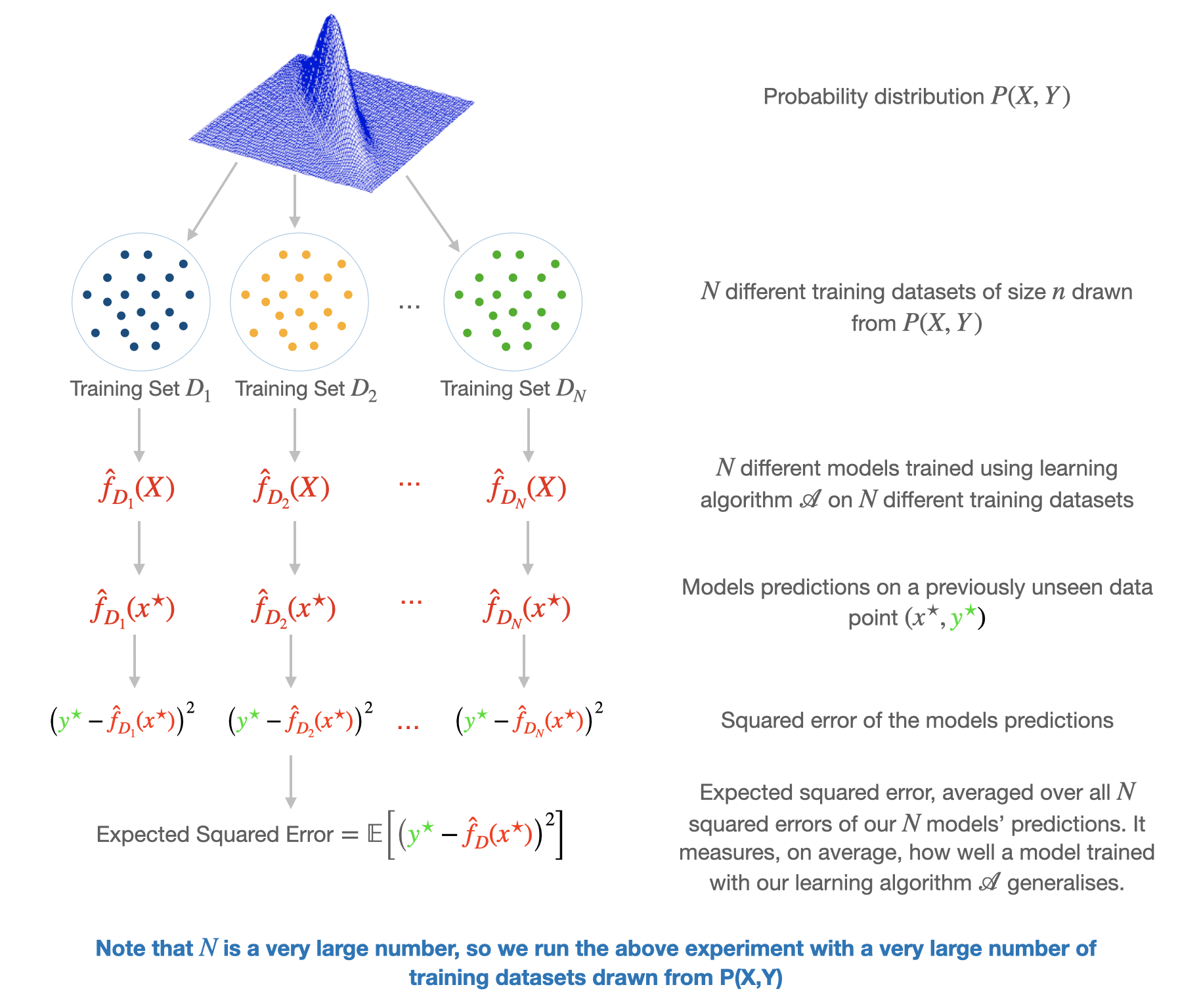
Expectation, Bias, and Variance of model
- Expectation of model $mathbb{E}big[{color{red}hat f_mathcal{D}(x)}big]$
The expectation of the model is the average of the collection of models estimated over many training datasets. - Bias of model $mathbb{E}big[{color{red}hat f_mathcal{D}(x)}big] — color{green}f(x)$
The model bias describes how much the expectation of the model deviates from the true value of the function $color{green}f(x)$ we are trying to estimate. Low bias signifies that our model does a good job of approximating our function, and high bias signifies otherwise. The bias measures the average accuracy of the model. - Variance of model $mathbb{E}Big[Big({color{red}hat f_mathcal{D}(x)} — mathbb{E}big[{color{red}hat f_mathcal{D}(x)}big]Big)^2Big]$
The model variance is the expectation of the squared differences between a particular model and the expectation of the collection of models estimated over many datasets. It captures how much the model fits vary across different datasets, so it measures the average consistency of the model. A learning algorithm with high variance indicates that the models vary a lot across datasets, while low variance indicates that models are quite similar across datasets.
Simulation 1
In practice, the true function we try to estimate is unknown, but for the sake of demonstration, we will assume that the true function is $f(x) = sin(x)$. Individual observations of $y$ will be $y = sin(x) + epsilon$. We assume that $mathbb{E}[epsilon] = 0$ and $text{Var}(epsilon) = sigma^2 = 1.5$. We will sample 50 data sets each with 100 individual observations, and on them we will fit three polynomial functions of varying degrees/complexities (1, 5, 20) to estimate our true function $f(x)$. Degree 1 is the least complex and degree 20 is the most complex.
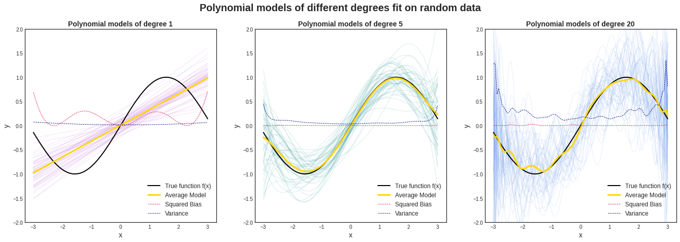
We see from the image above that on average, the degree-1 polynomial model does a bad job of estimating our true function. It has a high bias. The variance is low, which means that the model is consistent across datasets. The degree-20 polynomial model has low bias, which means it does a good job of approximating our true function, but it has a high variance. This means that the model isn’t consistent across datasets. The degree-5 polynomial model has low bias (good estimate of our true function), and a relatively low variance (consistent across datasets).
The code for this simulation can be found here.
A Note on Bias-Variance Tradeoff
Bias-variance tradeoff is the tradeoff in attempting to simultaneously minimise the two sources of error that affect a model’s ability to generalise beyond its training set. Reducing bias generally increases variance and vice versa, and this is a function of a model’s complexity and flexibility. Low variance, high bias models tend to be less complex and less flexible and they mostly underfit the training data, while low bias, high variance models tend to be more complex with a flexible structure that tend to overfit. The optimal model will have both low bias and low variance.
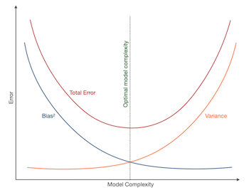
Decomposing Expected Squared Error
As mentioned earlier, it is the expected squared error term in equation (11) that we will decompose into the bias, variance, and irreducible error components. To avoid clutter while decomposing, we will drop the $color{green}star$ sign from $color{green}y^star$ and $color{red}(x^star)$ from $color{red}hat f_mathcal{D}(x^star)$.
$$
tag{12} begin{aligned}
text{Error} & = mathbb{E}Big[Big({color{green}y} — {color{red}hat f_mathcal{D}}Big)^2Big] \
& = mathbb{E}Big[Big({color{green}y} — {color{red}hat f_mathcal{D}}Big)Big({color{green}y} — {color{red}hat f_mathcal{D}}Big)Big] \
& = mathbb{E}Big[ Big({color{green}y}^2 — 2{color{green}y}{color{red}hat f_mathcal{D}} + {color{red}hat f_mathcal{D}}^2 Big)Big] \
& = underbrace{mathbb{E}Big[ {color{green}y}^2 Big]}_{1} + underbrace{mathbb{E}Big[ {color{red}hat f_mathcal{D}}^2 Big]}_{2} — underbrace{2mathbb{E}Big[ {color{green}y}Big]mathbb{E}Big[ {color{red}hat f_mathcal{D}} Big]}_{3}
end{aligned}
$$
Equation (12) has three terms that we will deal with separately. If we consider the third term first, we know that $mathbb{E}big[ {color{red}hat f_mathcal{D}} big]$ is the expectation of our model. If we recall equations (2) and (9) and that $mathbb{E}[{boldsymbolepsilon}] = 0$, we can rewrite $mathbb{E}big[ {color{green}y}big]$ as:
$$
tag{13} begin{aligned}
mathbb{E}Big[ {color{green}y}Big] & = mathbb{E}Big[ {color{green}f(x) + epsilon }Big] \
& = mathbb{E}Big[ {color{green}f(x) }Big] + mathbb{E}Big[ {color{green} epsilon }Big] \
& = {color{green}f(x)}
end{aligned}
$$
For the first and second terms, we use equations (7), (9), and (13) to rewrite them as:
$$
tag{14} begin{aligned}
mathbb{E}Big[ {color{green}y}^2 Big] & = mathbb{E}Big[Big({color{green}y} — {mathbb{E}[{color{green}y}]}Big)^2Big] + {mathbb{E}[{color{green}y}]}^2 \
& = mathbb{E}Big[Big({color{green}f(x) + epsilon } — {color{green}f(x)}Big)^2Big] + {color{green}f(x)}^2 \
& = mathbb{E}Big[{color{green}epsilon}^2 Big] + {color{green}f(x)}^2 \
mathbb{E}Big[ {color{red}hat f_mathcal{D}}^2 Big] & = mathbb{E}Big[Big({color{red}hat f_mathcal{D}} — {mathbb{E}big[{color{red}hat f_mathcal{D}}big]}Big)^2Big] + {mathbb{E}big[{color{red}hat f_mathcal{D}}big]}^2
end{aligned}
$$
Substituting equations (13) and (14) into equation (12), we get:
$$
tag{15} begin{aligned}
text{Error} & = mathbb{E}Big[ {color{green}y}^2 Big] + mathbb{E}Big[ {color{red}hat f_mathcal{D}}^2 Big] — 2mathbb{E}Big[ {color{green}y}Big]mathbb{E}Big[ {color{red}hat f_mathcal{D}} Big]
\
& = mathbb{E}Big[{color{green}epsilon}^2 Big] + {color{green}f(x)}^2 + mathbb{E}Big[Big({color{red}hat f_mathcal{D}} — {mathbb{E}big[{color{red}hat f_mathcal{D}}big]}Big)^2Big] + {mathbb{E}big[{color{red}hat f_mathcal{D}}big]}^2 — 2{color{green}f(x)}mathbb{E}big[ {color{red}hat f_mathcal{D}} big]
end{aligned}
$$
If we rearrange equation (15) and use expansion of squares $(a-b)^2 = a^2 — 2ab + b^2$, we get:
$$
tag{16} begin{aligned}
text{Error} & = underbrace{ {mathbb{E}big[}{color{red}hat f_mathcal{D}} {big]} ^2 — 2{color{green}f(x)}mathbb{E}big[{color{red} hat f_mathcal{D}}big] + {color{green}f(x)}^2 }_{1} + underbrace{mathbb{E}Big[Big({color{red}hat f_mathcal{D}} — {mathbb{E}[{color{red}hat f_mathcal{D}}]}Big)^2Big]}_{2} + underbrace{mathbb{E}Big[{color{green}epsilon}^2 Big]}_{3} \
& = underbrace{Big( {mathbb{E}big[}{color{red}hat f_mathcal{D}} big] — {color{green}f(x)} Big)^2}_{1} + underbrace{mathbb{E}Big[Big({color{red}hat f_mathcal{D}} — {mathbb{E}[{color{red}hat f_mathcal{D}}]}Big)^2Big]}_{2} + underbrace{mathbb{E}Big[{color{green}epsilon}^2 Big]}_{3} \
& = underbrace{Big( {mathbb{E}big[}{color{red}hat f_mathcal{D}} big] — {color{green}f(x)} Big)^2}_{text{Bias}^2 space text{of model}} + underbrace{mathbb{E}Big[Big({color{red}hat f_mathcal{D}} — {mathbb{E}[{color{red}hat f_mathcal{D}}]}Big)^2Big]}_{text{Variance of model}} + underbrace{sigma^2}_{text{Irreducible error}}
end{aligned}
$$
And there is the error decomposed into its three constituent parts. To see a breakdown of how the third term $mathbb{E}Big[{color{green}epsilon}^2 Big]$ became $sigma^2$, you can check the footnote.4
Illustrating Bias-Variance Decomposition using simulated data
In Simulation 1, we estimated our true function $f(x) = sin(x)$ by fitting three polynomial functions of varying complexities. What we really care about though is how our models perform on previously unseen data. In this section, we will demonstrate this and show how the expected squared error decomposes into the sum of variance and squared bias by running the following steps:
- Generate 100 random datasets of 500 observations each from $sin(x) + epsilon$. We assume that the $text{Var}(epsilon) = sigma^2 = 1.5$.
- Split the generated datasets into training and test sets.
- Fit 20 polynomial functions (degrees from 1 to 20) on each of the training sets.
- Predict the value of the test set using the fitted models.
- Calculate the expected prediction error (the mean squared error) on the test set for each model.
- Show the expected prediction error as a sum of the variance and squared bias.
Simulation 2
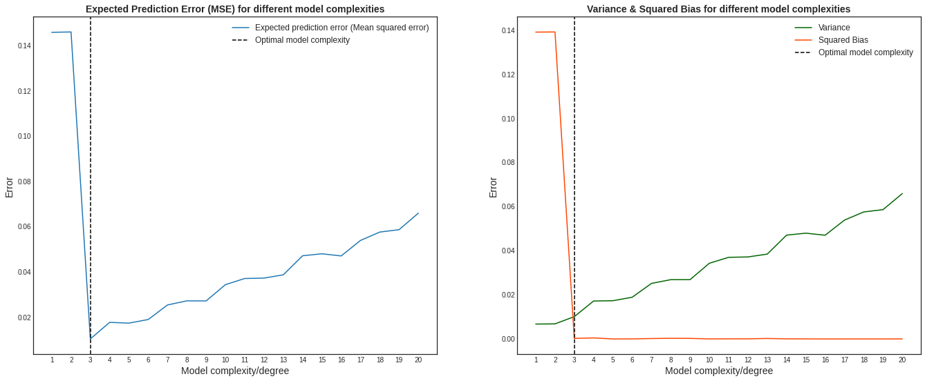
We see from graph on the left in the image above that the error starts quite high, drops off to its minimum at model complexity 3, and then starts climbing rapidly as the complexity increases. If we look at the right graph, we see that it follows the bias-variance tradeoff. The squared-bias of the models drops as the complexity increases, but variance increases. Low bias, high variance models suggest that the models overfit the training data and hence performs poorly on the test data. Our optimal model has low bias and low variance and it is the model with complexity 3 in our simulation.
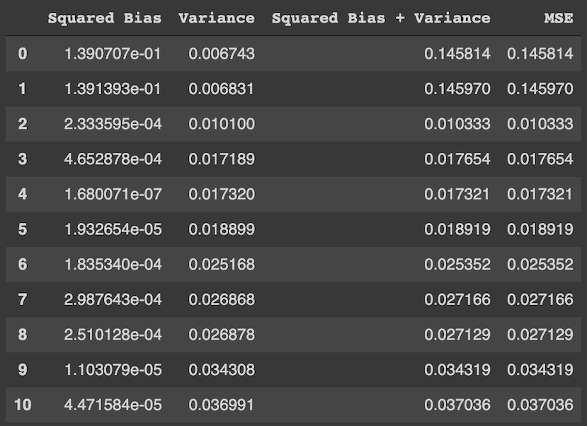
We see from the table above that the mean squared error (MSE) is a sum of the squared bias and the variance, as shown in equation (16). The irreducible part of the decomposition is not added to our sum because we cannot estimate it from data.
The code for this simulation can be found here.
Conclusion
We have shown the decomposition of the generalisation error for regression problems. It is possible to show this decomposition for classification problems. Pedro Domingos’ brilliant paper, A Unified Bias-Variance Decomposition and its Application goes over it in details.
Footnotes
This chapter will begin to dig into some theoretical details of estimating regression functions, in particular how the bias-variance tradeoff helps explain the relationship between model flexibility and the errors a model makes.
Specifically, we will discuss:
- The definitions and relationship between bias, variance, and mean squared error.
- The relationship between model flexibility and training error.
- The relationship between model flexibility and validation error.
Don’t fret if this presentation seems overwhelming. Next chapter we will review some general concepts about regression before moving on to classification.
R Setup and Source
library(tibble)     # data frame printing
library(dplyr)      # data manipulation

library(caret)      # fitting knn
library(rpart)      # fitting trees
library(rpart.plot) # plotting trees
Recall that the Welcome chapter contains directions for installing all necessary packages for following along with the text. The R Markdown source is provided as some code, mostly for creating plots, has been suppressed from the rendered document that you are currently reading.
- R Markdown Source:
bias-variance-tradeoff.Rmd
The Regression Setup
Consider the general regression setup where we are given a random pair ((X, Y) in mathbb{R}^p times mathbb{R}). We would like to “predict” (Y) with some function of (X), say, (f(X)).
To clarify what we mean by “predict,” we specify that we would like (f(X)) to be “close” to (Y). To further clarify what we mean by “close,” we define the squared error loss of estimating (Y) using (f(X)).
[
L(Y, f(X)) triangleq (Y — f(X)) ^ 2
]
Now we can clarify the goal of regression, which is to minimize the above loss, on average. We call this the risk of estimating (Y) using (f(X)).
[
R(Y, f(X)) triangleq mathbb{E}[L(Y, f(X))] = mathbb{E}_{X, Y}[(Y — f(X)) ^ 2]
]
Before attempting to minimize the risk, we first re-write the risk after conditioning on (X).
[
mathbb{E}_{X, Y} left[ (Y — f(X)) ^ 2 right] = mathbb{E}_{X} mathbb{E}_{Y mid X} left[ ( Y — f(X) ) ^ 2 mid X = x right]
]
Minimizing the right-hand side is much easier, as it simply amounts to minimizing the inner expectation with respect to (Y mid X), essentially minimizing the risk pointwise, for each (x).
It turns out, that the risk is minimized by setting (f(x)) to be equal the conditional mean of (Y) given (X),
[
f(x) = mathbb{E}(Y mid X = x)
]
which we call the regression function.63
Note that the choice of squared error loss is somewhat arbitrary. Suppose instead we chose absolute error loss.
[
L(Y, f(X)) triangleq | Y — f(X) |
]
The risk would then be minimized setting (f(x)) equal to the conditional median.
[
f(x) = text{median}(Y mid X = x)
]
Despite this possibility, our preference will still be for squared error loss. The reasons for this are numerous, including: historical, ease of optimization, and protecting against large deviations.
Now, given data (mathcal{D} = (x_i, y_i) in mathbb{R}^p times mathbb{R}), our goal becomes finding some (hat{f}) that is a good estimate of the regression function (f). We’ll see that this amounts to minimizing what we call the reducible error.
Reducible and Irreducible Error
Suppose that we obtain some (hat{f}), how well does it estimate (f)? We define the expected prediction error of predicting (Y) using (hat{f}(X)). A good (hat{f}) will have a low expected prediction error.
[
text{EPE}left(Y, hat{f}(X)right) triangleq mathbb{E}_{X, Y, mathcal{D}} left[ left( Y — hat{f}(X) right)^2 right]
]
This expectation is over (X), (Y), and also (mathcal{D}). The estimate (hat{f}) is actually random depending on the data, (mathcal{D}), used to estimate (hat{f}). We could actually write (hat{f}(X, mathcal{D})) to make this dependence explicit, but our notation will become cumbersome enough as it is.
Like before, we’ll condition on (X). This results in the expected prediction error of predicting (Y) using (hat{f}(X)) when (X = x).
[
text{EPE}left(Y, hat{f}(x)right) =
mathbb{E}_{Y mid X, mathcal{D}} left[ left(Y — hat{f}(X) right)^2 mid X = x right] =
underbrace{mathbb{E}_{mathcal{D}} left[ left(f(x) — hat{f}(x) right)^2 right]}_textrm{reducible error} +
underbrace{mathbb{V}_{Y mid X} left[ Y mid X = x right]}_textrm{irreducible error}
]
A number of things to note here:
- The expected prediction error is for a random (Y) given a fixed (x) and a random (hat{f}). As such, the expectation is over (Y mid X) and (mathcal{D}). Our estimated function (hat{f}) is random depending on the data, (mathcal{D}), which is used to perform the estimation.
- The expected prediction error of predicting (Y) using (hat{f}(X)) when (X = x) has been decomposed into two errors:
- The reducible error, which is the expected squared error loss of estimation (f(x)) using (hat{f}(x)) at a fixed point (x). The only thing that is random here is (mathcal{D}), the data used to obtain (hat{f}). (Both (f) and (x) are fixed.) We’ll often call this reducible error the mean squared error of estimating (f(x)) using (hat{f}) at a fixed point (x). [
text{MSE}left(f(x), hat{f}(x)right) triangleq
mathbb{E}_{mathcal{D}} left[ left(f(x) — hat{f}(x) right)^2 right]] - The irreducible error. This is simply the variance of (Y) given that (X = x), essentially noise that we do not want to learn. This is also called the Bayes error.
- The reducible error, which is the expected squared error loss of estimation (f(x)) using (hat{f}(x)) at a fixed point (x). The only thing that is random here is (mathcal{D}), the data used to obtain (hat{f}). (Both (f) and (x) are fixed.) We’ll often call this reducible error the mean squared error of estimating (f(x)) using (hat{f}) at a fixed point (x). [
As the name suggests, the reducible error is the error that we have some control over. But how do we control this error?
Bias-Variance Decomposition
After decomposing the expected prediction error into reducible and irreducible error, we can further decompose the reducible error.
Recall the definition of the bias of an estimator.
[
text{bias}(hat{theta}) triangleq mathbb{E}left[hat{theta}right] — theta
]
Also recall the definition of the variance of an estimator.
[
mathbb{V}(hat{theta}) = text{var}(hat{theta}) triangleq mathbb{E}left [ ( hat{theta} -mathbb{E}left[hat{theta}right] )^2 right]
]
Using this, we further decompose the reducible error (mean squared error) into bias squared and variance.
[
text{MSE}left(f(x), hat{f}(x)right) =
mathbb{E}_{mathcal{D}} left[ left(f(x) — hat{f}(x) right)^2 right] =
underbrace{left(f(x) — mathbb{E} left[ hat{f}(x) right] right)^2}_{text{bias}^2 left(hat{f}(x) right)} +
underbrace{mathbb{E} left[ left( hat{f}(x) — mathbb{E} left[ hat{f}(x) right] right)^2 right]}_{text{var} left(hat{f}(x) right)}
]
This is actually a common fact in estimation theory, but we have stated it here specifically for estimation of some regression function (f) using (hat{f}) at some point (x).
[
text{MSE}left(f(x), hat{f}(x)right) = text{bias}^2 left(hat{f}(x) right) + text{var} left(hat{f}(x) right)
]
In a perfect world, we would be able to find some (hat{f}) which is unbiased, that is (text{bias}left(hat{f}(x) right) = 0), which also has low variance. In practice, this isn’t always possible.
It turns out, there is a bias-variance tradeoff. That is, often, the more bias in our estimation, the lesser the variance. Similarly, less variance is often accompanied by more bias. Flexible models tend to be unbiased, but highly variable. Simple models are often extremely biased, but have low variance.
In the context of regression, models are biased when:
- Parametric: The form of the model does not incorporate all the necessary variables, or the form of the relationship is too simple. For example, a parametric model assumes a linear relationship, but the true relationship is quadratic.
- Non-parametric: The model provides too much smoothing.
In the context of regression, models are variable when:
- Parametric: The form of the model incorporates too many variables, or the form of the relationship is too flexible. For example, a parametric model assumes a cubic relationship, but the true relationship is linear.
- Non-parametric: The model does not provide enough smoothing. It is very, “wiggly.”
So for us, to select a model that appropriately balances the tradeoff between bias and variance, and thus minimizes the reducible error, we need to select a model of the appropriate flexibility for the data.
Recall that when fitting models, we’ve seen that train RMSE decreases as model flexibility is increasing. (Technically it is non-increasing.) For validation RMSE, we expect to see a U-shaped curve. Importantly, validation RMSE decreases, until a certain flexibility, then begins to increase.
Now we can understand why this is happening. The expected test RMSE is essentially the expected prediction error, which we now known decomposes into (squared) bias, variance, and the irreducible Bayes error. The following plots show three examples of this.
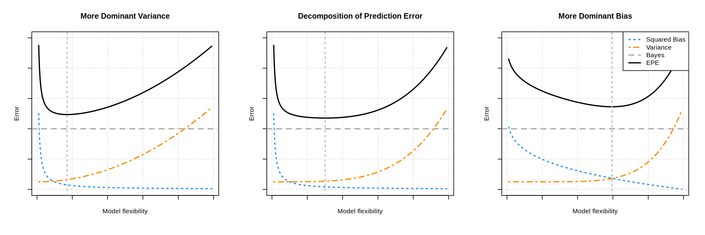
The three plots show three examples of the bias-variance tradeoff. In the left panel, the variance influences the expected prediction error more than the bias. In the right panel, the opposite is true. The middle panel is somewhat neutral. In all cases, the difference between the Bayes error (the horizontal dashed grey line) and the expected prediction error (the solid black curve) is exactly the mean squared error, which is the sum of the squared bias (blue curve) and variance (orange curve). The vertical line indicates the flexibility that minimizes the prediction error.
To summarize, if we assume that irreducible error can be written as
[
mathbb{V}[Y mid X = x] = sigma ^ 2
]
then we can write the full decomposition of the expected prediction error of predicting (Y) using (hat{f}) when (X = x) as
[
text{EPE}left(Y, hat{f}(x)right) =
underbrace{text{bias}^2left(hat{f}(x)right) + text{var}left(hat{f}(x)right)}_textrm{reducible error} + sigma^2.
]
As model flexibility increases, bias decreases, while variance increases. By understanding the tradeoff between bias and variance, we can manipulate model flexibility to find a model that will predict well on unseen observations.
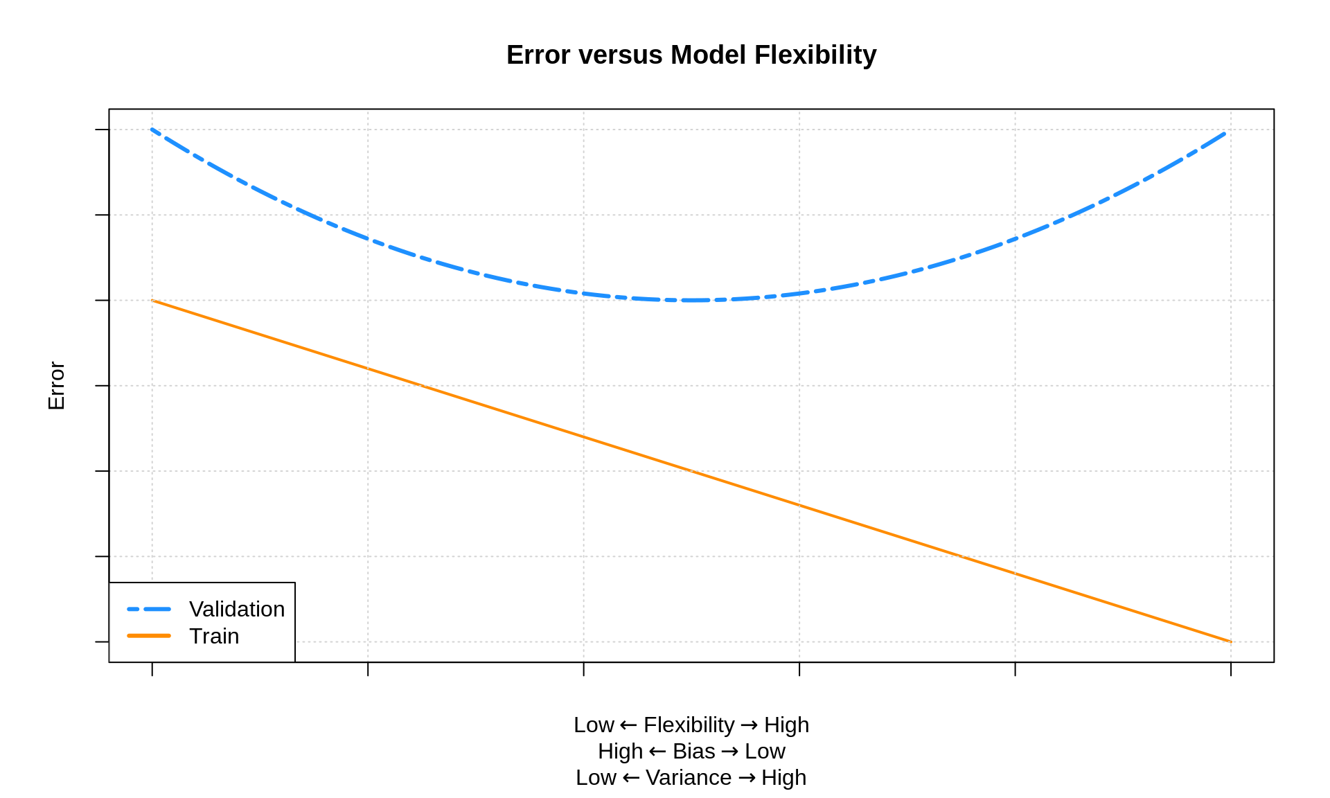
Tying this all together, the above image shows how we “expect” training and validation error to behavior in relation to model flexibility.64 In practice, we won’t always see such a nice “curve” in the validation error, but we expect to see the general trends.
Using Simulation to Estimate Bias and Variance
We will illustrate these decompositions, most importantly the bias-variance tradeoff, through simulation. Suppose we would like to train a model to learn the true regression function function (f(x) = x^2).
f = function(x) {
  x ^ 2
}
More specifically, we’d like to predict an observation, (Y), given that (X = x) by using (hat{f}(x)) where
[
mathbb{E}[Y mid X = x] = f(x) = x^2
]
and
[
mathbb{V}[Y mid X = x] = sigma ^ 2.
]
Alternatively, we could write this as
[
Y = f(X) + epsilon
]
where (mathbb{E}[epsilon] = 0) and (mathbb{V}[epsilon] = sigma ^ 2). In this formulation, we call (f(X)) the signal and (epsilon) the noise.
To carry out a concrete simulation example, we need to fully specify the data generating process. We do so with the following R code.
gen_sim_data = function(f, sample_size = 100) {
  x = runif(n = sample_size, min = 0, max = 1)
  y = rnorm(n = sample_size, mean = f(x), sd = 0.3)
  tibble(x, y)
}
Also note that if you prefer to think of this situation using the (Y = f(X) + epsilon) formulation, the following code represents the same data generating process.
gen_sim_data = function(f, sample_size = 100) {
  x = runif(n = sample_size, min = 0, max = 1)
  eps = rnorm(n = sample_size, mean = 0, sd = 0.75)
  y = f(x) + eps
  tibble(x, y)
}
To completely specify the data generating process, we have made more model assumptions than simply (mathbb{E}[Y mid X = x] = x^2) and (mathbb{V}[Y mid X = x] = sigma ^ 2). In particular,
- The (x_i) in (mathcal{D}) are sampled from a uniform distribution over ([0, 1]).
- The (x_i) and (epsilon) are independent.
- The (y_i) in (mathcal{D}) are sampled from the conditional normal distribution.
[
Y mid X sim N(f(x), sigma^2)
]
Using this setup, we will generate datasets, (mathcal{D}), with a sample size (n = 100) and fit four models.
[
begin{aligned}
texttt{predict(fit0, x)} &= hat{f}_0(x) = hat{beta}_0\
texttt{predict(fit1, x)} &= hat{f}_1(x) = hat{beta}_0 + hat{beta}_1 x \
texttt{predict(fit2, x)} &= hat{f}_2(x) = hat{beta}_0 + hat{beta}_1 x + hat{beta}_2 x^2 \
texttt{predict(fit9, x)} &= hat{f}_9(x) = hat{beta}_0 + hat{beta}_1 x + hat{beta}_2 x^2 + ldots + hat{beta}_9 x^9
end{aligned}
]
To get a sense of the data and these four models, we generate one simulated dataset, and fit the four models.
set.seed(1)
sim_data = gen_sim_data(f)fit_0 = lm(y ~ 1, data = sim_data)
fit_1 = lm(y ~ poly(x, degree = 1), data = sim_data)
fit_2 = lm(y ~ poly(x, degree = 2), data = sim_data)
fit_9 = lm(y ~ poly(x, degree = 9), data = sim_data)Note that technically we’re being lazy and using orthogonal polynomials, but the fitted values are the same, so this makes no difference for our purposes.
Plotting these four trained models, we see that the zero predictor model does very poorly. The first degree model is reasonable, but we can see that the second degree model fits much better. The ninth degree model seem rather wild.
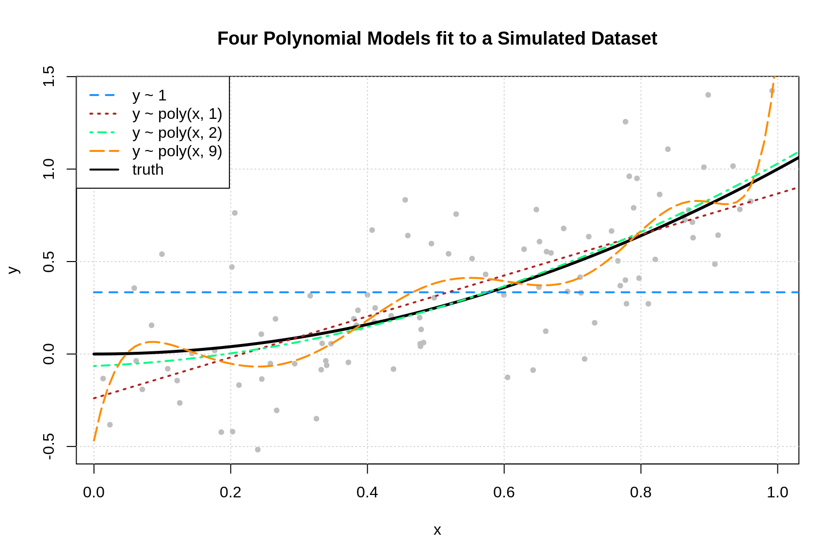
The following three plots were created using three additional simulated datasets. The zero predictor and ninth degree polynomial were fit to each.
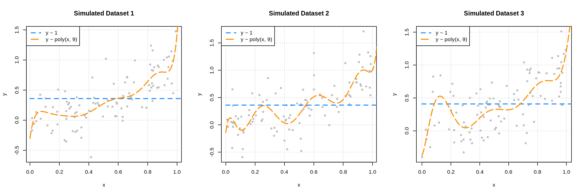
This plot should make clear the difference between the bias and variance of these two models. The zero predictor model is clearly wrong, that is, biased, but nearly the same for each of the datasets, since it has very low variance.
While the ninth degree model doesn’t appear to be correct for any of these three simulations, we’ll see that on average it is, and thus is performing unbiased estimation. These plots do however clearly illustrate that the ninth degree polynomial is extremely variable. Each dataset results in a very different fitted model. Correct on average isn’t the only goal we’re after, since in practice, we’ll only have a single dataset. This is why we’d also like our models to exhibit low variance.
We could have also fit (k)-nearest neighbors models to these three datasets.
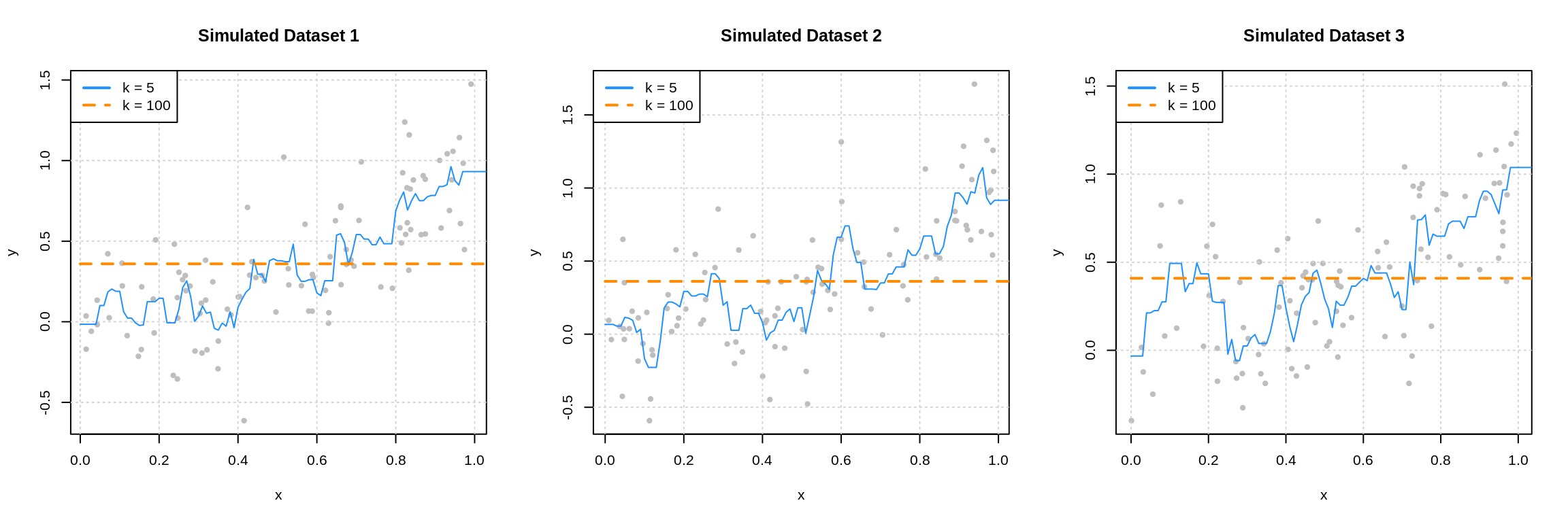
Here we see that when (k = 100) we have a biased model with very low variance.65 When (k = 5), we again have a highly variable model.
These two sets of plots reinforce our intuition about the bias-variance tradeoff. Flexible models (ninth degree polynomial and (k) = 5) are highly variable, and often unbiased. Simple models (zero predictor linear model and (k = 100)) are very biased, but have extremely low variance.
We will now complete a simulation study to understand the relationship between the bias, variance, and mean squared error for the estimates of (f(x)) given by these four models at the point (x = 0.90). We use simulation to complete this task, as performing the analytical calculations would prove to be rather tedious and difficult.
set.seed(1)
n_sims = 250
n_models = 4
x = data.frame(x = 0.90) # fixed point at which we make predictions
predictions = matrix(0, nrow = n_sims, ncol = n_models)for (sim in 1:n_sims) {
# simulate new, random, training data
# this is the only random portion of the bias, var, and mse calculations
# this allows us to calculate the expectation over D
sim_data = gen_sim_data(f)
# fit models
fit_0 = lm(y ~ 1,                   data = sim_data)
fit_1 = lm(y ~ poly(x, degree = 1), data = sim_data)
fit_2 = lm(y ~ poly(x, degree = 2), data = sim_data)
fit_9 = lm(y ~ poly(x, degree = 9), data = sim_data)
# get predictions
predictions[sim, 1] = predict(fit_0, x)
predictions[sim, 2] = predict(fit_1, x)
predictions[sim, 3] = predict(fit_2, x)
predictions[sim, 4] = predict(fit_9, x)
}Note that this is one of many ways we could have accomplished this task using R. For example we could have used a combination of replicate() and *apply() functions. Alternatively, we could have used a tidyverse approach, which likely would have used some combination of dplyr, tidyr, and purrr.
Our approach, which would be considered a base R approach, was chosen to make it as clear as possible what is being done. The tidyverse approach is rapidly gaining popularity in the R community, but might make it more difficult to see what is happening here, unless you are already familiar with that approach.
Also of note, while it may seem like the output stored in predictions would meet the definition of tidy data given by Hadley Wickham since each row represents a simulation, it actually falls slightly short. For our data to be tidy, a row should store the simulation number, the model, and the resulting prediction. We’ve actually already aggregated one level above this. Our observational unit is a simulation (with four predictions), but for tidy data, it should be a single prediction.
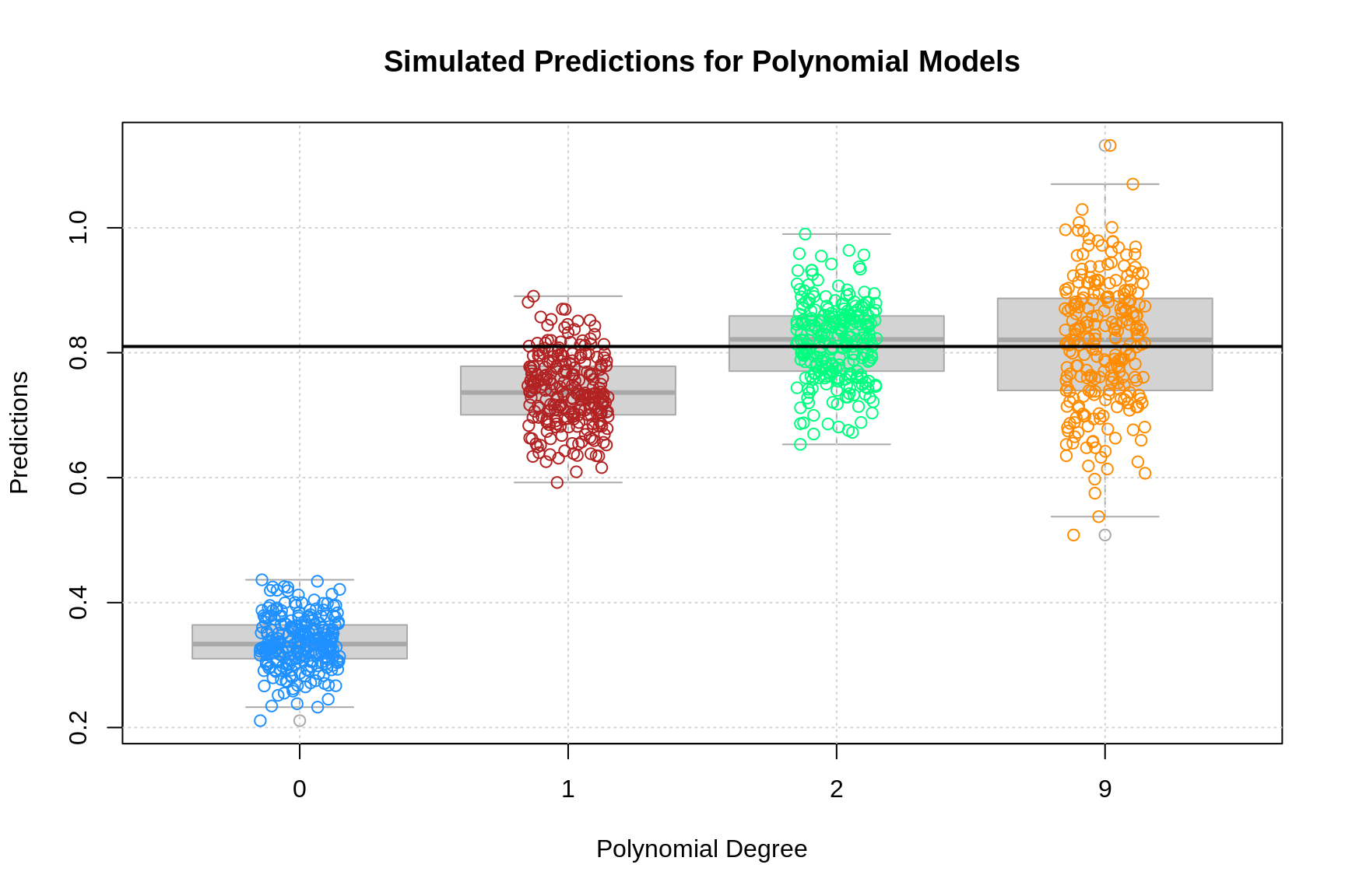
The above plot shows the predictions for each of the 250 simulations of each of the four models of different polynomial degrees. The truth, (f(x = 0.90) = (0.9)^2 = 0.81), is given by the solid black horizontal line.
Two things are immediately clear:
- As flexibility increases, bias decreases. The mean of a model’s predictions is closer to the truth.
- As flexibility increases, variance increases. The variance about the mean of a model’s predictions increases.
The goal of this simulation study is to show that the following holds true for each of the four models.
[
text{MSE}left(f(0.90), hat{f}_k(0.90)right) =
underbrace{left(mathbb{E} left[ hat{f}_k(0.90) right] — f(0.90) right)^2}_{text{bias}^2 left(hat{f}_k(0.90) right)} +
underbrace{mathbb{E} left[ left( hat{f}_k(0.90) — mathbb{E} left[ hat{f}_k(0.90) right] right)^2 right]}_{text{var} left(hat{f}_k(0.90) right)}
]
We’ll use the empirical results of our simulations to estimate these quantities. (Yes, we’re using estimation to justify facts about estimation.) Note that we’ve actually used a rather small number of simulations. In practice we should use more, but for the sake of computation time, we’ve performed just enough simulations to obtain the desired results. (Since we’re estimating estimation, the bigger the sample size, the better.)
To estimate the mean squared error of our predictions, we’ll use
[
widehat{text{MSE}}left(f(0.90), hat{f}_k(0.90)right) = frac{1}{n_{texttt{sims}}}sum_{i = 1}^{n_{texttt{sims}}} left(f(0.90) — hat{f}_k^{[i]}(0.90) right)^2
]
where (hat{f}_k^{[i]}(0.90)) is the estimate of (f(0.90)) using the (i)-th from the polynomial degree (k) model.
We also write an accompanying R function.
get_mse = function(truth, estimate) {
  mean((estimate - truth) ^ 2)
}
Similarly, for the bias of our predictions we use,
[
widehat{text{bias}} left(hat{f}(0.90) right) = frac{1}{n_{texttt{sims}}}sum_{i = 1}^{n_{texttt{sims}}} left(hat{f}_k^{[i]}(0.90) right) — f(0.90)
]
And again, we write an accompanying R function.
get_bias = function(estimate, truth) {
  mean(estimate) - truth
}
Lastly, for the variance of our predictions we have
[
widehat{text{var}} left(hat{f}(0.90) right) = frac{1}{n_{texttt{sims}}}sum_{i = 1}^{n_{texttt{sims}}} left(hat{f}_k^{[i]}(0.90) — frac{1}{n_{texttt{sims}}}sum_{i = 1}^{n_{texttt{sims}}}hat{f}_k^{[i]}(0.90) right)^2
]
While there is already R function for variance, the following is more appropriate in this situation.
get_var = function(estimate) {
  mean((estimate - mean(estimate)) ^ 2)
}
To quickly obtain these results for each of the four models, we utilize the apply() function.
bias = apply(predictions, 2, get_bias, truth = f(x = 0.90))
variance = apply(predictions, 2, get_var)
mse = apply(predictions, 2, get_mse, truth = f(x = 0.90))
We summarize these results in the following table.
| Degree | Mean Squared Error | Bias Squared | Variance |
|---|---|---|---|
| 0 | 0.22643 | 0.22476 | 0.00167 |
| 1 | 0.00829 | 0.00508 | 0.00322 |
| 2 | 0.00387 | 0.00005 | 0.00381 |
| 9 | 0.01019 | 0.00002 | 0.01017 |
A number of things to notice here:
- We use squared bias in this table. Since bias can be positive or negative, squared bias is more useful for observing the trend as flexibility increases.
- The squared bias trend which we see here is decreasing as flexibility increases, which we expect to see in general.
- The exact opposite is true of variance. As model flexibility increases, variance increases.
- The mean squared error, which is a function of the bias and variance, decreases, then increases. This is a result of the bias-variance tradeoff. We can decrease bias, by increasing variance. Or, we can decrease variance by increasing bias. By striking the correct balance, we can find a good mean squared error!
We can check for these trends with the diff() function in R.
## [1] TRUE## [1] TRUE## 1 2 9
## TRUE TRUE FALSEThe models with polynomial degrees 2 and 9 are both essentially unbiased. We see some bias here as a result of using simulation. If we increased the number of simulations, we would see both biases go down. Since they are both unbiased, the model with degree 2 outperforms the model with degree 9 due to its smaller variance.
Models with degree 0 and 1 are biased because they assume the wrong form of the regression function. While the degree 9 model does this as well, it does include all the necessary polynomial degrees.
[
hat{f}_9(x) = hat{beta}_0 + hat{beta}_1 x + hat{beta}_2 x^2 + ldots + hat{beta}_9 x^9
]
Then, since least squares estimation is unbiased, importantly,
[
mathbb{E}left[hat{beta}_dright] = beta_d = 0
]
for (d = 3, 4, ldots 9), we have
[
mathbb{E}left[hat{f}_9(x)right] = beta_0 + beta_1 x + beta_2 x^2
]
Now we can finally verify the bias-variance decomposition.
bias ^ 2 + variance == mse## 0 1 2 9
## FALSE FALSE FALSE FALSEBut wait, this says it isn’t true, except for the degree 9 model? It turns out, this is simply a computational issue. If we allow for some very small error tolerance, we see that the bias-variance decomposition is indeed true for predictions from these for models.
all.equal(bias ^ 2 + variance, mse)## [1] TRUESee ?all.equal() for details.
So far, we’ve focused our efforts on looking at the mean squared error of estimating (f(0.90)) using (hat{f}(0.90)). We could also look at the expected prediction error of using (hat{f}(X)) when (X = 0.90) to estimate (Y).
[
text{EPE}left(Y, hat{f}_k(0.90)right) =
mathbb{E}_{Y mid X, mathcal{D}} left[ left(Y — hat{f}_k(X) right)^2 mid X = 0.90 right]
]
We can estimate this quantity for each of the four models using the simulation study we already performed.
get_epe = function(realized, estimate) {
  mean((realized - estimate) ^ 2)
}
y = rnorm(n = nrow(predictions), mean = f(x = 0.9), sd = 0.3)
epe = apply(predictions, 2, get_epe, realized = y)
epe## 0 1 2 9
## 0.3180470 0.1104055 0.1095955 0.1205570What about the unconditional expected prediction error. That is, for any (X), not just (0.90). Specifically, the expected prediction error of estimating (Y) using (hat{f}(X)). The following (new) simulation study provides an estimate of
[
text{EPE}left(Y, hat{f}_k(X)right) = mathbb{E}_{X, Y, mathcal{D}} left[ left( Y — hat{f}_k(X) right)^2 right]
]
for the quadratic model, that is (k = 2) as we have defined (k).
set.seed(42)
n_sims = 2500
X = runif(n = n_sims, min = 0, max = 1)
Y = rnorm(n = n_sims, mean = f(X), sd = 0.3)

f_hat_X = rep(0, length(X))

for (i in seq_along(X)) {
  sim_data = gen_sim_data(f)
  fit_2 = lm(y ~ poly(x, degree = 2), data = sim_data)
  f_hat_X[i] = predict(fit_2, newdata = data.frame(x = X[i]))
}
## [1] 0.09# via simulation
mean((Y - f_hat_X) ^ 2)## [1] 0.09566445Note that in practice, we should use many more simulations in this study.
Estimating Expected Prediction Error
While previously, we only decomposed the expected prediction error conditionally, a similar argument holds unconditionally.
Assuming
[
mathbb{V}[Y mid X = x] = sigma ^ 2.
]
we have
[
text{EPE}left(Y, hat{f}(X)right) =
mathbb{E}_{X, Y, mathcal{D}} left[ (Y — hat{f}(X))^2 right] =
underbrace{mathbb{E}_{X} left[text{bias}^2left(hat{f}(X)right)right] + mathbb{E}_{X} left[text{var}left(hat{f}(X)right)right]}_textrm{reducible error} + sigma^2
]
Lastly, we note that if
[
mathcal{D} = mathcal{D}_{texttt{trn}} cup mathcal{D}_{texttt{tst}} = (x_i, y_i) in mathbb{R}^p times mathbb{R}, i = 1, 2, ldots n
]
where
[
mathcal{D}_{texttt{trn}} = (x_i, y_i) in mathbb{R}^p times mathbb{R}, i in texttt{trn}
]
and
[
mathcal{D}_{texttt{tst}} = (x_i, y_i) in mathbb{R}^p times mathbb{R}, i in texttt{tst}
]
Then, if we have a model fit to the training data (mathcal{D}_{texttt{trn}}), we can use the test mean squared error
[
sum_{i in texttt{tst}}left(y_i — hat{f}(x_i)right) ^ 2
]
as an estimate of
[
mathbb{E}_{X, Y, mathcal{D}} left[ (Y — hat{f}(X))^2 right]
]
the expected prediction error.66
How good is this estimate? Well, if (mathcal{D}) is a random sample from ((X, Y)), and the (texttt{tst}) data are randomly sampled observations randomly sampled from (i = 1, 2, ldots, n), then it is a reasonable estimate. However, it is rather variable due to the randomness of selecting the observations for the test set, if the test set is small.
Model Flexibility
Let’s return to the dataset we saw in the linear regression chapter with a single feature (x).
# define regression function
cubic_mean = function(x) {
  1 - 2 * x - 3 * x ^ 2 + 5 * x ^ 3
}
Recall that this data was generated with a cubic mean function.
# define full data generating process
gen_slr_data = function(sample_size = 100, mu) {
  x = runif(n = sample_size, min = -1, max = 1)
  y = mu(x) + rnorm(n = sample_size)
  tibble(x, y)
}
After defining the data generating process, we generate and split the data.
# simulate entire dataset
set.seed(3)
sim_slr_data = gen_slr_data(sample_size = 100, mu = cubic_mean)

# test-train split
slr_trn_idx = sample(nrow(sim_slr_data), size = 0.8 * nrow(sim_slr_data))
slr_trn = sim_slr_data[slr_trn_idx, ]
slr_tst = sim_slr_data[-slr_trn_idx, ]

# estimation-validation split
slr_est_idx = sample(nrow(slr_trn), size = 0.8 * nrow(slr_trn))
slr_est = slr_trn[slr_est_idx, ]
slr_val = slr_trn[-slr_est_idx, ]

# check data
head(slr_trn, n = 10)
## # A tibble: 10 x 2
## x y
## <dbl> <dbl>
## 1 0.573 -1.18
## 2 0.807 0.576
## 3 0.272 -0.973
## 4 -0.813 -1.78
## 5 -0.161 0.833
## 6 0.736 1.07
## 7 -0.242 2.97
## 8 0.520 -1.64
## 9 -0.664 0.269
## 10 -0.777 -2.02For validating models, we will use RMSE.
# helper function for calculating RMSE
calc_rmse = function(actual, predicted) {
  sqrt(mean((actual - predicted) ^ 2))
}
Let’s check how linear, k-nearest neighbors, and decision tree models fit to this data make errors, while paying attention to their flexibility.
This picture is an idealized version of what we expect to see, but we’ll illustrate the sorts of validate “curves” that we might see in practice.
Note that in the following three sub-sections, a significant portion of the code is suppressed for visual clarity. See the source document for full details.
Linear Models
First up, linear models. We will fit polynomial models with degree from one to nine, and then validate.
# fit polynomial models
poly_mod_est_list = list(
  poly_mod_1_est = lm(y ~ poly(x, degree = 1), data = slr_est),
  poly_mod_2_est = lm(y ~ poly(x, degree = 2), data = slr_est),
  poly_mod_3_est = lm(y ~ poly(x, degree = 3), data = slr_est),
  poly_mod_4_est = lm(y ~ poly(x, degree = 4), data = slr_est),
  poly_mod_5_est = lm(y ~ poly(x, degree = 5), data = slr_est),
  poly_mod_6_est = lm(y ~ poly(x, degree = 6), data = slr_est),
  poly_mod_7_est = lm(y ~ poly(x, degree = 7), data = slr_est),
  poly_mod_8_est = lm(y ~ poly(x, degree = 8), data = slr_est),
  poly_mod_9_est = lm(y ~ poly(x, degree = 9), data = slr_est)
)
The plot below visualizes the results.
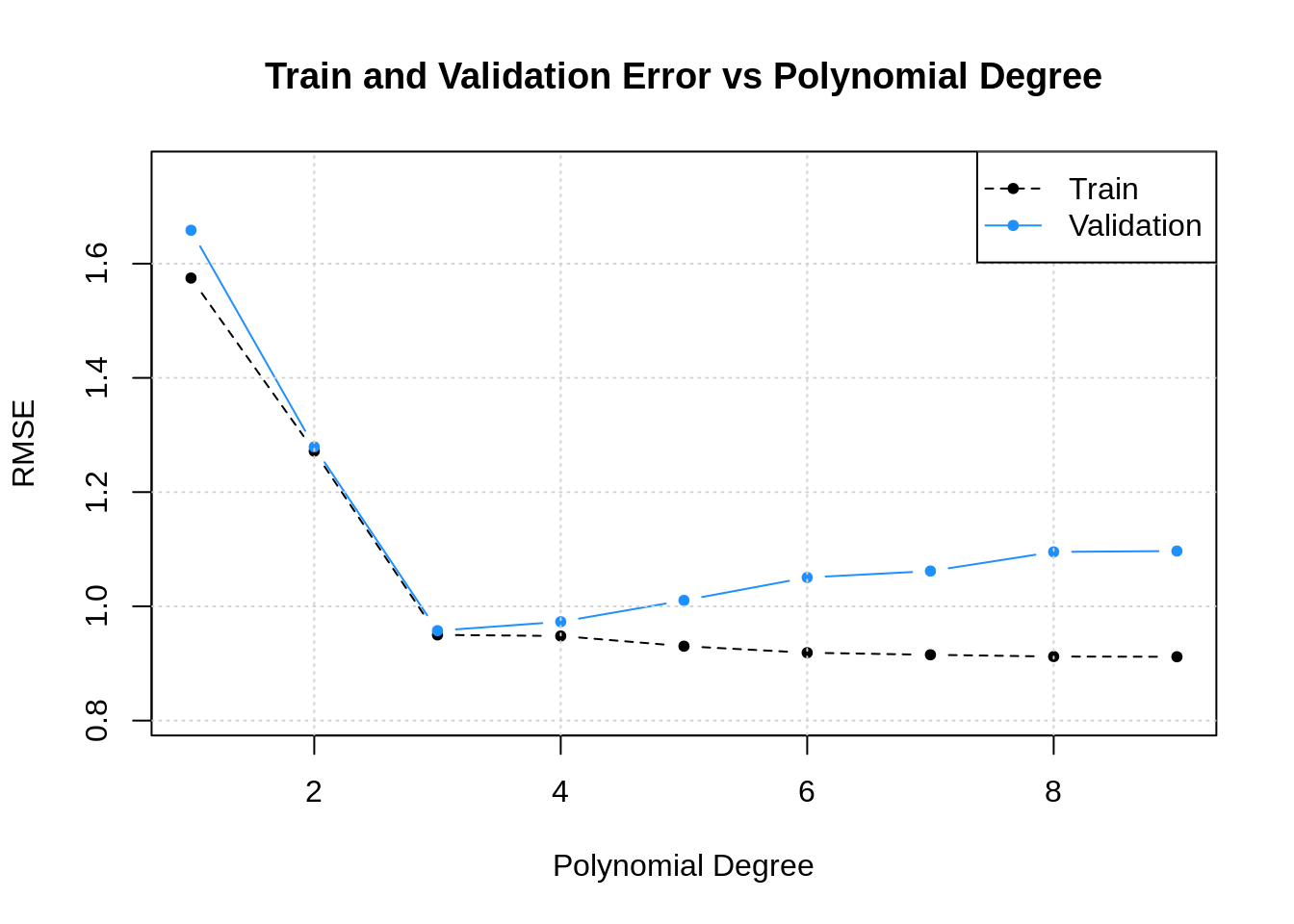
What do we see here? As the polynomial degree increases:
- The training error decreases.
- The validation error decreases, then increases.
This more of less matches the idealized version above, but the validation “curve” is much more jagged. This is something that we can expect in practice.
We have previously noted that training error isn’t particularly useful for validating models. That is still true. However, it can be useful for checking that everything is working as planned. In this case, since we known that training error decreases as model flexibility increases, we can verify our intuition that a higher degree polynomial is indeed more flexible.67
k-Nearest Neighbors
Next up, k-nearest neighbors. We will consider values for (k) that are odd and between (1) and (45) inclusive.
# helper function for fitting knn models
fit_knn_mod = function(neighbors) {
  knnreg(y ~ x, data = slr_est, k = neighbors)
}
# define values of tuning parameter k to evaluate
k_to_try = seq(from = 1, to = 45, by = 2)
# fit knn models
knn_mod_est_list = lapply(k_to_try, fit_knn_mod)The plot below visualizes the results.
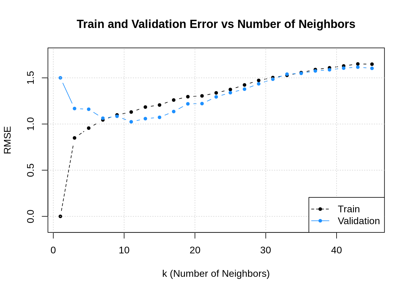
Here we see the “opposite” of the usual plot. Why? Because with k-nearest neighbors, a small value of (k) generates a flexible model compared to larger values of (k). So visually, this plot is flipped. That is we see that as (k) increases:
- The training error increases.
- The validation error decreases, then increases.
Important to note here: the pattern above only holds “in general,” that is, there can be minor deviations in the validation pattern along the way. This is due to the random nature of selection the data for the validate set.
Decision Trees
Lastly, we evaluate some decision tree models. We choose some arbitrary values of cp to evaluate, while holding minsplit constant at 5. There are arbitrary choices that produce a plot that is useful for discussion.
# helper function for fitting decision tree models
tree_knn_mod = function(flex) {
  rpart(y ~ x, data = slr_est, cp = flex, minsplit = 5)
}
# define values of tuning parameter cp to evaluate
cp_to_try = c(0.5, 0.3, 0.1, 0.05, 0.01, 0.001, 0.0001)
# fit decision tree models
tree_mod_est_list = lapply(cp_to_try, tree_knn_mod)The plot below visualizes the results.
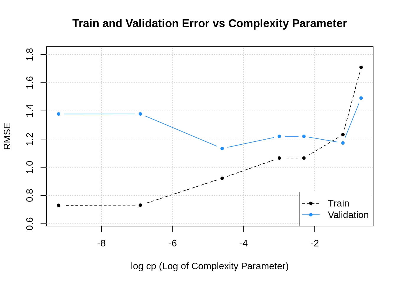
Based on this plot, how is cp related to model flexibility?68