Mean squared error формула

From Wikipedia, the free encyclopedia

In statistics, the mean squared error (MSE)^[1] or mean squared deviation (MSD) of an estimator (of a procedure for estimating an unobserved quantity) measures the average of the squares of the errors—that is, the average squared difference between the estimated values and the actual value. MSE is a risk function, corresponding to the expected value of the squared error loss.^[2] The fact that MSE is almost always strictly positive (and not zero) is because of randomness or because the estimator does not account for information that could produce a more accurate estimate.^[3] In machine learning, specifically empirical risk minimization, MSE may refer to the empirical risk (the average loss on an observed data set), as an estimate of the true MSE (the true risk: the average loss on the actual population distribution).

The MSE is a measure of the quality of an estimator. As it is derived from the square of Euclidean distance, it is always a positive value that decreases as the error approaches zero.

The MSE is the second moment (about the origin) of the error, and thus incorporates both the variance of the estimator (how widely spread the estimates are from one data sample to another) and its bias (how far off the average estimated value is from the true value).^{[citation needed]} For an unbiased estimator, the MSE is the variance of the estimator. Like the variance, MSE has the same units of measurement as the square of the quantity being estimated. In an analogy to standard deviation, taking the square root of MSE yields the root-mean-square error or root-mean-square deviation (RMSE or RMSD), which has the same units as the quantity being estimated; for an unbiased estimator, the RMSE is the square root of the variance, known as the standard error.

Definition and basic properties[edit]

The MSE either assesses the quality of a predictor (i.e., a function mapping arbitrary inputs to a sample of values of some random variable), or of an estimator (i.e., a mathematical function mapping a sample of data to an estimate of a parameter of the population from which the data is sampled). The definition of an MSE differs according to whether one is describing a predictor or an estimator.

Predictor[edit]

If a vector of predictions is generated from a sample of data points on all variables, and is the vector of observed values of the variable being predicted, with being the predicted values (e.g. as from a least-squares fit), then the within-sample MSE of the predictor is computed as

In other words, the MSE is the mean of the squares of the errors . This is an easily computable quantity for a particular sample (and hence is sample-dependent).

In matrix notation,

where is and is the column vector.

The MSE can also be computed on q data points that were not used in estimating the model, either because they were held back for this purpose, or because these data have been newly obtained. Within this process, known as statistical learning, the MSE is often called the test MSE,^[4] and is computed as

Estimator[edit]

The MSE of an estimator with respect to an unknown parameter is defined as^[1]

This definition depends on the unknown parameter, but the MSE is a priori a property of an estimator. The MSE could be a function of unknown parameters, in which case any estimator of the MSE based on estimates of these parameters would be a function of the data (and thus a random variable). If the estimator is derived as a sample statistic and is used to estimate some population parameter, then the expectation is with respect to the sampling distribution of the sample statistic.

The MSE can be written as the sum of the variance of the estimator and the squared bias of the estimator, providing a useful way to calculate the MSE and implying that in the case of unbiased estimators, the MSE and variance are equivalent.^[5]

Proof of variance and bias relationship[edit]

An even shorter proof can be achieved using the well-known formula that for a random variable , . By substituting with, , we have

But in real modeling case, MSE could be described as the addition of model variance, model bias, and irreducible uncertainty (see Bias–variance tradeoff). According to the relationship, the MSE of the estimators could be simply used for the efficiency comparison, which includes the information of estimator variance and bias. This is called MSE criterion.

In regression[edit]

In regression analysis, plotting is a more natural way to view the overall trend of the whole data. The mean of the distance from each point to the predicted regression model can be calculated, and shown as the mean squared error. The squaring is critical to reduce the complexity with negative signs. To minimize MSE, the model could be more accurate, which would mean the model is closer to actual data. One example of a linear regression using this method is the least squares method—which evaluates appropriateness of linear regression model to model bivariate dataset,^[6] but whose limitation is related to known distribution of the data.

The term mean squared error is sometimes used to refer to the unbiased estimate of error variance: the residual sum of squares divided by the number of degrees of freedom. This definition for a known, computed quantity differs from the above definition for the computed MSE of a predictor, in that a different denominator is used. The denominator is the sample size reduced by the number of model parameters estimated from the same data, (n−p) for p regressors or (n−p−1) if an intercept is used (see errors and residuals in statistics for more details).^[7] Although the MSE (as defined in this article) is not an unbiased estimator of the error variance, it is consistent, given the consistency of the predictor.

In regression analysis, «mean squared error», often referred to as mean squared prediction error or «out-of-sample mean squared error», can also refer to the mean value of the squared deviations of the predictions from the true values, over an out-of-sample test space, generated by a model estimated over a particular sample space. This also is a known, computed quantity, and it varies by sample and by out-of-sample test space.

Examples[edit]

Mean[edit]

Suppose we have a random sample of size from a population, . Suppose the sample units were chosen with replacement. That is, the units are selected one at a time, and previously selected units are still eligible for selection for all draws. The usual estimator for the is the sample average

which has an expected value equal to the true mean (so it is unbiased) and a mean squared error of

where is the population variance.

For a Gaussian distribution, this is the best unbiased estimator (i.e., one with the lowest MSE among all unbiased estimators), but not, say, for a uniform distribution.

Variance[edit]

The usual estimator for the variance is the corrected sample variance:

This is unbiased (its expected value is ), hence also called the unbiased sample variance, and its MSE is^[8]

where is the fourth central moment of the distribution or population, and is the excess kurtosis.

However, one can use other estimators for which are proportional to , and an appropriate choice can always give a lower mean squared error. If we define

then we calculate:

This is minimized when

For a Gaussian distribution, where , this means that the MSE is minimized when dividing the sum by . The minimum excess kurtosis is ,^[a] which is achieved by a Bernoulli distribution with p = 1/2 (a coin flip), and the MSE is minimized for Hence regardless of the kurtosis, we get a «better» estimate (in the sense of having a lower MSE) by scaling down the unbiased estimator a little bit; this is a simple example of a shrinkage estimator: one «shrinks» the estimator towards zero (scales down the unbiased estimator).

Further, while the corrected sample variance is the best unbiased estimator (minimum mean squared error among unbiased estimators) of variance for Gaussian distributions, if the distribution is not Gaussian, then even among unbiased estimators, the best unbiased estimator of the variance may not be

Gaussian distribution[edit]

The following table gives several estimators of the true parameters of the population, μ and σ², for the Gaussian case.^[9]

True value	Estimator	Mean squared error
	= the unbiased estimator of the population mean,
	= the unbiased estimator of the population variance,
	= the biased estimator of the population variance,
	= the biased estimator of the population variance,

Interpretation[edit]

An MSE of zero, meaning that the estimator predicts observations of the parameter with perfect accuracy, is ideal (but typically not possible).

Values of MSE may be used for comparative purposes. Two or more statistical models may be compared using their MSEs—as a measure of how well they explain a given set of observations: An unbiased estimator (estimated from a statistical model) with the smallest variance among all unbiased estimators is the best unbiased estimator or MVUE (Minimum-Variance Unbiased Estimator).

Both analysis of variance and linear regression techniques estimate the MSE as part of the analysis and use the estimated MSE to determine the statistical significance of the factors or predictors under study. The goal of experimental design is to construct experiments in such a way that when the observations are analyzed, the MSE is close to zero relative to the magnitude of at least one of the estimated treatment effects.

In one-way analysis of variance, MSE can be calculated by the division of the sum of squared errors and the degree of freedom. Also, the f-value is the ratio of the mean squared treatment and the MSE.

MSE is also used in several stepwise regression techniques as part of the determination as to how many predictors from a candidate set to include in a model for a given set of observations.

Applications[edit]

• Minimizing MSE is a key criterion in selecting estimators: see minimum mean-square error. Among unbiased estimators, minimizing the MSE is equivalent to minimizing the variance, and the estimator that does this is the minimum variance unbiased estimator. However, a biased estimator may have lower MSE; see estimator bias.
• In statistical modelling the MSE can represent the difference between the actual observations and the observation values predicted by the model. In this context, it is used to determine the extent to which the model fits the data as well as whether removing some explanatory variables is possible without significantly harming the model’s predictive ability.
• In forecasting and prediction, the Brier score is a measure of forecast skill based on MSE.

Loss function[edit]

Squared error loss is one of the most widely used loss functions in statistics^{[citation needed]}, though its widespread use stems more from mathematical convenience than considerations of actual loss in applications. Carl Friedrich Gauss, who introduced the use of mean squared error, was aware of its arbitrariness and was in agreement with objections to it on these grounds.^[3] The mathematical benefits of mean squared error are particularly evident in its use at analyzing the performance of linear regression, as it allows one to partition the variation in a dataset into variation explained by the model and variation explained by randomness.

Criticism[edit]

The use of mean squared error without question has been criticized by the decision theorist James Berger. Mean squared error is the negative of the expected value of one specific utility function, the quadratic utility function, which may not be the appropriate utility function to use under a given set of circumstances. There are, however, some scenarios where mean squared error can serve as a good approximation to a loss function occurring naturally in an application.^[10]

Like variance, mean squared error has the disadvantage of heavily weighting outliers.^[11] This is a result of the squaring of each term, which effectively weights large errors more heavily than small ones. This property, undesirable in many applications, has led researchers to use alternatives such as the mean absolute error, or those based on the median.

See also[edit]

• Bias–variance tradeoff
• Hodges’ estimator
• James–Stein estimator
• Mean percentage error
• Mean square quantization error
• Mean square weighted deviation
• Mean squared displacement
• Mean squared prediction error
• Minimum mean square error
• Minimum mean squared error estimator
• Overfitting
• Peak signal-to-noise ratio

Notes[edit]

References[edit]

From Wikipedia, the free encyclopedia

In statistics, the mean squared error (MSE)^[1] or mean squared deviation (MSD) of an estimator (of a procedure for estimating an unobserved quantity) measures the average of the squares of the errors—that is, the average squared difference between the estimated values and the actual value. MSE is a risk function, corresponding to the expected value of the squared error loss.^[2] The fact that MSE is almost always strictly positive (and not zero) is because of randomness or because the estimator does not account for information that could produce a more accurate estimate.^[3] In machine learning, specifically empirical risk minimization, MSE may refer to the empirical risk (the average loss on an observed data set), as an estimate of the true MSE (the true risk: the average loss on the actual population distribution).

The MSE is a measure of the quality of an estimator. As it is derived from the square of Euclidean distance, it is always a positive value that decreases as the error approaches zero.

The MSE is the second moment (about the origin) of the error, and thus incorporates both the variance of the estimator (how widely spread the estimates are from one data sample to another) and its bias (how far off the average estimated value is from the true value).^{[citation needed]} For an unbiased estimator, the MSE is the variance of the estimator. Like the variance, MSE has the same units of measurement as the square of the quantity being estimated. In an analogy to standard deviation, taking the square root of MSE yields the root-mean-square error or root-mean-square deviation (RMSE or RMSD), which has the same units as the quantity being estimated; for an unbiased estimator, the RMSE is the square root of the variance, known as the standard error.

Definition and basic properties[edit]

The MSE either assesses the quality of a predictor (i.e., a function mapping arbitrary inputs to a sample of values of some random variable), or of an estimator (i.e., a mathematical function mapping a sample of data to an estimate of a parameter of the population from which the data is sampled). The definition of an MSE differs according to whether one is describing a predictor or an estimator.

Predictor[edit]

If a vector of predictions is generated from a sample of data points on all variables, and is the vector of observed values of the variable being predicted, with being the predicted values (e.g. as from a least-squares fit), then the within-sample MSE of the predictor is computed as

In other words, the MSE is the mean of the squares of the errors . This is an easily computable quantity for a particular sample (and hence is sample-dependent).

In matrix notation,

where is and is the column vector.

The MSE can also be computed on q data points that were not used in estimating the model, either because they were held back for this purpose, or because these data have been newly obtained. Within this process, known as statistical learning, the MSE is often called the test MSE,^[4] and is computed as

Estimator[edit]

The MSE of an estimator with respect to an unknown parameter is defined as^[1]

This definition depends on the unknown parameter, but the MSE is a priori a property of an estimator. The MSE could be a function of unknown parameters, in which case any estimator of the MSE based on estimates of these parameters would be a function of the data (and thus a random variable). If the estimator is derived as a sample statistic and is used to estimate some population parameter, then the expectation is with respect to the sampling distribution of the sample statistic.

The MSE can be written as the sum of the variance of the estimator and the squared bias of the estimator, providing a useful way to calculate the MSE and implying that in the case of unbiased estimators, the MSE and variance are equivalent.^[5]

Proof of variance and bias relationship[edit]

An even shorter proof can be achieved using the well-known formula that for a random variable , . By substituting with, , we have

But in real modeling case, MSE could be described as the addition of model variance, model bias, and irreducible uncertainty (see Bias–variance tradeoff). According to the relationship, the MSE of the estimators could be simply used for the efficiency comparison, which includes the information of estimator variance and bias. This is called MSE criterion.

In regression[edit]

In regression analysis, plotting is a more natural way to view the overall trend of the whole data. The mean of the distance from each point to the predicted regression model can be calculated, and shown as the mean squared error. The squaring is critical to reduce the complexity with negative signs. To minimize MSE, the model could be more accurate, which would mean the model is closer to actual data. One example of a linear regression using this method is the least squares method—which evaluates appropriateness of linear regression model to model bivariate dataset,^[6] but whose limitation is related to known distribution of the data.

The term mean squared error is sometimes used to refer to the unbiased estimate of error variance: the residual sum of squares divided by the number of degrees of freedom. This definition for a known, computed quantity differs from the above definition for the computed MSE of a predictor, in that a different denominator is used. The denominator is the sample size reduced by the number of model parameters estimated from the same data, (n−p) for p regressors or (n−p−1) if an intercept is used (see errors and residuals in statistics for more details).^[7] Although the MSE (as defined in this article) is not an unbiased estimator of the error variance, it is consistent, given the consistency of the predictor.

In regression analysis, «mean squared error», often referred to as mean squared prediction error or «out-of-sample mean squared error», can also refer to the mean value of the squared deviations of the predictions from the true values, over an out-of-sample test space, generated by a model estimated over a particular sample space. This also is a known, computed quantity, and it varies by sample and by out-of-sample test space.

Examples[edit]

Mean[edit]

Suppose we have a random sample of size from a population, . Suppose the sample units were chosen with replacement. That is, the units are selected one at a time, and previously selected units are still eligible for selection for all draws. The usual estimator for the is the sample average

which has an expected value equal to the true mean (so it is unbiased) and a mean squared error of

where is the population variance.

For a Gaussian distribution, this is the best unbiased estimator (i.e., one with the lowest MSE among all unbiased estimators), but not, say, for a uniform distribution.

Variance[edit]

The usual estimator for the variance is the corrected sample variance:

This is unbiased (its expected value is ), hence also called the unbiased sample variance, and its MSE is^[8]

where is the fourth central moment of the distribution or population, and is the excess kurtosis.

However, one can use other estimators for which are proportional to , and an appropriate choice can always give a lower mean squared error. If we define

then we calculate:

This is minimized when

For a Gaussian distribution, where , this means that the MSE is minimized when dividing the sum by . The minimum excess kurtosis is ,^[a] which is achieved by a Bernoulli distribution with p = 1/2 (a coin flip), and the MSE is minimized for Hence regardless of the kurtosis, we get a «better» estimate (in the sense of having a lower MSE) by scaling down the unbiased estimator a little bit; this is a simple example of a shrinkage estimator: one «shrinks» the estimator towards zero (scales down the unbiased estimator).

Further, while the corrected sample variance is the best unbiased estimator (minimum mean squared error among unbiased estimators) of variance for Gaussian distributions, if the distribution is not Gaussian, then even among unbiased estimators, the best unbiased estimator of the variance may not be

Gaussian distribution[edit]

The following table gives several estimators of the true parameters of the population, μ and σ², for the Gaussian case.^[9]

True value	Estimator	Mean squared error
	= the unbiased estimator of the population mean,
	= the unbiased estimator of the population variance,
	= the biased estimator of the population variance,
	= the biased estimator of the population variance,

Interpretation[edit]

An MSE of zero, meaning that the estimator predicts observations of the parameter with perfect accuracy, is ideal (but typically not possible).

Values of MSE may be used for comparative purposes. Two or more statistical models may be compared using their MSEs—as a measure of how well they explain a given set of observations: An unbiased estimator (estimated from a statistical model) with the smallest variance among all unbiased estimators is the best unbiased estimator or MVUE (Minimum-Variance Unbiased Estimator).

Both analysis of variance and linear regression techniques estimate the MSE as part of the analysis and use the estimated MSE to determine the statistical significance of the factors or predictors under study. The goal of experimental design is to construct experiments in such a way that when the observations are analyzed, the MSE is close to zero relative to the magnitude of at least one of the estimated treatment effects.

In one-way analysis of variance, MSE can be calculated by the division of the sum of squared errors and the degree of freedom. Also, the f-value is the ratio of the mean squared treatment and the MSE.

MSE is also used in several stepwise regression techniques as part of the determination as to how many predictors from a candidate set to include in a model for a given set of observations.

Applications[edit]

• Minimizing MSE is a key criterion in selecting estimators: see minimum mean-square error. Among unbiased estimators, minimizing the MSE is equivalent to minimizing the variance, and the estimator that does this is the minimum variance unbiased estimator. However, a biased estimator may have lower MSE; see estimator bias.
• In statistical modelling the MSE can represent the difference between the actual observations and the observation values predicted by the model. In this context, it is used to determine the extent to which the model fits the data as well as whether removing some explanatory variables is possible without significantly harming the model’s predictive ability.
• In forecasting and prediction, the Brier score is a measure of forecast skill based on MSE.

Loss function[edit]

Squared error loss is one of the most widely used loss functions in statistics^{[citation needed]}, though its widespread use stems more from mathematical convenience than considerations of actual loss in applications. Carl Friedrich Gauss, who introduced the use of mean squared error, was aware of its arbitrariness and was in agreement with objections to it on these grounds.^[3] The mathematical benefits of mean squared error are particularly evident in its use at analyzing the performance of linear regression, as it allows one to partition the variation in a dataset into variation explained by the model and variation explained by randomness.

Criticism[edit]

The use of mean squared error without question has been criticized by the decision theorist James Berger. Mean squared error is the negative of the expected value of one specific utility function, the quadratic utility function, which may not be the appropriate utility function to use under a given set of circumstances. There are, however, some scenarios where mean squared error can serve as a good approximation to a loss function occurring naturally in an application.^[10]

Like variance, mean squared error has the disadvantage of heavily weighting outliers.^[11] This is a result of the squaring of each term, which effectively weights large errors more heavily than small ones. This property, undesirable in many applications, has led researchers to use alternatives such as the mean absolute error, or those based on the median.

See also[edit]

• Bias–variance tradeoff
• Hodges’ estimator
• James–Stein estimator
• Mean percentage error
• Mean square quantization error
• Mean square weighted deviation
• Mean squared displacement
• Mean squared prediction error
• Minimum mean square error
• Minimum mean squared error estimator
• Overfitting
• Peak signal-to-noise ratio

Notes[edit]

References[edit]

From Wikipedia, the free encyclopedia

In statistics, the mean squared error (MSE)^[1] or mean squared deviation (MSD) of an estimator (of a procedure for estimating an unobserved quantity) measures the average of the squares of the errors—that is, the average squared difference between the estimated values and the actual value. MSE is a risk function, corresponding to the expected value of the squared error loss.^[2] The fact that MSE is almost always strictly positive (and not zero) is because of randomness or because the estimator does not account for information that could produce a more accurate estimate.^[3] In machine learning, specifically empirical risk minimization, MSE may refer to the empirical risk (the average loss on an observed data set), as an estimate of the true MSE (the true risk: the average loss on the actual population distribution).

The MSE is a measure of the quality of an estimator. As it is derived from the square of Euclidean distance, it is always a positive value that decreases as the error approaches zero.

The MSE is the second moment (about the origin) of the error, and thus incorporates both the variance of the estimator (how widely spread the estimates are from one data sample to another) and its bias (how far off the average estimated value is from the true value).^{[citation needed]} For an unbiased estimator, the MSE is the variance of the estimator. Like the variance, MSE has the same units of measurement as the square of the quantity being estimated. In an analogy to standard deviation, taking the square root of MSE yields the root-mean-square error or root-mean-square deviation (RMSE or RMSD), which has the same units as the quantity being estimated; for an unbiased estimator, the RMSE is the square root of the variance, known as the standard error.

Definition and basic properties[edit]

The MSE either assesses the quality of a predictor (i.e., a function mapping arbitrary inputs to a sample of values of some random variable), or of an estimator (i.e., a mathematical function mapping a sample of data to an estimate of a parameter of the population from which the data is sampled). The definition of an MSE differs according to whether one is describing a predictor or an estimator.

Predictor[edit]

If a vector of predictions is generated from a sample of data points on all variables, and is the vector of observed values of the variable being predicted, with being the predicted values (e.g. as from a least-squares fit), then the within-sample MSE of the predictor is computed as

In other words, the MSE is the mean of the squares of the errors . This is an easily computable quantity for a particular sample (and hence is sample-dependent).

In matrix notation,

where is and is the column vector.

The MSE can also be computed on q data points that were not used in estimating the model, either because they were held back for this purpose, or because these data have been newly obtained. Within this process, known as statistical learning, the MSE is often called the test MSE,^[4] and is computed as

Estimator[edit]

The MSE of an estimator with respect to an unknown parameter is defined as^[1]

This definition depends on the unknown parameter, but the MSE is a priori a property of an estimator. The MSE could be a function of unknown parameters, in which case any estimator of the MSE based on estimates of these parameters would be a function of the data (and thus a random variable). If the estimator is derived as a sample statistic and is used to estimate some population parameter, then the expectation is with respect to the sampling distribution of the sample statistic.

The MSE can be written as the sum of the variance of the estimator and the squared bias of the estimator, providing a useful way to calculate the MSE and implying that in the case of unbiased estimators, the MSE and variance are equivalent.^[5]

Proof of variance and bias relationship[edit]

An even shorter proof can be achieved using the well-known formula that for a random variable , . By substituting with, , we have

But in real modeling case, MSE could be described as the addition of model variance, model bias, and irreducible uncertainty (see Bias–variance tradeoff). According to the relationship, the MSE of the estimators could be simply used for the efficiency comparison, which includes the information of estimator variance and bias. This is called MSE criterion.

In regression[edit]

In regression analysis, plotting is a more natural way to view the overall trend of the whole data. The mean of the distance from each point to the predicted regression model can be calculated, and shown as the mean squared error. The squaring is critical to reduce the complexity with negative signs. To minimize MSE, the model could be more accurate, which would mean the model is closer to actual data. One example of a linear regression using this method is the least squares method—which evaluates appropriateness of linear regression model to model bivariate dataset,^[6] but whose limitation is related to known distribution of the data.

The term mean squared error is sometimes used to refer to the unbiased estimate of error variance: the residual sum of squares divided by the number of degrees of freedom. This definition for a known, computed quantity differs from the above definition for the computed MSE of a predictor, in that a different denominator is used. The denominator is the sample size reduced by the number of model parameters estimated from the same data, (n−p) for p regressors or (n−p−1) if an intercept is used (see errors and residuals in statistics for more details).^[7] Although the MSE (as defined in this article) is not an unbiased estimator of the error variance, it is consistent, given the consistency of the predictor.

In regression analysis, «mean squared error», often referred to as mean squared prediction error or «out-of-sample mean squared error», can also refer to the mean value of the squared deviations of the predictions from the true values, over an out-of-sample test space, generated by a model estimated over a particular sample space. This also is a known, computed quantity, and it varies by sample and by out-of-sample test space.

Examples[edit]

Mean[edit]

Suppose we have a random sample of size from a population, . Suppose the sample units were chosen with replacement. That is, the units are selected one at a time, and previously selected units are still eligible for selection for all draws. The usual estimator for the is the sample average

which has an expected value equal to the true mean (so it is unbiased) and a mean squared error of

where is the population variance.

For a Gaussian distribution, this is the best unbiased estimator (i.e., one with the lowest MSE among all unbiased estimators), but not, say, for a uniform distribution.

Variance[edit]

The usual estimator for the variance is the corrected sample variance:

This is unbiased (its expected value is ), hence also called the unbiased sample variance, and its MSE is^[8]

where is the fourth central moment of the distribution or population, and is the excess kurtosis.

However, one can use other estimators for which are proportional to , and an appropriate choice can always give a lower mean squared error. If we define

then we calculate:

This is minimized when

For a Gaussian distribution, where , this means that the MSE is minimized when dividing the sum by . The minimum excess kurtosis is ,^[a] which is achieved by a Bernoulli distribution with p = 1/2 (a coin flip), and the MSE is minimized for Hence regardless of the kurtosis, we get a «better» estimate (in the sense of having a lower MSE) by scaling down the unbiased estimator a little bit; this is a simple example of a shrinkage estimator: one «shrinks» the estimator towards zero (scales down the unbiased estimator).

Further, while the corrected sample variance is the best unbiased estimator (minimum mean squared error among unbiased estimators) of variance for Gaussian distributions, if the distribution is not Gaussian, then even among unbiased estimators, the best unbiased estimator of the variance may not be

Gaussian distribution[edit]

The following table gives several estimators of the true parameters of the population, μ and σ², for the Gaussian case.^[9]

True value	Estimator	Mean squared error
	= the unbiased estimator of the population mean,
	= the unbiased estimator of the population variance,
	= the biased estimator of the population variance,
	= the biased estimator of the population variance,

Interpretation[edit]

An MSE of zero, meaning that the estimator predicts observations of the parameter with perfect accuracy, is ideal (but typically not possible).

Values of MSE may be used for comparative purposes. Two or more statistical models may be compared using their MSEs—as a measure of how well they explain a given set of observations: An unbiased estimator (estimated from a statistical model) with the smallest variance among all unbiased estimators is the best unbiased estimator or MVUE (Minimum-Variance Unbiased Estimator).

Both analysis of variance and linear regression techniques estimate the MSE as part of the analysis and use the estimated MSE to determine the statistical significance of the factors or predictors under study. The goal of experimental design is to construct experiments in such a way that when the observations are analyzed, the MSE is close to zero relative to the magnitude of at least one of the estimated treatment effects.

In one-way analysis of variance, MSE can be calculated by the division of the sum of squared errors and the degree of freedom. Also, the f-value is the ratio of the mean squared treatment and the MSE.

MSE is also used in several stepwise regression techniques as part of the determination as to how many predictors from a candidate set to include in a model for a given set of observations.

Applications[edit]

• Minimizing MSE is a key criterion in selecting estimators: see minimum mean-square error. Among unbiased estimators, minimizing the MSE is equivalent to minimizing the variance, and the estimator that does this is the minimum variance unbiased estimator. However, a biased estimator may have lower MSE; see estimator bias.
• In statistical modelling the MSE can represent the difference between the actual observations and the observation values predicted by the model. In this context, it is used to determine the extent to which the model fits the data as well as whether removing some explanatory variables is possible without significantly harming the model’s predictive ability.
• In forecasting and prediction, the Brier score is a measure of forecast skill based on MSE.

Loss function[edit]

Squared error loss is one of the most widely used loss functions in statistics^{[citation needed]}, though its widespread use stems more from mathematical convenience than considerations of actual loss in applications. Carl Friedrich Gauss, who introduced the use of mean squared error, was aware of its arbitrariness and was in agreement with objections to it on these grounds.^[3] The mathematical benefits of mean squared error are particularly evident in its use at analyzing the performance of linear regression, as it allows one to partition the variation in a dataset into variation explained by the model and variation explained by randomness.

Criticism[edit]

The use of mean squared error without question has been criticized by the decision theorist James Berger. Mean squared error is the negative of the expected value of one specific utility function, the quadratic utility function, which may not be the appropriate utility function to use under a given set of circumstances. There are, however, some scenarios where mean squared error can serve as a good approximation to a loss function occurring naturally in an application.^[10]

Like variance, mean squared error has the disadvantage of heavily weighting outliers.^[11] This is a result of the squaring of each term, which effectively weights large errors more heavily than small ones. This property, undesirable in many applications, has led researchers to use alternatives such as the mean absolute error, or those based on the median.

See also[edit]

• Bias–variance tradeoff
• Hodges’ estimator
• James–Stein estimator
• Mean percentage error
• Mean square quantization error
• Mean square weighted deviation
• Mean squared displacement
• Mean squared prediction error
• Minimum mean square error
• Minimum mean squared error estimator
• Overfitting
• Peak signal-to-noise ratio

Notes[edit]

References[edit]

In this post, you will learn about the concepts of the mean-squared error (MSE) and R-squared, the difference between them, and which one to use when evaluating the linear regression models. You also learn Python examples to understand the concepts in a better manner

What is Mean Squared Error (MSE)?

The Mean squared error (MSE) represents the error of the estimator or predictive model created based on the given set of observations in the sample. Intuitively, the MSE is used to measure the quality of the model based on the predictions made on the entire training dataset vis-a-vis the true label/output value. In other words, it can be used to represent the cost associated with the predictions or the loss incurred in the predictions. And, the squared loss (difference between true & predicted value) is advantageous because they exaggerate the difference between the true value and the predicted value. Two or more regression models created using a given sample of data can be compared based on their MSE. The lesser the MSE, the better the regression model is. When the linear regression model is trained using a given set of observations, the model with the least mean sum of squares error (MSE) is selected as the best model. The Python or R packages select the best-fit model as the model with the lowest MSE or lowest RMSE when training the linear regression models.

In 1805, the French mathematician Adrien-Marie Legendre, who first published the sum of squares method for gauging the quality of the model stated that squaring the error before summing all of the errors to find the total loss is convenient. The question that may be asked is why not calculate the error as the absolute value of loss (difference between y and y_hat in the following formula) and sum up all the errors to find the total loss. The absolute value of error is not convenient, because it doesn’t have a continuous derivative, which does not make the function smooth. And, the functions that are not smooth are difficult to work with when trying to find closed-form solutions to the optimization problems by employing linear algebra concepts.

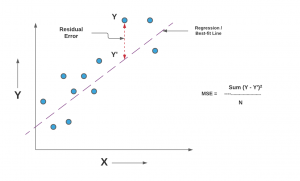
Mathematically, the MSE can be calculated as the average sum of the squared difference between the actual value and the predicted or estimated value represented by the regression model (line or plane). It is also termed as mean squared deviation (MSD). This is how it is represented mathematically:

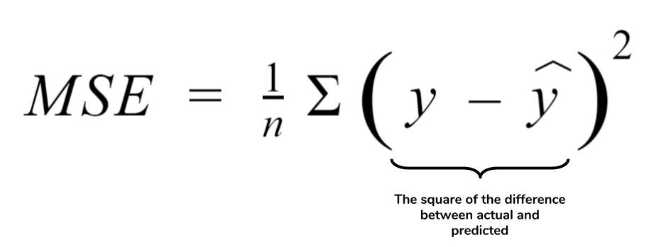
The value of MSE is always positive. A value close to zero will represent better quality of the estimator/predictor (regression model).

An MSE of zero (0) represents the fact that the predictor is a perfect predictor.

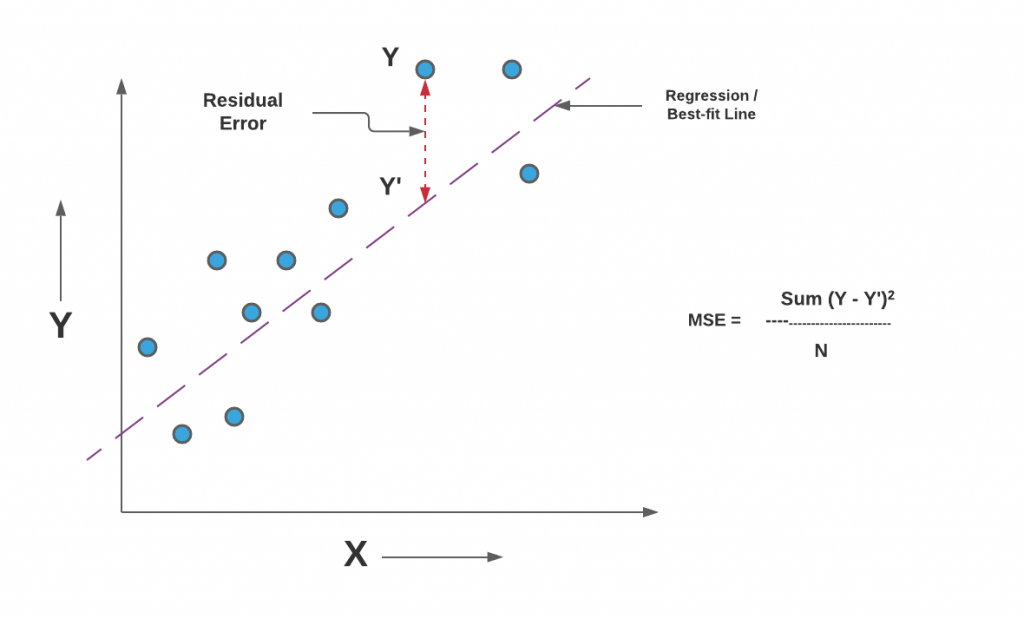
When you take a square root of MSE value, it becomes root mean squared error (RMSE). RMSE has also been termed root mean square deviation (RMSD). In the above equation, Y represents the actual value and the Y_hat represents the predicted value that could be found on the regression line or plane. Here is the diagrammatic representation of MSE for a simple linear or univariate regression model:

What is R-Squared?

R-Squared is the ratio of the sum of squares regression (SSR) and the sum of squares total (SST). Sum of Squares Regression (SSR) represents the total variation of all the predicted values found on the regression line or plane from the mean value of all the values of response variables. The sum of squares total (SST) represents the total variation of actual values from the mean value of all the values of response variables. R-squared value is used to measure the goodness of fit or best-fit line. The greater the value of R-Squared, the better is the regression model as most of the variation of actual values from the mean value get explained by the regression model. However, we need to take caution while relying on R-squared to assess the performance of the regression model. This is where the adjusted R-squared concept comes into the picture. This would be discussed in one of the later posts. R-Squared is also termed as the coefficient of determination. For the training dataset, the value of R-squared is bounded between 0 and 1, but it can become negative for the test dataset if the SSE is greater than SST. Greater the value of R-squared would also mean a smaller value of MSE. If the value of R-Squared becomes 1 (ideal world scenario), the model fits the data perfectly with a corresponding MSE = 0. As the value of R-squared increases and become close to 1, the value of MSE becomes close to 0.

Here is a visual representation to understand the concepts of R-Squared in a better manner.

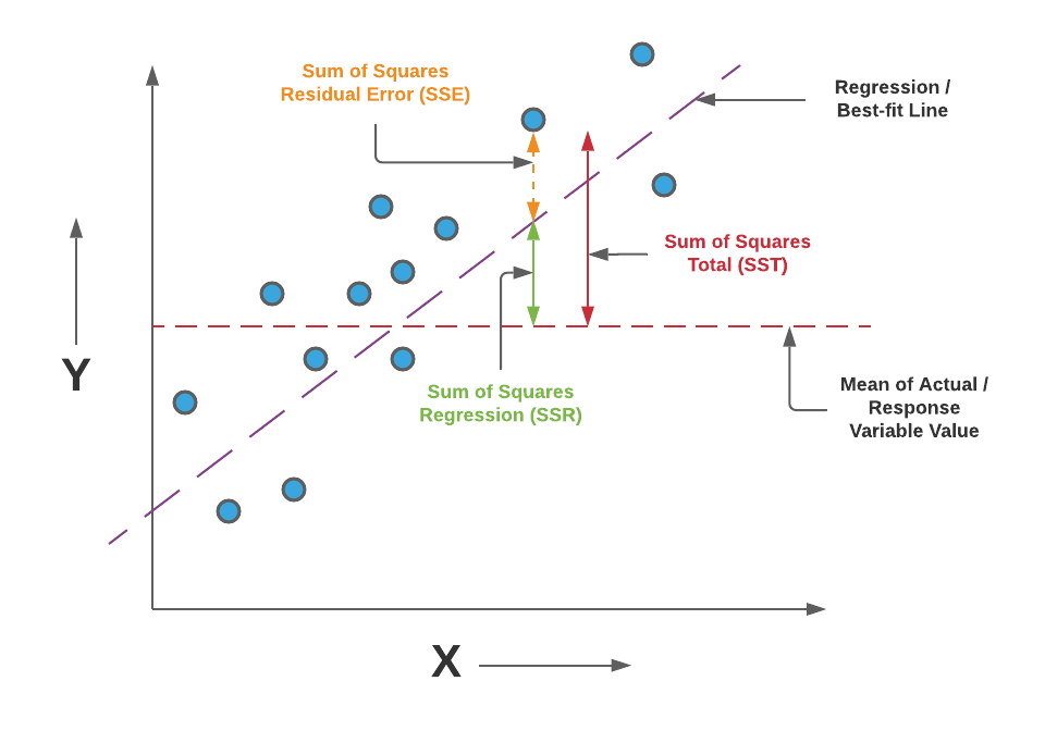
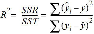
Pay attention to the diagram and note that the greater the value of SSR, the more is the variance covered by the regression / best fit line out of total variance (SST). R-Squared can also be represented using the following formula:

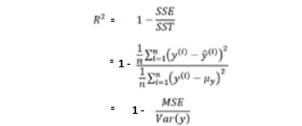
R-Squared = 1 – (SSE/SST)

Pay attention to the diagram and note that the smaller the value of SSE, the smaller is the value of (SSE/SST), and hence greater will be the value of R-Squared. Read further details on R-squared in this blog – R-squared/R2 in linear regression: Concepts, Examples

R-Squared can also be expressed as a function of mean squared error (MSE). The following equation represents the same. You may notice that as MSE increases, the value of R2 will decrease owing to the fact that the ratio of MSE and Var(y) will increase resulting in the decrease in the value of R2.

Difference between Mean Square Error & R-Squared

The similarity between mean-squared error and R-Squared is that they both are a type of metrics that are used for evaluating the performance of the linear regression models.

The difference is that MSE gets pronounced based on whether the data is scaled or not. For example, if the response variable is housing price in the multiple of 10K, MSE will be different (lower) than when the response variable such as housing pricing is not scaled (actual values). This is where R-Squared comes to the rescue. R-Squared is also termed the standardized version of MSE. R-squared represents the fraction of variance of the actual value of the response variable captured by the regression model rather than the MSE which captures the residual error.

MSE or R-Squared – Which one to Use?

It is recommended to use R-Squared or rather adjusted R-Squared for evaluating the model performance of the regression models. This is primarily because R-Squared captures the fraction of variance of actual values captured by the regression model and tends to give a better picture of the quality of the regression model. Also, MSE values differ based on whether the values of the response variable are scaled or not. A better measure instead of MSE is the root mean squared error (RMSE) which takes care of the fact related to whether the values of the response variable are scaled or not.

One can alternatively use MSE or R-Squared based on what is appropriate and the need of the hour. However, the disadvantage of using MSE than R-squared is that it will be difficult to gauge the performance of the model using MSE as the value of MSE can vary from 0 to any larger number. However, in the case of R-squared, the value is bounded between 0 and 1. A value of R-squared closer to 1 would mean that the regression model covers most part of the variance of the values of the response variable and can be termed as a good model. However, with the MSE value, depending on the scale of values of the response variable, the value will be different and hence, it would be difficult to assess for certain whether the regression model is good or otherwise.

MSE or R-Squared Python Code Example

Here is the python code representing how to calculate mean squared error or R-Squared value while working with regression models. Pay attention to some of the following in the code given below:

• Sklearn.metrics mean_squared_error and r2_score is used for measuring the MSE and R-Squared values. Input to this methods are actual values and predicted values.
• Sklearn Boston housing dataset is used for training a multiple linear regression model using Sklearn.linear_model LinearRegression

import pandas as pd
from sklearn.model_selection import train_test_split
from sklearn.preprocessing import StandardScaler
from sklearn.linear_model import LinearRegression
from sklearn.pipeline import make_pipeline
from sklearn.metrics import mean_squared_error, r2_score
from sklearn import datasets
#
# Load the Sklearn Boston Dataset
#
boston_ds = datasets.load_boston()
X = boston_ds.data
y = boston_ds.target
#
# Create a training and test split
#
X_train, X_test, y_train, y_test = train_test_split(X, y, test_size=0.3, random_state=42)
#
# Fit a pipeline using Training dataset and related labels
#
pipeline = make_pipeline(StandardScaler(), LinearRegression())
pipeline.fit(X_train, y_train)
#
# Calculate the predicted value for training and test dataset
#
y_train_pred = pipeline.predict(X_train)
y_test_pred = pipeline.predict(X_test)
#
# Mean Squared Error
#
print('MSE train: %.3f, test: %.3f' % (mean_squared_error(y_train, y_train_pred),
                mean_squared_error(y_test, y_test_pred)))
#
# R-Squared
#
print('R^2 train: %.3f, test: %.3f' % (r2_score(y_train, y_train_pred),
                r2_score(y_test, y_test_pred)))

Conclusions

Here is the summary of what you learned in this post regarding mean square error (MSE) and R-Squared and which one to use?

• MSE represents the residual error which is nothing but sum of squared difference between actual values and the predicted / estimated values divided by total number of records.
• R-Squared represents the fraction of variance captured by the regression model.
• The disadvantage of using MSE is that the value of MSE varies based on whether the values of response variable is scaled or not. If scaled, MSE will be lower than the unscaled values.