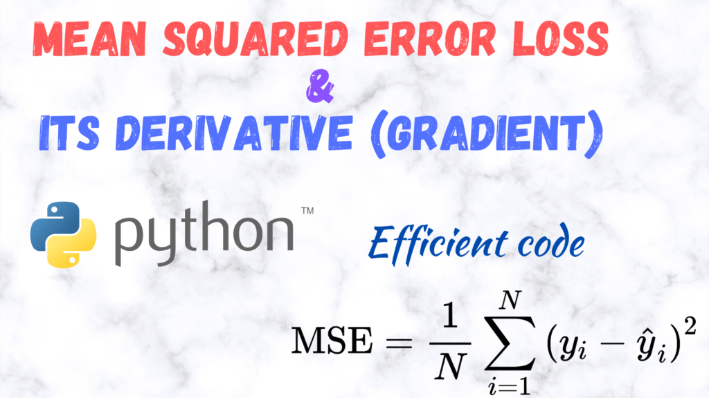
In this post, I show you how to implement the Mean Squared Error (MSE) Loss/Cost function as well as its derivative for Neural networks in Python. The function is meant for working with a batch of inputs, i.e., a batch of samples is provided at once.
The mathematical definition of the MSE loss function is
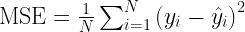
where  are the expected or target outputs (known beforehand),
  are the predicted outputs from the neural network, and
  is the number of samples.
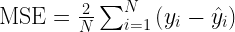
The derivative of the MSE loss function is:
Please note, that in the above definitions we are only considering a single output node. That is there is one output per sample.
But it is very common for neural networks to have more than one output node (multiple outputs) for a given input. In that case one has to average the squared error not only over the samples but also over the number of output nodes.
In this post I will only focus on this general case which means we would expect the predicted and target outputs to be 2D arrays, with nRows=nSamples, and nColumns=nOutput_Nodes. In other words, the rows correspond to outputs for different set of input samples, and the columns correspond to the outputs from the different output nodes.
Based on this we can implement the MSE loss function in Python as:
MSE loss simplest implementation
def MSE_loss(predictions, targets):
    """
    Computes Mean Squared error/loss between targets
    and predictions.
    Input: predictions (N, k) ndarray (N: no. of samples, k: no. of output nodes)
          targets (N, k) ndarray        (N: no. of samples, k: no. of output nodes)
    Returns: scalar
    Note: The averaging is only done over the output nodes and not over the samples in a batch.
    Therefore, to get an answer similar to PyTorch, one must divide the result by the batch size.
    """

    return np.sum((predictions-targets**2)/predictions.shape[1]
MSE loss derivative simplest implementation
def MSE_loss_grad(predictions, targets):
    """
    Computes mean squared error gradient between targets
    and predictions.
    Input: predictions (N, k) ndarray (N: no. of samples, k: no. of output nodes)
          targets (N, k) ndarray        (N: no. of samples, k: no. of output nodes)
    Returns: (N,k) ndarray
    Note: The averaging is only done over the output nodes and not over the samples in a batch.
    Therefore, to get an answer similar to PyTorch, one must divide the result by the batch size.
    """

    return 2*(predictions-targets)/predictions.shape[1]
The above functions return the MSE loss and its derivative respectively, only averaged over the output nodes. Averaging over the samples can then be done by simply dividing the result by nSamples as shown
average_MSE = MSE_loss(predictions, target)/predictions.shape[0]
average_MSE_grad = MSE_loss_grad(predictions, target)/predictions.shape[0]
These implementations can be further accelerated (sped-up) by using Numba (https://numba.pydata.org/). Numba is a Just-in-time (JIT) compiler that
translates a subset of Python and NumPy code into fast machine code.
To use numba, install it as:
pip install numba
Also, make sure that your numpy is compatible with Numba or not, although usually pip takes care of that. You can get the info here: https://pypi.org/project/numba/
Accelerating the above functions using Numba is quite simple. Just modify them in the following manner:
MSE loss NUMBA implementation
from numba import njit
@njit(cache=True,fastmath=True)
def MSE_loss(predictions, targets):
    """
    Computes Mean Squared error/loss between targets
    and predictions.
    Input: predictions (N, k) ndarray (N: no. of samples, k: no. of output nodes)
          targets (N, k) ndarray        (N: no. of samples, k: no. of output nodes)
    Returns: scalar
    Note: The averaging is only done over the output nodes and not over the samples in a batch.
    Therefore, to get an answer similar to PyTorch, one must divide the result by the batch size.
    """

    return np.sum((predictions-targets)**2)/predictions.shape[1]
NOTE: I noticed that the above implementation can be unstable and return erroneous results for very large arrays. Therefore, you can use the following even faster implementation with parallelization:
from numba import njit
@njit(cache=True,fastmath=False, parallel=True)
def MSE_loss(predictions, targets):
    """
    Computes Mean Squared error/loss between targets
    and predictions.
    Input: predictions (N, k) ndarray (N: no. of samples, k: no. of output nodes)
          targets (N, k) ndarray        (N: no. of samples, k: no. of output nodes)
    Returns: scalar
    Note: The averaging is only done over the output nodes and not over the samples in a batch.
    Therefore, to get an answer similar to PyTorch, one must divide the result by the batch size.
    """
    loss = 0.0
    for i in prange(predictions.shape[0]):
        for j in range(predictions.shape[1]):
            loss = loss + (predictions[i,j] - targets[i,j])**2
    # Average over number of output nodes
    loss = loss / predictions.shape[1]
    return loss
MSE loss derivative NUMBA implementation
from numba import njit
@njit(cache=True,fastmath=True)
def MSE_loss_grad(predictions, targets):
    """
    Computes mean squared error gradient between targets
    and predictions.
    Input: predictions (N, k) ndarray (N: no. of samples, k: no. of output nodes)
          targets (N, k) ndarray        (N: no. of samples, k: no. of output nodes)
    Returns: (N,k) ndarray
    Note: The averaging is only done over the output nodes and not over the samples in a batch.
    Therefore, to get an answer similar to PyTorch, one must divide the result by the batch size.
    """

    return 2*(predictions-targets)/predictions.shape[1]
This is quite fast and competitive with Tensorflow and PyTorch.
It is in fact also used in the CrysX-Neural Network library (crysx_nn)
Furthermore, the above implementations can also be accelerated using Cupy (CUDA).
CuPy is an open-source array library for GPU-accelerated computing with Python. CuPy utilizes CUDA Toolkit libraries to make full use of the GPU architecture.
The Cupy implementations look as follows:
def MSE_loss_cupy(predictions, targets):
    """
    Computes Mean Squared error/loss between targets
    and predictions.
    Input: predictions (N, k) ndarray (N: no. of samples, k: no. of output nodes)
          targets (N, k) ndarray        (N: no. of samples, k: no. of output nodes)
    Returns: scalar
    Note: The averaging is only done over the output nodes and not over the samples in a batch.
    Therefore, to get an answer similar to PyTorch, one must divide the result by the batch size.
    """

    return cp.sum((predictions-targets)**2)/predictions.shape[1]
def MSE_loss_grad_cupy(predictions, targets):
    """
    Computes mean squared error gradient between targets
    and predictions.
    Input: predictions (N, k) ndarray (N: no. of samples, k: no. of output nodes)
          targets (N, k) ndarray        (N: no. of samples, k: no. of output nodes)
    Returns: (N,k) ndarray
    Note: The averaging is only done over the output nodes and not over the samples in a batch.
    Therefore, to get an answer similar to PyTorch, one must divide the result by the batch size.
    """

    return 2*(predictions-targets)/predictions.shape[1]
The above code is also used in the crysx_nn library.
I hope you found this information useful.
If you did, then don’t forget to check out my other posts on Machine Learning and efficient implementations of activation/loss functions in Python.

Ph.D. researcher at Friedrich-Schiller University Jena, Germany. I’m a physicist specializing in computational material science. I write efficient codes for simulating light-matter interactions at atomic scales. I like to develop Physics, DFT, and Machine Learning related apps and software from time to time. Can code in most of the popular languages. I like to share my knowledge in Physics and applications using this Blog and a YouTube channel.
[wpedon id=»7041″ align=»center»]
Last Updated on June 21, 2020 by
Author(s): Pratik Shukla
Machine Learning
With Step-By-Step Mathematical Derivation

Index:
- Basics Of Gradient Descent.
- Basic Rules Of Derivation.
- Gradient Descent With One Variable.
- Gradient Descent With Two Variables.
- Gradient Descent For Mean Squared Error Function.
What is Gradient Descent?
Gradient Descent is a machine learning algorithm that operates iteratively to find the optimal values for its parameters. It takes into account, user-defined learning rate, and initial parameter values.
How does it work?
- Start with initial values.
- Calculate cost.
- Update values using the update function.
- Returns minimized cost for our cost function
Why do we need it?
Generally, what we do is, we find the formula that gives us the optimal values for our parameter. But in this algorithm, it finds the value by itself! Interesting, isn’t it?
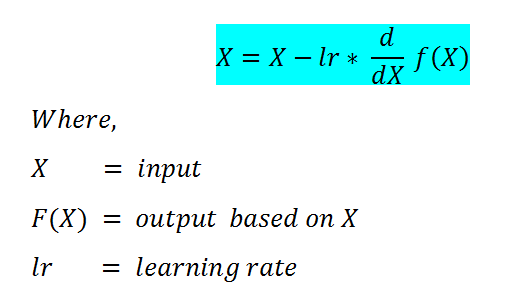
Formula:
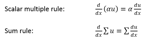
Some Basic Rules For Derivation:
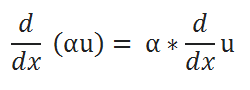
( A ) Scalar Multiple Rule:
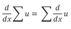
( B ) Sum Rule:
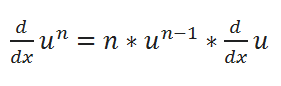
( C ) Power Rule:
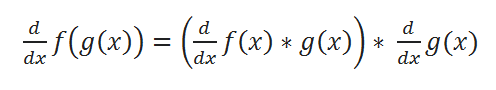
( D ) Chain Rule:
Let’s have a look at various examples to understand it better.
Gradient Descent Minimization — Single Variable:
We’re going to be using gradient descent to find θ that minimizes the cost. But let’s forget the Mean Squared Error (MSE) cost function for a moment and take a look at gradient descent function in general.
Now what we generally do is, find the best value of our parameters using some sort of simplification and make a function that will give us minimized cost. But here what we’ll do is take some default or random for our parameters and let our program run iteratively to find the minimized cost.
Let’s Explore It In-Depth:
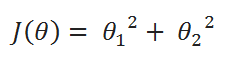
Let’s take a very simple function to begin with: J(θ) = θ², and our goal is to find the value of θ which minimizes J(θ).
From our cost function, we can clearly say that it will be minimum for θ= 0, but it won’t be so easy to derive such conclusions while working with some complex functions.
( A ) Cost function: We’ll try to minimize the value of this function.
( B ) Goal: To minimize the cost function.
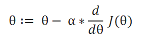
( C ) Update Function: Initially we take a random number for our parameters, which are not optimal. To make it optimal we have to update it at each iteration. This function takes care of it.
( D ) Learning rate: The descent speed.
( E ) Updating Parameters:
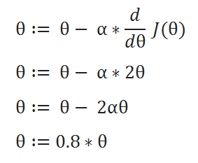
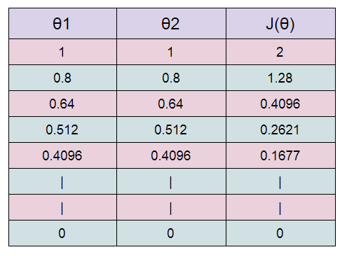
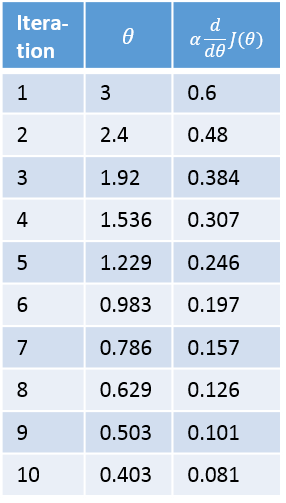
( F ) Table Generation:
Here we are stating with θ = 5.
keep in mind that here θ = 0.8*θ, for our learning rate and cost function.
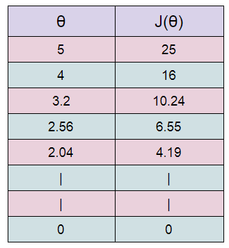
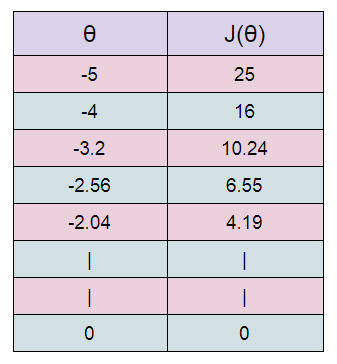
Here we can see that as our θ is decreasing the cost value is also decreasing. We just have to find the optimal value for it. To find the optimal value we have to do perform many iterations. The more the iterations, the more optimal value we get!
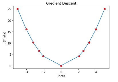
( G ) Graph: We can plot the graph of the above points.
Cost Function Derivative:
Why does the gradient descent use the derivative of the cost function? We want our cost function to be minimum, right? Minimizing the cost function simply gives us a lower error rate in predicting values. Ideally, we take the derivative of a function to 0 and find the parameters. Here we do the same thing but we start from a random number and try to minimize it iteratively.
The learning rate / ALPHA:
The learning rate gives us solid control over how large of steps we make. Selecting the right learning rate is a very critical task. If the learning rate is too high then you might overstep the minimum and diverge. For example, in the above example if we take alpha =2 then each iteration will take us away from the minimum. So we use small alpha values. But the only concern with using a small learning rate is we have to perform more iteration to reach the minimum cost value, this increases training time.
Convergence / Stopping gradient descent:
Note that in the above example the gradient descent will never actually converge to a minimum of theta= 0. Methods for deciding when to stop our iterations are beyond my level of expertise. But I can tell you that while doing assignments we can take a fixed number of iterations like 100 or 1000.
Gradient Descent — Multiple Variables:
Our ultimate goal is to find the parameters for MSE function, which includes multiple variables. So here we will discuss a cost function which as 2 variables. Understanding this will help us very much in our MSE Cost function.
Let’s take this function:
When there are multiple variables in the minimization objective, we have to define separate rules for update function. With more than one parameter in our cost function, we have to use partial derivative. Here I simplified the partial derivative process. Let’s have a look at this.
( A ) Cost Function:
( B ) Goal:
( C ) Update Rules:
( D ) Derivatives:
( E ) Update Values:
( F ) Learning Rate:
( G ) Table:
Starting with θ1 =1 ,θ2 =1. And then updating the value using update functions.
( H ) Graph:
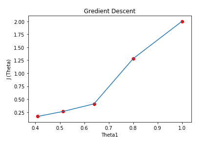
Here we can see that as we increase our number of iterations, our cost value is going down.
Note that while implementing the program in python the new values must not be updated until we find new values for both θ1 and θ2. We clearly don’t want to use the new value of θ1 to be used in the old value of θ2.
Gradient Descent For Mean Squared Error:
Now that we know how to perform gradient descent on an equation with multiple variables, we can return to looking at gradient descent on our MSE cost function.
Let’s get started!
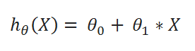
( A ) Hypothesis function:
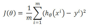
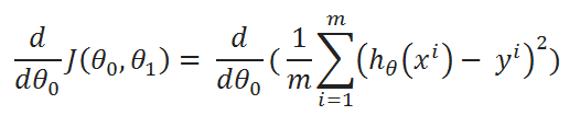
( B ) cost function:
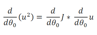
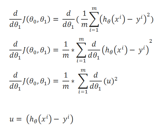
( C ) Find partial derivative of J(θ0,θ1) w.r.t to θ1:
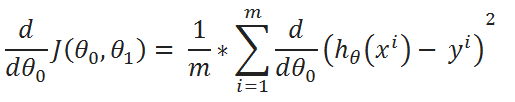
( D ) Simplify a little:
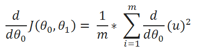
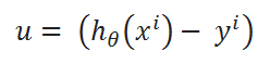
( E ) Define a variable u:
( F ) Value of u:
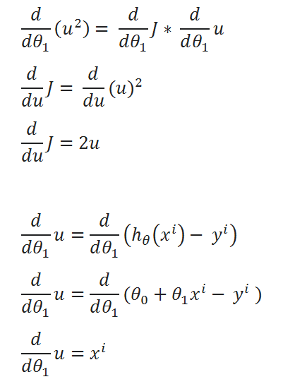
( G ) Finding partial derivative:
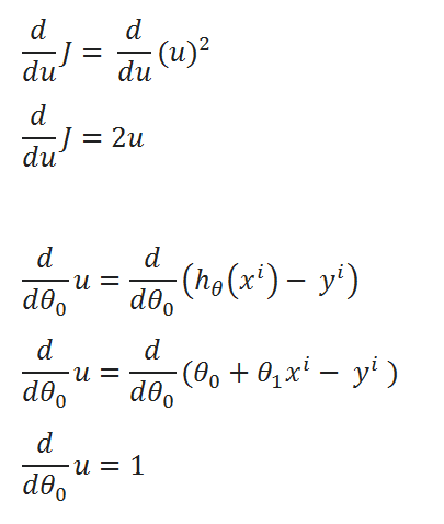
( H ) Rewriting the equations:
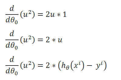
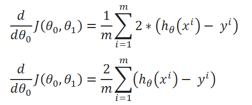
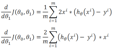
( I ) Merge all the calculated data:
( J ) Repeat the same process for derivation of J(θ0,θ1) w.r.t θ1:
( K ) Simplified calculations:
( L ) Combine all calculated Data:
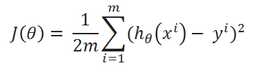
One Half Mean Squared Error :
We multiply our MSE cost function with 1/2, so that when we take the derivative the 2s cancel out. Multiplying the cost function by a scalar does not affect the location of the minimum, so we can get away with this.
Final :
( A ) Cost Function: One Half Mean Squared Error:
( B ) Goal:
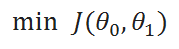
( C ) Update Rule:
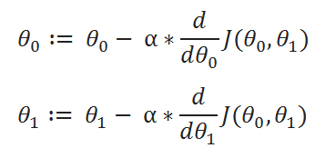
( D ) Derivatives:
So, that’s it. We finally made it!
Conclusion:
We are going to use the same method in various applications of machine learning algorithms. But at that time we are not going to go in this depth, we’re just going to use the final formula. But it’s always good to know how it’s derived!
Final Formula:
Is the concept lucid to you now? Please let me know by writing responses. If you enjoyed this article then hit the clap icon.
If you have any additional confusions, feel free to contact me. [email protected]
![]()
Gradient Descent Algorithm Explained was originally published in Towards AI — Multidisciplinary Science Journal on Medium, where people are continuing the conversation by highlighting and responding to this story.
Published via Towards AI
04 Mar 2014
Andrew Ng’s course on Machine Learning at Coursera provides an excellent explanation of gradient descent for linear regression. To really get a strong grasp on it, I decided to work through some of the derivations and some simple examples here.
This material assumes some familiarity with linear regression, and is primarily intended to provide additional insight into the gradient descent technique, not linear regression in general.
I am making use of the same notation as the Coursera course, so it will be most helpful for students of that course.
For linear regression, we have a linear hypothesis function, ( h(x) = theta_0 + theta_1 x ). We want to find the values of ( theta_0 ) and ( theta_1 ) which provide the best fit of our hypothesis to a training set. The training set examples are labeled ( x, y ), where ( x ) is the input value and ( y ) is the output. The ith training example is labeled as ( x^{(i)}, y^{(i)} ). Do not confuse this as an exponent! It just means that this is the ith training example.
MSE Cost Function
The cost function ( J ) for a particular choice of parameters ( theta ) is the mean squared error (MSE):

Where the variables used are:

The MSE measures the average amount that the model’s predictions vary from the correct values, so you can think of it as a measure of the model’s performance on the training set. The cost is higher when the model is performing poorly on the training set. The objective of the learning algorithm, then, is to find the parameters ( theta ) which give the minimum possible cost ( J ).
This minimization objective is expressed using the following notation, which simply states that we want to find the ( theta ) which minimizes the cost ( J(theta) ).

Gradient Descent Minimization — Single Variable Example
We’re going to be using gradient descent to find ( theta ) that minimizes the cost. But let’s forget the MSE cost function for a moment and look at gradient descent as a minimization technique in general.
Let’s take the much simpler function ( J(theta) = {theta}^2 ), and let’s say we want to find the value of ( theta ) which minimizes ( J(theta) ).
Gradient descent starts with a random value of ( theta ), typically ( theta = 0 ), but since ( theta = 0 ) is already the minimum of our function ( {theta}^2 ), let’s start with ( theta = 3 ).
Gradient descent is an iterative algorithm which we will run many times. On each iteration, we apply the following “update rule” (the := symbol means replace theta with the value computed on the right):

Alpha is a parameter called the learning rate which we’ll come back to, but for now we’re going to set it to 0.1. The derivative of ( J(theta) ) is simply ( 2theta ).

Below is a plot of our function, ( J(theta) ), and the value of ( theta ) over ten iterations of gradient descent.

Below is a table showing the value of theta prior to each iteration, and the update amounts.
Cost Function Derivative
Why does gradient descent use the derivative of the cost function? Finding the slope of the cost function at our current ( theta ) value tells us two things.
The first is the direction to move theta in. When you look at the plot of a function, a positive slope means the function goes upward as you move right, so we want to move left in order to find the minimum. Similarly, a negative slope means the function goes downard towards the right, so we want to move right to find the minimum.
The second is how big of a step to take. If the slope is large we want to take a large step because we’re far from the minimum. If the slope is small we want to take a smaller step. Note in the example above how gradient descent takes increasingly smaller steps towards the minimum with each iteration.
The Learning Rate — Alpha
The learning rate gives the engineer some additional control over how large of steps we make.
Selecting the right learning rate is critical. If the learning rate is too large, you can overstep the minimum and even diverge. For example, think through what would happen in the above example if we used a learning rate of 2. Each iteration would take us farther away from the minimum!
The only concern with using too small of a learning rate is that you will need to run more iterations of gradient descent, increasing your training time.
Convergence / Stopping Gradient Descent
Note in the above example that gradient descent will never actually converge on the minimum, ( theta = 0 ). Methods for deciding when to stop gradient descent are beyond my level of expertise, but I can tell you that when gradient descent is used in the assignments in the Coursera course, gradient descent is run for a large, fixed number of iterations (for example, 100 iterations), with no test for convergence.
Gradient Descent — Multiple Variables Example
The MSE cost function includes multiple variables, so let’s look at one more simple minimization example before going back to the cost function.
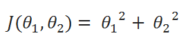
Let’s take the function:
[J(theta) = {theta_1}^2 + {theta_2}^2]
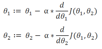
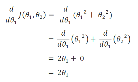
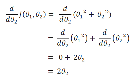
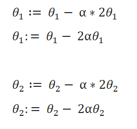
When there are multiple variables in the minimization objective, gradient descent defines a separate update rule for each variable. The update rule for ( theta_1 ) uses the partial derivative of ( J ) with respect to ( theta_1 ). A partial derivative just means that we hold all of the other variables constant–to take the partial derivative with respect to ( theta_1 ), we just treat ( theta_2 ) as a constant. The update rules are in the table below, as well as the math for calculating the partial derivatives. Make sure you work through those; I wrote out the derivation to make it easy to follow.

Note that when implementing the update rule in software, ( theta_1 ) and ( theta_2 ) should not be updated until after you have computed the new values for both of them. Specifically, you don’t want to use the new value of ( theta_1 ) to calculate the new value of ( theta_2 ).
Gradient Descent of MSE
Now that we know how to perform gradient descent on an equation with multiple variables, we can return to looking at gradient descent on our MSE cost function.
The MSE cost function is labeled as equation [1.0] below. Taking the derivative of this equation is a little more tricky. The key thing to remember is that x and y are not variables for the sake of the derivative. Rather, they represent a large set of constants (your training set). So when taking the derivative of the cost function, we’ll treat x and y like we would any other constant.
Once again, our hypothesis function for linear regression is the following:
[h(x) = theta_0 + theta_1 x]
I’ve written out the derivation below, and I explain each step in detail further down.
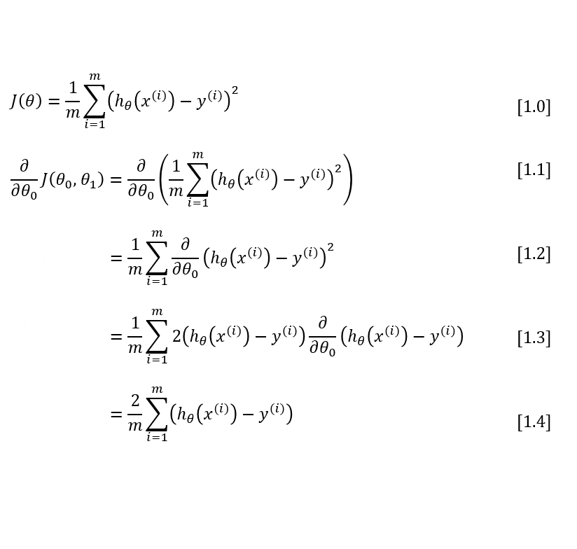
To move from equation [1.1] to [1.2], we need to apply two basic derivative rules:
Moving from [1.2] to [1.3], we apply both the power rule and the chain rule:


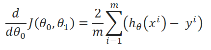
Finally, to go from [1.3] to [1.4], we must evaluate the partial derivative as follows. Recall again that when taking this partial derivative all letters except ( theta_0 ) are treated as constants ( ( theta_1 ), ( x ), and ( y )).

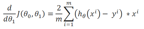
Equation [1.4] gives us the partial derivative of the MSE cost function with respect to one of the variables, ( theta_0 ). Now we must also take the partial derivative of the MSE function with respect to ( theta_1 ). The only difference is in the final step, where we take the partial derivative of the error:

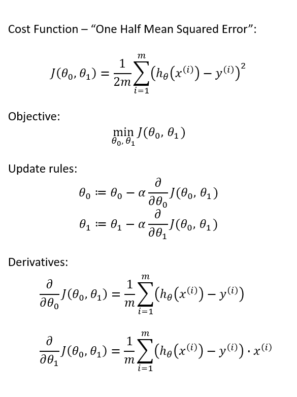
One Half Mean Squared Error
In Andrew Ng’s Machine Learning course, there is one small modification to this derivation. We multiply our MSE cost function by 1/2 so that when we take the derivative, the 2s cancel out. Multiplying the cost function by a scalar does not affect the location of its minimum, so we can get away with this.
Alternatively, you could think of this as folding the 2 into the learning rate. It makes sense to leave the 1/m term, though, because we want the same learning rate (alpha) to work for different training set sizes (m).
Final Update Rules
Altogether, we have the following definition for gradient descent over our cost function.
Training Set Statistics
Note that each update of the theta variables is averaged over the training set. Every training example suggests its own modification to the theta values, and then we take the average of these suggestions to make our actual update.
This means that the statistics of your training set are being taken into account during the learning process. An outlier training example (or even a mislabeled / corrupted example) is going to have less influence over the final weights because it is one voice versus many.
Функции активации
сигмовидная
σ(x) = 1/(1+e⁻ˣ)
- классическая функция активации для логистической регрессии
- сжать значения до [0, 1]
- Устарело в Pytorch 1.8.1:
torch.nn.functional.sigmoid - Вместо этого используйте
torch.sigmoid()
import torch

# import torch.nn.functional as F  # deprecated for sigmoid

# sigmoid
print("sigmoid function")
z = torch.linspace(-100, 100, 10)
print(z)
print(torch.sigmoid(z))  # value range [0,1]
- Нахождение градиента для сигмовидной функции: градиент может быть представлен самим σ, поэтому он требует меньше вычислительных ресурсов.

Преимущества:
- σ известно, поэтому не нужно искать производную, более эффективную
Недостаток:
- Когда x->∞, градиент ->0, очень небольшое обновление до w и b
Тан
tanh(x) = (eˣ-e⁻ˣ)/(eˣ+e⁻ˣ)=2*сигмоид(2x)-1
- Обычно используется в РНН
- Это преобразование сигмовидной функции
- сжать значение до [-1, 1]
- Градиент tanh(x) = 1-tanh²(x)
# tanh
print("ntanh function")
z = torch.linspace(-1, 1, 10)
print(torch.tanh(z))  # value range [-1, 1]
Релу
- Самый популярный для нейронной сети
- когда x‹0, градиент=0, когда x›0, градиент=x
# relu
print("nrelu function")
z = torch.linspace(-1, 1, 9)
print(z)
print(torch.relu(z))  # when z=0, torch.relu() gives 0
Функции потерь
Среднеквадратическая ошибка (MSE)
MSE=∑(y-(x*w+b))²
L2-норма = √(∑(y-(x*w+b))²) (RMS)
MSE = (L2-норма)²
import torch
import torch.nn.functional as F

# MSE
x=torch.ones(1)
w=torch.full([1], 2.)
mse=F.mse_loss(x*w, torch.ones(1))
print(mse)
Нахождение градиента для функции MSE
- если w не был определен правильно,
torch.autograd.grad()будет иметь ошибку - запустите
w.requires_grad_()и снова определите mse для обновления с новым w, прежде чем использовать autograd. - Последний _ в
w.requires_grad_()означает модификацию w на месте
# torch.autograd.grad(mse, [w])  # error

w.requires_grad_()  # need to add this line. The last _ means inplace
# torch.autograd.grad(mse, [w])  # error again

mse=F.mse_loss(x*w, torch.ones(1))  # need to update the loss function with updated x
print(mse)  # now mse contains information about gradient function

print(torch.autograd.grad(mse, [w]))
- Другой способ расчета градиента с помощью mse.backward()
# another way to calculate gradient
mse=F.mse_loss(x*w, torch.ones(1))
mse.backward()
print(w.grad)   # gradient is now saved in w
Софтмакс
- Отличие от сигмовидной: сжать значения до 0–1 И сумма всех членов = 1
- Это увеличит большую разницу и сожмет небольшую разницу между значениями:
b=torch.tensor([2,1,0.5])  # original ratio is [4:2:1]
b.requires_grad_()
p=F.softmax(b, dim=0)
print(p)
# OUTPUT: tensor([0.6285, 0.2312, 0.1402], grad_fn=<SoftmaxBackward>)
# ratio after softmax: [4.48:1.65:1]
bigger difference for big difference: 4.48/1.65=2.7
smaller difference for small difference: 1.65/1=1.65
Поиск градиента для функции softmax
- можно вычислить градиент только для скаляра, т.е. каждый элемент в softmax
- градиент для одного и того же термина +ve, для разных терминов -ve
# gradient for softmax
a=torch.rand(3)
a.requires_grad_()
print(a)

p=F.softmax(a, dim=0)
# p.backward()   # error, grad can only calculate for scalar outputs
print(torch.autograd.grad(p[1], [a], retain_graph=True))
print(torch.autograd.grad(p[2], [a])) # need to include retain_graph=True in previous step for running autograd again
# print(torch.autograd.grad(p[0], [a]))  # error here since previous step has no retain_graph
Чаевые для unknown
- для последовательного запуска torch.autograd необходимо установить
retain_graph=True, чтобы сохранить предыдущую информацию о градиенте - eg.
torch.autograd.grad(p[1], [a], retain_graph=True)
Ссылка
ссылка1