The mean squared error is a common way to measure the prediction accuracy of a model. In this tutorial, you’ll learn how to calculate the mean squared error in Python. You’ll start off by learning what the mean squared error represents. Then you’ll learn how to do this using Scikit-Learn (sklean), Numpy, as well as from scratch.
What is the Mean Squared Error
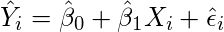
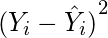
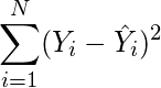
The mean squared error measures the average of the squares of the errors. What this means, is that it returns the average of the sums of the square of each difference between the estimated value and the true value.
The MSE is always positive, though it can be 0 if the predictions are completely accurate. It incorporates the variance of the estimator (how widely spread the estimates are) and its bias (how different the estimated values are from their true values).
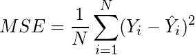
The formula looks like below:

Now that you have an understanding of how to calculate the MSE, let’s take a look at how it can be calculated using Python.
Interpreting the Mean Squared Error
The mean squared error is always 0 or positive. When a MSE is larger, this is an indication that the linear regression model doesn’t accurately predict the model.
An important piece to note is that the MSE is sensitive to outliers. This is because it calculates the average of every data point’s error. Because of this, a larger error on outliers will amplify the MSE.
There is no “target” value for the MSE. The MSE can, however, be a good indicator of how well a model fits your data. It can also give you an indicator of choosing one model over another.
Loading a Sample Pandas DataFrame
Let’s start off by loading a sample Pandas DataFrame. If you want to follow along with this tutorial line-by-line, simply copy the code below and paste it into your favorite code editor.
# Importing a sample Pandas DataFrame
import pandas as pd

df = pd.DataFrame.from_dict({
    'x': [1,2,3,4,5,6,7,8,9,10],
    'y': [1,2,2,4,4,5,6,7,9,10]})

print(df.head())
#    x  y
# 0  1  1
# 1  2  2
# 2  3  2
# 3  4  4
# 4  5  4
You can see that the editor has loaded a DataFrame containing values for variables x and y. We can plot this data out, including the line of best fit using Seaborn’s .regplot() function:
# Plotting a line of best fit
import seaborn as sns
import matplotlib.pyplot as plt
sns.regplot(data=df, x='x', y='y', ci=None)
plt.ylim(bottom=0)
plt.xlim(left=0)
plt.show()
This returns the following visualization:
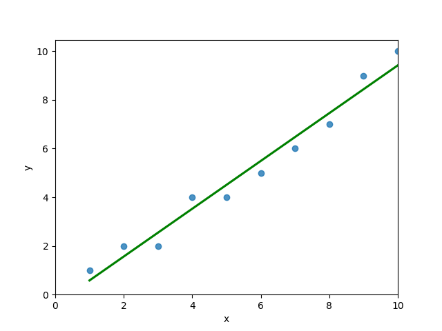
The mean squared error calculates the average of the sum of the squared differences between a data point and the line of best fit. By virtue of this, the lower a mean sqared error, the more better the line represents the relationship.
We can calculate this line of best using Scikit-Learn. You can learn about this in this in-depth tutorial on linear regression in sklearn. The code below predicts values for each x value using the linear model:
# Calculating prediction y values in sklearn
from sklearn.linear_model import LinearRegression

model = LinearRegression()
model.fit(df[['x']], df['y'])
y_2 = model.predict(df[['x']])
df['y_predicted'] = y_2
print(df.head())

# Returns:
#    x  y  y_predicted
# 0  1  1     0.581818
# 1  2  2     1.563636
# 2  3  2     2.545455
# 3  4  4     3.527273
# 4  5  4     4.509091
Calculating the Mean Squared Error with Scikit-Learn
The simplest way to calculate a mean squared error is to use Scikit-Learn (sklearn). The metrics module comes with a function, mean_squared_error() which allows you to pass in true and predicted values.
Let’s see how to calculate the MSE with sklearn:
# Calculating the MSE with sklearn
from sklearn.metrics import mean_squared_error
mse = mean_squared_error(df['y'], df['y_predicted'])
print(mse)

# Returns: 0.24727272727272714
This approach works very well when you’re already importing Scikit-Learn. That said, the function works easily on a Pandas DataFrame, as shown above.
In the next section, you’ll learn how to calculate the MSE with Numpy using a custom function.
Calculating the Mean Squared Error from Scratch using Numpy
Numpy itself doesn’t come with a function to calculate the mean squared error, but you can easily define a custom function to do this. We can make use of the subtract() function to subtract arrays element-wise.
# Definiting a custom function to calculate the MSE
import numpy as np

def mse(actual, predicted):
    actual = np.array(actual)
    predicted = np.array(predicted)
    differences = np.subtract(actual, predicted)
    squared_differences = np.square(differences)
    return squared_differences.mean()

print(mse(df['y'], df['y_predicted']))

# Returns: 0.24727272727272714
The code above is a bit verbose, but it shows how the function operates. We can cut down the code significantly, as shown below:
# A shorter version of the code above
import numpy as np

def mse(actual, predicted):
    return np.square(np.subtract(np.array(actual), np.array(predicted))).mean()

print(mse(df['y'], df['y_predicted']))

# Returns: 0.24727272727272714
Conclusion
In this tutorial, you learned what the mean squared error is and how it can be calculated using Python. First, you learned how to use Scikit-Learn’s mean_squared_error() function and then you built a custom function using Numpy.
The MSE is an important metric to use in evaluating the performance of your machine learning models. While Scikit-Learn abstracts the way in which the metric is calculated, understanding how it can be implemented from scratch can be a helpful tool.
Additional Resources
To learn more about related topics, check out the tutorials below:
- Pandas Variance: Calculating Variance of a Pandas Dataframe Column
- Calculate the Pearson Correlation Coefficient in Python
- How to Calculate a Z-Score in Python (4 Ways)
- Official Documentation from Scikit-Learn
In this article, we are going to learn how to calculate the mean squared error in python? We are using two python libraries to calculate the mean squared error. NumPy and sklearn are the libraries we are going to use here. Also, we will learn how to calculate without using any module.
MSE is also useful for regression problems that are normally distributed. It is the mean squared error. So the squared error between the predicted values and the actual values. The summation of all the data points of the square difference between the predicted and actual values is divided by the no. of data points.
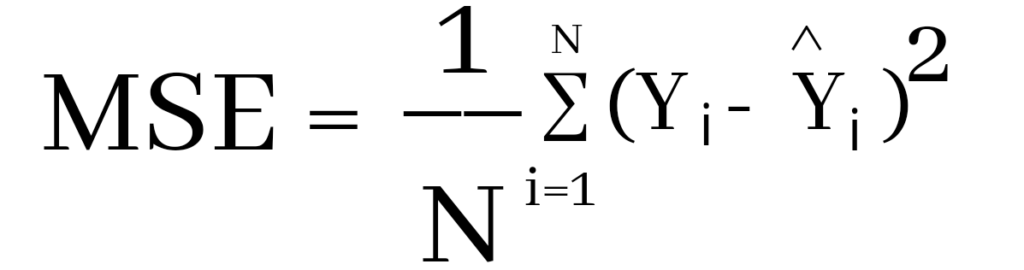
Where Yi and Ŷi represent the actual values and the predicted values, the difference between them is squared.
Derivation of Mean Squared Error
First to find the regression line for the values (1,3), (2,2), (3,6), (4,1), (5,5). The regression value for the value is y=1.6+0.4x. Next to find the new Y values. The new values for y are tabulated below.
| Given x value | Calculating y value | New y value |
|---|---|---|
| 1 | 1.6+0.4(1) | 2 |
| 2 | 1.6+0.4(2) | 2.4 |
| 3 | 1.6+0.4(3) | 2.8 |
| 4 | 1.6+0.4(4) | 3.2 |
| 5 | 1.6+0.4(5) | 3.6 |
Now to find the error ( Yi – Ŷi )
We have to square all the errors
By adding all the errors we will get the MSE
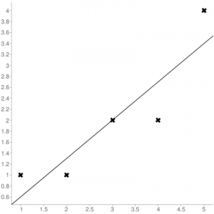
Line regression graph
Let us consider the values (1,3), (2,2), (3,6), (4,1), (5,5) to plot the graph.
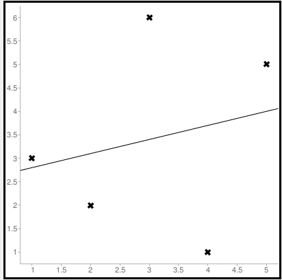
The straight line represents the predicted value in this graph, and the points represent the actual data. The difference between this line and the points is squared, known as mean squared error.
Also, Read | How to Calculate Square Root in Python
To get the Mean Squared Error in Python using NumPy
import numpy as np
true_value_of_y= [3,2,6,1,5]
predicted_value_of_y= [2.0,2.4,2.8,3.2,3.6]
MSE = np.square(np.subtract(true_value_of_y,predicted_value_of_y)).mean()
print(MSE)
Importing numpy library as np. Creating two variables. true_value_of_y holds an original value. predicted_value_of_y holds a calculated value. Next, giving the formula to calculate the mean squared error.
Output
3.6400000000000006
To get the MSE using sklearn
sklearn is a library that is used for many mathematical calculations in python. Here we are going to use this library to calculate the MSE
Syntax
sklearn.metrices.mean_squared_error(y_true, y_pred, *, sample_weight=None, multioutput='uniform_average', squared=True)
Parameters
- y_true – true value of y
- y_pred – predicted value of y
- sample_weight
- multioutput
- raw_values
- uniform_average
- squared
Returns
Mean squared error.
Code
from sklearn.metrics import mean_squared_error
true_value_of_y= [3,2,6,1,5]
predicted_value_of_y= [2.0,2.4,2.8,3.2,3.6]
mean_squared_error(true_value_of_y,predicted_value_of_y)
print(mean_squared_error(true_value_of_y,predicted_value_of_y))
From sklearn.metrices library importing mean_squared_error. Creating two variables. true_value_of_y holds an original value. predicted_value_of_y holds a calculated value. Next, giving the formula to calculate the mean squared error.
Output
3.6400000000000006
Calculating Mean Squared Error Without Using any Modules
true_value_of_y = [3,2,6,1,5]
predicted_value_of_y = [2.0,2.4,2.8,3.2,3.6]
summation_of_value = 0
n = len(true_value_of_y)
for i in range (0,n):
  difference_of_value = true_value_of_y[i] - predicted_value_of_y[i]
  squared_difference = difference_of_value**2
  summation_of_value = summation_of_value + squared_difference
MSE = summation_of_value/n
print ("The Mean Squared Error is: " , MSE)
Declaring the true values and the predicted values to two different variables. Initializing the variable summation_of_value is zero to store the values. len() function is useful to check the number of values in true_value_of_y. Creating for loop to iterate. Calculating the difference between true_value and the predicted_value. Next getting the square of the difference. Adding all the squared differences, we will get the MSE.
Output
The Mean Squared Error is: 3.6400000000000006
Calculate Mean Squared Error Using Negative Values
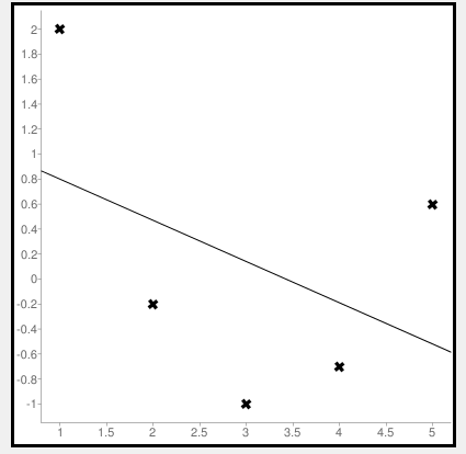
Now let us consider some negative values to calculate MSE. The values are (1,2), (3,-1), (5,0.6), (4,-0.7), (2,-0.2). The regression line equation is y=1.13-0.33x
The line regression graph for this value is:
New y values for this will be:
| Given x value | Calculating y value | New y value |
|---|---|---|
| 1 | 1.13-033(1) | 0.9 |
| 3 | 1.13-033(3) | 0.1 |
| 5 | 1.13-033(5) | -0.4 |
| 4 | 1.13-033(4) | -0.1 |
| 2 | 1.13-033(2) | 0.6 |
Code
>>> from sklearn.metrics import mean_squared_error
>>> y_true = [2,-1,0.6,-0.7,-0.2]
>>> y_pred = [0.9,0.1,-0.4,-0.1,0.6]
>>> mean_squared_error(y_true, y_pred)
First, importing a module. Declaring values to the variables. Here we are using negative value to calculate. Using the mean_squared_error module, we are calculating the MSE.
Output
0.884
Bonus: Gradient Descent
Gradient Descent is used to find the local minimum of the functions. In this case, the functions need to be differentiable. The basic idea is to move in the direction opposite from the derivate at any point.
The following code works on a set of values that are available on the Github repository.
Code:
#!/usr/bin/python
# -*- coding: utf-8 -*-
from numpy import *


def compute_error(b, m, points):
    totalError = 0
    for i in range(0, len(points)):
        x = points[i, 0]
        y = points[i, 1]
        totalError += (y - (m * x + b)) ** 2
    return totalError / float(len(points))


def gradient_step(
    b_current,
    m_current,
    points,
    learningRate,
    ):
    b_gradient = 0
    m_gradient = 0
    N = float(len(points))
    for i in range(0, len(points)):
        x = points[i, 0]
        y = points[i, 1]
        b_gradient += -(2 / N) * (y - (m_current * x + b_current))
        m_gradient += -(2 / N) * x * (y - (m_current * x + b_current))
    new_b = b_current - learningRate * b_gradient
    new_m = m_current - learningRate * m_gradient
    return [new_b, new_m]


def gradient_descent_runner(
    points,
    starting_b,
    starting_m,
    learning_rate,
    iterations,
    ):
    b = starting_b
    m = starting_m
    for i in range(iterations):
        (b, m) = gradient_step(b, m, array(points), learning_rate)
    return [b, m]


def main():
    points = genfromtxt('data.csv', delimiter=',')
    learning_rate = 0.00001
    initial_b = 0
    initial_m = 0
    iterations = 10000
    print('Starting gradient descent at b = {0}, m = {1}, error = {2}'.format(initial_b,
            initial_m, compute_error(initial_b, initial_m, points)))
    print('Running...')
    [b, m] = gradient_descent_runner(points, initial_b, initial_m,
            learning_rate, iterations)
    print('After {0} iterations b = {1}, m = {2}, error = {3}'.format(iterations,
            b, m, compute_error(b, m, points)))


if __name__ == '__main__':
    main()
Output:
Starting gradient descent at b = 0, m = 0, error = 5671.844671124282
Running...
After 10000 iterations b = 0.11558415090685024, m = 1.3769012288001614, error = 212.26220312358794
1. What is the pip command to install numpy?
pip install numpy
2. What is the pip command to install sklearn.metrices library?
pip install sklearn
3. What is the expansion of MSE?
The expansion of MSE is Mean Squared Error.
Conclusion
In this article, we have learned about the mean squared error. It is effortless to calculate. This is useful for loss function for least squares regression. The formula for the MSE is easy to memorize. We hope this article is handy and easy to understand.
Содержание
- Как рассчитать среднеквадратичную ошибку (MSE) в Python
- Как рассчитать MSE в Python
- How to Calculate Mean Squared Error (MSE) in Python
- Mean Squared Error Formula
- pip install numpy
- How to Calculate MSE in Python
- Example 1 – Mean Squared Error Calculation
- Example 2 – Mean Squared Error Calculation
- Conclusion
- How to Calculate Mean Squared Error in Python
- What is the Mean Squared Error
- Interpreting the Mean Squared Error
- Loading a Sample Pandas DataFrame
- Calculating the Mean Squared Error with Scikit-Learn
- Calculating the Mean Squared Error from Scratch using Numpy
- Conclusion
- Additional Resources
- Python | Mean Squared Error
- How To Calculate Mean Squared Error In Python
- Formula to calculate mean squared error
- Derivation of Mean Squared Error
- Line regression graph
- To get the Mean Squared Error in Python using NumPy
- To get the MSE using sklearn
- Syntax
- Parameters
- Returns
- Calculating Mean Squared Error Without Using any Modules
- Calculate Mean Squared Error Using Negative Values
- Bonus: Gradient Descent
Как рассчитать среднеквадратичную ошибку (MSE) в Python
Среднеквадратическая ошибка (MSE) — это распространенный способ измерения точности предсказания модели. Он рассчитывается как:
MSE = (1/n) * Σ(фактическое – прогноз) 2
- Σ — причудливый символ, означающий «сумма».
- n – размер выборки
- фактический – фактическое значение данных
- прогноз – прогнозируемое значение данных
Чем ниже значение MSE, тем лучше модель способна точно предсказывать значения.
Как рассчитать MSE в Python
Мы можем создать простую функцию для вычисления MSE в Python:
Затем мы можем использовать эту функцию для вычисления MSE для двух массивов: одного, содержащего фактические значения данных, и другого, содержащего прогнозируемые значения данных.
Среднеквадратическая ошибка (MSE) для этой модели оказывается равной 17,0 .
На практике среднеквадратическая ошибка (RMSE) чаще используется для оценки точности модели. Как следует из названия, это просто квадратный корень из среднеквадратичной ошибки.
Мы можем определить аналогичную функцию для вычисления RMSE:
Затем мы можем использовать эту функцию для вычисления RMSE для двух массивов: одного, содержащего фактические значения данных, и другого, содержащего прогнозируемые значения данных.
Среднеквадратическая ошибка (RMSE) для этой модели оказывается равной 4,1231 .
Источник
How to Calculate Mean Squared Error (MSE) in Python
Mean squared error (MSE) of an estimator measures the average of the squared errors, it means averages squared difference between the actual and estimated value.
MSE is almost positive because MSE of an estimator does not account for information that could produce more accurate estimate.
In statistical modelling, MSE is defined as the difference between actual values and predicted values by the model and used to determine prediction accuracy of a model.
In this tutorial, we will discuss about how to calculate mean squared error (MSE) in python.
Mean Squared Error Formula
The mean squared error (MSE) formula is defined as follows:
n = sample data points
y – actual size
y^ – predictive values
MSE is the means of squares of the errors ( yi – yi^) 2 .
We will be using numpy library to generate actual and predication values.
As there is no in built function available in python to calculate mean squared error (MSE), we will write simple function for calculation as per mean squared error formula.
pip install numpy
If you don’t have numpy package installed on your system, use below command in command prompt
How to Calculate MSE in Python
Lets understand with examples about how to calculate mean squared error (MSE) in python with given below python code
In the above example, we have created actual and prediction array with the help of numpy package array function.
We have written simple function mse() as per mean squared error formula which takes two parameters actual and prediction data array. It calculates mean of the squares of (actual – prediction) using numpy packages square and mean function.
Above code returns mean squared error (MSE) value for given actual and prediction model is 3.42857
Lets check out Mean squared Error (MSE) calculation with few other examples
Info Tip: How to calculate SMAPE in Python!
Example 1 – Mean Squared Error Calculation
Lets assume we have actual and forecast dataset as below
Calculate MSE for given model.
Here, again we will be using numpy package to create actual and prediction array and simple mse() function for mean squared error calculation in python code as below
Above code returns mean squared error (MSE) for given actual and prediction dataset is 1.3
Info Tip: How to calculate rolling correlation in Python!
Example 2 – Mean Squared Error Calculation
Lets take another example with below actual and prediction data values
actual = [-2,-1,1,4]
prediction = [-3,-1,2,3]
Calcualte MSE for above model.
Using below python code, lets calculate MSE
Above code returns mean squared error (MSE) for given actual and prediction dataset is 0.75 . It means it has less squared error and hence this model predicts more accuracy.
Info Tip: How to calculate z score in Python!
Conclusion
I hope, you may find how to calculate MSE in python tutorial with step by step illustration of examples educational and helpful.
Mean squared error (MSE) measures the prediction accuracy of model. Minimizing MSE is key criterion in selecting estimators.
Источник
How to Calculate Mean Squared Error in Python
The mean squared error is a common way to measure the prediction accuracy of a model. In this tutorial, you’ll learn how to calculate the mean squared error in Python. You’ll start off by learning what the mean squared error represents. Then you’ll learn how to do this using Scikit-Learn (sklean), Numpy, as well as from scratch.
Table of Contents
What is the Mean Squared Error
The mean squared error measures the average of the squares of the errors. What this means, is that it returns the average of the sums of the square of each difference between the estimated value and the true value.
The MSE is always positive, though it can be 0 if the predictions are completely accurate. It incorporates the variance of the estimator (how widely spread the estimates are) and its bias (how different the estimated values are from their true values).
The formula looks like below:
Now that you have an understanding of how to calculate the MSE, let’s take a look at how it can be calculated using Python.
Interpreting the Mean Squared Error
The mean squared error is always 0 or positive. When a MSE is larger, this is an indication that the linear regression model doesn’t accurately predict the model.
An important piece to note is that the MSE is sensitive to outliers. This is because it calculates the average of every data point’s error. Because of this, a larger error on outliers will amplify the MSE.
There is no “target” value for the MSE. The MSE can, however, be a good indicator of how well a model fits your data. It can also give you an indicator of choosing one model over another.
Loading a Sample Pandas DataFrame
Let’s start off by loading a sample Pandas DataFrame. If you want to follow along with this tutorial line-by-line, simply copy the code below and paste it into your favorite code editor.
You can see that the editor has loaded a DataFrame containing values for variables x and y . We can plot this data out, including the line of best fit using Seaborn’s .regplot() function:
This returns the following visualization:
Plotting a line of best fit to help visualize mean squared error in Python
The mean squared error calculates the average of the sum of the squared differences between a data point and the line of best fit. By virtue of this, the lower a mean sqared error, the more better the line represents the relationship.
We can calculate this line of best using Scikit-Learn. You can learn about this in this in-depth tutorial on linear regression in sklearn. The code below predicts values for each x value using the linear model:
Calculating the Mean Squared Error with Scikit-Learn
The simplest way to calculate a mean squared error is to use Scikit-Learn (sklearn). The metrics module comes with a function, mean_squared_error() which allows you to pass in true and predicted values.
Let’s see how to calculate the MSE with sklearn:
This approach works very well when you’re already importing Scikit-Learn. That said, the function works easily on a Pandas DataFrame, as shown above.
In the next section, you’ll learn how to calculate the MSE with Numpy using a custom function.
Calculating the Mean Squared Error from Scratch using Numpy
Numpy itself doesn’t come with a function to calculate the mean squared error, but you can easily define a custom function to do this. We can make use of the subtract() function to subtract arrays element-wise.
The code above is a bit verbose, but it shows how the function operates. We can cut down the code significantly, as shown below:
Conclusion
In this tutorial, you learned what the mean squared error is and how it can be calculated using Python. First, you learned how to use Scikit-Learn’s mean_squared_error() function and then you built a custom function using Numpy.
The MSE is an important metric to use in evaluating the performance of your machine learning models. While Scikit-Learn abstracts the way in which the metric is calculated, understanding how it can be implemented from scratch can be a helpful tool.
Additional Resources
To learn more about related topics, check out the tutorials below:
Источник
Python | Mean Squared Error
The Mean Squared Error (MSE) or Mean Squared Deviation (MSD) of an estimator measures the average of error squares i.e. the average squared difference between the estimated values and true value. It is a risk function, corresponding to the expected value of the squared error loss. It is always non – negative and values close to zero are better. The MSE is the second moment of the error (about the origin) and thus incorporates both the variance of the estimator and its bias.
Steps to find the MSE
- Find the equation for the regression line.
(1) 
Insert X values in the equation found in step 1 in order to get the respective Y values i.e.
(2) 
(3) 
Square the errors found in step 3.
(4) 
Sum up all the squares.
(5) 
(6) 
Example:
Consider the given data points: (1,1), (2,1), (3,2), (4,2), (5,4)
You can use this online calculator to find the regression equation / line.
Regression line equation: Y = 0.7X – 0.1
| X | Y |  |
|---|---|---|
| 1 | 1 | 0.6 |
| 2 | 1 | 1.29 |
| 3 | 2 | 1.99 |
| 4 | 2 | 2.69 |
| 5 | 4 | 3.4 |
Now, using formula found for MSE in step 6 above, we can get MSE = 0.21606
Источник
How To Calculate Mean Squared Error In Python
In this article, we are going to learn how to calculate the mean squared error in python? We are using two python libraries to calculate the mean squared error. NumPy and sklearn are the libraries we are going to use here. Also, we will learn how to calculate without using any module.
MSE is also useful for regression problems that are normally distributed. It is the mean squared error. So the squared error between the predicted values and the actual values. The summation of all the data points of the square difference between the predicted and actual values is divided by the no. of data points.
Formula to calculate mean squared error
Where Yi and Ŷi represent the actual values and the predicted values, the difference between them is squared.
Derivation of Mean Squared Error
First to find the regression line for the values (1,3), (2,2), (3,6), (4,1), (5,5). The regression value for the value is y=1.6+0.4x. Next to find the new Y values. The new values for y are tabulated below.
| Given x value | Calculating y value | New y value |
|---|---|---|
| 1 | 1.6+0.4(1) | 2 |
| 2 | 1.6+0.4(2) | 2.4 |
| 3 | 1.6+0.4(3) | 2.8 |
| 4 | 1.6+0.4(4) | 3.2 |
| 5 | 1.6+0.4(5) | 3.6 |
Now to find the error ( Yi – Ŷi )
We have to square all the errors
By adding all the errors we will get the MSE
Line regression graph
Let us consider the values (1,3), (2,2), (3,6), (4,1), (5,5) to plot the graph.
The straight line represents the predicted value in this graph, and the points represent the actual data. The difference between this line and the points is squared, known as mean squared error.
To get the Mean Squared Error in Python using NumPy
Importing numpy library as np. Creating two variables. true_value_of_y holds an original value. predicted_value_of_y holds a calculated value. Next, giving the formula to calculate the mean squared error.
Output
To get the MSE using sklearn
sklearn is a library that is used for many mathematical calculations in python. Here we are going to use this library to calculate the MSE
Syntax
Parameters
- y_true – true value of y
- y_pred – predicted value of y
- sample_weight
- multioutput
- raw_values
- uniform_average
- squared
Returns
Mean squared error.
From sklearn.metrices library importing mean_squared_error. Creating two variables. true_value_of_y holds an original value. predicted_value_of_y holds a calculated value. Next, giving the formula to calculate the mean squared error.
Output
Calculating Mean Squared Error Without Using any Modules
Declaring the true values and the predicted values to two different variables. Initializing the variable summation_of_value is zero to store the values. len() function is useful to check the number of values in true_value_of_y. Creating for loop to iterate. Calculating the difference between true_value and the predicted_value. Next getting the square of the difference. Adding all the squared differences, we will get the MSE.
Output
Calculate Mean Squared Error Using Negative Values
Now let us consider some negative values to calculate MSE. The values are (1,2), (3,-1), (5,0.6), (4,-0.7), (2,-0.2). The regression line equation is y=1.13-0.33x
The line regression graph for this value is:
New y values for this will be:
| Given x value | Calculating y value | New y value |
|---|---|---|
| 1 | 1.13-033(1) | 0.9 |
| 3 | 1.13-033(3) | 0.1 |
| 5 | 1.13-033(5) | -0.4 |
| 4 | 1.13-033(4) | -0.1 |
| 2 | 1.13-033(2) | 0.6 |
First, importing a module. Declaring values to the variables. Here we are using negative value to calculate. Using the mean_squared_error module, we are calculating the MSE.
Output
Bonus: Gradient Descent
Gradient Descent is used to find the local minimum of the functions. In this case, the functions need to be differentiable. The basic idea is to move in the direction opposite from the derivate at any point.
The following code works on a set of values that are available on the Github repository.
Источник