Some of the topics which have been explained are as follows:
-
Definitions of accuracy
-
Accuracy and Precision With Respect to Physics
-
Accuracy and Precision in the Context of Errors
-
Accuracy
-
Precision
-
Error
-
Uncertainty
Precision is a depiction of irregular errors, a proportion of statistical changeability.
Accuracy, However, Has Two Definitions
Usually, it is used to explain «it is a depiction of systematic errors, a proportion of statistical bias (on the researcher’s or the experimenter’s part); as these are causative of a distinction between an outcome and an «actual or true» value, ISO calls this trueness. On the other hand, ISO characterizes accuracy as portraying a blend of the two kinds of observational error above (irregular and methodical), so high accuracy requires both high precision and high certainty.
In the least difficult terms, given a lot of information focuses on repetitive measurements of a similar quantity or result, the set can be said to be exact if the values are near one another, while the set can be said to be accurate if their average is near the true value of the quantity being valued. In the first, common definition given above, the two ideas are autonomous of one another, so a specific arrangement of information can be said to be either accurate, or precise, or both, or neither of the two.
In the domains of science and engineering, the accuracy of an estimation framework is the degree of closeness of a quantity to that quantity’s actual or true value. The accuracy of an estimation framework, identified with reproducibility and repeatability, is the degree up to which repeated estimations under unaltered conditions demonstrate the equivalent results.
Although the two words accuracy and precision can be synonymous in everyday use, they are intentionally differentiated when used in the context of science and engineering. As mentioned earlier, an estimation framework can be accurate yet not precise, precise yet not accurate, neither or the other, or both. For instance, on the off chance that an investigation contains a systematic error, at that point expanding the sample size, for the most part, builds precision yet does not necessarily improve accuracy.
The outcome would be a consistent yet inaccurate series of results from the defective examination. Taking out the systematic error improves accuracy however does not change precision. An estimation framework is viewed as valid on the off chance that it is both accurate and precise. Related terms include bias (either non-arbitrary and coordinated impacts brought about by a factor or factors disconnected to the independent variable) and error (random fluctuation).
(Image will be uploaded soon)
Accuracy and Precision With Respect to Physics
Accuracy can be described as the measure of uncertainty in an experiment concerning an absolute standard. Accuracy particulars, more often than not, contain the impact of errors because of gain and counterbalance parameters. Offset errors can be given as a unit of estimation, for example, volts or ohms, and are free of the size of the input signal being estimated.
A model may be given as ±1.0 millivolt (mV) offset error, paying little mind to the range of gain settings. Interestingly, gain errors do rely upon the extent of the input signal and are communicated as a percentage of the reading, for example, ±0.1%. All out or total accuracy is hence equivalent to the aggregate of the two: ± (0.1% of information +1.0 mV).
Precision depicts the reproducibility of the estimation. For instance, measure a steady state’s signal repeatedly. For this situation in the event that the values are near one another, at that point, it has a high level of precision or repeatability. The values don’t need to be the true values simply assembled together. Take the average of the estimations and the difference that is between it and the true value is accuracy. If upon repeated trials the same values or nearest possible values are observed then that becomes precision.
Accuracy and precision are also predominantly affected by another factor called resolution in Physics.
Resolution May Be Expressed in Two Ways
-
It is the proportion between the highest magnitudes of signal that is measured to the smallest part that can be settled — ordinarily with an analog to-computerized (A/D) converter.
-
It is the level of change that can be hypothetically recognized, usually communicated as a certain number of bits. This relates the number of bits of resolution to the true voltage estimations.
So as to decide the goals of a framework regarding voltage, we need to make a couple of estimations. In the first place, assume an estimation framework equipped for making estimations over a ±10V territory (20V range) utilizing a 16-bits A/D converter. Next, decide the smallest conceivable addition we can distinguish at 16 bits. That is, 216 = 65,536, or 1 section (part) in 65,536, so 20V÷65536 = 305 microvolt (uV) per A/D tally. Along these lines, the smallest hypothetical change we can recognize is 305 uV.
However, unfortunately, different elements enter the condition to reduce the hypothetical number of bits that can 3-Jan-2022be utilized, for example, noise (basically any form of disruption that may cause an imbalance in an environment to disrupt the experiment). An information procurement framework determined to have a 16-bit goal may likewise contain 16 counts of noise. Thinking about this noise, the 16 counts only equals 4 bits (24 = 16); along these lines, the 16 bits of resolution determined for the estimation framework is reduced by four bits, so the A/D converter really resolves just 12 bits, not 16 bits.
A procedure called averaging can improve the goals, yet it brings down the speed. Averaging lessens the noise by the square root of the number of samples, consequently, it requires various readings to be included and afterward divided by the total number of tests. For instance, in a framework with three bits of noise, 23 = 8, that is, eight tallies of noise averaging 64 tests would lessen the noise commitment to one tally, √64 = 8: 8÷8 = 1. Be that as it may, this system can’t decrease the effects of non-linearity, and the noise must have a Gaussian dispersion.
Sensitivity is an absolute amount, the smallest total measure of progress that can be identified by an estimation. Consider an estimation gadget that has a ±1.0 volt input extend and ±4 checks of noise if the A/D converter resolution is 212 the crest to-top affectability will be ±4 tallies x (2 ÷ 4096) or ±1.9mV p-p. This will direct how the sensor reacts. For instance, take a sensor that is evaluated for 1000 units with a yield voltage of 0-1 volts (V). This implies at 1 volt the equal estimation is 1000 units or 1mV equals one unit. However, the affectability is 1.9mV p-p so it will take two units before the input distinguishes a change.
Accuracy and Precision in the Context of Errors
When managing error analysis, it is a smart thought to recognize what we truly mean by error. To start with, we should discuss what error isn’t. An error isn’t a silly mistake, for example, neglecting to put the decimal point in a perfect spot, utilizing the wrong units, transposing numbers, etc. The error isn’t your lab accomplice breaking your hardware. The error isn’t even the distinction between your very own estimation and some commonly accepted value. (That is a disparity.)
Accepted values additionally have errors related to them; they are simply better estimations over what you will almost certainly make in a three-hour undergraduate material science lab. What we truly mean by error has to do with uncertainty in estimations. Not every person in the lab will have the same estimations that you do and yet (with some undeniable special cases because of errors) we may not give preference to one individual’s outcomes over another’s. Therefore, we have to group sorts of errors.
By and large, there are two sorts of errors: 1) systematic errors and 2) arbitrary or random errors. Systematic errors are errors that are steady and dependable of a similar sign and in this way may not be diminished by averaging over a lot of information. Instances of systematic errors would be time estimations by a clock that runs excessively quick or slow, removing estimations by an inaccurately stamped meter stick, current estimations by wrongly aligned ammeters, and so forth. Usually, systematic errors are difficult to relate to a solitary analysis. In situations where it is critical, systematic errors might be segregated by performing tests utilizing unique strategies and looking at results.
On the off chance that the methodology is genuinely unique, the systematic errors ought to likewise be unique and ideally effectively distinguished. An investigation that has few systematic errors is said to have a high level of accuracy. Random errors are an entire diverse sack. These errors are delivered by any of various unusual and obscure varieties in the examination.
Some of the examples may include changes in room temperature, changes in line voltage, mechanical vibrations, cosmic rays, and so forth. Trials with little random errors are said to have a high level of precision. Since arbitrary errors produce varieties both above and beneath some average value, we may, by and large, evaluate their importance utilizing statistical methods.
Accuracy
Accuracy alludes to the understanding between estimation and the genuine or right value. In the event that a clock strikes twelve when the sun is actually overhead, the clock is said to be accurate. The estimation of the clock (twelve) and the phenomena that it is intended to gauge (The sun situated at apex) are in the ascension. Accuracy can’t be talked about meaningfully unless the genuine value is known or is understandable. (Note: The true value of measurement can never be precisely known.)
Precision
Precision alludes to the repeatability of estimation. It doesn’t exactly require us to know the right or genuine value. In the event that every day for quite a while a clock peruses precisely 10:17 AM the point at which the sun is at the apex, this clock is exact. Since there are above thirty million seconds in a year this gadget is more precise than one part in one million! That is a fine clock in reality! You should observe here that we don’t have to consider the complicated calculations of edges of time zones to choose this is a good clock. The genuine significance of early afternoon isn’t critical in light of the fact that we just consider that the clock is giving an exact repeatable outcome.
Error
Error alludes to the contradiction between estimation and the genuine or accepted value. You might be shocked to find that error isn’t that vital in the discourse of experimental outcomes.
Uncertainty
The uncertainty of an estimated value is an interim around that value to such an extent that any reiteration of the estimation will create another outcome that exists in this interim. This uncertainty interim is assigned by the experimenter following built-up principles that estimate the probable uncertainty in the outcome of the experiment.
In this explainer, we will learn how to define measurement accuracy and precision and explain how different types of measurement errors affect them.
When referring to measurements, the terms accurate and precise have distinctly different meanings.
Let us first explain what is meant by accuracy.
A measurement has a value (often this value has a unit). This is the numerical part of the measurement.
For example, the distance from Earth to the moon has been measured by various professional astronomers in observatories over many years to be 384 400 kilometres.
Suppose that a person whose hobby is stargazing, acting alone, measures this distance themselves to check the value, using their own instruments. The person measures a distance of 404 000 kilometres.
If this happens, the usual assumption made is that the person has made some errors in their measurement and that these errors are responsible for them measuring a noticeably different value to the accepted measured value.
If we accept this assumption, we can compare the value measured by the hobbyist to the accepted value to see how much difference there is between these values.
The less the difference between the values, the greater the accuracy of the measurement made by the hobbyist.
We see then that an accurate measurement is one that gives a value close to the true value of what is measured. The difference between the measured value and the true value can be called the error value of the measurement. For the example with the hobbyist measuring the distance from Earth to the moon, the error value is 19 600 km.
It is important to understand that it is not possible to be certain that a measurement has an error value of zero.
In making a measurement, it is possible to make errors that no one detects, or even considers. If errors go unnoticed by anyone, no one will know that a measurement failed to obtain a true value of what was measured.
For this reason, experimental scientists pay a lot of attention to the possible errors that they might make that could affect the accuracy of a measurement. In a scientific experiment, it is often assumed that a measurement is affected by errors, unless it can be shown by testing that these errors did not occur.
There are many, many possible errors that can occur when making many, many possible measurements. One way of classifying this great multitude of possible errors is to define errors as random or as systematic.
The following table compares error values expected due to random and systematic errors.
| Random Errors | Systematic Errors |
|---|---|
| The error value due to a random error is usually different for each measurement. | The error value due to a systematic error is (in the simplest case) the same for each measurement. |
| The error value for a measurement is apparently unrelated to that of any other measurements; hence, the value is random. | More complex systematic errors could change the error value for successive measurements, but the change in error value would be predictable rather than random. |
| It would be unusual for a random error to produce the same error value for successive measurements. | The error value might, for example, increase by the same amount for each successive measurement. |
One way that random errors can be detected is if repeated measurements are made of something that should not change. If the values recorded in the measurements vary unpredictably, then it must be concluded that a random error affects the measurements made.
Consider a measurement of the time taken for a ball to roll down a slope.

If the ball, the slope, the air around the ball, and the gravity that makes the ball move down the slope do not change in any way, then the time taken for the ball to roll from the top of the slope to the bottom should also not change.
Suppose, however, that the time is repeatedly measured, and the values of time measured vary unpredictably. This would show that a random error in the measurements existed. The random error could be due to many reasons, such as the following.
- The surface of the slope is not perfectly smooth, and some paths down the slope slow the ball down more than others.
- The surface of the ball is not perfectly smooth, and some starting orientations of the ball slow it more than others.
- The ball does not start from exactly the same height for each measurement.
- The air around the ball moves differently for different measurements.
- The instrument that measures time does not behave identically for each measurement.
One way that systematic errors can be detected is to repeatedly make a measurement for which the expected value is easily known.
It is well known that for distilled water at Earth’s surface, the temperature at which the water will start to boil is 100∘C.
Suppose a thermometer is used to repeatedly measure the temperature at which water starts to boil under these conditions, and the thermometer consistently gives the same reading that is not equal to 100∘C.

It would be reasonable to suspect that the thermometer was somehow producing a systematic error.
If the same thermometer was used to measure a different well-known value of temperature and it consistently gave the same unexpected reading for that measurement, it would be even more plausible that the thermometer produced a systematic error.
Even if the thermometer measured values other than 100∘C as expected, the thermometer might nevertheless produce a systematic error at temperatures of or close to 100∘C.
One particular value that can be a very useful value to attempt to measure to check for errors is the smallest value that it can measure.
For instruments that measure only positive values, the smallest value that can be measured by the instrument is zero. If the instrument reads a nonzero value when it is not being used to measure anything, then this can be a good reason to think that the instrument produces an error.
Suppose that an electronic balance that apparently has nothing placed on its pan gives a nonzero reading. We might think that something on the pan has a mass that is not detectable by sight or touch. It might be that the pan has become covered by a very thin layer of some very dense substance that is not detectable by human senses.
Alternatively, we might think that the balance is introducing an error.
An error that corresponds to a nonzero reading of an instrument for which no measurement is being made is called a zero error.
We have considered random errors and systematic errors separately, but it is of course possible for a measurement to be affected by both random and systematic errors.
For all errors, the effect of the error is to increase the error value of a measurement and so reduce the accuracy of the measurement.
Let us now explain what is meant by precision.
There are two key things to understand about precision:
- Precision is a property of a set of measurements, not of a single measurement.
- Precision is independent of accuracy, and, therefore,
- measurements that are accurate can either be precise or imprecise,
- measurements that are inaccurate can either be precise or imprecise.
Suppose that two successive measurements are made of the length of an object. The actual length of the object is 15 millimetres, and any change in this length during measurements is by much less than 1 millimetre.
The measurements made do not though have the value of 15 mm but values of 14 mm and 16 mm.
Now suppose that two successive measurements are made of the length of the same object using a different method or instrument. The measurements made have values of 13 mm and 11 mm.
The following table summarizes these results.
| Measurement Set A Length (mm) |
Measurement Set B Length (mm) |
|---|---|
| 14 | 13 |
| 16 | 11 |
For measurement set A, we can see that the error value of each measurement is 1 mm, as each measurement is different from the true value by 1 mm.
For measurement set B, we can see that the error value of the first measurement is 2 mm and the error value of the second measurement is 4 mm.
Clearly, the measurements in measurement set B are less accurate than those in measurement set A.
It is important to notice that in both measurement sets, the value of each measurement made is different. It was stated previously that any change in the length of the object was by much less than 1 mm, so the differences between the values measured in either set are due to error in the measurements.
The precision of each set of measurements is defined by how close the values of the measurements in the set are to each other, regardless of how accurate the values are.
For measurement set A, the difference between the greatest and the least value is
16−14=2.mmmmmm
For measurement set B, the difference between the greatest and the least value is
13−11=2.mmmmmm
The precision of each set of measurements is the same.
Suppose another set of measurements, measurement set C, consisted of two values that were both 50 mm.
| Measurement Set C Length (mm) |
|---|
| 50 |
| 50 |
Measurement set C would be very inaccurate indeed but would be more precise than either measurement set A or B.
Suppose also there is another set of measurements, measurement set D, that consists of two values that were 0 mm and 30 mm.
| Measurement Set D Length (mm) |
|---|
| 0 |
| 30 |
Measurement set D is very imprecise. Also, each measurement in measurement set D is very inaccurate.
It is worth noting, however, that the average value of measurement set D is
0+302=302=15,mmmmmmmm
and the average value of measurement set A is
16+142=302=15.mmmmmmmm
From this, we see that the average values of measurement sets A and D have the same accuracy.
Let us now look at an example in which accuracy and precision are compared.
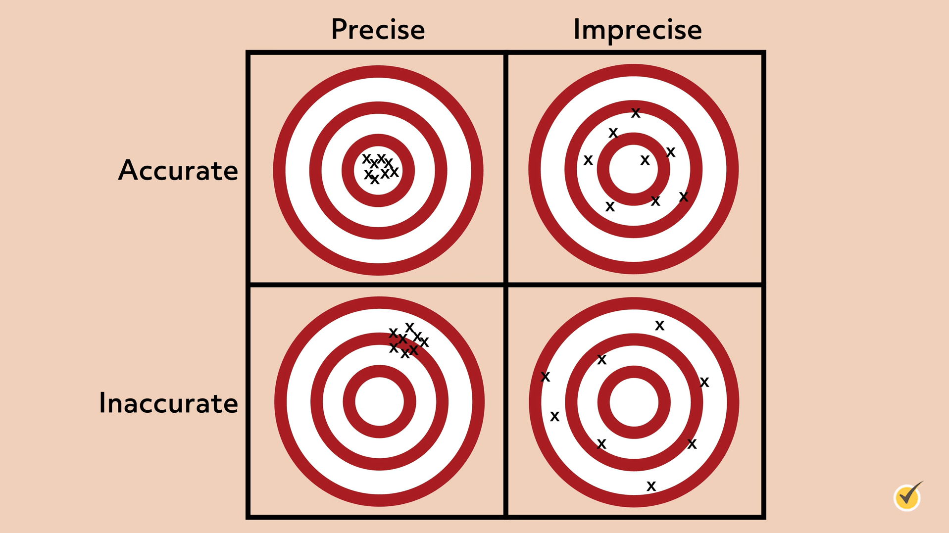
Example 1: Distinguishing between the Accuracy and the Precision of a Set of Values
The diagram shows a target board and four sets of hits on it, A, B, C, and D. The shots were all aimed at the bull’s-eye of the target.

- Which set of hits is both accurate and precise?
- Which set of hits is neither accurate nor precise?
- Which set of hits is accurate but not precise?
- Which set of hits is precise but not accurate?
Answer
We can determine the accuracy of a set of hits by how far from the bull’s-eye the hits are. This can either be for each individual hit in a set or for the average of all the hits in a set.
We can see immediately that for sets B and D, all the hits are either in the blue or white rings, so not close to the bull’s-eye. These hits are not accurate and so sets B and D are not accurate.
We can see immediately that for set A all the hits are close to the bull’s-eye. Set A is accurate.
For set C, two out of three hits are in the red ring and the other hit is in the blue ring. The hits in set C are less accurate than those in set A but more accurate than those in sets B and D. Also, we can consider the average of the hits in set C by taking the point that is equidistant from all the hits in set C, as shown in the following figure.

We can see that the point corresponding to the average of the hits in set C is over the bull’s-eye. We can say that the accuracy of set C is closer to that of set A than of set B or D, and so we call set C accurate.
We can determine the precision of a set of hits by how close the hits are to each other. The sets where the hits are close to each other are sets A and B. In sets C and D, the hits are further from each other.
We can summarize what we have deduced in a table.
| Set | Accuracy | Precision |
|---|---|---|
| (A) | High | High |
| (B) | Low | High |
| (C) | High | Low |
| (D) | Low | Low |
We see then that
- the set that is both accurate and precise is set A,
- the set that is neither accurate nor precise is set D,
- the set that is accurate but not precise is set C,
- the set that is precise but not accurate is set B.
Now let us look at an example in which the effect on accuracy and precision of measurements errors is considered.
Example 2: Distinguishing between the Effect of Systematic Errors on Accuracy and Precision of Measurements
Which of the following statements most correctly describes how systematic measurement errors affect the accuracy and the precision of measurements?
- Systematic errors decrease measurement accuracy.
- Systematic errors decrease both the accuracy and the precision of measurements.
- Systematic errors decrease measurement precision.
- Systematic errors do not affect measurement accuracy or measurement precision.
Answer
In answering this question, we will assume that we are only considering the simplest type of systematic error, for which the error value of a measurement is changed by the same amount for all measurements made.
We can use the analogy of aiming at a target for making a measurement, where the closer to the center of the target a hit is, the more accurate the measurement is. The following figure shows three hits on a target that represent measurements.

An error in a measurement is represented by an increase in the distance between the center of the target and a hit. For systematic errors, the error value is the same for each measurement. This is represented by the hits all moving the same distance in the same direction, as shown in the following figure.

The effect of the systematic error on the hits is to move all the hits away from the center of the target. The accuracy of the measurements represented by the hits is now worse, so we can say that a systematic error decreases measurement accuracy.
We can compare the positions of the hits with and without the systematic error, as shown in the following figure.

We can see that the same triangle that connects the three hits without the error connects the hits with the error. This tells us that the distances of the hits from each other have not been changed by the systematic error. We can say then that a systematic error does not change the precision of a set of measurements.
The correct option is then that systematic errors decrease measurement accuracy.
Now let us look at a similar example.
Example 3: Distinguishing between the Effect of Random Errors on Accuracy and Precision of Measurements
Which of the following statements most correctly describes how random measurement errors affect the accuracy and the precision of measurements?
- Random errors decrease both the accuracy and the precision of measurements.
- Random errors decrease measurement accuracy.
- Random errors decrease measurement precision.
- Random errors do not affect measurement accuracy or measurement precision.
Answer
We can use the analogy of aiming at a target for making a measurement, where the closer to the center of the target a hit is, the more accurate the measurement is. The following figure shows three hits on a target that represent measurements.

An error in a measurement is represented by an increase in the distance between the center of the target and a hit. For random errors, the error value is different for each measurement. This is represented by the hits all moving different distances in different directions, as shown in the following figure.

The effect of the random error on the hits is to move all the hits away from the center of the target. The accuracy of the measurements represented by the hits is now worse, so we can say that a random error decreases measurement accuracy.
We can compare the positions of the hits with and without the random error, as shown in the following figure.

We can see that the triangle that connects the three hits without the error is very different to the triangle that connects the hits with the error. This tells us that the distances of the hits from each other have been changed by the random error. We can say then that a systematic error changes the precision of a set of measurements.
The correct option is then that random errors decrease both the accuracy and the precision of measurements.
Let us now look at an example that explains the usefulness of repeated measurements.
Example 4: Identifying the Usefulness of Repeated Measurements
When taking any measurement, why is it recommended to take the measurement several times and then calculate the average of the readings?
- To reduce the effect of the errors in the individual readings
- Because the average of the readings is the real value of the measurement
- To eliminate any measurement errors in the individual readings
- To increase the precision of the measurement
Answer
Suppose that a measurement is made. It is possible that the measured value includes a random error that produces an error value. The size of the error value is not known.
Suppose instead that the same measurement is repeated many times.
We can use the analogy of aiming at a target for making a measurement, where the closer to the center of the target a hit is, the more accurate the measurement is.
If many measurements are made, the effect of the random error makes each measured value different. This is represented in the following figure.

This representation shows which hits are nearer the bull’s-eye and so makes it seem obvious which measured values are closer to the true value. What is misleading about this representation is that the true value of what is measured is not known, so the same hits could just as plausibly be spread around the target, as shown in the following figure.

We must therefore consider each measurement as equally possibly having the same value as the true value.
If we assume that each measurement is equally likely to give the true value, the following figure shows the distance from each hit to the true value (which we recall is not known).

The following figure shows the errors first as distances from the bull’s-eye and then below that as a set of arrows that all start at different points. In both cases the same set of arrows is shown.

Each of these arrows is equivalent to a vertical and a horizontal arrow, as shown in the following figure.

We can consider just these vertical and horizontal arrows.

These arrows can be separated into vertical arrows and horizontal arrows that point either up, down, left, or right. These arrows can be laid head to tail.

The average length of the arrows pointing up, down, left, and right can be found. This is shown in the following figure.

The horizontal and vertical average arrows can be added together, where the length of a downward arrow is subtracted from the length of an upward arrow, and the length of a leftward arrow is subtracted from the length of a rightward arrow. This gives very small horizontal and vertical lengths, shown in purple.

The purple lines are equivalent to one arrow that points in one direction and has one length.

The resultant arrow is very short. This arrow can now be drawn with its tail at the bull’s-eye. The distance of the head of the arrow from the bull’s-eye represents the error that results from averaging all the measurements made.

We can see that the error due to averaging all the measurements is very small, far smaller than the error of even the measurement that was closest to the true value.
It is important to notice that the average of all the measurements is not exactly equal to the true value. A small error value exists for the average, but this error value is much smaller than the error value for any single measurement.
The option that most closely describes this is that averaging repeated readings is done to reduce the effect of the errors in the individual readings.
Let us now summarize what has been learned in this explainer.
Key Points
- The error value for a measurement is the difference between the measured value and the true value.
- The less the error value of a measurement, the greater the accuracy of the measurement.
- Measurement errors include random errors, systematic errors, and zero errors.
- Random errors change the measured values differently for each measurement made.
- Systematic errors change different measured values equally.
- A nonzero measured value for a true value that is zero is a zero error.
- Precision applies to a set of measurements.
- The smaller the differences of the values of a set of measured values, the more precise the measurements.
- Taking the average of repeated measurements of the same thing can greatly reduce inaccuracy due to random error.
From Wikipedia, the free encyclopedia
Accuracy and precision are two measures of observational error.
Accuracy is how close a given set of measurements (observations or readings) are to their true value, while precision is how close the measurements are to each other.
In other words, precision is a description of random errors, a measure of statistical variability. Accuracy has two definitions:
- More commonly, it is a description of only systematic errors, a measure of statistical bias of a given measure of central tendency; low accuracy causes a difference between a result and a true value; ISO calls this trueness.
- Alternatively, ISO defines[1] accuracy as describing a combination of both types of observational error (random and systematic), so high accuracy requires both high precision and high trueness.
In the first, more common definition of «accuracy» above, the concept is independent of «precision», so a particular set of data can be said to be accurate, precise, both, or neither.
In simpler terms, given a statistical sample or set of data points from repeated measurements of the same quantity, the sample or set can be said to be accurate if their average is close to the true value of the quantity being measured, while the set can be said to be precise if their standard deviation is relatively small.
Common technical definition[edit]

Accuracy is the proximity of measurement results to the accepted value; precision is the degree to which repeated (or reproducible) measurements under unchanged conditions show the same results.
In the fields of science and engineering, the accuracy of a measurement system is the degree of closeness of measurements of a quantity to that quantity’s true value.[2] The precision of a measurement system, related to reproducibility and repeatability, is the degree to which repeated measurements under unchanged conditions show the same results.[2][3] Although the two words precision and accuracy can be synonymous in colloquial use, they are deliberately contrasted in the context of the scientific method.
The field of statistics, where the interpretation of measurements plays a central role, prefers to use the terms bias and variability instead of accuracy and precision: bias is the amount of inaccuracy and variability is the amount of imprecision.
A measurement system can be accurate but not precise, precise but not accurate, neither, or both. For example, if an experiment contains a systematic error, then increasing the sample size generally increases precision but does not improve accuracy. The result would be a consistent yet inaccurate string of results from the flawed experiment. Eliminating the systematic error improves accuracy but does not change precision.
A measurement system is considered valid if it is both accurate and precise. Related terms include bias (non-random or directed effects caused by a factor or factors unrelated to the independent variable) and error (random variability).
The terminology is also applied to indirect measurements—that is, values obtained by a computational procedure from observed data.
In addition to accuracy and precision, measurements may also have a measurement resolution, which is the smallest change in the underlying physical quantity that produces a response in the measurement.
In numerical analysis, accuracy is also the nearness of a calculation to the true value; while precision is the resolution of the representation, typically defined by the number of decimal or binary digits.
In military terms, accuracy refers primarily to the accuracy of fire (justesse de tir), the precision of fire expressed by the closeness of a grouping of shots at and around the centre of the target.[4]
Quantification[edit]
In industrial instrumentation, accuracy is the measurement tolerance, or transmission of the instrument and defines the limits of the errors made when the instrument is used in normal operating conditions.[5]
Ideally a measurement device is both accurate and precise, with measurements all close to and tightly clustered around the true value. The accuracy and precision of a measurement process is usually established by repeatedly measuring some traceable reference standard. Such standards are defined in the International System of Units (abbreviated SI from French: Système international d’unités) and maintained by national standards organizations such as the National Institute of Standards and Technology in the United States.
This also applies when measurements are repeated and averaged. In that case, the term standard error is properly applied: the precision of the average is equal to the known standard deviation of the process divided by the square root of the number of measurements averaged. Further, the central limit theorem shows that the probability distribution of the averaged measurements will be closer to a normal distribution than that of individual measurements.
With regard to accuracy we can distinguish:
- the difference between the mean of the measurements and the reference value, the bias. Establishing and correcting for bias is necessary for calibration.
- the combined effect of that and precision.
A common convention in science and engineering is to express accuracy and/or precision implicitly by means of significant figures. Where not explicitly stated, the margin of error is understood to be one-half the value of the last significant place. For instance, a recording of 843.6 m, or 843.0 m, or 800.0 m would imply a margin of 0.05 m (the last significant place is the tenths place), while a recording of 843 m would imply a margin of error of 0.5 m (the last significant digits are the units).
A reading of 8,000 m, with trailing zeros and no decimal point, is ambiguous; the trailing zeros may or may not be intended as significant figures. To avoid this ambiguity, the number could be represented in scientific notation: 8.0 × 10³ m indicates that the first zero is significant (hence a margin of 50 m) while 8.000 × 10³ m indicates that all three zeros are significant, giving a margin of 0.5 m. Similarly, one can use a multiple of the basic measurement unit: 8.0 km is equivalent to 8.0 × 10³ m. It indicates a margin of 0.05 km (50 m). However, reliance on this convention can lead to false precision errors when accepting data from sources that do not obey it. For example, a source reporting a number like 153,753 with precision +/- 5,000 looks like it has precision +/- 0.5. Under the convention it would have been rounded to 154,000.
Alternatively, in a scientific context, if it is desired to indicate the margin of error with more precision, one can use a notation such as 7.54398(23) × 10−10 m, meaning a range of between 7.54375 and 7.54421 × 10⁻¹⁰ m.
Precision includes:
- repeatability — the variation arising when all efforts are made to keep conditions constant by using the same instrument and operator, and repeating during a short time period; and
- reproducibility — the variation arising using the same measurement process among different instruments and operators, and over longer time periods.
In engineering, precision is often taken as three times Standard Deviation of measurements taken, representing the range that 99.73% of measurements can occur within.[6] For example, an ergonomist measuring the human body can be confident that 99.73% of their extracted measurements fall within ± 0.7 cm — if using the GRYPHON processing system — or ± 13 cm — if using unprocessed data.[7]
ISO definition (ISO 5725)[edit]

According to ISO 5725-1, accuracy consists of trueness (proximity of measurement results to the true value) and precision (repeatability or reproducibility of the measurement).
A shift in the meaning of these terms appeared with the publication of the ISO 5725 series of standards in 1994, which is also reflected in the 2008 issue of the «BIPM International Vocabulary of Metrology» (VIM), items 2.13 and 2.14.[2]
According to ISO 5725-1,[1] the general term «accuracy» is used to describe the closeness of a measurement to the true value. When the term is applied to sets of measurements of the same measurand, it involves a component of random error and a component of systematic error. In this case trueness is the closeness of the mean of a set of measurement results to the actual (true) value and precision is the closeness of agreement among a set of results.
ISO 5725-1 and VIM also avoid the use of the term «bias», previously specified in BS 5497-1,[8] because it has different connotations outside the fields of science and engineering, as in medicine and law.
-

Low accuracy due to low precision
-
Low accuracy even with high precision


In classification[edit]
In binary classification[edit]
Accuracy is also used as a statistical measure of how well a binary classification test correctly identifies or excludes a condition. That is, the accuracy is the proportion of correct predictions (both true positives and true negatives) among the total number of cases examined.[9] As such, it compares estimates of pre- and post-test probability. To make the context clear by the semantics, it is often referred to as the «Rand accuracy» or «Rand index».[10][11][12] It is a parameter of the test.
The formula for quantifying binary accuracy is:

where TP = True positive; FP = False positive; TN = True negative; FN = False negative
Note that, in this context, the concepts of trueness and precision as defined by ISO 5725-1 are not applicable. One reason is that there is not a single “true value” of a quantity, but rather two possible true values for every case, while accuracy is an average across all cases and therefore takes into account both values. However, the term precision is used in this context to mean a different metric originating from the field of information retrieval (see below).
In multiclass classification[edit]
When computing accuracy in multiclass classification, accuracy is simply the fraction of correct classifications:[13]

This is usually expressed as a percentage. For example, if a classifier makes ten predictions and nine of them are correct, the accuracy is 90%.
Accuracy is also called top-1 accuracy to distinguish it from top-5 accuracy, common in convolutional neural network evaluation. To evaluate top-5 accuracy, the classifier must provide relative likelihoods for each class. When these are sorted, a classification is considered correct if the correct classification falls anywhere within the top 5 predictions made by the network. Top-5 accuracy was popularized by the ImageNet challenge. It is usually higher than top-1 accuracy, as any correct predictions in the 2nd through 5th positions will not improve the top-1 score, but do improve the top-5 score.
In psychometrics and psychophysics[edit]
In psychometrics and psychophysics, the term accuracy is interchangeably used with validity and constant error. Precision is a synonym for reliability and variable error. The validity of a measurement instrument or psychological test is established through experiment or correlation with behavior. Reliability is established with a variety of statistical techniques, classically through an internal consistency test like Cronbach’s alpha to ensure sets of related questions have related responses, and then comparison of those related question between reference and target population.[citation needed]
In logic simulation[edit]
In logic simulation, a common mistake in evaluation of accurate models is to compare a logic simulation model to a transistor circuit simulation model. This is a comparison of differences in precision, not accuracy. Precision is measured with respect to detail and accuracy is measured with respect to reality.[14][15]
In information systems[edit]
Information retrieval systems, such as databases and web search engines, are evaluated by many different metrics, some of which are derived from the confusion matrix, which divides results into true positives (documents correctly retrieved), true negatives (documents correctly not retrieved), false positives (documents incorrectly retrieved), and false negatives (documents incorrectly not retrieved). Commonly used metrics include the notions of precision and recall. In this context, precision is defined as the fraction of retrieved documents which are relevant to the query (true positives divided by true+false positives), using a set of ground truth relevant results selected by humans. Recall is defined as the fraction of relevant documents retrieved compared to the total number of relevant documents (true positives divided by true positives+false negatives). Less commonly, the metric of accuracy is used, is defined as the total number of correct classifications (true positives plus true negatives) divided by the total number of documents.
None of these metrics take into account the ranking of results. Ranking is very important for web search engines because readers seldom go past the first page of results, and there are too many documents on the web to manually classify all of them as to whether they should be included or excluded from a given search. Adding a cutoff at a particular number of results takes ranking into account to some degree. The measure precision at k, for example, is a measure of precision looking only at the top ten (k=10) search results. More sophisticated metrics, such as discounted cumulative gain, take into account each individual ranking, and are more commonly used where this is important.
In cognitive systems[edit]
In cognitive systems, accuracy and precision is used to characterize and measure results of a cognitive process performed by biological or artificial entities where a cognitive process is a transformation of data, information, knowledge, or wisdom to a higher-valued form. (DIKW Pyramid) Sometimes, a cognitive process produces exactly the intended or desired output but sometimes produces output far from the intended or desired. Furthermore, repetitions of a cognitive process do not always produce the same output. Cognitive accuracy (CA) is the propensity of a cognitive process to produce the intended or desired output. Cognitive precision (CP) is the propensity of a cognitive process to produce only the intended or desired output.[16][17][18] To measure augmented cognition in human/cog ensembles, where one or more humans work collaboratively with one or more cognitive systems (cogs), increases in cognitive accuracy and cognitive precision assist in measuring the degree of cognitive augmentation.
See also[edit]
- Bias-variance tradeoff in statistics and machine learning
- Accepted and experimental value
- Data quality
- Engineering tolerance
- Exactness (disambiguation)
- Experimental uncertainty analysis
- F-score
- Hypothesis tests for accuracy
- Information quality
- Measurement uncertainty
- Precision (statistics)
- Probability
- Random and systematic errors
- Sensitivity and specificity
- Significant figures
- Statistical significance
References[edit]
- ^ a b BS ISO 5725-1: «Accuracy (trueness and precision) of measurement methods and results — Part 1: General principles and definitions.», p.1 (1994)
- ^ a b c JCGM 200:2008 International vocabulary of metrology — Basic and general concepts and associated terms (VIM)
- ^ Taylor, John Robert (1999). An Introduction to Error Analysis: The Study of Uncertainties in Physical Measurements. University Science Books. pp. 128–129. ISBN 0-935702-75-X.
- ^ North Atlantic Treaty Organization, NATO Standardization Agency AAP-6 – Glossary of terms and definitions, p 43.
- ^ Creus, Antonio. Instrumentación Industrial[citation needed]
- ^ Black, J. Temple (21 July 2020). DeGarmo’s materials and processes in manufacturing. ISBN 978-1-119-72329-5. OCLC 1246529321.
- ^ Parker, Christopher J.; Gill, Simeon; Harwood, Adrian; Hayes, Steven G.; Ahmed, Maryam (2021-05-19). «A Method for Increasing 3D Body Scanning’s Precision: Gryphon and Consecutive Scanning». Ergonomics. 65 (1): 39–59. doi:10.1080/00140139.2021.1931473. ISSN 0014-0139. PMID 34006206.
- ^ BS 5497-1: «Precision of test methods. Guide for the determination of repeatability and reproducibility for a standard test method.» (1979)
- ^ Metz, CE (October 1978). «Basic principles of ROC analysis» (PDF). Semin Nucl Med. 8 (4): 283–98. doi:10.1016/s0001-2998(78)80014-2. PMID 112681. Archived (PDF) from the original on 2022-10-09.
- ^ «Archived copy» (PDF). Archived from the original (PDF) on 2015-03-11. Retrieved 2015-08-09.
{{cite web}}: CS1 maint: archived copy as title (link) - ^ Powers, David M. W. (2015). «What the F-measure doesn’t measure». arXiv:1503.06410 [cs.IR].
- ^ David M W Powers. «The Problem with Kappa» (PDF). Anthology.aclweb.org. Archived (PDF) from the original on 2022-10-09. Retrieved 11 December 2017.
- ^ «3.3. Metrics and scoring: quantifying the quality of predictions». scikit-learn. Retrieved 17 May 2022.
- ^ Acken, John M. (1997). «none». Encyclopedia of Computer Science and Technology. 36: 281–306.
- ^ Glasser, Mark; Mathews, Rob; Acken, John M. (June 1990). «1990 Workshop on Logic-Level Modelling for ASICS». SIGDA Newsletter. 20 (1).
- ^ Fulbright, Ron (2020). Democratization of Expertise: How Cognitive Systems Will Revolutionize Your Life (1st ed.). Boca Raton, FL: CRC Press. ISBN 978-0367859459.
- ^ Fulbright, Ron (2019). «Calculating Cognitive Augmentation – A Case Study». Augmented Cognition. Lecture Notes in Computer Science. Lecture Notes in Computer Science. Springer Cham. 11580: 533–545. arXiv:2211.06479. doi:10.1007/978-3-030-22419-6_38. ISBN 978-3-030-22418-9. S2CID 195891648.
- ^ Fulbright, Ron (2018). «On Measuring Cognition and Cognitive Augmentation». Human Interface and the Management of Information. Information in Applications and Services. Lecture Notes in Computer Science. Lecture Notes in Computer Science. Springer Cham. 10905: 494–507. arXiv:2211.06477. doi:10.1007/978-3-319-92046-7_41. ISBN 978-3-319-92045-0. S2CID 51603737.
External links[edit]
- BIPM — Guides in metrology, Guide to the Expression of Uncertainty in Measurement (GUM) and International Vocabulary of Metrology (VIM)
- «Beyond NIST Traceability: What really creates accuracy», Controlled Environments magazine
- Precision and Accuracy with Three Psychophysical Methods
- Appendix D.1: Terminology, Guidelines for Evaluating and Expressing the Uncertainty of NIST Measurement Results
- Accuracy and Precision
- Accuracy vs Precision — a brief video by Matt Parker
- What’s the difference between accuracy and precision? by Matt Anticole at TED-Ed
Understanding Error and Measurement Confidence
Definitions
Accuracy describes how closely a given measurement matches the true value.
Precision describes the ranges of measured values and is closely related to deviation and standard deviation.
Measurement error is the difference between a measured value, derived from the sample, and the true population value. Measurement error is a metric of accuracy and is usually not precisely knowable.
Measurement uncertainty is an interval around that a measured value such that any repetition of the measurement will produce a new result that lies within this interval. Measurement uncertainty is a metric of precision and can be quantified.
A confidence interval is used to quantify measurement uncertainty. Confidence intervals express the percent certainty that the true value lies within a given range of values.
Example:
A measurement of π yields a 95% confidence interval of π = 3.00 ± 0.5. This indicates that the measurement is 95% certain that the true value of π is between 2.5 and 3.5. Taking the true value of π as π=3.14, we would have a measurement error of 0.14.
Sources of Error
Random Errors
As the name suggests, random errors are random. They cannot be predicted but generally represent themselves as fluctuations centered about the mean.
Common Statistical Errors
Statistical Error: Statistical Error is fundamental to counting experiments due to the familiar relationship between standard deviation and mean value:
![]()
Electronic Noise: Electronic noise is present in measurements involving analog electronic measurements. Critically, the noise will be present even if an analog signal is converted to digital prior to displaying the result.
Daily Patient Alignment Errors: In external beam radiotherapy, daily variation in patient positioning is a source of random errors in the delivered dose distribution.
Systematic Errors
Systematic errors are errors which consistently influence a measurement in a given direction. Systematic errors are most commonly either measurement offsets (E.g. a ruler always measures 1mm long) or a multiplication error (E.g. a ruler that measures 1.1 times the true length). Unlike random errors, systematic errors can be accounted for using a calibration factor.
Common Systematic Errors
Measurement Device Errors: Measurement device errors result from incorrect calibration of the device used to take a measurement.
Atmospherically Induced Errors: Atmospherically induced errors are commonly found in radiation measurement applications where the response of the measurement device is dependent upon temperature or pressure.
Patient Simulation Errors: In external beam radiotherapy, errors in patient or organ positioning that are present during CT simulation will be propagated as systematic error throughout the entire treatment. For example, a CT image which places a tumor 1mm below the true tumor location would yield a treatment plan which delivers dose consistently 1mm below the true tumor.
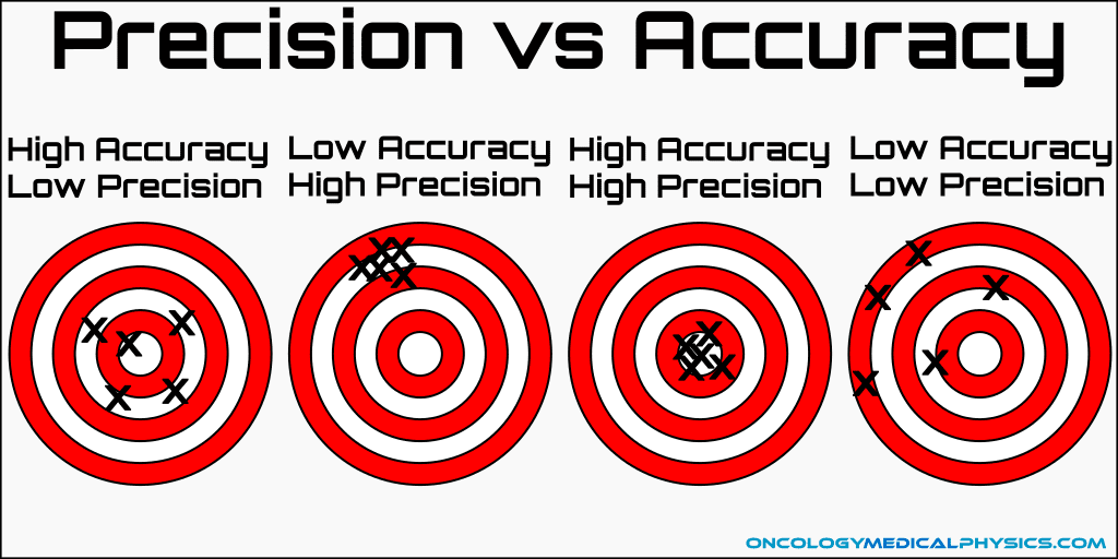
Hello, and welcome to this video about precision, accuracy, and error! Today we’ll learn about the difference between precision and accuracy and when it’s used. We’ll also discuss different types of errors.
Before we get started, let’s review a few things. First, it’s important to remember that many math problems involve measurements of real-world quantities. These measurements include distance, weight, area, volume, temperature, and time. Whenever a quantity is being measured, there is some approximation occurring.
For instance, let’s say you need to measure a length of a wall with a tape measure before hanging a picture frame. To make sure you have the exact length, it’s best to measure the space more than once. When measuring something more than once, it’s possible to have different results. Even though you used the same tool (a tape measure) and are measuring the same space (the wall), differences in measurement can occur.
These differences are called variations, or errors. In this context, the term error does not mean a mistake. Instead, it refers to the difference between a measurement and its actual value, which is also called the known value.
Mathematicians use certain words to talk about differences between a measurement and its known value.
Precision refers to how close repeated measurements are to one another. In other words, it’s how often we get the same result, regardless of if it’s correct or not. If the measurement is consistent, it is considered to be more reliable.
Think of the measurements as points on a target.

The target on the left shows precision because all measurements are approximately the same. The target on the right does not show precision because these measurements are not approximately the same.
Accuracy refers to how close a measurement comes to the true or actual measurement of the object. In other words, it’s used to describe how close the data is to the correct data.
Consider these two targets:

Assuming that the true or actual measurement is the target’s bullseye, the target on the left shows accuracy and precision. All measurements are located at the bullseye. The target on the right does not show accuracy, even though it is precise, because the measurements are not located at or near the bullseye.
Since accuracy and precision mean two different things, measurements can be both accurate and precise. Measuring systems are considered valid if they are both accurate and precise. On the other hand, measurements can be precise without being accurate, and they can be accurate without being precise. Consider these targets:
As you can see, the upper left target shows measurements that are accurate and precise. All measurements are consistent and at the bullseye. In the upper-right target, we can see measurements that are accurate but imprecise. These measurements are not consistent but they are all close to the bullseye. In the lower-left target, the measurements are precise but inaccurate. Although they’re consistent, the measurements are not near the bullseye. Finally, in the lower right target, the measurements are neither precise nor accurate. They are inconsistent and not near the bullseye.
Now that we’ve covered accuracy and precision, let’s talk about errors.
Approximate error refers to the amount of error in a physical measurement. Approximate error is often reported as the measurement, followed by the plus or minus sign ((pm )) and the amount of the approximate error. For instance, consider an approximate error of (6.8pm 0.05) inches. This gives us a range of (6.8-0.05) to (6.8+0.05), which equals 6.75 to 6.85 inches. This range is known as a tolerance interval. It is the range in which measurements are tolerated or considered acceptable.
The greatest possible error (also called the maximum possible error) is calculated by adding or subtracting half of the measuring unit to the measurement. For instance, let’s say you measure the length of a wall to be 90 inches. The unit of measurement is 1 inch, so the greatest possible error is one-half of 1 inch, or 0.5 inches. In other words, any measurements in the range of 89.5 inches to 90.5 inches are considered valid. The tolerance interval is written as (90pm 0.5) inches.
Let’s look at an example of using the greatest possible error together. One gallon of water weighs about 8.3 pounds. What is the greatest possible error and the tolerance interval created by that error?
First, we need to identify the unit of measurement. In this case, the unit of measurement is one-tenth, or 0.1. Therefore, the greatest possible error is one-half of one-tenth, or 0.05, and the tolerance interval would be (8.3pm 0.05) pounds.
Now it’s your turn.
A furniture delivery box weighs about 22 pounds. What is the greatest possible error and the tolerance interval?
Pause the video and see if you can do this one by yourself. When you’re ready, press play and we’ll go over everything together.
Okay, let’s work through this.
First, we need to identify the unit of measurement, which is 1 pound. The greatest possible error is one-half of the unit of measurement, which is 0.5 pounds. Therefore, the tolerance interval is (22pm 0.5) pounds.
Great job!
Now onto some different methods to show errors in measurement. One of these methods is called absolute error. The absolute error is the absolute value of the difference between a measurement’s measured value and its known value.
(text {Absolute error}=left | text{measured value-known value} right |)
The difference is always reported as a positive number, which is why there are absolute value bars shown in the formula. Let’s look at an example.
Say you know a chemistry experiment will yield 10 milliliters but your solution is 9.5 milliliters. Since (10-9.5=0.5), the absolute error in this scenario is 0.5 milliliters.
When the known value is not known or is not given, then the absolute error is equal to the greatest possible error. For example, in the measurement (18pm 0.5) centimeters, no known value is given. In this case, the absolute error is 0.5 centimeters.
Another way to represent errors in measurement is with relative error. Relative error shows the significance of an error by comparing it to the original measurement. To find the relative error, find the difference between the measured value and the known value, and divide its absolute value by the known value.
(text {Relative error}=frac{left | text{measured value-known value} right |}{text{known value}})
Let’s find the relative error of the chemistry experiment example we just discussed. Recall that the known value was 10 milliliters and the measured value was 9.5 milliliters. To find the relative error, substitute these values into the formula and solve.
Since our measured value is 9.5, and our known value is 10, take the absolute value of (9.5-10) and divide it by 10.
(text {Relative error}=frac{left | text{measured value-known value} right |}{text{known value}})
(=frac{|9.5-10|}{10})
(=frac{|-0.5|}{10})
(=frac{0.5}{10})
(=0.05 text{ milliliters})
If there is no known value given, then the relative error is found by dividing the greatest possible error by the measured value.
(text {Relative error}=frac{text{greatest possible error}}{text{measured value}})
In the measurement (18pm 0.5) centimeters, no known value is given. Recall that in this case, the greatest possible error is 0.5 centimeters. To find the relative error, substitute these values into the formula and solve:
(text {Relative error}=frac{text{greatest possible error}}{text{measured value}}=frac{0.5}{18}approx 0.027text{ centimeters})
Compared to absolute error, relative error is often seen as more useful because absolute error doesn’t show the significance of the error in context. For example, a soccer field is 2,700 inches long and your measurement is off by 0.5 inches, 2,699.5 inches. In this case, that 0.5 inches won’t throw off your calculations too much. However, if a post-it note is 3 inches long and your measured value is off by the same 0.5 inches, and you get 2.5 inches, that’s a much more significant difference due to the size of the post-it note.
In our relative error formula, dividing by the known value gives us that context of if our object is off by 0.5 inches compared to a really large number like with our soccer field, or off by 0.5 inches compared to a really small number like with our post-it note. Absolute error only tells us that we are off by 0.5 inches.
A third way to represent errors in measurement is by calculating the percent of error. To find the percent of error, multiply the relative error by 100 to make it a percent.
In the chemistry example, we found that the relative error was 0.05 milliliters. 0.05 times 100 equals 5, so the percent of error in this experiment is 5%.
Now that we know how to show different errors in measurement, let’s take a look at an example together.
Consider a bedroom with a known length of 16 feet. The bedroom is measured to be 16.5 feet long. Let’s find the absolute error, relative error, and percent of error.
(text{Absolute error}=left | text{measured value-known value} right |)
(=left | 16.5-16 right |)
(=0.5text{ feet})
(text{Relative error}=frac{left | text{measured value-known value} right |}{text {known value}})
(=frac{left | 16.5-16 right |}{16})
(=frac{0.5}{16})
(=0.03125)
(0.03125times 100=3.125%)
Therefore, the difference in measurement of the bedroom was 0.5 feet, which is just over a 3% error.
Let’s take a look at another example. Consider the measurement of (2.5pm 0.5) inches. Unlike our last example, there is no known value given.
(text{Relative error}=frac{text{greatest possible error}}{text{measured value}}=frac{0.5}{2.5}=0.2text{ inches})
(0.2times 100=20%)
Therefore, the 0.5-inch difference in measurement is a 20% error.
Now it’s your turn. I’m going to give you a set of measurements, and you’re going to find the absolute error, relative error, and percent of error. This one is a little more challenging, but I know you can do it.
Micah is using a ruler to find the radius of a circle. He measures the radius to be 5.5 centimeters, but the actual length of the radius is 5.8 centimeters. Find Micah’s absolute error, relative error, and percent of error.
Pause the video and see if you can do this one by yourself. When you’re ready, press play and we’ll go over it together.
Now that you’ve tried this problem by yourself, let’s go over it together.
(text{Absolute error}=left | text{measured value-known value} right |)
(=left | 5.5-5.8 right |)
(=left | -0.3 right |)
(=0.3text{ centimeters})
(text{Relative error}=frac{left | text{measured value-known value} right |}{text{known value}})
(=frac{left | 5.5-5.8 right |}{5.8})
(=frac{0.3}{5.8})
(=0.05172414 text{ centimeters})
(0.05172414times 100=5.17241379% approx 5.17%)
Therefore, the difference in measurement of the circle is 0.3 centimeters, which is just over a 5% error.
I hope this video about precision, accuracy, and error was helpful. Thanks for watching, and happy studying!
Practice Questions
Question #1:
Five darts are thrown at a target aiming for the target’s bullseye (the target’s center). All five darts hit the target. The letter (x) indicates where a dart hits the target. Which of the following targets best shows that the five throws were accurate but imprecise?
Show Answer
Answer:
Darts thrown closest to the bullseye are considered accurate throws, but they do not necessarily have to be close to each other. Choices C and D are considered accurate compared to choices A and B since all five darts thrown are closer to the bullseye. Imprecise dart throws do not land close to each other on the target (but they may still be considered accurate throws). Consider the two accurate throws between choices C and D. The darts thrown on the target for choice C are considered imprecise since they are not as close to each other as the darts in choice D. Therefore, choice C is the best answer choice showing the five throws were accurate but imprecise.
Hide Answer
Question #2:
One liter of water weighs approximately 2.2 pounds. What is the tolerance interval created by the greatest possible error when a liter of water is weighed?
(2.2pm0.05text{ pounds})
(2.2pm0.5text{ pounds})
(2.2pm0.01text{ pounds})
(2.2pm0.1text{ pounds})
Show Answer
Answer:
The greatest possible error (also called the maximum possible error) is calculated by adding or subtracting one-half of the measuring unit to the measurement. The unit of measurement for our liter of water is measured to the nearest one-tenth of a pound. So, the greatest possible error is one-half of 0.1 pounds, which is 0.05 pounds.
A tolerance interval is the range of values in which measurements are tolerated or considered acceptable. The tolerance interval can be written as the given measurement (pm) the greatest possible error. So, the tolerance interval for the weight of one liter of water is (2.2pm0.05text{ pounds}).
Hide Answer
Question #3:
It is known that the volume of a given cube is (27text{ cm}^3). You measure the length of one of the sides of the cube and calculate its volume to be (24.21text{ cm}^3). What is the relative error in your calculation?
Show Answer
Answer:
The relative error is the ratio of the absolute error and the actual value of a measurement.
The absolute error is the absolute value of the difference between a measurement’s measured value and its known value.
(text{Absolute error}=left|text{measured value}-text{known value}right|)
So, the relative error is:
(text{Relative error}=frac{left|text{measured value}-text{known value}right|}{text{known value}})
The known value for the volume of the cube is (27text{ cm}^3) and the measured value is (29.79text{ cm}^3). So, the absolute error is (left|24.21text{ cm}^3-27text{ cm}^3right|=left|-2.79text{ cm}^3right|=2.79text{ cm}^3). Then, the relative error is:
(text{Relative error}=frac{2.79}{27}approx0.103)
Hide Answer
Question #4:
You measure the length and width of a rectangular picture frame with a metric ruler. You then calculate the area using your measurements to be (25,402.58text{ cm}^3). What is the greatest possible error and the tolerance interval created by that error in centimeters?
(0.0005text{ cm});(25{,}402.58pm0.0005text{ cm})
(0.005text{ cm});(25{,}402.58pm0.005text{ cm})
(0.05text{ cm});(25{,}402.58pm0.05text{ cm})
(0.5text{ cm});(25{,}402.58pm0.5text{ cm})
Show Answer
Answer:
The greatest possible error (also called the maximum possible error) is calculated by finding one-half of the measuring unit to the measurement. The unit of measurement for our calculated area of the picture frame is to the nearest hundredth of a square centimeter, so the greatest possible error is one-half of 0.01 cm, which is 0.005 cm.
A tolerance interval is the range of values in which measurements are tolerated or considered acceptable. The tolerance interval can be written as the calculated measurement (pm) the greatest possible error. So, the tolerance interval for the measured area of our picture frame is (25{,}402.58pm0.005text{ cm}).
Hide Answer
Question #5:
You are making some cookies from scratch. The recipe for the cookie batter calls for one cup (8 ounces) of water. You put 8.2 ounces of water into the cookie batter. What is the percent of error of your measurement?
Show Answer
Answer:
First find the relative error, then multiply its value by 100 to convert it to a percent of error.
The relative error is the ratio of the absolute error and the actual value of a measurement. The absolute error is the absolute value of the difference between a measurement’s measured value and its known value.
(text{Absolute error}=left|text{measured value}-text{known value}right|)
So, the relative error is:
(text{Relative error}=frac{left|text{measured value}-text{known value}right|}{text{known value}})
The known value for a cup of water is 8 ounces, and the measured value is 8.2 ounces. So, the absolute error is (left|8.2text{ oz}-8text{ oz}right|=0.2text{ oz}). Then, the relative error is:
(text{Relative error}=frac{0.2}{8}=0.025)
So, the percent of error is (0.025times100=2.5%).
Hide Answer