Есть 3 различных API для оценки качества прогнозов модели:
- Метод оценки оценщика : у оценщиков есть
scoreметод, обеспечивающий критерий оценки по умолчанию для проблемы, для решения которой они предназначены. Это обсуждается не на этой странице, а в документации каждого оценщика. - Параметр оценки: инструменты оценки модели с использованием перекрестной проверки (например,
model_selection.cross_val_scoreиmodel_selection.GridSearchCV) полагаются на внутреннюю стратегию оценки . Это обсуждается в разделе Параметр оценки: определение правил оценки модели . - Метрические функции : В
sklearn.metricsмодуле реализованы функции оценки ошибки прогноза для конкретных целей. Эти показатели подробно описаны в разделах по метрикам классификации , MultiLabel ранжирования показателей , показателей регрессии и показателей кластеризации .
Наконец, фиктивные оценки полезны для получения базового значения этих показателей для случайных прогнозов.
3.3.1. В scoring параметрах: определение правил оценки моделей
Выбор и оценка модели с использованием таких инструментов, как model_selection.GridSearchCV и model_selection.cross_val_score, принимают scoring параметр, который контролирует, какую метрику они применяют к оцениваемым оценщикам.
3.3.1.1. Общие случаи: предопределенные значения
Для наиболее распространенных случаев использования вы можете назначить объект подсчета с помощью scoring параметра; в таблице ниже показаны все возможные значения. Все объекты счетчика следуют соглашению о том, что более высокие возвращаемые значения лучше, чем более низкие возвращаемые значения . Таким образом, метрики, которые измеряют расстояние между моделью и данными, например metrics.mean_squared_error, доступны как neg_mean_squared_error, которые возвращают инвертированное значение метрики.
| Подсчет очков | Функция | Комментарий |
| Классификация | ||
| ‘accuracy’ | metrics.accuracy_score |
|
| ‘balanced_accuracy’ | metrics.balanced_accuracy_score |
|
| ‘top_k_accuracy’ | metrics.top_k_accuracy_score |
|
| ‘average_precision’ | metrics.average_precision_score |
|
| ‘neg_brier_score’ | metrics.brier_score_loss |
|
| ‘f1’ | metrics.f1_score |
для двоичных целей |
| ‘f1_micro’ | metrics.f1_score |
микро-усредненный |
| ‘f1_macro’ | metrics.f1_score |
микро-усредненный |
| ‘f1_weighted’ | metrics.f1_score |
средневзвешенное |
| ‘f1_samples’ | metrics.f1_score |
по многопозиционному образцу |
| ‘neg_log_loss’ | metrics.log_loss |
требуетсяpredict_probaподдержка |
| ‘precision’ etc. | metrics.precision_score |
суффиксы применяются как с ‘f1’ |
| ‘recall’ etc. | metrics.recall_score |
суффиксы применяются как с ‘f1’ |
| ‘jaccard’ etc. | metrics.jaccard_score |
суффиксы применяются как с ‘f1’ |
| ‘roc_auc’ | metrics.roc_auc_score |
|
| ‘roc_auc_ovr’ | metrics.roc_auc_score |
|
| ‘roc_auc_ovo’ | metrics.roc_auc_score |
|
| ‘roc_auc_ovr_weighted’ | metrics.roc_auc_score |
|
| ‘roc_auc_ovo_weighted’ | metrics.roc_auc_score |
|
| Кластеризация | ||
| ‘adjusted_mutual_info_score’ | metrics.adjusted_mutual_info_score |
|
| ‘adjusted_rand_score’ | metrics.adjusted_rand_score |
|
| ‘completeness_score’ | metrics.completeness_score |
|
| ‘fowlkes_mallows_score’ | metrics.fowlkes_mallows_score |
|
| ‘homogeneity_score’ | metrics.homogeneity_score |
|
| ‘mutual_info_score’ | metrics.mutual_info_score |
|
| ‘normalized_mutual_info_score’ | metrics.normalized_mutual_info_score |
|
| ‘rand_score’ | metrics.rand_score |
|
| ‘v_measure_score’ | metrics.v_measure_score |
|
| Регрессия | ||
| ‘explained_variance’ | metrics.explained_variance_score |
|
| ‘max_error’ | metrics.max_error |
|
| ‘neg_mean_absolute_error’ | metrics.mean_absolute_error |
|
| ‘neg_mean_squared_error’ | metrics.mean_squared_error |
|
| ‘neg_root_mean_squared_error’ | metrics.mean_squared_error |
|
| ‘neg_mean_squared_log_error’ | metrics.mean_squared_log_error |
|
| ‘neg_median_absolute_error’ | metrics.median_absolute_error |
|
| ‘r2’ | metrics.r2_score |
|
| ‘neg_mean_poisson_deviance’ | metrics.mean_poisson_deviance |
|
| ‘neg_mean_gamma_deviance’ | metrics.mean_gamma_deviance |
|
| ‘neg_mean_absolute_percentage_error’ | metrics.mean_absolute_percentage_error |
Примеры использования:
>>> from sklearn import svm, datasets
>>> from sklearn.model_selection import cross_val_score
>>> X, y = datasets.load_iris(return_X_y=True)
>>> clf = svm.SVC(random_state=0)
>>> cross_val_score(clf, X, y, cv=5, scoring='recall_macro')
array([0.96..., 0.96..., 0.96..., 0.93..., 1.        ])
>>> model = svm.SVC()
>>> cross_val_score(model, X, y, cv=5, scoring='wrong_choice')
Traceback (most recent call last):
ValueError: 'wrong_choice' is not a valid scoring value. Use sorted(sklearn.metrics.SCORERS.keys()) to get valid options.
Примечание
Значения, перечисленные в виде ValueError исключения, соответствуют функциям измерения точности прогнозирования, описанным в следующих разделах. Объекты счетчика для этих функций хранятся в словаре sklearn.metrics.SCORERS.
3.3.1.2. Определение стратегии выигрыша от метрических функций
Модуль sklearn.metrics также предоставляет набор простых функций, измеряющих ошибку предсказания с учетом истинности и предсказания:
- функции, заканчивающиеся на,
_scoreвозвращают значение для максимизации, чем выше, тем лучше. - функции, заканчивающиеся на
_errorили_lossвозвращающие значение, которое нужно минимизировать, чем ниже, тем лучше. При преобразовании в объект счетчика с использованиемmake_scorerустановите дляgreater_is_betterпараметра значениеFalse(Trueпо умолчанию; см. Описание параметра ниже).
Метрики, доступные для различных задач машинного обучения, подробно описаны в разделах ниже.
Многим метрикам не даются имена для использования в качестве scoring значений, иногда потому, что они требуют дополнительных параметров, например fbeta_score. В таких случаях вам необходимо создать соответствующий объект оценки. Самый простой способ создать вызываемый объект для оценки — использовать make_scorer. Эта функция преобразует метрики в вызываемые объекты, которые можно использовать для оценки модели.
Один из типичных вариантов использования — обернуть существующую метрическую функцию из библиотеки значениями, отличными от значений по умолчанию для ее параметров, такими как beta параметр для fbeta_score функции:
>>> from sklearn.metrics import fbeta_score, make_scorer
>>> ftwo_scorer = make_scorer(fbeta_score, beta=2)
>>> from sklearn.model_selection import GridSearchCV
>>> from sklearn.svm import LinearSVC
>>> grid = GridSearchCV(LinearSVC(), param_grid={'C': [1, 10]},
...                     scoring=ftwo_scorer, cv=5)
Второй вариант использования — создание полностью настраиваемого объекта скоринга из простой функции Python с использованием make_scorer, которая может принимать несколько параметров:
- функция Python, которую вы хотите использовать (
my_custom_loss_funcв примере ниже) - возвращает ли функция Python оценку (
greater_is_better=True, по умолчанию) или потерю (greater_is_better=False). В случае потери результат функции python аннулируется объектом скоринга в соответствии с соглашением о перекрестной проверке, согласно которому скоринтеры возвращают более высокие значения для лучших моделей. - только для показателей классификации: требуется ли для предоставленной вами функции Python постоянная уверенность в принятии решений (
needs_threshold=True). Значение по умолчанию неверно. - любые дополнительные параметры, такие как
betaилиlabelsвf1_score.
Вот пример создания пользовательских счетчиков очков и использования greater_is_better параметра:
>>> import numpy as np
>>> def my_custom_loss_func(y_true, y_pred):
...     diff = np.abs(y_true - y_pred).max()
...     return np.log1p(diff)
...
>>> # score will negate the return value of my_custom_loss_func,
>>> # which will be np.log(2), 0.693, given the values for X
>>> # and y defined below.
>>> score = make_scorer(my_custom_loss_func, greater_is_better=False)
>>> X = [[1], [1]]
>>> y = [0, 1]
>>> from sklearn.dummy import DummyClassifier
>>> clf = DummyClassifier(strategy='most_frequent', random_state=0)
>>> clf = clf.fit(X, y)
>>> my_custom_loss_func(y, clf.predict(X))
0.69...
>>> score(clf, X, y)
-0.69...
3.3.1.3. Реализация собственного скорингового объекта
Вы можете сгенерировать еще более гибкие модели скоринга, создав свой собственный скоринговый объект с нуля, без использования make_scorer фабрики. Чтобы вызываемый может быть бомбардиром, он должен соответствовать протоколу, указанному в следующих двух правилах:
- Его можно вызвать с параметрами (estimator, X, y), где estimator это модель, которая должна быть оценена, X это данные проверки и y основная истинная цель для (в контролируемом случае) или None (в неконтролируемом случае).
- Он возвращает число с плавающей запятой, которое количественно определяет
estimatorкачество прогнозированияXсо ссылкой наy. Опять же, по соглашению более высокие числа лучше, поэтому, если ваш секретарь сообщает о проигрыше, это значение следует отменить.
Примечание Использование пользовательских счетчиков в функциях, где n_jobs> 1
Хотя определение пользовательской функции оценки вместе с вызывающей функцией должно работать из коробки с бэкэндом joblib по умолчанию (loky), его импорт из другого модуля будет более надежным подходом и будет работать независимо от бэкэнда joblib.
Например, чтобы использовать n_jobsбольше 1 в примере ниже, custom_scoring_function функция сохраняется в созданном пользователем модуле ( custom_scorer_module.py) и импортируется:
>>> from custom_scorer_module import custom_scoring_function
>>> cross_val_score(model,
...  X_train,
...  y_train,
...  scoring=make_scorer(custom_scoring_function, greater_is_better=False),
...  cv=5,
...  n_jobs=-1)
3.3.1.4. Использование множественной метрической оценки
Scikit-learn также позволяет оценивать несколько показателей в GridSearchCV, RandomizedSearchCV и cross_validate.
Есть три способа указать несколько показателей оценки для scoring параметра:
- Как итерация строковых показателей:
>>> scoring = ['accuracy', 'precision']
- В качестве
dictсопоставления имени секретаря с функцией подсчета очков:
>>> from sklearn.metrics import accuracy_score
>>> from sklearn.metrics import make_scorer
>>> scoring = {'accuracy': make_scorer(accuracy_score),
...            'prec': 'precision'}
Обратите внимание, что значения dict могут быть либо функциями счетчика, либо одной из предварительно определенных строк показателей.
- Как вызываемый объект, возвращающий словарь оценок:
>>> from sklearn.model_selection import cross_validate
>>> from sklearn.metrics import confusion_matrix
>>> # A sample toy binary classification dataset
>>> X, y = datasets.make_classification(n_classes=2, random_state=0)
>>> svm = LinearSVC(random_state=0)
>>> def confusion_matrix_scorer(clf, X, y):
...      y_pred = clf.predict(X)
...      cm = confusion_matrix(y, y_pred)
...      return {'tn': cm[0, 0], 'fp': cm[0, 1],
...              'fn': cm[1, 0], 'tp': cm[1, 1]}
>>> cv_results = cross_validate(svm, X, y, cv=5,
...                             scoring=confusion_matrix_scorer)
>>> # Getting the test set true positive scores
>>> print(cv_results['test_tp'])
[10  9  8  7  8]
>>> # Getting the test set false negative scores
>>> print(cv_results['test_fn'])
[0 1 2 3 2]
3.3.2. Метрики классификации
В sklearn.metrics модуле реализованы несколько функций потерь, оценки и полезности для измерения эффективности классификации. Некоторые метрики могут потребовать оценок вероятности положительного класса, значений достоверности или значений двоичных решений. Большинство реализаций позволяют каждой выборке вносить взвешенный вклад в общую оценку с помощью sample_weight параметра.
Некоторые из них ограничены случаем двоичной классификации:
precision_recall_curve(y_true, probas_pred, *) |
Вычислите пары точности-отзыва для разных пороговых значений вероятности. |
roc_curve(y_true, y_score, *[, pos_label, …]) |
Вычислить рабочую характеристику приемника (ROC). |
det_curve(y_true, y_score[, pos_label, …]) |
Вычислите частоту ошибок для различных пороговых значений вероятности. |
Другие также работают в случае мультикласса:
balanced_accuracy_score(y_true, y_pred, *[, …]) |
Вычислите сбалансированную точность. |
cohen_kappa_score(y1, y2, *[, labels, …]) |
Каппа Коэна: статистика, измеряющая согласованность аннотаторов. |
confusion_matrix(y_true, y_pred, *[, …]) |
Вычислите матрицу неточностей, чтобы оценить точность классификации. |
hinge_loss(y_true, pred_decision, *[, …]) |
Средняя потеря петель (нерегулируемая). |
matthews_corrcoef(y_true, y_pred, *[, …]) |
Вычислите коэффициент корреляции Мэтьюза (MCC). |
roc_auc_score(y_true, y_score, *[, average, …]) |
Вычислить площадь под кривой рабочих характеристик приемника (ROC AUC) по оценкам прогнозов. |
top_k_accuracy_score(y_true, y_score, *[, …]) |
Top-k Рейтинг по классификации точности. |
Некоторые также работают в многоярусном регистре:
accuracy_score(y_true, y_pred, *[, …]) |
Классификационная оценка точности. |
classification_report(y_true, y_pred, *[, …]) |
Создайте текстовый отчет, показывающий основные показатели классификации. |
f1_score(y_true, y_pred, *[, labels, …]) |
Вычислите оценку F1, также известную как сбалансированная оценка F или F-мера. |
fbeta_score(y_true, y_pred, *, beta[, …]) |
Вычислите оценку F-beta. |
hamming_loss(y_true, y_pred, *[, sample_weight]) |
Вычислите среднюю потерю Хэмминга. |
jaccard_score(y_true, y_pred, *[, labels, …]) |
Оценка коэффициента сходства Жаккара. |
log_loss(y_true, y_pred, *[, eps, …]) |
Потеря журнала, также известная как потеря логистики или потеря кросс-энтропии. |
multilabel_confusion_matrix(y_true, y_pred, *) |
Вычислите матрицу неточностей для каждого класса или образца. |
precision_recall_fscore_support(y_true, …) |
Точность вычислений, отзыв, F-мера и поддержка для каждого класса. |
precision_score(y_true, y_pred, *[, labels, …]) |
Вычислите точность. |
recall_score(y_true, y_pred, *[, labels, …]) |
Вычислите отзыв. |
roc_auc_score(y_true, y_score, *[, average, …]) |
Вычислить площадь под кривой рабочих характеристик приемника (ROC AUC) по оценкам прогнозов. |
zero_one_loss(y_true, y_pred, *[, …]) |
Потеря классификации нулевая единица. |
А некоторые работают с двоичными и многозначными (но не мультиклассовыми) проблемами:
В следующих подразделах мы опишем каждую из этих функций, которым будут предшествовать некоторые примечания по общему API и определению показателей.
3.3.2.1. От бинарного до мультиклассового и многозначного
Некоторые метрики по существу определены для задач двоичной классификации (например f1_score, roc_auc_score). В этих случаях по умолчанию оценивается только положительная метка, предполагая по умолчанию, что положительный класс помечен 1 (хотя это можно настроить с помощью pos_label параметра).
При расширении двоичной метрики на задачи с несколькими классами или метками данные обрабатываются как набор двоичных задач, по одной для каждого класса. Затем есть несколько способов усреднить вычисления двоичных показателей по набору классов, каждый из которых может быть полезен в некотором сценарии. Если возможно, вы должны выбрать одно из них с помощью average параметра.
"macro"просто вычисляет среднее значение двоичных показателей, придавая каждому классу одинаковый вес. В задачах, где редкие занятия тем не менее важны, макро-усреднение может быть средством выделения их производительности. С другой стороны, предположение, что все классы одинаково важны, часто неверно, так что макро-усреднение будет чрезмерно подчеркивать обычно низкую производительность для нечастого класса."weighted"учитывает дисбаланс классов, вычисляя среднее значение двоичных показателей, в которых оценка каждого класса взвешивается по его присутствию в истинной выборке данных."micro"дает каждой паре выборка-класс равный вклад в общую метрику (за исключением результата взвешивания выборки). Вместо того, чтобы суммировать метрику для каждого класса, это суммирует дивиденды и делители, составляющие метрики для каждого класса, для расчета общего частного. Микро-усреднение может быть предпочтительным в настройках с несколькими ярлыками, включая многоклассовую классификацию, когда класс большинства следует игнорировать."samples"применяется только к задачам с несколькими ярлыками. Он не вычисляет меру для каждого класса, вместо этого вычисляет метрику по истинным и прогнозируемым классам для каждой выборки в данных оценки и возвращает их (sample_weight— взвешенное) среднее значение.- Выбор
average=Noneвернет массив с оценкой для каждого класса.
В то время как данные мультикласса предоставляются метрике, как двоичные цели, в виде массива меток классов, данные с несколькими метками указываются как индикаторная матрица, в которой ячейка [i, j] имеет значение 1, если у образца i есть метка j, и значение 0 в противном случае.
3.3.2.2. Оценка точности
Функция accuracy_score вычисляет точность , либо фракции ( по умолчанию) или количество (нормализует = False) правильных предсказаний.
В классификации с несколькими ярлыками функция возвращает точность подмножества. Если весь набор предсказанных меток для выборки строго соответствует истинному набору меток, то точность подмножества равна 1,0; в противном случае — 0, 0.
Если $hat{y}_i$ прогнозируемое значение $i$-й образец и $y_i$ — соответствующее истинное значение, тогда доля правильных прогнозов по сравнению с $n_{samples}$ определяется как
$$texttt{accuracy}(y, hat{y}) = frac{1}{n_text{samples}} sum_{i=0}^{n_text{samples}-1} 1(hat{y}_i = y_i)$$
где $1(x)$- индикаторная функция .
>>> import numpy as np
>>> from sklearn.metrics import accuracy_score
>>> y_pred = [0, 2, 1, 3]
>>> y_true = [0, 1, 2, 3]
>>> accuracy_score(y_true, y_pred)
0.5
>>> accuracy_score(y_true, y_pred, normalize=False)
2
В многопозиционном корпусе с бинарными индикаторами меток:
>>> accuracy_score(np.array([[0, 1], [1, 1]]), np.ones((2, 2)))
0.5
Пример:
- См. В разделе Проверка с перестановками значимости классификационной оценки пример использования показателя точности с использованием перестановок набора данных.
3.3.2.3. Рейтинг точности Top-k
Функция top_k_accuracy_score представляет собой обобщение accuracy_score. Разница в том, что прогноз считается правильным, если истинная метка связана с одним из kнаивысших прогнозируемых баллов. accuracy_score является частным случаем k = 1.
Функция охватывает случаи двоичной и многоклассовой классификации, но не случай многозначной классификации.
Если $hat{f}_{i,j}$ прогнозируемый класс для $i$-й образец, соответствующий $j$-й по величине прогнозируемый результат и $y_i$ — соответствующее истинное значение, тогда доля правильных прогнозов по сравнению с $n_{samples}$ определяется как
$$texttt{top-k accuracy}(y, hat{f}) = frac{1}{n_text{samples}} sum_{i=0}^{n_text{samples}-1} sum_{j=1}^{k} 1(hat{f}_{i,j} = y_i)$$
где k допустимое количество предположений и 1(x)- индикаторная функция.
>>> import numpy as np
>>> from sklearn.metrics import top_k_accuracy_score
>>> y_true = np.array([0, 1, 2, 2])
>>> y_score = np.array([[0.5, 0.2, 0.2],
...                     [0.3, 0.4, 0.2],
...                     [0.2, 0.4, 0.3],
...                     [0.7, 0.2, 0.1]])
>>> top_k_accuracy_score(y_true, y_score, k=2)
0.75
>>> # Not normalizing gives the number of "correctly" classified samples
>>> top_k_accuracy_score(y_true, y_score, k=2, normalize=False)
3
3.3.2.4. Сбалансированный показатель точности
Функция balanced_accuracy_score вычисляет взвешенную точность , что позволяет избежать завышенных оценок производительности на несбалансированных данных. Это макросреднее количество оценок отзыва по классу или, что то же самое, грубая точность, где каждая выборка взвешивается в соответствии с обратной распространенностью ее истинного класса. Таким образом, для сбалансированных наборов данных оценка равна точности.
В двоичном случае сбалансированная точность равна среднему арифметическому чувствительности (истинно положительный показатель) и специфичности (истинно отрицательный показатель) или площади под кривой ROC с двоичными прогнозами, а не баллами:
$$texttt{balanced-accuracy} = frac{1}{2}left( frac{TP}{TP + FN} + frac{TN}{TN + FP}right )$$
Если классификатор одинаково хорошо работает в любом классе, этот термин сокращается до обычной точности (т. е. Количества правильных прогнозов, деленного на общее количество прогнозов).
Напротив, если обычная точность выше вероятности только потому, что классификатор использует несбалансированный набор тестов, тогда сбалансированная точность, при необходимости, упадет до $frac{1}{n_classes}$.
Оценка варьируется от 0 до 1 или, когда adjusted=True используется, масштабируется до диапазона $frac{1}{1 — n_classes}$ до 1 включительно, с произвольной оценкой 0.
Если yi истинная ценность $i$-й образец, и $w_i$ — соответствующий вес образца, затем мы настраиваем вес образца на:
$$hat{w}_i = frac{w_i}{sum_j{1(y_j = y_i) w_j}}$$
где $1(x)$- индикаторная функция . Учитывая предсказанный $hat{y}_i$ для образца $i$, сбалансированная точность определяется как:
$$texttt{balanced-accuracy}(y, hat{y}, w) = frac{1}{sum{hat{w}_i}} sum_i 1(hat{y}_i = y_i) hat{w}_i$$
С adjusted=True сбалансированной точностью сообщает об относительном увеличении от $texttt{balanced-accuracy}(y, mathbf{0}, w) =frac{1}{n_classes}$. В двоичном случае это также известно как * статистика Юдена * , или информированность .
Примечание
Определение мультикласса здесь кажется наиболее разумным расширением метрики, используемой в бинарной классификации, хотя в литературе нет определенного консенсуса:
- Наше определение: [Mosley2013] , [Kelleher2015] и [Guyon2015] , где [Guyon2015] принимает скорректированную версию, чтобы гарантировать, что случайные предсказания имеют оценку 0 а точные предсказания имеют оценку 1..
- Точность балансировки классов, как описано в [Mosley2013] : вычисляется минимум между точностью и отзывом для каждого класса. Затем эти значения усредняются по общему количеству классов для получения сбалансированной точности.
- Сбалансированная точность, как описано в [Urbanowicz2015] : среднее значение чувствительности и специфичности вычисляется для каждого класса, а затем усредняется по общему количеству классов.
Рекомендации:
- Гийон 2015 ( 1 , 2 ) И. Гайон, К. Беннет, Г. Коули, Х. Дж. Эскаланте, С. Эскалера, Т. К. Хо, Н. Масиа, Б. Рэй, М. Саид, А. Р. Статников, Э. Вьегас, Дизайн конкурса ChaLearn AutoML Challenge 2015 , IJCNN 2015 г.
- Мосли 2013 ( 1 , 2 ) Л. Мосли, Сбалансированный подход к проблеме мультиклассового дисбаланса , IJCV 2010.
- Kelleher2015 Джон. Д. Келлехер, Брайан Мак Нейме, Аойф Д’Арси, Основы машинного обучения для прогнозной аналитики данных: алгоритмы, рабочие примеры и тематические исследования , 2015.
- Урбанович2015 Urbanowicz RJ, Moore, JH ExSTraCS 2.0: описание и оценка масштабируемой системы классификаторов обучения , Evol. Intel. (2015) 8:89.
3.3.2.5. Каппа Коэна
Функция cohen_kappa_score вычисляет каппа-Коэна статистику. Эта мера предназначена для сравнения меток, сделанных разными людьми-аннотаторами, а не классификатором с достоверной информацией.
Показатель каппа (см. Строку документации) представляет собой число от -1 до 1. Баллы выше 0,8 обычно считаются хорошим совпадением; ноль или ниже означает отсутствие согласия (практически случайные метки).
Оценка Каппа может быть вычислена для двоичных или многоклассовых задач, но не для задач с несколькими метками (за исключением ручного вычисления оценки для каждой метки) и не более чем для двух аннотаторов.
>>> from sklearn.metrics import cohen_kappa_score
>>> y_true = [2, 0, 2, 2, 0, 1]
>>> y_pred = [0, 0, 2, 2, 0, 2]
>>> cohen_kappa_score(y_true, y_pred)
0.4285714285714286
3.3.2.6. Матрица неточностей 
Точность функции confusion_matrix вычисляет классификацию пути вычисления матрицы путаницы с каждой строкой , соответствующей истинный классом (Википедия и другие ссылки могут использовать различные конвенции для осей).
По определению запись i,j в матрице неточностей — количество наблюдений в группе i, но предполагается, что он будет в группе j. Вот пример:
>>> from sklearn.metrics import confusion_matrix
>>> y_true = [2, 0, 2, 2, 0, 1]
>>> y_pred = [0, 0, 2, 2, 0, 2]
>>> confusion_matrix(y_true, y_pred)
array([[2, 0, 0],
       [0, 0, 1],
       [1, 0, 2]])
plot_confusion_matrix может использоваться для визуального представления матрицы неточностей, как показано в примере матрицы неточностей, который создает следующий рисунок:
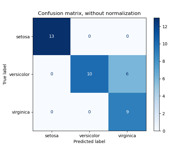
Параметр normalize позволяет сообщать коэффициенты вместо подсчетов. Матрица путаница может быть нормализована в 3 различными способами: 'pred', 'true'и 'all' которые будут делить счетчики на сумму каждого столбца, строки или всей матрицы, соответственно.
>>> y_true = [0, 0, 0, 1, 1, 1, 1, 1]
>>> y_pred = [0, 1, 0, 1, 0, 1, 0, 1]
>>> confusion_matrix(y_true, y_pred, normalize='all')
array([[0.25 , 0.125],
       [0.25 , 0.375]])
Для двоичных задач мы можем получить подсчет истинно отрицательных, ложноположительных, ложноотрицательных и истинно положительных результатов следующим образом:
>>> y_true = [0, 0, 0, 1, 1, 1, 1, 1]
>>> y_pred = [0, 1, 0, 1, 0, 1, 0, 1]
>>> tn, fp, fn, tp = confusion_matrix(y_true, y_pred).ravel()
>>> tn, fp, fn, tp
(2, 1, 2, 3)
Пример:
- См. В разделе Матрица неточностей пример использования матрицы неточностей для оценки качества выходных данных классификатора.
- См. В разделе Распознавание рукописных цифр пример использования матрицы неточностей для классификации рукописных цифр.
- См. Раздел Классификация текстовых документов с использованием разреженных функций для примера использования матрицы неточностей для классификации текстовых документов.
3.3.2.7. Отчет о классификации
Функция classification_report создает текстовый отчет , показывающий основные показатели классификации. Вот небольшой пример с настраиваемыми target_names и предполагаемыми ярлыками:
>>> from sklearn.metrics import classification_report
>>> y_true = [0, 1, 2, 2, 0]
>>> y_pred = [0, 0, 2, 1, 0]
>>> target_names = ['class 0', 'class 1', 'class 2']
>>> print(classification_report(y_true, y_pred, target_names=target_names))
              precision    recall  f1-score   support

     class 0       0.67      1.00      0.80         2
     class 1       0.00      0.00      0.00         1
     class 2       1.00      0.50      0.67         2

    accuracy                           0.60         5
   macro avg       0.56      0.50      0.49         5
weighted avg       0.67      0.60      0.59         5
Пример:
- См. В разделе Распознавание рукописных цифр пример использования отчета о классификации рукописных цифр.
- См. Раздел Классификация текстовых документов с использованием разреженных функций, где приведен пример использования отчета о классификации для текстовых документов.
- См. Раздел « Оценка параметров с использованием поиска по сетке с перекрестной проверкой», где приведен пример использования отчета о классификации для поиска по сетке с вложенной перекрестной проверкой.
3.3.2.8. Потеря Хэмминга
hamming_loss вычисляет среднюю потерю Хэмминга или расстояние Хемминга между двумя наборами образцов.
Если $hat{y}_j$ прогнозируемое значение для $j$-я этикетка данного образца, $y_j$ — соответствующее истинное значение, а $n_{labels}$ — количество классов или меток, то потеря Хэмминга $L_{Hamming}$ между двумя образцами определяется как:
$$L_{Hamming}(y, hat{y}) = frac{1}{n_text{labels}} sum_{j=0}^{n_text{labels} — 1} 1(hat{y}_j not= y_j)$$
где $1(x)$- индикаторная функция .
>>> from sklearn.metrics import hamming_loss
>>> y_pred = [1, 2, 3, 4]
>>> y_true = [2, 2, 3, 4]
>>> hamming_loss(y_true, y_pred)
0.25
В многопозиционном корпусе с бинарными индикаторами меток:
>>> hamming_loss(np.array([[0, 1], [1, 1]]), np.zeros((2, 2)))
0.75
Примечание
В мультиклассовой классификации потери Хэмминга соответствуют расстоянию Хэмминга между y_true и, y_pred что аналогично функции потерь нуля или единицы . Однако, в то время как потеря нуля или единицы наказывает наборы предсказаний, которые не строго соответствуют истинным наборам, потеря Хэмминга наказывает отдельные метки. Таким образом, потеря Хэмминга, ограниченная сверху потерей нуля или единицы, всегда находится между нулем и единицей включительно; и прогнозирование надлежащего подмножества или надмножества истинных меток даст исключительную потерю Хэмминга от нуля до единицы.
3.3.2.9. Точность, отзыв и F-меры
Интуитивно, точность — это способность классификатора не маркировать как положительный образец, который является отрицательным, а отзыв — это способность классификатора находить все положительные образцы.
F-мера ($F_beta$ а также $F_1$ меры) можно интерпретировать как взвешенное гармоническое среднее значение точности и полноты. А $F_beta$ мера достигает своего лучшего значения на уровне 1 и худшего результата на уровне 0. С $beta = 1$, $F_beta$ а также $F_1$ эквивалентны, а отзыв и точность одинаково важны.
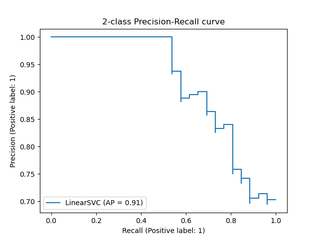
precision_recall_curve вычисляет кривую точности-отзыва на основе наземной метки истинности и оценки, полученной классификатором путем изменения порога принятия решения.
Функция average_precision_score вычисляет среднюю точность (AP) от оценки прогнозирования. Значение от 0 до 1 и выше — лучше. AP определяется как
$$text{AP} = sum_n (R_n — R_{n-1}) P_n$$
где $P_n$ а также $R_n$- точность и отзыв на n-м пороге. При случайных прогнозах AP — это доля положительных образцов.
Ссылки [Manning2008] и [Everingham2010] представляют альтернативные варианты AP, которые интерполируют кривую точности-отзыва. В настоящее время average_precision_score не реализован какой-либо вариант с интерполяцией. Ссылки [Davis2006] и [Flach2015] описывают, почему линейная интерполяция точек на кривой точности-отзыва обеспечивает чрезмерно оптимистичный показатель эффективности классификатора. Эта линейная интерполяция используется при вычислении площади под кривой с помощью правила трапеции в auc.
Несколько функций позволяют анализировать точность, отзыв и оценку F-мер:
average_precision_score(y_true, y_score, *) |
Вычислить среднюю точность (AP) из оценок прогнозов. |
f1_score(y_true, y_pred, *[, labels, …]) |
Вычислите оценку F1, также известную как сбалансированная оценка F или F-мера. |
fbeta_score(y_true, y_pred, *, beta[, …]) |
Вычислите оценку F-beta. |
precision_recall_curve(y_true, probas_pred, *) |
Вычислите пары точности-отзыва для разных пороговых значений вероятности. |
precision_recall_fscore_support(y_true, …) |
Точность вычислений, отзыв, F-мера и поддержка для каждого класса. |
precision_score(y_true, y_pred, *[, labels, …]) |
Вычислите точность. |
recall_score(y_true, y_pred, *[, labels, …]) |
Вычислите рекол. |
Обратите внимание, что функция precision_recall_curve ограничена двоичным регистром. Функция average_precision_score работает только в двоичном формате классификации и MultiLabel индикатора. В функции plot_precision_recall_curve графики точности вспомнить следующим образом .
Примеры:
- См. Раздел Классификация текстовых документов с использованием разреженных функций для примера использования
f1_scoreдля классификации текстовых документов. - См. Раздел « Оценка параметров с использованием поиска по сетке с перекрестной проверкой», где приведен пример
precision_scoreиrecall_scoreиспользование для оценки параметров с помощью поиска по сетке с вложенной перекрестной проверкой. - См. В разделе Precision-Recall пример использования
precision_recall_curveдля оценки качества вывода классификатора.
Рекомендации:
- [Manning2008] г. CD Manning, P. Raghavan, H. Schütze, Introduction to Information Retrieval , 2008.
- [Everingham2010] М. Эверингем, Л. Ван Гул, CKI Уильямс, Дж. Винн, А. Зиссерман, Задача классов визуальных объектов Pascal (VOC) , IJCV 2010.
- [Davis2006] Дж. Дэвис, М. Гоадрич, Взаимосвязь между точным воспроизведением и кривыми ROC , ICML 2006.
- [Flach2015] П.А. Флэч, М. Кулл, Кривые точности-отзыва-выигрыша: PR-анализ выполнен правильно , NIPS 2015.
3.3.2.9.1. Бинарная классификация
В задаче бинарной классификации термины «положительный» и «отрицательный» относятся к предсказанию классификатора, а термины «истинный» и «ложный» относятся к тому, соответствует ли этот прогноз внешнему суждению ( иногда известное как «наблюдение»). Учитывая эти определения, мы можем сформулировать следующую таблицу:
| Фактический класс (наблюдение) | ||
| Прогнозируемый класс (ожидание) | tp (истинно положительный результат) Правильный результат | fp (ложное срабатывание) Неожиданный результат |
| Прогнозируемый класс (ожидание) | fn (ложноотрицательный) Отсутствует результат | tn (истинно отрицательное) Правильное отсутствие результата |
В этом контексте мы можем определить понятия точности, отзыва и F-меры:
$$text{precision} = frac{tp}{tp + fp},$$
$$text{recall} = frac{tp}{tp + fn},$$
$$F_beta = (1 + beta^2) frac{text{precision} times text{recall}}{beta^2 text{precision} + text{recall}}.$$
Вот несколько небольших примеров бинарной классификации:
>>> from sklearn import metrics
>>> y_pred = [0, 1, 0, 0]
>>> y_true = [0, 1, 0, 1]
>>> metrics.precision_score(y_true, y_pred)
1.0
>>> metrics.recall_score(y_true, y_pred)
0.5
>>> metrics.f1_score(y_true, y_pred)
0.66...
>>> metrics.fbeta_score(y_true, y_pred, beta=0.5)
0.83...
>>> metrics.fbeta_score(y_true, y_pred, beta=1)
0.66...
>>> metrics.fbeta_score(y_true, y_pred, beta=2)
0.55...
>>> metrics.precision_recall_fscore_support(y_true, y_pred, beta=0.5)
(array([0.66..., 1.        ]), array([1. , 0.5]), array([0.71..., 0.83...]), array([2, 2]))


>>> import numpy as np
>>> from sklearn.metrics import precision_recall_curve
>>> from sklearn.metrics import average_precision_score
>>> y_true = np.array([0, 0, 1, 1])
>>> y_scores = np.array([0.1, 0.4, 0.35, 0.8])
>>> precision, recall, threshold = precision_recall_curve(y_true, y_scores)
>>> precision
array([0.66..., 0.5       , 1.        , 1.        ])
>>> recall
array([1. , 0.5, 0.5, 0. ])
>>> threshold
array([0.35, 0.4 , 0.8 ])
>>> average_precision_score(y_true, y_scores)
0.83...
3.3.2.9.2. Мультиклассовая и многозначная классификация
В задаче классификации по нескольким классам и меткам понятия точности, отзыва и F-меры могут применяться к каждой метке независимо. Есть несколько способов , чтобы объединить результаты по этикеткам, указанных в average аргументе к average_precision_score (MultiLabel только) f1_score, fbeta_score, precision_recall_fscore_support, precision_score и recall_score функция, как описано выше . Обратите внимание, что если включены все метки, «микро» -усреднение в настройке мультикласса обеспечит точность, отзыв и $F$ все они идентичны по точности. Также обратите внимание, что «взвешенное» усреднение может дать оценку F, которая не находится между точностью и отзывом.
Чтобы сделать это более явным, рассмотрим следующие обозначения:
- $y$ набор предсказанных ($sample$, $label$) пары
- $hat{y}$ набор истинных ($sample$, $label$) пары
- $L$ набор лейблов
- $S$ набор образцов
- $y_s$ подмножество $y$ с образцом $s$, т.е $y_s := left{(s’, l) in y | s’ = sright}$.
- $y_l$ подмножество $y$ с этикеткой $l$
- по аналогии, $hat{y}_s$ а также $hat{y}_l$ являются подмножествами $hat{y}$
- $P(A, B) := frac{left| A cap B right|}{left|Aright|}$ для некоторых наборов $A$ и $B$
- $R(A, B) := frac{left| A cap B right|}{left|Bright|}$ (Условные обозначения различаются в зависимости от обращения $B = emptyset$; эта реализация использует $R(A, B):=0$, и аналогичные для $P$.)
- $$F_beta(A, B) := left(1 + beta^2right) frac{P(A, B) times R(A, B)}{beta^2 P(A, B) + R(A, B)}$$
Тогда показатели определяются как:
| average | Точность | Отзывать | F_beta |
| «micro» | $P(y, hat{y})$ | $R(y, hat{y})$ | $F_beta(y, hat{y})$ |
| «samples» | $frac{1}{left|Sright|} sum_{s in S} P(y_s, hat{y}_s)$ | $frac{1}{left|Sright|} sum_{s in S} R(y_s, hat{y}_s)$ | $frac{1}{left|Sright|} sum_{s in S} F_beta(y_s, hat{y}_s)$ |
| «macro» | $frac{1}{left|Lright|} sum_{l in L} P(y_l, hat{y}_l)$ | $frac{1}{left|Lright|} sum_{l in L} R(y_l, hat{y}_l)$ | $frac{1}{left|Lright|} sum_{l in L} F_beta(y_l, hat{y}_l)$ |
| «weighted» | $frac{1}{sum_{l in L} left|hat{y}lright|} sum{l in L} left|hat{y}_lright| P(y_l, hat{y}_l)$ | $frac{1}{sum_{l in L} left|hat{y}lright|} sum{l in L} left|hat{y}_lright| R(y_l, hat{y}_l)$ | $frac{1}{sum_{l in L} left|hat{y}lright|} sum{l in L} left|hat{y}lright| Fbeta(y_l, hat{y}_l)$ |
| None | $langle P(y_l, hat{y}_l) | l in L rangle$ | $langle R(y_l, hat{y}_l) | l in L rangle$ | $langle F_beta(y_l, hat{y}_l) | l in L rangle$ |
>>> from sklearn import metrics
>>> y_true = [0, 1, 2, 0, 1, 2]
>>> y_pred = [0, 2, 1, 0, 0, 1]
>>> metrics.precision_score(y_true, y_pred, average='macro')
0.22...
>>> metrics.recall_score(y_true, y_pred, average='micro')
0.33...
>>> metrics.f1_score(y_true, y_pred, average='weighted')
0.26...
>>> metrics.fbeta_score(y_true, y_pred, average='macro', beta=0.5)
0.23...
>>> metrics.precision_recall_fscore_support(y_true, y_pred, beta=0.5, average=None)
(array([0.66..., 0.        , 0.        ]), array([1., 0., 0.]), array([0.71..., 0.        , 0.        ]), array([2, 2, 2]...))
Для мультиклассовой классификации с «отрицательным классом» можно исключить некоторые метки:
>>> metrics.recall_score(y_true, y_pred, labels=[1, 2], average='micro')
... # excluding 0, no labels were correctly recalled
0.0
Точно так же метки, отсутствующие в выборке данных, могут учитываться при макро-усреднении.
>>> metrics.precision_score(y_true, y_pred, labels=[0, 1, 2, 3], average='macro')
0.166...
3.3.2.10. Оценка коэффициента сходства Жаккара
Функция jaccard_score вычисляет среднее значение коэффициентов сходства Jaccard , также называемый индексом Jaccard, между парами множеств меток.
Коэффициент подобия Жаккара i-ые образцы, с набором меток наземной достоверности yi и прогнозируемый набор меток y^i, определяется как
$$J(y_i, hat{y}_i) = frac{|y_i cap hat{y}_i|}{|y_i cup hat{y}_i|}.$$
jaccard_score работает как precision_recall_fscore_support наивно установленная мера, применяемая изначально к бинарным целям, и расширена для применения к множественным меткам и мультиклассам за счет использования average(см. выше ).
В двоичном случае:
>>> import numpy as np
>>> from sklearn.metrics import jaccard_score
>>> y_true = np.array([[0, 1, 1],
...                    [1, 1, 0]])
>>> y_pred = np.array([[1, 1, 1],
...                    [1, 0, 0]])
>>> jaccard_score(y_true[0], y_pred[0])
0.6666...
В многопозиционном корпусе с бинарными индикаторами меток:
>>> jaccard_score(y_true, y_pred, average='samples')
0.5833...
>>> jaccard_score(y_true, y_pred, average='macro')
0.6666...
>>> jaccard_score(y_true, y_pred, average=None)
array([0.5, 0.5, 1. ])
Задачи с несколькими классами преобразуются в двоичную форму и обрабатываются как соответствующая задача с несколькими метками:
>>> y_pred = [0, 2, 1, 2]
>>> y_true = [0, 1, 2, 2]
>>> jaccard_score(y_true, y_pred, average=None)
array([1. , 0. , 0.33...])
>>> jaccard_score(y_true, y_pred, average='macro')
0.44...
>>> jaccard_score(y_true, y_pred, average='micro')
0.33...
3.3.2.11. Петля лосс
Функция hinge_loss вычисляет среднее расстояние между моделью и данными с использованием петля лосс, односторонний показателем , который учитывает только ошибки прогнозирования. (Потери на шарнирах используются в классификаторах максимальной маржи, таких как опорные векторные машины.)
Если метки закодированы с помощью +1 и -1, $y$: истинное значение, а $w$ — прогнозируемые решения на выходе decision_function, тогда потери на шарнирах определяются как:
$$L_text{Hinge}(y, w) = maxleft{1 — wy, 0right} = left|1 — wyright|_+$$
Если имеется более двух ярлыков, hinge_loss используется мультиклассовый вариант, разработанный Crammer & Singer. Вот статья, описывающая это.
Если $y_w$ прогнозируемое решение для истинного лейбла и $y_t$ — это максимум предсказанных решений для всех других меток, где предсказанные решения выводятся функцией принятия решений, тогда потеря шарнира в нескольких классах определяется следующим образом:
$$L_text{Hinge}(y_w, y_t) = maxleft{1 + y_t — y_w, 0right}$$
Вот небольшой пример, демонстрирующий использование hinge_loss функции с классификатором svm в задаче двоичного класса:
>>> from sklearn import svm
>>> from sklearn.metrics import hinge_loss
>>> X = [[0], [1]]
>>> y = [-1, 1]
>>> est = svm.LinearSVC(random_state=0)
>>> est.fit(X, y)
LinearSVC(random_state=0)
>>> pred_decision = est.decision_function([[-2], [3], [0.5]])
>>> pred_decision
array([-2.18...,  2.36...,  0.09...])
>>> hinge_loss([-1, 1, 1], pred_decision)
0.3...
Вот пример, демонстрирующий использование hinge_loss функции с классификатором svm в мультиклассовой задаче:
>>> X = np.array([[0], [1], [2], [3]])
>>> Y = np.array([0, 1, 2, 3])
>>> labels = np.array([0, 1, 2, 3])
>>> est = svm.LinearSVC()
>>> est.fit(X, Y)
LinearSVC()
>>> pred_decision = est.decision_function([[-1], [2], [3]])
>>> y_true = [0, 2, 3]
>>> hinge_loss(y_true, pred_decision, labels)
0.56...
3.3.2.12. Лог лосс
Лог лосс, также называемые потерями логистической регрессии или кросс-энтропийными потерями, определяются на основе оценок вероятности. Он обычно используется в (полиномиальной) логистической регрессии и нейронных сетях, а также в некоторых вариантах максимизации ожидания и может использоваться для оценки выходов вероятности ( predict_proba) классификатора вместо его дискретных прогнозов.
Для двоичной классификации с истинной меткой $y in {0,1}$ и оценка вероятности $p = operatorname{Pr}(y = 1)$, логарифмическая потеря на выборку представляет собой отрицательную логарифмическую вероятность классификатора с истинной меткой:
$$L_{log}(y, p) = -log operatorname{Pr}(y|p) = -(y log (p) + (1 — y) log (1 — p))$$
Это распространяется на случай мультикласса следующим образом. Пусть истинные метки для набора выборок будут закодированы размером 1 из K как двоичная индикаторная матрица $Y$, т.е. $y_{i,k}=1$ если образец $i$ есть ярлык $k$ взят из набора $K$ этикетки. Пусть $P$ — матрица оценок вероятностей, с $p_{i,k} = operatorname{Pr}(y_{i,k} = 1)$. Тогда потеря журнала всего набора равна
$$L_{log}(Y, P) = -log operatorname{Pr}(Y|P) = — frac{1}{N} sum_{i=0}^{N-1} sum_{k=0}^{K-1} y_{i,k} log p_{i,k}$$
Чтобы увидеть, как это обобщает приведенную выше потерю двоичного журнала, обратите внимание, что в двоичном случае $p_{i,0} = 1 — p_{i,1}$ и $y_{i,0} = 1 — y_{i,1}$, поэтому разложив внутреннюю сумму на $y_{i,k} in {0,1}$ дает двоичную потерю журнала.
В log_loss функции вычисляет журнал потеря дана список меток приземной истины и матриц вероятностей, возвращенный оценщик predict_proba методом.
>>> from sklearn.metrics import log_loss
>>> y_true = [0, 0, 1, 1]
>>> y_pred = [[.9, .1], [.8, .2], [.3, .7], [.01, .99]]
>>> log_loss(y_true, y_pred)
0.1738...
Первое [.9, .1] в y_pred означает 90% вероятность того, что первая выборка будет иметь метку 0. Лог лос неотрицательны.
3.3.2.13. Коэффициент корреляции Мэтьюза
Функция matthews_corrcoef вычисляет коэффициент корреляции Матфея (MCC) для двоичных классов. Цитата из Википедии:
«Коэффициент корреляции Мэтьюза используется в машинном обучении как мера качества двоичных (двухклассных) классификаций. Он учитывает истинные и ложные положительные и отрицательные результаты и обычно рассматривается как сбалансированная мера, которую можно использовать, даже если классы очень разных размеров. MCC — это, по сути, значение коэффициента корреляции между -1 и +1. Коэффициент +1 представляет собой идеальное предсказание, 0 — среднее случайное предсказание и -1 — обратное предсказание. Статистика также известна как коэффициент фи ».
В бинарном (двухклассовом) случае $tp$, $tn$, $fp$ а также $fn$ являются соответственно количеством истинно положительных, истинно отрицательных, ложноположительных и ложноотрицательных результатов, MCC определяется как
$$MCC = frac{tp times tn — fp times fn}{sqrt{(tp + fp)(tp + fn)(tn + fp)(tn + fn)}}.$$
В случае мультикласса коэффициент корреляции Мэтьюза может быть определен в терминах confusion_matrix C для Kклассы. Чтобы упростить определение, рассмотрим следующие промежуточные переменные:
- $t_k=sum_{i}^{K} C_{ik}$ количество занятий k действительно произошло,
- $p_k=sum_{i}^{K} C_{ki}$ количество занятий k был предсказан,
- $c=sum_{k}^{K} C_{kk}$ общее количество правильно спрогнозированных образцов,
- $s=sum_{i}^{K} sum_{j}^{K} C_{ij}$ общее количество образцов.
Тогда мультиклассовый MCC определяется как:
$$MCC = frac{ c times s — sum_{k}^{K} p_k times t_k }{sqrt{ (s^2 — sum_{k}^{K} p_k^2) times (s^2 — sum_{k}^{K} t_k^2) }}$$
Когда имеется более двух меток, значение MCC больше не будет находиться в диапазоне от -1 до +1. Вместо этого минимальное значение будет где-то между -1 и 0 в зависимости от количества и распределения наземных истинных меток. Максимальное значение всегда +1.
Вот небольшой пример, иллюстрирующий использование matthews_corrcoef функции:
>>> from sklearn.metrics import matthews_corrcoef
>>> y_true = [+1, +1, +1, -1]
>>> y_pred = [+1, -1, +1, +1]
>>> matthews_corrcoef(y_true, y_pred)
-0.33...
3.3.2.14. Матрица путаницы с несколькими метками
Функция multilabel_confusion_matrix вычисляет класс-накрест ( по умолчанию) или samplewise (samplewise = True) MultiLabel матрицы спутанности для оценки точности классификации. Multilabel_confusion_matrix также обрабатывает данные мультикласса, как если бы они были многоклассовыми, поскольку это преобразование, обычно применяемое для оценки проблем мультикласса с метриками двоичной классификации (такими как точность, отзыв и т. д.).
При вычислении классовой матрицы путаницы с несколькими метками $C$, количество истинных негативов для класса i является $C_{i,0,0}$, ложноотрицательные $C_{i,1,0}$, истинные положительные стороны $C_{i,1,1}$ а ложные срабатывания $C_{i,0,1}$.
Вот пример, демонстрирующий использование multilabel_confusion_matrix функции с вводом многозначной индикаторной матрицы:
>>> import numpy as np
>>> from sklearn.metrics import multilabel_confusion_matrix
>>> y_true = np.array([[1, 0, 1],
...                    [0, 1, 0]])
>>> y_pred = np.array([[1, 0, 0],
...                    [0, 1, 1]])
>>> multilabel_confusion_matrix(y_true, y_pred)
array([[[1, 0],
        [0, 1]],

       [[1, 0],
        [0, 1]],

       [[0, 1],
        [1, 0]]])
Или можно построить матрицу неточностей для каждой метки образца:
>>> multilabel_confusion_matrix(y_true, y_pred, samplewise=True)
array([[[1, 0],
        [1, 1]],

       [[1, 1],
        [0, 1]]])
Вот пример, демонстрирующий использование multilabel_confusion_matrix функции с многоклассовым вводом:
>>> y_true = ["cat", "ant", "cat", "cat", "ant", "bird"]
>>> y_pred = ["ant", "ant", "cat", "cat", "ant", "cat"]
>>> multilabel_confusion_matrix(y_true, y_pred,
...                             labels=["ant", "bird", "cat"])
array([[[3, 1],
        [0, 2]],

       [[5, 0],
        [1, 0]],

       [[2, 1],
        [1, 2]]])
Вот несколько примеров, демонстрирующих использование multilabel_confusion_matrix функции для расчета отзыва (или чувствительности), специфичности, количества выпадений и пропусков для каждого класса в задаче с вводом многозначной индикаторной матрицы.
Расчет отзыва (также называемого истинно положительным коэффициентом или чувствительностью) для каждого класса:
>>> y_true = np.array([[0, 0, 1],
...                    [0, 1, 0],
...                    [1, 1, 0]])
>>> y_pred = np.array([[0, 1, 0],
...                    [0, 0, 1],
...                    [1, 1, 0]])
>>> mcm = multilabel_confusion_matrix(y_true, y_pred)
>>> tn = mcm[:, 0, 0]
>>> tp = mcm[:, 1, 1]
>>> fn = mcm[:, 1, 0]
>>> fp = mcm[:, 0, 1]
>>> tp / (tp + fn)
array([1. , 0.5, 0. ])
Расчет специфичности (также называемой истинно отрицательной ставкой) для каждого класса:
>>> tn / (tn + fp)
array([1. , 0. , 0.5])
Расчет количества выпадений (также называемый частотой ложных срабатываний) для каждого класса:
>>> fp / (fp + tn)
array([0. , 1. , 0.5])
Расчет процента промахов (также называемого ложноотрицательным показателем) для каждого класса:
>>> fn / (fn + tp)
array([0. , 0.5, 1. ])
3.3.2.15. Рабочая характеристика приемника (ROC)
Функция roc_curve вычисляет рабочую характеристическую кривую приемника или кривую ROC . Цитата из Википедии:
«Рабочая характеристика приемника (ROC), или просто кривая ROC, представляет собой графический график, который иллюстрирует работу системы двоичного классификатора при изменении ее порога дискриминации. Он создается путем построения графика доли истинных положительных результатов из положительных (TPR = частота истинных положительных результатов) по сравнению с долей ложных положительных результатов из отрицательных (FPR = частота ложных положительных результатов) при различных настройках пороговых значений. TPR также известен как чувствительность, а FPR — это единица минус специфичность или истинно отрицательный показатель ».
Для этой функции требуется истинное двоичное значение и целевые баллы, которые могут быть либо оценками вероятности положительного класса, либо значениями достоверности, либо двоичными решениями. Вот небольшой пример использования roc_curve функции:
>>> import numpy as np
>>> from sklearn.metrics import roc_curve
>>> y = np.array([1, 1, 2, 2])
>>> scores = np.array([0.1, 0.4, 0.35, 0.8])
>>> fpr, tpr, thresholds = roc_curve(y, scores, pos_label=2)
>>> fpr
array([0. , 0. , 0.5, 0.5, 1. ])
>>> tpr
array([0. , 0.5, 0.5, 1. , 1. ])
>>> thresholds
array([1.8 , 0.8 , 0.4 , 0.35, 0.1 ])
На этом рисунке показан пример такой кривой ROC:
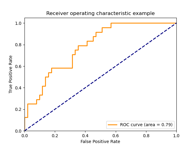
Функция roc_auc_score вычисляет площадь под операционной приемника характеристика (ROC) кривой, которая также обозначается через ППК или AUROC. При вычислении площади под кривой roc информация о кривой суммируется в одном номере. Для получения дополнительной информации см. Статью в Википедии о AUC.
По сравнению с такими показателями, как точность подмножества, потеря Хэмминга или оценка F1, ROC не требует оптимизации порога для каждой метки.
3.3.2.15.1. Двоичный регистр
В двоичном случае вы можете либо предоставить оценки вероятности, используя classifier.predict_proba() метод, либо значения решения без пороговых значений, заданные classifier.decision_function() методом. В случае предоставления оценок вероятности следует указать вероятность класса с «большей меткой». «Большая метка» соответствует classifier.classes_[1] и, следовательно classifier.predict_proba(X) [:, 1]. Следовательно, параметр y_score имеет размер (n_samples,).
>>> from sklearn.datasets import load_breast_cancer
>>> from sklearn.linear_model import LogisticRegression
>>> from sklearn.metrics import roc_auc_score
>>> X, y = load_breast_cancer(return_X_y=True)
>>> clf = LogisticRegression(solver="liblinear").fit(X, y)
>>> clf.classes_
array([0, 1])
Мы можем использовать оценки вероятностей, соответствующие clf.classes_[1].
>>> y_score = clf.predict_proba(X)[:, 1]
>>> roc_auc_score(y, y_score)
0.99...
В противном случае мы можем использовать значения решения без порога.
>>> roc_auc_score(y, clf.decision_function(X))
0.99...
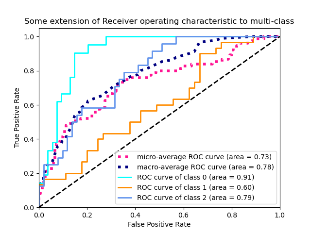
3.3.2.15.2. Мультиклассовый кейс
Функция roc_auc_score также может быть использована в нескольких классах классификации . В настоящее время поддерживаются две стратегии усреднения: алгоритм «один против одного» вычисляет среднее попарных оценок AUC ROC, а алгоритм «один против остальных» вычисляет среднее значение оценок ROC AUC для каждого класса по сравнению со всеми другими классами. В обоих случаях предсказанные метки предоставляются в виде массива со значениями от 0 до n_classes, а оценки соответствуют оценкам вероятности того, что выборка принадлежит определенному классу. Алгоритмы OvO и OvR поддерживают равномерное взвешивание ( average='macro') и по распространенности ( average='weighted').
Алгоритм «один против одного» : вычисляет средний AUC всех возможных попарных комбинаций классов. [HT2001] определяет метрику AUC мультикласса, взвешенную равномерно:
$$frac{1}{c(c-1)}sum_{j=1}^{c}sum_{k > j}^c (text{AUC}(j | k) + text{AUC}(k | j))$$
где $c$ количество классов и $text{AUC}(j | k)$ AUC с классом $j$ как положительный класс и класс $k$ как отрицательный класс. В общем, $text{AUC}(j | k) neq text{AUC}(k | j))$ в случае мультикласса. Этот алгоритм используется, установив аргумент ключевого слова , multiclass чтобы 'ovo' и average в 'macro'.
[HT2001] мультиклассируют AUC метрика может быть расширена , чтобы быть взвешены по распространенности:
$$frac{1}{c(c-1)}sum_{j=1}^{c}sum_{k > j}^c p(j cup k)( text{AUC}(j | k) + text{AUC}(k | j))$$
где cколичество классов. Этот алгоритм используется, установив аргумент ключевого слова , multiclass чтобы 'ovo' и average в 'weighted'. В 'weighted' опции возвращает распространенность усредненные , как описано в [FC2009] .
Алгоритм «один против остальных» : вычисляет AUC каждого класса относительно остальных [PD2000] . Алгоритм функционально такой же, как и в случае с несколькими этикетками. Чтобы включить этот алгоритм, установите для аргумента ключевого слова multiclass значение 'ovr'. Как и OvO, OvR поддерживает два типа усреднения: 'macro' [F2006] и 'weighted' [F2001] .
В приложениях , где высокий процент ложных срабатываний не терпимый параметр max_fpr из roc_auc_score может быть использовано , чтобы суммировать кривую ROC до заданного предела.
3.3.2.15.3. Кейс с несколькими метками
В классификации несколько меток, функция roc_auc_score распространяются путем усреднения меток , как выше . В этом случае вы должны указать y_score форму . Таким образом, при использовании оценок вероятности необходимо выбрать вероятность класса с большей меткой для каждого выхода.(n_samples, n_classes)
>>> from sklearn.datasets import make_multilabel_classification
>>> from sklearn.multioutput import MultiOutputClassifier
>>> X, y = make_multilabel_classification(random_state=0)
>>> inner_clf = LogisticRegression(solver="liblinear", random_state=0)
>>> clf = MultiOutputClassifier(inner_clf).fit(X, y)
>>> y_score = np.transpose([y_pred[:, 1] for y_pred in clf.predict_proba(X)])
>>> roc_auc_score(y, y_score, average=None)
array([0.82..., 0.86..., 0.94..., 0.85... , 0.94...])
И значения решений не требуют такой обработки.
>>> from sklearn.linear_model import RidgeClassifierCV
>>> clf = RidgeClassifierCV().fit(X, y)
>>> y_score = clf.decision_function(X)
>>> roc_auc_score(y, y_score, average=None)
array([0.81..., 0.84... , 0.93..., 0.87..., 0.94...])
Примеры:
- См. В разделе « Рабочие характеристики приемника» (ROC) пример использования ROC для оценки качества выходных данных классификатора.
- См. В разделе « Рабочие характеристики приемника» (ROC) с перекрестной проверкой пример использования ROC для оценки качества выходных данных классификатора с помощью перекрестной проверки.
- См. В разделе Моделирование распределения видов пример использования ROC для моделирования распределения видов.
- HT2001 ( 1 , 2 ) Рука, DJ и Тилль, RJ, (2001). Простое обобщение области под кривой ROC для задач классификации нескольких классов. Машинное обучение, 45 (2), стр. 171-186.
- FC2009 Ферри, Сезар и Эрнандес-Оралло, Хосе и Модройу, Р. (2009). Экспериментальное сравнение показателей эффективности для классификации. Письма о распознавании образов. 30. 27-38.
- PD2000 Провост Ф., Домингос П. (2000). Хорошо обученные ПЭТ: Улучшение деревьев оценки вероятностей (Раздел 6.2), Рабочий документ CeDER № IS-00-04, Школа бизнеса Стерна, Нью-Йоркский университет.
- F2006 Фосетт, Т., 2006. Введение в анализ ROC. Письма о распознавании образов, 27 (8), стр. 861-874.
- F2001Фосетт, Т., 2001. Использование наборов правил для максимизации производительности ROC в интеллектуальном анализе данных, 2001. Труды Международной конференции IEEE, стр. 131-138.
3.3.2.16. Компромисс при обнаружении ошибок (DET)
Функция det_curve вычисляет кривую компенсации ошибок обнаружения (DET) [WikipediaDET2017] . Цитата из Википедии:
«График компромисса ошибок обнаружения (DET) — это графическая диаграмма частоты ошибок для систем двоичной классификации, отображающая частоту ложных отклонений по сравнению с частотой ложных приемов. Оси x и y масштабируются нелинейно по их стандартным нормальным отклонениям (или просто с помощью логарифмического преобразования), в результате получаются более линейные кривые компромисса, чем кривые ROC, и большая часть области изображения используется для выделения важных различий в критический рабочий регион ».
Кривые DET представляют собой вариацию кривых рабочих характеристик приемника (ROC), где ложная отрицательная скорость нанесена на ось y вместо истинной положительной скорости. Кривые DET обычно строятся в масштабе нормального отклонения путем преобразования $phi^{-1}$ (с участием $phi$ — кумулятивная функция распределения). Полученные кривые производительности явно визуализируют компромисс типов ошибок для заданных алгоритмов классификации. См. [Martin1997], где приведены примеры и мотивация.
На этом рисунке сравниваются кривые ROC и DET двух примеров классификаторов для одной и той же задачи классификации:
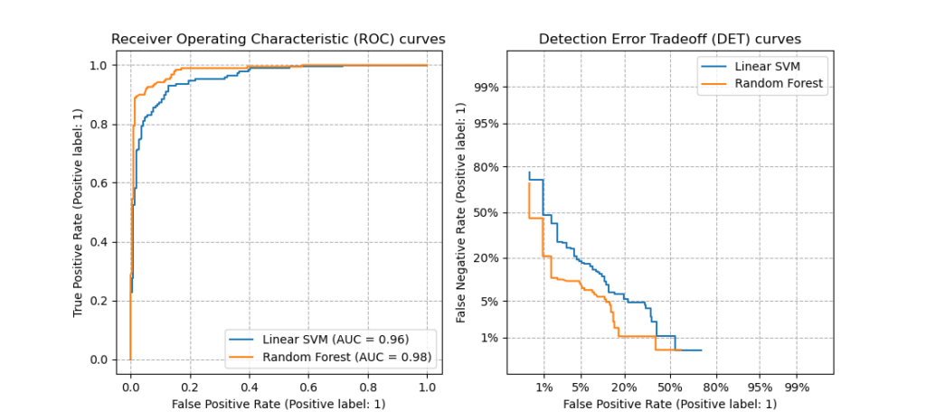
Характеристики:
- Кривые DET образуют линейную кривую по шкале нормального отклонения, если оценки обнаружения нормально (или близки к нормальному) распределены. В [Navratil2007] было показано, что обратное не обязательно верно, и даже более общие распределения могут давать линейные кривые DET.
- При обычном преобразовании масштаба с отклонением точки распределяются таким образом, что занимает сравнительно большее пространство графика. Следовательно, кривые с аналогичными характеристиками классификации легче различить на графике DET.
- С ложноотрицательной скоростью, «обратной» истинной положительной скорости, точкой совершенства для кривых DET является начало координат (в отличие от верхнего левого угла для кривых ROC).
Приложения и ограничения:
Кривые DET интуитивно понятны для чтения и, следовательно, позволяют быстро визуально оценить работу классификатора. Кроме того, кривые DET можно использовать для анализа пороговых значений и выбора рабочей точки. Это особенно полезно, если требуется сравнение типов ошибок.
С другой стороны, кривые DET не представляют свою метрику в виде единого числа. Поэтому для автоматической оценки или сравнения с другими задачами классификации лучше подходят такие показатели, как производная площадь под кривой ROC.
Примеры:
- См. Кривую компенсации ошибок обнаружения (DET) для примера сравнения кривых рабочих характеристик приемника (ROC) и кривых компенсации ошибок обнаружения (DET).
Рекомендации:
- ВикипедияDET2017 Авторы Википедии. Компромисс ошибки обнаружения. Википедия, свободная энциклопедия. 4 сентября 2017 г., 23:33 UTC. Доступно по адресу: https://en.wikipedia.org/w/index.php?title=Detection_error_tradeoff&oldid=798982054 . По состоянию на 19 февраля 2018 г.
- Мартин 1997 А. Мартин, Дж. Доддингтон, Т. Камм, М. Ордовски и М. Пшибоцки, Кривая DET в оценке эффективности задач обнаружения , NIST 1997.
- Навратил2007 Дж. Наврактил и Д. Клусачек, « О линейных DET », 2007 г. Международная конференция IEEE по акустике, обработке речи и сигналов — ICASSP ’07, Гонолулу, Гавайи, 2007 г., стр. IV-229-IV-232.
3.3.2.17. Нулевой проигрыш
Функция zero_one_loss вычисляет сумму или среднее значение потери 0-1 классификации ($L_{0−1}$) над $n_{samples}$. По умолчанию функция нормализуется по выборке. Чтобы получить сумму $L_{0−1}$, установите normalize значение False.
В классификации по zero_one_loss нескольким меткам подмножество оценивается как единое целое, если его метки строго соответствуют прогнозам, и как ноль, если есть какие-либо ошибки. По умолчанию функция возвращает процент неправильно спрогнозированных подмножеств. Чтобы вместо этого получить количество таких подмножеств, установите normalize значение False
Если $hat{y}_i$ прогнозируемое значение $i$-й образец и $y_i$ — соответствующее истинное значение, тогда потеря 0-1 $L_{0−1}$ определяется как:
$$L_{0-1}(y_i, hat{y}_i) = 1(hat{y}_i not= y_i)$$
где $1(x)$- индикаторная функция.
>>> from sklearn.metrics import zero_one_loss
>>> y_pred = [1, 2, 3, 4]
>>> y_true = [2, 2, 3, 4]
>>> zero_one_loss(y_true, y_pred)
0.25
>>> zero_one_loss(y_true, y_pred, normalize=False)
1
В случае с несколькими метками с двоичными индикаторами меток, где первый набор меток [0,1] содержит ошибку:
>>> zero_one_loss(np.array([[0, 1], [1, 1]]), np.ones((2, 2)))
0.5

>>> zero_one_loss(np.array([[0, 1], [1, 1]]), np.ones((2, 2)),  normalize=False)
1
Пример:
- См. В разделе « Рекурсивное исключение функции с перекрестной проверкой» пример использования нулевой потери для выполнения рекурсивного исключения функции с перекрестной проверкой.
3.3.2.18. Потеря очков по Брайеру
Функция brier_score_loss вычисляет оценку Шиповник для бинарных классов [Brier1950] . Цитата из Википедии:
«Оценка Бриера — это правильная функция оценки, которая измеряет точность вероятностных прогнозов. Это применимо к задачам, в которых прогнозы должны назначать вероятности набору взаимоисключающих дискретных результатов ».
Эта функция возвращает среднеквадратичную ошибку фактического результата. y∈{0,1} и прогнозируемая оценка вероятности $p=Pr(y=1)$ ( pred_proba ) как выведено :
$$BS = frac{1}{n_{text{samples}}} sum_{i=0}^{n_{text{samples}} — 1}(y_i — p_i)^2$$
Потеря по шкале Бриера также составляет от 0 до 1, и чем ниже значение (средняя квадратичная разница меньше), тем точнее прогноз.
Вот небольшой пример использования этой функции:
>>> import numpy as np
>>> from sklearn.metrics import brier_score_loss
>>> y_true = np.array([0, 1, 1, 0])
>>> y_true_categorical = np.array(["spam", "ham", "ham", "spam"])
>>> y_prob = np.array([0.1, 0.9, 0.8, 0.4])
>>> y_pred = np.array([0, 1, 1, 0])
>>> brier_score_loss(y_true, y_prob)
0.055
>>> brier_score_loss(y_true, 1 - y_prob, pos_label=0)
0.055
>>> brier_score_loss(y_true_categorical, y_prob, pos_label="ham")
0.055
>>> brier_score_loss(y_true, y_prob > 0.5)
0.0
Балл Бриера можно использовать для оценки того, насколько хорошо откалиброван классификатор. Однако меньшая потеря по шкале Бриера не всегда означает лучшую калибровку. Это связано с тем, что по аналогии с разложением среднеквадратичной ошибки на дисперсию смещения потеря оценки по Бриеру может быть разложена как сумма потерь калибровки и потерь при уточнении [Bella2012]. Потеря калибровки определяется как среднеквадратическое отклонение от эмпирических вероятностей, полученных из наклона ROC-сегментов. Потери при переработке можно определить как ожидаемые оптимальные потери, измеренные по площади под кривой оптимальных затрат. Потери при уточнении могут изменяться независимо от потерь при калибровке, таким образом, более низкие потери по шкале Бриера не обязательно означают более качественную калибровку модели. «Только когда потеря точности остается неизменной, более низкая потеря по шкале Бриера всегда означает лучшую калибровку» [Bella2012] , [Flach2008] .
Пример:
- См. Раздел « Калибровка вероятности классификаторов», где приведен пример использования потерь по шкале Бриера для выполнения калибровки вероятности классификаторов.
Рекомендации:
- Brier1950 Дж. Брайер, Проверка прогнозов, выраженных в терминах вероятности , Ежемесячный обзор погоды 78.1 (1950)
- Bella2012 ( 1 , 2 ) Белла, Ферри, Эрнандес-Оралло и Рамирес-Кинтана «Калибровка моделей машинного обучения» в Хосров-Пур, М. «Машинное обучение: концепции, методологии, инструменты и приложения». Херши, Пенсильвания: Справочник по информационным наукам (2012).
- Flach2008 Флак, Питер и Эдсон Мацубара. «О классификации, ранжировании и оценке вероятности». Дагштульский семинар. Schloss Dagstuhl-Leibniz-Zentrum от Informatik (2008).
3.3.3. Метрики ранжирования с несколькими ярлыками
В многоэлементном обучении с каждой выборкой может быть связано любое количество меток истинности. Цель состоит в том, чтобы дать высокие оценки и более высокий рейтинг наземным лейблам.
3.3.3.1. Ошибка покрытия
Функция coverage_error вычисляет среднее число меток , которые должны быть включены в окончательном предсказании таким образом, что все истинные метки предсказанные. Это полезно, если вы хотите знать, сколько меток с наивысшими баллами вам нужно предсказать в среднем, не пропуская ни одной истинной. Таким образом, наилучшее значение этого показателя — среднее количество истинных ярлыков.
Примечание
Оценка нашей реализации на 1 больше, чем оценка, приведенная в Tsoumakas et al., 2010. Это расширяет ее для обработки вырожденного случая, когда экземпляр имеет 0 истинных меток.
Формально, учитывая двоичную индикаторную матрицу наземных меток истинности $y in left{0, 1right}^{n_text{samples} times n_text{labels}}$ и оценка, связанная с каждой меткой $hat{f} in mathbb{R}^{n_text{samples} times n_text{labels}}$ покрытие определяется как
$$coverage(y, hat{f}) = frac{1}{n_{text{samples}}} sum_{i=0}^{n_{text{samples}} — 1} max_{j:y_{ij} = 1} text{rank}_{ij}$$
с участием $text{rank}{ij} = left|left{k: hat{f}{ik} geq hat{f}_{ij} right}right|$. Учитывая определение ранга, связи y_scores разрываются путем присвоения максимального ранга, который был бы присвоен всем связанным значениям.
Вот небольшой пример использования этой функции:
>>> import numpy as np
>>> from sklearn.metrics import coverage_error
>>> y_true = np.array([[1, 0, 0], [0, 0, 1]])
>>> y_score = np.array([[0.75, 0.5, 1], [1, 0.2, 0.1]])
>>> coverage_error(y_true, y_score)
2.5
3.3.3.2. Средняя точность ранжирования метки
В label_ranking_average_precision_score функции реализует маркировать ранжирование средней точности (LRAP). Этот показатель связан с average_precision_score функцией, но основан на понятии ранжирования меток, а не на точности и отзыве.
Средняя точность ранжирования меток (LRAP) усредняет по выборкам ответ на следующий вопрос: для каждой основной метки истинности какая доля меток с более высоким рейтингом была истинной? Этот показатель эффективности будет выше, если вы сможете лучше ранжировать метки, связанные с каждым образцом. Полученная оценка всегда строго больше 0, а наилучшее значение равно 1. Если имеется ровно одна релевантная метка для каждой выборки, средняя точность ранжирования меток эквивалентна среднему обратному рангу .
Формально, учитывая двоичную индикаторную матрицу наземных меток истинности $y in left{0, 1right}^{n_text{samples} times n_text{labels}}$ и оценка, связанная с каждой меткой $hat{f} in mathbb{R}^{n_text{samples} times n_text{labels}}$, средняя точность определяется как
$$LRAP(y, hat{f}) = frac{1}{n_{text{samples}}} sum_{i=0}^{n_{text{samples}} — 1} frac{1}{||y_i||0} sum{j:y_{ij} = 1} frac{|mathcal{L}{ij}|}{text{rank}{ij}}$$
где $mathcal{L}{ij} = left{k: y{ik} = 1, hat{f}{ik} geq hat{f}{ij} right}$, $text{rank}{ij} = left|left{k: hat{f}{ik} geq hat{f}_{ij} right}right|$, |cdot| вычисляет мощность набора (т. е. количество элементов в наборе), и $||cdot||_0$ это $ell_0$ «Norm» (который вычисляет количество ненулевых элементов в векторе).
Вот небольшой пример использования этой функции:
>>> import numpy as np
>>> from sklearn.metrics import label_ranking_average_precision_score
>>> y_true = np.array([[1, 0, 0], [0, 0, 1]])
>>> y_score = np.array([[0.75, 0.5, 1], [1, 0.2, 0.1]])
>>> label_ranking_average_precision_score(y_true, y_score)
0.416...
3.3.3.3. Потеря рейтинга
Функция label_ranking_loss вычисляет ранжирование потери , которые в среднем более образцы числа пар меток, которые неправильно упорядочены, т.е. истинные метки имеют более низкую оценку , чем ложные метки, взвешенную по обратной величине числа упорядоченных пар ложных и истинных меток. Наименьшая возможная потеря рейтинга равна нулю.
Формально, учитывая двоичную индикаторную матрицу наземных меток истинности $y in left{0, 1right}^{n_text{samples} times n_text{labels}}$ и оценка, связанная с каждой меткой $hat{f} in mathbb{R}^{n_text{samples} times n_text{labels}}$ потеря ранжирования определяется как
$$ranking_loss(y, hat{f}) = frac{1}{n_{text{samples}}} sum_{i=0}^{n_{text{samples}} — 1} frac{1}{||y_i||0(ntext{labels} — ||y_i||0)} left|left{(k, l): hat{f}{ik} leq hat{f}{il}, y{ik} = 1, y_{il} = 0 right}right|$$
где $|cdot|$ вычисляет мощность набора (т. е. количество элементов в наборе) и $||cdot||_0$ это $ell_0$ «Norm» (который вычисляет количество ненулевых элементов в векторе).
Вот небольшой пример использования этой функции:
>>> import numpy as np
>>> from sklearn.metrics import label_ranking_loss
>>> y_true = np.array([[1, 0, 0], [0, 0, 1]])
>>> y_score = np.array([[0.75, 0.5, 1], [1, 0.2, 0.1]])
>>> label_ranking_loss(y_true, y_score)
0.75...
>>> # With the following prediction, we have perfect and minimal loss
>>> y_score = np.array([[1.0, 0.1, 0.2], [0.1, 0.2, 0.9]])
>>> label_ranking_loss(y_true, y_score)
0.0
Рекомендации:
- Цумакас, Г., Катакис, И., и Влахавас, И. (2010). Майнинг данных с несколькими метками. В справочнике по интеллектуальному анализу данных и открытию знаний (стр. 667-685). Springer США.
3.3.3.4. Нормализованная дисконтированная совокупная прибыль
Дисконтированный совокупный выигрыш (DCG) и Нормализованный дисконтированный совокупный выигрыш (NDCG) — это показатели ранжирования, реализованные в dcg_score и ndcg_score; они сравнивают предсказанный порядок с оценками достоверности, такими как релевантность ответов на запрос.
Со страницы Википедии о дисконтированной совокупной прибыли:
«Дисконтированная совокупная прибыль (DCG) — это показатель качества ранжирования. При поиске информации он часто используется для измерения эффективности алгоритмов поисковой системы или связанных приложений. Используя шкалу градуированной релевантности документов в наборе результатов поисковой системы, DCG измеряет полезность или выгоду документа на основе его позиции в списке результатов. Прирост накапливается сверху вниз в списке результатов, причем прирост каждого результата дисконтируется на более низких уровнях »
DCG упорядочивает истинные цели (например, релевантность ответов на запросы) в предсказанном порядке, затем умножает их на логарифмическое убывание и суммирует результат. Сумма может быть усечена после первогоKрезультатов, и в этом случае мы называем это DCG @ K. NDCG или NDCG @ $K$ — это DCG, деленная на DCG, полученную с помощью точного прогноза, так что оно всегда находится между 0 и 1. Обычно NDCG предпочтительнее DCG.
По сравнению с потерей ранжирования, NDCG может принимать во внимание оценки релевантности, а не ранжирование на основе фактов. Таким образом, если основополагающая информация состоит только из упорядочивания, предпочтение следует отдавать потере ранжирования; если основополагающая информация состоит из фактических оценок полезности (например, 0 для нерелевантного, 1 для релевантного, 2 для очень актуального), можно использовать NDCG.
Для одного образца, учитывая вектор непрерывных значений истинности для каждой цели $y in R^M$, где $M$ это количество выходов, а прогноз $hat{y}$, что индуцирует функцию ранжирования $f$, оценка DCG составляет
$$sum_{r=1}^{min(K, M)}frac{y_{f(r)}}{log(1 + r)}$$
а оценка NDCG — это оценка DCG, деленная на оценку DCG, полученную для $y$.
Рекомендации:
- Запись в Википедии о дисконтированной совокупной прибыли
- Джарвелин, К., и Кекалайнен, Дж. (2002). Оценка IR методов на основе накопленного коэффициента усиления. Транзакции ACM в информационных системах (TOIS), 20 (4), 422-446.
- Ван, Ю., Ван, Л., Ли, Ю., Хе, Д., Чен, В., и Лю, Т. Ю. (2013, май). Теоретический анализ показателей рейтинга NDCG. В материалах 26-й ежегодной конференции по теории обучения (COLT 2013)
- МакШерри Ф. и Наджорк М. (2008, март). Эффективность вычислений при поиске информации измеряется эффективно при наличии связанных оценок. В Европейской конференции по поиску информации (стр. 414-421). Шпрингер, Берлин, Гейдельберг.
3.3.4. Метрики регрессии
В sklearn.metrics модуле реализованы несколько функций потерь, оценки и полезности для измерения эффективности регрессии. Некоторые из них были расширены , чтобы обработать случай multioutput: mean_squared_error, mean_absolute_error, explained_variance_score и r2_score.
У этих функций есть multioutput аргумент ключевого слова, который определяет способ усреднения результатов или проигрышей для каждой отдельной цели. По умолчанию используется значение 'uniform_average', которое определяет равномерно взвешенное среднее значение по выходным данным. Если передается ndarrayформа shape (n_outputs,), то ее записи интерпретируются как веса, и возвращается соответствующее средневзвешенное значение. Если multioutputесть 'raw_values'указан, то все неизменные индивидуальные баллы или потери будут возвращены в массиве формы (n_outputs,).
r2_score и explained_variance_score принять дополнительное значение 'variance_weighted' для multioutput параметра. Эта опция приводит к взвешиванию каждой индивидуальной оценки по дисперсии соответствующей целевой переменной. Этот параметр определяет количественно зафиксированную немасштабированную дисперсию на глобальном уровне. Если целевые переменные имеют разную шкалу, то этот балл придает большее значение хорошему объяснению переменных с более высокой дисперсией. multioutput='variance_weighted' — значение по умолчанию r2_score для обратной совместимости. В будущем это будет изменено на uniform_average.
3.3.4.1. Оценка объясненной дисперсии
explained_variance_score вычисляет объясненной дисперсии регрессии балл.
Если $hat{y}$ — расчетный целевой объем производства, y соответствующий (правильный) целевой результат, и $Var$- Дисперсия , квадрат стандартного отклонения, то объясненная дисперсия оценивается следующим образом:
$$explained_{}variance(y, hat{y}) = 1 — frac{Var{ y — hat{y}}}{Var{y}}$$
Наилучшая возможная оценка — 1.0, более низкие значения — хуже.
Вот небольшой пример использования explained_variance_score функции:
>>> from sklearn.metrics import explained_variance_score
>>> y_true = [3, -0.5, 2, 7]
>>> y_pred = [2.5, 0.0, 2, 8]
>>> explained_variance_score(y_true, y_pred)
0.957...
>>> y_true = [[0.5, 1], [-1, 1], [7, -6]]
>>> y_pred = [[0, 2], [-1, 2], [8, -5]]
>>> explained_variance_score(y_true, y_pred, multioutput='raw_values')
array([0.967..., 1.        ])
>>> explained_variance_score(y_true, y_pred, multioutput=[0.3, 0.7])
0.990...
3.3.4.2. Максимальная ошибка
Функция max_error вычисляет максимальную остаточную ошибку , показатель , который фиксирует худшую ошибку случае между предсказанным значением и истинным значением. В идеально подобранной модели регрессии с одним выходом он max_error будет находиться 0 в обучающем наборе, и хотя это маловероятно в реальном мире, этот показатель показывает степень ошибки, которую имела модель при подборе.
Если $hat{y}_i$ прогнозируемое значение $i$-й образец, и $y_i$ — соответствующее истинное значение, тогда максимальная ошибка определяется как
$$text{Max Error}(y, hat{y}) = max(| y_i — hat{y}_i |)$$
Вот небольшой пример использования функции max_error:
>>> from sklearn.metrics import max_error
>>> y_true = [3, 2, 7, 1]
>>> y_pred = [9, 2, 7, 1]
>>> max_error(y_true, y_pred)
6
max_error не поддерживает multioutput.
3.3.4.3. Средняя абсолютная ошибка
Функция mean_absolute_error вычисляет среднюю абсолютную погрешность , риск метрики , соответствующей ожидаемого значение абсолютной потери или ошибок $l1$-нормальная потеря.
Если $hat{y}_i$ прогнозируемое значение $i$-й образец, и $y_i$ — соответствующее истинное значение, тогда средняя абсолютная ошибка (MAE), оцененная за $n_{samples}$ определяется как
$$text{MAE}(y, hat{y}) = frac{1}{n_{text{samples}}} sum_{i=0}^{n_{text{samples}}-1} left| y_i — hat{y}_i right|.$$
Вот небольшой пример использования функции mean_absolute_error:
>>> from sklearn.metrics import mean_absolute_error
>>> y_true = [3, -0.5, 2, 7]
>>> y_pred = [2.5, 0.0, 2, 8]
>>> mean_absolute_error(y_true, y_pred)
0.5
>>> y_true = [[0.5, 1], [-1, 1], [7, -6]]
>>> y_pred = [[0, 2], [-1, 2], [8, -5]]
>>> mean_absolute_error(y_true, y_pred)
0.75
>>> mean_absolute_error(y_true, y_pred, multioutput='raw_values')
array([0.5, 1. ])
>>> mean_absolute_error(y_true, y_pred, multioutput=[0.3, 0.7])
0.85...
3.3.4.4. Среднеквадратичная ошибка
Функция mean_squared_error вычисляет среднюю квадратическую ошибку , риск метрики , соответствующую ожидаемое значение квадрата (квадратичной) ошибки или потерю.
Если $hat{y}_i$ прогнозируемое значение $i$-й образец, и $y_i$ — соответствующее истинное значение, тогда среднеквадратичная ошибка (MSE), оцененная на $n_{samples}$ определяется как
$$text{MSE}(y, hat{y}) = frac{1}{n_text{samples}} sum_{i=0}^{n_text{samples} — 1} (y_i — hat{y}_i)^2.$$
Вот небольшой пример использования функции mean_squared_error:
>>> from sklearn.metrics import mean_squared_error
>>> y_true = [3, -0.5, 2, 7]
>>> y_pred = [2.5, 0.0, 2, 8]
>>> mean_squared_error(y_true, y_pred)
0.375
>>> y_true = [[0.5, 1], [-1, 1], [7, -6]]
>>> y_pred = [[0, 2], [-1, 2], [8, -5]]
>>> mean_squared_error(y_true, y_pred)
0.7083...
Примеры:
- См. В разделе Регрессия повышения градиента пример использования среднеквадратичной ошибки для оценки регрессии повышения градиента.
3.3.4.5. Среднеквадратичная логарифмическая ошибка
Функция mean_squared_log_error вычисляет риск метрики , соответствующий ожидаемому значению квадрата логарифмической (квадратичной) ошибки или потери.
Если $hat{y}_i$ прогнозируемое значение $i$-й образец, и $y_i$ — соответствующее истинное значение, тогда среднеквадратичная логарифмическая ошибка (MSLE), оцененная на $n_{samples}$ определяется как
$$text{MSLE}(y, hat{y}) = frac{1}{n_text{samples}} sum_{i=0}^{n_text{samples} — 1} (log_e (1 + y_i) — log_e (1 + hat{y}_i) )^2.$$
Где $log_e (x)$ означает натуральный логарифм $x$. Эту метрику лучше всего использовать, когда цели имеют экспоненциальный рост, например, численность населения, средние продажи товара в течение нескольких лет и т. Д. Обратите внимание, что эта метрика штрафует за заниженную оценку больше, чем за завышенную оценку.
Вот небольшой пример использования функции mean_squared_log_error:
>>> from sklearn.metrics import mean_squared_log_error
>>> y_true = [3, 5, 2.5, 7]
>>> y_pred = [2.5, 5, 4, 8]
>>> mean_squared_log_error(y_true, y_pred)
0.039...
>>> y_true = [[0.5, 1], [1, 2], [7, 6]]
>>> y_pred = [[0.5, 2], [1, 2.5], [8, 8]]
>>> mean_squared_log_error(y_true, y_pred)
0.044...
3.3.4.6. Средняя абсолютная ошибка в процентах
mean_absolute_percentage_error (MAPE), также известный как среднее абсолютное отклонение в процентах (МАПД), является метрикой для оценки проблем регрессии. Идея этой метрики — быть чувствительной к относительным ошибкам. Например, он не изменяется глобальным масштабированием целевой переменной.
Если $hat{y}_i$ прогнозируемое значение $i$-й образец и $y_i$ — соответствующее истинное значение, тогда средняя абсолютная процентная ошибка (MAPE), оцененная за $n_{samples}$ определяется как
$$text{MAPE}(y, hat{y}) = frac{1}{n_{text{samples}}} sum_{i=0}^{n_{text{samples}}-1} frac{{}left| y_i — hat{y}_i right|}{max(epsilon, left| y_i right|)}$$
где $epsilon$ — произвольное маленькое, но строго положительное число, чтобы избежать неопределенных результатов, когда y равно нулю.
В функции mean_absolute_percentage_error опоры multioutput.
Вот небольшой пример использования функции mean_absolute_percentage_error:
>>> from sklearn.metrics import mean_absolute_percentage_error
>>> y_true = [1, 10, 1e6]
>>> y_pred = [0.9, 15, 1.2e6]
>>> mean_absolute_percentage_error(y_true, y_pred)
0.2666...
В приведенном выше примере, если бы мы использовали mean_absolute_error, он бы проигнорировал небольшие значения магнитуды и только отразил бы ошибку в предсказании максимального значения магнитуды. Но эта проблема решена в случае MAPE, потому что он вычисляет относительную процентную ошибку по отношению к фактическому выходу.
3.3.4.7. Средняя абсолютная ошибка
Это median_absolute_error особенно интересно, потому что оно устойчиво к выбросам. Убыток рассчитывается путем взятия медианы всех абсолютных различий между целью и прогнозом.
Если $hat{y}_i$ прогнозируемое значение $i$-й образец и $y_i$ — соответствующее истинное значение, тогда средняя абсолютная ошибка (MedAE), оцененная на $n_{samples}$ определяется как
$$text{MedAE}(y, hat{y}) = text{median}(mid y_1 — hat{y}_1 mid, ldots, mid y_n — hat{y}_n mid).$$
median_absolute_error Не поддерживает multioutput.
Вот небольшой пример использования функции median_absolute_error:
>>> from sklearn.metrics import median_absolute_error
>>> y_true = [3, -0.5, 2, 7]
>>> y_pred = [2.5, 0.0, 2, 8]
>>> median_absolute_error(y_true, y_pred)
0.5
3.3.4.8. R² балл, коэффициент детерминации
Функция r2_score вычисляет коэффициент детерминации , как правило , обозначенный как R².
Он представляет собой долю дисперсии (y), которая была объяснена независимыми переменными в модели. Он обеспечивает показатель степени соответствия и, следовательно, меру того, насколько хорошо невидимые выборки могут быть предсказаны моделью через долю объясненной дисперсии.
Поскольку такая дисперсия зависит от набора данных, R² не может быть значимо сопоставимым для разных наборов данных. Наилучшая возможная оценка — 1,0, и она может быть отрицательной (потому что модель может быть произвольно хуже). Постоянная модель, которая всегда предсказывает ожидаемое значение y, игнорируя входные характеристики, получит оценку R² 0,0.
Если $hat{y}_i$ прогнозируемое значение $i$-й образец и $y_i$ соответствующее истинное значение для общего n образцов, расчетный R² определяется как:
$$R^2(y, hat{y}) = 1 — frac{sum_{i=1}^{n} (y_i — hat{y}i)^2}{sum{i=1}^{n} (y_i — bar{y})^2}$$
где $bar{y} = frac{1}{n} sum_{i=1}^{n} y_i$ и $sum_{i=1}^{n} (y_i — hat{y}i)^2 = sum{i=1}^{n} epsilon_i^2$.
Обратите внимание, что r2_score вычисляется нескорректированное R² без поправки на смещение выборочной дисперсии y.
Вот небольшой пример использования функции r2_score:
>>> from sklearn.metrics import r2_score
>>> y_true = [3, -0.5, 2, 7]
>>> y_pred = [2.5, 0.0, 2, 8]
>>> r2_score(y_true, y_pred)
0.948...
>>> y_true = [[0.5, 1], [-1, 1], [7, -6]]
>>> y_pred = [[0, 2], [-1, 2], [8, -5]]
>>> r2_score(y_true, y_pred, multioutput='variance_weighted')
0.938...
>>> y_true = [[0.5, 1], [-1, 1], [7, -6]]
>>> y_pred = [[0, 2], [-1, 2], [8, -5]]
>>> r2_score(y_true, y_pred, multioutput='uniform_average')
0.936...
>>> r2_score(y_true, y_pred, multioutput='raw_values')
array([0.965..., 0.908...])
>>> r2_score(y_true, y_pred, multioutput=[0.3, 0.7])
0.925...
Пример:
- См. В разделе « Лассо и эластичная сеть для разреженных сигналов» приведен пример использования показателя R² для оценки лассо и эластичной сети для разреженных сигналов.
3.3.4.9. Средние отклонения Пуассона, Гаммы и Твиди
Функция mean_tweedie_deviance вычисляет среднюю ошибку Deviance Tweedie с powerпараметром ($p$). Это показатель, который выявляет прогнозируемые ожидаемые значения целей регрессии.
Существуют следующие особые случаи:
- когда
power=0это эквивалентноmean_squared_error. - когда
power=1это эквивалентноmean_poisson_deviance. - когда
power=2это эквивалентноmean_gamma_deviance.
Если $hat{y}_i$ прогнозируемое значение $i$-й образец и $y_i$ — соответствующее истинное значение, тогда средняя ошибка отклонения Твиди (D) для мощности $p$, оценивается более $n_{samples}$ определяется как
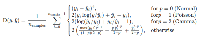
Отклонение от твиди — однородная функция степени 2-power. Таким образом, гамма-распределение power=2 означает, что одновременно масштабируется y_true и y_pred не влияет на отклонение. Для распределения Пуассона power=1 отклонение масштабируется линейно, а для нормального распределения ( power=0) — квадратично. В общем, чем выше, powerтем меньше веса придается крайним отклонениям между истинными и прогнозируемыми целевыми значениями.
Например, давайте сравним два прогноза 1.0 и 100, которые оба составляют 50% от их соответствующего истинного значения.
Среднеквадратичная ошибка ( power=0) очень чувствительна к разнице прогнозов второй точки:
>>> from sklearn.metrics import mean_tweedie_deviance
>>> mean_tweedie_deviance([1.0], [1.5], power=0)
0.25
>>> mean_tweedie_deviance([100.], [150.], power=0)
2500.0
Если увеличить powerдо 1:
>>> mean_tweedie_deviance([1.0], [1.5], power=1)
0.18...
>>> mean_tweedie_deviance([100.], [150.], power=1)
18.9...
разница в ошибках уменьшается. Наконец, установив power=2:
>>> mean_tweedie_deviance([1.0], [1.5], power=2)
0.14...
>>> mean_tweedie_deviance([100.], [150.], power=2)
0.14...
мы получим идентичные ошибки. Таким образом, отклонение when power=2чувствительно только к относительным ошибкам.
3.3.5. Метрики кластеризации
В модуле sklearn.metrics реализованы несколько функций потерь, оценки и полезности. Для получения дополнительной информации см. Раздел « Оценка производительности кластеризации » для кластеризации экземпляров и « Оценка бикластеризации» для бикластеризации.
3.3.6. Фиктивные оценки
При обучении с учителем простая проверка работоспособности состоит из сравнения своей оценки с простыми практическими правилами. DummyClassifier реализует несколько таких простых стратегий классификации:
stratifiedгенерирует случайные прогнозы, соблюдая распределение классов обучающего набора.most_frequentвсегда предсказывает наиболее частую метку в обучающем наборе.priorвсегда предсказывает класс, который максимизирует предыдущий класс (какmost_frequent) иpredict_probaвозвращает предыдущий класс.uniformгенерирует предсказания равномерно в случайном порядке.constantвсегда предсказывает постоянную метку, предоставленную пользователем. Основная мотивация этого метода — оценка F1, когда положительный класс находится в меньшинстве.
Обратите внимание, что со всеми этими стратегиями predict метод полностью игнорирует входные данные!
Для иллюстрации DummyClassifier сначала создадим несбалансированный набор данных:
>>> from sklearn.datasets import load_iris
>>> from sklearn.model_selection import train_test_split
>>> X, y = load_iris(return_X_y=True)
>>> y[y != 1] = -1
>>> X_train, X_test, y_train, y_test = train_test_split(X, y, random_state=0)
Далее сравним точность SVC и most_frequent:
>>> from sklearn.dummy import DummyClassifier
>>> from sklearn.svm import SVC
>>> clf = SVC(kernel='linear', C=1).fit(X_train, y_train)
>>> clf.score(X_test, y_test)
0.63...
>>> clf = DummyClassifier(strategy='most_frequent', random_state=0)
>>> clf.fit(X_train, y_train)
DummyClassifier(random_state=0, strategy='most_frequent')
>>> clf.score(X_test, y_test)
0.57...
Мы видим, что SVC это не намного лучше, чем фиктивный классификатор. Теперь давайте изменим ядро:
>>> clf = SVC(kernel='rbf', C=1).fit(X_train, y_train)
>>> clf.score(X_test, y_test)
0.94...
Мы видим, что точность увеличена почти до 100%. Для лучшей оценки точности рекомендуется стратегия перекрестной проверки, если она не требует слишком больших затрат на ЦП. Для получения дополнительной информации см. Раздел « Перекрестная проверка: оценка производительности оценщика ». Более того, если вы хотите оптимизировать пространство параметров, настоятельно рекомендуется использовать соответствующую методологию; подробности см. в разделе « Настройка гиперпараметров оценщика ».
В более общем плане, когда точность классификатора слишком близка к случайной, это, вероятно, означает, что что-то пошло не так: функции бесполезны, гиперпараметр настроен неправильно, классификатор страдает от дисбаланса классов и т. Д.
DummyRegressor также реализует четыре простых правила регрессии:
meanвсегда предсказывает среднее значение тренировочных целей.medianвсегда предсказывает медианное значение тренировочных целей.quantileвсегда предсказывает предоставленный пользователем квантиль учебных целей.constantвсегда предсказывает постоянное значение, предоставляемое пользователем.
Во всех этих стратегиях predict метод полностью игнорирует входные данные.
.. currentmodule:: sklearn
Metrics and scoring: quantifying the quality of predictions
There are 3 different APIs for evaluating the quality of a model’s
predictions:
- Estimator score method: Estimators have a
scoremethod providing a
default evaluation criterion for the problem they are designed to solve.
This is not discussed on this page, but in each estimator’s documentation. - Scoring parameter: Model-evaluation tools using
:ref:`cross-validation <cross_validation>` (such as
:func:`model_selection.cross_val_score` and
:class:`model_selection.GridSearchCV`) rely on an internal scoring strategy.
This is discussed in the section :ref:`scoring_parameter`. - Metric functions: The :mod:`sklearn.metrics` module implements functions
assessing prediction error for specific purposes. These metrics are detailed
in sections on :ref:`classification_metrics`,
:ref:`multilabel_ranking_metrics`, :ref:`regression_metrics` and
:ref:`clustering_metrics`.
Finally, :ref:`dummy_estimators` are useful to get a baseline
value of those metrics for random predictions.
.. seealso::

   For "pairwise" metrics, between *samples* and not estimators or
   predictions, see the :ref:`metrics` section.
The scoring parameter: defining model evaluation rules
Model selection and evaluation using tools, such as
:class:`model_selection.GridSearchCV` and
:func:`model_selection.cross_val_score`, take a scoring parameter that
controls what metric they apply to the estimators evaluated.
Common cases: predefined values
For the most common use cases, you can designate a scorer object with the
scoring parameter; the table below shows all possible values.
All scorer objects follow the convention that higher return values are better
than lower return values. Thus metrics which measure the distance between
the model and the data, like :func:`metrics.mean_squared_error`, are
available as neg_mean_squared_error which return the negated value
of the metric.
| Scoring | Function | Comment |
|---|---|---|
| Classification | ||
| ‘accuracy’ | :func:`metrics.accuracy_score` | |
| ‘balanced_accuracy’ | :func:`metrics.balanced_accuracy_score` | |
| ‘top_k_accuracy’ | :func:`metrics.top_k_accuracy_score` | |
| ‘average_precision’ | :func:`metrics.average_precision_score` | |
| ‘neg_brier_score’ | :func:`metrics.brier_score_loss` | |
| ‘f1’ | :func:`metrics.f1_score` | for binary targets |
| ‘f1_micro’ | :func:`metrics.f1_score` | micro-averaged |
| ‘f1_macro’ | :func:`metrics.f1_score` | macro-averaged |
| ‘f1_weighted’ | :func:`metrics.f1_score` | weighted average |
| ‘f1_samples’ | :func:`metrics.f1_score` | by multilabel sample |
| ‘neg_log_loss’ | :func:`metrics.log_loss` | requires predict_proba support |
| ‘precision’ etc. | :func:`metrics.precision_score` | suffixes apply as with ‘f1’ |
| ‘recall’ etc. | :func:`metrics.recall_score` | suffixes apply as with ‘f1’ |
| ‘jaccard’ etc. | :func:`metrics.jaccard_score` | suffixes apply as with ‘f1’ |
| ‘roc_auc’ | :func:`metrics.roc_auc_score` | |
| ‘roc_auc_ovr’ | :func:`metrics.roc_auc_score` | |
| ‘roc_auc_ovo’ | :func:`metrics.roc_auc_score` | |
| ‘roc_auc_ovr_weighted’ | :func:`metrics.roc_auc_score` | |
| ‘roc_auc_ovo_weighted’ | :func:`metrics.roc_auc_score` | |
| Clustering | ||
| ‘adjusted_mutual_info_score’ | :func:`metrics.adjusted_mutual_info_score` | |
| ‘adjusted_rand_score’ | :func:`metrics.adjusted_rand_score` | |
| ‘completeness_score’ | :func:`metrics.completeness_score` | |
| ‘fowlkes_mallows_score’ | :func:`metrics.fowlkes_mallows_score` | |
| ‘homogeneity_score’ | :func:`metrics.homogeneity_score` | |
| ‘mutual_info_score’ | :func:`metrics.mutual_info_score` | |
| ‘normalized_mutual_info_score’ | :func:`metrics.normalized_mutual_info_score` | |
| ‘rand_score’ | :func:`metrics.rand_score` | |
| ‘v_measure_score’ | :func:`metrics.v_measure_score` | |
| Regression | ||
| ‘explained_variance’ | :func:`metrics.explained_variance_score` | |
| ‘max_error’ | :func:`metrics.max_error` | |
| ‘neg_mean_absolute_error’ | :func:`metrics.mean_absolute_error` | |
| ‘neg_mean_squared_error’ | :func:`metrics.mean_squared_error` | |
| ‘neg_root_mean_squared_error’ | :func:`metrics.mean_squared_error` | |
| ‘neg_mean_squared_log_error’ | :func:`metrics.mean_squared_log_error` | |
| ‘neg_median_absolute_error’ | :func:`metrics.median_absolute_error` | |
| ‘r2’ | :func:`metrics.r2_score` | |
| ‘neg_mean_poisson_deviance’ | :func:`metrics.mean_poisson_deviance` | |
| ‘neg_mean_gamma_deviance’ | :func:`metrics.mean_gamma_deviance` | |
| ‘neg_mean_absolute_percentage_error’ | :func:`metrics.mean_absolute_percentage_error` | |
| ‘d2_absolute_error_score’ | :func:`metrics.d2_absolute_error_score` | |
| ‘d2_pinball_score’ | :func:`metrics.d2_pinball_score` | |
| ‘d2_tweedie_score’ | :func:`metrics.d2_tweedie_score` |
Usage examples:
>>> from sklearn import svm, datasets
>>> from sklearn.model_selection import cross_val_score
>>> X, y = datasets.load_iris(return_X_y=True)
>>> clf = svm.SVC(random_state=0)
>>> cross_val_score(clf, X, y, cv=5, scoring='recall_macro')
array([0.96..., 0.96..., 0.96..., 0.93..., 1.        ])
>>> model = svm.SVC()
>>> cross_val_score(model, X, y, cv=5, scoring='wrong_choice')
Traceback (most recent call last):
ValueError: 'wrong_choice' is not a valid scoring value. Use
sklearn.metrics.get_scorer_names() to get valid options.
Note
The values listed by the ValueError exception correspond to the
functions measuring prediction accuracy described in the following
sections. You can retrieve the names of all available scorers by calling
:func:`~sklearn.metrics.get_scorer_names`.
.. currentmodule:: sklearn.metrics
Defining your scoring strategy from metric functions
The module :mod:`sklearn.metrics` also exposes a set of simple functions
measuring a prediction error given ground truth and prediction:
- functions ending with
_scorereturn a value to
maximize, the higher the better. - functions ending with
_erroror_lossreturn a
value to minimize, the lower the better. When converting
into a scorer object using :func:`make_scorer`, set
thegreater_is_betterparameter toFalse(Trueby default; see the
parameter description below).
Metrics available for various machine learning tasks are detailed in sections
below.
Many metrics are not given names to be used as scoring values,
sometimes because they require additional parameters, such as
:func:`fbeta_score`. In such cases, you need to generate an appropriate
scoring object. The simplest way to generate a callable object for scoring
is by using :func:`make_scorer`. That function converts metrics
into callables that can be used for model evaluation.
One typical use case is to wrap an existing metric function from the library
with non-default values for its parameters, such as the beta parameter for
the :func:`fbeta_score` function:
>>> from sklearn.metrics import fbeta_score, make_scorer
>>> ftwo_scorer = make_scorer(fbeta_score, beta=2)
>>> from sklearn.model_selection import GridSearchCV
>>> from sklearn.svm import LinearSVC
>>> grid = GridSearchCV(LinearSVC(), param_grid={'C': [1, 10]},
...                     scoring=ftwo_scorer, cv=5)
The second use case is to build a completely custom scorer object
from a simple python function using :func:`make_scorer`, which can
take several parameters:
- the python function you want to use (
my_custom_loss_func
in the example below) - whether the python function returns a score (
greater_is_better=True,
the default) or a loss (greater_is_better=False). If a loss, the output
of the python function is negated by the scorer object, conforming to
the cross validation convention that scorers return higher values for better models. - for classification metrics only: whether the python function you provided requires continuous decision
certainties (needs_threshold=True). The default value is
False. - any additional parameters, such as
betaorlabelsin :func:`f1_score`.
Here is an example of building custom scorers, and of using the
greater_is_better parameter:
>>> import numpy as np
>>> def my_custom_loss_func(y_true, y_pred):
...     diff = np.abs(y_true - y_pred).max()
...     return np.log1p(diff)
...
>>> # score will negate the return value of my_custom_loss_func,
>>> # which will be np.log(2), 0.693, given the values for X
>>> # and y defined below.
>>> score = make_scorer(my_custom_loss_func, greater_is_better=False)
>>> X = [[1], [1]]
>>> y = [0, 1]
>>> from sklearn.dummy import DummyClassifier
>>> clf = DummyClassifier(strategy='most_frequent', random_state=0)
>>> clf = clf.fit(X, y)
>>> my_custom_loss_func(y, clf.predict(X))
0.69...
>>> score(clf, X, y)
-0.69...
Implementing your own scoring object
You can generate even more flexible model scorers by constructing your own
scoring object from scratch, without using the :func:`make_scorer` factory.
For a callable to be a scorer, it needs to meet the protocol specified by
the following two rules:
- It can be called with parameters
(estimator, X, y), whereestimator
is the model that should be evaluated,Xis validation data, andyis
the ground truth target forX(in the supervised case) orNone(in the
unsupervised case). - It returns a floating point number that quantifies the
estimatorprediction quality onX, with reference toy.
Again, by convention higher numbers are better, so if your scorer
returns loss, that value should be negated.
Note
Using custom scorers in functions where n_jobs > 1
While defining the custom scoring function alongside the calling function
should work out of the box with the default joblib backend (loky),
importing it from another module will be a more robust approach and work
independently of the joblib backend.
For example, to use n_jobs greater than 1 in the example below,
custom_scoring_function function is saved in a user-created module
(custom_scorer_module.py) and imported:
>>> from custom_scorer_module import custom_scoring_function # doctest: +SKIP
>>> cross_val_score(model,
...  X_train,
...  y_train,
...  scoring=make_scorer(custom_scoring_function, greater_is_better=False),
...  cv=5,
...  n_jobs=-1) # doctest: +SKIP
Using multiple metric evaluation
Scikit-learn also permits evaluation of multiple metrics in GridSearchCV,
RandomizedSearchCV and cross_validate.
There are three ways to specify multiple scoring metrics for the scoring
parameter:
-
- As an iterable of string metrics::
-
>>> scoring = ['accuracy', 'precision']
-
- As a
dictmapping the scorer name to the scoring function:: -
>>> from sklearn.metrics import accuracy_score
>>> from sklearn.metrics import make_scorer
>>> scoring = {'accuracy': make_scorer(accuracy_score),
...            'prec': 'precision'}
Note that the dict values can either be scorer functions or one of the
predefined metric strings. - As a
-
As a callable that returns a dictionary of scores:
>>> from sklearn.model_selection import cross_validate
>>> from sklearn.metrics import confusion_matrix
>>> # A sample toy binary classification dataset
>>> X, y = datasets.make_classification(n_classes=2, random_state=0)
>>> svm = LinearSVC(random_state=0)
>>> def confusion_matrix_scorer(clf, X, y):
...      y_pred = clf.predict(X)
...      cm = confusion_matrix(y, y_pred)
...      return {'tn': cm[0, 0], 'fp': cm[0, 1],
...              'fn': cm[1, 0], 'tp': cm[1, 1]}
>>> cv_results = cross_validate(svm, X, y, cv=5,
...                             scoring=confusion_matrix_scorer)
>>> # Getting the test set true positive scores
>>> print(cv_results['test_tp'])
[10  9  8  7  8]
>>> # Getting the test set false negative scores
>>> print(cv_results['test_fn'])
[0 1 2 3 2]
Classification metrics
.. currentmodule:: sklearn.metrics
The :mod:`sklearn.metrics` module implements several loss, score, and utility
functions to measure classification performance.
Some metrics might require probability estimates of the positive class,
confidence values, or binary decisions values.
Most implementations allow each sample to provide a weighted contribution
to the overall score, through the sample_weight parameter.
Some of these are restricted to the binary classification case:
.. autosummary::

   precision_recall_curve
   roc_curve
   class_likelihood_ratios
   det_curve
Others also work in the multiclass case:
.. autosummary::

   balanced_accuracy_score
   cohen_kappa_score
   confusion_matrix
   hinge_loss
   matthews_corrcoef
   roc_auc_score
   top_k_accuracy_score
Some also work in the multilabel case:
.. autosummary::

   accuracy_score
   classification_report
   f1_score
   fbeta_score
   hamming_loss
   jaccard_score
   log_loss
   multilabel_confusion_matrix
   precision_recall_fscore_support
   precision_score
   recall_score
   roc_auc_score
   zero_one_loss
And some work with binary and multilabel (but not multiclass) problems:
.. autosummary::

   average_precision_score
In the following sub-sections, we will describe each of those functions,
preceded by some notes on common API and metric definition.
From binary to multiclass and multilabel
Some metrics are essentially defined for binary classification tasks (e.g.
:func:`f1_score`, :func:`roc_auc_score`). In these cases, by default
only the positive label is evaluated, assuming by default that the positive
class is labelled 1 (though this may be configurable through the
pos_label parameter).
In extending a binary metric to multiclass or multilabel problems, the data
is treated as a collection of binary problems, one for each class.
There are then a number of ways to average binary metric calculations across
the set of classes, each of which may be useful in some scenario.
Where available, you should select among these using the average parameter.
"macro"simply calculates the mean of the binary metrics,
giving equal weight to each class. In problems where infrequent classes
are nonetheless important, macro-averaging may be a means of highlighting
their performance. On the other hand, the assumption that all classes are
equally important is often untrue, such that macro-averaging will
over-emphasize the typically low performance on an infrequent class."weighted"accounts for class imbalance by computing the average of
binary metrics in which each class’s score is weighted by its presence in the
true data sample."micro"gives each sample-class pair an equal contribution to the overall
metric (except as a result of sample-weight). Rather than summing the
metric per class, this sums the dividends and divisors that make up the
per-class metrics to calculate an overall quotient.
Micro-averaging may be preferred in multilabel settings, including
multiclass classification where a majority class is to be ignored."samples"applies only to multilabel problems. It does not calculate a
per-class measure, instead calculating the metric over the true and predicted
classes for each sample in the evaluation data, and returning their
(sample_weight-weighted) average.- Selecting
average=Nonewill return an array with the score for each
class.
While multiclass data is provided to the metric, like binary targets, as an
array of class labels, multilabel data is specified as an indicator matrix,
in which cell [i, j] has value 1 if sample i has label j and value
0 otherwise.
Accuracy score
The :func:`accuracy_score` function computes the
accuracy, either the fraction
(default) or the count (normalize=False) of correct predictions.
In multilabel classification, the function returns the subset accuracy. If
the entire set of predicted labels for a sample strictly match with the true
set of labels, then the subset accuracy is 1.0; otherwise it is 0.0.
If hat{y}_i is the predicted value of
the i-th sample and y_i is the corresponding true value,
then the fraction of correct predictions over n_text{samples} is
defined as
texttt{accuracy}(y, hat{y}) = frac{1}{n_text{samples}} sum_{i=0}^{n_text{samples}-1} 1(hat{y}_i = y_i)
where 1(x) is the indicator function.
>>> import numpy as np
>>> from sklearn.metrics import accuracy_score
>>> y_pred = [0, 2, 1, 3]
>>> y_true = [0, 1, 2, 3]
>>> accuracy_score(y_true, y_pred)
0.5
>>> accuracy_score(y_true, y_pred, normalize=False)
2
In the multilabel case with binary label indicators:
>>> accuracy_score(np.array([[0, 1], [1, 1]]), np.ones((2, 2)))
0.5
Example:
- See :ref:`sphx_glr_auto_examples_model_selection_plot_permutation_tests_for_classification.py`
for an example of accuracy score usage using permutations of
the dataset.
Top-k accuracy score
The :func:`top_k_accuracy_score` function is a generalization of
:func:`accuracy_score`. The difference is that a prediction is considered
correct as long as the true label is associated with one of the k highest
predicted scores. :func:`accuracy_score` is the special case of k = 1.
The function covers the binary and multiclass classification cases but not the
multilabel case.
If hat{f}_{i,j} is the predicted class for the i-th sample
corresponding to the j-th largest predicted score and y_i is the
corresponding true value, then the fraction of correct predictions over
n_text{samples} is defined as
texttt{top-k accuracy}(y, hat{f}) = frac{1}{n_text{samples}} sum_{i=0}^{n_text{samples}-1} sum_{j=1}^{k} 1(hat{f}_{i,j} = y_i)
where k is the number of guesses allowed and 1(x) is the
indicator function.
>>> import numpy as np
>>> from sklearn.metrics import top_k_accuracy_score
>>> y_true = np.array([0, 1, 2, 2])
>>> y_score = np.array([[0.5, 0.2, 0.2],
...                     [0.3, 0.4, 0.2],
...                     [0.2, 0.4, 0.3],
...                     [0.7, 0.2, 0.1]])
>>> top_k_accuracy_score(y_true, y_score, k=2)
0.75
>>> # Not normalizing gives the number of "correctly" classified samples
>>> top_k_accuracy_score(y_true, y_score, k=2, normalize=False)
3
Balanced accuracy score
The :func:`balanced_accuracy_score` function computes the balanced accuracy, which avoids inflated
performance estimates on imbalanced datasets. It is the macro-average of recall
scores per class or, equivalently, raw accuracy where each sample is weighted
according to the inverse prevalence of its true class.
Thus for balanced datasets, the score is equal to accuracy.
In the binary case, balanced accuracy is equal to the arithmetic mean of
sensitivity
(true positive rate) and specificity (true negative
rate), or the area under the ROC curve with binary predictions rather than
scores:
texttt{balanced-accuracy} = frac{1}{2}left( frac{TP}{TP + FN} + frac{TN}{TN + FP}right )
If the classifier performs equally well on either class, this term reduces to
the conventional accuracy (i.e., the number of correct predictions divided by
the total number of predictions).
In contrast, if the conventional accuracy is above chance only because the
classifier takes advantage of an imbalanced test set, then the balanced
accuracy, as appropriate, will drop to frac{1}{n_classes}.
The score ranges from 0 to 1, or when adjusted=True is used, it rescaled to
the range frac{1}{1 — n_classes} to 1, inclusive, with
performance at random scoring 0.
If y_i is the true value of the i-th sample, and w_i
is the corresponding sample weight, then we adjust the sample weight to:
hat{w}_i = frac{w_i}{sum_j{1(y_j = y_i) w_j}}
where 1(x) is the indicator function.
Given predicted hat{y}_i for sample i, balanced accuracy is
defined as:
texttt{balanced-accuracy}(y, hat{y}, w) = frac{1}{sum{hat{w}_i}} sum_i 1(hat{y}_i = y_i) hat{w}_i
With adjusted=True, balanced accuracy reports the relative increase from
texttt{balanced-accuracy}(y, mathbf{0}, w) =
frac{1}{n_classes}. In the binary case, this is also known as
*Youden’s J statistic*,
or informedness.
Note
The multiclass definition here seems the most reasonable extension of the
metric used in binary classification, though there is no certain consensus
in the literature:
- Our definition: [Mosley2013], [Kelleher2015] and [Guyon2015], where
[Guyon2015] adopt the adjusted version to ensure that random predictions
have a score of 0 and perfect predictions have a score of 1.. - Class balanced accuracy as described in [Mosley2013]: the minimum between the precision
and the recall for each class is computed. Those values are then averaged over the total
number of classes to get the balanced accuracy. - Balanced Accuracy as described in [Urbanowicz2015]: the average of sensitivity and specificity
is computed for each class and then averaged over total number of classes.
References:
| [Guyon2015] | (1, 2) I. Guyon, K. Bennett, G. Cawley, H.J. Escalante, S. Escalera, T.K. Ho, N. Macià, B. Ray, M. Saeed, A.R. Statnikov, E. Viegas, Design of the 2015 ChaLearn AutoML Challenge, IJCNN 2015. |
| [Urbanowicz2015] | Urbanowicz R.J., Moore, J.H. :doi:`ExSTraCS 2.0: description and evaluation of a scalable learning classifier system <10.1007/s12065-015-0128-8>`, Evol. Intel. (2015) 8: 89. |
Cohen’s kappa
The function :func:`cohen_kappa_score` computes Cohen’s kappa statistic.
This measure is intended to compare labelings by different human annotators,
not a classifier versus a ground truth.
The kappa score (see docstring) is a number between -1 and 1.
Scores above .8 are generally considered good agreement;
zero or lower means no agreement (practically random labels).
Kappa scores can be computed for binary or multiclass problems,
but not for multilabel problems (except by manually computing a per-label score)
and not for more than two annotators.
>>> from sklearn.metrics import cohen_kappa_score
>>> y_true = [2, 0, 2, 2, 0, 1]
>>> y_pred = [0, 0, 2, 2, 0, 2]
>>> cohen_kappa_score(y_true, y_pred)
0.4285714285714286
Confusion matrix
The :func:`confusion_matrix` function evaluates
classification accuracy by computing the confusion matrix with each row corresponding
to the true class (Wikipedia and other references may use different convention
for axes).
By definition, entry i, j in a confusion matrix is
the number of observations actually in group i, but
predicted to be in group j. Here is an example:
>>> from sklearn.metrics import confusion_matrix
>>> y_true = [2, 0, 2, 2, 0, 1]
>>> y_pred = [0, 0, 2, 2, 0, 2]
>>> confusion_matrix(y_true, y_pred)
array([[2, 0, 0],
       [0, 0, 1],
       [1, 0, 2]])
:class:`ConfusionMatrixDisplay` can be used to visually represent a confusion
matrix as shown in the
:ref:`sphx_glr_auto_examples_model_selection_plot_confusion_matrix.py`
example, which creates the following figure:

The parameter normalize allows to report ratios instead of counts. The
confusion matrix can be normalized in 3 different ways: 'pred', 'true',
and 'all' which will divide the counts by the sum of each columns, rows, or
the entire matrix, respectively.
>>> y_true = [0, 0, 0, 1, 1, 1, 1, 1]
>>> y_pred = [0, 1, 0, 1, 0, 1, 0, 1]
>>> confusion_matrix(y_true, y_pred, normalize='all')
array([[0.25 , 0.125],
       [0.25 , 0.375]])
For binary problems, we can get counts of true negatives, false positives,
false negatives and true positives as follows:
>>> y_true = [0, 0, 0, 1, 1, 1, 1, 1]
>>> y_pred = [0, 1, 0, 1, 0, 1, 0, 1]
>>> tn, fp, fn, tp = confusion_matrix(y_true, y_pred).ravel()
>>> tn, fp, fn, tp
(2, 1, 2, 3)
Example:
- See :ref:`sphx_glr_auto_examples_model_selection_plot_confusion_matrix.py`
for an example of using a confusion matrix to evaluate classifier output
quality. - See :ref:`sphx_glr_auto_examples_classification_plot_digits_classification.py`
for an example of using a confusion matrix to classify
hand-written digits. - See :ref:`sphx_glr_auto_examples_text_plot_document_classification_20newsgroups.py`
for an example of using a confusion matrix to classify text
documents.
Classification report
The :func:`classification_report` function builds a text report showing the
main classification metrics. Here is a small example with custom target_names
and inferred labels:
>>> from sklearn.metrics import classification_report
>>> y_true = [0, 1, 2, 2, 0]
>>> y_pred = [0, 0, 2, 1, 0]
>>> target_names = ['class 0', 'class 1', 'class 2']
>>> print(classification_report(y_true, y_pred, target_names=target_names))
              precision    recall  f1-score   support
<BLANKLINE>
     class 0       0.67      1.00      0.80         2
     class 1       0.00      0.00      0.00         1
     class 2       1.00      0.50      0.67         2
<BLANKLINE>
    accuracy                           0.60         5
   macro avg       0.56      0.50      0.49         5
weighted avg       0.67      0.60      0.59         5
<BLANKLINE>
Example:
- See :ref:`sphx_glr_auto_examples_classification_plot_digits_classification.py`
for an example of classification report usage for
hand-written digits. - See :ref:`sphx_glr_auto_examples_model_selection_plot_grid_search_digits.py`
for an example of classification report usage for
grid search with nested cross-validation.
Hamming loss
The :func:`hamming_loss` computes the average Hamming loss or Hamming
distance between two sets
of samples.
If hat{y}_{i,j} is the predicted value for the j-th label of a
given sample i, y_{i,j} is the corresponding true value,
n_text{samples} is the number of samples and n_text{labels}
is the number of labels, then the Hamming loss L_{Hamming} is defined
as:
L_{Hamming}(y, hat{y}) = frac{1}{n_text{samples} * n_text{labels}} sum_{i=0}^{n_text{samples}-1} sum_{j=0}^{n_text{labels} - 1} 1(hat{y}_{i,j} not= y_{i,j})
where 1(x) is the indicator function.
The equation above does not hold true in the case of multiclass classification.
Please refer to the note below for more information.
>>> from sklearn.metrics import hamming_loss
>>> y_pred = [1, 2, 3, 4]
>>> y_true = [2, 2, 3, 4]
>>> hamming_loss(y_true, y_pred)
0.25
In the multilabel case with binary label indicators:
>>> hamming_loss(np.array([[0, 1], [1, 1]]), np.zeros((2, 2)))
0.75
Note
In multiclass classification, the Hamming loss corresponds to the Hamming
distance between y_true and y_pred which is similar to the
:ref:`zero_one_loss` function. However, while zero-one loss penalizes
prediction sets that do not strictly match true sets, the Hamming loss
penalizes individual labels. Thus the Hamming loss, upper bounded by the zero-one
loss, is always between zero and one, inclusive; and predicting a proper subset
or superset of the true labels will give a Hamming loss between
zero and one, exclusive.
Precision, recall and F-measures
Intuitively, precision is the ability
of the classifier not to label as positive a sample that is negative, and
recall is the
ability of the classifier to find all the positive samples.
The F-measure
(F_beta and F_1 measures) can be interpreted as a weighted
harmonic mean of the precision and recall. A
F_beta measure reaches its best value at 1 and its worst score at 0.
With beta = 1, F_beta and
F_1 are equivalent, and the recall and the precision are equally important.
The :func:`precision_recall_curve` computes a precision-recall curve
from the ground truth label and a score given by the classifier
by varying a decision threshold.
The :func:`average_precision_score` function computes the
average precision
(AP) from prediction scores. The value is between 0 and 1 and higher is better.
AP is defined as
text{AP} = sum_n (R_n - R_{n-1}) P_n
where P_n and R_n are the precision and recall at the
nth threshold. With random predictions, the AP is the fraction of positive
samples.
References [Manning2008] and [Everingham2010] present alternative variants of
AP that interpolate the precision-recall curve. Currently,
:func:`average_precision_score` does not implement any interpolated variant.
References [Davis2006] and [Flach2015] describe why a linear interpolation of
points on the precision-recall curve provides an overly-optimistic measure of
classifier performance. This linear interpolation is used when computing area
under the curve with the trapezoidal rule in :func:`auc`.
Several functions allow you to analyze the precision, recall and F-measures
score:
.. autosummary::

   average_precision_score
   f1_score
   fbeta_score
   precision_recall_curve
   precision_recall_fscore_support
   precision_score
   recall_score
Note that the :func:`precision_recall_curve` function is restricted to the
binary case. The :func:`average_precision_score` function works only in
binary classification and multilabel indicator format.
The :func:`PredictionRecallDisplay.from_estimator` and
:func:`PredictionRecallDisplay.from_predictions` functions will plot the
precision-recall curve as follows.

Examples:
- See :ref:`sphx_glr_auto_examples_model_selection_plot_grid_search_digits.py`
for an example of :func:`precision_score` and :func:`recall_score` usage
to estimate parameters using grid search with nested cross-validation. - See :ref:`sphx_glr_auto_examples_model_selection_plot_precision_recall.py`
for an example of :func:`precision_recall_curve` usage to evaluate
classifier output quality.
References:
| [Manning2008] | C.D. Manning, P. Raghavan, H. Schütze, Introduction to Information Retrieval, 2008. |
| [Everingham2010] | M. Everingham, L. Van Gool, C.K.I. Williams, J. Winn, A. Zisserman, The Pascal Visual Object Classes (VOC) Challenge, IJCV 2010. |
Binary classification
In a binary classification task, the terms »positive» and »negative» refer
to the classifier’s prediction, and the terms »true» and »false» refer to
whether that prediction corresponds to the external judgment (sometimes known
as the »observation»). Given these definitions, we can formulate the
following table:
| Actual class (observation) | ||
| Predicted class (expectation) |
tp (true positive) Correct result |
fp (false positive) Unexpected result |
| fn (false negative) Missing result |
tn (true negative) Correct absence of result |
In this context, we can define the notions of precision, recall and F-measure:
text{precision} = frac{tp}{tp + fp},
text{recall} = frac{tp}{tp + fn},
F_beta = (1 + beta^2) frac{text{precision} times text{recall}}{beta^2 text{precision} + text{recall}}.
Sometimes recall is also called »sensitivity».
Here are some small examples in binary classification:
>>> from sklearn import metrics
>>> y_pred = [0, 1, 0, 0]
>>> y_true = [0, 1, 0, 1]
>>> metrics.precision_score(y_true, y_pred)
1.0
>>> metrics.recall_score(y_true, y_pred)
0.5
>>> metrics.f1_score(y_true, y_pred)
0.66...
>>> metrics.fbeta_score(y_true, y_pred, beta=0.5)
0.83...
>>> metrics.fbeta_score(y_true, y_pred, beta=1)
0.66...
>>> metrics.fbeta_score(y_true, y_pred, beta=2)
0.55...
>>> metrics.precision_recall_fscore_support(y_true, y_pred, beta=0.5)
(array([0.66..., 1.        ]), array([1. , 0.5]), array([0.71..., 0.83...]), array([2, 2]))


>>> import numpy as np
>>> from sklearn.metrics import precision_recall_curve
>>> from sklearn.metrics import average_precision_score
>>> y_true = np.array([0, 0, 1, 1])
>>> y_scores = np.array([0.1, 0.4, 0.35, 0.8])
>>> precision, recall, threshold = precision_recall_curve(y_true, y_scores)
>>> precision
array([0.5       , 0.66..., 0.5       , 1.        , 1.        ])
>>> recall
array([1. , 1. , 0.5, 0.5, 0. ])
>>> threshold
array([0.1 , 0.35, 0.4 , 0.8 ])
>>> average_precision_score(y_true, y_scores)
0.83...
Multiclass and multilabel classification
In a multiclass and multilabel classification task, the notions of precision,
recall, and F-measures can be applied to each label independently.
There are a few ways to combine results across labels,
specified by the average argument to the
:func:`average_precision_score` (multilabel only), :func:`f1_score`,
:func:`fbeta_score`, :func:`precision_recall_fscore_support`,
:func:`precision_score` and :func:`recall_score` functions, as described
:ref:`above <average>`. Note that if all labels are included, «micro»-averaging
in a multiclass setting will produce precision, recall and F
that are all identical to accuracy. Also note that «weighted» averaging may
produce an F-score that is not between precision and recall.
To make this more explicit, consider the following notation:
- y the set of true (sample, label) pairs
- hat{y} the set of predicted (sample, label) pairs
- L the set of labels
- S the set of samples
- y_s the subset of y with sample s,
i.e. y_s := left{(s’, l) in y | s’ = sright} - y_l the subset of y with label l
- similarly, hat{y}_s and hat{y}_l are subsets of
hat{y} - P(A, B) := frac{left| A cap B right|}{left|Bright|} for some
sets A and B - R(A, B) := frac{left| A cap B right|}{left|Aright|}
(Conventions vary on handling A = emptyset; this implementation uses
R(A, B):=0, and similar for P.) - F_beta(A, B) := left(1 + beta^2right) frac{P(A, B) times R(A, B)}{beta^2 P(A, B) + R(A, B)}
Then the metrics are defined as:
average |
Precision | Recall | F_beta |
|---|---|---|---|
"micro" |
P(y, hat{y}) | R(y, hat{y}) | F_beta(y, hat{y}) |
"samples" |
frac{1}{left|Sright|} sum_{s in S} P(y_s, hat{y}_s) | frac{1}{left|Sright|} sum_{s in S} R(y_s, hat{y}_s) | frac{1}{left|Sright|} sum_{s in S} F_beta(y_s, hat{y}_s) |
"macro" |
frac{1}{left|Lright|} sum_{l in L} P(y_l, hat{y}_l) | frac{1}{left|Lright|} sum_{l in L} R(y_l, hat{y}_l) | frac{1}{left|Lright|} sum_{l in L} F_beta(y_l, hat{y}_l) |
"weighted" |
frac{1}{sum_{l in L} left|y_lright|} sum_{l in L} left|y_lright| P(y_l, hat{y}_l) | frac{1}{sum_{l in L} left|y_lright|} sum_{l in L} left|y_lright| R(y_l, hat{y}_l) | frac{1}{sum_{l in L} left|y_lright|} sum_{l in L} left|y_lright| F_beta(y_l, hat{y}_l) |
None |
langle P(y_l, hat{y}_l) | l in L rangle | langle R(y_l, hat{y}_l) | l in L rangle | langle F_beta(y_l, hat{y}_l) | l in L rangle |
>>> from sklearn import metrics
>>> y_true = [0, 1, 2, 0, 1, 2]
>>> y_pred = [0, 2, 1, 0, 0, 1]
>>> metrics.precision_score(y_true, y_pred, average='macro')
0.22...
>>> metrics.recall_score(y_true, y_pred, average='micro')
0.33...
>>> metrics.f1_score(y_true, y_pred, average='weighted')
0.26...
>>> metrics.fbeta_score(y_true, y_pred, average='macro', beta=0.5)
0.23...
>>> metrics.precision_recall_fscore_support(y_true, y_pred, beta=0.5, average=None)
(array([0.66..., 0.        , 0.        ]), array([1., 0., 0.]), array([0.71..., 0.        , 0.        ]), array([2, 2, 2]...))
For multiclass classification with a «negative class», it is possible to exclude some labels:
>>> metrics.recall_score(y_true, y_pred, labels=[1, 2], average='micro')
... # excluding 0, no labels were correctly recalled
0.0
Similarly, labels not present in the data sample may be accounted for in macro-averaging.
>>> metrics.precision_score(y_true, y_pred, labels=[0, 1, 2, 3], average='macro')
0.166...
Jaccard similarity coefficient score
The :func:`jaccard_score` function computes the average of Jaccard similarity
coefficients, also called the
Jaccard index, between pairs of label sets.
The Jaccard similarity coefficient with a ground truth label set y and
predicted label set hat{y}, is defined as
J(y, hat{y}) = frac{|y cap hat{y}|}{|y cup hat{y}|}.
The :func:`jaccard_score` (like :func:`precision_recall_fscore_support`) applies
natively to binary targets. By computing it set-wise it can be extended to apply
to multilabel and multiclass through the use of average (see
:ref:`above <average>`).
In the binary case:
>>> import numpy as np
>>> from sklearn.metrics import jaccard_score
>>> y_true = np.array([[0, 1, 1],
...                    [1, 1, 0]])
>>> y_pred = np.array([[1, 1, 1],
...                    [1, 0, 0]])
>>> jaccard_score(y_true[0], y_pred[0])
0.6666...
In the 2D comparison case (e.g. image similarity):
>>> jaccard_score(y_true, y_pred, average="micro")
0.6
In the multilabel case with binary label indicators:
>>> jaccard_score(y_true, y_pred, average='samples')
0.5833...
>>> jaccard_score(y_true, y_pred, average='macro')
0.6666...
>>> jaccard_score(y_true, y_pred, average=None)
array([0.5, 0.5, 1. ])
Multiclass problems are binarized and treated like the corresponding
multilabel problem:
>>> y_pred = [0, 2, 1, 2]
>>> y_true = [0, 1, 2, 2]
>>> jaccard_score(y_true, y_pred, average=None)
array([1. , 0. , 0.33...])
>>> jaccard_score(y_true, y_pred, average='macro')
0.44...
>>> jaccard_score(y_true, y_pred, average='micro')
0.33...
Hinge loss
The :func:`hinge_loss` function computes the average distance between
the model and the data using
hinge loss, a one-sided metric
that considers only prediction errors. (Hinge
loss is used in maximal margin classifiers such as support vector machines.)
If the true label y_i of a binary classification task is encoded as
y_i=left{-1, +1right} for every sample i; and w_i
is the corresponding predicted decision (an array of shape (n_samples,) as
output by the decision_function method), then the hinge loss is defined as:
L_text{Hinge}(y, w) = frac{1}{n_text{samples}} sum_{i=0}^{n_text{samples}-1} maxleft{1 - w_i y_i, 0right}
If there are more than two labels, :func:`hinge_loss` uses a multiclass variant
due to Crammer & Singer.
Here is
the paper describing it.
In this case the predicted decision is an array of shape (n_samples,
n_labels). If w_{i, y_i} is the predicted decision for the true label
y_i of the i-th sample; and
hat{w}_{i, y_i} = maxleft{w_{i, y_j}~|~y_j ne y_i right}
is the maximum of the
predicted decisions for all the other labels, then the multi-class hinge loss
is defined by:
L_text{Hinge}(y, w) = frac{1}{n_text{samples}}
sum_{i=0}^{n_text{samples}-1} maxleft{1 + hat{w}_{i, y_i}
- w_{i, y_i}, 0right}
Here is a small example demonstrating the use of the :func:`hinge_loss` function
with a svm classifier in a binary class problem:
>>> from sklearn import svm
>>> from sklearn.metrics import hinge_loss
>>> X = [[0], [1]]
>>> y = [-1, 1]
>>> est = svm.LinearSVC(random_state=0)
>>> est.fit(X, y)
LinearSVC(random_state=0)
>>> pred_decision = est.decision_function([[-2], [3], [0.5]])
>>> pred_decision
array([-2.18...,  2.36...,  0.09...])
>>> hinge_loss([-1, 1, 1], pred_decision)
0.3...
Here is an example demonstrating the use of the :func:`hinge_loss` function
with a svm classifier in a multiclass problem:
>>> X = np.array([[0], [1], [2], [3]])
>>> Y = np.array([0, 1, 2, 3])
>>> labels = np.array([0, 1, 2, 3])
>>> est = svm.LinearSVC()
>>> est.fit(X, Y)
LinearSVC()
>>> pred_decision = est.decision_function([[-1], [2], [3]])
>>> y_true = [0, 2, 3]
>>> hinge_loss(y_true, pred_decision, labels=labels)
0.56...
Log loss
Log loss, also called logistic regression loss or
cross-entropy loss, is defined on probability estimates. It is
commonly used in (multinomial) logistic regression and neural networks, as well
as in some variants of expectation-maximization, and can be used to evaluate the
probability outputs (predict_proba) of a classifier instead of its
discrete predictions.
For binary classification with a true label y in {0,1}
and a probability estimate p = operatorname{Pr}(y = 1),
the log loss per sample is the negative log-likelihood
of the classifier given the true label:
L_{log}(y, p) = -log operatorname{Pr}(y|p) = -(y log (p) + (1 - y) log (1 - p))
This extends to the multiclass case as follows.
Let the true labels for a set of samples
be encoded as a 1-of-K binary indicator matrix Y,
i.e., y_{i,k} = 1 if sample i has label k
taken from a set of K labels.
Let P be a matrix of probability estimates,
with p_{i,k} = operatorname{Pr}(y_{i,k} = 1).
Then the log loss of the whole set is
L_{log}(Y, P) = -log operatorname{Pr}(Y|P) = - frac{1}{N} sum_{i=0}^{N-1} sum_{k=0}^{K-1} y_{i,k} log p_{i,k}
To see how this generalizes the binary log loss given above,
note that in the binary case,
p_{i,0} = 1 — p_{i,1} and y_{i,0} = 1 — y_{i,1},
so expanding the inner sum over y_{i,k} in {0,1}
gives the binary log loss.
The :func:`log_loss` function computes log loss given a list of ground-truth
labels and a probability matrix, as returned by an estimator’s predict_proba
method.
>>> from sklearn.metrics import log_loss
>>> y_true = [0, 0, 1, 1]
>>> y_pred = [[.9, .1], [.8, .2], [.3, .7], [.01, .99]]
>>> log_loss(y_true, y_pred)
0.1738...
The first [.9, .1] in y_pred denotes 90% probability that the first
sample has label 0. The log loss is non-negative.
Matthews correlation coefficient
The :func:`matthews_corrcoef` function computes the
Matthew’s correlation coefficient (MCC)
for binary classes. Quoting Wikipedia:
«The Matthews correlation coefficient is used in machine learning as a
measure of the quality of binary (two-class) classifications. It takes
into account true and false positives and negatives and is generally
regarded as a balanced measure which can be used even if the classes are
of very different sizes. The MCC is in essence a correlation coefficient
value between -1 and +1. A coefficient of +1 represents a perfect
prediction, 0 an average random prediction and -1 an inverse prediction.
The statistic is also known as the phi coefficient.»
In the binary (two-class) case, tp, tn, fp and
fn are respectively the number of true positives, true negatives, false
positives and false negatives, the MCC is defined as
MCC = frac{tp times tn - fp times fn}{sqrt{(tp + fp)(tp + fn)(tn + fp)(tn + fn)}}.
In the multiclass case, the Matthews correlation coefficient can be defined in terms of a
:func:`confusion_matrix` C for K classes. To simplify the
definition consider the following intermediate variables:
- t_k=sum_{i}^{K} C_{ik} the number of times class k truly occurred,
- p_k=sum_{i}^{K} C_{ki} the number of times class k was predicted,
- c=sum_{k}^{K} C_{kk} the total number of samples correctly predicted,
- s=sum_{i}^{K} sum_{j}^{K} C_{ij} the total number of samples.
Then the multiclass MCC is defined as:
MCC = frac{
    c times s - sum_{k}^{K} p_k times t_k
}{sqrt{
    (s^2 - sum_{k}^{K} p_k^2) times
    (s^2 - sum_{k}^{K} t_k^2)
}}
When there are more than two labels, the value of the MCC will no longer range
between -1 and +1. Instead the minimum value will be somewhere between -1 and 0
depending on the number and distribution of ground true labels. The maximum
value is always +1.
Here is a small example illustrating the usage of the :func:`matthews_corrcoef`
function:
>>> from sklearn.metrics import matthews_corrcoef
>>> y_true = [+1, +1, +1, -1]
>>> y_pred = [+1, -1, +1, +1]
>>> matthews_corrcoef(y_true, y_pred)
-0.33...
Multi-label confusion matrix
The :func:`multilabel_confusion_matrix` function computes class-wise (default)
or sample-wise (samplewise=True) multilabel confusion matrix to evaluate
the accuracy of a classification. multilabel_confusion_matrix also treats
multiclass data as if it were multilabel, as this is a transformation commonly
applied to evaluate multiclass problems with binary classification metrics
(such as precision, recall, etc.).
When calculating class-wise multilabel confusion matrix C, the
count of true negatives for class i is C_{i,0,0}, false
negatives is C_{i,1,0}, true positives is C_{i,1,1}
and false positives is C_{i,0,1}.
Here is an example demonstrating the use of the
:func:`multilabel_confusion_matrix` function with
:term:`multilabel indicator matrix` input:
>>> import numpy as np
>>> from sklearn.metrics import multilabel_confusion_matrix
>>> y_true = np.array([[1, 0, 1],
...                    [0, 1, 0]])
>>> y_pred = np.array([[1, 0, 0],
...                    [0, 1, 1]])
>>> multilabel_confusion_matrix(y_true, y_pred)
array([[[1, 0],
        [0, 1]],
<BLANKLINE>
       [[1, 0],
        [0, 1]],
<BLANKLINE>
       [[0, 1],
        [1, 0]]])
Or a confusion matrix can be constructed for each sample’s labels:
>>> multilabel_confusion_matrix(y_true, y_pred, samplewise=True)
array([[[1, 0],
        [1, 1]],
<BLANKLINE>
       [[1, 1],
        [0, 1]]])
Here is an example demonstrating the use of the
:func:`multilabel_confusion_matrix` function with
:term:`multiclass` input:
>>> y_true = ["cat", "ant", "cat", "cat", "ant", "bird"]
>>> y_pred = ["ant", "ant", "cat", "cat", "ant", "cat"]
>>> multilabel_confusion_matrix(y_true, y_pred,
...                             labels=["ant", "bird", "cat"])
array([[[3, 1],
        [0, 2]],
<BLANKLINE>
       [[5, 0],
        [1, 0]],
<BLANKLINE>
       [[2, 1],
        [1, 2]]])
Here are some examples demonstrating the use of the
:func:`multilabel_confusion_matrix` function to calculate recall
(or sensitivity), specificity, fall out and miss rate for each class in a
problem with multilabel indicator matrix input.
Calculating
recall
(also called the true positive rate or the sensitivity) for each class:
>>> y_true = np.array([[0, 0, 1],
...                    [0, 1, 0],
...                    [1, 1, 0]])
>>> y_pred = np.array([[0, 1, 0],
...                    [0, 0, 1],
...                    [1, 1, 0]])
>>> mcm = multilabel_confusion_matrix(y_true, y_pred)
>>> tn = mcm[:, 0, 0]
>>> tp = mcm[:, 1, 1]
>>> fn = mcm[:, 1, 0]
>>> fp = mcm[:, 0, 1]
>>> tp / (tp + fn)
array([1. , 0.5, 0. ])
Calculating
specificity
(also called the true negative rate) for each class:
>>> tn / (tn + fp)
array([1. , 0. , 0.5])
Calculating fall out
(also called the false positive rate) for each class:
>>> fp / (fp + tn)
array([0. , 1. , 0.5])
Calculating miss rate
(also called the false negative rate) for each class:
>>> fn / (fn + tp)
array([0. , 0.5, 1. ])
Receiver operating characteristic (ROC)
The function :func:`roc_curve` computes the
receiver operating characteristic curve, or ROC curve.
Quoting Wikipedia :
«A receiver operating characteristic (ROC), or simply ROC curve, is a
graphical plot which illustrates the performance of a binary classifier
system as its discrimination threshold is varied. It is created by plotting
the fraction of true positives out of the positives (TPR = true positive
rate) vs. the fraction of false positives out of the negatives (FPR = false
positive rate), at various threshold settings. TPR is also known as
sensitivity, and FPR is one minus the specificity or true negative rate.»
This function requires the true binary value and the target scores, which can
either be probability estimates of the positive class, confidence values, or
binary decisions. Here is a small example of how to use the :func:`roc_curve`
function:
>>> import numpy as np
>>> from sklearn.metrics import roc_curve
>>> y = np.array([1, 1, 2, 2])
>>> scores = np.array([0.1, 0.4, 0.35, 0.8])
>>> fpr, tpr, thresholds = roc_curve(y, scores, pos_label=2)
>>> fpr
array([0. , 0. , 0.5, 0.5, 1. ])
>>> tpr
array([0. , 0.5, 0.5, 1. , 1. ])
>>> thresholds
array([1.8 , 0.8 , 0.4 , 0.35, 0.1 ])
Compared to metrics such as the subset accuracy, the Hamming loss, or the
F1 score, ROC doesn’t require optimizing a threshold for each label.
The :func:`roc_auc_score` function, denoted by ROC-AUC or AUROC, computes the
area under the ROC curve. By doing so, the curve information is summarized in
one number.
The following figure shows the ROC curve and ROC-AUC score for a classifier
aimed to distinguish the virginica flower from the rest of the species in the
:ref:`iris_dataset`:

For more information see the Wikipedia article on AUC.
Binary case
In the binary case, you can either provide the probability estimates, using
the classifier.predict_proba() method, or the non-thresholded decision values
given by the classifier.decision_function() method. In the case of providing
the probability estimates, the probability of the class with the
«greater label» should be provided. The «greater label» corresponds to
classifier.classes_[1] and thus classifier.predict_proba(X)[:, 1].
Therefore, the y_score parameter is of size (n_samples,).
>>> from sklearn.datasets import load_breast_cancer
>>> from sklearn.linear_model import LogisticRegression
>>> from sklearn.metrics import roc_auc_score
>>> X, y = load_breast_cancer(return_X_y=True)
>>> clf = LogisticRegression(solver="liblinear").fit(X, y)
>>> clf.classes_
array([0, 1])
We can use the probability estimates corresponding to clf.classes_[1].
>>> y_score = clf.predict_proba(X)[:, 1]
>>> roc_auc_score(y, y_score)
0.99...
Otherwise, we can use the non-thresholded decision values
>>> roc_auc_score(y, clf.decision_function(X))
0.99...
Multi-class case
The :func:`roc_auc_score` function can also be used in multi-class
classification. Two averaging strategies are currently supported: the
one-vs-one algorithm computes the average of the pairwise ROC AUC scores, and
the one-vs-rest algorithm computes the average of the ROC AUC scores for each
class against all other classes. In both cases, the predicted labels are
provided in an array with values from 0 to n_classes, and the scores
correspond to the probability estimates that a sample belongs to a particular
class. The OvO and OvR algorithms support weighting uniformly
(average='macro') and by prevalence (average='weighted').
One-vs-one Algorithm: Computes the average AUC of all possible pairwise
combinations of classes. [HT2001] defines a multiclass AUC metric weighted
uniformly:
frac{1}{c(c-1)}sum_{j=1}^{c}sum_{k > j}^c (text{AUC}(j | k) +
text{AUC}(k | j))
where c is the number of classes and text{AUC}(j | k) is the
AUC with class j as the positive class and class k as the
negative class. In general,
text{AUC}(j | k) neq text{AUC}(k | j)) in the multiclass
case. This algorithm is used by setting the keyword argument multiclass
to 'ovo' and average to 'macro'.
The [HT2001] multiclass AUC metric can be extended to be weighted by the
prevalence:
frac{1}{c(c-1)}sum_{j=1}^{c}sum_{k > j}^c p(j cup k)(
text{AUC}(j | k) + text{AUC}(k | j))
where c is the number of classes. This algorithm is used by setting
the keyword argument multiclass to 'ovo' and average to
'weighted'. The 'weighted' option returns a prevalence-weighted average
as described in [FC2009].
One-vs-rest Algorithm: Computes the AUC of each class against the rest
[PD2000]. The algorithm is functionally the same as the multilabel case. To
enable this algorithm set the keyword argument multiclass to 'ovr'.
Additionally to 'macro' [F2006] and 'weighted' [F2001] averaging, OvR
supports 'micro' averaging.
In applications where a high false positive rate is not tolerable the parameter
max_fpr of :func:`roc_auc_score` can be used to summarize the ROC curve up
to the given limit.
The following figure shows the micro-averaged ROC curve and its corresponding
ROC-AUC score for a classifier aimed to distinguish the the different species in
the :ref:`iris_dataset`:

Multi-label case
In multi-label classification, the :func:`roc_auc_score` function is
extended by averaging over the labels as :ref:`above <average>`. In this case,
you should provide a y_score of shape (n_samples, n_classes). Thus, when
using the probability estimates, one needs to select the probability of the
class with the greater label for each output.
>>> from sklearn.datasets import make_multilabel_classification
>>> from sklearn.multioutput import MultiOutputClassifier
>>> X, y = make_multilabel_classification(random_state=0)
>>> inner_clf = LogisticRegression(solver="liblinear", random_state=0)
>>> clf = MultiOutputClassifier(inner_clf).fit(X, y)
>>> y_score = np.transpose([y_pred[:, 1] for y_pred in clf.predict_proba(X)])
>>> roc_auc_score(y, y_score, average=None)
array([0.82..., 0.86..., 0.94..., 0.85... , 0.94...])
And the decision values do not require such processing.
>>> from sklearn.linear_model import RidgeClassifierCV
>>> clf = RidgeClassifierCV().fit(X, y)
>>> y_score = clf.decision_function(X)
>>> roc_auc_score(y, y_score, average=None)
array([0.81..., 0.84... , 0.93..., 0.87..., 0.94...])
Examples:
- See :ref:`sphx_glr_auto_examples_model_selection_plot_roc.py`
for an example of using ROC to
evaluate the quality of the output of a classifier. - See :ref:`sphx_glr_auto_examples_model_selection_plot_roc_crossval.py`
for an example of using ROC to
evaluate classifier output quality, using cross-validation. - See :ref:`sphx_glr_auto_examples_applications_plot_species_distribution_modeling.py`
for an example of using ROC to
model species distribution.
References:
| [FC2009] | Ferri, Cèsar & Hernandez-Orallo, Jose & Modroiu, R. (2009). An Experimental Comparison of Performance Measures for Classification. Pattern Recognition Letters. 30. 27-38. |
| [PD2000] | Provost, F., Domingos, P. (2000). Well-trained PETs: Improving probability estimation trees (Section 6.2), CeDER Working Paper #IS-00-04, Stern School of Business, New York University. |
| [F2006] | Fawcett, T., 2006. An introduction to ROC analysis. Pattern Recognition Letters, 27(8), pp. 861-874. |
| [F2001] | Fawcett, T., 2001. Using rule sets to maximize ROC performance In Data Mining, 2001. Proceedings IEEE International Conference, pp. 131-138. |
Detection error tradeoff (DET)
The function :func:`det_curve` computes the
detection error tradeoff curve (DET) curve [WikipediaDET2017].
Quoting Wikipedia:
«A detection error tradeoff (DET) graph is a graphical plot of error rates
for binary classification systems, plotting false reject rate vs. false
accept rate. The x- and y-axes are scaled non-linearly by their standard
normal deviates (or just by logarithmic transformation), yielding tradeoff
curves that are more linear than ROC curves, and use most of the image area
to highlight the differences of importance in the critical operating region.»
DET curves are a variation of receiver operating characteristic (ROC) curves
where False Negative Rate is plotted on the y-axis instead of True Positive
Rate.
DET curves are commonly plotted in normal deviate scale by transformation with
phi^{-1} (with phi being the cumulative distribution
function).
The resulting performance curves explicitly visualize the tradeoff of error
types for given classification algorithms.
See [Martin1997] for examples and further motivation.
This figure compares the ROC and DET curves of two example classifiers on the
same classification task:

Properties:
- DET curves form a linear curve in normal deviate scale if the detection
scores are normally (or close-to normally) distributed.
It was shown by [Navratil2007] that the reverse is not necessarily true and
even more general distributions are able to produce linear DET curves. - The normal deviate scale transformation spreads out the points such that a
comparatively larger space of plot is occupied.
Therefore curves with similar classification performance might be easier to
distinguish on a DET plot. - With False Negative Rate being «inverse» to True Positive Rate the point
of perfection for DET curves is the origin (in contrast to the top left
corner for ROC curves).
Applications and limitations:
DET curves are intuitive to read and hence allow quick visual assessment of a
classifier’s performance.
Additionally DET curves can be consulted for threshold analysis and operating
point selection.
This is particularly helpful if a comparison of error types is required.
On the other hand DET curves do not provide their metric as a single number.
Therefore for either automated evaluation or comparison to other
classification tasks metrics like the derived area under ROC curve might be
better suited.
Examples:
- See :ref:`sphx_glr_auto_examples_model_selection_plot_det.py`
for an example comparison between receiver operating characteristic (ROC)
curves and Detection error tradeoff (DET) curves.
References:
| [WikipediaDET2017] | Wikipedia contributors. Detection error tradeoff. Wikipedia, The Free Encyclopedia. September 4, 2017, 23:33 UTC. Available at: https://en.wikipedia.org/w/index.php?title=Detection_error_tradeoff&oldid=798982054. Accessed February 19, 2018. |
| [Martin1997] | A. Martin, G. Doddington, T. Kamm, M. Ordowski, and M. Przybocki, The DET Curve in Assessment of Detection Task Performance, NIST 1997. |
| [Navratil2007] | J. Navractil and D. Klusacek, «On Linear DETs,» 2007 IEEE International Conference on Acoustics, Speech and Signal Processing — ICASSP ’07, Honolulu, HI, 2007, pp. IV-229-IV-232. |
Zero one loss
The :func:`zero_one_loss` function computes the sum or the average of the 0-1
classification loss (L_{0-1}) over n_{text{samples}}. By
default, the function normalizes over the sample. To get the sum of the
L_{0-1}, set normalize to False.
In multilabel classification, the :func:`zero_one_loss` scores a subset as
one if its labels strictly match the predictions, and as a zero if there
are any errors. By default, the function returns the percentage of imperfectly
predicted subsets. To get the count of such subsets instead, set
normalize to False
If hat{y}_i is the predicted value of
the i-th sample and y_i is the corresponding true value,
then the 0-1 loss L_{0-1} is defined as:
L_{0-1}(y, hat{y}) = frac{1}{n_text{samples}} sum_{i=0}^{n_text{samples}-1} 1(hat{y}_i not= y_i)
where 1(x) is the indicator function. The zero one
loss can also be computed as zero-one loss = 1 — accuracy.
>>> from sklearn.metrics import zero_one_loss
>>> y_pred = [1, 2, 3, 4]
>>> y_true = [2, 2, 3, 4]
>>> zero_one_loss(y_true, y_pred)
0.25
>>> zero_one_loss(y_true, y_pred, normalize=False)
1
In the multilabel case with binary label indicators, where the first label
set [0,1] has an error:
>>> zero_one_loss(np.array([[0, 1], [1, 1]]), np.ones((2, 2)))
0.5

>>> zero_one_loss(np.array([[0, 1], [1, 1]]), np.ones((2, 2)),  normalize=False)
1
Example:
- See :ref:`sphx_glr_auto_examples_feature_selection_plot_rfe_with_cross_validation.py`
for an example of zero one loss usage to perform recursive feature
elimination with cross-validation.
Brier score loss
The :func:`brier_score_loss` function computes the
Brier score
for binary classes [Brier1950]. Quoting Wikipedia:
«The Brier score is a proper score function that measures the accuracy of
probabilistic predictions. It is applicable to tasks in which predictions
must assign probabilities to a set of mutually exclusive discrete outcomes.»
This function returns the mean squared error of the actual outcome
y in {0,1} and the predicted probability estimate
p = operatorname{Pr}(y = 1) (:term:`predict_proba`) as outputted by:
BS = frac{1}{n_{text{samples}}} sum_{i=0}^{n_{text{samples}} - 1}(y_i - p_i)^2
The Brier score loss is also between 0 to 1 and the lower the value (the mean
square difference is smaller), the more accurate the prediction is.
Here is a small example of usage of this function:
>>> import numpy as np
>>> from sklearn.metrics import brier_score_loss
>>> y_true = np.array([0, 1, 1, 0])
>>> y_true_categorical = np.array(["spam", "ham", "ham", "spam"])
>>> y_prob = np.array([0.1, 0.9, 0.8, 0.4])
>>> y_pred = np.array([0, 1, 1, 0])
>>> brier_score_loss(y_true, y_prob)
0.055
>>> brier_score_loss(y_true, 1 - y_prob, pos_label=0)
0.055
>>> brier_score_loss(y_true_categorical, y_prob, pos_label="ham")
0.055
>>> brier_score_loss(y_true, y_prob > 0.5)
0.0
The Brier score can be used to assess how well a classifier is calibrated.
However, a lower Brier score loss does not always mean a better calibration.
This is because, by analogy with the bias-variance decomposition of the mean
squared error, the Brier score loss can be decomposed as the sum of calibration
loss and refinement loss [Bella2012]. Calibration loss is defined as the mean
squared deviation from empirical probabilities derived from the slope of ROC
segments. Refinement loss can be defined as the expected optimal loss as
measured by the area under the optimal cost curve. Refinement loss can change
independently from calibration loss, thus a lower Brier score loss does not
necessarily mean a better calibrated model. «Only when refinement loss remains
the same does a lower Brier score loss always mean better calibration»
[Bella2012], [Flach2008].
Example:
- See :ref:`sphx_glr_auto_examples_calibration_plot_calibration.py`
for an example of Brier score loss usage to perform probability
calibration of classifiers.
References:
| [Brier1950] | G. Brier, Verification of forecasts expressed in terms of probability, Monthly weather review 78.1 (1950) |
| [Bella2012] | (1, 2) Bella, Ferri, Hernández-Orallo, and Ramírez-Quintana «Calibration of Machine Learning Models» in Khosrow-Pour, M. «Machine learning: concepts, methodologies, tools and applications.» Hershey, PA: Information Science Reference (2012). |
| [Flach2008] | Flach, Peter, and Edson Matsubara. «On classification, ranking, and probability estimation.» Dagstuhl Seminar Proceedings. Schloss Dagstuhl-Leibniz-Zentrum fr Informatik (2008). |
Class likelihood ratios
The :func:`class_likelihood_ratios` function computes the positive and negative
likelihood ratios
LR_pm for binary classes, which can be interpreted as the ratio of
post-test to pre-test odds as explained below. As a consequence, this metric is
invariant w.r.t. the class prevalence (the number of samples in the positive
class divided by the total number of samples) and can be extrapolated between
populations regardless of any possible class imbalance.
The LR_pm metrics are therefore very useful in settings where the data
available to learn and evaluate a classifier is a study population with nearly
balanced classes, such as a case-control study, while the target application,
i.e. the general population, has very low prevalence.
The positive likelihood ratio LR_+ is the probability of a classifier to
correctly predict that a sample belongs to the positive class divided by the
probability of predicting the positive class for a sample belonging to the
negative class:
LR_+ = frac{text{PR}(P+|T+)}{text{PR}(P+|T-)}.
The notation here refers to predicted (P) or true (T) label and
the sign + and — refer to the positive and negative class,
respectively, e.g. P+ stands for «predicted positive».
Analogously, the negative likelihood ratio LR_- is the probability of a
sample of the positive class being classified as belonging to the negative class
divided by the probability of a sample of the negative class being correctly
classified:
LR_- = frac{text{PR}(P-|T+)}{text{PR}(P-|T-)}.
For classifiers above chance LR_+ above 1 higher is better, while
LR_- ranges from 0 to 1 and lower is better.
Values of LR_pmapprox 1 correspond to chance level.
Notice that probabilities differ from counts, for instance
operatorname{PR}(P+|T+) is not equal to the number of true positive
counts tp (see the wikipedia page for
the actual formulas).
Interpretation across varying prevalence:
Both class likelihood ratios are interpretable in terms of an odds ratio
(pre-test and post-tests):
text{post-test odds} = text{Likelihood ratio} times text{pre-test odds}.
Odds are in general related to probabilities via
text{odds} = frac{text{probability}}{1 - text{probability}},
or equivalently
text{probability} = frac{text{odds}}{1 + text{odds}}.
On a given population, the pre-test probability is given by the prevalence. By
converting odds to probabilities, the likelihood ratios can be translated into a
probability of truly belonging to either class before and after a classifier
prediction:
text{post-test odds} = text{Likelihood ratio} times
frac{text{pre-test probability}}{1 - text{pre-test probability}},
text{post-test probability} = frac{text{post-test odds}}{1 + text{post-test odds}}.
Mathematical divergences:
The positive likelihood ratio is undefined when fp = 0, which can be
interpreted as the classifier perfectly identifying positive cases. If fp
= 0 and additionally tp = 0, this leads to a zero/zero division. This
happens, for instance, when using a DummyClassifier that always predicts the
negative class and therefore the interpretation as a perfect classifier is lost.
The negative likelihood ratio is undefined when tn = 0. Such divergence
is invalid, as LR_- > 1 would indicate an increase in the odds of a
sample belonging to the positive class after being classified as negative, as if
the act of classifying caused the positive condition. This includes the case of
a DummyClassifier that always predicts the positive class (i.e. when
tn=fn=0).
Both class likelihood ratios are undefined when tp=fn=0, which means
that no samples of the positive class were present in the testing set. This can
also happen when cross-validating highly imbalanced data.
In all the previous cases the :func:`class_likelihood_ratios` function raises by
default an appropriate warning message and returns nan to avoid pollution when
averaging over cross-validation folds.
For a worked-out demonstration of the :func:`class_likelihood_ratios` function,
see the example below.
References:
- Wikipedia entry for Likelihood ratios in diagnostic testing
- Brenner, H., & Gefeller, O. (1997).
Variation of sensitivity, specificity, likelihood ratios and predictive
values with disease prevalence.
Statistics in medicine, 16(9), 981-991.
Multilabel ranking metrics
.. currentmodule:: sklearn.metrics
In multilabel learning, each sample can have any number of ground truth labels
associated with it. The goal is to give high scores and better rank to
the ground truth labels.
Coverage error
The :func:`coverage_error` function computes the average number of labels that
have to be included in the final prediction such that all true labels
are predicted. This is useful if you want to know how many top-scored-labels
you have to predict in average without missing any true one. The best value
of this metrics is thus the average number of true labels.
Note
Our implementation’s score is 1 greater than the one given in Tsoumakas
et al., 2010. This extends it to handle the degenerate case in which an
instance has 0 true labels.
Formally, given a binary indicator matrix of the ground truth labels
y in left{0, 1right}^{n_text{samples} times n_text{labels}} and the
score associated with each label
hat{f} in mathbb{R}^{n_text{samples} times n_text{labels}},
the coverage is defined as
coverage(y, hat{f}) = frac{1}{n_{text{samples}}}
  sum_{i=0}^{n_{text{samples}} - 1} max_{j:y_{ij} = 1} text{rank}_{ij}
with text{rank}_{ij} = left|left{k: hat{f}_{ik} geq hat{f}_{ij} right}right|.
Given the rank definition, ties in y_scores are broken by giving the
maximal rank that would have been assigned to all tied values.
Here is a small example of usage of this function:
>>> import numpy as np
>>> from sklearn.metrics import coverage_error
>>> y_true = np.array([[1, 0, 0], [0, 0, 1]])
>>> y_score = np.array([[0.75, 0.5, 1], [1, 0.2, 0.1]])
>>> coverage_error(y_true, y_score)
2.5
Label ranking average precision
The :func:`label_ranking_average_precision_score` function
implements label ranking average precision (LRAP). This metric is linked to
the :func:`average_precision_score` function, but is based on the notion of
label ranking instead of precision and recall.
Label ranking average precision (LRAP) averages over the samples the answer to
the following question: for each ground truth label, what fraction of
higher-ranked labels were true labels? This performance measure will be higher
if you are able to give better rank to the labels associated with each sample.
The obtained score is always strictly greater than 0, and the best value is 1.
If there is exactly one relevant label per sample, label ranking average
precision is equivalent to the mean
reciprocal rank.
Formally, given a binary indicator matrix of the ground truth labels
y in left{0, 1right}^{n_text{samples} times n_text{labels}}
and the score associated with each label
hat{f} in mathbb{R}^{n_text{samples} times n_text{labels}},
the average precision is defined as
LRAP(y, hat{f}) = frac{1}{n_{text{samples}}}
  sum_{i=0}^{n_{text{samples}} - 1} frac{1}{||y_i||_0}
  sum_{j:y_{ij} = 1} frac{|mathcal{L}_{ij}|}{text{rank}_{ij}}
where
mathcal{L}_{ij} = left{k: y_{ik} = 1, hat{f}_{ik} geq hat{f}_{ij} right},
text{rank}_{ij} = left|left{k: hat{f}_{ik} geq hat{f}_{ij} right}right|,
|cdot| computes the cardinality of the set (i.e., the number of
elements in the set), and ||cdot||_0 is the ell_0 «norm»
(which computes the number of nonzero elements in a vector).
Here is a small example of usage of this function:
>>> import numpy as np
>>> from sklearn.metrics import label_ranking_average_precision_score
>>> y_true = np.array([[1, 0, 0], [0, 0, 1]])
>>> y_score = np.array([[0.75, 0.5, 1], [1, 0.2, 0.1]])
>>> label_ranking_average_precision_score(y_true, y_score)
0.416...
Ranking loss
The :func:`label_ranking_loss` function computes the ranking loss which
averages over the samples the number of label pairs that are incorrectly
ordered, i.e. true labels have a lower score than false labels, weighted by
the inverse of the number of ordered pairs of false and true labels.
The lowest achievable ranking loss is zero.
Formally, given a binary indicator matrix of the ground truth labels
y in left{0, 1right}^{n_text{samples} times n_text{labels}} and the
score associated with each label
hat{f} in mathbb{R}^{n_text{samples} times n_text{labels}},
the ranking loss is defined as
ranking_loss(y, hat{f}) =  frac{1}{n_{text{samples}}}
  sum_{i=0}^{n_{text{samples}} - 1} frac{1}{||y_i||_0(n_text{labels} - ||y_i||_0)}
  left|left{(k, l): hat{f}_{ik} leq hat{f}_{il}, y_{ik} = 1, y_{il} = 0~right}right|
where |cdot| computes the cardinality of the set (i.e., the number of
elements in the set) and ||cdot||_0 is the ell_0 «norm»
(which computes the number of nonzero elements in a vector).
Here is a small example of usage of this function:
>>> import numpy as np
>>> from sklearn.metrics import label_ranking_loss
>>> y_true = np.array([[1, 0, 0], [0, 0, 1]])
>>> y_score = np.array([[0.75, 0.5, 1], [1, 0.2, 0.1]])
>>> label_ranking_loss(y_true, y_score)
0.75...
>>> # With the following prediction, we have perfect and minimal loss
>>> y_score = np.array([[1.0, 0.1, 0.2], [0.1, 0.2, 0.9]])
>>> label_ranking_loss(y_true, y_score)
0.0
References:
- Tsoumakas, G., Katakis, I., & Vlahavas, I. (2010). Mining multi-label data. In
Data mining and knowledge discovery handbook (pp. 667-685). Springer US.
Normalized Discounted Cumulative Gain
Discounted Cumulative Gain (DCG) and Normalized Discounted Cumulative Gain
(NDCG) are ranking metrics implemented in :func:`~sklearn.metrics.dcg_score`
and :func:`~sklearn.metrics.ndcg_score` ; they compare a predicted order to
ground-truth scores, such as the relevance of answers to a query.
From the Wikipedia page for Discounted Cumulative Gain:
«Discounted cumulative gain (DCG) is a measure of ranking quality. In
information retrieval, it is often used to measure effectiveness of web search
engine algorithms or related applications. Using a graded relevance scale of
documents in a search-engine result set, DCG measures the usefulness, or gain,
of a document based on its position in the result list. The gain is accumulated
from the top of the result list to the bottom, with the gain of each result
discounted at lower ranks»
DCG orders the true targets (e.g. relevance of query answers) in the predicted
order, then multiplies them by a logarithmic decay and sums the result. The sum
can be truncated after the first K results, in which case we call it
DCG@K.
NDCG, or NDCG@K is DCG divided by the DCG obtained by a perfect prediction, so
that it is always between 0 and 1. Usually, NDCG is preferred to DCG.
Compared with the ranking loss, NDCG can take into account relevance scores,
rather than a ground-truth ranking. So if the ground-truth consists only of an
ordering, the ranking loss should be preferred; if the ground-truth consists of
actual usefulness scores (e.g. 0 for irrelevant, 1 for relevant, 2 for very
relevant), NDCG can be used.
For one sample, given the vector of continuous ground-truth values for each
target y in mathbb{R}^{M}, where M is the number of outputs, and
the prediction hat{y}, which induces the ranking function f, the
DCG score is
sum_{r=1}^{min(K, M)}frac{y_{f(r)}}{log(1 + r)}
and the NDCG score is the DCG score divided by the DCG score obtained for
y.
References:
- Wikipedia entry for Discounted Cumulative Gain
- Jarvelin, K., & Kekalainen, J. (2002).
Cumulated gain-based evaluation of IR techniques. ACM Transactions on
Information Systems (TOIS), 20(4), 422-446. - Wang, Y., Wang, L., Li, Y., He, D., Chen, W., & Liu, T. Y. (2013, May).
A theoretical analysis of NDCG ranking measures. In Proceedings of the 26th
Annual Conference on Learning Theory (COLT 2013) - McSherry, F., & Najork, M. (2008, March). Computing information retrieval
performance measures efficiently in the presence of tied scores. In
European conference on information retrieval (pp. 414-421). Springer,
Berlin, Heidelberg.
Regression metrics
.. currentmodule:: sklearn.metrics
The :mod:`sklearn.metrics` module implements several loss, score, and utility
functions to measure regression performance. Some of those have been enhanced
to handle the multioutput case: :func:`mean_squared_error`,
:func:`mean_absolute_error`, :func:`r2_score`,
:func:`explained_variance_score`, :func:`mean_pinball_loss`, :func:`d2_pinball_score`
and :func:`d2_absolute_error_score`.
These functions have a multioutput keyword argument which specifies the
way the scores or losses for each individual target should be averaged. The
default is 'uniform_average', which specifies a uniformly weighted mean
over outputs. If an ndarray of shape (n_outputs,) is passed, then its
entries are interpreted as weights and an according weighted average is
returned. If multioutput is 'raw_values', then all unaltered
individual scores or losses will be returned in an array of shape
(n_outputs,).
The :func:`r2_score` and :func:`explained_variance_score` accept an additional
value 'variance_weighted' for the multioutput parameter. This option
leads to a weighting of each individual score by the variance of the
corresponding target variable. This setting quantifies the globally captured
unscaled variance. If the target variables are of different scale, then this
score puts more importance on explaining the higher variance variables.
multioutput='variance_weighted' is the default value for :func:`r2_score`
for backward compatibility. This will be changed to uniform_average in the
future.
R² score, the coefficient of determination
The :func:`r2_score` function computes the coefficient of
determination,
usually denoted as R^2.
It represents the proportion of variance (of y) that has been explained by the
independent variables in the model. It provides an indication of goodness of
fit and therefore a measure of how well unseen samples are likely to be
predicted by the model, through the proportion of explained variance.
As such variance is dataset dependent, R^2 may not be meaningfully comparable
across different datasets. Best possible score is 1.0 and it can be negative
(because the model can be arbitrarily worse). A constant model that always
predicts the expected (average) value of y, disregarding the input features,
would get an R^2 score of 0.0.
Note: when the prediction residuals have zero mean, the R^2 score and
the :ref:`explained_variance_score` are identical.
If hat{y}_i is the predicted value of the i-th sample
and y_i is the corresponding true value for total n samples,
the estimated R^2 is defined as:
R^2(y, hat{y}) = 1 - frac{sum_{i=1}^{n} (y_i - hat{y}_i)^2}{sum_{i=1}^{n} (y_i - bar{y})^2}
where bar{y} = frac{1}{n} sum_{i=1}^{n} y_i and sum_{i=1}^{n} (y_i — hat{y}_i)^2 = sum_{i=1}^{n} epsilon_i^2.
Note that :func:`r2_score` calculates unadjusted R^2 without correcting for
bias in sample variance of y.
In the particular case where the true target is constant, the R^2 score is
not finite: it is either NaN (perfect predictions) or -Inf (imperfect
predictions). Such non-finite scores may prevent correct model optimization
such as grid-search cross-validation to be performed correctly. For this reason
the default behaviour of :func:`r2_score` is to replace them with 1.0 (perfect
predictions) or 0.0 (imperfect predictions). If force_finite
is set to False, this score falls back on the original R^2 definition.
Here is a small example of usage of the :func:`r2_score` function:
>>> from sklearn.metrics import r2_score
>>> y_true = [3, -0.5, 2, 7]
>>> y_pred = [2.5, 0.0, 2, 8]
>>> r2_score(y_true, y_pred)
0.948...
>>> y_true = [[0.5, 1], [-1, 1], [7, -6]]
>>> y_pred = [[0, 2], [-1, 2], [8, -5]]
>>> r2_score(y_true, y_pred, multioutput='variance_weighted')
0.938...
>>> y_true = [[0.5, 1], [-1, 1], [7, -6]]
>>> y_pred = [[0, 2], [-1, 2], [8, -5]]
>>> r2_score(y_true, y_pred, multioutput='uniform_average')
0.936...
>>> r2_score(y_true, y_pred, multioutput='raw_values')
array([0.965..., 0.908...])
>>> r2_score(y_true, y_pred, multioutput=[0.3, 0.7])
0.925...
>>> y_true = [-2, -2, -2]
>>> y_pred = [-2, -2, -2]
>>> r2_score(y_true, y_pred)
1.0
>>> r2_score(y_true, y_pred, force_finite=False)
nan
>>> y_true = [-2, -2, -2]
>>> y_pred = [-2, -2, -2 + 1e-8]
>>> r2_score(y_true, y_pred)
0.0
>>> r2_score(y_true, y_pred, force_finite=False)
-inf
Example:
- See :ref:`sphx_glr_auto_examples_linear_model_plot_lasso_and_elasticnet.py`
for an example of R² score usage to
evaluate Lasso and Elastic Net on sparse signals.
Mean absolute error
The :func:`mean_absolute_error` function computes mean absolute
error, a risk
metric corresponding to the expected value of the absolute error loss or
l1-norm loss.
If hat{y}_i is the predicted value of the i-th sample,
and y_i is the corresponding true value, then the mean absolute error
(MAE) estimated over n_{text{samples}} is defined as
text{MAE}(y, hat{y}) = frac{1}{n_{text{samples}}} sum_{i=0}^{n_{text{samples}}-1} left| y_i - hat{y}_i right|.
Here is a small example of usage of the :func:`mean_absolute_error` function:
>>> from sklearn.metrics import mean_absolute_error
>>> y_true = [3, -0.5, 2, 7]
>>> y_pred = [2.5, 0.0, 2, 8]
>>> mean_absolute_error(y_true, y_pred)
0.5
>>> y_true = [[0.5, 1], [-1, 1], [7, -6]]
>>> y_pred = [[0, 2], [-1, 2], [8, -5]]
>>> mean_absolute_error(y_true, y_pred)
0.75
>>> mean_absolute_error(y_true, y_pred, multioutput='raw_values')
array([0.5, 1. ])
>>> mean_absolute_error(y_true, y_pred, multioutput=[0.3, 0.7])
0.85...
Mean squared error
The :func:`mean_squared_error` function computes mean square
error, a risk
metric corresponding to the expected value of the squared (quadratic) error or
loss.
If hat{y}_i is the predicted value of the i-th sample,
and y_i is the corresponding true value, then the mean squared error
(MSE) estimated over n_{text{samples}} is defined as
text{MSE}(y, hat{y}) = frac{1}{n_text{samples}} sum_{i=0}^{n_text{samples} - 1} (y_i - hat{y}_i)^2.
Here is a small example of usage of the :func:`mean_squared_error`
function:
>>> from sklearn.metrics import mean_squared_error
>>> y_true = [3, -0.5, 2, 7]
>>> y_pred = [2.5, 0.0, 2, 8]
>>> mean_squared_error(y_true, y_pred)
0.375
>>> y_true = [[0.5, 1], [-1, 1], [7, -6]]
>>> y_pred = [[0, 2], [-1, 2], [8, -5]]
>>> mean_squared_error(y_true, y_pred)
0.7083...
Examples:
- See :ref:`sphx_glr_auto_examples_ensemble_plot_gradient_boosting_regression.py`
for an example of mean squared error usage to
evaluate gradient boosting regression.
Mean squared logarithmic error
The :func:`mean_squared_log_error` function computes a risk metric
corresponding to the expected value of the squared logarithmic (quadratic)
error or loss.
If hat{y}_i is the predicted value of the i-th sample,
and y_i is the corresponding true value, then the mean squared
logarithmic error (MSLE) estimated over n_{text{samples}} is
defined as
text{MSLE}(y, hat{y}) = frac{1}{n_text{samples}} sum_{i=0}^{n_text{samples} - 1} (log_e (1 + y_i) - log_e (1 + hat{y}_i) )^2.
Where log_e (x) means the natural logarithm of x. This metric
is best to use when targets having exponential growth, such as population
counts, average sales of a commodity over a span of years etc. Note that this
metric penalizes an under-predicted estimate greater than an over-predicted
estimate.
Here is a small example of usage of the :func:`mean_squared_log_error`
function:
>>> from sklearn.metrics import mean_squared_log_error
>>> y_true = [3, 5, 2.5, 7]
>>> y_pred = [2.5, 5, 4, 8]
>>> mean_squared_log_error(y_true, y_pred)
0.039...
>>> y_true = [[0.5, 1], [1, 2], [7, 6]]
>>> y_pred = [[0.5, 2], [1, 2.5], [8, 8]]
>>> mean_squared_log_error(y_true, y_pred)
0.044...
Mean absolute percentage error
The :func:`mean_absolute_percentage_error` (MAPE), also known as mean absolute
percentage deviation (MAPD), is an evaluation metric for regression problems.
The idea of this metric is to be sensitive to relative errors. It is for example
not changed by a global scaling of the target variable.
If hat{y}_i is the predicted value of the i-th sample
and y_i is the corresponding true value, then the mean absolute percentage
error (MAPE) estimated over n_{text{samples}} is defined as
text{MAPE}(y, hat{y}) = frac{1}{n_{text{samples}}} sum_{i=0}^{n_{text{samples}}-1} frac{{}left| y_i - hat{y}_i right|}{max(epsilon, left| y_i right|)}
where epsilon is an arbitrary small yet strictly positive number to
avoid undefined results when y is zero.
The :func:`mean_absolute_percentage_error` function supports multioutput.
Here is a small example of usage of the :func:`mean_absolute_percentage_error`
function:
>>> from sklearn.metrics import mean_absolute_percentage_error
>>> y_true = [1, 10, 1e6]
>>> y_pred = [0.9, 15, 1.2e6]
>>> mean_absolute_percentage_error(y_true, y_pred)
0.2666...
In above example, if we had used mean_absolute_error, it would have ignored
the small magnitude values and only reflected the error in prediction of highest
magnitude value. But that problem is resolved in case of MAPE because it calculates
relative percentage error with respect to actual output.
Median absolute error
The :func:`median_absolute_error` is particularly interesting because it is
robust to outliers. The loss is calculated by taking the median of all absolute
differences between the target and the prediction.
If hat{y}_i is the predicted value of the i-th sample
and y_i is the corresponding true value, then the median absolute error
(MedAE) estimated over n_{text{samples}} is defined as
text{MedAE}(y, hat{y}) = text{median}(mid y_1 - hat{y}_1 mid, ldots, mid y_n - hat{y}_n mid).
The :func:`median_absolute_error` does not support multioutput.
Here is a small example of usage of the :func:`median_absolute_error`
function:
>>> from sklearn.metrics import median_absolute_error
>>> y_true = [3, -0.5, 2, 7]
>>> y_pred = [2.5, 0.0, 2, 8]
>>> median_absolute_error(y_true, y_pred)
0.5
Max error
The :func:`max_error` function computes the maximum residual error , a metric
that captures the worst case error between the predicted value and
the true value. In a perfectly fitted single output regression
model, max_error would be 0 on the training set and though this
would be highly unlikely in the real world, this metric shows the
extent of error that the model had when it was fitted.
If hat{y}_i is the predicted value of the i-th sample,
and y_i is the corresponding true value, then the max error is
defined as
text{Max Error}(y, hat{y}) = max(| y_i - hat{y}_i |)
Here is a small example of usage of the :func:`max_error` function:
>>> from sklearn.metrics import max_error
>>> y_true = [3, 2, 7, 1]
>>> y_pred = [9, 2, 7, 1]
>>> max_error(y_true, y_pred)
6
The :func:`max_error` does not support multioutput.
Explained variance score
The :func:`explained_variance_score` computes the explained variance
regression score.
If hat{y} is the estimated target output, y the corresponding
(correct) target output, and Var is Variance, the square of the standard deviation,
then the explained variance is estimated as follow:
explained_{}variance(y, hat{y}) = 1 - frac{Var{ y - hat{y}}}{Var{y}}
The best possible score is 1.0, lower values are worse.
Link to :ref:`r2_score`
The difference between the explained variance score and the :ref:`r2_score`
is that when the explained variance score does not account for
systematic offset in the prediction. For this reason, the
:ref:`r2_score` should be preferred in general.
In the particular case where the true target is constant, the Explained
Variance score is not finite: it is either NaN (perfect predictions) or
-Inf (imperfect predictions). Such non-finite scores may prevent correct
model optimization such as grid-search cross-validation to be performed
correctly. For this reason the default behaviour of
:func:`explained_variance_score` is to replace them with 1.0 (perfect
predictions) or 0.0 (imperfect predictions). You can set the force_finite
parameter to False to prevent this fix from happening and fallback on the
original Explained Variance score.
Here is a small example of usage of the :func:`explained_variance_score`
function:
>>> from sklearn.metrics import explained_variance_score
>>> y_true = [3, -0.5, 2, 7]
>>> y_pred = [2.5, 0.0, 2, 8]
>>> explained_variance_score(y_true, y_pred)
0.957...
>>> y_true = [[0.5, 1], [-1, 1], [7, -6]]
>>> y_pred = [[0, 2], [-1, 2], [8, -5]]
>>> explained_variance_score(y_true, y_pred, multioutput='raw_values')
array([0.967..., 1.        ])
>>> explained_variance_score(y_true, y_pred, multioutput=[0.3, 0.7])
0.990...
>>> y_true = [-2, -2, -2]
>>> y_pred = [-2, -2, -2]
>>> explained_variance_score(y_true, y_pred)
1.0
>>> explained_variance_score(y_true, y_pred, force_finite=False)
nan
>>> y_true = [-2, -2, -2]
>>> y_pred = [-2, -2, -2 + 1e-8]
>>> explained_variance_score(y_true, y_pred)
0.0
>>> explained_variance_score(y_true, y_pred, force_finite=False)
-inf
Mean Poisson, Gamma, and Tweedie deviances
The :func:`mean_tweedie_deviance` function computes the mean Tweedie
deviance error
with a power parameter (p). This is a metric that elicits
predicted expectation values of regression targets.
Following special cases exist,
- when
power=0it is equivalent to :func:`mean_squared_error`. - when
power=1it is equivalent to :func:`mean_poisson_deviance`. - when
power=2it is equivalent to :func:`mean_gamma_deviance`.
If hat{y}_i is the predicted value of the i-th sample,
and y_i is the corresponding true value, then the mean Tweedie
deviance error (D) for power p, estimated over n_{text{samples}}
is defined as
text{D}(y, hat{y}) = frac{1}{n_text{samples}}
sum_{i=0}^{n_text{samples} - 1}
begin{cases}
(y_i-hat{y}_i)^2, & text{for }p=0text{ (Normal)}\
2(y_i log(y_i/hat{y}_i) + hat{y}_i - y_i),  & text{for }p=1text{ (Poisson)}\
2(log(hat{y}_i/y_i) + y_i/hat{y}_i - 1),  & text{for }p=2text{ (Gamma)}\
2left(frac{max(y_i,0)^{2-p}}{(1-p)(2-p)}-
frac{y_i,hat{y}_i^{1-p}}{1-p}+frac{hat{y}_i^{2-p}}{2-p}right),
& text{otherwise}
end{cases}
Tweedie deviance is a homogeneous function of degree 2-power.
Thus, Gamma distribution with power=2 means that simultaneously scaling
y_true and y_pred has no effect on the deviance. For Poisson
distribution power=1 the deviance scales linearly, and for Normal
distribution (power=0), quadratically. In general, the higher
power the less weight is given to extreme deviations between true
and predicted targets.
For instance, let’s compare the two predictions 1.5 and 150 that are both
50% larger than their corresponding true value.
The mean squared error (power=0) is very sensitive to the
prediction difference of the second point,:
>>> from sklearn.metrics import mean_tweedie_deviance
>>> mean_tweedie_deviance([1.0], [1.5], power=0)
0.25
>>> mean_tweedie_deviance([100.], [150.], power=0)
2500.0
If we increase power to 1,:
>>> mean_tweedie_deviance([1.0], [1.5], power=1)
0.18...
>>> mean_tweedie_deviance([100.], [150.], power=1)
18.9...
the difference in errors decreases. Finally, by setting, power=2:
>>> mean_tweedie_deviance([1.0], [1.5], power=2)
0.14...
>>> mean_tweedie_deviance([100.], [150.], power=2)
0.14...
we would get identical errors. The deviance when power=2 is thus only
sensitive to relative errors.
Pinball loss
The :func:`mean_pinball_loss` function is used to evaluate the predictive
performance of quantile regression models.
text{pinball}(y, hat{y}) = frac{1}{n_{text{samples}}} sum_{i=0}^{n_{text{samples}}-1} alpha max(y_i - hat{y}_i, 0) + (1 - alpha) max(hat{y}_i - y_i, 0)
The value of pinball loss is equivalent to half of :func:`mean_absolute_error` when the quantile
parameter alpha is set to 0.5.
Here is a small example of usage of the :func:`mean_pinball_loss` function:
>>> from sklearn.metrics import mean_pinball_loss
>>> y_true = [1, 2, 3]
>>> mean_pinball_loss(y_true, [0, 2, 3], alpha=0.1)
0.03...
>>> mean_pinball_loss(y_true, [1, 2, 4], alpha=0.1)
0.3...
>>> mean_pinball_loss(y_true, [0, 2, 3], alpha=0.9)
0.3...
>>> mean_pinball_loss(y_true, [1, 2, 4], alpha=0.9)
0.03...
>>> mean_pinball_loss(y_true, y_true, alpha=0.1)
0.0
>>> mean_pinball_loss(y_true, y_true, alpha=0.9)
0.0
It is possible to build a scorer object with a specific choice of alpha:
>>> from sklearn.metrics import make_scorer
>>> mean_pinball_loss_95p = make_scorer(mean_pinball_loss, alpha=0.95)
Such a scorer can be used to evaluate the generalization performance of a
quantile regressor via cross-validation:
>>> from sklearn.datasets import make_regression
>>> from sklearn.model_selection import cross_val_score
>>> from sklearn.ensemble import GradientBoostingRegressor
>>>
>>> X, y = make_regression(n_samples=100, random_state=0)
>>> estimator = GradientBoostingRegressor(
...     loss="quantile",
...     alpha=0.95,
...     random_state=0,
... )
>>> cross_val_score(estimator, X, y, cv=5, scoring=mean_pinball_loss_95p)
array([13.6..., 9.7..., 23.3..., 9.5..., 10.4...])
It is also possible to build scorer objects for hyper-parameter tuning. The
sign of the loss must be switched to ensure that greater means better as
explained in the example linked below.
Example:
- See :ref:`sphx_glr_auto_examples_ensemble_plot_gradient_boosting_quantile.py`
for an example of using the pinball loss to evaluate and tune the
hyper-parameters of quantile regression models on data with non-symmetric
noise and outliers.
D² score
The D² score computes the fraction of deviance explained.
It is a generalization of R², where the squared error is generalized and replaced
by a deviance of choice text{dev}(y, hat{y})
(e.g., Tweedie, pinball or mean absolute error). D² is a form of a skill score.
It is calculated as
D^2(y, hat{y}) = 1 - frac{text{dev}(y, hat{y})}{text{dev}(y, y_{text{null}})} ,.
Where y_{text{null}} is the optimal prediction of an intercept-only model
(e.g., the mean of y_true for the Tweedie case, the median for absolute
error and the alpha-quantile for pinball loss).
Like R², the best possible score is 1.0 and it can be negative (because the
model can be arbitrarily worse). A constant model that always predicts
y_{text{null}}, disregarding the input features, would get a D² score
of 0.0.
D² Tweedie score
The :func:`d2_tweedie_score` function implements the special case of D²
where text{dev}(y, hat{y}) is the Tweedie deviance, see :ref:`mean_tweedie_deviance`.
It is also known as D² Tweedie and is related to McFadden’s likelihood ratio index.
The argument power defines the Tweedie power as for
:func:`mean_tweedie_deviance`. Note that for power=0,
:func:`d2_tweedie_score` equals :func:`r2_score` (for single targets).
A scorer object with a specific choice of power can be built by:
>>> from sklearn.metrics import d2_tweedie_score, make_scorer
>>> d2_tweedie_score_15 = make_scorer(d2_tweedie_score, power=1.5)
D² pinball score
The :func:`d2_pinball_score` function implements the special case
of D² with the pinball loss, see :ref:`pinball_loss`, i.e.:
text{dev}(y, hat{y}) = text{pinball}(y, hat{y}).
The argument alpha defines the slope of the pinball loss as for
:func:`mean_pinball_loss` (:ref:`pinball_loss`). It determines the
quantile level alpha for which the pinball loss and also D²
are optimal. Note that for alpha=0.5 (the default) :func:`d2_pinball_score`
equals :func:`d2_absolute_error_score`.
A scorer object with a specific choice of alpha can be built by:
>>> from sklearn.metrics import d2_pinball_score, make_scorer
>>> d2_pinball_score_08 = make_scorer(d2_pinball_score, alpha=0.8)
D² absolute error score
The :func:`d2_absolute_error_score` function implements the special case of
the :ref:`mean_absolute_error`:
text{dev}(y, hat{y}) = text{MAE}(y, hat{y}).
Here are some usage examples of the :func:`d2_absolute_error_score` function:
>>> from sklearn.metrics import d2_absolute_error_score
>>> y_true = [3, -0.5, 2, 7]
>>> y_pred = [2.5, 0.0, 2, 8]
>>> d2_absolute_error_score(y_true, y_pred)
0.764...
>>> y_true = [1, 2, 3]
>>> y_pred = [1, 2, 3]
>>> d2_absolute_error_score(y_true, y_pred)
1.0
>>> y_true = [1, 2, 3]
>>> y_pred = [2, 2, 2]
>>> d2_absolute_error_score(y_true, y_pred)
0.0
Visual evaluation of regression models
Among methods to assess the quality of regression models, scikit-learn provides
the :class:`~sklearn.metrics.PredictionErrorDisplay` class. It allows to
visually inspect the prediction errors of a model in two different manners.

The plot on the left shows the actual values vs predicted values. For a
noise-free regression task aiming to predict the (conditional) expectation of
y, a perfect regression model would display data points on the diagonal
defined by predicted equal to actual values. The further away from this optimal
line, the larger the error of the model. In a more realistic setting with
irreducible noise, that is, when not all the variations of y can be explained
by features in X, then the best model would lead to a cloud of points densely
arranged around the diagonal.
Note that the above only holds when the predicted values is the expected value
of y given X. This is typically the case for regression models that
minimize the mean squared error objective function or more generally the
:ref:`mean Tweedie deviance <mean_tweedie_deviance>` for any value of its
«power» parameter.
When plotting the predictions of an estimator that predicts a quantile
of y given X, e.g. :class:`~sklearn.linear_model.QuantileRegressor`
or any other model minimizing the :ref:`pinball loss <pinball_loss>`, a
fraction of the points are either expected to lie above or below the diagonal
depending on the estimated quantile level.
All in all, while intuitive to read, this plot does not really inform us on
what to do to obtain a better model.
The right-hand side plot shows the residuals (i.e. the difference between the
actual and the predicted values) vs. the predicted values.
This plot makes it easier to visualize if the residuals follow and
homoscedastic or heteroschedastic
distribution.
In particular, if the true distribution of y|X is Poisson or Gamma
distributed, it is expected that the variance of the residuals of the optimal
model would grow with the predicted value of E[y|X] (either linearly for
Poisson or quadratically for Gamma).
When fitting a linear least squares regression model (see
:class:`~sklearn.linear_mnodel.LinearRegression` and
:class:`~sklearn.linear_mnodel.Ridge`), we can use this plot to check
if some of the model assumptions
are met, in particular that the residuals should be uncorrelated, their
expected value should be null and that their variance should be constant
(homoschedasticity).
If this is not the case, and in particular if the residuals plot show some
banana-shaped structure, this is a hint that the model is likely mis-specified
and that non-linear feature engineering or switching to a non-linear regression
model might be useful.
Refer to the example below to see a model evaluation that makes use of this
display.
Example:
- See :ref:`sphx_glr_auto_examples_compose_plot_transformed_target.py` for
an example on how to use :class:`~sklearn.metrics.PredictionErrorDisplay`
to visualize the prediction quality improvement of a regression model
obtained by transforming the target before learning.
Clustering metrics
.. currentmodule:: sklearn.metrics
The :mod:`sklearn.metrics` module implements several loss, score, and utility
functions. For more information see the :ref:`clustering_evaluation`
section for instance clustering, and :ref:`biclustering_evaluation` for
biclustering.
Dummy estimators
.. currentmodule:: sklearn.dummy
When doing supervised learning, a simple sanity check consists of comparing
one’s estimator against simple rules of thumb. :class:`DummyClassifier`
implements several such simple strategies for classification:
stratifiedgenerates random predictions by respecting the training
set class distribution.most_frequentalways predicts the most frequent label in the training set.prioralways predicts the class that maximizes the class prior
(likemost_frequent) andpredict_probareturns the class prior.uniformgenerates predictions uniformly at random.-
constantalways predicts a constant label that is provided by the user.- A major motivation of this method is F1-scoring, when the positive class
is in the minority.
Note that with all these strategies, the predict method completely ignores
the input data!
To illustrate :class:`DummyClassifier`, first let’s create an imbalanced
dataset:
>>> from sklearn.datasets import load_iris
>>> from sklearn.model_selection import train_test_split
>>> X, y = load_iris(return_X_y=True)
>>> y[y != 1] = -1
>>> X_train, X_test, y_train, y_test = train_test_split(X, y, random_state=0)
Next, let’s compare the accuracy of SVC and most_frequent:
>>> from sklearn.dummy import DummyClassifier
>>> from sklearn.svm import SVC
>>> clf = SVC(kernel='linear', C=1).fit(X_train, y_train)
>>> clf.score(X_test, y_test)
0.63...
>>> clf = DummyClassifier(strategy='most_frequent', random_state=0)
>>> clf.fit(X_train, y_train)
DummyClassifier(random_state=0, strategy='most_frequent')
>>> clf.score(X_test, y_test)
0.57...
We see that SVC doesn’t do much better than a dummy classifier. Now, let’s
change the kernel:
>>> clf = SVC(kernel='rbf', C=1).fit(X_train, y_train)
>>> clf.score(X_test, y_test)
0.94...
We see that the accuracy was boosted to almost 100%. A cross validation
strategy is recommended for a better estimate of the accuracy, if it
is not too CPU costly. For more information see the :ref:`cross_validation`
section. Moreover if you want to optimize over the parameter space, it is highly
recommended to use an appropriate methodology; see the :ref:`grid_search`
section for details.
More generally, when the accuracy of a classifier is too close to random, it
probably means that something went wrong: features are not helpful, a
hyperparameter is not correctly tuned, the classifier is suffering from class
imbalance, etc…
:class:`DummyRegressor` also implements four simple rules of thumb for regression:
meanalways predicts the mean of the training targets.medianalways predicts the median of the training targets.quantilealways predicts a user provided quantile of the training targets.constantalways predicts a constant value that is provided by the user.
In all these strategies, the predict method completely ignores
the input data.

Median Absolute Percentage Error (MDAPE) is an error metric for regression machine learning models, but it’s not widely understood. In this post, I explain what MDAPE is, how to calculate it, and what a good value is.
What is MDAPE?
Median Absolute Percentage Error (MDAPE) is an error metric used to measure the performance of regression machine learning models. It is the median of all absolute percentage errors calculated between the predictions and their corresponding actual values. The resulting value is returned as a percentage which makes it easy to understand for end users.
MDAPE mathematical formula
The formula for calculating MDAPE is as follows:
How is MDAPE calculated?
Let’s look at an example of how to calculate MDAPE for a regression model which is predicting the price of a house.
First, we will take the dataset and calculate the absolute error and corresponding absolute percentage error:
| Actual | Prediction | Absolute Error | Absolute Percentage Error |
|---|---|---|---|
| 100,000 | 90,000 | 10,000 | 10% |
| 200,000 | 210,000 | 10,000 | 5% |
| 150,000 | 155,000 | 5,000 | 3.3% |
| 180,000 | 178,000 | 2,000 | 1.1% |
| 120,000 | 121,000 | 1,000 | 0.8% |
Then to calculate MDAPE, we take the median of these five absolute percentage errors, which is:
10%, 5%, 3.3%, 1.1%, 0.8%MDAPE = 3.3%
When to use MDAPE
MDAPE is a useful error metric, however, there are upsides and downsides to using it in your solution. These are:
Advantages of using MDAPE
- Error is returned as a percentage, making it easy to understand
- Possible to compare against other models as it’s returned as a percentage
- Not as sensitive to outliers as MAPE due it being the median
Disadvantages of using MDAPE
- If your actual values can be zero or close to zero, then MDAPE won’t be possible to calculate
MDAPE vs MAPE
The difference between MDAPE and MAPE is that MDAPE returns the median value of all the errors, whereas MAPE returns the mean. Because of this, MAPE is much more sensitive to outliers than MDAPE. So if removing the influence of outliers is important for your use case, then MDAPE would be best to use.
Calculate MDAPE in Python using Numpy
To calculate MDAPE in Python we need to use the Numpy package. An example of how this could be implemented is as follows:
import numpy as np

actual = [100,90,110,150]
predicted = [110,100,90,145]

mdape = np.median((np.abs(np.subtract(actual, predicted)/ actual))) * 100
Is MDAPE available in sklearn?
Unlike other popular metrics for machine learning models, MDAPE is not available through the scikit-learn package. Therefore it needs to be manually implemented using either Numpy or native Python functions.
What is a good MDAPE value?
MDAPE returns the error as a percentage ranging from zero to infinity where the lower the percentage the more accurate the model, and vice versa. What a good value depends upon your use case, but a general rule of thumb that I follow is:
| MDAPE | Interpretation |
|---|---|
| <10% | Very good |
| 10% — 20% | Good |
| 20% — 50% | OK |
| >50% | Not good |
Related articles
Can percent error be negative?
Regression metrics
MSE value
RMSE value
MAE score
R-Squared
Metric calculators
MAPE calculator
MAE calculator
References
Numpy documentation

I’m a Data Scientist currently working for Oda, an online grocery retailer, in Oslo, Norway. These posts are my way of sharing some of the tips and tricks I’ve picked up along the way.
Fit Predict Newsletter
The simple weekly roundup of all the latest news, tools, packages, and use cases from the world of Data Science 📥
Your email address
Please check your inbox and click the link to confirm your subscription.
Please enter a valid email address!
An error occurred, please try again later.
Scikit-Learn: ML Model Evaluation Metrics (Classification, Regression, and Clustering Metrics)
Machine Learning and Artificial Intelligence are the most trending topics of 21st century. Everyone is trying different types of ML models to solve their tasks.
Many ML Models can help automate tasks that were otherwise needed manual actions. One just needs enough data to train ML model. There are many Python libraries (scikit-learn, statsmodels, xgboost, catbooost, lightgbm, etc) providing implementation of famous ML algorithms. With easy to use API of these libraries, it is very easy to train ML Models using them.
But how does one check whether their trained model is meeting expectations?
Whether model generalized or not?
Is it really good at task that we can automate things or find insights into?
How does one evaluate performance of ML Models for a given task?
That’s where ML Metrics comes in.
> What is Machine Learning Model Evaluation Metric or ML Metric?
Machine Learning Metric or ML Metric is a measure of performance of an ML model on a given task. It helps us decide whether a model is good or we need to improve it. A task can be any ML task like classification, regression, clustering, etc.
ML Metric generally gives us a number that we can use to decide whether we should keep model or try another algorithm or perform hyperparameters tuning.
For classification tasks, it can be ‘accuracy’ that tells us how many labels were right. For regression tasks, it can mean absolute error, which tells us on average how far our predictions are from actual values.
There can be more than one metric that let us understand model performance better from different angles like accuracy, ROC AUC curve, confusion matrix, etc for classification tasks.
These metrics help us understand whether our ML model has generalized or not which can lead to better decision-making.
Python library scikit-learn (sklearn) which is first choice of many ML developers to try ML Models. It provides an implementation of many ML metrics.
> What Can You Learn From This Article?
As a part of this tutorial, we have explained how to use various ML Metrics available from scikit-learn through ‘metrics’ sub-module. It provides many metrics to measure performance of ML models. Tutorial covers various metrics available for classification, regression and clustering tasks. We have also explained how to create custom metrics.
In scikit-learn, the default choice for classification is ‘accuracy’ which is a number of labels correctly classified, and for regression is ‘r2’ which is a coefficient of determination.
Below, we have listed important sections of tutorial to give an overview of the material covered.
Important Sections Of Tutorial
- Classification Metrics
- 1.1 Load Data and Train Model
- 1.2 Evaluate ML Metrics for Classification Tasks
- 1 — Classification Accuracy
- 2 — Confusion Matrix
- 3 — Classification Report (Precision, Recall, and F1-Score)
- 4 — ROC Curves
- 5 — Precision-Recall Curve
- 6 — Log Loss (Logistic Loss or Cross-Entropy Loss)
- 7 — Zero One Classification Loss
- 8 — Balanced Accuracy Score
- 9 — Brier Loss
- 10 — F-Beta Score
- 11 — Hamming Loss
- Regression Metrics
- 2.1 Load Data and Train Model
- 2.2 Evaluate ML Metrics for Regression Tasks
- 1 — R2 Score (Coefficient Of Determination)
- 2 — Mean Absolute Error
- 3 — Mean Squared Error
- 4 — Mean Squared Log Error
- 5 — Median Absolute Error
- 6 — Explained Variance Score
- 7 — Residual Error
- Clustering Metrics
- 3.1 Load Data and Train Model
- 3.2 Evaluate ML Metrics for Clustering Tasks
- 1 — Adjusted Rand Score
- How to Create Custom Metric/Scoring Function?
- List of All Metrics available from Scikit-Learn
Below, we have imported necessary Python libraries for our tutorial and printed the versions of them used in tutorial.
import sklearn

print("Scikit-Learn Version : ",sklearn.__version__)
Scikit-Learn Version : 1.0.2
import sys

print("Python Verion : ", sys.version)
Python Verion :  3.7.3 (default, Mar 27 2019, 22:11:17)
[GCC 7.3.0]
import numpy as np
import pandas as pd
import matplotlib.pyplot as plt

import warnings

warnings.filterwarnings("ignore")

np.set_printoptions(precision=2)

%matplotlib inline
1. Classification Metrics 
In this section, we’ll explain various classification metrics available from scikit-learn. We’ll train a simple classification model and then calculate various metrics to evaluate their performance.
If you want to learn about classification using scikit-learn then we recommend that you go through below link. It has detailed guidance on topic.
Supervised Learning: Classification using Scikit-Learn

1.1 Load Data and Train Model
We have loaded breast cancer dataset available from scikit-learn for this section. The dataset has various measurements of tumors as features and target variable is binary (malignant — 0, benign — 1). Dataset has 500+ examples, 30 features, and 2 target classes.
After loading dataset, we’ll be splitting a dataset into train set(80% samples) and test set (20% samples).
We’ll be using a simple LogisticRegression model for training purposes. We’ll then proceed to introduce various classification metrics which will be evaluating model performance on test data from various angles.
from sklearn.linear_model import LogisticRegression
from sklearn.model_selection import train_test_split
from sklearn import datasets

X,Y  = datasets.load_breast_cancer(return_X_y=True)

print('Dataset Size : ',X.shape,Y.shape)

X_train, X_test, Y_train, Y_test = train_test_split(X, Y,
                                                    train_size=0.80, test_size=0.20,
                                                    stratify=Y,
                                                    random_state=1)

print('Train/Test Size : ', X_train.shape, X_test.shape, Y_train.shape, Y_test.shape)

log_reg = LogisticRegression(random_state=123)

log_reg.fit(X_train, Y_train)
Dataset Size :  (569, 30) (569,)
Train/Test Size :  (455, 30) (114, 30) (455,) (114,)
LogisticRegression(random_state=123)
log_reg = LogisticRegression(random_state=123)

log_reg.fit(X_train, Y_train)
LogisticRegression(random_state=123)
Y_preds = log_reg.predict(X_test)
1.2 Evaluate ML Metrics for Classification Tasks
1. Classification Accuracy
Accuracy is number of true predictions divided by total number of samples. It tells us percentage/portion of examples that were predicted correctly by model.
Scikit-learn has a function named ‘accuracy_score()’ that let us calculate accuracy of model. We need to provide actual labels and predicted labels to function and it’ll return an accuracy score.
Also, all classification models by default calculate accuracy when we call their score() methods to evaluate model performance.
from sklearn.metrics import accuracy_score

print(Y_preds[:15])
print(Y_test[:15])

print('Test Accuracy     : {:.3f}'.format(accuracy_score(Y_test, Y_preds)))
print('Test Accuracy     : {:.3f}'.format(log_reg.score(X_test, Y_test))) ## Score method also evaluates accuracy for classification models.
print('Training Accuracy : {:.3f}'.format(log_reg.score(X_train, Y_train)))
[1 0 1 1 0 1 1 1 0 1 1 1 1 0 1]
[1 0 1 1 0 1 1 1 0 1 0 1 1 0 1]
Test Accuracy     : 0.956
Test Accuracy     : 0.956
Training Accuracy : 0.938
2. Confusion Matrix
For binary and multi-class classification problems, confusion matrix is another metric that helps in identifying which classes are easy to predict and which are hard to predict. It provides how many examples for each class are correctly classified and how many are confused with other classes.
Confusion Matrix for binary classification problems has the below-mentioned structure.
[[TN, FP ]
[FN, TP ]]- TN refers to True Negative which is the count of labels which were originally belonged to negative class and model also predicted them as negative.
- FP refers to False positive which is the count of labels which were actually belonged to negative class but model predicted them as positive.
- FN refers to False Negative which is the count of labels which were actually belonged to Positive Class but model predicted them as negative.
- TP refers to True Positive which is the count of labels predicted positive that were actually positive.
Scikit-learn provides us with function named ‘confusion_matrix()’ through ‘metrics’ module to calculate confusion matrix. We need to provide actual labels and predicted labels for it.
from sklearn.metrics import confusion_matrix

conf_mat = confusion_matrix(Y_test, Y_preds)
print(conf_mat)
Below we are plotting the confusion matrix as it helps in interpreting results fast.
We have created a chart using Python library scikit-plot. It provides visualizations for many different ML Metrics. Please feel free to check below link to learn about it. We’ll use it again below for some other ML metrics.
- Scikit-Plot: Visualize Evaluation Metrics of ML Models
import scikitplot as skplt

skplt.metrics.plot_confusion_matrix(Y_test, Y_preds,
                                    normalize=False,
                                    title="Confusion Matrix",
                                    cmap="Purples",
                                    );
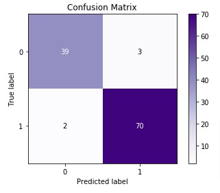
3. Classification Report (Precision, Recall, and F1-Score)
Classification report metrics provide precision, recall, f1-score, and support for each class.
- Precision — It represents how many predictions of a particular class are actually of that class.
- Precision = TP / (TP+FP).
- Recall — It represents how many predictions of a particular class are right.
- Recall = TP / (TP+FN).
- f1-score — It’s geometric average of precision & recall.
- F1-Score = 2 (Precision recall) / (Precision + recall)
- support — It represents number of occurrences of particular class in Y_true
Below, we have included a visualization that gives an exact idea about precision and recall.
Scikit-learn provides various functions to calculate precision, recall and f1-score metrics.
- precision_score() — Calculates overall precision.
- recall_score() — Calculates overall recall.
- f1-score() — Calculates overall f1-score.
- precision_recall_fscore_support() — Calculates precision, recall and f1-score per target class.
- classification_report() — Calculates precision, recall and f1-score per target class.
from sklearn.metrics import classification_report, precision_score, recall_score, f1_score, precision_recall_fscore_support

print('Precision                                   : %.3f'%precision_score(Y_test, Y_preds))
print('Recall                                      : %.3f'%recall_score(Y_test, Y_preds))
print('F1-Score                                    : %.3f'%f1_score(Y_test, Y_preds))
Precision                                   : 0.959
Recall                                      : 0.972
F1-Score                                    : 0.966
print('nPrecision Recall F1-Score Support Per Class : n',precision_recall_fscore_support(Y_test, Y_preds))
Precision Recall F1-Score Support Per Class :
 (array([0.95, 0.96]), array([0.93, 0.97]), array([0.94, 0.97]), array([42, 72]))
print('nClassification Report : ')
print(classification_report(Y_test, Y_preds))
Classification Report :
              precision    recall  f1-score   support

           0       0.95      0.93      0.94        42
           1       0.96      0.97      0.97        72

    accuracy                           0.96       114
   macro avg       0.96      0.95      0.95       114
weighted avg       0.96      0.96      0.96       114
4. ROC Curves & ROC AUC
ROC(Receiver Operating Characteristic) Curve helps better understand the performance of the model when handling an unbalanced dataset.
ROC Curve works with the output of prediction function or predicted probabilities by setting different threshold values to classify examples. It then calculates different false positives rates (FPR) and true positive rates (TPR) according to set threshold values. We can then plot a line chart with Y-axis as TPR and X-axis as FPR. The area under the line is generally referred to as ROC AUC (ROC Area Under Curve).
E.g., The output of binary classification model is probability in range 0-1. We can try different threshold values (0.2,0.35, 0.5, 0.65, 0.8, 0.95) to classify examples. Based on selected threshold value, the example with probability less than threshold is classified as negative class and greater than is classifier as positive class. This way we’ll get different positives and negatives for each threshold.
In the case of SVC, for example, a threshold set for output of decision function is 0 whereas ROC Curve tries various values for thresholds like [2,1,-1,-2] including negative threshold values as well.
In the case of LogisticRegression, the default threshold is 0.5 and ROC will try different threshold values.
For linear regression, the output is a probability between [0,1] hence threshold is set at 0.5 to differentiate positive/negative classes whereas in case of SVC internal kernel function returns a value, and threshold is set on that value for making a prediction.
Note: It’s restricted to binary classification tasks.
Scikit-learn provides various metrics to calculate ROC and ROC AUC metrics.
- roc_curve() — It takes actual labels and output of decision_function() or predict_proba() as input. It then returns TPR and FPR along with different threshold values that were tried. We can create line plot explained earlier using these TPR and FPR values.
- roc_auc_score() — It works like roc_curve() but returns area under the curve.
Below, we have explained how to calculate ROC & ROC AUC using sklearn. We can use either predict_proba() or decision_function() for calculation.
from sklearn.metrics import roc_curve, roc_auc_score

#fpr, tpr, thresholds = roc_curve(Y_test, log_reg.predict_proba(X_test)[:, 1])
fpr, tpr, thresholds = roc_curve(Y_test, log_reg.decision_function(X_test))

#auc = roc_auc_score(Y_test, log_reg.predict_proba(X_test)[:,1])
auc = roc_auc_score(Y_test, log_reg.decision_function(X_test))

acc = log_reg.score(X_test, Y_test)

print("False Positive Rates : {}".format(fpr))
print("True  Positive Rates : {}".format(tpr))
print("Threshols            : {}".format(thresholds))
print("Accuracy             : {:.3f}".format(acc))
print("AUC                  : {:.3f}".format(auc))
False Positive Rates : [0.   0.   0.   0.02 0.02 0.05 0.05 0.07 0.07 0.14 0.14 1.  ]
True  Positive Rates : [0.   0.01 0.62 0.62 0.93 0.93 0.97 0.97 0.99 0.99 1.   1.  ]
Threshols            : [  9.94   8.94   3.9    3.86   1.67   1.49   0.45   0.32  -0.43  -1.21
  -1.88 -41.37]
Accuracy             : 0.956
AUC                  : 0.988
Below, we have plotted ROC using matplotlib.
with plt.style.context(('ggplot','seaborn')):
    plt.figure(figsize=(8,6))
    plt.scatter(fpr, tpr, c='blue')
    plt.plot(fpr, tpr, label="Accuracy:%.2f AUC:%.2f" % (acc, auc), linewidth=2, c='red')
    plt.xlabel("False Positive Rate")
    plt.ylabel("True Positive Rate (recall)")
    plt.title('ROC Curve')
    plt.legend(loc='best');
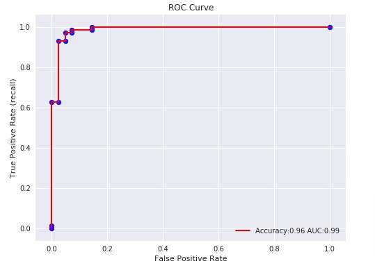
Below, we have plotted ROC using Python library scikit-plot.
skplt.metrics.plot_roc_curve(Y_test, log_reg.predict_proba(X_test),
                             title="ROC Curve", figsize=(12,6));
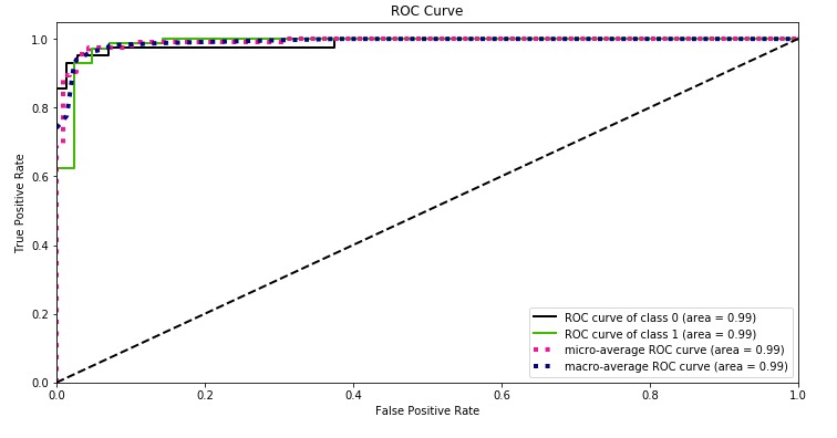
With a very small decision threshold, there will be few false positives, but also few false negatives, while with a very high threshold, both true positive rate and the false positive rate will be high.
So in general, the curve will be from the lower left to the upper right. A diagonal line reflects chance performance, while the goal is to be as much in the top left corner as possible. We want ROC Curve to cover almost 100% area for good performance. 50% area coverage refers to the chance model (random prediction).
5. Precision-Recall Curve
Precision and Recall help a lot in case of imbalanced datasets. It works exactly like ROC curve but uses precision and recall values.
Plotting different values of precision vs recall by setting different thresholds helps in evaluating the performance of the model better in case of imbalance classes. It does not take into consideration true negatives as it’s majority class and True positives represent minority class which has quite a few occurrences.
Note: It’s restricted to binary classification tasks.
Scikit-learn provides various metrics to calculate Precision-Recall Curve and Precision-Recall Curve AUC metrics.
- precision_recall_curve() — It takes actual labels and output of decision_function() or predict_proba() as input. It then returns precision and recall along with different threshold values that were tried. We can create line plot explained earlier using these precision and recall values.
- auc() — It works like precision_recall_curve() but returns area under the curve.
Below, we have explained how to calculate precision-recall curve & precision-recall AUC using sklearn. We can use either predict_proba() or decision_function() for calculation.
from sklearn.metrics import precision_recall_curve, auc,average_precision_score

#precision, recall, thresholds = precision_recall_curve(Y_test, log_reg.predict_proba(X_test)[:,1])
precision, recall, thresholds = precision_recall_curve(Y_test, log_reg.decision_function(X_test))

acc = log_reg.score(X_test, Y_test)

p_auc = auc(recall, precision)

print("Precision : {}".format(precision))
print("Recall    : {}".format(recall))
print("Threshols : {}".format(thresholds))
print("Accuracy  : {:.3f}".format(acc))
print("AUC       : {:.3f}".format(p_auc))
Precision : [0.92 0.92 0.93 0.95 0.96 0.96 0.97 0.97 0.97 0.97 0.99 0.99 0.98 0.98
 0.98 0.98 0.98 0.98 0.98 0.98 0.98 0.98 0.98 0.98 0.98 0.98 0.98 0.98
 0.98 0.98 0.98 0.98 0.98 1.   1.   1.   1.   1.   1.   1.   1.   1.
 1.   1.   1.   1.   1.   1.   1.   1.   1.   1.   1.   1.   1.   1.
 1.   1.   1.   1.   1.   1.   1.   1.   1.   1.   1.   1.   1.   1.
 1.   1.   1.   1.   1.   1.   1.   1.   1.  ]
Recall    : [1.   0.99 0.99 0.99 0.99 0.97 0.97 0.96 0.94 0.93 0.93 0.92 0.9  0.89
 0.88 0.86 0.85 0.83 0.82 0.81 0.79 0.78 0.76 0.75 0.74 0.72 0.71 0.69
 0.68 0.67 0.65 0.64 0.62 0.62 0.61 0.6  0.58 0.57 0.56 0.54 0.53 0.51
 0.5  0.49 0.47 0.46 0.44 0.43 0.42 0.4  0.39 0.38 0.36 0.35 0.33 0.32
 0.31 0.29 0.28 0.26 0.25 0.24 0.22 0.21 0.19 0.18 0.17 0.15 0.14 0.12
 0.11 0.1  0.08 0.07 0.06 0.04 0.03 0.01 0.  ]
Threshols : [-1.88 -1.21 -0.74 -0.43 -0.43  0.32  0.45  1.17  1.28  1.49  1.67  1.99
  2.08  2.27  2.31  2.32  2.61  2.67  2.69  2.88  2.91  2.92  3.03  3.13
  3.18  3.37  3.42  3.57  3.67  3.69  3.74  3.8   3.86  3.9   3.92  3.95
  4.08  4.39  4.79  4.82  4.85  4.91  4.93  4.94  5.02  5.14  5.2   5.2
  5.24  5.25  5.43  5.56  5.6   5.6   5.61  5.63  5.73  5.73  5.77  6.24
  6.24  6.32  6.36  6.42  6.58  6.64  6.71  6.79  6.87  6.99  7.7   7.82
  8.28  8.29  8.41  8.46  8.79  8.94]
Accuracy  : 0.956
AUC       : 0.992
Below, we have plotted Precision Recall Curve using matplotlib.
with plt.style.context(('ggplot', 'seaborn')):
    plt.figure(figsize=(8,6))
    plt.scatter(recall, precision, c='blue')
    plt.plot(recall, precision, label="Accuray:%.2f, AUC:%.2f" % (acc, p_auc), linewidth=2, c='red')
    plt.hlines(0.5,0.0,1.0, linestyle='dashed', colors=['orange'])
    plt.xlabel("Recall (Sensitivity)")
    plt.ylabel("Precision")
    plt.title('Precision Recall Curve')
    plt.legend(loc='best');
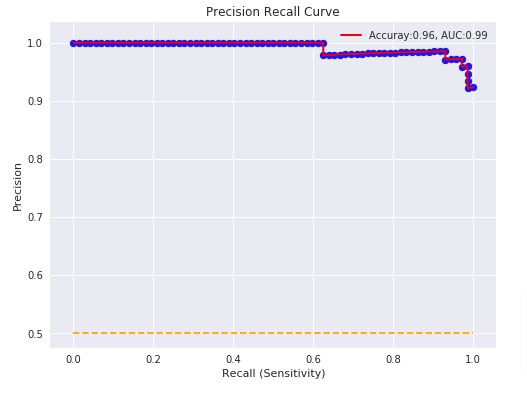
Below, we have plotted Precision Recall Curve using Python library scikit-plot.
skplt.metrics.plot_precision_recall_curve(Y_test, log_reg.predict_proba(X_test),
                             title="Precision Recall Curve", figsize=(12,6));
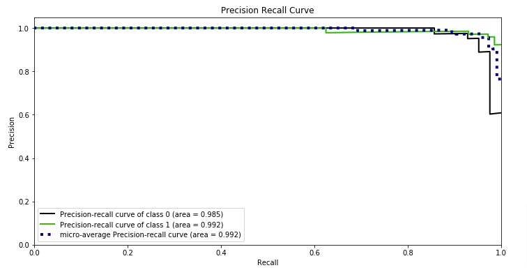
What to Use for Imbalanced Dataset (ROC AUC or Precision Recall AUC)?
Precision-recall curve totally crashes if our model is not performing well in case of an imbalanced dataset. ROC curves sometimes give optimistic results hence it’s better to consider precision-recall curves as well in case of imbalanced datasets. We recommend looking at classification reports as well for imbalanced datasets.
6. Log Loss (Logistic Loss or Cross-Entropy Loss)
Log loss refers to the negative log-likelihood of true labels predicted by the classifier. It’s a cost function whose output classifiers try to minimize while updating weights of the model.
log_loss = - y * log (y_probs) - (1-y) * log(1 - y_probs)
Scikit-learn provides a function named log_loss() through ‘metrics’ sub-module for calculating log loss. We need to provide actual target labels and predicted probabilities for calculating log loss to function.
from sklearn.metrics import log_loss

print('Test Log Loss   : %.3f'%log_loss(Y_test, log_reg.predict_proba(X_test)))
print('Train Log Loss  : %.3f'%log_loss(Y_train, log_reg.predict_proba(X_train)))
Test Log Loss   : 0.117
Train Log Loss  : 0.131
7. Zero One Classification Loss
It returns a number of misclassifications or a fraction of misclassifications. It accepts normalize parameter whose value if set True then returns a fraction of misclassifications else if set to False then it returns misclassifications.
Scikit-learn provides function named ‘zero_one_loss()’ function through ‘metrics’ sub-module. We need to provide actual and predicted target labels to calculate zero one classification loss.
from sklearn.metrics import zero_one_loss

print('Number of Misclassificied Examples   : ',zero_one_loss(Y_test, Y_preds, normalize=False))
print('Fraction of Misclassificied Examples : ',zero_one_loss(Y_test, Y_preds))
Number of Misclassificied Examples   :  5
Fraction of Misclassificied Examples :  0.04385964912280704
8. Balanced Accuracy Score
It returns an average recall of each class in classification problem. It’s useful to deal with imbalanced datasets.
It has parameter adjusted which when set True results are adjusted for a chance so that the random performing model would get a score of 0 and perfect performance will get 1.0.
We can calculate balanced accuracy using ‘balanced_accuracy_score()’ function of ‘sklearn.metrics’ module. We need to provide actual and predicted labels to function.
from sklearn.metrics import balanced_accuracy_score

print('Balanced Accuracy          : ',balanced_accuracy_score(Y_test, Y_preds))
print('Balanced Accuracy Adjusted : ',balanced_accuracy_score(Y_test, Y_preds, adjusted=True))
Balanced Accuracy          :  0.9503968253968254
Balanced Accuracy Adjusted :  0.9007936507936507
9. Brier Loss
It computes squared differences between the actual labels of class and predicted probability by model. It should be as low as possible for good performance. It’s for binary classification problems only. It by default takes 1 as a positive class hence if one needs to consider 0 as a positive class then one can use the pos_label parameter as below.
We can calculate brier loss using ‘brier_score_loss()’ from scikit-learn. We need to provide actual target labels and predicted probabilities of positive class to it.
from sklearn.metrics import brier_score_loss

print('Brier Loss                       : ',brier_score_loss(Y_test, log_reg.predict_proba(X_test)[:,1]))
print('Brier Loss (0 as Positive Class) : ', brier_score_loss(Y_test, log_reg.predict_proba(X_test)[:,1], pos_label=0))
Brier Loss                       :  0.03311574676769366
Brier Loss (0 as Positive Class) :  0.9039430558160102
10. F-Beta Score
F-Beta score refers to a weighted average of precision and recall based on the value of the beta parameter provided. If beta < 1 then it lends more weight to precision, while beta > 1 lends more weight to recall. It has the best value of 1.0 and the worst 0.0.
It has a parameter called average which is required for multiclass problems. It accepts values [None, ‘binary'(default), ‘micro’, ‘macro’, ‘samples’, ‘weighted’]. If None is specified then the score for each class is returned else average as per parameter is returned in a multi-class problem.
We can calculate F-beta score using fbeta_score() function of scikit-learn.
from sklearn.metrics import fbeta_score

print('Fbeta Favouring Precision : ', fbeta_score(Y_test, Y_preds, beta=0.5))
print('Fbeta Favouring Recall    : ' ,fbeta_score(Y_test, Y_preds, beta=2.0))
Fbeta Favouring Precision :  0.9615384615384616
Fbeta Favouring Recall    :  0.9695290858725762
11. Hamming Loss
It returns a fraction of labels misclassified. We can calculate hamming loss using hamming_loss() function of scikit-learn.
from sklearn.metrics import hamming_loss

print('Hamming Loss : ', hamming_loss(Y_test, Y_preds))
Hamming Loss : 0.043859649122807015
2. Regression Metrics 
In this section, we’ll introduce model evaluation metrics for regression tasks. We’ll first train a simple regression model and then evaluate its performance by calculating various regression metrics.
If you want to learn how to handle regression tasks using scikit-learn then please check below link. It covers topic in detail.
Supervised Learning: Regression using Scikit-Learn
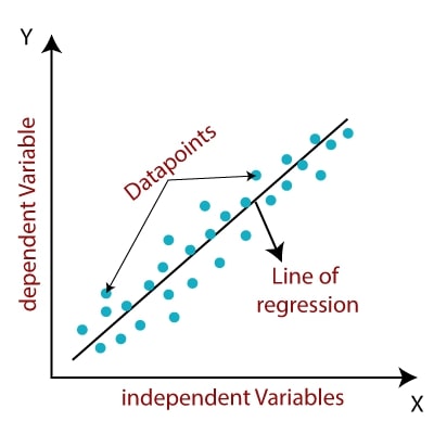
2.1 Load Data and Train Model
We’ll start with loading the Boston dataset available in scikit-learn for our purpose.
We’ll be splitting a dataset into train/test sets with 80% for a train set and 20% for the test set.
We’ll now initialize a simple LinearSVR model and train it on the train dataset. We’ll then check its performance by evaluating various regression metrics provided by scikit-learn.
from sklearn.linear_model import LinearRegression

boston = datasets.load_boston()

X, Y = boston.data, boston.target

print('Dataset Size : ', X.shape, Y.shape)

X_train, X_test, Y_train, Y_test = train_test_split(X, Y, train_size=0.90, random_state=123)

print('Train/Test Size : ', X_train.shape, X_test.shape, Y_train.shape, Y_test.shape)

lin_reg = LinearRegression()

lin_reg.fit(X_train, Y_train)
Dataset Size :  (506, 13) (506,)
Train/Test Size :  (455, 13) (51, 13) (455,) (51,)
Y_preds = lin_reg.predict(X_test)
2.2 Evaluate ML Metrics for Regression Tasks
1. R2 Score (Coefficient Of Determination)
The coefficient of R2 is defined as below.
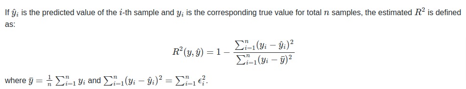
The R2 score generally has values in the range 0-1. The values near 1 are considered signs of a good model.
The best possible score is 1.0 and it can be negative as well if the model is performing badly. A model that outputs constant prediction for each input will have a score of 0.0.
The majority of the regression model’s score() method outputs this metric which is quite different from MSE(mean square error). Hence both should not be confused.
Scikit-learn provides function named ‘r2_score()’ through ‘metrics’ sub-module to calculate R2 score.
from sklearn.metrics import r2_score

print(Y_preds[:10])
print(Y_test[:10])

print('Test R^2     : %.3f'%r2_score(Y_test, Y_preds))
print('Test R^2     : %.3f'%lin_reg.score(X_test, Y_test))
print('Training R^2 : %.3f'%lin_reg.score(X_train, Y_train))
[14.74 27.68 38.87 18.01 30.24 36.72 25.13 10.16 15.59 31.95]
[15.  26.6 45.4 20.8 34.9 21.9 28.7  7.2 20.  32.2]
Test R^2     : 0.641
Test R^2     : 0.641
Training R^2 : 0.751
Below we are doing a grid search through various values of parameter C of LinearSVR and using r2 as an evaluation metric whose value will be optimized.
If you do not have a background on Grid search and want to learn about it then we would recommend you to check below link in your free time. It’ll help you with the concept.
- Scikit-Learn: Hyperparameters Tuning Using Grid Search
from sklearn.ensemble import GradientBoostingRegressor, RandomForestRegressor
from sklearn.model_selection import GridSearchCV

grid = GridSearchCV(GradientBoostingRegressor(),
                    param_grid = {'max_depth': [None, 3, 4, 6]},
                    scoring="r2", cv=5)
grid.fit(X, Y)

print('Best Parameters : ',grid.best_params_)
print('Best Score      : ',grid.best_score_)
print('Test R^2        : %.3f'%r2_score(Y_test, grid.best_estimator_.predict(X_test)))
print('Test R^2        : %.3f'%grid.best_estimator_.score(X_test, Y_test))
print('Training R^2    : %.3f'%grid.best_estimator_.score(X_train, Y_train))

Y_preds = grid.best_estimator_.predict(X_test)

print(Y_preds[:10])
print(Y_test[:10])
Best Parameters :  {'max_depth': 3}
Best Score      :  0.6818604620676322
Test R^2        : 0.985
Test R^2        : 0.985
Training R^2    : 0.974
[16.29 26.01 45.85 19.33 33.51 23.89 26.79  8.29 18.75 31.  ]
[15.  26.6 45.4 20.8 34.9 21.9 28.7  7.2 20.  32.2]
2. Mean Absolute Error (MAE)
Mean absolute error is a simple sum of the absolute difference between actual and predicted target value divided by a number of samples.
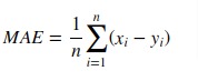
Scikit-learn provides function named ‘mean_absolute_error()’ through ‘metrics’ sub-module to calculate mean absolute error.
from sklearn.metrics import mean_absolute_error

print('Test MAE  : %.3f'%mean_absolute_error(Y_test, Y_preds))
print('Train MAE : %.3f'%mean_absolute_error(Y_train, lin_reg.predict(X_train)))
Test MAE  : 1.047
Train MAE : 3.103
Below we are doing a grid search through various values of parameter C of LinearSVR and using neg_mean_absolute_error as an evaluation metric whose value will be optimized.
grid = GridSearchCV(GradientBoostingRegressor(),
                    param_grid = {'max_depth': [None, 3, 4, 6]},
                    scoring="r2", cv=5)
grid.fit(X, Y)

print('Best Parameters : ',grid.best_params_)
print('Test MAE        : %.3f'%mean_absolute_error(Y_test, grid.best_estimator_.predict(X_test)))
print('Train MAE       : %.3f'%mean_absolute_error(Y_train, grid.best_estimator_.predict(X_train)))
Y_preds = grid.best_estimator_.predict(X_test)

print(Y_preds[:10])
print(Y_test[:10])
Best Parameters :  {'max_depth': 3}
Test MAE        : 1.047
Train MAE       : 1.122
[16.29 26.01 45.85 19.33 33.51 23.89 26.79  8.29 18.75 31.  ]
[15.  26.6 45.4 20.8 34.9 21.9 28.7  7.2 20.  32.2]
3. Mean Squared Error (MSE)
Mean Squared Error loss function simple sum of the squared difference between actual and predicted values divided by a number of samples.
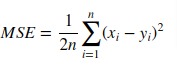
Scikit-learn provides function named ‘mean_squared_error()’ through ‘metrics’ sub-module to calculate mean squared error.
from sklearn.metrics import mean_squared_error, mean_squared_log_error

print('Test MSE  : %.3f'%mean_squared_error(Y_test, Y_preds))
print('Train MSE : %.3f'%mean_squared_error(Y_train, lin_reg.predict(X_train)))
Test MSE  : 1.693
Train MSE : 19.971
Below we are doing grid search through various values of parameter C of LinearSVR and using neg_mean_squared_error as an evaluation metric whose value will be optimized.
grid = GridSearchCV(GradientBoostingRegressor(),
                    param_grid = {'max_depth': [None, 3, 4, 6]},
                    scoring="r2", cv=5)
grid.fit(X, Y)

print('Best Parameters : ',grid.best_params_)
print('Test MSE        : %.3f'%mean_squared_error(Y_test, grid.best_estimator_.predict(X_test)))
print('Train MSE       : %.3f'%mean_squared_error(Y_train, grid.best_estimator_.predict(X_train)))
Y_preds = grid.best_estimator_.predict(X_test)

print(Y_preds[:10])
print(Y_test[:10])
Best Parameters :  {'max_depth': 3}
Test MSE        : 1.693
Train MSE       : 2.050
[16.29 26.01 45.85 19.33 33.51 23.89 26.79  8.29 18.75 31.  ]
[15.  26.6 45.4 20.8 34.9 21.9 28.7  7.2 20.  32.2]
4. Mean Squared Log Error
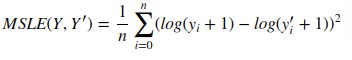
It can not be used when target contains negative values/predictions.
Scikit-learn provides function named ‘mean_squared_log_error()’ through ‘metrics’ sub-module to calculate mean squared log error.
from sklearn.metrics import mean_squared_log_error

print("Mean Squared Log Error : {:.3f}".format(mean_squared_log_error(Y_test, Y_preds)))
Mean Squared Log Error : 0.003
5. Median Absolute Error

Scikit-learn provides function named ‘median_absolute_error()’ through ‘metrics’ sub-module to calculate median absolute error.
from sklearn.metrics import median_absolute_error

print('Median Absolute Error : {}'.format(median_absolute_error(Y_test, Y_preds)))
print('Median Absolute Error : {}'.format(np.median(np.abs(Y_test - Y_preds))))
Median Absolute Error : 0.8607557405323369
Median Absolute Error : 0.8607557405323369
6. Explained Variance Score
It returns the explained variance regression score. The best value is 1.0 and fewer values refer to a bad model.
Scikit-learn provides function named ‘explained_variance_score()’ through ‘metrics’ sub-module to calculate explained variance score.
from sklearn.metrics import explained_variance_score

print('Explained Variance Score : {:.3f}'.format(explained_variance_score(Y_test, Y_preds)))
Explained Variance Score : 0.985
7. Residual Error
It returns the max of the difference between actual values and the predicted value of all samples.
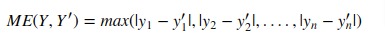
Scikit-learn provides function named ‘max_error()’ through ‘metrics’ sub-module to calculate residual error.
from sklearn.metrics import max_error

print('Maximum Residual Error : {:.3f}'.format(max_error(Y_test, Y_preds)))
print('Maximum Residual Error : {:.3f}'.format(max_error([1,2,3,4], [1,2,3.5,7]))) ## here 4th sample has highest difference
Maximum Residual Error : 3.759
Maximum Residual Error : 3.000
3. Clustering Metrics 
We’ll now introduce evaluation metrics for unsupervised learning — clustering tasks. We’ll train a simple ML model for solving clustering task and then evaluate its performance by calculating various metrics.
If you want to learn about clustering then we would recommend you to go through below link as it covers topic in detail.
Unsupervised Learning: Clustering using Scikit-Learn

3.1 Load Data and Train Model
from sklearn.cluster import KMeans, MeanShift
from sklearn.datasets import load_iris
from sklearn.metrics import accuracy_score, adjusted_rand_score, confusion_matrix

iris = load_iris()
X, Y = iris.data, iris.target

X_train, X_test, Y_train, Y_test = train_test_split(X, Y, train_size=0.80, test_size=0.20, stratify=Y, random_state=12)
print('Train/Test Sizes  : ', X_train.shape, X_test.shape, Y_train.shape, Y_test.shape)

kmeans = KMeans(n_clusters=3)

kmeans.fit(X_train, Y_train)
Train/Test Sizes : (120, 4) (30, 4) (120,) (30,)
3.2 Evaluate ML Metrics for Clustering Tasks
1. Adjusted Rand Score
Clustering algorithms return cluster labels for each cluster specified but they might not return in the same sequence as original labels. It might happen that in the original dataset some class has samples labeled as 1 and in predictions by cluster, an algorithm can label it as other than 1.
We’ll use the IRIS dataset and KMeans for explanation purposes. We’ll even plot results to show the difference. We’ll show accuracy will improve once we use ‘adjusted_rand_score()’ as an evaluation function.
Y_preds = kmeans.predict(X_test) print('Confusion Matrix : ') print(confusion_matrix(Y_test, Y_preds)) print('Accuracy of Model : %.3f'%accuracy_score(Y_test, Y_preds)) print('Adjusted Accuracy : %.3f'%adjusted_rand_score(Y_test, Y_preds))
Confusion Matrix : [[ 0 10 0] [ 0 0 10] [ 8 0 2]] Accuracy of Model : 0.067 Adjusted Accuracy : 0.808
with plt.style.context(('ggplot', 'seaborn')): plt.figure(figsize=(10,4)) plt.subplot(121) plt.scatter(X_test[: , 1], X_test[:, 2], c=Y_test, cmap = plt.cm.viridis) plt.xlabel(iris.feature_names[1]) plt.ylabel(iris.feature_names[2]) plt.title('Y Original') plt.subplot(122) plt.scatter(X_test[: , 1], X_test[:, 2], c=Y_preds, cmap = plt.cm.viridis) plt.xlabel(iris.feature_names[1]) plt.ylabel(iris.feature_names[2]) plt.title('Y Predicted');

4. How to Create Custom Metric/Scoring Function? 
Users can also define their own scoring function if their scoring function is not available in built-in scoring functions of sklearn. In GridSearchCV and cross_val_score, one can provide object which has call method or function to scoring parameter. Object or function both need to accept estimator object, test features(X) and target(Y) as input, and return float.
Below we are defining RMSE (Root Mean Squared Error) as a class and as a function as well. We’ll then use it in cross_val_score() to check performance also compares it’s value with negative of neg_mean_squared_error.
boston = datasets.load_boston() X, Y = boston.data, boston.target X_train, X_test, Y_train, Y_test = train_test_split(X, Y, train_size=0.80, test_size=0.20, random_state=1, )
from sklearn.linear_model import LinearRegression
from sklearn.model_selection import cross_val_score class RootMeanSquareError(object): def __call__(self, model, X, Y): Y_preds = model.predict(X) return np.sqrt(((Y - Y_preds)**2).mean()) def rootMeanSquareError(model, X, Y): Y_preds = model.predict(X) return np.sqrt(((Y - Y_preds)**2).mean()) lin_reg = LinearRegression() lin_reg.fit(X_train, Y_train) rmse_obj = RootMeanSquareError() print("Train RMSE : {}".format(rmse_obj(lin_reg, X_train, Y_train))) print("Train RMSE : {}".format(rootMeanSquareError(lin_reg, X_train, Y_train))) print("nTest RMSE : {}".format(rmse_obj(lin_reg, X_test, Y_test))) print("Test RMSE : {}".format(rootMeanSquareError(lin_reg, X_test, Y_test)))
Train RMSE : 4.675766751547772 Train RMSE : 4.675766751547772 Test RMSE : 4.835373458200514 Test RMSE : 4.835373458200514
Custom Metrics with Cross Validation
Below, we have explained how to use custom metrics with scikit-learn function cross_val_score().
If you are someone who does not have background on cross validation then we would recommend you to check below link.
- Scikit-Learn: Cross Validation
rmse1 = cross_val_score(lin_reg, X, Y, scoring=RootMeanSquareError()) rmse2 = cross_val_score(lin_reg, X, Y, scoring=rootMeanSquareError) rmse3 = np.sqrt(-1*cross_val_score(lin_reg, X, Y, scoring='neg_mean_squared_error')) print('Cross Val Score Using Object : {}'.format(rmse1)) print('Cross Val Score Using Function : {}'.format(rmse2)) print('Cross Val Score Using Square Root of Neg Mean Squared Error : {}'.format(rmse3))
Cross Val Score Using Object : [3.53 5.1 5.75 8.99 5.77] Cross Val Score Using Function : [3.53 5.1 5.75 8.99 5.77] Cross Val Score Using Square Root of Neg Mean Squared Error : [3.53 5.1 5.75 8.99 5.77]
Custom Metrics with Grid Search
Below, we have explained how to use custom metrics with grid search.
If you are someone who does not have background on grid search then we would recommend you to check below link.
- Scikit-Learn: Hyperparameters Tuning Using Grid Search
from sklearn.model_selection import GridSearchCV from sklearn.ensemble import GradientBoostingRegressor from sklearn.metrics import mean_squared_error grid = GridSearchCV(GradientBoostingRegressor(), param_grid = {'max_depth': [3, 4, 6]}, scoring=RootMeanSquareError(), cv=5) grid.fit(X_train, Y_train) print('Best Parameters : ',grid.best_params_) print("Best MSE : {:5f}".format(grid.best_score_)) print('Test MSE : {:.5f}'.format(mean_squared_error(Y_test, grid.best_estimator_.predict(X_test)))) print('Train MSE : {:.5f}'.format(mean_squared_error(Y_train, grid.best_estimator_.predict(X_train)))) Y_preds = grid.best_estimator_.predict(X_test) print(Y_preds[:10]) print(Y_test[:10])
Best Parameters : {'max_depth': 3}
Best MSE : 3.344041
Test MSE : 7.78709
Train MSE : 1.78408
[31.1 26.8 18.79 20.58 20.1 20.35 29.17 18.89 20.99 24.44]
[28.2 23.9 16.6 22. 20.8 23. 27.9 14.5 21.5 22.6]
5. List of All Metrics available from Scikit-Learn 
Below are list of scikit-learn builtin functions.
print('List of Inbuilt Scorers : n') for metric in sklearn.metrics.SCORERS: print(metric)
List of Inbuilt Scorers : explained_variance r2 max_error neg_median_absolute_error neg_mean_absolute_error neg_mean_absolute_percentage_error neg_mean_squared_error neg_mean_squared_log_error neg_root_mean_squared_error neg_mean_poisson_deviance neg_mean_gamma_deviance accuracy top_k_accuracy roc_auc roc_auc_ovr roc_auc_ovo roc_auc_ovr_weighted roc_auc_ovo_weighted balanced_accuracy average_precision neg_log_loss neg_brier_score adjusted_rand_score rand_score homogeneity_score completeness_score v_measure_score mutual_info_score adjusted_mutual_info_score normalized_mutual_info_score fowlkes_mallows_score precision precision_macro precision_micro precision_samples precision_weighted recall recall_macro recall_micro recall_samples recall_weighted f1 f1_macro f1_micro f1_samples f1_weighted jaccard jaccard_macro jaccard_micro jaccard_samples jaccard_weighted
This ends our small tutorial explaining how to use various ML metrics available from ‘metrics’ sub-module of ‘sklearn’ to evaluate performance of ML Models trained on classification, regression and clustering tasks.
> Are ML Metrics Enough to Evaluate Model Performance?
Though ML Metrics are a good starting point for evaluating performance of ML Models, sometimes they are not enough. There can be situations when ML metrics are giving good numbers indicating a good model but in reality, our model has not generalized.
> Should you Interpret Predictions of Model?
That’s where various algorithms to interpret predictions of ML models come in handy. They let us see which features are contributing to predictions. What is intensity of various features towards predictions? This can helps us make even more informed decisions.
We would recommend that you read our tutorials for interpreting predictions of ML Models listed below in references section as it’ll help you evaluate model performance even better.
References
Libraries to Visualize ML Metrics
- Scikit-Plot: Visualize ML Metrics
- yellowbrick: Visualize Sklearn Classification and Regression Metrics
- yellowbrick: Text Data Visualizations
Python Libraries to Interpret Predictions of ML Models
- How to Use LIME to Interpret Predictions of ML Models?
- SHAP Values: Explain Predictions of ML Models using Game-Theoretic Approach
- How to Use ‘Eli5’ to Understand ML Models and their Predictions?
- captum: Interpret Predictions of PyTorch Networks
- Treeinterpreter: Interpreting Tree-Based Model’s Prediction of Individual Sample
- interpret-ml: Explain ML Models and their Predictions
- interpret-text: Explain NLP Models
- dice-ml: Diverse Counterfactual Explanations for ML Models
Classification
Binary cross entropy
Binary cross entropy is a loss function used for binary classification tasks (tasks with only two outcomes/classes). It works by calculating the following average:
The above equation can be split into two parts to make it easier to understand:
The above graph shows that the further away the prediction is from the actual y value the bigger the loss gets.
That means that if the correct answer is 0, then the cost function will be 0 if the prediction is also 0. If the prediction approaches 1, then the cost function will approach infinity.
If the correct answer is 1, then the cost function will be 0 if the prediction is 1. If the prediction approaches 0, then the cost function will approach infinity.
Resources:
- Understanding Categorical Cross-Entropy Loss, Binary Cross-Entropy Loss, Softmax Loss, Logistic Loss, Focal Loss and all those confusing names
- Cross entropy
- Understanding binary cross-entropy / log loss: a visual explanation
Code:
- Binary Cross Entropy Numpy Implementation
Categorical Crossentropy
Categorical crossentropy is a loss function used for multi-class classification tasks. The outputed loss is the negative average of the sum of the true values multiplied by the log of the predicted values .
Resources:
- Understanding Categorical Cross-Entropy Loss, Binary Cross-Entropy Loss, Softmax Loss, Logistic Loss, Focal Loss and all those confusing names
- Categorical crossentropy
Code:
- Categorical Cross Entropy Numpy Implementation
Accuracy Score
The fraction of predictions the model classified correctly.
or
For binary classification, accuracy can also be calculated in terms of positives and negatives as follows:
Where , , , and .
Resources:
- ‘Classification: Accuracy’ Google Machine Learning Crash Course
- Accuracy Score Scikit Learn
- Precision and recall
Code:
- Accuracy Score Numpy Implementation
Confusion matrix
A confusion matrix is a table that summarises the predictions of a classifier or classification model. By definition, entry in a confusion matrix is the number of observations actually in group , but predicted to be in group .
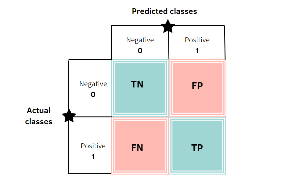
Resources:
- Confusion matrix Scikit-Learn
- What is a Confusion Matrix in Machine Learning
- Simple guide to confusion matrix terminology
Precision
Precision is a metric for classification models that identifies the frequency with which a model was correct when predicting the positive class. Precision is defined as the number of true positives over the number of true positives plus the number of false positives.
Resources:
- Precision, recall and F-measures
- Precision-Recall
- Precision Wikipedia
- Classification: Precision and Recall
- Accuracy, Precision, Recall or F1?
Code:
- Precision Numpy Implementation
Recall
Recall is a metric for classification models that identifies how many positive labels the model identified out of all the possible positive labels.
Resources:
- Precision, recall and F-measures
- Precision-Recall
- Precision Wikipedia
- Classification: Precision and Recall
- Accuracy, Precision, Recall or F1?
Code:
- Recall Numpy Implementation
F1-Score
The F1-Score is the harmonic mean of precision and recall. A perfect model will have an F1-Score of 1.
It’s also possible to weight precision or recall differently using the -Score. Here a real factor is used to weight the recall times as much as the precision.
Resources:
- Precision, recall and F-measures
- What is the F-score?
- Accuracy, Precision, Recall or F1?
- F-score Wikipedia
Code:
- F1-Score Numpy Implementation
- -Score Numpy Implementation
Receiver operating characteristic (ROC)
The ROC curve (receiver operating characteristic curve) is a graph that illustrates the performance of a classification model as its discrimination threshold is varied. The ROC curve is created by plotting the true positive rate (TPR) against the false positive rate (FPR) at various threshold settings.
True Positive Rate (TPR):
False Positive Rate (FPR):
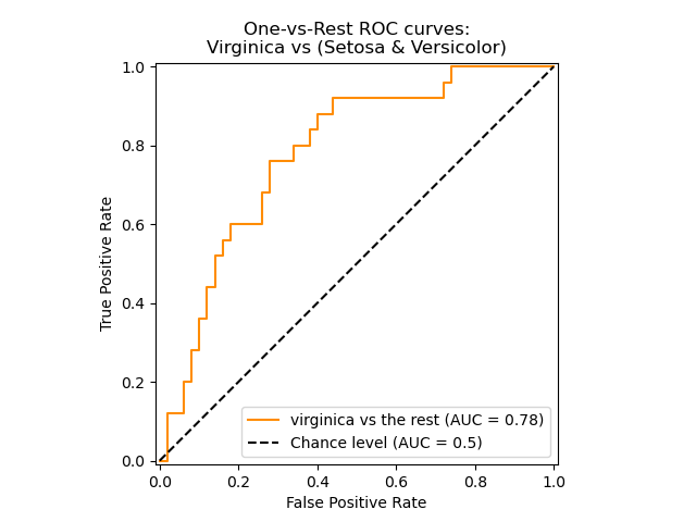
Resources:
- Receiver operating characteristic Wikipedia
- Receiver operating characteristic (ROC)
- Classification: ROC Curve and AUC
- Understanding AUC — ROC Curve
Area under the ROC curve (AUC)
AUC stands for «Area under the ROC Curve». AUC provides an aggregate measure of performance across all possible classification thresholds. One way of interpreting AUC is as the probability that the model ranks a random positive example more highly than a random negative example. — Google Developers Machine Learning Crash Course

Resources:
- Area under the curve Wikipedia
- Receiver operating characteristic (ROC)
- Classification: ROC Curve and AUC
- Understanding AUC — ROC Curve
Hinge Loss
Hinge loss is a loss function usef for «maximum-margin» classification, most notably for Support Vector Machines (SVMs).
Resources:
- Hinge Loss Scikit-Learn
- Hinge loss Wikipedia
- What is the definition of the hinge loss function?
Code:
- Hinge Loss Numpy Implementation
KL Divergence
The Kullback-Leibler divergence, , often shortenend to just KL divergence, is a measure of how one probability distribution is different from a second, reference porbability distribution.
Resources:
- Kullback–Leibler divergence Wikipedia
- Kullback-Leibler Divergence Explained
Code:
- KL Divergence Numpy Implementation
Brier Score
The Brier Score is a strictly proper score function or strictly proper scoring rule that measures the accuracy of probabilistic predictions. For unidimensional predictions, it is strictly equivalent to the mean squared error as applied to predicted probabilities. — Wikipedia
Resources:
- Brier Score Wikipedia
- Brier Score Loss Scikit-Learn
- Brier Score – How to measure accuracy of probablistic predictions
Code:
- Brier Score Numpy Implementation
Regression
Mean Squared Error
The mean squared error (MSE) or mean squared deviation (MSD) measure the average of the squares of the errors — that is, the average squared differences between the estimated and actual values.
Resources:
- Mean squared error Wikipedia
- Mean squared error Scikit-Learn
- Machine learning: an introduction to mean squared error and regression lines
Code:
- Mean Squared Error Numpy Implementation
Mean Squared Logarithmic Error
Mean Squared Logarithmic Error (MSLE) is an extension of Mean Squared Error (MSE) often used when the target has an exponential growth.
Note: This metrics penalizes under-predictions greater than over-predictions.
Code:
- Mean Squared Logarithmic Error Numpy Implementation
Resources:
- Mean squared logarithmic error (MSLE)
- Mean squared logaritmic error Scikit-Learn
- Understanding the metric: RMSLE
Mean Absolute Error
The mean absolute error (MAE) measure the average of the absolute values of the errors — that is, the average absolute differences between the estimated and actual values.
Code:
- Mean Absolute Error Numpy Implementation
Resources:
- Mean absolute error Wikipedia
- Mean absolute error Scikit-Learn
Mean Absolute Percentage Error
Mean absolute percentage error is an extension of the mean absolute error (MAE) that divides the difference between the predicted value and the actual value by the actual value. The main idea of MAPD is to be sensitive to relative errors. It’s for example not changed by a global scaling of the target variable.
Code:
- Mean Absolute Percentage Error Numpy Implementation
Resources:
- Mean absolute percentage error Wikipedia
- Mean absolute percentage error Scikit-Learn
Median Absolute Error
The median absolute error also often called median absolute deviation (MAD) is metric that is particularly robust to outliers. The loss is calculated by taking the median of all absolute differences between the target and the prediction.
Code:
- Median Absolute Error Numpy Implementation
Resources:
- Median absolute error Wikipedia
- Median absolute error Scikit-Learn
Cosine Similarity
Cosine similarity is a measure of similarity between two vectors. The cosine similarity is the cosine of the angle between two vectors.
Code:
- Cosine Similarity Numpy Implementation
Resources:
- Cosine Similarity Wikipedia
- Cosine Similarity – Understanding the math and how it works (with python codes)
R2 Score
The coefficient of determination, denoted as is the proportion of the variation in the dependent variable that has been explained by the independent variables in the model.
where
Code:
- R2 Score Numpy Implementation
Resources:
- Coefficient of determination Wikipedia
- R² score, the coefficient of determination Scikit-Learn
Tweedie deviance
The Tweedie distributions are a family of probability distributions, which include he purely continuous normal, gamma and Inverse Gaussian distributions and more.
The unit deviance of a reproductive Tweedie distribution is given by:
Code:
- Tweedie deviance Numpy Implementation
Resources:
- Tweedie distribution Wikipedia
- Mean Poisson, Gamma, and Tweedie deviances
D^2 score
The -Score computes the percentage of deviance explained. It is a generalization of , where the squared error is replaced by the Tweedie deviance. — Scikit Learn
, also known as McFadden’s likelihood ratio index, is calculated as
Code:
- D^2 Score Numpy Implementation
Resources:
- D² score, the coefficient of determination
Huber Loss
Huber loss is a loss function that is often used in robust regression. The function is quadratich for small values of and linear for large values.
where and is the point where the loss changes from a quadratic to linear.
Code:
- Huber Numpy Implementation
Resources:
- Huber loss Wikipedia
- Huber loss Tensorflow
Log Cosh Loss
Logarithm of the hyperbolic cosine of the prediction error.
Code:
- Log Cosh Loss Numpy Implementation
Resources:
- Log Cosh loss Tensorflow
From Wikipedia, the free encyclopedia
In statistics, mean absolute error (MAE) is a measure of errors between paired observations expressing the same phenomenon. Examples of Y versus X include comparisons of predicted versus observed, subsequent time versus initial time, and one technique of measurement versus an alternative technique of measurement. MAE is calculated as the sum of absolute errors divided by the sample size:[1]

It is thus an arithmetic average of the absolute errors  , where
  is the prediction and
  the true value. Note that alternative formulations may include relative frequencies as weight factors. The mean absolute error uses the same scale as the data being measured. This is known as a scale-dependent accuracy measure and therefore cannot be used to make comparisons between series using different scales.[2] The mean absolute error is a common measure of forecast error in time series analysis,[3] sometimes used in confusion with the more standard definition of mean absolute deviation. The same confusion exists more generally.
Quantity disagreement and allocation disagreement[edit]
2 data points for which Quantity Disagreement is 0 and Allocation Disagreement is 2 for both MAE and RMSE
It is possible to express MAE as the sum of two components: Quantity Disagreement and Allocation Disagreement. Quantity Disagreement is the absolute value of the Mean Error given by:[4]

Allocation Disagreement is MAE minus Quantity Disagreement.
It is also possible to identify the types of difference by looking at an  plot. Quantity difference exists when the average of the X values does not equal the average of the Y values. Allocation difference exists if and only if points reside on both sides of the identity line.[4][5]
[edit]
The mean absolute error is one of a number of ways of comparing forecasts with their eventual outcomes. Well-established alternatives are the mean absolute scaled error (MASE) and the mean squared error. These all summarize performance in ways that disregard the direction of over- or under- prediction; a measure that does place emphasis on this is the mean signed difference.
Where a prediction model is to be fitted using a selected performance measure, in the sense that the least squares approach is related to the mean squared error, the equivalent for mean absolute error is least absolute deviations.
MAE is not identical to root-mean square error (RMSE), although some researchers report and interpret it that way. MAE is conceptually simpler and also easier to interpret than RMSE: it is simply the average absolute vertical or horizontal distance between each point in a scatter plot and the Y=X line. In other words, MAE is the average absolute difference between X and Y. Furthermore, each error contributes to MAE in proportion to the absolute value of the error. This is in contrast to RMSE which involves squaring the differences, so that a few large differences will increase the RMSE to a greater degree than the MAE.[4] See the example above for an illustration of these differences.
Optimality property[edit]
The mean absolute error of a real variable c with respect to the random variable X is

Provided that the probability distribution of X is such that the above expectation exists, then m is a median of X if and only if m is a minimizer of the mean absolute error with respect to X.[6] In particular, m is a sample median if and only if m minimizes the arithmetic mean of the absolute deviations.[7]
More generally, a median is defined as a minimum of

as discussed at Multivariate median (and specifically at Spatial median).
This optimization-based definition of the median is useful in statistical data-analysis, for example, in k-medians clustering.
Proof of optimality[edit]
Statement: The classifier minimising  is
is  .
.
Proof:
The Loss functions for classification is
![{displaystyle {begin{aligned}L&=mathbb {E} [|y-a||X=x]\&=int _{-infty }^{infty }|y-a|f_{Y|X}(y),dy\&=int _{-infty }^{a}(a-y)f_{Y|X}(y),dy+int _{a}^{infty }(y-a)f_{Y|X}(y),dy\end{aligned}}}](https://wikimedia.org/api/rest_v1/media/math/render/svg/7e953e54457072620a7c2764db0801f69c4e883d)
Differentiating with respect to a gives

This means

Hence

See also[edit]
- Least absolute deviations
- Mean absolute percentage error
- Mean percentage error
- Symmetric mean absolute percentage error
References[edit]
- ^ Willmott, Cort J.; Matsuura, Kenji (December 19, 2005). «Advantages of the mean absolute error (MAE) over the root mean square error (RMSE) in assessing average model performance». Climate Research. 30: 79–82. doi:10.3354/cr030079.
- ^ «2.5 Evaluating forecast accuracy | OTexts». www.otexts.org. Retrieved 2016-05-18.
- ^ Hyndman, R. and Koehler A. (2005). «Another look at measures of forecast accuracy» [1]
- ^ a b c Pontius Jr., Robert Gilmore; Thontteh, Olufunmilayo; Chen, Hao (2008). «Components of information for multiple resolution comparison between maps that share a real variable». Environmental and Ecological Statistics. 15 (2): 111–142. doi:10.1007/s10651-007-0043-y. S2CID 21427573.
- ^ Willmott, C. J.; Matsuura, K. (January 2006). «On the use of dimensioned measures of error to evaluate the performance of spatial interpolators». International Journal of Geographical Information Science. 20: 89–102. doi:10.1080/13658810500286976. S2CID 15407960.
- ^ Stroock, Daniel (2011). Probability Theory. Cambridge University Press. pp. 43. ISBN 978-0-521-13250-3.
- ^ Nicolas, André (2012-02-25). «The Median Minimizes the Sum of Absolute Deviations (The $ {L}_{1} $ Norm)». StackExchange.
Once we build our regression model, how can we measure the goodness of fit?
We have various regression evaluation metrics to measure how well our model fits the data.
In this article, we will see some of the most commonly used metrics to asses the regression model.
MEAN SQUARED ERROR:
The first metric we are going to see is the mean squared error.
It calculates the average of the square of the errors between the actual and the predicted values.
Lower the value, better the regression model.

Here yi denotes the true score for the ith data point, and ŷi indicates the predicted value and n is the number of data points.
|
import numpy as np def mse(actual, predicted): return np.mean(np.square(actual—predicted)) |
However, the problem with MSE is since the values are squared, the unit of measurement is changed.
To overcome this problem, we use the root mean squared error.
ROOT MEAN SQUARED ERROR:
RMSE is the most popular metric to measure the error of a regression model.
This metric is calculated as the square root of the average squared distance between the actual and the predicted values.
Taking the square root of the mean squared error will give you RMSE.
Since we are, taking the square root it reverts the unit of measurement to its original scale.

It can be used to compare models only whose errors are measured in the same units.
|
def rmse(actual, predicted): return np.sqrt(np.mean(np.square(actual—predicted))) |
MEAN ABSOLUTE ERROR:
It is calculated as the mean of the absolute difference between the actual and the predicted values.

Where ŷi is the predicted value of the ith sample, and yi is the corresponding actual value, and N is the number of samples.
|
def mae(actual, predicted): return np.mean(np.abs(actual—predicted)) |
Both RMSE and MAE are scale dependent and can be used to compare models only if they are measured in the same units.
To compare models with different units, we can use metrics like MAPE or RAE.
MEAN ABSOLUTE PERCENTAGE ERROR(MAPE):
MAPE measures the error in percentage terms.
MAPE is calculated as the absolute difference between the actual and predicted values divide over every observation.

It is multiplied by 100 to make it a percentage error.
Where n is the size of the sample, ŷt is the value predicted by the model, and yt is the actual value.
|
def mape(actual, predicted): return np.mean(np.abs((actual — predicted) / actual)) * 100 |
However, the problem here is, it produces infinite or undefined values for zero or close-to-zero actual values.
RELATIVE ABSOLUTE ERROR:
RAE is defined as the ratio between the sum of absolute errors and the sum of absolute deviations.

pi is the predicted value, and ai is the actual value, and a_bar is the mean of actual values.
|
def rae(actual, predicted): numerator = np.sum(np.abs(predicted — actual)) denominator = np.sum(np.abs(np.mean(actual) — actual)) return numerator / denominator |
R-SQUARE:
R-square, also known as the coefficient of determination, is one of the commonly used regression evaluation metrics.
It measures the proportion of variance of the dependent variable explained by the independent variable.
If the R-squared value is 0.90, then we can say that the independent variables have explained 90% of the variance in the dependent variable.
It ranges from 0 to 1, where 0 indicates that the fit is poor.
It is determined as the ratio of the sum of squares and the total sum of squares,

where SSE is the sum of squared errors and computed as,

and SST(total sum of squares) is given as,

|
def r_squared(actual, predicted): sse = np.sum(np.square(actual—predicted)) sst = np.sum(np.square(actual—np.mean(actual))) return 1 — (sse/sst) |
However, the problem with r-square is that the value spuriously increases as more number of independent variables are added.
Even if the variables are irrelevant, the value of r-square will still increase.
Assume we are comparing two models A and B with the same dependent variable and A having more independent variables than model B.
Then there is a chance that the r-square value of model A is greater than or equal to model B just because model A has more independent variables.
So r-squared cannot be used for having meaningful comparison between models.
ADJUSTED R-SQUARE:
To counter the problem which is faced by r-square, Adjusted r-square penalizes adding more independent variables which don’t increase the explanatory power of the regression model.
The value of adjusted r-square is always less than or equal to the value of r-square.
It ranges from 0 to 1, the closer the value is to 1, the better it is.

n = the sample size
k = the number of independent variables
|
def adj_r_squared(X, actual, predicted): #X is your training dataset r_squ = r_squared(actual, predicted) numerator = 1 — (1 — r_squ) * len(actual)—1 denominator = len(actual) — X.shape[1]—1 #X.shape[1] will give number of independent variables return numerator/denominator |
MEDIAN ABSOLUTE ERROR:
Calculated as the median of all absolute differences between the actual and predicted values.
![]()
where yi is the actual value, and ŷ is the predicted value.
MAE is robust to outliers.
|
def median_abs_error(actual, predicted): return np.sum(np.median(np.abs(actual — predicted))) |
SUMMARY:
Performance metrics are vital for any machine learning model.
In this article, we discussed several important regression evaluation metrics.
We first discussed Mean Squared Error(MSE), which measures the average squared error of our predictions.
The problem with MSE is that since the values are squared the unit of measurement is changed.
To fill this deficiency, we looked at another metric called RMSE, which reverts the value to its original unit of measurement by taking a square root.
Then we discussed MAPE and RAE, which can be used to compare two models of different scales.
We then discussed r-squared and learned why it could not be used to have a sensible comparison between two models.
To counter the problem faced by r-squared, we discussed the adjusted r-squared.
Finally, we discussed Median Absolute Error, which is resilient to outliers.