Finding the median in sets of data with an odd and even number of values
In statistics and probability theory, the median is the value separating the higher half from the lower half of a data sample, a population, or a probability distribution. For a data set, it may be thought of as «the middle» value. The basic feature of the median in describing data compared to the mean (often simply described as the «average») is that it is not skewed by a small proportion of extremely large or small values, and therefore provides a better representation of the center. Median income, for example, may be a better way to describe center of the income distribution because increases in the largest incomes alone have no effect on median. For this reason, the median is of central importance in robust statistics.
Finite data set of numbers[edit]
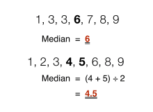
The median of a finite list of numbers is the «middle» number, when those numbers are listed in order from smallest to greatest.
If the data set has an odd number of observations, the middle one is selected. For example, the following list of seven numbers,
- 1, 3, 3, 6, 7, 8, 9
has the median of 6, which is the fourth value.
If the data set has an even number of observations, there is no distinct middle value and the median is usually defined to be the arithmetic mean of the two middle values.[1][2] For example, this data set of 8 numbers
- 1, 2, 3, 4, 5, 6, 8, 9
has a median value of 4.5, that is  . (In more technical terms, this interprets the median as the fully trimmed mid-range).
In general, with this convention, the median can be defined as follows: For a data set  of
of  elements, ordered from smallest to greatest,
- if
 is odd,
 - if is even,


| Type | Description | Example | Result |
|---|---|---|---|
| Midrange | Midway point between the minimum and the maximum of a data set | 1, 2, 2, 3, 4, 7, 9 | 5 |
| Arithmetic mean | Sum of values of a data set divided by number of values: 
|
(1 + 2 + 2 + 3 + 4 + 7 + 9) / 7 | 4 |
| Median | Middle value separating the greater and lesser halves of a data set | 1, 2, 2, 3, 4, 7, 9 | 3 |
| Mode | Most frequent value in a data set | 1, 2, 2, 3, 4, 7, 9 | 2 |
Formal definition[edit]
Formally, a median of a population is any value such that at least half of the population is less than or equal to the proposed median and at least half is greater than or equal to the proposed median. As seen above, medians may not be unique. If each set contains less than half the population, then some of the population is exactly equal to the unique median.
The median is well-defined for any ordered (one-dimensional) data, and is independent of any distance metric. The median can thus be applied to classes which are ranked but not numerical (e.g. working out a median grade when students are graded from A to F), although the result might be halfway between classes if there is an even number of cases.
A geometric median, on the other hand, is defined in any number of dimensions. A related concept, in which the outcome is forced to correspond to a member of the sample, is the medoid.
There is no widely accepted standard notation for the median, but some authors represent the median of a variable x either as x͂ or as μ1/2[1] sometimes also M.[3][4] In any of these cases, the use of these or other symbols for the median needs to be explicitly defined when they are introduced.
The median is a special case of other ways of summarizing the typical values associated with a statistical distribution: it is the 2nd quartile, 5th decile, and 50th percentile.
Uses[edit]
The median can be used as a measure of location when one attaches reduced importance to extreme values, typically because a distribution is skewed, extreme values are not known, or outliers are untrustworthy, i.e., may be measurement/transcription errors.
For example, consider the multiset
- 1, 2, 2, 2, 3, 14.
The median is 2 in this case, as is the mode, and it might be seen as a better indication of the center than the arithmetic mean of 4, which is larger than all but one of the values. However, the widely cited empirical relationship that the mean is shifted «further into the tail» of a distribution than the median is not generally true. At most, one can say that the two statistics cannot be «too far» apart; see § Inequality relating means and medians below.[5]
As a median is based on the middle data in a set, it is not necessary to know the value of extreme results in order to calculate it. For example, in a psychology test investigating the time needed to solve a problem, if a small number of people failed to solve the problem at all in the given time a median can still be calculated.[6]
Because the median is simple to understand and easy to calculate, while also a robust approximation to the mean, the median is a popular summary statistic in descriptive statistics. In this context, there are several choices for a measure of variability: the range, the interquartile range, the mean absolute deviation, and the median absolute deviation.
For practical purposes, different measures of location and dispersion are often compared on the basis of how well the corresponding population values can be estimated from a sample of data. The median, estimated using the sample median, has good properties in this regard. While it is not usually optimal if a given population distribution is assumed, its properties are always reasonably good. For example, a comparison of the efficiency of candidate estimators shows that the sample mean is more statistically efficient when—and only when— data is uncontaminated by data from heavy-tailed distributions or from mixtures of distributions.[citation needed] Even then, the median has a 64% efficiency compared to the minimum-variance mean (for large normal samples), which is to say the variance of the median will be ~50% greater than the variance of the mean.[7][8]
Probability distributions[edit]

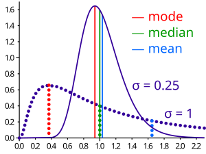
Geometric visualization of the mode, median and mean of an arbitrary probability density function[9]
For any real-valued probability distribution with cumulative distribution function F, a median is defined as any real number m that satisfies the inequalities
![{displaystyle int _{(-infty ,m]}dF(x)geq {frac {1}{2}}{text{ and }}int _{[m,infty )}dF(x)geq {frac {1}{2}}.}](https://wikimedia.org/api/rest_v1/media/math/render/svg/6f38cd2176b48f55c51f4ce62dd514aac773273f)
An equivalent phrasing uses a random variable X distributed according to F:

Note that this definition does not require X to have an absolutely continuous distribution (which has a probability density function f), nor does it require a discrete one. In the former case, the inequalities can be upgraded to equality: a median satisfies

Any probability distribution on R has at least one median, but in pathological cases there may be more than one median: if F is constant 1/2 on an interval (so that f=0 there), then any value of that interval is a median.
Medians of particular distributions[edit]
The medians of certain types of distributions can be easily calculated from their parameters; furthermore, they exist even for some distributions lacking a well-defined mean, such as the Cauchy distribution:
- The median of a symmetric unimodal distribution coincides with the mode.
- The median of a symmetric distribution which possesses a mean μ also takes the value μ.
- The median of a normal distribution with mean μ and variance σ2 is μ. In fact, for a normal distribution, mean = median = mode.
- The median of a uniform distribution in the interval [a, b] is (a + b) / 2, which is also the mean.
- The median of a Cauchy distribution with location parameter x0 and scale parameter y is x0, the location parameter.
- The median of a power law distribution x−a, with exponent a > 1 is 21/(a − 1)xmin, where xmin is the minimum value for which the power law holds[10]
- The median of an exponential distribution with rate parameter λ is the natural logarithm of 2 divided by the rate parameter: λ−1ln 2.
- The median of a Weibull distribution with shape parameter k and scale parameter λ is λ(ln 2)1/k.
Properties[edit]
Optimality property[edit]
The mean absolute error of a real variable c with respect to the random variable X is

Provided that the probability distribution of X is such that the above expectation exists, then m is a median of X if and only if m is a minimizer of the mean absolute error with respect to X.[11] In particular, m is a sample median if and only if m minimizes the arithmetic mean of the absolute deviations.[12]
More generally, a median is defined as a minimum of

as discussed below in the section on multivariate medians (specifically, the spatial median).
This optimization-based definition of the median is useful in statistical data-analysis, for example, in k-medians clustering.
Inequality relating means and medians[edit]
If the distribution has finite variance, then the distance between the median  and the mean
  is bounded by one standard deviation.
This bound was proved by Book and Sher in 1979 for discrete samples,[13] and more generally by Page and Murty in 1982.[14] In a comment on a subsequent proof by O’Cinneide,[15] Mallows in 1991 presented a compact proof that uses Jensen’s inequality twice,[16] as follows. Using |·| for the absolute value, we have

The first and third inequalities come from Jensen’s inequality applied to the absolute-value function and the square function, which are each convex. The second inequality comes from the fact that a median minimizes the absolute deviation function  .
.
Mallows’s proof can be generalized to obtain a multivariate version of the inequality[17] simply by replacing the absolute value with a norm:

where m is a spatial median, that is, a minimizer of the function  The spatial median is unique when the data-set’s dimension is two or more.[18][19]
An alternative proof uses the one-sided Chebyshev inequality; it appears in an inequality on location and scale parameters. This formula also follows directly from Cantelli’s inequality.[20]
Unimodal distributions[edit]
For the case of unimodal distributions, one can achieve a sharper bound on the distance between the median and the mean:
- .[21]

A similar relation holds between the median and the mode:

Jensen’s inequality for medians[edit]
Jensen’s inequality states that for any random variable X with a finite expectation E[X] and for any convex function f
![{displaystyle f[E(x)]leq E[f(x)]}](https://wikimedia.org/api/rest_v1/media/math/render/svg/1874d0eeb97b95fcab3c70f25df212e2cb4af2d2)
This inequality generalizes to the median as well. We say a function f: R → R is a C function if, for any t,
![{displaystyle f^{-1}left(,(-infty ,t],right)={xin mathbb {R} mid f(x)leq t}}](https://wikimedia.org/api/rest_v1/media/math/render/svg/0bb6a4a02d8480c441a0f73bea93cc4fffb9b08d)
is a closed interval (allowing the degenerate cases of a single point or an empty set). Every convex function is a C function, but the reverse does not hold. If f is a C function, then
![{displaystyle f(operatorname {Median} [X])leq operatorname {Median} [f(X)]}](https://wikimedia.org/api/rest_v1/media/math/render/svg/71d1c1e4434b41fe5617b85c49b2e9d308c8a1a3)
If the medians are not unique, the statement holds for the corresponding suprema.[22]
Medians for samples[edit]
This section discusses the theory of estimating a population median from a sample. To calculate the median of a sample «by hand,» see § Finite data set of numbers above.
The sample median[edit]
Efficient computation of the sample median[edit]
Even though comparison-sorting n items requires Ω(n log n) operations, selection algorithms can compute the kth-smallest of n items with only Θ(n) operations. This includes the median, which is the n/2th order statistic (or for an even number of samples, the arithmetic mean of the two middle order statistics).[23]
Selection algorithms still have the downside of requiring Ω(n) memory, that is, they need to have the full sample (or a linear-sized portion of it) in memory. Because this, as well as the linear time requirement, can be prohibitive, several estimation procedures for the median have been developed. A simple one is the median of three rule, which estimates the median as the median of a three-element subsample; this is commonly used as a subroutine in the quicksort sorting algorithm, which uses an estimate of its input’s median. A more robust estimator is Tukey’s ninther, which is the median of three rule applied with limited recursion:[24] if A is the sample laid out as an array, and
- med3(A) = median(A[1], A[n/2], A[n]),
then
- ninther(A) = med3(med3(A[1 … 1/3n]), med3(A[1/3n … 2/3n]), med3(A[2/3n … n]))
The remedian is an estimator for the median that requires linear time but sub-linear memory, operating in a single pass over the sample.[25]
Sampling distribution[edit]
The distributions of both the sample mean and the sample median were determined by Laplace.[26] The distribution of the sample median from a population with a density function  is asymptotically normal with mean
  and variance[27]

where  is the median of and is the sample size. A modern proof follows below. Laplace’s result is now understood as a special case of the asymptotic distribution of arbitrary quantiles.
For normal samples, the density is  , thus for large samples the variance of the median equals
  [7] (See also section #Efficiency below.)
Derivation of the asymptotic distribution[edit]
We take the sample size to be an odd number  and assume our variable continuous; the formula for the case of discrete variables is given below in § Empirical local density. The sample can be summarized as «below median», «at median», and «above median», which corresponds to a trinomial distribution with probabilities
  ,
,  and
and  . For a continuous variable, the probability of multiple sample values being exactly equal to the median is 0, so one can calculate the density of at the point
  directly from the trinomial distribution:
- .
![{displaystyle Pr[operatorname {Median} =v],dv={frac {(2n+1)!}{n!n!}}F(v)^{n}(1-F(v))^{n}f(v),dv}](https://wikimedia.org/api/rest_v1/media/math/render/svg/b99f214189b2882487bfbae7997046efa4a88cc4)
Now we introduce the beta function. For integer arguments  and
and  , this can be expressed as
  . Also, recall that
  . Using these relationships and setting both and equal to
  allows the last expression to be written as

Hence the density function of the median is a symmetric beta distribution pushed forward by  . Its mean, as we would expect, is 0.5 and its variance is
  . By the chain rule, the corresponding variance of the sample median is
- .

The additional 2 is negligible in the limit.
Empirical local density[edit]
In practice, the functions  and are often not known or assumed. However, they can be estimated from an observed frequency distribution. In this section, we give an example. Consider the following table, representing a sample of 3,800 (discrete-valued) observations:
| v | 0 | 0.5 | 1 | 1.5 | 2 | 2.5 | 3 | 3.5 | 4 | 4.5 | 5 |
|---|---|---|---|---|---|---|---|---|---|---|---|
| f(v) | 0.000 | 0.008 | 0.010 | 0.013 | 0.083 | 0.108 | 0.328 | 0.220 | 0.202 | 0.023 | 0.005 |
| F(v) | 0.000 | 0.008 | 0.018 | 0.031 | 0.114 | 0.222 | 0.550 | 0.770 | 0.972 | 0.995 | 1.000 |
Because the observations are discrete-valued, constructing the exact distribution of the median is not an immediate translation of the above expression for  ; one may (and typically does) have multiple instances of the median in one’s sample. So we must sum over all these possibilities:

Here, i is the number of points strictly less than the median and k the number strictly greater.
Using these preliminaries, it is possible to investigate the effect of sample size on the standard errors of the mean and median. The observed mean is 3.16, the observed raw median is 3 and the observed interpolated median is 3.174. The following table gives some comparison statistics.
|
Sample size Statistic |
3 | 9 | 15 | 21 |
|---|---|---|---|---|
| Expected value of median | 3.198 | 3.191 | 3.174 | 3.161 |
| Standard error of median (above formula) | 0.482 | 0.305 | 0.257 | 0.239 |
| Standard error of median (asymptotic approximation) | 0.879 | 0.508 | 0.393 | 0.332 |
| Standard error of mean | 0.421 | 0.243 | 0.188 | 0.159 |
The expected value of the median falls slightly as sample size increases while, as would be expected, the standard errors of both the median and the mean are proportionate to the inverse square root of the sample size. The asymptotic approximation errs on the side of caution by overestimating the standard error.
Estimation of variance from sample data[edit]
The value of  —the asymptotic value of
  where
where  is the population median—has been studied by several authors. The standard «delete one» jackknife method produces inconsistent results.[28] An alternative—the «delete k» method—where
  grows with the sample size has been shown to be asymptotically consistent.[29] This method may be computationally expensive for large data sets. A bootstrap estimate is known to be consistent,[30] but converges very slowly (order of
  ).[31] Other methods have been proposed but their behavior may differ between large and small samples.[32]
Efficiency[edit]
The efficiency of the sample median, measured as the ratio of the variance of the mean to the variance of the median, depends on the sample size and on the underlying population distribution. For a sample of size from the normal distribution, the efficiency for large N is

The efficiency tends to  as
as  tends to infinity.
In other words, the relative variance of the median will be  , or 57% greater than the variance of the mean – the relative standard error of the median will be
  , or 25% greater than the standard error of the mean,
  (see also section #Sampling distribution above.).[33]
Other estimators[edit]
For univariate distributions that are symmetric about one median, the Hodges–Lehmann estimator is a robust and highly efficient estimator of the population median.[34]
If data is represented by a statistical model specifying a particular family of probability distributions, then estimates of the median can be obtained by fitting that family of probability distributions to the data and calculating the theoretical median of the fitted distribution.[citation needed] Pareto interpolation is an application of this when the population is assumed to have a Pareto distribution.
Multivariate median[edit]
Previously, this article discussed the univariate median, when the sample or population had one-dimension. When the dimension is two or higher, there are multiple concepts that extend the definition of the univariate median; each such multivariate median agrees with the univariate median when the dimension is exactly one.[34][35][36][37]
Marginal median[edit]
The marginal median is defined for vectors defined with respect to a fixed set of coordinates. A marginal median is defined to be the vector whose components are univariate medians. The marginal median is easy to compute, and its properties were studied by Puri and Sen.[34][38]
Geometric median[edit]
The geometric median of a discrete set of sample points  in a Euclidean space is the[a] point minimizing the sum of distances to the sample points.

In contrast to the marginal median, the geometric median is equivariant with respect to Euclidean similarity transformations such as translations and rotations.
Median in all directions[edit]
If the marginal medians for all coordinate systems coincide, then their common location may be termed the «median in all directions».[40] This concept is relevant to voting theory on account of the median voter theorem. When it exists, the median in all directions coincides with the geometric median (at least for discrete distributions).
Centerpoint[edit]
An alternative generalization of the median in higher dimensions is the centerpoint.
[edit]
Interpolated median[edit]
When dealing with a discrete variable, it is sometimes useful to regard the observed values as being midpoints of underlying continuous intervals. An example of this is a Likert scale, on which opinions or preferences are expressed on a scale with a set number of possible responses. If the scale consists of the positive integers, an observation of 3 might be regarded as representing the interval from 2.50 to 3.50. It is possible to estimate the median of the underlying variable. If, say, 22% of the observations are of value 2 or below and 55.0% are of 3 or below (so 33% have the value 3), then the median is 3 since the median is the smallest value of for which  is greater than a half. But the interpolated median is somewhere between 2.50 and 3.50. First we add half of the interval width
  to the median to get the upper bound of the median interval. Then we subtract that proportion of the interval width which equals the proportion of the 33% which lies above the 50% mark. In other words, we split up the interval width pro rata to the numbers of observations. In this case, the 33% is split into 28% below the median and 5% above it so we subtract 5/33 of the interval width from the upper bound of 3.50 to give an interpolated median of 3.35. More formally, if the values are known, the interpolated median can be calculated from
![{displaystyle m_{text{int}}=m+wleft[{frac {1}{2}}-{frac {F(m)-{frac {1}{2}}}{f(m)}}right].}](https://wikimedia.org/api/rest_v1/media/math/render/svg/5e823608d9eba650d4796825d3043ef41d06370e)
Alternatively, if in an observed sample there are scores above the median category,  scores in it and
  scores below it then the interpolated median is given by
![{displaystyle m_{text{int}}=m+{frac {w}{2}}left[{frac {k-i}{j}}right].}](https://wikimedia.org/api/rest_v1/media/math/render/svg/8519008345d5bd2863ff18203d1b6144f851ae95)
Pseudo-median[edit]
For univariate distributions that are symmetric about one median, the Hodges–Lehmann estimator is a robust and highly efficient estimator of the population median; for non-symmetric distributions, the Hodges–Lehmann estimator is a robust and highly efficient estimator of the population pseudo-median, which is the median of a symmetrized distribution and which is close to the population median.[41] The Hodges–Lehmann estimator has been generalized to multivariate distributions.[42]
Variants of regression[edit]
The Theil–Sen estimator is a method for robust linear regression based on finding medians of slopes.[43]
Median filter[edit]
The median filter is an important tool of image processing, that can effectively remove any salt and pepper noise from grayscale images.
Cluster analysis[edit]
In cluster analysis, the k-medians clustering algorithm provides a way of defining clusters, in which the criterion of maximising the distance between cluster-means that is used in k-means clustering, is replaced by maximising the distance between cluster-medians.
Median–median line[edit]
This is a method of robust regression. The idea dates back to Wald in 1940 who suggested dividing a set of bivariate data into two halves depending on the value of the independent parameter : a left half with values less than the median and a right half with values greater than the median.[44] He suggested taking the means of the dependent  and independent variables of the left and the right halves and estimating the slope of the line joining these two points. The line could then be adjusted to fit the majority of the points in the data set.
Nair and Shrivastava in 1942 suggested a similar idea but instead advocated dividing the sample into three equal parts before calculating the means of the subsamples.[45] Brown and Mood in 1951 proposed the idea of using the medians of two subsamples rather the means.[46] Tukey combined these ideas and recommended dividing the sample into three equal size subsamples and estimating the line based on the medians of the subsamples.[47]
Median-unbiased estimators[edit]
Any mean-unbiased estimator minimizes the risk (expected loss) with respect to the squared-error loss function, as observed by Gauss. A median-unbiased estimator minimizes the risk with respect to the absolute-deviation loss function, as observed by Laplace. Other loss functions are used in statistical theory, particularly in robust statistics.
The theory of median-unbiased estimators was revived by George W. Brown in 1947:[48]
An estimate of a one-dimensional parameter θ will be said to be median-unbiased if, for fixed θ, the median of the distribution of the estimate is at the value θ; i.e., the estimate underestimates just as often as it overestimates. This requirement seems for most purposes to accomplish as much as the mean-unbiased requirement and has the additional property that it is invariant under one-to-one transformation.
— page 584
Further properties of median-unbiased estimators have been reported.[49][50][51][52] Median-unbiased estimators are invariant under one-to-one transformations.
There are methods of constructing median-unbiased estimators that are optimal (in a sense analogous to the minimum-variance property for mean-unbiased estimators). Such constructions exist for probability distributions having monotone likelihood-functions.[53][54] One such procedure is an analogue of the Rao–Blackwell procedure for mean-unbiased estimators: The procedure holds for a smaller class of probability distributions than does the Rao—Blackwell procedure but for a larger class of loss functions.[55]
History[edit]
Scientific researchers in the ancient near east appear not to have used summary statistics altogether, instead choosing values that offered maximal consistency with a broader theory that integrated a wide variety of phenomena.[56] Within the Mediterranean (and, later, European) scholarly community, statistics like the mean are fundamentally a medieval and early modern development. (The history of the median outside Europe and its predecessors remains relatively unstudied.)
The idea of the median appeared in the 6th century in the Talmud, in order to fairly analyze divergent appraisals.[57][58] However, the concept did not spread to the broader scientific community.
Instead, the closest ancestor of the modern median is the mid-range, invented by Al-Biruni.[59]: 31 [60] Transmission of Al-Biruni’s work to later scholars is unclear. Al-Biruni applied his technique to assaying metals, but, after he published his work, most assayers still adopted the most unfavorable value from their results, lest they appear to cheat.[59]: 35–8 However, increased navigation at sea during the Age of Discovery meant that ship’s navigators increasingly had to attempt to determine latitude in unfavorable weather against hostile shores, leading to renewed interest in summary statistics. Whether rediscovered or independently invented, the mid-range is recommended to nautical navigators in Harriot’s «Instructions for Raleigh’s Voyage to Guiana, 1595».[59]: 45–8
The idea of the median may have first appeared in Edward Wright’s 1599 book Certaine Errors in Navigation on a section about compass navigation. Wright was reluctant to discard measured values, and may have felt that the median — incorporating a greater proportion of the dataset than the mid-range — was more likely to be correct. However, Wright did not give examples of his technique’s use, making it hard to verify that he described the modern notion of median.[56][60][b] The median (in the context of probability) certainly appeared in the correspondence of Christiaan Huygens, but as an example of a statistic that was inappropriate for actuarial practice.[56]
The earliest recommendation of the median dates to 1757, when Roger Joseph Boscovich developed a regression method based on the L1 norm and therefore implicitly on the median.[56][61] In 1774, Laplace made this desire explicit: he suggested the median be used as the standard estimator of the value of a posterior PDF. The specific criterion was to minimize the expected magnitude of the error;  where
where  is the estimate and is the true value. To this end, Laplace determined the distributions of both the sample mean and the sample median in the early 1800s.[26][62] However, a decade later, Gauss and Legendre developed the least squares method, which minimizes
  to obtain the mean. Within the context of regression, Gauss and Legendre’s innovation offers vastly easier computation. Consequently, Laplaces’ proposal was generally rejected until the rise of computing devices 150 years later (and is still a relatively uncommon algorithm).[63]
Antoine Augustin Cournot in 1843 was the first[64] to use the term median (valeur médiane) for the value that divides a probability distribution into two equal halves. Gustav Theodor Fechner used the median (Centralwerth) in sociological and psychological phenomena.[65] It had earlier been used only in astronomy and related fields. Gustav Fechner popularized the median into the formal analysis of data, although it had been used previously by Laplace,[65] and the median appeared in a textbook by F. Y. Edgeworth.[66] Francis Galton used the English term median in 1881,[67][68] having earlier used the terms middle-most value in 1869, and the medium in 1880.[69][70]
Statisticians encouraged the use of medians intensely throughout the 19th century for its intuitive clarity and ease of manual computation. However, the notion of median does not lend itself to the theory of higher moments as well as the arithmetic mean does, and is much harder to compute by computer. As a result, the median was steadily supplanted as a notion of generic average by the arithmetic mean during the 20th century.[56][60]
See also[edit]
- Absolute deviation
- Bias of an estimator
- Central tendency
- Concentration of measure for Lipschitz functions
- Median graph
- Median of medians – Algorithm to calculate the approximate median in linear time
- Median search
- Median slope
- Median voter theory
- Medoids – Generalization of the median in higher dimensions
Notes[edit]
- ^ The geometric median is unique unless the sample is collinear.[39]
- ^ Subsequent scholars appear to concur with Eisenhart that Boroughs’ 1580 figures, while suggestive of the median, in fact describe an arithmetic mean.;[59]: 62–3 Boroughs is mentioned in no other work.
References[edit]
- ^ a b Weisstein, Eric W. «Statistical Median». MathWorld.
- ^ Simon, Laura J.; «Descriptive statistics» Archived 2010-07-30 at the Wayback Machine, Statistical Education Resource Kit, Pennsylvania State Department of Statistics
- ^ David J. Sheskin (27 August 2003). Handbook of Parametric and Nonparametric Statistical Procedures (Third ed.). CRC Press. pp. 7–. ISBN 978-1-4200-3626-8. Retrieved 25 February 2013.
- ^ Derek Bissell (1994). Statistical Methods for Spc and Tqm. CRC Press. pp. 26–. ISBN 978-0-412-39440-9. Retrieved 25 February 2013.
- ^ Paul T. von Hippel (2005). «Mean, Median, and Skew: Correcting a Textbook Rule». Journal of Statistics Education. 13 (2). Archived from the original on 2008-10-14. Retrieved 2015-06-18.
- ^ Robson, Colin (1994). Experiment, Design and Statistics in Psychology. Penguin. pp. 42–45. ISBN 0-14-017648-9.
- ^ a b Williams, D. (2001). Weighing the Odds. Cambridge University Press. p. 165. ISBN 052100618X.
- ^ Maindonald, John; Braun, W. John (2010-05-06). Data Analysis and Graphics Using R: An Example-Based Approach. Cambridge University Press. p. 104. ISBN 978-1-139-48667-5.
- ^ «AP Statistics Review — Density Curves and the Normal Distributions». Archived from the original on 8 April 2015. Retrieved 16 March 2015.
- ^ Newman, Mark EJ. «Power laws, Pareto distributions and Zipf’s law.» Contemporary physics 46.5 (2005): 323–351.
- ^ Stroock, Daniel (2011). Probability Theory. Cambridge University Press. pp. 43. ISBN 978-0-521-13250-3.
- ^ André Nicolas (https://math.stackexchange.com/users/6312/andr%c3%a9-nicolas), The Median Minimizes the Sum of Absolute Deviations (The $ {L}_{1} $ Norm), URL (version: 2012-02-25): https://math.stackexchange.com/q/113336
- ^ Stephen A. Book; Lawrence Sher (1979). «How close are the mean and the median?». The Two-Year College Mathematics Journal. 10 (3): 202–204. doi:10.2307/3026748. JSTOR 3026748. Retrieved 12 March 2022.
- ^ Warren Page; Vedula N. Murty (1982). «Nearness Relations Among Measures of Central Tendency and Dispersion: Part 1». The Two-Year College Mathematics Journal. 13 (5): 315–327. doi:10.1080/00494925.1982.11972639 (inactive 31 December 2022). Retrieved 12 March 2022.
{{cite journal}}: CS1 maint: DOI inactive as of December 2022 (link) - ^ O’Cinneide, Colm Art (1990). «The mean is within one standard deviation of any median». The American Statistician. 44 (4): 292–293. doi:10.1080/00031305.1990.10475743. Retrieved 12 March 2022.
- ^ Mallows, Colin (August 1991). «Another comment on O’Cinneide». The American Statistician. 45 (3): 257. doi:10.1080/00031305.1991.10475815.
- ^ Piché, Robert (2012). Random Vectors and Random Sequences. Lambert Academic Publishing. ISBN 978-3659211966.
- ^ Kemperman, Johannes H. B. (1987). Dodge, Yadolah (ed.). «The median of a finite measure on a Banach space: Statistical data analysis based on the L1-norm and related methods». Papers from the First International Conference Held at Neuchâtel, August 31–September 4, 1987. Amsterdam: North-Holland Publishing Co.: 217–230. MR 0949228.
- ^ Milasevic, Philip; Ducharme, Gilles R. (1987). «Uniqueness of the spatial median». Annals of Statistics. 15 (3): 1332–1333. doi:10.1214/aos/1176350511. MR 0902264.
- ^ K.Van Steen Notes on probability and statistics
- ^ Basu, S.; Dasgupta, A. (1997). «The Mean, Median, and Mode of Unimodal Distributions:A Characterization». Theory of Probability and Its Applications. 41 (2): 210–223. doi:10.1137/S0040585X97975447. S2CID 54593178.
- ^ Merkle, M. (2005). «Jensen’s inequality for medians». Statistics & Probability Letters. 71 (3): 277–281. doi:10.1016/j.spl.2004.11.010.
- ^ Alfred V. Aho and John E. Hopcroft and Jeffrey D. Ullman (1974). The Design and Analysis of Computer Algorithms. Reading/MA: Addison-Wesley. ISBN 0-201-00029-6. Here: Section 3.6 «Order Statistics», p.97-99, in particular Algorithm 3.6 and Theorem 3.9.
- ^ Bentley, Jon L.; McIlroy, M. Douglas (1993). «Engineering a sort function». Software: Practice and Experience. 23 (11): 1249–1265. doi:10.1002/spe.4380231105. S2CID 8822797.
- ^ Rousseeuw, Peter J.; Bassett, Gilbert W. Jr. (1990). «The remedian: a robust averaging method for large data sets» (PDF). J. Amer. Statist. Assoc. 85 (409): 97–104. doi:10.1080/01621459.1990.10475311.
- ^ a b Stigler, Stephen (December 1973). «Studies in the History of Probability and Statistics. XXXII: Laplace, Fisher and the Discovery of the Concept of Sufficiency». Biometrika. 60 (3): 439–445. doi:10.1093/biomet/60.3.439. JSTOR 2334992. MR 0326872.
- ^ Rider, Paul R. (1960). «Variance of the median of small samples from several special populations». J. Amer. Statist. Assoc. 55 (289): 148–150. doi:10.1080/01621459.1960.10482056.
- ^ Efron, B. (1982). The Jackknife, the Bootstrap and other Resampling Plans. Philadelphia: SIAM. ISBN 0898711797.
- ^ Shao, J.; Wu, C. F. (1989). «A General Theory for Jackknife Variance Estimation». Ann. Stat. 17 (3): 1176–1197. doi:10.1214/aos/1176347263. JSTOR 2241717.
- ^ Efron, B. (1979). «Bootstrap Methods: Another Look at the Jackknife». Ann. Stat. 7 (1): 1–26. doi:10.1214/aos/1176344552. JSTOR 2958830.
- ^ Hall, P.; Martin, M. A. (1988). «Exact Convergence Rate of Bootstrap Quantile Variance Estimator». Probab Theory Related Fields. 80 (2): 261–268. doi:10.1007/BF00356105. S2CID 119701556.
- ^ Jiménez-Gamero, M. D.; Munoz-García, J.; Pino-Mejías, R. (2004). «Reduced bootstrap for the median». Statistica Sinica. 14 (4): 1179–1198.
- ^ Maindonald, John; John Braun, W. (2010-05-06). Data Analysis and Graphics Using R: An Example-Based Approach. ISBN 9781139486675.
- ^ a b c Hettmansperger, Thomas P.; McKean, Joseph W. (1998). Robust nonparametric statistical methods. Kendall’s Library of Statistics. Vol. 5. London: Edward Arnold. ISBN 0-340-54937-8. MR 1604954.
- ^ Small, Christopher G. «A survey of multidimensional medians.» International Statistical Review/Revue Internationale de Statistique (1990): 263–277. doi:10.2307/1403809 JSTOR 1403809
- ^ Niinimaa, A., and H. Oja. «Multivariate median.» Encyclopedia of statistical sciences (1999).
- ^ Mosler, Karl. Multivariate Dispersion, Central Regions, and Depth: The Lift Zonoid Approach. Vol. 165. Springer Science & Business Media, 2012.
- ^ Puri, Madan L.; Sen, Pranab K.; Nonparametric Methods in Multivariate Analysis, John Wiley & Sons, New York, NY, 1971. (Reprinted by Krieger Publishing)
- ^ Vardi, Yehuda; Zhang, Cun-Hui (2000). «The multivariate L1-median and associated data depth». Proceedings of the National Academy of Sciences of the United States of America. 97 (4): 1423–1426 (electronic). Bibcode:2000PNAS…97.1423V. doi:10.1073/pnas.97.4.1423. MR 1740461. PMC 26449. PMID 10677477.
- ^ Davis, Otto A.; DeGroot, Morris H.; Hinich, Melvin J. (January 1972). «Social Preference Orderings and Majority Rule» (PDF). Econometrica. 40 (1): 147–157. doi:10.2307/1909727. JSTOR 1909727. The authors, working in a topic in which uniqueness is assumed, actually use the expression «unique median in all directions».
- ^ Pratt, William K.; Cooper, Ted J.; Kabir, Ihtisham (1985-07-11). Corbett, Francis J (ed.). «Pseudomedian Filter». Architectures and Algorithms for Digital Image Processing II. 0534: 34. Bibcode:1985SPIE..534…34P. doi:10.1117/12.946562. S2CID 173183609.
- ^ Oja, Hannu (2010). Multivariate nonparametric methods with R: An approach based on spatial signs and ranks. Lecture Notes in Statistics. Vol. 199. New York, NY: Springer. pp. xiv+232. doi:10.1007/978-1-4419-0468-3. ISBN 978-1-4419-0467-6. MR 2598854.
- ^ Wilcox, Rand R. (2001), «Theil–Sen estimator», Fundamentals of Modern Statistical Methods: Substantially Improving Power and Accuracy, Springer-Verlag, pp. 207–210, ISBN 978-0-387-95157-7.
- ^ Wald, A. (1940). «The Fitting of Straight Lines if Both Variables are Subject to Error» (PDF). Annals of Mathematical Statistics. 11 (3): 282–300. doi:10.1214/aoms/1177731868. JSTOR 2235677.
- ^ Nair, K. R.; Shrivastava, M. P. (1942). «On a Simple Method of Curve Fitting». Sankhyā: The Indian Journal of Statistics. 6 (2): 121–132. JSTOR 25047749.
- ^ Brown, G. W.; Mood, A. M. (1951). «On Median Tests for Linear Hypotheses». Proc Second Berkeley Symposium on Mathematical Statistics and Probability. Berkeley, CA: University of California Press. pp. 159–166. Zbl 0045.08606.
- ^ Tukey, J. W. (1977). Exploratory Data Analysis. Reading, MA: Addison-Wesley. ISBN 0201076160.
- ^ Brown, George W. (1947). «On Small-Sample Estimation». Annals of Mathematical Statistics. 18 (4): 582–585. doi:10.1214/aoms/1177730349. JSTOR 2236236.
- ^ Lehmann, Erich L. (1951). «A General Concept of Unbiasedness». Annals of Mathematical Statistics. 22 (4): 587–592. doi:10.1214/aoms/1177729549. JSTOR 2236928.
- ^ Birnbaum, Allan (1961). «A Unified Theory of Estimation, I». Annals of Mathematical Statistics. 32 (1): 112–135. doi:10.1214/aoms/1177705145. JSTOR 2237612.
- ^ van der Vaart, H. Robert (1961). «Some Extensions of the Idea of Bias». Annals of Mathematical Statistics. 32 (2): 436–447. doi:10.1214/aoms/1177705051. JSTOR 2237754. MR 0125674.
- ^ Pfanzagl, Johann; with the assistance of R. Hamböker (1994). Parametric Statistical Theory. Walter de Gruyter. ISBN 3-11-013863-8. MR 1291393.
- ^ Pfanzagl, Johann. «On optimal median unbiased estimators in the presence of nuisance parameters.» The Annals of Statistics (1979): 187–193.
- ^ Brown, L. D.; Cohen, Arthur; Strawderman, W. E. (1976). «A Complete Class Theorem for Strict Monotone Likelihood Ratio With Applications». Ann. Statist. 4 (4): 712–722. doi:10.1214/aos/1176343543.
- ^ Page; Brown, L. D.; Cohen, Arthur; Strawderman, W. E. (1976). «A Complete Class Theorem for Strict Monotone Likelihood Ratio With Applications». Ann. Statist. 4 (4): 712–722. doi:10.1214/aos/1176343543.
- ^ a b c d e Bakker, Arthur; Gravemeijer, Koeno P. E. (2006-06-01). «An Historical Phenomenology of Mean and Median». Educational Studies in Mathematics. 62 (2): 149–168. doi:10.1007/s10649-006-7099-8. ISSN 1573-0816. S2CID 143708116.
- ^ Adler, Dan (31 December 2014). «Talmud and Modern Economics». Jewish American and Israeli Issues. Archived from the original on 6 December 2015. Retrieved 22 February 2020.
- ^ Modern Economic Theory in the Talmud by Yisrael Aumann
- ^ a b c d Eisenhart, Churchill (24 August 1971). The Development of the Concept of the Best Mean of a Set of Measurements from Antiquity to the Present Day (PDF) (Speech). 131st Annual Meeting of the American Statistical Association. Colorado State University.
- ^ a b c «How the Average Triumphed Over the Median». Priceonomics. 5 April 2016. Retrieved 2020-02-23.
- ^ Stigler, S. M. (1986). The History of Statistics: The Measurement of Uncertainty Before 1900. Harvard University Press. ISBN 0674403401.
- ^ Laplace PS de (1818) Deuxième supplément à la Théorie Analytique des Probabilités, Paris, Courcier
- ^ Jaynes, E.T. (2007). Probability theory : the logic of science (5. print. ed.). Cambridge [u.a.]: Cambridge Univ. Press. p. 172. ISBN 978-0-521-59271-0.
- ^ Howarth, Richard (2017). Dictionary of Mathematical Geosciences: With Historical Notes. Springer. p. 374.
- ^ a b Keynes, J.M. (1921) A Treatise on Probability. Pt II Ch XVII §5 (p 201) (2006 reprint, Cosimo Classics, ISBN 9781596055308 : multiple other reprints)
- ^ Stigler, Stephen M. (2002). Statistics on the Table: The History of Statistical Concepts and Methods. Harvard University Press. pp. 105–7. ISBN 978-0-674-00979-0.
- ^ Galton F (1881) «Report of the Anthropometric Committee» pp 245–260. Report of the 51st Meeting of the British Association for the Advancement of Science
- ^ David, H. A. (1995). «First (?) Occurrence of Common Terms in Mathematical Statistics». The American Statistician. 49 (2): 121–133. doi:10.2307/2684625. ISSN 0003-1305. JSTOR 2684625.
- ^ encyclopediaofmath.org
- ^ personal.psu.edu
External links[edit]
- «Median (in statistics)», Encyclopedia of Mathematics, EMS Press, 2001 [1994]
- Median as a weighted arithmetic mean of all Sample Observations
- On-line calculator
- Calculating the median
- A problem involving the mean, the median, and the mode.
- Weisstein, Eric W. «Statistical Median». MathWorld.
- Python script for Median computations and income inequality metrics
- Fast Computation of the Median by Successive Binning
- ‘Mean, median, mode and skewness’, A tutorial devised for first-year psychology students at Oxford University, based on a worked example.
- The Complex SAT Math Problem Even the College Board Got Wrong: Andrew Daniels in Popular Mechanics
This article incorporates material from Median of a distribution on PlanetMath, which is licensed under the Creative Commons Attribution/Share-Alike License.
Время прочтения
9 мин
Просмотры 6.7K
Предыдущий пост см. здесь.
Выборки и популяции
В статистической науке термины «выборка» и «популяция» имеют особое значение. Популяция, или генеральная совокупность, — это все множество объектов, которые исследователь хочет понять или в отношении которых сделать выводы. Например, во второй половине 19-го века основоположник генетики Грегор Йохан Мендель) записывал наблюдения о растениях гороха. Несмотря на то, что он изучал в лабораторных условиях вполне конкретные сорта растения, его задача состояла в том, чтобы понять базовые механизмы, лежащие в основе наследственности абсолютно всех возможных сортов гороха.
В статистической науке о группе объектов, из которых извлекается выборка, говорят, как о популяции, независимо от того, являются изучаемые объекты живыми существами или нет.
Поскольку популяция может быть крупной — или бесконечной, как в случае растений гороха Менделя — мы должны изучать репрезентативные выборки, и на их основе делать выводы о всей популяции в целом. В целях проведения четкого различия между поддающимися измерению атрибутами выборок и недоступными атрибутами популяции, мы используем термин статистики, имея при этом в виду атрибуты выборки, и говорим о параметрах, имея в виду атрибуты популяции.
Статистики — это атрибуты, которые мы можем измерить на основе выборок. Параметры — это атрибуты популяции, которые мы пытаемся вывести статистически.
В действительности, статистики и параметры различаются в силу применения разных символов в математических формулах:
|
Мера |
Выборочная статистика |
Популяционный параметр |
|
Объем |
n |
N |
|
Среднее значение |
x̅ |
μx |
|
Стандартное отклонение |
Sx |
σx |
|
Стандартная ошибка |
Sx̅ |
Если вы вернетесь к уравнению стандартной ошибки, то заметите, что она вычисляется не из выборочного стандартного отклонения Sx, а из популяционного стандартного отклонения σx. Это создает парадоксальную ситуацию — мы не можем вычислить выборочную статистику, используя для этого популяционные параметры, которые мы пытаемся вывести. На практике, однако, предполагается, что выборочное и популяционное стандартные отклонения одинаковы при размере выборки порядка n ≥ 30.
Теперь вычислим стандартную ошибку средних значений за определенный день. Например, возьмем конкретный день, скажем, 1 мая:
def ex_2_8():
    '''Вычислить стандартную ошибку
       средних значений за определенный день'''
    may_1 = '2015-05-01'
    df = with_parsed_date( load_data('dwell-times.tsv') )
    filtered = df.set_index( ['date'] )[may_1]
    se = standard_error( filtered['dwell-time'] )
    print('Стандартная ошибка:', se)
Стандартная ошибка: 3.627340273094217Хотя мы взяли выборку всего из одного дня, вычисляемая нами стандартная ошибка очень близка к стандартному отклонению всех выборочных средних — 3.6 сек. против 3.7 сек. Это, как если бы, подобно клетке, содержащей ДНК, в каждой выборке была закодирована информация обо всей находящейся внутри нее популяции.
Интервалы уверенности
Поскольку стандартная ошибка выборки измеряет степень близости, с которой, по нашим ожиданиям, выборочное среднее соответствует среднему популяционному, то мы можем также рассмотреть обратное — стандартная ошибка измеряет степень близосто, с которой, по нашим ожиданиям, популяционное среднее соответствует измеренному среднему выборочному. Другими словами, на основе стандартной ошибки мы можем вывести, что популяционное среднее находится в пределах некого ожидаемого диапазона выборочного среднего с некоторой степенью уверенности.
Понятия «степень уверенности» и «ожидаемый диапазон», взятые вместе, дают определение термину интервал уверенности.
Примечание. В большинстве языков под термином «confidence» в контексте инференциальной статистики понимается именно уверенность в отличие от отечественной статистики, где принято говорить о доверительном интервале. На самом деле речь идет не о доверии (trust), а об уверенности исследователя в полученных результатах. Это яркий пример мягкой подмены понятия. Подобного рода ошибки вполне объяснимы — первые переводы появились еще в
доколумбовудоинтернетовскую эпоху, когда источников было мало, и приходилось домысливать в силу своего понимания. Сегодня же, когда существует масса профильных глоссариев, словарей и источников, такого рода искажения не оправданы. ИМХО.
При установлении интервалов уверенности обычной практикой является задание интервала размером 95% — мы на 95% уверены, что популяционный параметр находится внутри интервала. Разумеется, еще остается 5%-я возможность, что он там не находится.
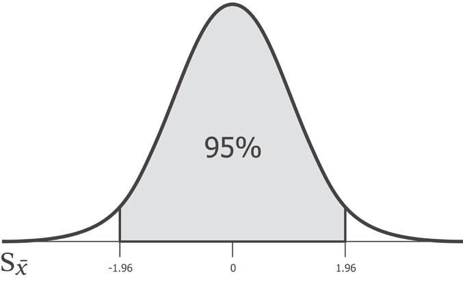
Какой бы ни была стандартная ошибка, 95% популяционного среднего значения будет находиться между -1.96 и 1.96 стандартных отклонений от выборочного среднего. И, следовательно, число 1.96 является критическим значением для 95%-ого интервала уверенности. Это критическое значение носит название z-значения.
Название z-значение вызвано тем, что нормальное распределение называется z-распределением. Впрочем, иногда z-значение так и называют — гауссовым значением.
Число 1.96 используется так широко, что его стоит запомнить. Впрочем, критическое значение мы можем вычислить сами, воспользовавшись функцией scipy stats.norm.ppf. Приведенная ниже функция confidence_interval ожидает значение для p между 0 и 1. Для нашего 95%-ого интервала уверенности оно будет равно 0.95. В целях вычисления положения каждого из двух хвостов нам нужно вычесть это число из единицы и разделить на 2 (2.5% для интервала уверенности шириной 95%):
def confidence_interval(p, xs):
    '''Интервал уверенности'''
    mu = xs.mean()
    se = standard_error(xs)
    z_crit = stats.norm.ppf(1 - (1-p) / 2)
    return [mu - z_crit * se, mu + z_crit * se]

def ex_2_9():
    '''Вычислить интервал уверенности
       для данных за определенный день'''
    may_1 = '2015-05-01'
    df    = with_parsed_date( load_data('dwell-times.tsv') )
    filtered = df.set_index( ['date'] )[may_1]
    ci = confidence_interval(0.95, filtered['dwell-time'])
    print('Интервал уверенности: ', ci)
Интервал уверенности: [83.53415272762004, 97.753065317492741]Полученный результат говорит о том, что можно на 95% быть уверенным в том, что популяционное среднее находится между 83.53 и 97.75 сек. И действительно, популяционное среднее, которое мы вычислили ранее, вполне укладывается в этот диапазон.
Сравнение выборок
После вирусной маркетинговой кампании веб-команда в AcmeContent извлекает для нас однодневную выборку времени пребывания посетителей на веб-сайте для проведения анализа. Они хотели бы узнать, не привлекла ли их недавняя кампания более активных посетителей веб-сайта. Интервалы уверенности предоставляют нам интуитивно понятный подход к сравнению двух выборок.
Точно так же, как мы делали ранее, мы загружаем значения времени пребывания, полученные в результате маркетинговой кампании, и их резюмируем:
def ex_2_10():
    '''Сводные статистики данных, полученных
       в результате вирусной кампании'''
    ts = load_data('campaign-sample.tsv')['dwell-time']
    print('n:                      ', ts.count())
    print('Среднее:                ', ts.mean())
    print('Медиана:                ', ts.median())
    print('Стандартное отклонение: ', ts.std())
    print('Стандартная ошибка:     ', standard_error(ts))

ex_2_10()
n: 300
Среднее: 130.22
Медиана: 84.0
Стандартное отклонение: 136.13370714388034
Стандартная ошибка: 7.846572839994115Среднее значение выглядит намного больше, чем то, которое мы видели ранее — 130 сек. по сравнению с 90 сек. Вполне возможно, здесь имеется некое значимое расхождение, хотя стандартная ошибка более чем в 2 раза больше той, которая была в предыдущей однодневной выборке, в силу меньшего размера выборки и большего стандартного отклонения. Основываясь на этих данных, можно вычислить 95%-й интервал уверенности для популяционного среднего, воспользовавшись для этого той же самой функцией confidence_interval, что и прежде:
def ex_2_11():
    '''Интервал уверенности для данных,
       полученных в результате вирусной кампании'''
    ts = load_data('campaign-sample.tsv')['dwell-time']
    print('Интервал уверенности:', confidence_interval(0.95, ts))
Интервал уверенности: [114.84099983154137, 145.59900016845864]95%-ый интервал уверенности для популяционного среднего лежит между 114.8 и 145.6 сек. Он вообще не пересекается с вычисленным нами ранее популяционным средним в размере 90 сек. Похоже, имеется какое-то крупное расхождение с опорной популяцией, которое едва бы произошло по причине одной лишь ошибки выборочного обследования. Наша задача теперь состоит в том, чтобы выяснить почему это происходит.
Ошибка выборочного обследования, также систематическая ошибка при взятии выборки, возникает, когда статистические характеристики популяции оцениваются исходя из подмножества этой популяции.
Искаженность
Выборка должна быть репрезентативной, то есть представлять популяцию, из которой она взята. Другими словами, при взятии выборки необходимо избегать искажения, которое происходит в результате того, что отдельно взятые члены популяции систематически из нее исключаются (либо в нее включаются) по сравнению с другими.
Широко известным примером искажения при взятии выборки является опрос населения, проведенный в США еженедельным журналом «Литературный Дайджест» (Literary Digest) по поводу президентских выборов 1936 г. Это был один из самых больших и самых дорогостоящих когда-либо проводившихся опросов: тогда по почте было опрошено 2.4 млн. человек. Результаты были однозначными — губернатор-республиканец от шт. Канзас Альфред Лэндон должен был победить Франклина Д. Рузвельта с 57% голосов. Как известно, в конечном счете на выборах победил Рузвельт с 62% голосов.
Первопричина допущенной журналом огромной ошибки выборочного обследования состояла в искажении при отборе. В своем стремлении собрать как можно больше адресов избирателей журнал «Литературный Дайджест» буквально выскреб все телефонные справочники, подписные перечни журнала и списки членов клубов. В эру, когда телефоны все еще во многом оставались предметом роскоши, такая процедура гарантировано имела избыточный вес в пользу избирателей, принадлежавших к верхнему и среднему классам, и не был представительным для электората в целом. Вторичной причиной искажения стала искаженность в результате неответов — в опросе фактически согласились участвовать всего менее четверти тех, к кому обратились. В этом виде искаженности при отборе предпочтение отдается только тем респондентам, которые действительно желают принять участие в голосовании.
Распространенный способ избежать искаженности при отборе состоит в том, чтобы каким-либо образом рандомизировать выборку. Введение в процедуру случайности делает вряд ли возможным, что экспериментальные факторы окажут неправомерное влияние на качество выборки. Опрос населения еженедельником «Литературный Дайджест» был сосредоточен на получении максимально возможной выборки, однако неискаженная малая выборка была бы намного полезнее, чем плохо отобранная большая выборка.
Если мы откроем файл campaign_sample.tsv, то обнаружим, что наша выборка приходится исключительно на 6 июня 2015 года. Это был выходной день, и этот факт мы можем легко подтвердить при помощи функции pandas:
'''Проверка даты'''
d = pd.to_datetime('2015 6 6')
d.weekday() in [5,6]TrueВсе наши сводные статистики до сих пор основывались на данных, которые мы отфильтровывали для получения только рабочих дней. Искаженность в нашей выборке вызвана именно этим фактом, и, если окажется, что поведение посетителей в выходные отличается от поведения в будние дни — вполне возможный сценарий — тогда мы скажем, что выборки представляют две разные популяции.
Визуализация разных популяций
Теперь снимем фильтр для рабочих дней и построим график среднесуточного времени пребывания для всех дней недели — рабочих и выходных:
def ex_2_12():
    '''Построить график времени ожидания
       по всем дням, без фильтра'''
    df = load_data('dwell-times.tsv')
    means = mean_dwell_times_by_date(df)['dwell-time']
    means.hist(bins=20)
    plt.xlabel('Ежедневное время ожидания неотфильтрованное, сек.')
    plt.ylabel('Частота')
    plt.show()
Этот пример сгенерирует следующую ниже гистограмму:

Распределение уже не является нормальным. Оно фактически является бимодальным, поскольку у него два пика. Второй меньший пик соответствует вновь добавленным выходным дням, и он ниже потому что количество выходных дней гораздо меньше количества рабочих дней, а также потому что стандартная ошибка распределения больше.
Распределения более чем с одним пиком обычно называются мультимодальными. Они могут указывать на совмещение двух или более нормальных распределений, и, следовательно, возможно, на совмещение двух или более популяций. Классическим примером бимодальности является распределение показателей роста людей, поскольку модальный рост мужчин выше, чем у женщин.
Данные выходных дней имеют другие характеристики в отличие от данных будних дней. Мы должны удостовериться, что мы сравниваем подобное с подобным. Отфильтруем наш первоначальный набор данных только по выходным дням:
def ex_2_13():
    '''Сводные статистики данных,
       отфильтрованных только по выходным дням'''
    df = with_parsed_date( load_data('dwell-times.tsv') )
    df.index = df['date']
    df = df[df['date'].index.dayofweek > 4]   # суббота-воскресенье
    weekend_times = df['dwell-time']

    print('n:                      ', weekend_times.count())
    print('Среднее:                ', weekend_times.mean())
    print('Медиана:                ', weekend_times.median())
    print('Стандартное отклонение: ', weekend_times.std())
    print('Стандартная ошибка:     ', standard_error(weekend_times))
n: 5860
Среднее: 117.78686006825939
Медиана: 81.0
Стандартное отклонение: 120.65234077179436
Стандартная ошибка: 1.5759770362547678Итоговое среднее значение в выходные дни (на основе 6-ти месячных данных) составляет 117.8 сек. и попадает в пределы 95%-ого интервала уверенности для маркетинговой выборки. Другими словами, хотя среднее значение времени пребывания в размере 130 сек. является высоким даже для выходных, расхождение не настолько большое, что его нельзя было бы приписать простой случайной изменчивости в выборке.
Мы только что применили подход к установлению подлинного расхождения в популяциях (между посетителями веб-сайта в выходные по сравнению с посетителями в будние дни), который при проведении проверки обычно не используется. Более традиционный подход начинается с выдвижения гипотетического предположения, после чего это предположение сверяется с данными. Для этих целей статистический метод анализа определяет строгий подход, который называется проверкой статистических гипотез.
Это и будет темой следующего поста, поста №3.
Примеры исходного кода для этого поста находятся в моем репо на Github. Все исходные данные взяты в репозитории автора книги.
A mathematical tool used in statistics to measure variability
What is Standard Error?
Standard error is a mathematical tool used in statistics to measure variability. It enables one to arrive at an estimation of what the standard deviation of a given sample is. It is commonly known by its abbreviated form – SE.

Standard error is used to estimate the efficiency, accuracy, and consistency of a sample. In other words, it measures how precisely a sampling distribution represents a population.
It can be applied in statistics and economics. It is especially useful in the field of econometrics, where researchers use it in performing regression analyses and hypothesis testing. It is also used in inferential statistics, where it forms the basis for the construction of the confidence intervals.
Some commonly used measures in the field of statistics include:
- Standard error of the mean (SEM)
- Standard error of the variance
- Standard error of the median
- Standard error of a regression coefficient
Calculating Standard Error of the Mean (SEM)
The SEM is calculated using the following formula:
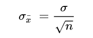
Where:
- σ – Population standard deviation
- n – Sample size, i.e., the number of observations in the sample
In a situation where statisticians are ignorant of the population standard deviation, they use the sample standard deviation as the closest replacement. SEM can then be calculated using the following formula. One of the primary assumptions here is that observations in the sample are statistically independent.
Where:
- s – Sample standard deviation
- n – Sample size, i.e., the number of observations in the sample
Importance of Standard Error
When a sample of observations is extracted from a population and the sample mean is calculated, it serves as an estimate of the population mean. Almost certainly, the sample mean will vary from the actual population mean. It will aid the statistician’s research to identify the extent of the variation. It is where the standard error of the mean comes into play.
When several random samples are extracted from a population, the standard error of the mean is essentially the standard deviation of different sample means from the population mean.
However, multiple samples may not always be available to the statistician. Fortunately, the standard error of the mean can be calculated from a single sample itself. It is calculated by dividing the standard deviation of the observations in the sample by the square root of the sample size.
Relationship between SEM and the Sample Size
Intuitively, as the sample size increases, the sample becomes more representative of the population.
For example, consider the marks of 50 students in a class in a mathematics test. Two samples A and B of 10 and 40 observations, respectively, are extracted from the population. It is logical to assert that the average marks in sample B will be closer to the average marks of the whole class than the average marks in sample A.
Thus, the standard error of the mean in sample B will be smaller than that in sample A. The standard error of the mean will approach zero with the increasing number of observations in the sample, as the sample becomes more and more representative of the population, and the sample mean approaches the actual population mean.
It is evident from the mathematical formula of the standard error of the mean that it is inversely proportional to the sample size. It can be verified using the SEM formula that if the sample size increases from 10 to 40 (becomes four times), the standard error will be half as big (reduces by a factor of 2).
Standard Deviation vs. Standard Error of the Mean
Standard deviation and standard error of the mean are both statistical measures of variability. While the standard deviation of a sample depicts the spread of observations within the given sample regardless of the population mean, the standard error of the mean measures the degree of dispersion of sample means around the population mean.
Related Readings
CFI is the official provider of the Business Intelligence & Data Analyst (BIDA)® certification program, designed to transform anyone into a world-class financial analyst.
To keep learning and developing your knowledge of financial analysis, we highly recommend the additional resources below:
- Coefficient of Variation
- Basic Statistics Concepts for Finance
- Regression Analysis
- Arithmetic Mean
- See all data science resources
In other sections of this guide on descriptive statistics, we taught you the basics of finding mean, median, standard deviation and percentiles. We provided you the formulas to each, as well as introduced some intermediate topics involving these measures of central tendency and variability. Here, we’ll present some advanced topics relating to these measures, namely the standard error and percentile rank.
Measures of Central Tendency and Variability
While measures like mean, median, standard deviation and percentiles can seem somewhat basic, the truth is that they are some of the most powerful tools of analysis within descriptive statistics and which form many of the fundamental concepts in more advanced, inferential statistics.
Percentiles, for example, is a concept that is used in quantile regression — which strives to identify patterns within different quantiles of a data set. These advanced applications rely on a strong, fundamental understanding of these more basic concepts. Below, you’ll find a brief recap of the formulas for sample mean, median and standard deviation as well as when they’re used and how to interpret them.
| Formula | Uses | Interpretation | |
| Mean |
|
|
The average of the data set, capturing where most values are cantered |
| Median | No standard formula, is found by identifying the middle value of ordered data |
|
The midpoint of the data, representing the point where half the data falls above and below |
| SD |
|
|
Is used to determine how typical a value is for a data set with a given mean and standard deviation |
![[ bar{x} = frac{Sigma x}{n} ]](https://www.superprof.co.uk/resources/wp-content/ql-cache/quicklatex.com-d2896fc12937c610d732a5a835db6ae0_l3.png "Rendered by QuickLaTeX.com")
![[ sqrt{ frac{Sigma (x_{i} - bar{x})^2 }{n-1} } ]](https://www.superprof.co.uk/resources/wp-content/ql-cache/quicklatex.com-06178b20f3e7e23c05f888333d2f97ee_l3.png "Rendered by QuickLaTeX.com")
![]()
The best tutors available
Let’s go
Standard Error
The concept of the standard deviation is a great starting point for understanding the standard error. It is defined as the estimate of the standard deviation of an estimate. Thus far, you’ve been calculating the standard deviation of an entire sample. Meaning, you’ve calculated a measure by which you can identify how likely any value would appear given the mean and sample size of your data set.
The standard deviation typically goes hand in hand with the distribution of a variable. Every distribution you will encounter reflects a probability density function, where each point on the horizontal axis corresponds with the probability of it occurring in a given data set on the vertical axis.
The question the standard deviation of a variable or data set attempts to answer is whether a given value is likely to be found for a given distribution. The question the standard error tries to answer is whether how likely a given statistic, such as the mean, is to be found for a given data set.
Instead of trying to find the distribution of a data set, the standard error tries to find the distribution of a given statistic. Recall the difference between a sample and a population. Measures of a population are called parameters, where the standard deviation of a parameter gives us information about the distribution of that parameter.
Measures of a sample, however, are estimates of parameters and are called statistics. The standard error, then, is an estimate of the standard deviation of a statistic.
If this is confusing, take the data sets below as an example. Each measure the test scores of students at different schools for the same test.
| Observation | School A | School B | School C |
| 1 | 45 | 29 | 66 |
| 2 | 64 | 54 | 57 |
| 3 | 38 | 59 | 58 |
| 4 | 70 | 67 | 52 |
| 5 | 62 | 68 | 32 |
| Mean | 56 | 55 | 53 |
Taking these three sample means, we can make an informed guess that the mean test score for the region is around 55 points. If we had information for ten more schools, then 100 more schools, and finally for all the schools in the region — we could start to get closer and closer to some middle value that may be higher or lower than 55 points.
Because we don’t always have the chance to take infinitely many samples, a probability distribution of means is a great way of estimating how likely a given mean is for a particular data set. In the table below, you’ll find the formulas for the standard deviation and the standard error of the mean for a population and sample, respectively.
| Population | Sample |
|
|
|
![[ sigma_{bar{x}} = frac{sigma}{sqrt{n}} ]](https://www.superprof.co.uk/resources/wp-content/ql-cache/quicklatex.com-f69388385c9e364e74f4d43ab862d7eb_l3.png "Rendered by QuickLaTeX.com")
![[ SE = frac{s}{sqrt{n}} ]](https://www.superprof.co.uk/resources/wp-content/ql-cache/quicklatex.com-bbfb08fc300d7cc36c4275845e664f98_l3.png "Rendered by QuickLaTeX.com")
Problem 1
Given the following dataset, what can you say about the accuracy of the average of the data?
| Observation | Value |
| 1 | 45 |
| 2 | 67 |
| 3 | 28 |
| 4 | 32 |
| 5 | 29 |
| 6 | 46 |
| 7 | 61 |
| 8 | 58 |
| 9 | 49 |
| 10 | 36 |
| 11 | 34 |
Problem 2
Given the following information, determine which data set has a lower standard error of mean.
| Observation | School A | School B | School C |
| Mean | 56 | 55 | 53 |
| SD | 4 | 10 | 8 |
| Sample Size | 9 | 1 000 | 250 |
Problem 3
Given the following chart, determine one of the measures of central tendency.

Problem 4
Given the following chart, choose which measure of central tendency would be most appropriate.

Solution Problem 1
In this problem, you were asked to:
- Say something about the accuracy of the mean
In this case, we first find the mean by following the steps below.
| Observation | Value |
| 1 | 45 |
| 2 | 67 |
| 3 | 28 |
| 4 | 32 |
| 5 | 29 |
| 6 | 46 |
| 7 | 61 |
| 8 | 58 |
| 9 | 49 |
| 10 | 36 |
| 11 | 34 |
| Total | 485 |
The mean is calculated as
![[ bar{x} = dfrac{485}{11} = 44.1 ]](https://www.superprof.co.uk/resources/wp-content/ql-cache/quicklatex.com-fc0538e0f7f6e734aa81b9a3fc677222_l3.png "Rendered by QuickLaTeX.com")
To find the accuracy of the mean, we need to calculate the standard error of the mean by first finding the standard deviation.
![[ s = sqrt{ dfrac{1832.91}{(11-1)} = 13.5 } ]](https://www.superprof.co.uk/resources/wp-content/ql-cache/quicklatex.com-d81102d0f8af1c5a35126a38b81796c2_l3.png "Rendered by QuickLaTeX.com")
Then, we plug the SD into the formula for standard error.
![[ SE = frac{s}{sqrt{n}} = dfrac{13.5}{sqrt{11}} = 4.1 ]](https://www.superprof.co.uk/resources/wp-content/ql-cache/quicklatex.com-780b872edbf0f0bd0ec8911404c0407f_l3.png "Rendered by QuickLaTeX.com")
Because the standard error is relatively small when compared to the dataset, this suggests the mean is pretty accurate.
Solution Problem 2
You were asked to determine which data set has a lower standard error of mean. Using the information given, you can calculate the standard error for each sample.
| Observation | School A | School B | School C |
| SE |
|
|
|
![[ = dfrac{4}{sqrt{9}} ]](https://www.superprof.co.uk/resources/wp-content/ql-cache/quicklatex.com-e445b3ec17512cd38ae7e8a362946f7e_l3.png "Rendered by QuickLaTeX.com")
![[ = 1.33 ]](https://www.superprof.co.uk/resources/wp-content/ql-cache/quicklatex.com-3eacc051ce66275344ec1eec046405c4_l3.png "Rendered by QuickLaTeX.com")
![[ =dfrac{10}{sqrt{1000}} ]](https://www.superprof.co.uk/resources/wp-content/ql-cache/quicklatex.com-f71d19b9c72d44e2b2e6227a386ff9b3_l3.png "Rendered by QuickLaTeX.com")
![[ = 0.32 ]](https://www.superprof.co.uk/resources/wp-content/ql-cache/quicklatex.com-84ed33b829fda45faba4b7d68f336485_l3.png "Rendered by QuickLaTeX.com")
![[ = dfrac{8}{sqrt{250}} ]](https://www.superprof.co.uk/resources/wp-content/ql-cache/quicklatex.com-74b53103167f7360399b15aef8106156_l3.png "Rendered by QuickLaTeX.com")
![[ = 0.51 ]](https://www.superprof.co.uk/resources/wp-content/ql-cache/quicklatex.com-f362cb11d3f150527cc00c20ad07f3e2_l3.png "Rendered by QuickLaTeX.com")
Based on the calculations performed in the table above, the sample with the lowest standard error of the mean is School B.
Solution Problem 3
The only measure of central tendency we can get from this chart is the mode, which is Chemistry.
Solution Problem 4
Because there are extreme values between 107 and 119, either the mode or the median would be most appropriate depending on what we’d like to investigate.
After reading this article you will learn about the standard of the mean.
Statistical inference also helps us to test the hypothesis that “the statistic based on the sample is not significantly different from the population parameter and that the difference if any noted is only due to chance variation”.
Standard Error of the mean (SEM or σM)
Standard Error of the mean (SEM) is quite important to test the representativeness or trustworthiness or significance of the mean.
Suppose that we have calculated the mean score of 200 boys of 10th grade of Delhi in the Numerical Ability Test to be 40. Thus 40 is the mean of only one sample drawn from the population (all the boys reading in class X in Delhi).
We can as well draw different random samples of 200 boys from the population. Suppose that we randomly choose 100 different samples, each sample consisting of 200 boys from the same population and compute the mean of each sample.
Although ‘n’ is 200 in each case, 200 boys chosen randomly to constitute the different samples are not identical and so due to fluctuation in sampling we would get 100 mean values from these 100 different samples.
These mean values will tend to differ from each other and they would form a series. These values form the sampling distribution of means. It can be expressed mathematically that these sample means are distributed normally.

The 100 mean values (in our example) will fall into a normal distribution around Mpop, the Mpop being the mean of the sampling distribution of means. The standard deviation of these 100 sample means is called SEM or Standard Error of the Mean which will be equal to the standard deviation of the population divided by square root of (sample size).
The SEM shows the spread of the sample means around Mpop. Thus SEM is a measure of variability of the sample means. It is a measure of divergence of sample means from Mpop. SEM is also written as σM.
Standard error of the mean (SEM or σM) is calculated by using the formula (for large samples)
(A) Calculation of SEM in Large Samples:
![]()
where σ = standard deviation of the population and
n = number of cases included in the sample
(As we can rarely have the S.D. of a population, for σ we use the value of S.D. of the sample means).
Confidence Interval:
The two confidence intervals i.e. 95% and 99% are in general use. R. A. Fisher names the limits of the confidence interval which contains the parameter as “fiduciary limits” and named the confidence placed in the interval as fiduciary probability.
(a) 95% of Confidence Interval:
Referring to the table of area under normal curve we find that 95% of cases lie between M± 1.96 SEM. That we are 95% confident or correct to say Mpop would lie in the interval M + 1.96 SEM and M + 1.96 SEM and we are 5% wrong to say that Mpop will lie out side this interval.
In other words probability of Mpop being in the range M± 1.96 SEM is 95% (or .95) and the probability of Mpop being outside the range is 5% (or .05). The value, 1.96 is the critical value at .05 level of significance.

(b) 99% of Confidence Interval:
Referring to the table of area under normal curve we find that 99% of cases lie between M±2.58 SEM. That we are 99% confident or correct to say Mpop would lie in the interval M – 2.58 SEM and M + 2.58 SEM and we are 1% wrong to say that Mpop will lie outside this interval.
In other words probability of Mpop being in the range M±2.58 SEM is 99% (or .99) and the probability of Mpop being outside the range is 1% (or .01). The value, 2.58 is the critical value at .01 level of significance.
Here we find that the level of significance is inversely related to the extent of precision. In 05 level of significance we would be accurate in 95% of cases and in .01 level of significance we would be accurate in 99% of eases.
The table stated below will precede you further:

Example 1:
The mean and S.D. of 225 boys of class XII of Delhi in a test of Numerical Ability were 48 and 6 respectively. How well this mean represent the Mpop or estimate Mpop. (n = 225, σ= 6, Mean = 48]
![]()
By referring to the table of normal distribution (Table A) we find that all most all (99.7) cases lie with in ± 3σ. In case of our example all the sample means will lie between Mpop + 3σm and Mpop – 3σM. So, any sample mean will be best 3σm less than Mpop on 3σM more than Mpop.
Thus if we know the value of σM we can infer about the Mpop from our sample mean. Here 4 is the standard deviation of the distribution of sample means of which our mean is one. All the sample means which are normally distributed around Mpop will lie between Mpop + 3 SEM and Mpop – 3 SEM.
3 SEM = 3 x .4 = 1.2
Although we do not know the exact value of Mpop we can at least say with confidence that Mpop lies in between
(48 -1.2) and (48 + 1.2) or 46.8 → 49.2
From Table A we find that 95% of eases lie between ± 1.96 σ. In case of our example 95% confidence interval for Mpop ranges from M – 1.96 SEM to M + 1.96 SEM.
Now, 1.96 SEM = 1.96 x .4 = .78
... M- 1.96 SEM = 48 – .78 = 47.22 and M + 1.96 SEM = 48 + .78 = 48.78
... 95% confidence interval ranges from 47.22 to 48.78. The 99% confidence interval for Mpop ranges from M – 2.58 SEM to M + 2.58 SEM.
Now 2.58 SEM = 2.58 X .4 = 1.03
... M – 2.58 SEM = 48 -1.03 = 46.97 and M + 2.58 SEM=48+ 1.03 =49.03
... 99% confidence interval for Mpop ranges from 46.97 to 49.03.
Example 2:
The mean and the S.D. of 400 students in a test were found to be 42 and 8. Can you estimate Mean score of the population at both 99% and 95% confidence interval?
Solution:

(i) 95% confidence interval for Mpop ranges from M – 1.96 SEM to M + 1.96 SEM.
Now 1.96 SEM = 1.96 x .4 = .784
... M-1.96 SEM = 42-.784 = 41.22
and M + 1.96 SEM = 42 + .784 = 42.78 (up to two decimals).
Thus 95% confidence interval ranges from 41.22 to 42.78. We are 95% accurate that Mpop lies between 41.22 to 42.78.
(ii) 99% confidence interval for Mpop ranges from M – 2.58 SEM to M + 2.58 SEM
Now 2.58 SEM = 2.58 x 4 = 1.03
... M – 2.58 SEM= 42- 1.03 =40.97
and M +2.58 SEM = 42 + 1.03 = 43.03
Thus 99% confidence interval ranges from 40.97 to 43.03. We are 99% confident that Mpop lies between 40.97 and 43.03.
Example 3:
The means and S.D. of a sample of 169 boys in a test of Numerical Ability are 50 and 6 respectively:
(i) Determine the 95% interval for the population mean and interpret it.
(ii) Determine the acceptable sampling error at .05 and .01 level of significance.
(iii) Determine 99% confidence interval for Mpop.
Solution:
![]()
M = 50
(i) 95% confidence interval for Mp0p ranges from M – 1.96 SEM to M + 1.96 SEM.
Now 1.96 SEm= 1.96 x .46 = .90
Thus M-1.96 SEM = 50-.90 = 49.10
and M+1.96 SEM = 50 +.90 = 50.90
... 95% confidence interval for Mpop ranges from 49.10 to 50.90. From the sample means of 50 we estimate the Mpop to be some fixed value in between 49.10 and 50.90 and in saying so we are 95% confident.
In other words, our sample mean of 50 will not miss the Mpop by more than .90 and this will be true for 95 cases in 100. Alternatively, only in 5 cases in 100 our sample mean of 50 will miss the Mpop by more than .90.
(ii) Critical value at .05 level of significance = 1.96
Critical value at .01 level of significance = 2.58
“Sampling error = Critical value x SEM”
Thus sampling error at .05 level of significance is 1.96 SEM and that at .01 level of significance is 2.58 SEM
Acceptable sampling error at .05 level = 1.96 SEM =1.96 x .46 = .90
Allowable sampling error at .01 level = 2.58 SEM = 2.58 X .46 = 1.19
(iii) The 99% confidence interval ranges from M – 2.58 SEM to M + 2.58 SEM
Now 2.58 SEM = 2.58 X .46 = 1.19
Thus M-2.58 SEM = 50- 1.19 = 48.81
and M +2.58 SEM = 50+1.19 = 51.19
99% confidence interval ranges from 48.81 to 51.19.
Example 4:
For a given group of 500 soldiers the mean AGCT score is 95.00 and SD is 25.
(ii) Determine the .99 confidence interval for the true mean.
(ii) It is unlikely that the true mean is larger than what value?
Solution:

(i) The 99% confidence interval ranges from M – 2.58 SEM to M + 2.58 SEM.
Now 2.58 SEM = 2.58 x 1.12 = 2.89
Thus M-2.58 SEM = 95.0-2.89 = 92.11
and M + 2.58 SEM = 95.0 + 2.89 = 97.89
... 99% confidence interval ranges from 92.11 to 97.89.
From our sample means of 95.0 we estimate the true mean to be some fixed value in between 92.11 and 97.89 and in say so we are 99% confident.
(ii) Our sample mean of 95.0 will not miss the true mean by more than 2.89 i.e., the true is not larger than 97.89.
(B) Calculation of SEM in small sample:
It is conventional to call any sample greater then 30 as large sample. When N is large, it is not worthwhile making the correction. But when N is “small” (less than 30), it is advisable to use (N – 1), and it is imperative when N is quite small- say, less than 10.
The student must remember (i) that theoretically (N – 1) should always be used when SD is to be an estimate of the population a ; and that (ii) the distinction between “large sample statistics” and “small sample statistics” in terms of a cutting point of N = 30 is arbitrary, and is in part a matter of convenience.
When N is less than about 30 the formula for the σM or SEM should read:


Example 5:
Following five students have secured scores in a test:
Determine the limits of 95% confidence limit for the population mean.
The scores are — 11, 13, 9, 12, 15:
Solution:

M=12

Here the df = n- 1=5-1=4
Refering Table D, with df= 4, the t-value at .05 level of significance (i.e. 95% confidence level) is 2.78.
The 95% confidence interval defines M ± 2.78 SEM
2.78 SEM=2.78 x 1.0 = 2.78
M – 2.78 SEM = 12 – 2.78 x1.0 = 9.22 and
M + 2.78 SEM = 12 + 2.78 x1.0= 14.78
.. . The limits of 95% confidence interval are 9.22 and 14.78.
This means that P = .95 that Mpop lies in the interval 9.22 to 14.78.
Example 6:
Ten measures of reaction time to light are taken from a practiced observer. The mean is 175.50 ms (milliseconds) and the S is 5.82 ms. Determine the .95 confidence interval for the Mpop; the .99 confidence interval.
Solution:
n = 10, S = 5.82 ms, M = 175.50 ms
![]()
The df(degrees of freedom) available for determining t are (n – 1) or (10 – 1) = 9
(i) Determining 95% (or. 95) confidence interval:
Entering Table D with 9 df, we read that t = 2.26 at the .05 point.
95% confidence interval for Mpop ranges from M – 2.26 SEM to M + 2.26 SEM.
Now 2.26 SEM = 2.26 x 1.84 = 4.16
Thus M – 2.26 SEM = 175.50 -4.16 = 171.34
and M + 2.26 SEM= 175.50 + 4.16 = 179.66
... 95% confidence interval for Mpop ranges from 171.34 to 179.66. The P is .95 that the Mpop is not less than 171.34 nor greater than 179.66. If we infer that Mpop lies within this interval, over a long series of experiments we should be right 95% of the time and wrong 5%.
(ii) Determining 99% (or .99) confidence interval:
Entering Table D with 9 df we read that t = 3.25 at .01 point. 99% confidence interval for Mpop ranges from M – 3.25 SEM to M + 3.25 SEM.
Now 3.25 SEM = 3.25 x 1.84 = 5.98
Thus M – 3.25 SEM = 175.50 – 5.98 = 169.52
and M + 3.25 SEM = 175.50 + 5.98 = 181.48
... 99% confidence interval for Mpop ranges from 169.52 to 181.48.
The P is .99 that the Mpop is not less than 169.52 nor greater than 181.48. If we infer that Mpop lies within this interval, over a long series of experiments we should be right -99% of the time and wrong 1%.
Inferences Regarding Other Statistics:
As all statistics have sampling distributions and standard errors the significance of the Median, Quartile Deviation, Standard Deviation, Percentages and other statistics can be interpreted like that of the mean and we can estimate the parameter.
(i) Standard Error of the Median (or SEMdn-):
In terms of SD and Q, the SE’s of the median for large samples can be calculated through following formulae:

in which σ = SD of the sample, n = size of the sample and Q = Quartile Deviation of the sample.
An example will illustrate the use and interpretation of the formulae:
Example 7:
On the Trabue Language Scale A, 801 eleven year-old boys made the following record:
Median = 21.40 and Q = 4.90. How well does this median represent the median of the population from which this sample is drawn?
Solution:
n = 801, Mdn = 21.40, Q = 4.90.
By applying the second formula, the
![]()
Since N is large, the sampling distribution may be taken to be normal and the confidence interval found from the last line in Table D. The .99 confidence interval for the Mdnpop is 21.40 ± 2.58 x .32 or 21.40 ± .83.
We may be confident that the median of the population is not less than 20.57 nor more than 22.23. This narrow range shows a high degree of trustworthiness in the sample median.
(ii) Standard Error of Standard Deviation (SEσ):
The standard error of standard deviation, like SEM, is found by computing the probable divergence of the sample SD from its parameter (population SD). The formula for SEσ is
![]()
Example 8:
n = 400, σ = 6
How well does this SD represent the SD of the population from which the sample is drawn?
Solution:
When samples are large and drawn at random from their population, above formula may be applied and interpreted in the same way as SEM.
![]()
Since N is large, the .99 confidence interval for SDpop can safely be taken at the limits ± 2.58 σσ. Substituting for σσ we have 6 ± 2.58 x .21 i.e. the limits between (6 – .54) and (6 + .54) or 5.46 and 6.54.
If we assume that the SDpop lies between the limits 5.46 and 6.54, we should be right 99% of the time and wrong 1%.
(iii) Standard Error of the Quartile Deviation (or SEQ or σq):
SEQ may be found from the formulae:
![]()
Example 9:
n = 801, Q = 4.90
How well does this Q represent the population Quartile Deviation?
Solution:
By applying the formula
![]()
The .99 confidence interval for the Qpop is from 4.90 ± 2.58 x .203 i.e. from 4.38 to 5.42. This range shows that the sample Q is a highly dependable statistics.
(iv) Standard Error of Percentage (or SE% or σ%):
Give the percentage occurrence of a behaviour, the question often arises of how much confidence we can place in the figure. How reliable an index is our percentage of the incidence of the behaviour in which we are interested? To answer this question,
We must compute the S.E. of a percentage by the formula:
![]()
in which
p = the percentage occurrence of the behaviour, q = (1 – p)
n = number of cases.
Example 10:
In a study of cheating among elementary-school children, 100 or 25% of the 400 children from homes of high socio-economic status were found to have cheated on various tests. How well does it represent the population percentage?
Solution:
![]()
p = 25% (percentage occurrence)
q = 75% (100% – 25%)
![]()
99% confidence interval for population percentage ranges from
25% ± 2.58 x 2.17%.
25% – 2.58 x 2.17% = 25% – 5.60% = 19.4%
and 25% + 2.58 x 2.17% = 25% + 5.60 = 30.60%
We can assume with 99% confidence that elementary school children of high socio-economic status would cheat with at least 19.4% and will not be larger than 30.60%.
(v) Standard Error of the Coefficient of Correlation (SEr or σr):
The classical formula for the S.E. of a- is
![]()
(SE of a coefficient of correlation r when N is large)
Example 11:
n = 120, r = .60.
What are the limits of 99% confidence interval for population r
Solution:
![]()
99% confidence interval
= r± 2.58 SEr = .60 ± 2.58 SEr
= .60 ± .15 or .45 to .75
Important Statistical Terms:
(i) Levels:
.05:
Probability of going wrong in 5 samples out of 100 samples.
.01:
Probability of going wrong in 1 sample out of 100 samples.
(ii) Confidence:
In .05 level of significance the experimenter has 95% confidence that the data must represent the population.
In .01 level of significance the experimenter has 99% confidence that sample statistic must represent the population.
(iii) Levels of Significance:
Before testing the hypothesis we have to decide the criteria with which we want to accept or reject the null hypothesis. We have to set up the level of significance prior to the test. Two levels of significance are in general use viz., .05 level and .01 level.
(a) .05 level of significance:
We read from Table A that 95% of the cases in a normal distribution fall within the limits ± 1.96 SEM. If we take the limits specified by M ± 1.96 SEM, we define an interval for which the level of confidence is .95. Basing our judgement as lo the size of Mpop on these limits, we stand to be right 95% of the time and wrong 5%.

The area between – 1.96 SEM and + 1.96 SEM is known as the area of acceptance of Ho and the area beyond – 1.96 SEM and + 1.96 SEM is known as the area of rejection. If any sample mean lies in the area of acceptance we accept the Ho. In rejecting the Ho we admit that the sample mean may fall outside ± 1.96 SEM.
Thus in rejecting Ho we make 5% error because in 5% out of 100 eases such a sample mean may occur. We are willing to take as much as 5% risk in rejecting Ho when it happens to be true. Thus the criteria for rejecting Ho is railed the level of significance.
(b) .01 level of significance:
We read from Table A that 99% of the eases in a normal distribution fall within the limits ± 2.58 SEM. If we lake the limits specified by M ± 2.58 SEM, we define an interval for which the level of confidence is .99. Basing our judgement as to the size of Mpop on these limits, we stand to be right 99% of the time and wrong 1%.
The area between – 2.58 SEM and + 2.58 SEM would be the area of acceptance of H0 and the area beyond it would be the area of rejection of Ho. We are willing to take as much as 1% risk in rejecting Ho when it happens to be true.
.01 level of significance is more exacting than the .05 level because in .01 level the error in rejecting Ho is 1% while in .05 level such error is 5%.

(iv) t-Distribution:
Whenever N is less than about 30 i.e., when the sample is small the sampling distribution is called “t-distribution”.
The t-distribution does not differ greatly from the normal unless N is quite small. As N increases in size the t distribution approaches more and more closely to the normal form.

Properties of t-distribution:
1. It looks like a bell-shaped curve. But its distribution is more variable with zero skewness and ‘Ku’ greater than 3.
2. It is symmetric about the line t = 0.
3. It is unimodal with maximum ordinate at t = 0.
4. When N is small, the t-distribution lies under the normal curve, but the tails or ends of the curve are higher than the corresponding parts of the normal curve.
5. The units along the baseline of the t-distribution are actually σ scores, i.e.,

(v) Degrees of Freedom (df):
The concept of degrees of freedom is highly important in small sample statistics. It is crucial too, in analysis of variance and in other procedures. Degrees of freedom means freedom to vary.
Let us choose five scores the mean of which is to be 15. Now suppose the four scores are 18, 10, 20, 15. For the mean to be equal to 15, the fifth score must be 12. We have, of course, freedom to choose any four scores.
But we have no freedom to choose the 5th score because the 5th score makes adjustments in the variation brought about by the first four scores and with an assumption that the mean will be 15. Here the N = 5 and one restriction is imposed i.e., the mean must be 15. Therefore, degree of freedom is N – 1 or 4.
If we have 5 scores 5, 6, 7, 8 and 9, the mean is 7; and the deviations of our scores from 7 are – 2, – 1, 0, 1 and 2. The sum of these deviations is zero. Of the 5 deviations, only 4 (N – 1) can be selected “freely” as the condition that the sum equal zero immediately restricts the value of the 5th deviate.
The SD is, of course, based upon the squares of the deviations taken around the mean. There are N df for computing the mean, but only (N – 1) available for the ‘S’ (the SD) as one df is lost in calculating the mean.
In another example, where N = 10, the df available for estimating the Mpop were given as 9 or (N – 1) i.e. one less than the number of observations, namely, 10. One df is lost in computing the M and accordingly only 9 are left for estimating the Mpop by way of ‘S’ and the t- distribution.
Whenever, a statistic is used to estimate a parameter, the rule is that the df available equals N minus the number of parameters already estimated from the sample. The M is an estimate of Mpop and in computing it we lose 1 df.
In estimating the dependability of an r, for example (which depends upon the deviations from two means), the df are (N – 2). In case of chi-square tests and analysis of variance separate procedures are followed in determining the df.
(vi) Null hypothesis:
The null hypothesis is a useful tool in testing the significance of differences. This hypothesis asserts that there is no true difference between two population means, and that the difference found between sample means is, therefore, accidental and unimportant.
The null hypothesis is related to the legal principle that “a man is innocent until he is proved guilty.” It constitutes a challenge and the function of an experiment is to give the facts a chance to refute (or fail to refute) this challenge.
To illustrate, suppose it is claimed that “instructional standards of single shift schools is better than the double shift schools”. This hypothesis is vaguely stated and cannot be tested precisely.
If we assert that “single shift schools do not yield better instructional standards than double shift schools” (the true difference being zero). This null hypothesis is exact and can be tested. If our null hypothesis is un-taxable, it must be rejected. The no-difference statement assumes that the two groups will be tested and found to be equal.
The null form is preferred by most of the experienced research personnel. This form of statement more readily defines the mathematical model to be utilized in the statistical test of hypothesis.
A null hypothesis is never proved or disproved. It may be accepted or rejected with certain degree of confidence (or at certain level of significance).
Before testing a hypothesis we must take into account of following:
1. Whether the sample is large or small.
2. What is the level of significance.
3. Whether the test is a two-tailed test or one-tailed test.
(vii) Errors in making inferences:
While accepting or rejecting null hypothesis there is possibility of committing two types of errors and lust be reckoned with by the research workers.
What are called Type I and Type II errors may be explained below:
Type I errors:
Such errors are Committed when we reject a null hypothesis by marking a difference significant, although there is no true difference. Suppose that the difference between two population means (Mpop – Mpop = 0) is actually zero. (For example, boys and girls may be thought of as constituting the same population with respect to most mental tests). If testing of significance of two sample means reflects a fact that the difference in population means is significant, we commit Type I error.
Type II errors:
Such type of errors are committed when we accept a null hypothesis by marking a difference not significant, although there is a true difference. Suppose there is a true difference between the two population means.
If our test of significance applied to the two sample means leads us to believe that the difference in population means is not significant we commit a Type II error.
Various precautions can be taken to avoid both sorts of errors. If we set up a low level of significance (P is greater than .05), we increase the likelihood of Type I errors; whereas, if we set up a high level of significance (P is less than .05), the Type I errors will be less. The possibility of drawing erroneous inferences of Type II sort is enhanced when we set a very high level of significance.
(viii) Two-tailed and One-tailed tests of significance:
In the null hypothesis differences between obtained means (i.e., M1 – M2) may be either plus or minus. In determining probabilities we take both tails of the sampling distribution.
(ix) Critical Ratio (CR):
Critical ratio (CR) is found by dividing the difference between the sample means by its standard error (CR = D/SED). When N’s of the samples are large (30 or more is “large”), the distribution of CR’s is known to be normal around the true difference between the population means, t is a critical ratio in which a more exact estimate of the σD is used. The sampling distribution of t is not normal when N is small (less than 30, say), t is a CR; but all CR’s are not t’s.
Two-tailed test:
1. In two-tailed test we take into consideration both the tails of the normal curve.
2. In case of non-tailed alternative hypothesis we make a two-tailed test.
3. Example:
An interest test is administered to certain boys in a vocational. Training class and to certain boys in a Latin class. Is the mean difference between the two groups significant at the .05 level?
4. The sample mean deviates from Mpop in either direction + or –.
5. H0: M1 – M2 = 0
HA: M1 = M2
6. Value to be significant:
1.96 at .05 level
2.58 at .01 level
7. The area of rejection is split at both the ends (tails) of normal curve (i.e. 05 into .025 and .025, 01 into .005 and .005).
One-tailed test:
1. We have to take one tall i.e. at the left hand or right side of normal curve into account.
2. In case of directional alternative hypothesis we make one-tailed test viz., M1 > M2. In such case direction is very much clear-one sided.
3. Example:
Ten subjects are given 5 successive trails upon a digit-symbol test of which only the scores for trails 1 and 5 are shown. Is the mean gain from initial to final trial significant?
4. The sample mean deviates from the population mean in one direction.
5. H0: M1 = M2
HA: M1 > M2 or M1 < m2
6. Value to be significant:
1.62 at .05 level
2.33 at .01 level
7. There is one rejection area at the right tail of the distribution or left tail of the distribution.

Estimate Standard Error of Median Using the Bootstrap Strategy
getting the Empirical Distribution through sampling with replacement
In this article, I will discuss the method we can use to estimate the standard error of the median. I will first specify some definitions and discuss how we can estimate the standard error of the mean. Then I will discuss how to estimate the standard error of the medium with the bootstrap strategy.
What is the standard error?
According to Wikipedia, the standard error of a statistic is the standard deviation of its sampling distribution or an estimate of that standard deviation. There are several concepts in this sentence that needs to be clarified before move forward:
First, a statistic is a sampling estimation of a parameter. For example, the sample mean x_bar is a statistic, while the population mean µ is a parameter. Since µ is usually unknown, we need a statistic to estimate it. x_bar is considered as an unbiased estimation of µ.
Second, the standard deviation is a measurement of dispersion, and it is the square root of variance. It usually stands for the confidence of your estimation and is used in the confidence interval, hypothesis testing, etc.
Last, a sampling distribution is the probability distribution of a statistic from random samples. Let’s take an example. Suppose we are estimating the average income of college graduates in the US. The population is the income of all graduates from college. It is almost impossible to collect the data from all graduates and estimate their incomes. That is why we are taking represented samples from the population and calculate the sample mean to estimate the population mean µ.
What is the standard error of the mean (SEM)?
Estimating the standard error of the mean is straightforward thanks to the Central Limit Theory. The theory stated that no matter what is the distribution of the population, the sampling distribution of the sample mean approaches a normal distribution as the sample size gets larger. In addition, the normal distribution has the mean equals to the population mean, and the standard deviation equals to population standard deviation divided by the square root of sample size n. Thus, the standard error of the mean is the sample standard deviation divided by the square root of sample size n, if the population standard deviation is unknown. Given any random distribution, we will estimate SEM easily.
How to estimate the standard error of the median?
Unfortunately, the Central Limit Theory does not apply to the median, thus we need other methods to estimate the standard error of the median given only one sample. That is when the bootstrap strategy comes in handy.
The bootstrap is sampling with replacement. If there is a sample:

we can take n items from this sample with replacement. Here, we will generate a new sample, it can be:

with a sample size equals to n. Using the bootstrap strategy to estimate standard error follows the steps as stated below:
1, take n items from the given sample as a new sample:
from this sample, we can easily calculate the sample median:
2, repeat the previous procedure for B rounds, and we will get B new samples, with B sample medians:
3, now we have got an empirical distribution of medians, thus we can estimate the standard error of medians from them:
(1) calculate the mean of the previous sample of medians:

(2) calculate the variation:
(2) calculate the standard error, which is the standard deviation of the empirical sample:
Why is bootstrap working?
The reason bootstrap works is that bootstrap uses the Empirical Distribution Function (EDF) to estimate the CDF of the population. A statistic of a sample is a function of a sample randomly taken from the population. Thus its distribution will depend on the CDF of the population and the sample size. While the CDF of a population is usually unknown, we can estimate it using EDF, thus get the sample statistic distribution from it. We can find here the detailed mathematical explanation, along with some other restrictions.
Hope this helps! Thank you for reading!
![]()
How to estimate the standard error of the median: The Bootstrap Strategy was originally published in Towards Data Science on Medium, where people are continuing the conversation by highlighting and responding to this story.