Метод рунге кутта ошибка

Методы Рунге-Кутта.

Методы
Рунге-Кутта решения дифференциальных
уравнений, как и метод Эйлера, принадлежат
к классу одношаговых методов. Они
являются своеобразным обобщением этого
класса и обладают рядом достоинств:

обладают
достаточно высокой точностью;
допускают
использование переменного шага, что
даёт возможность уменьшить его там,
где значения функции быстро изменяются,
и увеличить его в противном случае;
являются
легко применимыми, так как для начала
расчёта достаточно выбрать сетку х_n
и задать значение y₀=f(x₀).

Наиболее часто
применяют метод Рунге-Кутта четвертого
порядка

Рассмотрим
разложение функции (решения ДУ) в
окрестности произвольной точки x_n

где
h_n=x_n₊₁-x_n.

Ограничимся в
разложении функции 3 первыми слагаемыми
ряда, т.е.

.
(*)

Тогда остаточный
член в виде формы Тейлора представится
в виде

или
погрешность, при условии, что 3 производная
ограничена на (х_n;
x_n₊₁),
имеет порядок О(h³).

Вторую
производную в формуле (*) можно найти
непосредственно из ДУ

y=f(x,y),

как
производную от функции, заданной неявно.
Получим

Подставив данное
выражение в(*), получим

Однако
такой подход не всегда приемлем, т.к.
связан с отысканием частных производных
функции. Чтобы избежать этого вторую
производную можно представить в виде

где
,,
– некоторые параметры.

Тогда
.

Преобразуем данное
выражение

(**).

Заменим приращение
функции 2 переменных её дифференциалом

на

В
нашем случае

Тогда
.

и
общая формула примет вид

После
преобразований получим

Обозначим
.

Получим

Сравнивая
коэффициенты при степенях h
точного решения (по формуле Тейлора) и
приближённого, получим систему уравнений
для определения параметров ,
,
J,


Для
определения 4 неизвестных имеем систему
3 уравнений. Такая система имеет
бесчисленное множество решений. Выразим
через 
все остальные параметры. Получим

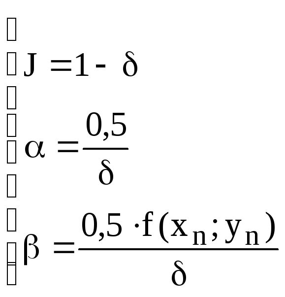Подставляя в (**)
эти параметры, получим

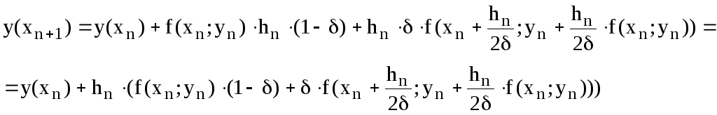
Таким
образом мы получили однопараметрическое
семейство схем Рунге Кутта 4 порядка
точности.

Не
трудно заметить, что подставляя вместо
,
получается формула усовершенствованного
метода Эйлера.

Однако
в таком виде метод Рунге- Кутта в связи
с неопределённостью коэффициента 
использовать не будем.

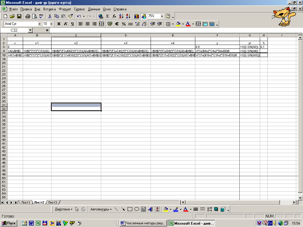
Приведем
расчетные формулы метода для решения
задач:

y_i₊₁=y_i+(K₁+2K₂+2K₃+K₄)/6

(4.12)

Для
оценки значения производной в этом
методе используется четыре вспомогательных
шага на которых предварительно вычисляются
величины

К₁=hf(x_i,y_i);

;

К₄=
hf(x_i+h,y_i+K₃);

i
= 1, 2, 3,….. .

(4.13)

В
данном методе ошибка на шаге вычислений
имеет порядок h⁴.

Поскольку
большинство систем ДУ и ДУ высших
порядков могут быть сведены ДУ первого
порядка рассмотренные методы можно
применять для их решения.

Погрешность схем Рунге –Кутта. Правило Рунге.

Одним
из наиболее простых, широко применяемых
и достаточно эффективных методов оценки
погрешности и уточнения полученных
результатов в приближённых вычислениях
с использованием сеток является правило
Рунге.

Пусть
имеется приближённая формула
для вычисления величиныy(x)
по значениям на равномерной сетке h_n
и остаточный член этой формулы имеет
вид:

Выполним
теперь расчёт по той же приближённой
формуле для той же точки х, но используя
равномерную сетку с другим шагом rh
r<1.
Тогда полученное значение
связано с точным значением соотношением

Заметим,
что =

Тогда
имея два расчёта на разных сетках,
нетрудно оценить величину погрешности

Первое
из слагаемых есть главный член погрешности.
Таким образом, расчёт по второй сетке
позволяет оценить погрешность расчёта
по первой с точностью до членов более
высокого порядка. При этом достаточная
точность будет достигнута, если величина
R
не превышает заданной погрешности во
всех совпадающих узлах. Чаще всего в
качестве шагов приближённого вычисления
решения уравнения выбирают h
и h/2.
Грубо шаг вычислений можно оценить
исходя из неравенства
.

Соседние файлы в предмете [НЕСОРТИРОВАННОЕ]

Источник

In numerical analysis, the Runge–Kutta methods ( RUUNG-ə-KUUT-tah^[1]) are a family of implicit and explicit iterative methods, which include the Euler method, used in temporal discretization for the approximate solutions of simultaneous nonlinear equations.^[2] These methods were developed around 1900 by the German mathematicians Carl Runge and Wilhelm Kutta.

Comparison of the Runge-Kutta methods for the differential equation ${displaystyle y'=sin(t)^{2}cdot y}$ (red is the exact solution)

The Runge–Kutta method[edit]

Slopes used by the classical Runge-Kutta method

The most widely known member of the Runge–Kutta family is generally referred to as «RK4», the «classic Runge–Kutta method» or simply as «the Runge–Kutta method».

Let an initial value problem be specified as follows:

${displaystyle {frac {dy}{dt}}=f(t,y),quad y(t_{0})=y_{0}.}$

Here is an unknown function (scalar or vector) of time , which we would like to approximate; we are told that ${frac {dy}{dt}}$ , the rate at which changes, is a function of and of itself. At the initial time $t_{0}$ the corresponding value is $y_{0}$ . The function and the initial conditions $t_{0}$ , $y_{0}$ are given.

Now we pick a step-size h > 0 and define:

${displaystyle {begin{aligned}y_{n+1}&=y_{n}+{frac {1}{6}}left(k_{1}+2k_{2}+2k_{3}+k_{4}right)h,\t_{n+1}&=t_{n}+h\end{aligned}}}$

for n = 0, 1, 2, 3, …, using^[3]

${displaystyle {begin{aligned}k_{1}&= f(t_{n},y_{n}),\k_{2}&= f!left(t_{n}+{frac {h}{2}},y_{n}+h{frac {k_{1}}{2}}right),\k_{3}&= f!left(t_{n}+{frac {h}{2}},y_{n}+h{frac {k_{2}}{2}}right),\k_{4}&= f!left(t_{n}+h,y_{n}+hk_{3}right).end{aligned}}}$

(Note: the above equations have different but equivalent definitions in different texts).^[4]

Here $y_{n+1}$ is the RK4 approximation of $y(t_{n+1})$ , and the next value ( $y_{n+1}$ ) is determined by the present value ( $y_{n}$ ) plus the weighted average of four increments, where each increment is the product of the size of the interval, h, and an estimated slope specified by function f on the right-hand side of the differential equation.

In averaging the four slopes, greater weight is given to the slopes at the midpoint. If is independent of , so that the differential equation is equivalent to a simple integral, then RK4 is Simpson’s rule.^[5]

The RK4 method is a fourth-order method, meaning that the local truncation error is on the order of $O(h^{5})$ , while the total accumulated error is on the order of $O(h^{4})$ .

In many practical applications the function is independent of (so called autonomous system, or time-invariant system, especially in physics), and their increments are not computed at all and not passed to function , with only the final formula for $t_{n+1}$ used.

Explicit Runge–Kutta methods[edit]

The family of explicit Runge–Kutta methods is a generalization of the RK4 method mentioned above. It is given by

$y_{n+1}=y_{n}+hsum _{i=1}^{s}b_{i}k_{i},$

where^[6]

${displaystyle {begin{aligned}k_{1}&=f(t_{n},y_{n}),\k_{2}&=f(t_{n}+c_{2}h,y_{n}+(a_{21}k_{1})h),\k_{3}&=f(t_{n}+c_{3}h,y_{n}+(a_{31}k_{1}+a_{32}k_{2})h),\& vdots \k_{s}&=f(t_{n}+c_{s}h,y_{n}+(a_{s1}k_{1}+a_{s2}k_{2}+cdots +a_{s,s-1}k_{s-1})h).end{aligned}}}$

(Note: the above equations may have different but equivalent definitions in some texts).^[4]

To specify a particular method, one needs to provide the integer s (the number of stages), and the coefficients a_ij (for 1 ≤ j < i ≤ s), b_i (for i = 1, 2, …, s) and c_i (for i = 2, 3, …, s). The matrix [a_ij] is called the Runge–Kutta matrix, while the b_i and c_i are known as the weights and the nodes.^[7] These data are usually arranged in a mnemonic device, known as a Butcher tableau (after John C. Butcher):


$c_{2}$	$a_{21}$
$c_{3}$	$a_{31}$	$a_{32}$

$c_{s}$	$a_{s1}$	$a_{s2}$	$a_{s,s-1}$
	$b_{1}$	$b_{2}$	$b_{s-1}$	$b_{s}$

A Taylor series expansion shows that the Runge–Kutta method is consistent if and only if

${displaystyle sum _{i=1}^{s}b_{i}=1.}$

There are also accompanying requirements if one requires the method to have a certain order p, meaning that the local truncation error is O(h^p⁺¹). These can be derived from the definition of the truncation error itself. For example, a two-stage method has order 2 if b₁ + b₂ = 1, b₂c₂ = 1/2, and b₂a₂₁ = 1/2.^[8] Note that a popular condition for determining coefficients is ^[9]

${displaystyle sum _{j=1}^{i-1}a_{ij}=c_{i}{text{ for }}i=2,ldots ,s.}$

This condition alone, however, is neither sufficient, nor necessary for consistency.
^[10]

In general, if an explicit -stage Runge–Kutta method has order , then it can be proven that the number of stages must satisfy sgeq p , and if pgeq 5 , then .^[11]
However, it is not known whether these bounds are sharp in all cases; for example, all known methods of order 8 have at least 11 stages, though it is possible that there are methods with fewer stages. (The bound above suggests that there could be a method with 9 stages; but it could also be that the bound is simply not sharp.) Indeed, it is an open problem
what the precise minimum number of stages is for an explicit Runge–Kutta method to have order in those cases where no methods have yet been discovered that satisfy the bounds above with equality. Some values which are known are:^[12]

${begin{array}{c|cccccccc}p&1&2&3&4&5&6&7&8\hline min s&1&2&3&4&6&7&9&11end{array}}$

The provable bounds above then imply that we can not find methods of orders that require fewer stages than the methods we already know for these orders. However, it is conceivable that we might find a method of order p=7 that has only 8 stages, whereas the only ones known today have at least 9 stages as shown in the table.

Examples[edit]

The RK4 method falls in this framework. Its tableau is^[13]

0
1/2	1/2
1/2	0	1/2
1	0	0	1
	1/6	1/3	1/3	1/6

A slight variation of «the» Runge–Kutta method is also due to Kutta in 1901 and is called the 3/8-rule.^[14] The primary advantage this method has is that almost all of the error coefficients are smaller than in the popular method, but it requires slightly more FLOPs (floating-point operations) per time step. Its Butcher tableau is

0
1/3	1/3
2/3	-1/3	1
1	1	−1	1
	1/8	3/8	3/8	1/8

However, the simplest Runge–Kutta method is the (forward) Euler method, given by the formula ${displaystyle y_{n+1}=y_{n}+hf(t_{n},y_{n})}$ . This is the only consistent explicit Runge–Kutta method with one stage. The corresponding tableau is

Second-order methods with two stages[edit]

An example of a second-order method with two stages is provided by the midpoint method:

${displaystyle y_{n+1}=y_{n}+hfleft(t_{n}+{frac {1}{2}}h,y_{n}+{frac {1}{2}}hf(t_{n}, y_{n})right).}$

The corresponding tableau is

The midpoint method is not the only second-order Runge–Kutta method with two stages; there is a family of such methods, parameterized by α and given by the formula^[15]

$y_{n+1}=y_{n}+h{bigl (}(1-{tfrac {1}{2alpha }})f(t_{n},y_{n})+{tfrac {1}{2alpha }}f(t_{n}+alpha h,y_{n}+alpha hf(t_{n},y_{n})){bigr )}.$

Its Butcher tableau is

In this family, $alpha ={tfrac {1}{2}}$ gives the midpoint method, is Heun’s method,^[5] and ${displaystyle alpha ={tfrac {2}{3}}}$ is Ralston’s method.

Use[edit]

As an example, consider the two-stage second-order Runge–Kutta method with α = 2/3, also known as Ralston method. It is given by the tableau

0
2/3	2/3
	1/4	3/4

with the corresponding equations

${displaystyle {begin{aligned}k_{1}&=f(t_{n}, y_{n}),\k_{2}&=f(t_{n}+{tfrac {2}{3}}h, y_{n}+{tfrac {2}{3}}hk_{1}),\y_{n+1}&=y_{n}+hleft({tfrac {1}{4}}k_{1}+{tfrac {3}{4}}k_{2}right).end{aligned}}}$

This method is used to solve the initial-value problem

${displaystyle {frac {dy}{dt}}=tan(y)+1,quad y_{0}=1, tin [1,1.1]}$

with step size h = 0.025, so the method needs to take four steps.

The method proceeds as follows:

$t_{0}=1colon$
	$y_{0}=1$
$t_{1}=1.025colon$
	$y_{0}=1$	$k_{1}=2.557407725$	${displaystyle k_{2}=f(t_{0}+{tfrac {2}{3}}h, y_{0}+{tfrac {2}{3}}hk_{1})=2.7138981400}$
	$y_{1}=y_{0}+h({tfrac {1}{4}}k_{1}+{tfrac {3}{4}}k_{2})={underline {1.066869388}}$
$t_{2}=1.05colon$
	$y_{1}=1.066869388$	$k_{1}=2.813524695$	${displaystyle k_{2}=f(t_{1}+{tfrac {2}{3}}h, y_{1}+{tfrac {2}{3}}hk_{1})}$
	$y_{2}=y_{1}+h({tfrac {1}{4}}k_{1}+{tfrac {3}{4}}k_{2})={underline {1.141332181}}$
$t_{3}=1.075colon$
	$y_{2}=1.141332181$	$k_{1}=3.183536647$	${displaystyle k_{2}=f(t_{2}+{tfrac {2}{3}}h, y_{2}+{tfrac {2}{3}}hk_{1})}$
	$y_{3}=y_{2}+h({tfrac {1}{4}}k_{1}+{tfrac {3}{4}}k_{2})={underline {1.227417567}}$
$t_{4}=1.1colon$
	$y_{3}=1.227417567$	$k_{1}=3.796866512$	${displaystyle k_{2}=f(t_{3}+{tfrac {2}{3}}h, y_{3}+{tfrac {2}{3}}hk_{1})}$
	$y_{4}=y_{3}+h({tfrac {1}{4}}k_{1}+{tfrac {3}{4}}k_{2})={underline {1.335079087}}.$

The numerical solutions correspond to the underlined values.

Adaptive Runge–Kutta methods[edit]

Adaptive methods are designed to produce an estimate of the local truncation error of a single Runge–Kutta step. This is done by having two methods, one with order and one with order p-1 . These methods are interwoven, i.e., they have common intermediate steps. Thanks to this, estimating the error has little or negligible computational cost compared to a step with the higher-order method.

During the integration, the step size is adapted such that the estimated error stays below a user-defined threshold: If the error is too high, a step is repeated with a lower step size; if the error is much smaller, the step size is increased to save time. This results in an (almost) optimal step size, which saves computation time. Moreover, the user does not have to spend time on finding an appropriate step size.

The lower-order step is given by

$y_{n+1}^{*}=y_{n}+hsum _{i=1}^{s}b_{i}^{*}k_{i},$

where $k_{i}$ are the same as for the higher-order method. Then the error is

$e_{n+1}=y_{n+1}-y_{n+1}^{*}=hsum _{i=1}^{s}(b_{i}-b_{i}^{*})k_{i},$

which is $O(h^{p})$ .
The Butcher tableau for this kind of method is extended to give the values of $b_{i}^{*}$ :

0
$c_{2}$	$a_{21}$
$c_{3}$	$a_{31}$	$a_{32}$

$c_{s}$	$a_{s1}$	$a_{s2}$	$a_{s,s-1}$
	$b_{1}$	$b_{2}$	$b_{s-1}$	$b_{s}$
	$b_{1}^{*}$	$b_{2}^{*}$	$b_{s-1}^{*}$	$b_{s}^{*}$

The Runge–Kutta–Fehlberg method has two methods of orders 5 and 4. Its extended Butcher tableau is:

0
1/4	1/4
3/8	3/32	9/32
12/13	1932/2197	−7200/2197	7296/2197
1	439/216	−8	3680/513	-845/4104
1/2	−8/27	2	−3544/2565	1859/4104	−11/40
	16/135	0	6656/12825	28561/56430	−9/50	2/55
	25/216	0	1408/2565	2197/4104	−1/5	0

However, the simplest adaptive Runge–Kutta method involves combining Heun’s method, which is order 2, with the Euler method, which is order 1. Its extended Butcher tableau is:

0
1	1
	1/2	1/2
	1	0

Other adaptive Runge–Kutta methods are the Bogacki–Shampine method (orders 3 and 2), the Cash–Karp method and the Dormand–Prince method (both with orders 5 and 4).

Nonconfluent Runge–Kutta methods[edit]

A Runge–Kutta method is said to be nonconfluent ^[16] if all the $c_{i},,i=1,2,ldots ,s$ are distinct.

Runge–Kutta–Nyström methods[edit]

Runge–Kutta–Nyström methods are specialized Runge-Kutta methods that are optimized for second-order differential equations of the following form:^[17]^[18]

${displaystyle {frac {d^{2}y}{dt^{2}}}=f(y,{dot {y}},t).}$

Implicit Runge–Kutta methods[edit]

All Runge–Kutta methods mentioned up to now are explicit methods. Explicit Runge–Kutta methods are generally unsuitable for the solution of stiff equations because their region of absolute stability is small; in particular, it is bounded.^[19]
This issue is especially important in the solution of partial differential equations.

The instability of explicit Runge–Kutta methods motivates the development of implicit methods. An implicit Runge–Kutta method has the form

$y_{n+1}=y_{n}+hsum _{i=1}^{s}b_{i}k_{i},$

where

${displaystyle k_{i}=fleft(t_{n}+c_{i}h, y_{n}+hsum _{j=1}^{s}a_{ij}k_{j}right),quad i=1,ldots ,s.}$

^[20]

The difference with an explicit method is that in an explicit method, the sum over j only goes up to i − 1. This also shows up in the Butcher tableau: the coefficient matrix $a_{ij}$ of an explicit method is lower triangular. In an implicit method, the sum over j goes up to s and the coefficient matrix is not triangular, yielding a Butcher tableau of the form^[13]

${displaystyle {begin{array}{c|cccc}c_{1}&a_{11}&a_{12}&dots &a_{1s}\c_{2}&a_{21}&a_{22}&dots &a_{2s}\vdots &vdots &vdots &ddots &vdots \c_{s}&a_{s1}&a_{s2}&dots &a_{ss}\hline &b_{1}&b_{2}&dots &b_{s}\&b_{1}^{*}&b_{2}^{*}&dots &b_{s}^{*}\end{array}}={begin{array}{c|c}mathbf {c} &A\hline &mathbf {b^{T}} \end{array}}}$

See Adaptive Runge-Kutta methods above for the explanation of the b^* row.

The consequence of this difference is that at every step, a system of algebraic equations has to be solved. This increases the computational cost considerably. If a method with s stages is used to solve a differential equation with m components, then the system of algebraic equations has ms components. This can be contrasted with implicit linear multistep methods (the other big family of methods for ODEs): an implicit s-step linear multistep method needs to solve a system of algebraic equations with only m components, so the size of the system does not increase as the number of steps increases.^[21]

Examples[edit]

The simplest example of an implicit Runge–Kutta method is the backward Euler method:

${displaystyle y_{n+1}=y_{n}+hf(t_{n}+h, y_{n+1}).,}$

The Butcher tableau for this is simply:

${begin{array}{c|c}1&1\hline &1\end{array}}$

This Butcher tableau corresponds to the formulae

${displaystyle k_{1}=f(t_{n}+h, y_{n}+hk_{1})quad {text{and}}quad y_{n+1}=y_{n}+hk_{1},}$

which can be re-arranged to get the formula for the backward Euler method listed above.

Another example for an implicit Runge–Kutta method is the trapezoidal rule. Its Butcher tableau is:

${displaystyle {begin{array}{c|cc}0&0&0\1&{frac {1}{2}}&{frac {1}{2}}\hline &{frac {1}{2}}&{frac {1}{2}}\&1&0\end{array}}}$

The trapezoidal rule is a collocation method (as discussed in that article). All collocation methods are implicit Runge–Kutta methods, but not all implicit Runge–Kutta methods are collocation methods.^[22]

The Gauss–Legendre methods form a family of collocation methods based on Gauss quadrature. A Gauss–Legendre method with s stages has order 2s (thus, methods with arbitrarily high order can be constructed).^[23] The method with two stages (and thus order four) has Butcher tableau:

${displaystyle {begin{array}{c|cc}{frac {1}{2}}-{frac {1}{6}}{sqrt {3}}&{frac {1}{4}}&{frac {1}{4}}-{frac {1}{6}}{sqrt {3}}\{frac {1}{2}}+{frac {1}{6}}{sqrt {3}}&{frac {1}{4}}+{frac {1}{6}}{sqrt {3}}&{frac {1}{4}}\hline &{frac {1}{2}}&{frac {1}{2}}\&{frac {1}{2}}+{frac {1}{2}}{sqrt {3}}&{frac {1}{2}}-{frac {1}{2}}{sqrt {3}}end{array}}}$

^[21]

Stability[edit]

The advantage of implicit Runge–Kutta methods over explicit ones is their greater stability, especially when applied to stiff equations. Consider the linear test equation . A Runge–Kutta method applied to this equation reduces to the iteration $y_{n+1}=r(hlambda ),y_{n}$ , with r given by

$r(z)=1+zb^{T}(I-zA)^{-1}e={frac {det(I-zA+zeb^{T})}{det(I-zA)}},$

^[24]

where e stands for the vector of ones. The function r is called the stability function.^[25] It follows from the formula that r is the quotient of two polynomials of degree s if the method has s stages. Explicit methods have a strictly lower triangular matrix A, which implies that det(I − zA) = 1 and that the stability function is a polynomial.^[26]

The numerical solution to the linear test equation decays to zero if | r(z) | < 1 with z = hλ. The set of such z is called the domain of absolute stability. In particular, the method is said to be absolute stable if all z with Re(z) < 0 are in the domain of absolute stability. The stability function of an explicit Runge–Kutta method is a polynomial, so explicit Runge–Kutta methods can never be A-stable.^[26]

If the method has order p, then the stability function satisfies $r(z)={textrm {e}}^{z}+O(z^{p+1})$ as zto 0 . Thus, it is of interest to study quotients of polynomials of given degrees that approximate the exponential function the best. These are known as Padé approximants. A Padé approximant with numerator of degree m and denominator of degree n is A-stable if and only if m ≤ n ≤ m + 2.^[27]

The Gauss–Legendre method with s stages has order 2s, so its stability function is the Padé approximant with m = n = s. It follows that the method is A-stable.^[28] This shows that A-stable Runge–Kutta can have arbitrarily high order. In contrast, the order of A-stable linear multistep methods cannot exceed two.^[29]

B-stability[edit]

The A-stability concept for the solution of differential equations is related to the linear autonomous equation . Dahlquist proposed the investigation of stability of numerical schemes when applied to nonlinear systems that satisfy a monotonicity condition. The corresponding concepts were defined as G-stability for multistep methods (and the related one-leg methods) and B-stability (Butcher, 1975) for Runge–Kutta methods. A Runge–Kutta method applied to the non-linear system y'=f(y) , which verifies , is called B-stable, if this condition implies $|y_{n+1}-z_{n+1}|leq |y_{n}-z_{n}|$ for two numerical solutions.

Let , and be three matrices defined by

${displaystyle B=operatorname {diag} (b_{1},b_{2},ldots ,b_{s}),,M=BA+A^{T}B-bb^{T},,Q=BA^{-1}+A^{-T}B-A^{-T}bb^{T}A^{-1}.}$

A Runge–Kutta method is said to be algebraically stable^[30] if the matrices and are both non-negative definite. A sufficient condition for B-stability^[31] is: and are non-negative definite.

Derivation of the Runge–Kutta fourth-order method[edit]

In general a Runge–Kutta method of order can be written as:

$y_{t+h}=y_{t}+hcdot sum _{i=1}^{s}a_{i}k_{i}+{mathcal {O}}(h^{s+1}),$

where:

${displaystyle k_{i}=y_{t}+hcdot sum _{j=1}^{s}beta _{ij}fleft(k_{j}, t_{n}+alpha _{i}hright)}$

are increments obtained evaluating the derivatives of $y_{t}$ at the -th order.

We develop the derivation^[32] for the Runge–Kutta fourth-order method using the general formula with s=4 evaluated, as explained above, at the starting point, the midpoint and the end point of any interval ; thus, we choose:

${displaystyle {begin{aligned}&alpha _{i}&&beta _{ij}\alpha _{1}&=0&beta _{21}&={frac {1}{2}}\alpha _{2}&={frac {1}{2}}&beta _{32}&={frac {1}{2}}\alpha _{3}&={frac {1}{2}}&beta _{43}&=1\alpha _{4}&=1&&\end{aligned}}}$

and $beta _{ij}=0$ otherwise. We begin by defining the following quantities:

${displaystyle {begin{aligned}y_{t+h}^{1}&=y_{t}+hfleft(y_{t}, tright)\y_{t+h}^{2}&=y_{t}+hfleft(y_{t+h/2}^{1}, t+{frac {h}{2}}right)\y_{t+h}^{3}&=y_{t}+hfleft(y_{t+h/2}^{2}, t+{frac {h}{2}}right)end{aligned}}}$

where $y_{t+h/2}^{1}={dfrac {y_{t}+y_{t+h}^{1}}{2}}$ and $y_{t+h/2}^{2}={dfrac {y_{t}+y_{t+h}^{2}}{2}}$ .
If we define:

${displaystyle {begin{aligned}k_{1}&=f(y_{t}, t)\k_{2}&=fleft(y_{t+h/2}^{1}, t+{frac {h}{2}}right)=fleft(y_{t}+{frac {h}{2}}k_{1}, t+{frac {h}{2}}right)\k_{3}&=fleft(y_{t+h/2}^{2}, t+{frac {h}{2}}right)=fleft(y_{t}+{frac {h}{2}}k_{2}, t+{frac {h}{2}}right)\k_{4}&=fleft(y_{t+h}^{3}, t+hright)=fleft(y_{t}+hk_{3}, t+hright)end{aligned}}}$

and for the previous relations we can show that the following equalities hold up to ${mathcal {O}}(h^{2})$ :

${displaystyle {begin{aligned}k_{2}&=fleft(y_{t+h/2}^{1}, t+{frac {h}{2}}right)=fleft(y_{t}+{frac {h}{2}}k_{1}, t+{frac {h}{2}}right)\&=fleft(y_{t}, tright)+{frac {h}{2}}{frac {d}{dt}}fleft(y_{t}, tright)\k_{3}&=fleft(y_{t+h/2}^{2}, t+{frac {h}{2}}right)=fleft(y_{t}+{frac {h}{2}}fleft(y_{t}+{frac {h}{2}}k_{1}, t+{frac {h}{2}}right), t+{frac {h}{2}}right)\&=fleft(y_{t}, tright)+{frac {h}{2}}{frac {d}{dt}}left[fleft(y_{t}, tright)+{frac {h}{2}}{frac {d}{dt}}fleft(y_{t}, tright)right]\k_{4}&=fleft(y_{t+h}^{3}, t+hright)=fleft(y_{t}+hfleft(y_{t}+{frac {h}{2}}k_{2}, t+{frac {h}{2}}right), t+hright)\&=fleft(y_{t}+hfleft(y_{t}+{frac {h}{2}}fleft(y_{t}+{frac {h}{2}}fleft(y_{t}, tright), t+{frac {h}{2}}right), t+{frac {h}{2}}right), t+hright)\&=fleft(y_{t}, tright)+h{frac {d}{dt}}left[fleft(y_{t}, tright)+{frac {h}{2}}{frac {d}{dt}}left[fleft(y_{t}, tright)+{frac {h}{2}}{frac {d}{dt}}fleft(y_{t}, tright)right]right]end{aligned}}}$

where:

${displaystyle {frac {d}{dt}}f(y_{t}, t)={frac {partial }{partial y}}f(y_{t}, t){dot {y}}_{t}+{frac {partial }{partial t}}f(y_{t}, t)=f_{y}(y_{t}, t){dot {y}}+f_{t}(y_{t}, t):={ddot {y}}_{t}}$

is the total derivative of with respect to time.

If we now express the general formula using what we just derived we obtain:

${displaystyle {begin{aligned}y_{t+h}={}&y_{t}+hleftlbrace acdot f(y_{t}, t)+bcdot left[f(y_{t}, t)+{frac {h}{2}}{frac {d}{dt}}f(y_{t}, t)right]right.+\&{}+ccdot left[f(y_{t}, t)+{frac {h}{2}}{frac {d}{dt}}left[fleft(y_{t}, tright)+{frac {h}{2}}{frac {d}{dt}}f(y_{t}, t)right]right]+\&{}+dcdot left[f(y_{t}, t)+h{frac {d}{dt}}left[f(y_{t}, t)+{frac {h}{2}}{frac {d}{dt}}left[f(y_{t}, t)+left.{frac {h}{2}}{frac {d}{dt}}f(y_{t}, t)right]right]right]rightrbrace +{mathcal {O}}(h^{5})\={}&y_{t}+acdot hf_{t}+bcdot hf_{t}+bcdot {frac {h^{2}}{2}}{frac {df_{t}}{dt}}+ccdot hf_{t}+ccdot {frac {h^{2}}{2}}{frac {df_{t}}{dt}}+\&{}+ccdot {frac {h^{3}}{4}}{frac {d^{2}f_{t}}{dt^{2}}}+dcdot hf_{t}+dcdot h^{2}{frac {df_{t}}{dt}}+dcdot {frac {h^{3}}{2}}{frac {d^{2}f_{t}}{dt^{2}}}+dcdot {frac {h^{4}}{4}}{frac {d^{3}f_{t}}{dt^{3}}}+{mathcal {O}}(h^{5})end{aligned}}}$

and comparing this with the Taylor series of $y_{t+h}$ around :

${displaystyle {begin{aligned}y_{t+h}&=y_{t}+h{dot {y}}_{t}+{frac {h^{2}}{2}}{ddot {y}}_{t}+{frac {h^{3}}{6}}y_{t}^{(3)}+{frac {h^{4}}{24}}y_{t}^{(4)}+{mathcal {O}}(h^{5})=\&=y_{t}+hf(y_{t}, t)+{frac {h^{2}}{2}}{frac {d}{dt}}f(y_{t}, t)+{frac {h^{3}}{6}}{frac {d^{2}}{dt^{2}}}f(y_{t}, t)+{frac {h^{4}}{24}}{frac {d^{3}}{dt^{3}}}f(y_{t}, t)end{aligned}}}$

we obtain a system of constraints on the coefficients:

${displaystyle {begin{cases}&a+b+c+d=1\[6pt]&{frac {1}{2}}b+{frac {1}{2}}c+d={frac {1}{2}}\[6pt]&{frac {1}{4}}c+{frac {1}{2}}d={frac {1}{6}}\[6pt]&{frac {1}{4}}d={frac {1}{24}}end{cases}}}$

which when solved gives $a={frac {1}{6}},b={frac {1}{3}},c={frac {1}{3}},d={frac {1}{6}}$ as stated above.

Notes[edit]

^ «Runge-Kutta method». Dictionary.com. Retrieved 4 April 2021.
^ DEVRIES, Paul L. ; HASBUN, Javier E. A first course in computational physics. Second edition. Jones and Bartlett Publishers: 2011. p. 215.
^ Press et al. 2007, p. 908; Süli & Mayers 2003, p. 328
^ ^a ^b Atkinson (1989, p. 423), Hairer, Nørsett & Wanner (1993, p. 134), Kaw & Kalu (2008, §8.4) and Stoer & Bulirsch (2002, p. 476) leave out the factor h in the definition of the stages. Ascher & Petzold (1998, p. 81), Butcher (2008, p. 93) and Iserles (1996, p. 38) use the y values as stages.
^ ^a ^b Süli & Mayers 2003, p. 328
^ Press et al. 2007, p. 907
^ Iserles 1996, p. 38
^ Iserles 1996, p. 39
^ Iserles 1996, p. 39
^
As a counterexample, consider any explicit 2-stage Runge-Kutta scheme with ${displaystyle b_{1}=b_{2}=1/2}$ and $c_{1}$ and $a_{21}$ randomly chosen. This method is consistent and (in general) first-order convergent. On the other hand, the 1-stage method with ${displaystyle b_{1}=1/2}$ is inconsistent and fails to converge, even though it trivially holds that ${displaystyle sum _{j=1}^{i-1}a_{ij}=c_{i}{text{ for }}i=2,ldots ,s.}$ .
^ Butcher 2008, p. 187
^ Butcher 2008, pp. 187–196
^ ^a ^b Süli & Mayers 2003, p. 352
^ Hairer, Nørsett & Wanner (1993, p. 138) refer to Kutta (1901).
^ Süli & Mayers 2003, p. 327
^ Lambert 1991, p. 278
^ Dormand, J. R.; Prince, P. J. (October 1978). «New Runge–Kutta Algorithms for Numerical Simulation in Dynamical Astronomy». Celestial Mechanics. 18 (3): 223–232. Bibcode:1978CeMec..18..223D. doi:10.1007/BF01230162. S2CID 120974351.
^ Fehlberg, E. (October 1974). Classical seventh-, sixth-, and fifth-order Runge–Kutta–Nyström formulas with stepsize control for general second-order differential equations (Report) (NASA TR R-432 ed.). Marshall Space Flight Center, AL: National Aeronautics and Space Administration.
^ Süli & Mayers 2003, pp. 349–351
^ Iserles 1996, p. 41; Süli & Mayers 2003, pp. 351–352
^ ^a ^b Süli & Mayers 2003, p. 353
^ Iserles 1996, pp. 43–44
^ Iserles 1996, p. 47
^ Hairer & Wanner 1996, pp. 40–41
^ Hairer & Wanner 1996, p. 40
^ ^a ^b Iserles 1996, p. 60
^ Iserles 1996, pp. 62–63
^ Iserles 1996, p. 63
^ This result is due to Dahlquist (1963).
^ Lambert 1991, p. 275
^ Lambert 1991, p. 274
^ Lyu, Ling-Hsiao (August 2016). «Appendix C. Derivation of the Numerical Integration Formulae» (PDF). Numerical Simulation of Space Plasmas (I) Lecture Notes. Institute of Space Science, National Central University. Retrieved 17 April 2022.

References[edit]

Runge, Carl David Tolmé (1895), «Über die numerische Auflösung von Differentialgleichungen», Mathematische Annalen, Springer, 46 (2): 167–178, doi:10.1007/BF01446807, S2CID 119924854.
Kutta, Wilhelm (1901), «Beitrag zur näherungsweisen Integration totaler Differentialgleichungen», Zeitschrift für Mathematik und Physik, 46: 435–453.
Ascher, Uri M.; Petzold, Linda R. (1998), Computer Methods for Ordinary Differential Equations and Differential-Algebraic Equations, Philadelphia: Society for Industrial and Applied Mathematics, ISBN 978-0-89871-412-8.
Atkinson, Kendall A. (1989), An Introduction to Numerical Analysis (2nd ed.), New York: John Wiley & Sons, ISBN 978-0-471-50023-0.
Butcher, John C. (May 1963), «Coefficients for the study of Runge-Kutta integration processes», Journal of the Australian Mathematical Society, 3 (2): 185–201, doi:10.1017/S1446788700027932.
Butcher, John C. (May 1964), «On Runge-Kutta processes of high order», Journal of the Australian Mathematical Society, 4 (2): 179–194, doi:10.1017/S1446788700023387
Butcher, John C. (1975), «A stability property of implicit Runge-Kutta methods», BIT, 15 (4): 358–361, doi:10.1007/bf01931672, S2CID 120854166.
Butcher, John C. (2000), «Numerical methods for ordinary differential equations in the 20th century», J. Comp. Appl. Math., 125 (1–2): 1–29, doi:10.1016/S0377-0427(00)00455-6.
Butcher, John C. (2008), Numerical Methods for Ordinary Differential Equations, New York: John Wiley & Sons, ISBN 978-0-470-72335-7.
Cellier, F.; Kofman, E. (2006), Continuous System Simulation, Springer Verlag, ISBN 0-387-26102-8.
Dahlquist, Germund (1963), «A special stability problem for linear multistep methods», BIT, 3: 27–43, doi:10.1007/BF01963532, hdl:10338.dmlcz/103497, ISSN 0006-3835, S2CID 120241743.
Forsythe, George E.; Malcolm, Michael A.; Moler, Cleve B. (1977), Computer Methods for Mathematical Computations, Prentice-Hall (see Chapter 6).
Hairer, Ernst; Nørsett, Syvert Paul; Wanner, Gerhard (1993), Solving ordinary differential equations I: Nonstiff problems, Berlin, New York: Springer-Verlag, ISBN 978-3-540-56670-0.
Hairer, Ernst; Wanner, Gerhard (1996), Solving ordinary differential equations II: Stiff and differential-algebraic problems (2nd ed.), Berlin, New York: Springer-Verlag, ISBN 978-3-540-60452-5.
Iserles, Arieh (1996), A First Course in the Numerical Analysis of Differential Equations, Cambridge University Press, ISBN 978-0-521-55655-2.
Lambert, J.D (1991), Numerical Methods for Ordinary Differential Systems. The Initial Value Problem, John Wiley & Sons, ISBN 0-471-92990-5
Kaw, Autar; Kalu, Egwu (2008), Numerical Methods with Applications (1st ed.), autarkaw.com.
Press, William H.; Teukolsky, Saul A.; Vetterling, William T.; Flannery, Brian P. (2007), «Section 17.1 Runge-Kutta Method», Numerical Recipes: The Art of Scientific Computing (3rd ed.), Cambridge University Press, ISBN 978-0-521-88068-8. Also, Section 17.2. Adaptive Stepsize Control for Runge-Kutta.
Stoer, Josef; Bulirsch, Roland (2002), Introduction to Numerical Analysis (3rd ed.), Berlin, New York: Springer-Verlag, ISBN 978-0-387-95452-3.
Süli, Endre; Mayers, David (2003), An Introduction to Numerical Analysis, Cambridge University Press, ISBN 0-521-00794-1.
Tan, Delin; Chen, Zheng (2012), «On A General Formula of Fourth Order Runge-Kutta Method» (PDF), Journal of Mathematical Science & Mathematics Education, 7 (2): 1–10.
advance discrete maths ignou reference book (code- mcs033)
John C. Butcher: «B-Series : Algebraic Analysis of Numerical Methods», Springer（SSCM, volume 55), ISBN 978-3030709556 (April, 2021).

External links[edit]

«Runge-Kutta method», Encyclopedia of Mathematics, EMS Press, 2001 [1994]
Runge–Kutta 4th-Order Method
Tracker Component Library Implementation in Matlab — Implements 32 embedded Runge Kutta algorithms in RungeKStep, 24 embedded Runge-Kutta Nyström algorithms in RungeKNystroemSStep and 4 general Runge-Kutta Nyström algorithms in RungeKNystroemGStep.

Источник

Comparison of the Runge-Kutta methods for the differential equation ${displaystyle y'=sin(t)^{2}cdot y}$ (red is the exact solution)

The Runge–Kutta method[edit]

Slopes used by the classical Runge-Kutta method

The most widely known member of the Runge–Kutta family is generally referred to as «RK4», the «classic Runge–Kutta method» or simply as «the Runge–Kutta method».

Let an initial value problem be specified as follows:

${displaystyle {frac {dy}{dt}}=f(t,y),quad y(t_{0})=y_{0}.}$

Now we pick a step-size h > 0 and define:

${displaystyle {begin{aligned}y_{n+1}&=y_{n}+{frac {1}{6}}left(k_{1}+2k_{2}+2k_{3}+k_{4}right)h,\t_{n+1}&=t_{n}+h\end{aligned}}}$

for n = 0, 1, 2, 3, …, using^[3]

(Note: the above equations have different but equivalent definitions in different texts).^[4]

The RK4 method is a fourth-order method, meaning that the local truncation error is on the order of $O(h^{5})$ , while the total accumulated error is on the order of $O(h^{4})$ .

Explicit Runge–Kutta methods[edit]

The family of explicit Runge–Kutta methods is a generalization of the RK4 method mentioned above. It is given by

$y_{n+1}=y_{n}+hsum _{i=1}^{s}b_{i}k_{i},$

where^[6]

(Note: the above equations may have different but equivalent definitions in some texts).^[4]


$c_{2}$	$a_{21}$
$c_{3}$	$a_{31}$	$a_{32}$

$c_{s}$	$a_{s1}$	$a_{s2}$	$a_{s,s-1}$
	$b_{1}$	$b_{2}$	$b_{s-1}$	$b_{s}$

A Taylor series expansion shows that the Runge–Kutta method is consistent if and only if

${displaystyle sum _{i=1}^{s}b_{i}=1.}$

${displaystyle sum _{j=1}^{i-1}a_{ij}=c_{i}{text{ for }}i=2,ldots ,s.}$

This condition alone, however, is neither sufficient, nor necessary for consistency.
^[10]

${begin{array}{c|cccccccc}p&1&2&3&4&5&6&7&8\hline min s&1&2&3&4&6&7&9&11end{array}}$

Examples[edit]

The RK4 method falls in this framework. Its tableau is^[13]

0
1/2	1/2
1/2	0	1/2
1	0	0	1
	1/6	1/3	1/3	1/6

0
1/3	1/3
2/3	-1/3	1
1	1	−1	1
	1/8	3/8	3/8	1/8

Second-order methods with two stages[edit]

An example of a second-order method with two stages is provided by the midpoint method:

${displaystyle y_{n+1}=y_{n}+hfleft(t_{n}+{frac {1}{2}}h,y_{n}+{frac {1}{2}}hf(t_{n}, y_{n})right).}$

The corresponding tableau is

The midpoint method is not the only second-order Runge–Kutta method with two stages; there is a family of such methods, parameterized by α and given by the formula^[15]

$y_{n+1}=y_{n}+h{bigl (}(1-{tfrac {1}{2alpha }})f(t_{n},y_{n})+{tfrac {1}{2alpha }}f(t_{n}+alpha h,y_{n}+alpha hf(t_{n},y_{n})){bigr )}.$

Its Butcher tableau is

In this family, $alpha ={tfrac {1}{2}}$ gives the midpoint method, is Heun’s method,^[5] and ${displaystyle alpha ={tfrac {2}{3}}}$ is Ralston’s method.

Use[edit]

As an example, consider the two-stage second-order Runge–Kutta method with α = 2/3, also known as Ralston method. It is given by the tableau

0
2/3	2/3
	1/4	3/4

with the corresponding equations

${displaystyle {begin{aligned}k_{1}&=f(t_{n}, y_{n}),\k_{2}&=f(t_{n}+{tfrac {2}{3}}h, y_{n}+{tfrac {2}{3}}hk_{1}),\y_{n+1}&=y_{n}+hleft({tfrac {1}{4}}k_{1}+{tfrac {3}{4}}k_{2}right).end{aligned}}}$

This method is used to solve the initial-value problem

${displaystyle {frac {dy}{dt}}=tan(y)+1,quad y_{0}=1, tin [1,1.1]}$

with step size h = 0.025, so the method needs to take four steps.

The method proceeds as follows:

$t_{0}=1colon$
	$y_{0}=1$
$t_{1}=1.025colon$
	$y_{0}=1$	$k_{1}=2.557407725$	${displaystyle k_{2}=f(t_{0}+{tfrac {2}{3}}h, y_{0}+{tfrac {2}{3}}hk_{1})=2.7138981400}$
	$y_{1}=y_{0}+h({tfrac {1}{4}}k_{1}+{tfrac {3}{4}}k_{2})={underline {1.066869388}}$
$t_{2}=1.05colon$
	$y_{1}=1.066869388$	$k_{1}=2.813524695$	${displaystyle k_{2}=f(t_{1}+{tfrac {2}{3}}h, y_{1}+{tfrac {2}{3}}hk_{1})}$
	$y_{2}=y_{1}+h({tfrac {1}{4}}k_{1}+{tfrac {3}{4}}k_{2})={underline {1.141332181}}$
$t_{3}=1.075colon$
	$y_{2}=1.141332181$	$k_{1}=3.183536647$	${displaystyle k_{2}=f(t_{2}+{tfrac {2}{3}}h, y_{2}+{tfrac {2}{3}}hk_{1})}$
	$y_{3}=y_{2}+h({tfrac {1}{4}}k_{1}+{tfrac {3}{4}}k_{2})={underline {1.227417567}}$
$t_{4}=1.1colon$
	$y_{3}=1.227417567$	$k_{1}=3.796866512$	${displaystyle k_{2}=f(t_{3}+{tfrac {2}{3}}h, y_{3}+{tfrac {2}{3}}hk_{1})}$
	$y_{4}=y_{3}+h({tfrac {1}{4}}k_{1}+{tfrac {3}{4}}k_{2})={underline {1.335079087}}.$

The numerical solutions correspond to the underlined values.

Adaptive Runge–Kutta methods[edit]

The lower-order step is given by

$y_{n+1}^{*}=y_{n}+hsum _{i=1}^{s}b_{i}^{*}k_{i},$

where $k_{i}$ are the same as for the higher-order method. Then the error is

$e_{n+1}=y_{n+1}-y_{n+1}^{*}=hsum _{i=1}^{s}(b_{i}-b_{i}^{*})k_{i},$

which is $O(h^{p})$ .
The Butcher tableau for this kind of method is extended to give the values of $b_{i}^{*}$ :

0
$c_{2}$	$a_{21}$
$c_{3}$	$a_{31}$	$a_{32}$

$c_{s}$	$a_{s1}$	$a_{s2}$	$a_{s,s-1}$
	$b_{1}$	$b_{2}$	$b_{s-1}$	$b_{s}$
	$b_{1}^{*}$	$b_{2}^{*}$	$b_{s-1}^{*}$	$b_{s}^{*}$

The Runge–Kutta–Fehlberg method has two methods of orders 5 and 4. Its extended Butcher tableau is:

0
1/4	1/4
3/8	3/32	9/32
12/13	1932/2197	−7200/2197	7296/2197
1	439/216	−8	3680/513	-845/4104
1/2	−8/27	2	−3544/2565	1859/4104	−11/40
	16/135	0	6656/12825	28561/56430	−9/50	2/55
	25/216	0	1408/2565	2197/4104	−1/5	0

However, the simplest adaptive Runge–Kutta method involves combining Heun’s method, which is order 2, with the Euler method, which is order 1. Its extended Butcher tableau is:

0
1	1
	1/2	1/2
	1	0

Other adaptive Runge–Kutta methods are the Bogacki–Shampine method (orders 3 and 2), the Cash–Karp method and the Dormand–Prince method (both with orders 5 and 4).

Nonconfluent Runge–Kutta methods[edit]

A Runge–Kutta method is said to be nonconfluent ^[16] if all the $c_{i},,i=1,2,ldots ,s$ are distinct.

Runge–Kutta–Nyström methods[edit]

Runge–Kutta–Nyström methods are specialized Runge-Kutta methods that are optimized for second-order differential equations of the following form:^[17]^[18]

${displaystyle {frac {d^{2}y}{dt^{2}}}=f(y,{dot {y}},t).}$

Implicit Runge–Kutta methods[edit]

The instability of explicit Runge–Kutta methods motivates the development of implicit methods. An implicit Runge–Kutta method has the form

$y_{n+1}=y_{n}+hsum _{i=1}^{s}b_{i}k_{i},$

where

${displaystyle k_{i}=fleft(t_{n}+c_{i}h, y_{n}+hsum _{j=1}^{s}a_{ij}k_{j}right),quad i=1,ldots ,s.}$

^[20]

See Adaptive Runge-Kutta methods above for the explanation of the b^* row.

Examples[edit]

The simplest example of an implicit Runge–Kutta method is the backward Euler method:

${displaystyle y_{n+1}=y_{n}+hf(t_{n}+h, y_{n+1}).,}$

The Butcher tableau for this is simply:

${begin{array}{c|c}1&1\hline &1\end{array}}$

This Butcher tableau corresponds to the formulae

${displaystyle k_{1}=f(t_{n}+h, y_{n}+hk_{1})quad {text{and}}quad y_{n+1}=y_{n}+hk_{1},}$

which can be re-arranged to get the formula for the backward Euler method listed above.

Another example for an implicit Runge–Kutta method is the trapezoidal rule. Its Butcher tableau is:

${displaystyle {begin{array}{c|cc}0&0&0\1&{frac {1}{2}}&{frac {1}{2}}\hline &{frac {1}{2}}&{frac {1}{2}}\&1&0\end{array}}}$

^[21]

Stability[edit]

$r(z)=1+zb^{T}(I-zA)^{-1}e={frac {det(I-zA+zeb^{T})}{det(I-zA)}},$

^[24]

B-stability[edit]

Let , and be three matrices defined by

${displaystyle B=operatorname {diag} (b_{1},b_{2},ldots ,b_{s}),,M=BA+A^{T}B-bb^{T},,Q=BA^{-1}+A^{-T}B-A^{-T}bb^{T}A^{-1}.}$

A Runge–Kutta method is said to be algebraically stable^[30] if the matrices and are both non-negative definite. A sufficient condition for B-stability^[31] is: and are non-negative definite.

Derivation of the Runge–Kutta fourth-order method[edit]

In general a Runge–Kutta method of order can be written as:

$y_{t+h}=y_{t}+hcdot sum _{i=1}^{s}a_{i}k_{i}+{mathcal {O}}(h^{s+1}),$

where:

${displaystyle k_{i}=y_{t}+hcdot sum _{j=1}^{s}beta _{ij}fleft(k_{j}, t_{n}+alpha _{i}hright)}$

are increments obtained evaluating the derivatives of $y_{t}$ at the -th order.

and $beta _{ij}=0$ otherwise. We begin by defining the following quantities:

where $y_{t+h/2}^{1}={dfrac {y_{t}+y_{t+h}^{1}}{2}}$ and $y_{t+h/2}^{2}={dfrac {y_{t}+y_{t+h}^{2}}{2}}$ .
If we define:

and for the previous relations we can show that the following equalities hold up to ${mathcal {O}}(h^{2})$ :

where:

${displaystyle {frac {d}{dt}}f(y_{t}, t)={frac {partial }{partial y}}f(y_{t}, t){dot {y}}_{t}+{frac {partial }{partial t}}f(y_{t}, t)=f_{y}(y_{t}, t){dot {y}}+f_{t}(y_{t}, t):={ddot {y}}_{t}}$

is the total derivative of with respect to time.

If we now express the general formula using what we just derived we obtain:

and comparing this with the Taylor series of $y_{t+h}$ around :

we obtain a system of constraints on the coefficients:

${displaystyle {begin{cases}&a+b+c+d=1\[6pt]&{frac {1}{2}}b+{frac {1}{2}}c+d={frac {1}{2}}\[6pt]&{frac {1}{4}}c+{frac {1}{2}}d={frac {1}{6}}\[6pt]&{frac {1}{4}}d={frac {1}{24}}end{cases}}}$

which when solved gives $a={frac {1}{6}},b={frac {1}{3}},c={frac {1}{3}},d={frac {1}{6}}$ as stated above.

Notes[edit]

^ «Runge-Kutta method». Dictionary.com. Retrieved 4 April 2021.
^ DEVRIES, Paul L. ; HASBUN, Javier E. A first course in computational physics. Second edition. Jones and Bartlett Publishers: 2011. p. 215.
^ Press et al. 2007, p. 908; Süli & Mayers 2003, p. 328
^ ^a ^b Atkinson (1989, p. 423), Hairer, Nørsett & Wanner (1993, p. 134), Kaw & Kalu (2008, §8.4) and Stoer & Bulirsch (2002, p. 476) leave out the factor h in the definition of the stages. Ascher & Petzold (1998, p. 81), Butcher (2008, p. 93) and Iserles (1996, p. 38) use the y values as stages.
^ ^a ^b Süli & Mayers 2003, p. 328
^ Press et al. 2007, p. 907
^ Iserles 1996, p. 38
^ Iserles 1996, p. 39
^ Iserles 1996, p. 39
^
As a counterexample, consider any explicit 2-stage Runge-Kutta scheme with ${displaystyle b_{1}=b_{2}=1/2}$ and $c_{1}$ and $a_{21}$ randomly chosen. This method is consistent and (in general) first-order convergent. On the other hand, the 1-stage method with ${displaystyle b_{1}=1/2}$ is inconsistent and fails to converge, even though it trivially holds that ${displaystyle sum _{j=1}^{i-1}a_{ij}=c_{i}{text{ for }}i=2,ldots ,s.}$ .
^ Butcher 2008, p. 187
^ Butcher 2008, pp. 187–196
^ ^a ^b Süli & Mayers 2003, p. 352
^ Hairer, Nørsett & Wanner (1993, p. 138) refer to Kutta (1901).
^ Süli & Mayers 2003, p. 327
^ Lambert 1991, p. 278
^ Dormand, J. R.; Prince, P. J. (October 1978). «New Runge–Kutta Algorithms for Numerical Simulation in Dynamical Astronomy». Celestial Mechanics. 18 (3): 223–232. Bibcode:1978CeMec..18..223D. doi:10.1007/BF01230162. S2CID 120974351.
^ Fehlberg, E. (October 1974). Classical seventh-, sixth-, and fifth-order Runge–Kutta–Nyström formulas with stepsize control for general second-order differential equations (Report) (NASA TR R-432 ed.). Marshall Space Flight Center, AL: National Aeronautics and Space Administration.
^ Süli & Mayers 2003, pp. 349–351
^ Iserles 1996, p. 41; Süli & Mayers 2003, pp. 351–352
^ ^a ^b Süli & Mayers 2003, p. 353
^ Iserles 1996, pp. 43–44
^ Iserles 1996, p. 47
^ Hairer & Wanner 1996, pp. 40–41
^ Hairer & Wanner 1996, p. 40
^ ^a ^b Iserles 1996, p. 60
^ Iserles 1996, pp. 62–63
^ Iserles 1996, p. 63
^ This result is due to Dahlquist (1963).
^ Lambert 1991, p. 275
^ Lambert 1991, p. 274
^ Lyu, Ling-Hsiao (August 2016). «Appendix C. Derivation of the Numerical Integration Formulae» (PDF). Numerical Simulation of Space Plasmas (I) Lecture Notes. Institute of Space Science, National Central University. Retrieved 17 April 2022.

References[edit]

Runge, Carl David Tolmé (1895), «Über die numerische Auflösung von Differentialgleichungen», Mathematische Annalen, Springer, 46 (2): 167–178, doi:10.1007/BF01446807, S2CID 119924854.
Kutta, Wilhelm (1901), «Beitrag zur näherungsweisen Integration totaler Differentialgleichungen», Zeitschrift für Mathematik und Physik, 46: 435–453.
Ascher, Uri M.; Petzold, Linda R. (1998), Computer Methods for Ordinary Differential Equations and Differential-Algebraic Equations, Philadelphia: Society for Industrial and Applied Mathematics, ISBN 978-0-89871-412-8.
Atkinson, Kendall A. (1989), An Introduction to Numerical Analysis (2nd ed.), New York: John Wiley & Sons, ISBN 978-0-471-50023-0.
Butcher, John C. (May 1963), «Coefficients for the study of Runge-Kutta integration processes», Journal of the Australian Mathematical Society, 3 (2): 185–201, doi:10.1017/S1446788700027932.
Butcher, John C. (May 1964), «On Runge-Kutta processes of high order», Journal of the Australian Mathematical Society, 4 (2): 179–194, doi:10.1017/S1446788700023387
Butcher, John C. (1975), «A stability property of implicit Runge-Kutta methods», BIT, 15 (4): 358–361, doi:10.1007/bf01931672, S2CID 120854166.
Butcher, John C. (2000), «Numerical methods for ordinary differential equations in the 20th century», J. Comp. Appl. Math., 125 (1–2): 1–29, doi:10.1016/S0377-0427(00)00455-6.
Butcher, John C. (2008), Numerical Methods for Ordinary Differential Equations, New York: John Wiley & Sons, ISBN 978-0-470-72335-7.
Cellier, F.; Kofman, E. (2006), Continuous System Simulation, Springer Verlag, ISBN 0-387-26102-8.
Dahlquist, Germund (1963), «A special stability problem for linear multistep methods», BIT, 3: 27–43, doi:10.1007/BF01963532, hdl:10338.dmlcz/103497, ISSN 0006-3835, S2CID 120241743.
Forsythe, George E.; Malcolm, Michael A.; Moler, Cleve B. (1977), Computer Methods for Mathematical Computations, Prentice-Hall (see Chapter 6).
Hairer, Ernst; Nørsett, Syvert Paul; Wanner, Gerhard (1993), Solving ordinary differential equations I: Nonstiff problems, Berlin, New York: Springer-Verlag, ISBN 978-3-540-56670-0.
Hairer, Ernst; Wanner, Gerhard (1996), Solving ordinary differential equations II: Stiff and differential-algebraic problems (2nd ed.), Berlin, New York: Springer-Verlag, ISBN 978-3-540-60452-5.
Iserles, Arieh (1996), A First Course in the Numerical Analysis of Differential Equations, Cambridge University Press, ISBN 978-0-521-55655-2.
Lambert, J.D (1991), Numerical Methods for Ordinary Differential Systems. The Initial Value Problem, John Wiley & Sons, ISBN 0-471-92990-5
Kaw, Autar; Kalu, Egwu (2008), Numerical Methods with Applications (1st ed.), autarkaw.com.
Press, William H.; Teukolsky, Saul A.; Vetterling, William T.; Flannery, Brian P. (2007), «Section 17.1 Runge-Kutta Method», Numerical Recipes: The Art of Scientific Computing (3rd ed.), Cambridge University Press, ISBN 978-0-521-88068-8. Also, Section 17.2. Adaptive Stepsize Control for Runge-Kutta.
Stoer, Josef; Bulirsch, Roland (2002), Introduction to Numerical Analysis (3rd ed.), Berlin, New York: Springer-Verlag, ISBN 978-0-387-95452-3.
Süli, Endre; Mayers, David (2003), An Introduction to Numerical Analysis, Cambridge University Press, ISBN 0-521-00794-1.
Tan, Delin; Chen, Zheng (2012), «On A General Formula of Fourth Order Runge-Kutta Method» (PDF), Journal of Mathematical Science & Mathematics Education, 7 (2): 1–10.
advance discrete maths ignou reference book (code- mcs033)
John C. Butcher: «B-Series : Algebraic Analysis of Numerical Methods», Springer（SSCM, volume 55), ISBN 978-3030709556 (April, 2021).

External links[edit]

«Runge-Kutta method», Encyclopedia of Mathematics, EMS Press, 2001 [1994]
Runge–Kutta 4th-Order Method
Tracker Component Library Implementation in Matlab — Implements 32 embedded Runge Kutta algorithms in RungeKStep, 24 embedded Runge-Kutta Nyström algorithms in RungeKNystroemSStep and 4 general Runge-Kutta Nyström algorithms in RungeKNystroemGStep.

Источник

Методы Рунге-Кутта.

Погрешность схем Рунге –Кутта. Правило Рунге.

The Runge–Kutta method[edit]

Explicit Runge–Kutta methods[edit]

Examples[edit]

Second-order methods with two stages[edit]

Use[edit]

Adaptive Runge–Kutta methods[edit]

Nonconfluent Runge–Kutta methods[edit]

Runge–Kutta–Nyström methods[edit]

Implicit Runge–Kutta methods[edit]

Examples[edit]

Stability[edit]

B-stability[edit]

Derivation of the Runge–Kutta fourth-order method[edit]

See also[edit]

Notes[edit]

References[edit]

External links[edit]

The Runge–Kutta method[edit]

Explicit Runge–Kutta methods[edit]

Examples[edit]

Second-order methods with two stages[edit]

Use[edit]

Adaptive Runge–Kutta methods[edit]

Nonconfluent Runge–Kutta methods[edit]

Runge–Kutta–Nyström methods[edit]

Implicit Runge–Kutta methods[edit]

Examples[edit]

Stability[edit]

B-stability[edit]

Derivation of the Runge–Kutta fourth-order method[edit]

See also[edit]

Notes[edit]

References[edit]

External links[edit]