Гораздо легче что-то измерить, чем понять, что именно вы измеряете
Джон Уильям Салливан
Задачи машинного обучения с учителем как правило состоят в восстановлении зависимости между парами (признаковое описание, целевая переменная) по данным, доступным нам для анализа. Алгоритмы машинного обучения (learning algorithm), со многими из которых вы уже успели познакомиться, позволяют построить модель, аппроксимирующую эту зависимость. Но как понять, насколько качественной получилась аппроксимация?
Почти наверняка наша модель будет ошибаться на некоторых объектах: будь она даже идеальной, шум или выбросы в тестовых данных всё испортят. При этом разные модели будут ошибаться на разных объектах и в разной степени. Задача специалиста по машинному обучению – подобрать подходящий критерий, который позволит сравнивать различные модели.
Перед чтением этой главы мы хотели бы ещё раз напомнить, что качество модели нельзя оценивать на обучающей выборке. Как минимум, это стоит делать на отложенной (тестовой) выборке, но, если вам это позволяют время и вычислительные ресурсы, стоит прибегнуть и к более надёжным способам проверки – например, кросс-валидации (о ней вы узнаете в отдельной главе).
Выбор метрик в реальных задачах
Возможно, вы уже участвовали в соревнованиях по анализу данных. На таких соревнованиях метрику (критерий качества модели) организатор выбирает за вас, и она, как правило, довольно понятным образом связана с результатами предсказаний. Но на практике всё бывает намного сложнее.
Например, мы хотим:
- решить, сколько коробок с бананами нужно завтра привезти в конкретный магазин, чтобы минимизировать количество товара, который не будет выкуплен и минимизировать ситуацию, когда покупатель к концу дня не находит желаемый продукт на полке;
- увеличить счастье пользователя от работы с нашим сервисом, чтобы он стал лояльным и обеспечивал тем самым стабильный прогнозируемый доход;
- решить, нужно ли направить человека на дополнительное обследование.
В каждом конкретном случае может возникать целая иерархия метрик. Представим, например, что речь идёт о стриминговом музыкальном сервисе, пользователей которого мы решили порадовать сгенерированными самодельной нейросетью треками – не защищёнными авторским правом, а потому совершенно бесплатными. Иерархия метрик могла бы иметь такой вид:
- Самый верхний уровень: будущий доход сервиса – невозможно измерить в моменте, сложным образом зависит от совокупности всех наших усилий;
- Медианная длина сессии, возможно, служащая оценкой радости пользователей, которая, как мы надеемся, повлияет на их желание продолжать платить за подписку – её нам придётся измерять в продакшене, ведь нас интересует реакция настоящих пользователей на новшество;
- Доля удовлетворённых качеством сгенерированной музыки асессоров, на которых мы потестируем её до того, как выставить на суд пользователей;
- Функция потерь, на которую мы будем обучать генеративную сеть.
На этом примере мы можем заметить сразу несколько общих закономерностей. Во-первых, метрики бывают offline и online (оффлайновыми и онлайновыми). Online метрики вычисляются по данным, собираемым с работающей системы (например, медианная длина сессии). Offline метрики могут быть измерены до введения модели в эксплуатацию, например, по историческим данным или с привлечением специальных людей, асессоров. Последнее часто применяется, когда метрикой является реакция живого человека: скажем, так поступают поисковые компании, которые предлагают людям оценить качество ранжирования экспериментальной системы еще до того, как рядовые пользователи увидят эти результаты в обычном порядке. На самом же нижнем этаже иерархии лежат оптимизируемые в ходе обучения функции потерь.
В данном разделе нас будут интересовать offline метрики, которые могут быть измерены без привлечения людей.
Функция потерь $neq$ метрика качества
Как мы узнали ранее, методы обучения реализуют разные подходы к обучению:
- обучение на основе прироста информации (как в деревьях решений)
- обучение на основе сходства (как в методах ближайших соседей)
- обучение на основе вероятностной модели данных (например, максимизацией правдоподобия)
- обучение на основе ошибок (минимизация эмпирического риска)
И в рамках обучения на основе минимизации ошибок мы уже отвечали на вопрос: как можно штрафовать модель за предсказание на обучающем объекте.
Во время сведения задачи о построении решающего правила к задаче численной оптимизации, мы вводили понятие функции потерь и, обычно, объявляли целевой функцией сумму потерь от предсказаний на всех объектах обучающей выборке.
Важно понимать разницу между функцией потерь и метрикой качества. Её можно сформулировать следующим образом:
-
Функция потерь возникает в тот момент, когда мы сводим задачу построения модели к задаче оптимизации. Обычно требуется, чтобы она обладала хорошими свойствами (например, дифференцируемостью).
-
Метрика – внешний, объективный критерий качества, обычно зависящий не от параметров модели, а только от предсказанных меток.
В некоторых случаях метрика может совпадать с функцией потерь. Например, в задаче регрессии MSE играет роль как функции потерь, так и метрики. Но, скажем, в задаче бинарной классификации они почти всегда различаются: в качестве функции потерь может выступать кросс-энтропия, а в качестве метрики – число верно угаданных меток (accuracy). Отметим, что в последнем примере у них различные аргументы: на вход кросс-энтропии нужно подавать логиты, а на вход accuracy – предсказанные метки (то есть по сути argmax логитов).
Бинарная классификация: метки классов
Перейдём к обзору метрик и начнём с самой простой разновидности классификации – бинарной, а затем постепенно будем наращивать сложность.
Напомним постановку задачи бинарной классификации: нам нужно по обучающей выборке ${(x_i, y_i)}_{i=1}^N$, где $y_iin{0, 1}$ построить модель, которая по объекту $x$ предсказывает метку класса $f(x)in{0, 1}$.
Первым критерием качества, который приходит в голову, является accuracy – доля объектов, для которых мы правильно предсказали класс:
$$ color{#348FEA}{text{Accuracy}(y, y^{pred}) = frac{1}{N} sum_{i=1}^N mathbb{I}[y_i = f(x_i)]} $$
Или же сопряженная ей метрика – доля ошибочных классификаций (error rate):
$$text{Error rate} = 1 — text{Accuracy}$$
Познакомившись чуть внимательнее с этой метрикой, можно заметить, что у неё есть несколько недостатков:
- она не учитывает дисбаланс классов. Например, в задаче диагностики редких заболеваний классификатор, предсказывающий всем пациентам отсутствие болезни будет иметь достаточно высокую accuracy просто потому, что больных людей в выборке намного меньше;
- она также не учитывает цену ошибки на объектах разных классов. Для примера снова можно привести задачу медицинской диагностики: если ошибочный положительный диагноз для здорового больного обернётся лишь ещё одним обследованием, то ошибочно отрицательный вердикт может повлечь роковые последствия.
Confusion matrix (матрица ошибок)
Исторически задача бинарной классификации – это задача об обнаружении чего-то редкого в большом потоке объектов, например, поиск человека, больного туберкулёзом, по флюорографии. Или задача признания пятна на экране приёмника радиолокационной станции бомбардировщиком, представляющем угрозу охраняемому объекту (в противовес стае гусей).
Поэтому класс, который представляет для нас интерес, называется «положительным», а оставшийся – «отрицательным».
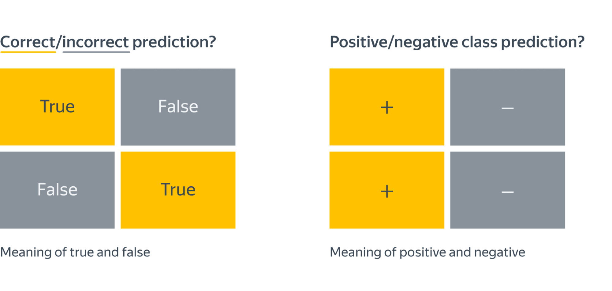
Заметим, что для каждого объекта в выборке возможно 4 ситуации:
- мы предсказали положительную метку и угадали. Будет относить такие объекты к true positive (TP) группе (true – потому что предсказали мы правильно, а positive – потому что предсказали положительную метку);
- мы предсказали положительную метку, но ошиблись в своём предсказании – false positive (FP) (false, потому что предсказание было неправильным);
- мы предсказали отрицательную метку и угадали – true negative (TN);
- и наконец, мы предсказали отрицательную метку, но ошиблись – false negative (FN). Для удобства все эти 4 числа изображают в виде таблицы, которую называют confusion matrix (матрицей ошибок):
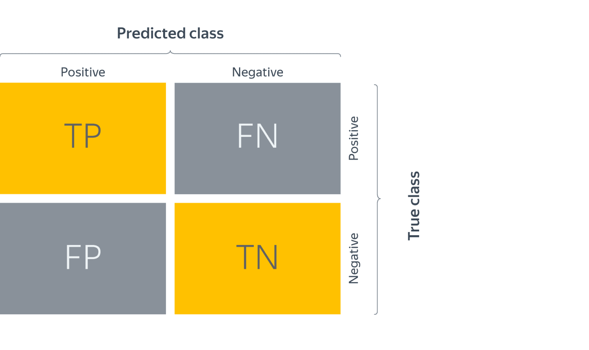
Не волнуйтесь, если первое время эти обозначения будут сводить вас с ума (будем откровенны, даже профи со стажем в них порой путаются), однако логика за ними достаточно простая: первая часть названия группы показывает угадали ли мы с классом, а вторая – какой класс мы предсказали.
Пример
Попробуем воспользоваться введёнными метриками в боевом примере: сравним работу нескольких моделей классификации на Breast cancer wisconsin (diagnostic) dataset.
Объектами выборки являются фотографии биопсии грудных опухолей. С их помощью было сформировано признаковое описание, которое заключается в характеристиках ядер клеток (таких как радиус ядра, его текстура, симметричность). Положительным классом в такой постановке будут злокачественные опухоли, а отрицательным – доброкачественные.
Модель 1. Константное предсказание.
Решение задачи начнём с самого простого классификатора, который выдаёт на каждом объекте константное предсказание – самый часто встречающийся класс.
Зачем вообще замерять качество на такой модели?При разработке модели машинного обучения для проекта всегда желательно иметь некоторую baseline модель. Так нам будет легче проконтролировать, что наша более сложная модель действительно дает нам прирост качества.
from sklearn.datasets
import load_breast_cancer
the_data = load_breast_cancer()

# 0 – "доброкачественный"
# 1 – "злокачественный"
relabeled_target = 1 - the_data["target"]

from sklearn.model_selection import train_test_split
X = the_data["data"]
y = relabeled_target
X_train, X_test, y_train, y_test = train_test_split(X, y, random_state=0)

from sklearn.dummy import DummyClassifier
dc_mf = DummyClassifier(strategy="most_frequent")
dc_mf.fit(X_train, y_train)

from sklearn.metrics import confusion_matrix
y_true = y_test y_pred = dc_mf.predict(X_test)
dc_mf_tn, dc_mf_fp, dc_mf_fn, dc_mf_tp = confusion_matrix(y_true, y_pred, labels = [0, 1]).ravel()
| Прогнозируемый класс + | Прогнозируемый класс — | |
|---|---|---|
| Истинный класс + | TP = 0 | FN = 53 |
| Истинный класс — | FP = 0 | TN = 90 |
Обучающие данные таковы, что наш dummy-классификатор все объекты записывает в отрицательный класс, то есть признаёт все опухоли доброкачественными. Такой наивный подход позволяет нам получить минимальный штраф за FP (действительно, нельзя ошибиться в предсказании, если положительный класс вообще не предсказывается), но и максимальный штраф за FN (в эту группу попадут все злокачественные опухоли).
Модель 2. Случайный лес.
Настало время воспользоваться всем арсеналом моделей машинного обучения, и начнём мы со случайного леса.
from sklearn.ensemble import RandomForestClassifier
rfc = RandomForestClassifier()
rfc.fit(X_train, y_train)
y_true = y_test
y_pred = rfc.predict(X_test)
rfc_tn, rfc_fp, rfc_fn, rfc_tp = confusion_matrix(y_true, y_pred, labels = [0, 1]).ravel()
| Прогнозируемый класс + | Прогнозируемый класс — | |
|---|---|---|
| Истинный класс + | TP = 52 | FN = 1 |
| Истинный класс — | FP = 4 | TN = 86 |
Можно сказать, что этот классификатор чему-то научился, т.к. главная диагональ матрицы стала содержать все объекты из отложенной выборки, за исключением 4 + 1 = 5 объектов (сравните с 0 + 53 объектами dummy-классификатора, все опухоли объявляющего доброкачественными).
Отметим, что вычисляя долю недиагональных элементов, мы приходим к метрике error rate, о которой мы говорили в самом начале:
$$text{Error rate} = frac{FP + FN}{ TP + TN + FP + FN}$$
тогда как доля объектов, попавших на главную диагональ – это как раз таки accuracy:
$$text{Accuracy} = frac{TP + TN}{ TP + TN + FP + FN}$$
Модель 3. Метод опорных векторов.
Давайте построим еще один классификатор на основе линейного метода опорных векторов.
Не забудьте привести признаки к единому масштабу, иначе численный алгоритм не сойдется к решению и мы получим гораздо более плохо работающее решающее правило. Попробуйте проделать это упражнение.
from sklearn.svm import LinearSVC
from sklearn.preprocessing import StandardScaler
ss = StandardScaler() ss.fit(X_train)
scaled_linsvc = LinearSVC(C=0.01,random_state=42)
scaled_linsvc.fit(ss.transform(X_train), y_train)
y_true = y_test
y_pred = scaled_linsvc.predict(ss.transform(X_test))
tn, fp, fn, tp = confusion_matrix(y_true, y_pred, labels = [0, 1]).ravel()
| Прогнозируемый класс + | Прогнозируемый класс — | |
|---|---|---|
| Истинный класс + | TP = 50 | FN = 3 |
| Истинный класс — | FP = 1 | TN = 89 |
Сравним результаты
Легко заметить, что каждая из двух моделей лучше классификатора-пустышки, однако давайте попробуем сравнить их между собой. С точки зрения error rate модели практически одинаковы: 5/143 для леса против 4/143 для SVM.
Посмотрим на структуру ошибок чуть более внимательно: лес – (FP = 4, FN = 1), SVM – (FP = 1, FN = 3). Какая из моделей предпочтительнее?
Замечание: Мы сравниваем несколько классификаторов на основании их предсказаний на отложенной выборке. Насколько ошибки данных классификаторов зависят от разбиения исходного набора данных? Иногда в процессе оценки качества мы будем получать модели, чьи показатели эффективности будут статистически неразличимыми.
Пусть мы учли предыдущее замечание и эти модели действительно статистически значимо ошибаются в разную сторону. Мы встретились с очевидной вещью: на матрицах нет отношения порядка. Когда мы сравнивали dummy-классификатор и случайный лес с помощью Accuracy, мы всю сложную структуру ошибок свели к одному числу, т.к. на вещественных числах отношение порядка есть. Сводить оценку модели к одному числу очень удобно, однако не стоит забывать, что у вашей модели есть много аспектов качества.
Что же всё-таки важнее уменьшить: FP или FN? Вернёмся к задаче: FP – доля доброкачественных опухолей, которым ошибочно присваивается метка злокачественной, а FN – доля злокачественных опухолей, которые классификатор пропускает. В такой постановке становится понятно, что при сравнении выиграет модель с меньшим FN (то есть лес в нашем примере), ведь каждая не обнаруженная опухоль может стоить человеческой жизни.
Рассмотрим теперь другую задачу: по данным о погоде предсказать, будет ли успешным запуск спутника. FN в такой постановке – это ошибочное предсказание неуспеха, то есть не более, чем упущенный шанс (если вас, конечно не уволят за срыв сроков). С FP всё серьёзней: если вы предскажете удачный запуск спутника, а на деле он потерпит крушение из-за погодных условий, то ваши потери будут в разы существеннее.
Итак, из примеров мы видим, что в текущем виде введенная нами доля ошибочных классификаций не даст нам возможности учесть неравную важность FP и FN. Поэтому введем две новые метрики: точность и полноту.
Точность и полнота
Accuracy — это метрика, которая характеризует качество модели, агрегированное по всем классам. Это полезно, когда классы для нас имеют одинаковое значение. В случае, если это не так, accuracy может быть обманчивой.
Рассмотрим ситуацию, когда положительный класс это событие редкое. Возьмем в качестве примера поисковую систему — в нашем хранилище хранятся миллиарды документов, а релевантных к конкретному поисковому запросу на несколько порядков меньше.
Пусть мы хотим решить задачу бинарной классификации «документ d релевантен по запросу q». Благодаря большому дисбалансу, Accuracy dummy-классификатора, объявляющего все документы нерелевантными, будет близка к единице. Напомним, что $text{Accuracy} = frac{TP + TN}{TP + TN + FP + FN}$, и в нашем случае высокое значение метрики будет обеспечено членом TN, в то время для пользователей более важен высокий TP.
Поэтому в случае ассиметрии классов, можно использовать метрики, которые не учитывают TN и ориентируются на TP.
Если мы рассмотрим долю правильно предсказанных положительных объектов среди всех объектов, предсказанных положительным классом, то мы получим метрику, которая называется точностью (precision)
$$color{#348FEA}{text{Precision} = frac{TP}{TP + FP}}$$
Интуитивно метрика показывает долю релевантных документов среди всех найденных классификатором. Чем меньше ложноположительных срабатываний будет допускать модель, тем больше будет её Precision.
Если же мы рассмотрим долю правильно найденных положительных объектов среди всех объектов положительного класса, то мы получим метрику, которая называется полнотой (recall)
$$color{#348FEA}{text{Recall} = frac{TP}{TP + FN}}$$
Интуитивно метрика показывает долю найденных документов из всех релевантных. Чем меньше ложно отрицательных срабатываний, тем выше recall модели.
Например, в задаче предсказания злокачественности опухоли точность показывает, сколько из определённых нами как злокачественные опухолей действительно являются злокачественными, а полнота – какую долю злокачественных опухолей нам удалось выявить.
Хорошее понимание происходящего даёт следующая картинка: 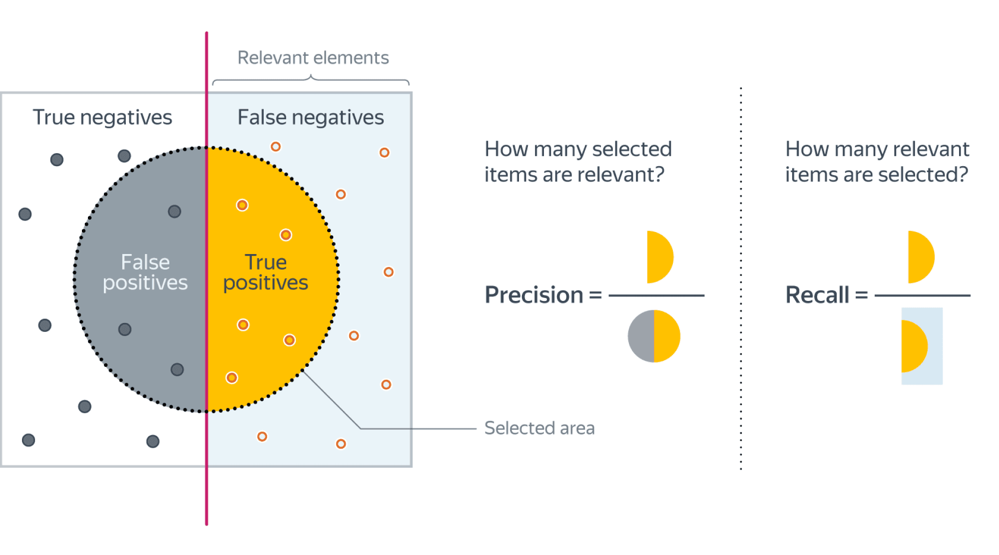 (источник картинки)
Recall@k, Precision@k
Метрики Recall и Precision хорошо подходят для задачи поиска «документ d релевантен запросу q», когда из списка рекомендованных алгоритмом документов нас интересует только первый. Но не всегда алгоритм машинного обучения вынужден работать в таких жестких условиях. Может быть такое, что вполне достаточно, что релевантный документ попал в первые k рекомендованных. Например, в интерфейсе выдачи первые три подсказки видны всегда одновременно и вообще не очень понятно, какой у них порядок. Тогда более честной оценкой качества алгоритма будет «в выдаче D размера k по запросу q нашлись релевантные документы». Для расчёта метрики по всей выборке объединим все выдачи и рассчитаем precision, recall как обычно подокументно.
F1-мера
Как мы уже отмечали ранее, модели очень удобно сравнивать, когда их качество выражено одним числом. В случае пары Precision-Recall существует популярный способ скомпоновать их в одну метрику — взять их среднее гармоническое. Данный показатель эффективности исторически носит название F1-меры (F1-measure).
$$
color{#348FEA}{F_1 = frac{2}{frac{1}{Recall} + frac{1}{Precision}}} = $$
$$ = 2 frac{Recall cdot Precision }{Recall + Precision} = frac
{TP} {TP + frac{FP + FN}{2}}
$$
Стоит иметь в виду, что F1-мера предполагает одинаковую важность Precision и Recall, если одна из этих метрик для вас приоритетнее, то можно воспользоваться $F_{beta}$ мерой:
$$
F_{beta} = (beta^2 + 1) frac{Recall cdot Precision }{Recall + beta^2Precision}
$$
Бинарная классификация: вероятности классов
Многие модели бинарной классификации устроены так, что класс объекта получается бинаризацией выхода классификатора по некоторому фиксированному порогу:
$$fleft(x ; w, w_{0}right)=mathbb{I}left[g(x, w) > w_{0}right].$$
Например, модель логистической регрессии возвращает оценку вероятности принадлежности примера к положительному классу. Другие модели бинарной классификации обычно возвращают произвольные вещественные значения, но существуют техники, называемые калибровкой классификатора, которые позволяют преобразовать предсказания в более или менее корректную оценку вероятности принадлежности к положительному классу.
Как оценить качество предсказываемых вероятностей, если именно они являются нашей конечной целью? Общепринятой мерой является логистическая функция потерь, которую мы изучали раньше, когда говорили об устройстве некоторых методов классификации (например уже упоминавшейся логистической регрессии).
Если же нашей целью является построение прогноза в терминах метки класса, то нам нужно учесть, что в зависимости от порога мы будем получать разные предсказания и разное качество на отложенной выборке. Так, чем ниже порог отсечения, тем больше объектов модель будет относить к положительному классу. Как в этом случае оценить качество модели?
AUC
Пусть мы хотим учитывать ошибки на объектах обоих классов. При уменьшении порога отсечения мы будем находить (правильно предсказывать) всё большее число положительных объектов, но также и неправильно предсказывать положительную метку на всё большем числе отрицательных объектов. Естественным кажется ввести две метрики TPR и FPR:
TPR (true positive rate) – это полнота, доля положительных объектов, правильно предсказанных положительными:
$$ TPR = frac{TP}{P} = frac{TP}{TP + FN} $$
FPR (false positive rate) – это доля отрицательных объектов, неправильно предсказанных положительными:
$$FPR = frac{FP}{N} = frac{FP}{FP + TN}$$
Обе эти величины растут при уменьшении порога. Кривая в осях TPR/FPR, которая получается при варьировании порога, исторически называется ROC-кривой (receiver operating characteristics curve, сокращённо ROC curve). Следующий график поможет вам понять поведение ROC-кривой.
Желтая и синяя кривые показывают распределение предсказаний классификатора на объектах положительного и отрицательного классов соответственно. То есть значения на оси X (на графике с двумя гауссианами) мы получаем из классификатора. Если классификатор идеальный (две кривые разделимы по оси X), то на правом графике мы получаем ROC-кривую (0,0)->(0,1)->(1,1) (убедитесь сами!), площадь под которой равна 1. Если классификатор случайный (предсказывает одинаковые метки положительным и отрицательным объектам), то мы получаем ROC-кривую (0,0)->(1,1), площадь под которой равна 0.5. Поэкспериментируйте с разными вариантами распределения предсказаний по классам и посмотрите, как меняется ROC-кривая.
Чем лучше классификатор разделяет два класса, тем больше площадь (area under curve) под ROC-кривой – и мы можем использовать её в качестве метрики. Эта метрика называется AUC и она работает благодаря следующему свойству ROC-кривой:
AUC равен доле пар объектов вида (объект класса 1, объект класса 0), которые алгоритм верно упорядочил, т.е. предсказание классификатора на первом объекте больше:
$$
color{#348FEA}{operatorname{AUC} = frac{sumlimits_{i = 1}^{N} sumlimits_{j = 1}^{N}mathbb{I}[y_i < y_j] I^{prime}[f(x_{i}) < f(x_{j})]}{sumlimits_{i = 1}^{N} sumlimits_{j = 1}^{N}mathbb{I}[y_i < y_j]}}
$$
$$
I^{prime}left[f(x_{i}) < f(x_{j})right]=
left{
begin{array}{ll}
0, & f(x_{i}) > f(x_{j}) \
0.5 & f(x_{i}) = f(x_{j}) \
1, & f(x_{i}) < f(x_{j})
end{array}
right.
$$
$$
Ileft[y_{i}< y_{j}right]=
left{
begin{array}{ll}
0, & y_{i} geq y_{j} \
1, & y_{i} < y_{j}
end{array}
right.
$$
Чтобы детальнее разобраться, почему это так, советуем вам обратиться к материалам А.Г.Дьяконова.
В каких случаях лучше отдать предпочтение этой метрике? Рассмотрим следующую задачу: некоторый сотовый оператор хочет научиться предсказывать, будет ли клиент пользоваться его услугами через месяц. На первый взгляд кажется, что задача сводится к бинарной классификации с метками 1, если клиент останется с компанией и $0$ – иначе.
Однако если копнуть глубже в процессы компании, то окажется, что такие метки практически бесполезны. Компании скорее интересно упорядочить клиентов по вероятности прекращения обслуживания и в зависимости от этого применять разные варианты удержания: кому-то прислать скидочный купон от партнёра, кому-то предложить скидку на следующий месяц, а кому-то и новый тариф на особых условиях.
Таким образом, в любой задаче, где нам важна не метка сама по себе, а правильный порядок на объектах, имеет смысл применять AUC.
Утверждение выше может вызывать у вас желание использовать AUC в качестве метрики в задачах ранжирования, но мы призываем вас быть аккуратными.
ПодробнееУтверждение выше может вызывать у вас желание использовать AUC в качестве метрики в задачах ранжирования, но мы призываем вас быть аккуратными.» details=»Продемонстрируем это на следующем примере: пусть наша выборка состоит из $9100$ объектов класса $0$ и $10$ объектов класса $1$, и модель расположила их следующим образом:
$$underbrace{0 dots 0}_{9000} ~ underbrace{1 dots 1}_{10} ~ underbrace{0 dots 0}_{100}$$
Тогда AUC будет близка к единице: количество пар правильно расположенных объектов будет порядка $90000$, в то время как общее количество пар порядка $91000$.
Однако самыми высокими по вероятности положительного класса будут совсем не те объекты, которые мы ожидаем.
Average Precision
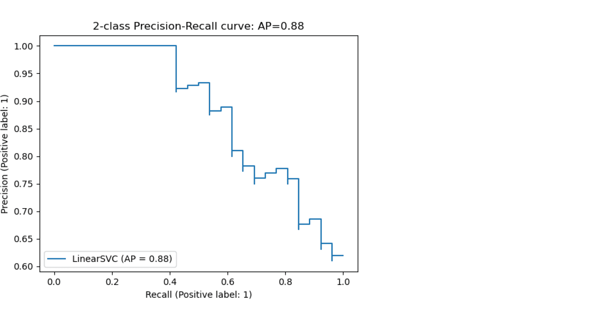
Будем постепенно уменьшать порог бинаризации. При этом полнота будет расти от $0$ до $1$, так как будет увеличиваться количество объектов, которым мы приписываем положительный класс (а количество объектов, на самом деле относящихся к положительному классу, очевидно, меняться не будет). Про точность же нельзя сказать ничего определённого, но мы понимаем, что скорее всего она будет выше при более высоком пороге отсечения (мы оставим только объекты, в которых модель «уверена» больше всего). Варьируя порог и пересчитывая значения Precision и Recall на каждом пороге, мы получим некоторую кривую примерно следующего вида:
 (источник картинки)
Рассмотрим среднее значение точности (оно равно площади под кривой точность-полнота):
$$ text { AP }=int_{0}^{1} p(r) d r$$
Получим показатель эффективности, который называется average precision. Как в случае матрицы ошибок мы переходили к скалярным показателям эффективности, так и в случае с кривой точность-полнота мы охарактеризовали ее в виде числа.
Многоклассовая классификация
Если классов становится больше двух, расчёт метрик усложняется. Если задача классификации на $K$ классов ставится как $K$ задач об отделении класса $i$ от остальных ($i=1,ldots,K$), то для каждой из них можно посчитать свою матрицу ошибок. Затем есть два варианта получения итогового значения метрики из $K$ матриц ошибок:
- Усредняем элементы матрицы ошибок (TP, FP, TN, FN) между бинарными классификаторами, например $TP = frac{1}{K}sum_{i=1}^{K}TP_i$. Затем по одной усреднённой матрице ошибок считаем Precision, Recall, F-меру. Это называют микроусреднением.
- Считаем Precision, Recall для каждого классификатора отдельно, а потом усредняем. Это называют макроусреднением.
Порядок усреднения влияет на результат в случае дисбаланса классов. Показатели TP, FP, FN — это счётчики объектов. Пусть некоторый класс обладает маленькой мощностью (обозначим её $M$). Тогда значения TP и FN при классификации этого класса против остальных будут не больше $M$, то есть тоже маленькие. Про FP мы ничего уверенно сказать не можем, но скорее всего при дисбалансе классов классификатор не будет предсказывать редкий класс слишком часто, потому что есть большая вероятность ошибиться. Так что FP тоже мало. Поэтому усреднение первым способом сделает вклад маленького класса в общую метрику незаметным. А при усреднении вторым способом среднее считается уже для нормированных величин, так что вклад каждого класса будет одинаковым.
Рассмотрим пример. Пусть есть датасет из объектов трёх цветов: желтого, зелёного и синего. Желтого и зелёного цветов почти поровну — 21 и 20 объектов соответственно, а синих объектов всего 4.
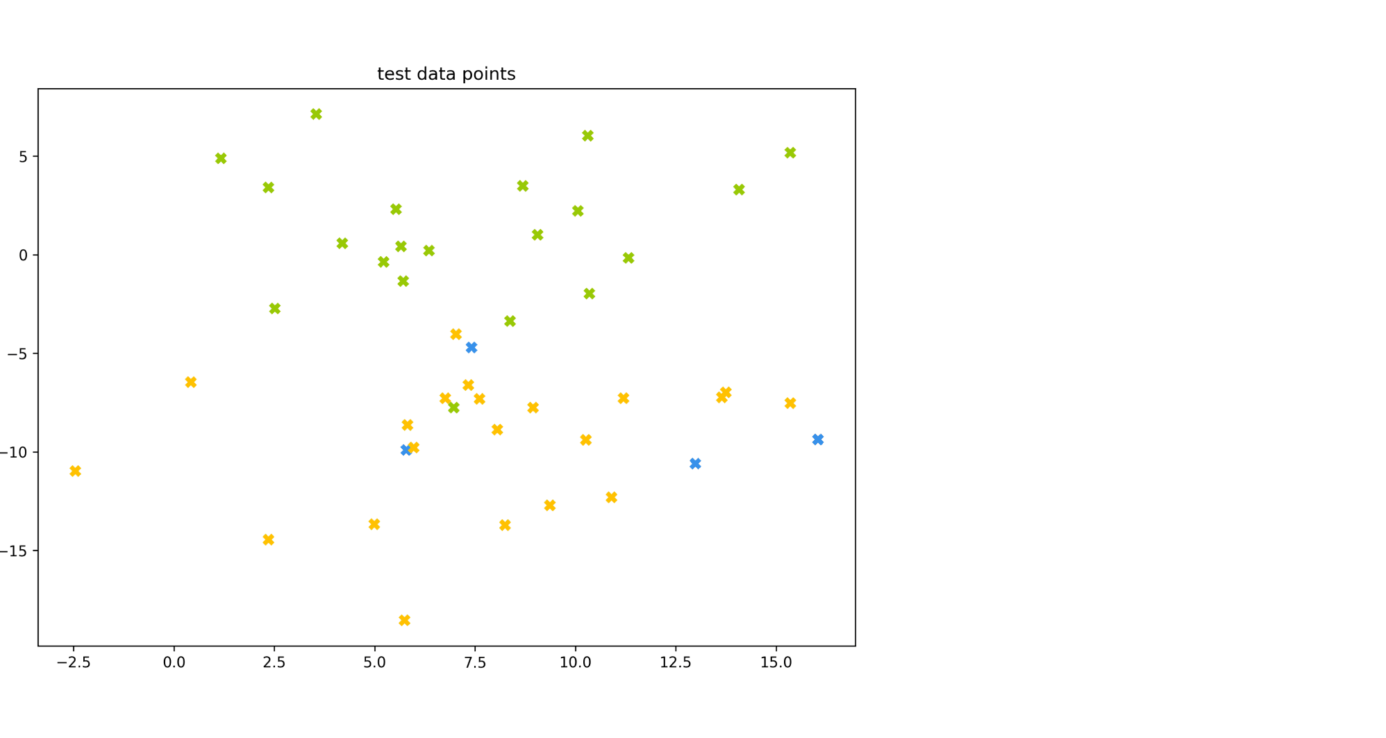
Модель по очереди для каждого цвета пытается отделить объекты этого цвета от объектов оставшихся двух цветов. Результаты классификации проиллюстрированы матрицей ошибок. Модель «покрасила» в жёлтый 25 объектов, 20 из которых были действительно жёлтыми (левый столбец матрицы). В синий был «покрашен» только один объект, который на самом деле жёлтый (средний столбец матрицы). В зелёный — 19 объектов, все на самом деле зелёные (правый столбец матрицы).
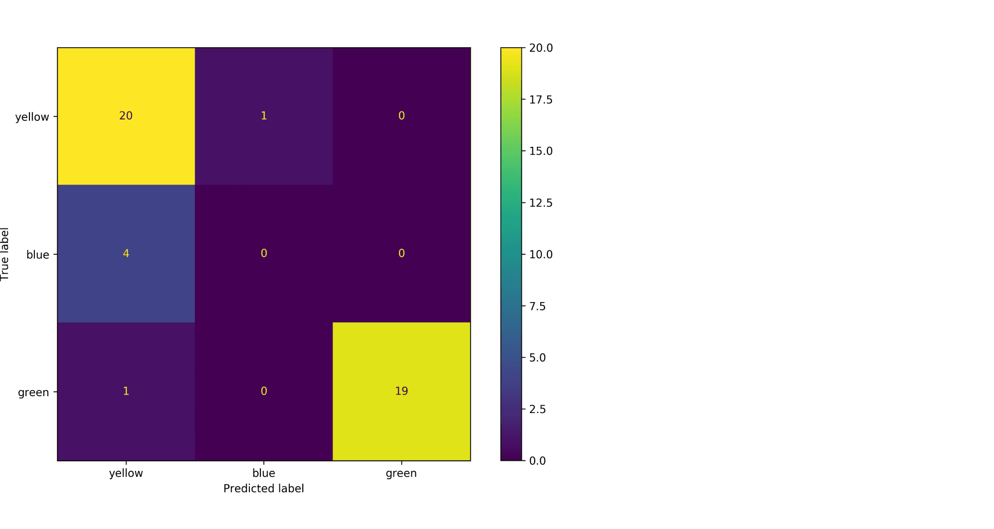
Посчитаем Precision классификации двумя способами:
- С помощью микроусреднения получаем $$
text{Precision} = frac{dfrac{1}{3}left(20 + 0 + 19right)}{dfrac{1}{3}left(20 + 0 + 19right) + dfrac{1}{3}left(5 + 1 + 0right)} = 0.87
$$ - С помощью макроусреднения получаем $$
text{Precision} = dfrac{1}{3}left( frac{20}{20 + 5} + frac{0}{0 + 1} + frac{19}{19 + 0}right) = 0.6
$$
Видим, что макроусреднение лучше отражает тот факт, что синий цвет, которого в датасете было совсем мало, модель практически игнорирует.
Как оптимизировать метрики классификации?
Пусть мы выбрали, что метрика качества алгоритма будет $F(a(X), Y)$. Тогда мы хотим обучить модель так, чтобы $F$ на валидационной выборке была минимальная/максимальная. Лучший способ добиться минимизации метрики $F$ — оптимизировать её напрямую, то есть выбрать в качестве функции потерь ту же $F(a(X), Y)$. К сожалению, это не всегда возможно. Рассмотрим, как оптимизировать метрики иначе.
Метрики precision и recall невозможно оптимизировать напрямую, потому что эти метрики нельзя рассчитать на одном объекте, а затем усреднить. Они зависят от того, какими были правильная метка класса и ответ алгоритма на всех объектах. Чтобы понять, как оптимизировать precision, recall, рассмотрим, как расчитать эти метрики на отложенной выборке. Пусть модель обучена на стандартную для классификации функцию потерь (LogLoss). Для получения меток класса специалист по машинному обучению сначала применяет на объектах модель и получает вещественные предсказания модели ($p_i in left(0, 1right)$). Затем предсказания бинаризуются по порогу, выбранному специалистом: если предсказание на объекте больше порога, то метка класса 1 (или «положительная»), если меньше — 0 (или «отрицательная»). Рассмотрим, что будет с метриками precision, recall в крайних положениях порога.
- Пусть порог равен нулю. Тогда всем объектам будет присвоена положительная метка. Следовательно, все объекты будут либо TP, либо FP, потому что отрицательных предсказаний нет, $TP + FP = N$, где $N$ — размер выборки. Также все объекты, у которых метка на самом деле 1, попадут в TP. По формуле точность $text{Precision} = frac{TP}{TP + FP} = frac1N sum_{i = 1}^N mathbb{I} left[ y_i = 1 right]$ равна среднему таргету в выборке. А полнота $text{Recall} = frac{TP}{TP + FN} = frac{TP}{TP + 0} = 1$ равна единице.
- Пусть теперь порог равен единице. Тогда ни один объект не будет назван положительным, $TP = FP = 0$. Все объекты с меткой класса 1 попадут в FN. Если есть хотя бы один такой объект, то есть $FN ne 0$, будет верна формула $text{Recall} = frac{TP}{TP + FN} = frac{0}{0+ FN} = 0$. То есть при пороге единица, полнота равна нулю. Теперь посмотрим на точность. Формула для Precision состоит только из счётчиков положительных ответов модели (TP, FP). При единичном пороге они оба равны нулю, $text{Precision} = frac{TP}{TP + FP} = frac{0}{0 + 0}$то есть при единичном пороге точность неопределена. Пусть мы отступили чуть-чуть назад по порогу, чтобы хотя бы несколько объектов были названы моделью положительными. Скорее всего это будут самые «простые» объекты, которые модель распознает хорошо, потому что её предсказание близко к единице. В этом предположении $FP approx 0$. Тогда точность $text{Precision} = frac{TP}{TP + FP} approx frac{TP}{TP + 0} approx 1$ будет близка к единице.
Изменяя порог, между крайними положениями, получим графики Precision и Recall, которые выглядят как-то так:
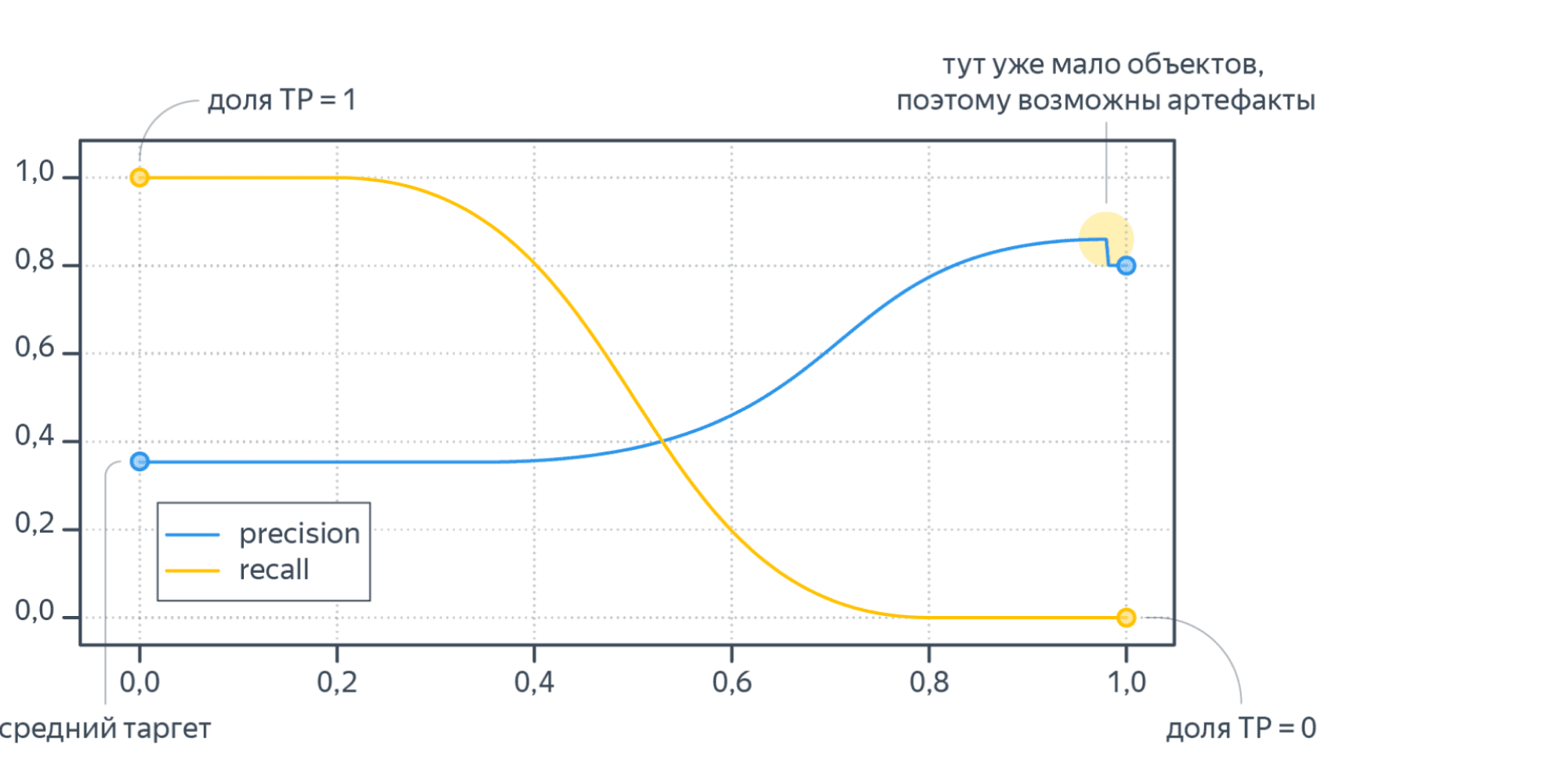
Recall меняется от единицы до нуля, а Precision от среднего тагрета до какого-то другого значения (нет гарантий, что график монотонный).
Итого оптимизация precision и recall происходит так:
- Модель обучается на стандартную функцию потерь (например, LogLoss).
- Используя вещественные предсказания на валидационной выборке, перебирая разные пороги от 0 до 1, получаем графики метрик в зависимости от порога.
- Выбираем нужное сочетание точности и полноты.
Пусть теперь мы хотим максимизировать метрику AUC. Стандартный метод оптимизации, градиентный спуск, предполагает, что функция потерь дифференцируема. AUC этим качеством не обладает, то есть мы не можем оптимизировать её напрямую. Поэтому для метрики AUC приходится изменять оптимизационную задачу. Метрика AUC считает долю верно упорядоченных пар. Значит от исходной выборки можно перейти к выборке упорядоченных пар объектов. На этой выборке ставится задача классификации: метка класса 1 соответствует правильно упорядоченной паре, 0 — неправильно. Новой метрикой становится accuracy — доля правильно классифицированных объектов, то есть доля правильно упорядоченных пар. Оптимизировать accuracy можно по той же схеме, что и precision, recall: обучаем модель на LogLoss и предсказываем вероятности положительной метки у объекта выборки, считаем accuracy для разных порогов по вероятности и выбираем понравившийся.
Регрессия
В задачах регрессии целевая метка у нас имеет потенциально бесконечное число значений. И природа этих значений, обычно, связана с каким-то процессом измерений:
- величина температуры в определенный момент времени на метеостанции
- количество прочтений статьи на сайте
- количество проданных бананов в конкретном магазине, сети магазинов или стране
- дебит добывающей скважины на нефтегазовом месторождении за месяц и т.п.
Мы видим, что иногда метка это целое число, а иногда произвольное вещественное число. Обычно случаи целочисленных меток моделируют так, словно это просто обычное вещественное число. При таком подходе может оказаться так, что модель A лучше модели B по некоторой метрике, но при этом предсказания у модели A могут быть не целыми. Если в бизнес-задаче ожидается именно целочисленный ответ, то и оценивать нужно огрубление.
Общая рекомендация такова: оценивайте весь каскад решающих правил: и те «внутренние», которые вы получаете в результате обучения, и те «итоговые», которые вы отдаёте бизнес-заказчику.
Например, вы можете быть удовлетворены, что стали ошибаться не во втором, а только в третьем знаке после запятой при предсказании погоды. Но сами погодные данные измеряются с точностью до десятых долей градуса, а пользователь и вовсе может интересоваться лишь целым числом градусов.
Итак, напомним постановку задачи регрессии: нам нужно по обучающей выборке ${(x_i, y_i)}_{i=1}^N$, где $y_i in mathbb{R}$ построить модель f(x).
Величину $ e_i = f(x_i) — y_i $ называют ошибкой на объекте i или регрессионным остатком.
Весь набор ошибок на отложенной выборке может служить аналогом матрицы ошибок из задачи классификации. А именно, когда мы рассматриваем две разные модели, то, глядя на то, как и на каких объектах они ошиблись, мы можем прийти к выводу, что для решения бизнес-задачи нам выгоднее взять ту или иную модель. И, аналогично со случаем бинарной классификации, мы можем начать строить агрегаты от вектора ошибок, получая тем самым разные метрики.
MSE, RMSE, $R^2$
MSE – одна из самых популярных метрик в задаче регрессии. Она уже знакома вам, т.к. применяется в качестве функции потерь (или входит в ее состав) во многих ранее рассмотренных методах.
$$ MSE(y^{true}, y^{pred}) = frac1Nsum_{i=1}^{N} (y_i — f(x_i))^2 $$
Иногда для того, чтобы показатель эффективности MSE имел размерность исходных данных, из него извлекают квадратный корень и получают показатель эффективности RMSE.
MSE неограничен сверху, и может быть нелегко понять, насколько «хорошим» или «плохим» является то или иное его значение. Чтобы появились какие-то ориентиры, делают следующее:
-
Берут наилучшее константное предсказание с точки зрения MSE — среднее арифметическое меток $bar{y}$. При этом чтобы не было подглядывания в test, среднее нужно вычислять по обучающей выборке
-
Рассматривают в качестве показателя ошибки:
$$ R^2 = 1 — frac{sum_{i=1}^{N} (y_i — f(x_i))^2}{sum_{i=1}^{N} (y_i — bar{y})^2}.$$
У идеального решающего правила $R^2$ равен $1$, у наилучшего константного предсказания он равен $0$ на обучающей выборке. Можно заметить, что $R^2$ показывает, какая доля дисперсии таргетов (знаменатель) объяснена моделью.
MSE квадратично штрафует за большие ошибки на объектах. Мы уже видели проявление этого при обучении моделей методом минимизации квадратичных ошибок – там это проявлялось в том, что модель старалась хорошо подстроиться под выбросы.
Пусть теперь мы хотим использовать MSE для оценки наших регрессионных моделей. Если большие ошибки для нас действительно неприемлемы, то квадратичный штраф за них — очень полезное свойство (и его даже можно усиливать, повышая степень, в которую мы возводим ошибку на объекте). Однако если в наших тестовых данных присутствуют выбросы, то нам будет сложно объективно сравнить модели между собой: ошибки на выбросах будет маскировать различия в ошибках на основном множестве объектов.
Таким образом, если мы будем сравнивать две модели при помощи MSE, у нас будет выигрывать та модель, у которой меньше ошибка на объектах-выбросах, а это, скорее всего, не то, чего требует от нас наша бизнес-задача.
История из жизни про бананы и квадратичный штраф за ошибкуИз-за неверно введенных данных метка одного из объектов оказалась в 100 раз больше реального значения. Моделировалась величина при помощи градиентного бустинга над деревьями решений. Функция потерь была MSE.
Однажды уже во время эксплуатации случилось ч.п.: у нас появились предсказания, в 100 раз превышающие допустимые из соображений физического смысла значения. Представьте себе, например, что вместо обычных 4 ящиков бананов система предлагала поставить в магазин 400. Были распечатаны все деревья из ансамбля, и мы увидели, что постепенно число ящиков действительно увеличивалось до прогнозных 400.
Было решено проверить гипотезу, что был выброс в данных для обучения. Так оно и оказалось: всего одна точка давала такую потерю на объекте, что алгоритм обучения решил, что лучше переобучиться под этот выброс, чем смириться с большим штрафом на этом объекте. А в эксплуатации у нас возникли точки, которые плюс-минус попадали в такие же листья ансамбля, что и объект-выброс.
Избежать такого рода проблем можно двумя способами: внимательнее контролируя качество данных или адаптировав функцию потерь.
Аналогично, можно поступать и в случае, когда мы разрабатываем метрику качества: менее жёстко штрафовать за большие отклонения от истинного таргета.
MAE
Использовать RMSE для сравнения моделей на выборках с большим количеством выбросов может быть неудобно. В таких случаях прибегают к также знакомой вам в качестве функции потери метрике MAE (mean absolute error):
$$ MAE(y^{true}, y^{pred}) = frac{1}{N}sum_{i=1}^{N} left|y_i — f(x_i)right| $$
Метрики, учитывающие относительные ошибки
И MSE и MAE считаются как сумма абсолютных ошибок на объектах.
Рассмотрим следующую задачу: мы хотим спрогнозировать спрос товаров на следующий месяц. Пусть у нас есть два продукта: продукт A продаётся в количестве 100 штук, а продукт В в количестве 10 штук. И пусть базовая модель предсказывает количество продаж продукта A как 98 штук, а продукта B как 8 штук. Ошибки на этих объектах добавляют 4 штрафных единицы в MAE.
И есть 2 модели-кандидата на улучшение. Первая предсказывает товар А 99 штук, а товар B 8 штук. Вторая предсказывает товар А 98 штук, а товар B 9 штук.
Обе модели улучшают MAE базовой модели на 1 единицу. Однако, с точки зрения бизнес-заказчика вторая модель может оказаться предпочтительнее, т.к. предсказание продажи редких товаров может быть приоритетнее. Один из способов учесть такое требование – рассматривать не абсолютную, а относительную ошибку на объектах.
MAPE, SMAPE
Когда речь заходит об относительных ошибках, сразу возникает вопрос: что мы будем ставить в знаменатель?
В метрике MAPE (mean absolute percentage error) в знаменатель помещают целевое значение:
$$ MAPE(y^{true}, y^{pred}) = frac{1}{N} sum_{i=1}^{N} frac{ left|y_i — f(x_i)right|}{left|y_iright|} $$
С особым случаем, когда в знаменателе оказывается $0$, обычно поступают «инженерным» способом: или выдают за непредсказание $0$ на таком объекте большой, но фиксированный штраф, или пытаются застраховаться от подобного на уровне формулы и переходят к метрике SMAPE (symmetric mean absolute percentage error):
$$ SMAPE(y^{true}, y^{pred}) = frac{1}{N} sum_{i=1}^{N} frac{ 2 left|y_i — f(x_i)right|}{y_i + f(x_i)} $$
Если же предсказывается ноль, штраф считаем нулевым.
Таким переходом от абсолютных ошибок на объекте к относительным мы сделали объекты в тестовой выборке равнозначными: даже если мы делаем абсурдно большое предсказание, на фоне которого истинная метка теряется, мы получаем штраф за этот объект порядка 1 в случае MAPE и 2 в случае SMAPE.
WAPE
Как и любая другая метрика, MAPE имеет свои границы применимости: например, она плохо справляется с прогнозом спроса на товары с прерывистыми продажами. Рассмотрим такой пример:
| Понедельник | Вторник | Среда | |
|---|---|---|---|
| Прогноз | 55 | 2 | 50 |
| Продажи | 50 | 1 | 50 |
| MAPE | 10% | 100% | 0% |
Среднее MAPE – 36.7%, что не очень отражает реальную ситуацию, ведь два дня мы предсказывали с хорошей точностью. В таких ситуациях помогает WAPE (weighted average percentage error):
$$ WAPE(y^{true}, y^{pred}) = frac{sum_{i=1}^{N} left|y_i — f(x_i)right|}{sum_{i=1}^{N} left|y_iright|} $$
Если мы предсказываем идеально, то WAPE = 0, если все предсказания отдаём нулевыми, то WAPE = 1.
В нашем примере получим WAPE = 5.9%
RMSLE
Альтернативный способ уйти от абсолютных ошибок к относительным предлагает метрика RMSLE (root mean squared logarithmic error):
$$ RMSLE(y^{true}, y^{pred}| c) = sqrt{ frac{1}{N} sum_{i=1}^N left(vphantom{frac12}log{left(y_i + c right)} — log{left(f(x_i) + c right)}right)^2 } $$
где нормировочная константа $c$ вводится искусственно, чтобы не брать логарифм от нуля. Также по построению видно, что метрика пригодна лишь для неотрицательных меток.
Веса в метриках
Все вышеописанные метрики легко допускают введение весов для объектов. Если мы из каких-то соображений можем определить стоимость ошибки на объекте, можно брать эту величину в качестве веса. Например, в задаче предсказания спроса в качестве веса можно использовать стоимость объекта.
Доля предсказаний с абсолютными ошибками больше, чем d
Еще одним способом охарактеризовать качество модели в задаче регрессии является доля предсказаний с абсолютными ошибками больше заданного порога $d$:
$$frac{1}{N} sum_{i=1}^{N} mathbb{I}left[ left| y_i — f(x_i) right| > d right] $$
Например, можно считать, что прогноз погоды сбылся, если ошибка предсказания составила меньше 1/2/3 градусов. Тогда рассматриваемая метрика покажет, в какой доле случаев прогноз не сбылся.
Как оптимизировать метрики регрессии?
Пусть мы выбрали, что метрика качества алгоритма будет $F(a(X), Y)$. Тогда мы хотим обучить модель так, чтобы F на валидационной выборке была минимальная/максимальная. Аналогично задачам классификации лучший способ добиться минимизации метрики $F$ — выбрать в качестве функции потерь ту же $F(a(X), Y)$. К счастью, основные метрики для регрессии: MSE, RMSE, MAE можно оптимизировать напрямую. С формальной точки зрения MAE не дифференцируема, так как там присутствует модуль, чья производная не определена в нуле. На практике для этого выколотого случая в коде можно возвращать ноль.
Для оптимизации MAPE придётся изменять оптимизационную задачу. Оптимизацию MAPE можно представить как оптимизацию MAE, где объектам выборки присвоен вес $frac{1}{vert y_ivert}$.
I. Overview
This suite supports evaluation of diarization system output relative
to a reference diarization subject to the following conditions:
- both the reference and system diarizations are saved within Rich
Transcription Time Marked (RTTM) files - for any pair of recordings, the sets of speakers are disjoint
II. Dependencies
The following Python packages are required to run this software:
- Python >= 2.7.1* (https://www.python.org/)
- NumPy >= 1.6.1 (https://github.com/numpy/numpy)
- SciPy >= 0.17.0 (https://github.com/scipy/scipy)
- intervaltree >= 3.0.0 (https://pypi.python.org/pypi/intervaltree)
- tabulate >= 0.5.0 (https://pypi.python.org/pypi/tabulate)
- Tested with Python 2.7.X, 3.6.X, and 3.7.X.
III. Metrics
Diarization error rate
Following tradition in this area, we report diarization error rate (DER), which
is the sum of
- speaker error — percentage of scored time for which the wrong speaker id
is assigned within a speech region - false alarm speech — percentage of scored time for which a nonspeech
region is incorrectly marked as containing speech - missed speech — percentage of scored time for which a speech region is
incorrectly marked as not containing speech
As with word error rate, a score of zero indicates perfect performance and
higher scores (which may exceed 100) indicate poorer performance. For more
details, consult section 6.1 of the NIST RT-09 evaluation plan.
Jaccard error rate
We also report Jaccard error rate (JER), a metric introduced for DIHARD II that is based on the Jaccard index. The Jaccard index is a similarity
measure typically used to evaluate the output of image segmentation systems and
is defined as the ratio between the intersection and union of two segmentations.
To compute Jaccard error rate, an optimal mapping between reference and system
speakers is determined and for each pair the Jaccard index of their
segmentations is computed. The Jaccard error rate is then 1 minus the average
of these scores.
More concretely, assume we have N reference speakers and M system
speakers. An optimal mapping between speakers is determined using the
Hungarian algorithm so that each reference speaker is paired with at most one
system speaker and each system speaker with at most one reference speaker. Then,
for each reference speaker ref the speaker-specific Jaccard error rate is
(FA + MISS)/TOTAL, where:
TOTALis the duration of the union of reference and system speaker
segments; if the reference speaker was not paired with a system speaker, it is
the duration of all reference speaker segmentsFAis the total system speaker time not attributed to the reference
speaker; if the reference speaker was not paired with a system speaker, it is
0MISSis the total reference speaker time not attributed to the system
speaker; if the reference speaker was not paired with a system speaker, it is
equal toTOTAL
The Jaccard error rate then is the average of the speaker specific Jaccard error
rates.
JER and DER are highly correlated with JER typically being higher, especially in
recordings where one or more speakers is particularly dominant. Where it tends
to track DER is in outliers where the diarization is especially bad, resulting
in one or more unmapped system speakers whose speech is not then penalized. In
these cases, where DER can easily exceed 500%, JER will never exceed 100% and
may be far lower if the reference speakers are handled correctly. For this
reason, it may be useful to pair JER with another metric evaluating speech
detection and/or speaker overlap detection.
Clustering metrics
A third approach to system evaluation is convert both the reference and system
outputs to frame-level labels, then evaluate using one of many well-known
approaches for evaluating clustering performance. Each recording is converted to
a sequence of 10 ms frames, each of which is assigned a single label
corresponding to one of the following cases:
- the frame contains no speech
- the frame contains speech from a single speaker (one label per speaker
indentified) - the frame contains overlapping speech (one label for each element in the
powerset of speakers)
These frame-level labelings are then scored with the following metrics:
Goodman-Kruskal tau
Goodman-Kruskal tau is an asymmetric association measure dating back to work
by Leo Goodman and William Kruskal in the 1950s (Goodman and Kruskal, 1954).
For a reference labeling ref and a system labeling sys,
GKT(ref, sys) corresponds to the fraction of variability in sys that
can be explained by ref. Consequently, GKT(ref, sys) is 1 when ref
is perfectly predictive of sys and 0 when it is not predictive at all.
Correspondingly, GKT(sys, ref) is 1 when sys is perfectly predictive
of ref and 0 when lacking any predictive power.
B-cubed precision, recall, and F1
The B-cubed precision for a single frame assigned speaker S in the
reference diarization and C in the system diarization is the proportion of
frames assigned C that are also assigned S. Similarly, the B-cubed
recall for a frame is the proportion of all frames assigned S that are
also assigned C. The overall precision and recall, then, are just the mean
of the frame-level precision and recall measures and the overall F-1 their
harmonic mean. For additional details see Bagga and Baldwin (1998).
Information theoretic measures
We report four information theoretic measures:
H(ref|sys)— conditional conditional entropy in bits of the reference
labeling given the system labelingH(sys|ref)— conditional conditional entropy in bits of the system
labeling given the reference labelingMI— mutual information in bits between the reference and system
labelingsNMI— normalized mutual information between the reference and system
labelings; that is,MIscaled to the interval [0, 1]. In this case, the
normalization term used issqrt(H(ref)*H(sys)).
H(ref|sys) is the number of bits needed to describe the reference
labeling given that the system labeling is known and ranges from 0 in
the case that the system labeling is perfectly predictive of the reference
labeling to H(ref) in the case that the system labeling is not at
all predictive of the reference labeling. Similarly, H(sys|ref) measure
the number of bits required to describe the system labeling given the
reference labeling and ranges from 0 to H(sys).
MI is the number of bits shared by the reference and system labeling and
indicates the degree to which knowing either reduces uncertainty in the other.
It is related to conditional entropy and entropy as follows:
MI(ref, sys) = H(ref) - H(ref|sys) = H(sys) - H(sys|ref). NMI is
derived from MI by normalizing it to the interval [0, 1]. Multiple
normalizations are possible depending on the upper-bound for MI that is
used, but we report NMI normalized by sqrt(H(ref)*H(sys)).
IV. Scoring
To evaluate system output stored in RTTM files sys1.rttm,
sys2.rttm, … against a corresponding reference diarization stored in RTTM
files ref1.rttm, ref2.rttm, …:
python score.py -r ref1.rttm ref2.rttm ... -s sys1.rttm sys2.rttm ...
which will calculate and report the following metrics both overall and on
a per-file basis:
DER— diarization error rate (in percent)JER— Jaccard error rate (in percent)B3-Precision— B-cubed precisionB3-Recall— B-cubed recallB3-F1— B-cubed F1GKT(ref, sys)— Goodman-Kruskal tau in the direction of the reference
diarization to the system diarizationGKT(sys, ref)— Goodman-Kruskal tau in the direction of the system
diarization to the reference diarizationH(ref|sys)— conditional entropy in bits of the reference diarization
given the system diarizationH(sys|ref)— conditional entropy in bits of the system diarization
given the reference diarizationMI— mutual information in bitsNMI— normalized mutual information
Alternately, we could have specified the reference and system RTTM files via
script files of paths (one per line) using the -R and -S flags:
python score.py -R ref.scp -S sys.scp
By default the scoring regions for each file will be determined automatically
from the reference and speaker turns. However, it is possible to specify
explicit scoring regions using a NIST un-partitioned evaluation map (UEM) file and the -u flag. For instance, the following:
python score.py -u all.uem -R ref.scp -S sys.scp
will load the files to be scored plus scoring regions from all.uem, filter
out and warn about any speaker turns not present in those files, and trim the
remaining turns to the relevant scoring regions before computing the metrics
as before.
DER is scored using the NIST md-eval.pl tool with a default collar size of
0 ms and explicitly including regions that contain overlapping speech in the
reference diarization. If desired, this behavior can be altered using the
--collar and --ignore_overlaps flags. For instance
python score.py --collar 0.100 --ignore_overlaps -R ref.scp -S sys.scp
would compute DER using a 100 ms collar and with overlapped speech ignored.
All other metrics are computed off of frame-level labelings generated from the
reference and system speaker turns WITHOUT any use of collars. The default
frame step is 10 ms, which may be altered via the --step flag. For more
details, consult the docstrings within the scorelib.metrics module.
The overall and per-file results will be printed to STDOUT as a table; for
instance:
File                           DER    JER    B3-Precision    B3-Recall    B3-F1    GKT(ref, sys)    GKT(sys, ref)    H(ref|sys)    H(sys|ref)    MI    NMI
---------------------------  -----  -----  --------------  -----------  -------  ---------------  ---------------  ------------  ------------  ----  -----
CMU_20020319-1400_d01_NONE    6.10  20.10            0.91         1.00     0.95             1.00             0.88          0.22          0.00  2.66   0.96
ICSI_20000807-1000_d05_NONE  17.37  21.92            0.72         1.00     0.84             1.00             0.68          0.65          0.00  2.79   0.90
ICSI_20011030-1030_d02_NONE  13.06  25.61            0.80         0.95     0.87             0.95             0.80          0.54          0.11  5.10   0.94
LDC_20011116-1400_d06_NONE    5.64  16.10            0.95         0.89     0.92             0.85             0.93          0.10          0.27  1.87   0.91
LDC_20011116-1500_d07_NONE    1.69   2.00            0.96         0.96     0.96             0.95             0.95          0.14          0.12  2.39   0.95
NIST_20020305-1007_d01_NONE  42.05  53.38            0.51         0.95     0.66             0.93             0.44          1.58          0.11  2.13   0.74
*** OVERALL ***              14.31  26.75            0.81         0.96     0.88             0.96             0.80          0.55          0.10  5.45   0.94
Some basic control of the formatting of this table is possible via the
--n_digits and --table_format flags. The former controls the number of
decimal places printed for floating point numbers, while the latter controls
the table format. For a list of valid table formats plus example outputs,
consult the documentation for the tabulate package.
For additional details consult the docstring of score.py.
V. File formats
RTTM
Rich Transcription Time Marked (RTTM) files are space-delimited text files
containing one turn per line, each line containing ten fields:
Type— segment type; should always bySPEAKERFile ID— file name; basename of the recording minus extension (e.g.,
rec1_a)Channel ID— channel (1-indexed) that turn is on; should always be
1Turn Onset— onset of turn in seconds from beginning of recordingTurn Duration— duration of turn in secondsOrthography Field— should always by<NA>Speaker Type— should always be<NA>Speaker Name— name of speaker of turn; should be unique within scope
of each fileConfidence Score— system confidence (probability) that information
is correct; should always be<NA>Signal Lookahead Time— should always be<NA>
For instance:
SPEAKER CMU_20020319-1400_d01_NONE 1 130.430000 2.350 <NA> <NA> juliet <NA> <NA>
SPEAKER CMU_20020319-1400_d01_NONE 1 157.610000 3.060 <NA> <NA> tbc <NA> <NA>
SPEAKER CMU_20020319-1400_d01_NONE 1 130.490000 0.450 <NA> <NA> chek <NA> <NA>
If you would like to confirm that a set of RTTM files are valid, use the
included validate_rttm.py script. For instance, if you have RTTMs
fn1.rttm, fn2.rttm, …, then
python validate_rttm.py fn1.rttm fn2.rttm ...
will iterate over each line of each file and warn on any that do not match the
spec.
UEM
Un-partitioned evaluation map (UEM) files are used to specify the scoring
regions within each recording. For each scoring region, the UEM file contains
a line with the following four space-delimited fields
File ID— file name; basename of the recording minus extension (e.g.,
rec1_a)Channel ID— channel (1-indexed) that scoring region is on; ignored by
score.pyOnset— onset of scoring region in seconds from beginning of recordingOffset— offset of scoring region in seconds from beginning of
recording
For instance:
CMU_20020319-1400_d01_NONE 1 125.000000 727.090000
CMU_20020320-1500_d01_NONE 1 111.700000 615.330000
ICSI_20010208-1430_d05_NONE 1 97.440000 697.290000
VI. References
- Bagga, A. and Baldwin, B. (1998). «Algorithms for scoring coreference
chains.» Proceedings of LREC 1998. - Cover, T.M. and Thomas, J.A. (1991). Elements of Information Theory.
- Goodman, L.A. and Kruskal, W.H. (1954). «Measures of association for
cross classifications.» Journal of the American Statistical Association. - NIST. (2009). The 2009 (RT-09) Rich Transcription Meeting Recognition
Evaluation Plan. https://web.archive.org/web/20100606041157if_/http://www.itl.nist.gov/iad/mig/tests/rt/2009/docs/rt09-meeting-eval-plan-v2.pdf - Nguyen, X.V., Epps, J., and Bailey, J. (2010). «Information theoretic
measures for clustering comparison: Variants, properties, normalization
and correction for chance.» Journal of Machine Learning Research. - Pearson, R. (2016). GoodmanKruskal: Association Analysis for Categorical
Variables. https://CRAN.R-project.org/package=GoodmanKruskal. - Rosenberg, A. and Hirschberg, J. (2007). «V-Measure: A conditional
entropy-based external cluster evaluation measure.» Proceedings of
EMNLP 2007. - Strehl, A. and Ghosh, J. (2002). «Cluster ensembles — A knowledge
reuse framework for combining multiple partitions.» Journal of Machine
Learning Research.
Note
Click here
to download the full example code or to run this example in your browser via Binder
Auto-sklearn supports various built-in metrics, which can be found in the
metrics section in the API. However, it is also
possible to define your own metric and use it to fit and evaluate your model.
The following examples show how to use built-in and self-defined metrics for a
classification problem.
import numpy as np

import sklearn.model_selection
import sklearn.datasets
import sklearn.metrics

import autosklearn.classification
import autosklearn.metrics
Custom Metrics
def accuracy(solution, prediction):
    # custom function defining accuracy
    return np.mean(solution == prediction)


def error(solution, prediction):
    # custom function defining error
    return np.mean(solution != prediction)


def accuracy_wk(solution, prediction, extra_argument):
    # custom function defining accuracy and accepting an additional argument
    assert extra_argument is None
    return np.mean(solution == prediction)


def error_wk(solution, prediction, extra_argument):
    # custom function defining error and accepting an additional argument
    assert extra_argument is None
    return np.mean(solution != prediction)


def metric_which_needs_x(solution, prediction, X_data, consider_col, val_threshold):
    # custom function defining accuracy
    assert X_data is not None
    rel_idx = X_data[:, consider_col] > val_threshold
    return np.mean(solution[rel_idx] == prediction[rel_idx])
Data Loading
X, y = sklearn.datasets.load_breast_cancer(return_X_y=True)
X_train, X_test, y_train, y_test = sklearn.model_selection.train_test_split(
    X, y, random_state=1
)
Print a list of available metrics
print("Available CLASSIFICATION metrics autosklearn.metrics.*:")
print("t*" + "nt*".join(autosklearn.metrics.CLASSIFICATION_METRICS))

print("Available REGRESSION autosklearn.metrics.*:")
print("t*" + "nt*".join(autosklearn.metrics.REGRESSION_METRICS))
Available CLASSIFICATION metrics autosklearn.metrics.*:
        *accuracy
        *balanced_accuracy
        *roc_auc
        *average_precision
        *log_loss
        *precision_macro
        *precision_micro
        *precision_samples
        *precision_weighted
        *recall_macro
        *recall_micro
        *recall_samples
        *recall_weighted
        *f1_macro
        *f1_micro
        *f1_samples
        *f1_weighted
Available REGRESSION autosklearn.metrics.*:
        *mean_absolute_error
        *mean_squared_error
        *root_mean_squared_error
        *mean_squared_log_error
        *median_absolute_error
        *r2
First example: Use predefined accuracy metric
print("#" * 80)
print("Use predefined accuracy metric")
scorer = autosklearn.metrics.accuracy
cls = autosklearn.classification.AutoSklearnClassifier(
    time_left_for_this_task=60,
    seed=1,
    metric=scorer,
)
cls.fit(X_train, y_train)

predictions = cls.predict(X_test)
score = scorer(y_test, predictions)
print(f"Accuracy score {score:.3f} using {scorer.name}")
################################################################################
Use predefined accuracy metric
Accuracy score 0.951 using accuracy
Second example: Use own accuracy metric
print("#" * 80)
print("Use self defined accuracy metric")
accuracy_scorer = autosklearn.metrics.make_scorer(
    name="accu",
    score_func=accuracy,
    optimum=1,
    greater_is_better=True,
    needs_proba=False,
    needs_threshold=False,
)
cls = autosklearn.classification.AutoSklearnClassifier(
    time_left_for_this_task=60,
    seed=1,
    metric=accuracy_scorer,
)
cls.fit(X_train, y_train)

predictions = cls.predict(X_test)
score = accuracy_scorer(y_test, predictions)
print(f"Accuracy score {score:.3f} using {accuracy_scorer.name:s}")
################################################################################
Use self defined accuracy metric
Accuracy score 0.958 using accu
Third example: Use own error metric
print("#" * 80)
print("Use self defined error metric")
error_rate = autosklearn.metrics.make_scorer(
    name="error",
    score_func=error,
    optimum=0,
    greater_is_better=False,
    needs_proba=False,
    needs_threshold=False,
)
cls = autosklearn.classification.AutoSklearnClassifier(
    time_left_for_this_task=60,
    seed=1,
    metric=error_rate,
)
cls.fit(X_train, y_train)

cls.predictions = cls.predict(X_test)
score = error_rate(y_test, predictions)
print(f"Error score {score:.3f} using {error_rate.name:s}")
################################################################################
Use self defined error metric
Error score -0.042 using error
Fourth example: Use own accuracy metric with additional argument
print("#" * 80)
print("Use self defined accuracy with additional argument")
accuracy_scorer = autosklearn.metrics.make_scorer(
    name="accu_add",
    score_func=accuracy_wk,
    optimum=1,
    greater_is_better=True,
    needs_proba=False,
    needs_threshold=False,
    extra_argument=None,
)
cls = autosklearn.classification.AutoSklearnClassifier(
    time_left_for_this_task=60, per_run_time_limit=30, seed=1, metric=accuracy_scorer
)
cls.fit(X_train, y_train)

predictions = cls.predict(X_test)
score = accuracy_scorer(y_test, predictions)
print(f"Accuracy score {score:.3f} using {accuracy_scorer.name:s}")
################################################################################
Use self defined accuracy with additional argument
Accuracy score 0.958 using accu_add
Fifth example: Use own accuracy metric with additional argument
print("#" * 80)
print("Use self defined error with additional argument")
error_rate = autosklearn.metrics.make_scorer(
    name="error_add",
    score_func=error_wk,
    optimum=0,
    greater_is_better=True,
    needs_proba=False,
    needs_threshold=False,
    extra_argument=None,
)
cls = autosklearn.classification.AutoSklearnClassifier(
    time_left_for_this_task=60,
    seed=1,
    metric=error_rate,
)
cls.fit(X_train, y_train)

predictions = cls.predict(X_test)
score = error_rate(y_test, predictions)
print(f"Error score {score:.3f} using {error_rate.name:s}")
################################################################################
Use self defined error with additional argument
[WARNING] [2022-09-20 09:06:56,340:smac.runhistory.runhistory2epm.RunHistory2EPM4LogCost] Got cost of smaller/equal to 0. Replace by 0.000010 since we use log cost.
[WARNING] [2022-09-20 09:06:59,761:smac.runhistory.runhistory2epm.RunHistory2EPM4LogCost] Got cost of smaller/equal to 0. Replace by 0.000010 since we use log cost.
[WARNING] [2022-09-20 09:07:03,267:smac.runhistory.runhistory2epm.RunHistory2EPM4LogCost] Got cost of smaller/equal to 0. Replace by 0.000010 since we use log cost.
[WARNING] [2022-09-20 09:07:04,490:smac.runhistory.runhistory2epm.RunHistory2EPM4LogCost] Got cost of smaller/equal to 0. Replace by 0.000010 since we use log cost.
[WARNING] [2022-09-20 09:07:08,583:smac.runhistory.runhistory2epm.RunHistory2EPM4LogCost] Got cost of smaller/equal to 0. Replace by 0.000010 since we use log cost.
[WARNING] [2022-09-20 09:07:09,506:smac.runhistory.runhistory2epm.RunHistory2EPM4LogCost] Got cost of smaller/equal to 0. Replace by 0.000010 since we use log cost.
[WARNING] [2022-09-20 09:07:11,881:smac.runhistory.runhistory2epm.RunHistory2EPM4LogCost] Got cost of smaller/equal to 0. Replace by 0.000010 since we use log cost.
[WARNING] [2022-09-20 09:07:15,907:smac.runhistory.runhistory2epm.RunHistory2EPM4LogCost] Got cost of smaller/equal to 0. Replace by 0.000010 since we use log cost.
[WARNING] [2022-09-20 09:07:20,128:smac.runhistory.runhistory2epm.RunHistory2EPM4LogCost] Got cost of smaller/equal to 0. Replace by 0.000010 since we use log cost.
[WARNING] [2022-09-20 09:07:25,022:smac.runhistory.runhistory2epm.RunHistory2EPM4LogCost] Got cost of smaller/equal to 0. Replace by 0.000010 since we use log cost.
[WARNING] [2022-09-20 09:07:28,498:smac.runhistory.runhistory2epm.RunHistory2EPM4LogCost] Got cost of smaller/equal to 0. Replace by 0.000010 since we use log cost.
[WARNING] [2022-09-20 09:07:33,277:smac.runhistory.runhistory2epm.RunHistory2EPM4LogCost] Got cost of smaller/equal to 0. Replace by 0.000010 since we use log cost.
[WARNING] [2022-09-20 09:07:37,278:smac.runhistory.runhistory2epm.RunHistory2EPM4LogCost] Got cost of smaller/equal to 0. Replace by 0.000010 since we use log cost.
[WARNING] [2022-09-20 09:07:38,197:smac.runhistory.runhistory2epm.RunHistory2EPM4LogCost] Got cost of smaller/equal to 0. Replace by 0.000010 since we use log cost.
Error score 0.615 using error_add
Sixth example: Use a metric with additional argument which also needs xdata
"""
Finally, *Auto-sklearn* also support metric that require the train data (aka X_data) to
compute a value. This can be useful if one only cares about the score on a subset of the
data.
"""

accuracy_scorer = autosklearn.metrics.make_scorer(
    name="accu_X",
    score_func=metric_which_needs_x,
    optimum=1,
    greater_is_better=True,
    needs_proba=False,
    needs_X=True,
    needs_threshold=False,
    consider_col=1,
    val_threshold=18.8,
)
cls = autosklearn.classification.AutoSklearnClassifier(
    time_left_for_this_task=60,
    seed=1,
    metric=accuracy_scorer,
)
cls.fit(X_train, y_train)

predictions = cls.predict(X_test)
score = metric_which_needs_x(
    y_test,
    predictions,
    X_data=X_test,
    consider_col=1,
    val_threshold=18.8,
)
print(f"Error score {score:.3f} using {accuracy_scorer.name:s}")
[WARNING] [2022-09-20 09:08:26,830:smac.runhistory.runhistory2epm.RunHistory2EPM4LogCost] Got cost of smaller/equal to 0. Replace by 0.000010 since we use log cost.
[WARNING] [2022-09-20 09:08:28,209:smac.runhistory.runhistory2epm.RunHistory2EPM4LogCost] Got cost of smaller/equal to 0. Replace by 0.000010 since we use log cost.
[WARNING] [2022-09-20 09:08:29,449:smac.runhistory.runhistory2epm.RunHistory2EPM4LogCost] Got cost of smaller/equal to 0. Replace by 0.000010 since we use log cost.
[WARNING] [2022-09-20 09:08:31,978:smac.runhistory.runhistory2epm.RunHistory2EPM4LogCost] Got cost of smaller/equal to 0. Replace by 0.000010 since we use log cost.
[WARNING] [2022-09-20 09:08:33,021:smac.runhistory.runhistory2epm.RunHistory2EPM4LogCost] Got cost of smaller/equal to 0. Replace by 0.000010 since we use log cost.
Error score 0.919 using accu_X
Total running time of the script: ( 5 minutes 47.306 seconds)
Gallery generated by Sphinx-Gallery
There are 3 different APIs for evaluating the quality of a model’s
predictions:
-
Estimator score method: Estimators have a
scoremethod providing a
default evaluation criterion for the problem they are designed to solve.
This is not discussed on this page, but in each estimator’s documentation. -
Scoring parameter: Model-evaluation tools using
cross-validation (such as
model_selection.cross_val_scoreand
model_selection.GridSearchCV) rely on an internal scoring strategy.
This is discussed in the section The scoring parameter: defining model evaluation rules. -
Metric functions: The
sklearn.metricsmodule implements functions
assessing prediction error for specific purposes. These metrics are detailed
in sections on Classification metrics,
Multilabel ranking metrics, Regression metrics and
Clustering metrics.
Finally, Dummy estimators are useful to get a baseline
value of those metrics for random predictions.
3.3.1. The scoring parameter: defining model evaluation rules
Model selection and evaluation using tools, such as
model_selection.GridSearchCV and
model_selection.cross_val_score, take a scoring parameter that
controls what metric they apply to the estimators evaluated.
3.3.1.1. Common cases: predefined values
For the most common use cases, you can designate a scorer object with the
scoring parameter; the table below shows all possible values.
All scorer objects follow the convention that higher return values are better
than lower return values. Thus metrics which measure the distance between
the model and the data, like metrics.mean_squared_error, are
available as neg_mean_squared_error which return the negated value
of the metric.
|
Scoring |
Function |
Comment |
|---|---|---|
|
Classification |
||
|
‘accuracy’ |
|
|
|
‘balanced_accuracy’ |
|
|
|
‘top_k_accuracy’ |
|
|
|
‘average_precision’ |
|
|
|
‘neg_brier_score’ |
|
|
|
‘f1’ |
|
for binary targets |
|
‘f1_micro’ |
|
micro-averaged |
|
‘f1_macro’ |
|
macro-averaged |
|
‘f1_weighted’ |
|
weighted average |
|
‘f1_samples’ |
|
by multilabel sample |
|
‘neg_log_loss’ |
|
requires |
|
‘precision’ etc. |
|
suffixes apply as with ‘f1’ |
|
‘recall’ etc. |
|
suffixes apply as with ‘f1’ |
|
‘jaccard’ etc. |
|
suffixes apply as with ‘f1’ |
|
‘roc_auc’ |
|
|
|
‘roc_auc_ovr’ |
|
|
|
‘roc_auc_ovo’ |
|
|
|
‘roc_auc_ovr_weighted’ |
|
|
|
‘roc_auc_ovo_weighted’ |
|
|
|
Clustering |
||
|
‘adjusted_mutual_info_score’ |
|
|
|
‘adjusted_rand_score’ |
|
|
|
‘completeness_score’ |
|
|
|
‘fowlkes_mallows_score’ |
|
|
|
‘homogeneity_score’ |
|
|
|
‘mutual_info_score’ |
|
|
|
‘normalized_mutual_info_score’ |
|
|
|
‘rand_score’ |
|
|
|
‘v_measure_score’ |
|
|
|
Regression |
||
|
‘explained_variance’ |
|
|
|
‘max_error’ |
|
|
|
‘neg_mean_absolute_error’ |
|
|
|
‘neg_mean_squared_error’ |
|
|
|
‘neg_root_mean_squared_error’ |
|
|
|
‘neg_mean_squared_log_error’ |
|
|
|
‘neg_median_absolute_error’ |
|
|
|
‘r2’ |
|
|
|
‘neg_mean_poisson_deviance’ |
|
|
|
‘neg_mean_gamma_deviance’ |
|
|
|
‘neg_mean_absolute_percentage_error’ |
|
|
|
‘d2_absolute_error_score’ |
|
|
|
‘d2_pinball_score’ |
|
|
|
‘d2_tweedie_score’ |
|
Usage examples:
>>> from sklearn import svm, datasets
>>> from sklearn.model_selection import cross_val_score
>>> X, y = datasets.load_iris(return_X_y=True)
>>> clf = svm.SVC(random_state=0)
>>> cross_val_score(clf, X, y, cv=5, scoring='recall_macro')
array([0.96..., 0.96..., 0.96..., 0.93..., 1.        ])
>>> model = svm.SVC()
>>> cross_val_score(model, X, y, cv=5, scoring='wrong_choice')
Traceback (most recent call last):
ValueError: 'wrong_choice' is not a valid scoring value. Use
sklearn.metrics.get_scorer_names() to get valid options.
Note
The values listed by the ValueError exception correspond to the
functions measuring prediction accuracy described in the following
sections. You can retrieve the names of all available scorers by calling
get_scorer_names.
3.3.1.2. Defining your scoring strategy from metric functions
The module sklearn.metrics also exposes a set of simple functions
measuring a prediction error given ground truth and prediction:
-
functions ending with
_scorereturn a value to
maximize, the higher the better. -
functions ending with
_erroror_lossreturn a
value to minimize, the lower the better. When converting
into a scorer object usingmake_scorer, set
thegreater_is_betterparameter toFalse(Trueby default; see the
parameter description below).
Metrics available for various machine learning tasks are detailed in sections
below.
Many metrics are not given names to be used as scoring values,
sometimes because they require additional parameters, such as
fbeta_score. In such cases, you need to generate an appropriate
scoring object. The simplest way to generate a callable object for scoring
is by using make_scorer. That function converts metrics
into callables that can be used for model evaluation.
One typical use case is to wrap an existing metric function from the library
with non-default values for its parameters, such as the beta parameter for
the fbeta_score function:
>>> from sklearn.metrics import fbeta_score, make_scorer
>>> ftwo_scorer = make_scorer(fbeta_score, beta=2)
>>> from sklearn.model_selection import GridSearchCV
>>> from sklearn.svm import LinearSVC
>>> grid = GridSearchCV(LinearSVC(), param_grid={'C': [1, 10]},
...                     scoring=ftwo_scorer, cv=5)
The second use case is to build a completely custom scorer object
from a simple python function using make_scorer, which can
take several parameters:
-
the python function you want to use (
my_custom_loss_func
in the example below) -
whether the python function returns a score (
greater_is_better=True,
the default) or a loss (greater_is_better=False). If a loss, the output
of the python function is negated by the scorer object, conforming to
the cross validation convention that scorers return higher values for better models. -
for classification metrics only: whether the python function you provided requires continuous decision
certainties (needs_threshold=True). The default value is
False. -
any additional parameters, such as
betaorlabelsinf1_score.
Here is an example of building custom scorers, and of using the
greater_is_better parameter:
>>> import numpy as np
>>> def my_custom_loss_func(y_true, y_pred):
...     diff = np.abs(y_true - y_pred).max()
...     return np.log1p(diff)
...
>>> # score will negate the return value of my_custom_loss_func,
>>> # which will be np.log(2), 0.693, given the values for X
>>> # and y defined below.
>>> score = make_scorer(my_custom_loss_func, greater_is_better=False)
>>> X = [[1], [1]]
>>> y = [0, 1]
>>> from sklearn.dummy import DummyClassifier
>>> clf = DummyClassifier(strategy='most_frequent', random_state=0)
>>> clf = clf.fit(X, y)
>>> my_custom_loss_func(y, clf.predict(X))
0.69...
>>> score(clf, X, y)
-0.69...
3.3.1.3. Implementing your own scoring object
You can generate even more flexible model scorers by constructing your own
scoring object from scratch, without using the make_scorer factory.
For a callable to be a scorer, it needs to meet the protocol specified by
the following two rules:
-
It can be called with parameters
(estimator, X, y), whereestimator
is the model that should be evaluated,Xis validation data, andyis
the ground truth target forX(in the supervised case) orNone(in the
unsupervised case). -
It returns a floating point number that quantifies the
estimatorprediction quality onX, with reference toy.
Again, by convention higher numbers are better, so if your scorer
returns loss, that value should be negated.
Note
Using custom scorers in functions where n_jobs > 1
While defining the custom scoring function alongside the calling function
should work out of the box with the default joblib backend (loky),
importing it from another module will be a more robust approach and work
independently of the joblib backend.
For example, to use n_jobs greater than 1 in the example below,
custom_scoring_function function is saved in a user-created module
(custom_scorer_module.py) and imported:
>>> from custom_scorer_module import custom_scoring_function
>>> cross_val_score(model,
...  X_train,
...  y_train,
...  scoring=make_scorer(custom_scoring_function, greater_is_better=False),
...  cv=5,
...  n_jobs=-1)
3.3.1.4. Using multiple metric evaluation
Scikit-learn also permits evaluation of multiple metrics in GridSearchCV,
RandomizedSearchCV and cross_validate.
There are three ways to specify multiple scoring metrics for the scoring
parameter:
-
- As an iterable of string metrics::
-
>>> scoring = ['accuracy', 'precision']
-
- As a
dictmapping the scorer name to the scoring function:: -
>>> from sklearn.metrics import accuracy_score
>>> from sklearn.metrics import make_scorer
>>> scoring = {'accuracy': make_scorer(accuracy_score),
...            'prec': 'precision'}
Note that the dict values can either be scorer functions or one of the
predefined metric strings. - As a
-
As a callable that returns a dictionary of scores:
>>> from sklearn.model_selection import cross_validate
>>> from sklearn.metrics import confusion_matrix
>>> # A sample toy binary classification dataset
>>> X, y = datasets.make_classification(n_classes=2, random_state=0)
>>> svm = LinearSVC(random_state=0)
>>> def confusion_matrix_scorer(clf, X, y):
...      y_pred = clf.predict(X)
...      cm = confusion_matrix(y, y_pred)
...      return {'tn': cm[0, 0], 'fp': cm[0, 1],
...              'fn': cm[1, 0], 'tp': cm[1, 1]}
>>> cv_results = cross_validate(svm, X, y, cv=5,
...                             scoring=confusion_matrix_scorer)
>>> # Getting the test set true positive scores
>>> print(cv_results['test_tp'])
[10  9  8  7  8]
>>> # Getting the test set false negative scores
>>> print(cv_results['test_fn'])
[0 1 2 3 2]
3.3.2. Classification metrics
The sklearn.metrics module implements several loss, score, and utility
functions to measure classification performance.
Some metrics might require probability estimates of the positive class,
confidence values, or binary decisions values.
Most implementations allow each sample to provide a weighted contribution
to the overall score, through the sample_weight parameter.
Some of these are restricted to the binary classification case:
|
|
Compute precision-recall pairs for different probability thresholds. |
|
|
Compute Receiver operating characteristic (ROC). |
|
|
Compute binary classification positive and negative likelihood ratios. |
|
|
Compute error rates for different probability thresholds. |
Others also work in the multiclass case:
|
|
Compute the balanced accuracy. |
|
|
Compute Cohen’s kappa: a statistic that measures inter-annotator agreement. |
|
|
Compute confusion matrix to evaluate the accuracy of a classification. |
|
|
Average hinge loss (non-regularized). |
|
|
Compute the Matthews correlation coefficient (MCC). |
|
|
Compute Area Under the Receiver Operating Characteristic Curve (ROC AUC) from prediction scores. |
|
|
Top-k Accuracy classification score. |
Some also work in the multilabel case:
|
|
Accuracy classification score. |
|
|
Build a text report showing the main classification metrics. |
|
|
Compute the F1 score, also known as balanced F-score or F-measure. |
|
|
Compute the F-beta score. |
|
|
Compute the average Hamming loss. |
|
|
Jaccard similarity coefficient score. |
|
|
Log loss, aka logistic loss or cross-entropy loss. |
|
|
Compute a confusion matrix for each class or sample. |
|
|
Compute precision, recall, F-measure and support for each class. |
|
|
Compute the precision. |
|
|
Compute the recall. |
|
|
Compute Area Under the Receiver Operating Characteristic Curve (ROC AUC) from prediction scores. |
|
|
Zero-one classification loss. |
And some work with binary and multilabel (but not multiclass) problems:
In the following sub-sections, we will describe each of those functions,
preceded by some notes on common API and metric definition.
3.3.2.1. From binary to multiclass and multilabel
Some metrics are essentially defined for binary classification tasks (e.g.
f1_score, roc_auc_score). In these cases, by default
only the positive label is evaluated, assuming by default that the positive
class is labelled 1 (though this may be configurable through the
pos_label parameter).
In extending a binary metric to multiclass or multilabel problems, the data
is treated as a collection of binary problems, one for each class.
There are then a number of ways to average binary metric calculations across
the set of classes, each of which may be useful in some scenario.
Where available, you should select among these using the average parameter.
-
"macro"simply calculates the mean of the binary metrics,
giving equal weight to each class. In problems where infrequent classes
are nonetheless important, macro-averaging may be a means of highlighting
their performance. On the other hand, the assumption that all classes are
equally important is often untrue, such that macro-averaging will
over-emphasize the typically low performance on an infrequent class. -
"weighted"accounts for class imbalance by computing the average of
binary metrics in which each class’s score is weighted by its presence in the
true data sample. -
"micro"gives each sample-class pair an equal contribution to the overall
metric (except as a result of sample-weight). Rather than summing the
metric per class, this sums the dividends and divisors that make up the
per-class metrics to calculate an overall quotient.
Micro-averaging may be preferred in multilabel settings, including
multiclass classification where a majority class is to be ignored. -
"samples"applies only to multilabel problems. It does not calculate a
per-class measure, instead calculating the metric over the true and predicted
classes for each sample in the evaluation data, and returning their
(sample_weight-weighted) average. -
Selecting
average=Nonewill return an array with the score for each
class.
While multiclass data is provided to the metric, like binary targets, as an
array of class labels, multilabel data is specified as an indicator matrix,
in which cell [i, j] has value 1 if sample i has label j and value
0 otherwise.
3.3.2.2. Accuracy score
The accuracy_score function computes the
accuracy, either the fraction
(default) or the count (normalize=False) of correct predictions.
In multilabel classification, the function returns the subset accuracy. If
the entire set of predicted labels for a sample strictly match with the true
set of labels, then the subset accuracy is 1.0; otherwise it is 0.0.
If (hat{y}_i) is the predicted value of
the (i)-th sample and (y_i) is the corresponding true value,
then the fraction of correct predictions over (n_text{samples}) is
defined as
[texttt{accuracy}(y, hat{y}) = frac{1}{n_text{samples}} sum_{i=0}^{n_text{samples}-1} 1(hat{y}_i = y_i)]
where (1(x)) is the indicator function.
>>> import numpy as np
>>> from sklearn.metrics import accuracy_score
>>> y_pred = [0, 2, 1, 3]
>>> y_true = [0, 1, 2, 3]
>>> accuracy_score(y_true, y_pred)
0.5
>>> accuracy_score(y_true, y_pred, normalize=False)
2
In the multilabel case with binary label indicators:
>>> accuracy_score(np.array([[0, 1], [1, 1]]), np.ones((2, 2)))
0.5
3.3.2.3. Top-k accuracy score
The top_k_accuracy_score function is a generalization of
accuracy_score. The difference is that a prediction is considered
correct as long as the true label is associated with one of the k highest
predicted scores. accuracy_score is the special case of k = 1.
The function covers the binary and multiclass classification cases but not the
multilabel case.
If (hat{f}_{i,j}) is the predicted class for the (i)-th sample
corresponding to the (j)-th largest predicted score and (y_i) is the
corresponding true value, then the fraction of correct predictions over
(n_text{samples}) is defined as
[texttt{top-k accuracy}(y, hat{f}) = frac{1}{n_text{samples}} sum_{i=0}^{n_text{samples}-1} sum_{j=1}^{k} 1(hat{f}_{i,j} = y_i)]
where (k) is the number of guesses allowed and (1(x)) is the
indicator function.
>>> import numpy as np
>>> from sklearn.metrics import top_k_accuracy_score
>>> y_true = np.array([0, 1, 2, 2])
>>> y_score = np.array([[0.5, 0.2, 0.2],
...                     [0.3, 0.4, 0.2],
...                     [0.2, 0.4, 0.3],
...                     [0.7, 0.2, 0.1]])
>>> top_k_accuracy_score(y_true, y_score, k=2)
0.75
>>> # Not normalizing gives the number of "correctly" classified samples
>>> top_k_accuracy_score(y_true, y_score, k=2, normalize=False)
3
3.3.2.4. Balanced accuracy score
The balanced_accuracy_score function computes the balanced accuracy, which avoids inflated
performance estimates on imbalanced datasets. It is the macro-average of recall
scores per class or, equivalently, raw accuracy where each sample is weighted
according to the inverse prevalence of its true class.
Thus for balanced datasets, the score is equal to accuracy.
In the binary case, balanced accuracy is equal to the arithmetic mean of
sensitivity
(true positive rate) and specificity (true negative
rate), or the area under the ROC curve with binary predictions rather than
scores:
[texttt{balanced-accuracy} = frac{1}{2}left( frac{TP}{TP + FN} + frac{TN}{TN + FP}right )]
If the classifier performs equally well on either class, this term reduces to
the conventional accuracy (i.e., the number of correct predictions divided by
the total number of predictions).
In contrast, if the conventional accuracy is above chance only because the
classifier takes advantage of an imbalanced test set, then the balanced
accuracy, as appropriate, will drop to (frac{1}{n_classes}).
The score ranges from 0 to 1, or when adjusted=True is used, it rescaled to
the range (frac{1}{1 — n_classes}) to 1, inclusive, with
performance at random scoring 0.
If (y_i) is the true value of the (i)-th sample, and (w_i)
is the corresponding sample weight, then we adjust the sample weight to:
[hat{w}_i = frac{w_i}{sum_j{1(y_j = y_i) w_j}}]
where (1(x)) is the indicator function.
Given predicted (hat{y}_i) for sample (i), balanced accuracy is
defined as:
[texttt{balanced-accuracy}(y, hat{y}, w) = frac{1}{sum{hat{w}_i}} sum_i 1(hat{y}_i = y_i) hat{w}_i]
With adjusted=True, balanced accuracy reports the relative increase from
(texttt{balanced-accuracy}(y, mathbf{0}, w) =
frac{1}{n_classes}). In the binary case, this is also known as
*Youden’s J statistic*,
or informedness.
Note
The multiclass definition here seems the most reasonable extension of the
metric used in binary classification, though there is no certain consensus
in the literature:
-
Our definition: [Mosley2013], [Kelleher2015] and [Guyon2015], where
[Guyon2015] adopt the adjusted version to ensure that random predictions
have a score of (0) and perfect predictions have a score of (1).. -
Class balanced accuracy as described in [Mosley2013]: the minimum between the precision
and the recall for each class is computed. Those values are then averaged over the total
number of classes to get the balanced accuracy. -
Balanced Accuracy as described in [Urbanowicz2015]: the average of sensitivity and specificity
is computed for each class and then averaged over total number of classes.
3.3.2.5. Cohen’s kappa
The function cohen_kappa_score computes Cohen’s kappa statistic.
This measure is intended to compare labelings by different human annotators,
not a classifier versus a ground truth.
The kappa score (see docstring) is a number between -1 and 1.
Scores above .8 are generally considered good agreement;
zero or lower means no agreement (practically random labels).
Kappa scores can be computed for binary or multiclass problems,
but not for multilabel problems (except by manually computing a per-label score)
and not for more than two annotators.
>>> from sklearn.metrics import cohen_kappa_score
>>> y_true = [2, 0, 2, 2, 0, 1]
>>> y_pred = [0, 0, 2, 2, 0, 2]
>>> cohen_kappa_score(y_true, y_pred)
0.4285714285714286
3.3.2.6. Confusion matrix
The confusion_matrix function evaluates
classification accuracy by computing the confusion matrix with each row corresponding
to the true class (Wikipedia and other references may use different convention
for axes).
By definition, entry (i, j) in a confusion matrix is
the number of observations actually in group (i), but
predicted to be in group (j). Here is an example:
>>> from sklearn.metrics import confusion_matrix
>>> y_true = [2, 0, 2, 2, 0, 1]
>>> y_pred = [0, 0, 2, 2, 0, 2]
>>> confusion_matrix(y_true, y_pred)
array([[2, 0, 0],
       [0, 0, 1],
       [1, 0, 2]])
ConfusionMatrixDisplay can be used to visually represent a confusion
matrix as shown in the
Confusion matrix
example, which creates the following figure:
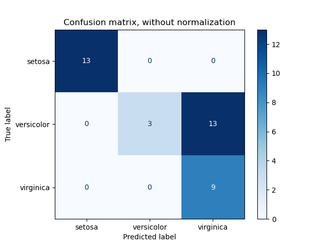
The parameter normalize allows to report ratios instead of counts. The
confusion matrix can be normalized in 3 different ways: 'pred', 'true',
and 'all' which will divide the counts by the sum of each columns, rows, or
the entire matrix, respectively.
>>> y_true = [0, 0, 0, 1, 1, 1, 1, 1]
>>> y_pred = [0, 1, 0, 1, 0, 1, 0, 1]
>>> confusion_matrix(y_true, y_pred, normalize='all')
array([[0.25 , 0.125],
       [0.25 , 0.375]])
For binary problems, we can get counts of true negatives, false positives,
false negatives and true positives as follows:
>>> y_true = [0, 0, 0, 1, 1, 1, 1, 1]
>>> y_pred = [0, 1, 0, 1, 0, 1, 0, 1]
>>> tn, fp, fn, tp = confusion_matrix(y_true, y_pred).ravel()
>>> tn, fp, fn, tp
(2, 1, 2, 3)
3.3.2.7. Classification report
The classification_report function builds a text report showing the
main classification metrics. Here is a small example with custom target_names
and inferred labels:
>>> from sklearn.metrics import classification_report
>>> y_true = [0, 1, 2, 2, 0]
>>> y_pred = [0, 0, 2, 1, 0]
>>> target_names = ['class 0', 'class 1', 'class 2']
>>> print(classification_report(y_true, y_pred, target_names=target_names))
              precision    recall  f1-score   support

     class 0       0.67      1.00      0.80         2
     class 1       0.00      0.00      0.00         1
     class 2       1.00      0.50      0.67         2

    accuracy                           0.60         5
   macro avg       0.56      0.50      0.49         5
weighted avg       0.67      0.60      0.59         5
3.3.2.8. Hamming loss
The hamming_loss computes the average Hamming loss or Hamming
distance between two sets
of samples.
If (hat{y}_{i,j}) is the predicted value for the (j)-th label of a
given sample (i), (y_{i,j}) is the corresponding true value,
(n_text{samples}) is the number of samples and (n_text{labels})
is the number of labels, then the Hamming loss (L_{Hamming}) is defined
as:
[L_{Hamming}(y, hat{y}) = frac{1}{n_text{samples} * n_text{labels}} sum_{i=0}^{n_text{samples}-1} sum_{j=0}^{n_text{labels} — 1} 1(hat{y}_{i,j} not= y_{i,j})]
where (1(x)) is the indicator function.
The equation above does not hold true in the case of multiclass classification.
Please refer to the note below for more information.
>>> from sklearn.metrics import hamming_loss
>>> y_pred = [1, 2, 3, 4]
>>> y_true = [2, 2, 3, 4]
>>> hamming_loss(y_true, y_pred)
0.25
In the multilabel case with binary label indicators:
>>> hamming_loss(np.array([[0, 1], [1, 1]]), np.zeros((2, 2)))
0.75
Note
In multiclass classification, the Hamming loss corresponds to the Hamming
distance between y_true and y_pred which is similar to the
Zero one loss function. However, while zero-one loss penalizes
prediction sets that do not strictly match true sets, the Hamming loss
penalizes individual labels. Thus the Hamming loss, upper bounded by the zero-one
loss, is always between zero and one, inclusive; and predicting a proper subset
or superset of the true labels will give a Hamming loss between
zero and one, exclusive.
3.3.2.9. Precision, recall and F-measures
Intuitively, precision is the ability
of the classifier not to label as positive a sample that is negative, and
recall is the
ability of the classifier to find all the positive samples.
The F-measure
((F_beta) and (F_1) measures) can be interpreted as a weighted
harmonic mean of the precision and recall. A
(F_beta) measure reaches its best value at 1 and its worst score at 0.
With (beta = 1), (F_beta) and
(F_1) are equivalent, and the recall and the precision are equally important.
The precision_recall_curve computes a precision-recall curve
from the ground truth label and a score given by the classifier
by varying a decision threshold.
The average_precision_score function computes the
average precision
(AP) from prediction scores. The value is between 0 and 1 and higher is better.
AP is defined as
[text{AP} = sum_n (R_n — R_{n-1}) P_n]
where (P_n) and (R_n) are the precision and recall at the
nth threshold. With random predictions, the AP is the fraction of positive
samples.
References [Manning2008] and [Everingham2010] present alternative variants of
AP that interpolate the precision-recall curve. Currently,
average_precision_score does not implement any interpolated variant.
References [Davis2006] and [Flach2015] describe why a linear interpolation of
points on the precision-recall curve provides an overly-optimistic measure of
classifier performance. This linear interpolation is used when computing area
under the curve with the trapezoidal rule in auc.
Several functions allow you to analyze the precision, recall and F-measures
score:
|
|
Compute average precision (AP) from prediction scores. |
|
|
Compute the F1 score, also known as balanced F-score or F-measure. |
|
|
Compute the F-beta score. |
|
|
Compute precision-recall pairs for different probability thresholds. |
|
|
Compute precision, recall, F-measure and support for each class. |
|
|
Compute the precision. |
|
|
Compute the recall. |
Note that the precision_recall_curve function is restricted to the
binary case. The average_precision_score function works only in
binary classification and multilabel indicator format.
The PredictionRecallDisplay.from_estimator and
PredictionRecallDisplay.from_predictions functions will plot the
precision-recall curve as follows.
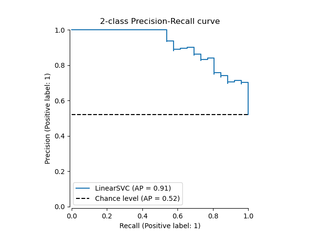
3.3.2.9.1. Binary classification
In a binary classification task, the terms ‘’positive’’ and ‘’negative’’ refer
to the classifier’s prediction, and the terms ‘’true’’ and ‘’false’’ refer to
whether that prediction corresponds to the external judgment (sometimes known
as the ‘’observation’’). Given these definitions, we can formulate the
following table:
|
Actual class (observation) |
||
|
Predicted class |
tp (true positive) |
fp (false positive) |
|
fn (false negative) |
tn (true negative) |
In this context, we can define the notions of precision, recall and F-measure:
[text{precision} = frac{tp}{tp + fp},]
[text{recall} = frac{tp}{tp + fn},]
[F_beta = (1 + beta^2) frac{text{precision} times text{recall}}{beta^2 text{precision} + text{recall}}.]
Sometimes recall is also called ‘’sensitivity’’.
Here are some small examples in binary classification:
>>> from sklearn import metrics
>>> y_pred = [0, 1, 0, 0]
>>> y_true = [0, 1, 0, 1]
>>> metrics.precision_score(y_true, y_pred)
1.0
>>> metrics.recall_score(y_true, y_pred)
0.5
>>> metrics.f1_score(y_true, y_pred)
0.66...
>>> metrics.fbeta_score(y_true, y_pred, beta=0.5)
0.83...
>>> metrics.fbeta_score(y_true, y_pred, beta=1)
0.66...
>>> metrics.fbeta_score(y_true, y_pred, beta=2)
0.55...
>>> metrics.precision_recall_fscore_support(y_true, y_pred, beta=0.5)
(array([0.66..., 1.        ]), array([1. , 0.5]), array([0.71..., 0.83...]), array([2, 2]))


>>> import numpy as np
>>> from sklearn.metrics import precision_recall_curve
>>> from sklearn.metrics import average_precision_score
>>> y_true = np.array([0, 0, 1, 1])
>>> y_scores = np.array([0.1, 0.4, 0.35, 0.8])
>>> precision, recall, threshold = precision_recall_curve(y_true, y_scores)
>>> precision
array([0.5       , 0.66..., 0.5       , 1.        , 1.        ])
>>> recall
array([1. , 1. , 0.5, 0.5, 0. ])
>>> threshold
array([0.1 , 0.35, 0.4 , 0.8 ])
>>> average_precision_score(y_true, y_scores)
0.83...
3.3.2.9.2. Multiclass and multilabel classification
In a multiclass and multilabel classification task, the notions of precision,
recall, and F-measures can be applied to each label independently.
There are a few ways to combine results across labels,
specified by the average argument to the
average_precision_score (multilabel only), f1_score,
fbeta_score, precision_recall_fscore_support,
precision_score and recall_score functions, as described
above. Note that if all labels are included, “micro”-averaging
in a multiclass setting will produce precision, recall and (F)
that are all identical to accuracy. Also note that “weighted” averaging may
produce an F-score that is not between precision and recall.
To make this more explicit, consider the following notation:
-
(y) the set of true ((sample, label)) pairs
-
(hat{y}) the set of predicted ((sample, label)) pairs
-
(L) the set of labels
-
(S) the set of samples
-
(y_s) the subset of (y) with sample (s),
i.e. (y_s := left{(s’, l) in y | s’ = sright}) -
(y_l) the subset of (y) with label (l)
-
similarly, (hat{y}_s) and (hat{y}_l) are subsets of
(hat{y}) -
(P(A, B) := frac{left| A cap B right|}{left|Bright|}) for some
sets (A) and (B) -
(R(A, B) := frac{left| A cap B right|}{left|Aright|})
(Conventions vary on handling (A = emptyset); this implementation uses
(R(A, B):=0), and similar for (P).) -
(F_beta(A, B) := left(1 + beta^2right) frac{P(A, B) times R(A, B)}{beta^2 P(A, B) + R(A, B)})
Then the metrics are defined as:
|
|
Precision |
Recall |
F_beta |
|---|---|---|---|
|
|
(P(y, hat{y})) |
(R(y, hat{y})) |
(F_beta(y, hat{y})) |
|
|
(frac{1}{left|Sright|} sum_{s in S} P(y_s, hat{y}_s)) |
(frac{1}{left|Sright|} sum_{s in S} R(y_s, hat{y}_s)) |
(frac{1}{left|Sright|} sum_{s in S} F_beta(y_s, hat{y}_s)) |
|
|
(frac{1}{left|Lright|} sum_{l in L} P(y_l, hat{y}_l)) |
(frac{1}{left|Lright|} sum_{l in L} R(y_l, hat{y}_l)) |
(frac{1}{left|Lright|} sum_{l in L} F_beta(y_l, hat{y}_l)) |
|
|
(frac{1}{sum_{l in L} left|y_lright|} sum_{l in L} left|y_lright| P(y_l, hat{y}_l)) |
(frac{1}{sum_{l in L} left|y_lright|} sum_{l in L} left|y_lright| R(y_l, hat{y}_l)) |
(frac{1}{sum_{l in L} left|y_lright|} sum_{l in L} left|y_lright| F_beta(y_l, hat{y}_l)) |
|
|
(langle P(y_l, hat{y}_l) | l in L rangle) |
(langle R(y_l, hat{y}_l) | l in L rangle) |
(langle F_beta(y_l, hat{y}_l) | l in L rangle) |
>>> from sklearn import metrics
>>> y_true = [0, 1, 2, 0, 1, 2]
>>> y_pred = [0, 2, 1, 0, 0, 1]
>>> metrics.precision_score(y_true, y_pred, average='macro')
0.22...
>>> metrics.recall_score(y_true, y_pred, average='micro')
0.33...
>>> metrics.f1_score(y_true, y_pred, average='weighted')
0.26...
>>> metrics.fbeta_score(y_true, y_pred, average='macro', beta=0.5)
0.23...
>>> metrics.precision_recall_fscore_support(y_true, y_pred, beta=0.5, average=None)
(array([0.66..., 0.        , 0.        ]), array([1., 0., 0.]), array([0.71..., 0.        , 0.        ]), array([2, 2, 2]...))
For multiclass classification with a “negative class”, it is possible to exclude some labels:
>>> metrics.recall_score(y_true, y_pred, labels=[1, 2], average='micro')
... # excluding 0, no labels were correctly recalled
0.0
Similarly, labels not present in the data sample may be accounted for in macro-averaging.
>>> metrics.precision_score(y_true, y_pred, labels=[0, 1, 2, 3], average='macro')
0.166...
3.3.2.10. Jaccard similarity coefficient score
The jaccard_score function computes the average of Jaccard similarity
coefficients, also called the
Jaccard index, between pairs of label sets.
The Jaccard similarity coefficient with a ground truth label set (y) and
predicted label set (hat{y}), is defined as
[J(y, hat{y}) = frac{|y cap hat{y}|}{|y cup hat{y}|}.]
The jaccard_score (like precision_recall_fscore_support) applies
natively to binary targets. By computing it set-wise it can be extended to apply
to multilabel and multiclass through the use of average (see
above).
In the binary case:
>>> import numpy as np
>>> from sklearn.metrics import jaccard_score
>>> y_true = np.array([[0, 1, 1],
...                    [1, 1, 0]])
>>> y_pred = np.array([[1, 1, 1],
...                    [1, 0, 0]])
>>> jaccard_score(y_true[0], y_pred[0])
0.6666...
In the 2D comparison case (e.g. image similarity):
>>> jaccard_score(y_true, y_pred, average="micro")
0.6
In the multilabel case with binary label indicators:
>>> jaccard_score(y_true, y_pred, average='samples')
0.5833...
>>> jaccard_score(y_true, y_pred, average='macro')
0.6666...
>>> jaccard_score(y_true, y_pred, average=None)
array([0.5, 0.5, 1. ])
Multiclass problems are binarized and treated like the corresponding
multilabel problem:
>>> y_pred = [0, 2, 1, 2]
>>> y_true = [0, 1, 2, 2]
>>> jaccard_score(y_true, y_pred, average=None)
array([1. , 0. , 0.33...])
>>> jaccard_score(y_true, y_pred, average='macro')
0.44...
>>> jaccard_score(y_true, y_pred, average='micro')
0.33...
3.3.2.11. Hinge loss
The hinge_loss function computes the average distance between
the model and the data using
hinge loss, a one-sided metric
that considers only prediction errors. (Hinge
loss is used in maximal margin classifiers such as support vector machines.)
If the true label (y_i) of a binary classification task is encoded as
(y_i=left{-1, +1right}) for every sample (i); and (w_i)
is the corresponding predicted decision (an array of shape (n_samples,) as
output by the decision_function method), then the hinge loss is defined as:
[L_text{Hinge}(y, w) = frac{1}{n_text{samples}} sum_{i=0}^{n_text{samples}-1} maxleft{1 — w_i y_i, 0right}]
If there are more than two labels, hinge_loss uses a multiclass variant
due to Crammer & Singer.
Here is
the paper describing it.
In this case the predicted decision is an array of shape (n_samples,
n_labels). If (w_{i, y_i}) is the predicted decision for the true label
(y_i) of the (i)-th sample; and
(hat{w}_{i, y_i} = maxleft{w_{i, y_j}~|~y_j ne y_i right})
is the maximum of the
predicted decisions for all the other labels, then the multi-class hinge loss
is defined by:
[L_text{Hinge}(y, w) = frac{1}{n_text{samples}}
sum_{i=0}^{n_text{samples}-1} maxleft{1 + hat{w}_{i, y_i}
— w_{i, y_i}, 0right}]
Here is a small example demonstrating the use of the hinge_loss function
with a svm classifier in a binary class problem:
>>> from sklearn import svm
>>> from sklearn.metrics import hinge_loss
>>> X = [[0], [1]]
>>> y = [-1, 1]
>>> est = svm.LinearSVC(random_state=0)
>>> est.fit(X, y)
LinearSVC(random_state=0)
>>> pred_decision = est.decision_function([[-2], [3], [0.5]])
>>> pred_decision
array([-2.18...,  2.36...,  0.09...])
>>> hinge_loss([-1, 1, 1], pred_decision)
0.3...
Here is an example demonstrating the use of the hinge_loss function
with a svm classifier in a multiclass problem:
>>> X = np.array([[0], [1], [2], [3]])
>>> Y = np.array([0, 1, 2, 3])
>>> labels = np.array([0, 1, 2, 3])
>>> est = svm.LinearSVC()
>>> est.fit(X, Y)
LinearSVC()
>>> pred_decision = est.decision_function([[-1], [2], [3]])
>>> y_true = [0, 2, 3]
>>> hinge_loss(y_true, pred_decision, labels=labels)
0.56...
3.3.2.12. Log loss
Log loss, also called logistic regression loss or
cross-entropy loss, is defined on probability estimates. It is
commonly used in (multinomial) logistic regression and neural networks, as well
as in some variants of expectation-maximization, and can be used to evaluate the
probability outputs (predict_proba) of a classifier instead of its
discrete predictions.
For binary classification with a true label (y in {0,1})
and a probability estimate (p = operatorname{Pr}(y = 1)),
the log loss per sample is the negative log-likelihood
of the classifier given the true label:
[L_{log}(y, p) = -log operatorname{Pr}(y|p) = -(y log (p) + (1 — y) log (1 — p))]
This extends to the multiclass case as follows.
Let the true labels for a set of samples
be encoded as a 1-of-K binary indicator matrix (Y),
i.e., (y_{i,k} = 1) if sample (i) has label (k)
taken from a set of (K) labels.
Let (P) be a matrix of probability estimates,
with (p_{i,k} = operatorname{Pr}(y_{i,k} = 1)).
Then the log loss of the whole set is
[L_{log}(Y, P) = -log operatorname{Pr}(Y|P) = — frac{1}{N} sum_{i=0}^{N-1} sum_{k=0}^{K-1} y_{i,k} log p_{i,k}]
To see how this generalizes the binary log loss given above,
note that in the binary case,
(p_{i,0} = 1 — p_{i,1}) and (y_{i,0} = 1 — y_{i,1}),
so expanding the inner sum over (y_{i,k} in {0,1})
gives the binary log loss.
The log_loss function computes log loss given a list of ground-truth
labels and a probability matrix, as returned by an estimator’s predict_proba
method.
>>> from sklearn.metrics import log_loss
>>> y_true = [0, 0, 1, 1]
>>> y_pred = [[.9, .1], [.8, .2], [.3, .7], [.01, .99]]
>>> log_loss(y_true, y_pred)
0.1738...
The first [.9, .1] in y_pred denotes 90% probability that the first
sample has label 0. The log loss is non-negative.
3.3.2.13. Matthews correlation coefficient
The matthews_corrcoef function computes the
Matthew’s correlation coefficient (MCC)
for binary classes. Quoting Wikipedia:
“The Matthews correlation coefficient is used in machine learning as a
measure of the quality of binary (two-class) classifications. It takes
into account true and false positives and negatives and is generally
regarded as a balanced measure which can be used even if the classes are
of very different sizes. The MCC is in essence a correlation coefficient
value between -1 and +1. A coefficient of +1 represents a perfect
prediction, 0 an average random prediction and -1 an inverse prediction.
The statistic is also known as the phi coefficient.”
In the binary (two-class) case, (tp), (tn), (fp) and
(fn) are respectively the number of true positives, true negatives, false
positives and false negatives, the MCC is defined as
[MCC = frac{tp times tn — fp times fn}{sqrt{(tp + fp)(tp + fn)(tn + fp)(tn + fn)}}.]
In the multiclass case, the Matthews correlation coefficient can be defined in terms of a
confusion_matrix (C) for (K) classes. To simplify the
definition consider the following intermediate variables:
-
(t_k=sum_{i}^{K} C_{ik}) the number of times class (k) truly occurred,
-
(p_k=sum_{i}^{K} C_{ki}) the number of times class (k) was predicted,
-
(c=sum_{k}^{K} C_{kk}) the total number of samples correctly predicted,
-
(s=sum_{i}^{K} sum_{j}^{K} C_{ij}) the total number of samples.
Then the multiclass MCC is defined as:
[MCC = frac{
c times s — sum_{k}^{K} p_k times t_k
}{sqrt{
(s^2 — sum_{k}^{K} p_k^2) times
(s^2 — sum_{k}^{K} t_k^2)
}}]
When there are more than two labels, the value of the MCC will no longer range
between -1 and +1. Instead the minimum value will be somewhere between -1 and 0
depending on the number and distribution of ground true labels. The maximum
value is always +1.
Here is a small example illustrating the usage of the matthews_corrcoef
function:
>>> from sklearn.metrics import matthews_corrcoef
>>> y_true = [+1, +1, +1, -1]
>>> y_pred = [+1, -1, +1, +1]
>>> matthews_corrcoef(y_true, y_pred)
-0.33...
3.3.2.14. Multi-label confusion matrix
The multilabel_confusion_matrix function computes class-wise (default)
or sample-wise (samplewise=True) multilabel confusion matrix to evaluate
the accuracy of a classification. multilabel_confusion_matrix also treats
multiclass data as if it were multilabel, as this is a transformation commonly
applied to evaluate multiclass problems with binary classification metrics
(such as precision, recall, etc.).
When calculating class-wise multilabel confusion matrix (C), the
count of true negatives for class (i) is (C_{i,0,0}), false
negatives is (C_{i,1,0}), true positives is (C_{i,1,1})
and false positives is (C_{i,0,1}).
Here is an example demonstrating the use of the
multilabel_confusion_matrix function with
multilabel indicator matrix input:
>>> import numpy as np
>>> from sklearn.metrics import multilabel_confusion_matrix
>>> y_true = np.array([[1, 0, 1],
...                    [0, 1, 0]])
>>> y_pred = np.array([[1, 0, 0],
...                    [0, 1, 1]])
>>> multilabel_confusion_matrix(y_true, y_pred)
array([[[1, 0],
        [0, 1]],

       [[1, 0],
        [0, 1]],

       [[0, 1],
        [1, 0]]])
Or a confusion matrix can be constructed for each sample’s labels:
>>> multilabel_confusion_matrix(y_true, y_pred, samplewise=True)
array([[[1, 0],
        [1, 1]],

       [[1, 1],
        [0, 1]]])
Here is an example demonstrating the use of the
multilabel_confusion_matrix function with
multiclass input:
>>> y_true = ["cat", "ant", "cat", "cat", "ant", "bird"]
>>> y_pred = ["ant", "ant", "cat", "cat", "ant", "cat"]
>>> multilabel_confusion_matrix(y_true, y_pred,
...                             labels=["ant", "bird", "cat"])
array([[[3, 1],
        [0, 2]],

       [[5, 0],
        [1, 0]],

       [[2, 1],
        [1, 2]]])
Here are some examples demonstrating the use of the
multilabel_confusion_matrix function to calculate recall
(or sensitivity), specificity, fall out and miss rate for each class in a
problem with multilabel indicator matrix input.
Calculating
recall
(also called the true positive rate or the sensitivity) for each class:
>>> y_true = np.array([[0, 0, 1],
...                    [0, 1, 0],
...                    [1, 1, 0]])
>>> y_pred = np.array([[0, 1, 0],
...                    [0, 0, 1],
...                    [1, 1, 0]])
>>> mcm = multilabel_confusion_matrix(y_true, y_pred)
>>> tn = mcm[:, 0, 0]
>>> tp = mcm[:, 1, 1]
>>> fn = mcm[:, 1, 0]
>>> fp = mcm[:, 0, 1]
>>> tp / (tp + fn)
array([1. , 0.5, 0. ])
Calculating
specificity
(also called the true negative rate) for each class:
>>> tn / (tn + fp)
array([1. , 0. , 0.5])
Calculating fall out
(also called the false positive rate) for each class:
>>> fp / (fp + tn)
array([0. , 1. , 0.5])
Calculating miss rate
(also called the false negative rate) for each class:
>>> fn / (fn + tp)
array([0. , 0.5, 1. ])
3.3.2.15. Receiver operating characteristic (ROC)
The function roc_curve computes the
receiver operating characteristic curve, or ROC curve.
Quoting Wikipedia :
“A receiver operating characteristic (ROC), or simply ROC curve, is a
graphical plot which illustrates the performance of a binary classifier
system as its discrimination threshold is varied. It is created by plotting
the fraction of true positives out of the positives (TPR = true positive
rate) vs. the fraction of false positives out of the negatives (FPR = false
positive rate), at various threshold settings. TPR is also known as
sensitivity, and FPR is one minus the specificity or true negative rate.”
This function requires the true binary value and the target scores, which can
either be probability estimates of the positive class, confidence values, or
binary decisions. Here is a small example of how to use the roc_curve
function:
>>> import numpy as np
>>> from sklearn.metrics import roc_curve
>>> y = np.array([1, 1, 2, 2])
>>> scores = np.array([0.1, 0.4, 0.35, 0.8])
>>> fpr, tpr, thresholds = roc_curve(y, scores, pos_label=2)
>>> fpr
array([0. , 0. , 0.5, 0.5, 1. ])
>>> tpr
array([0. , 0.5, 0.5, 1. , 1. ])
>>> thresholds
array([1.8 , 0.8 , 0.4 , 0.35, 0.1 ])
Compared to metrics such as the subset accuracy, the Hamming loss, or the
F1 score, ROC doesn’t require optimizing a threshold for each label.
The roc_auc_score function, denoted by ROC-AUC or AUROC, computes the
area under the ROC curve. By doing so, the curve information is summarized in
one number.
The following figure shows the ROC curve and ROC-AUC score for a classifier
aimed to distinguish the virginica flower from the rest of the species in the
Iris plants dataset:
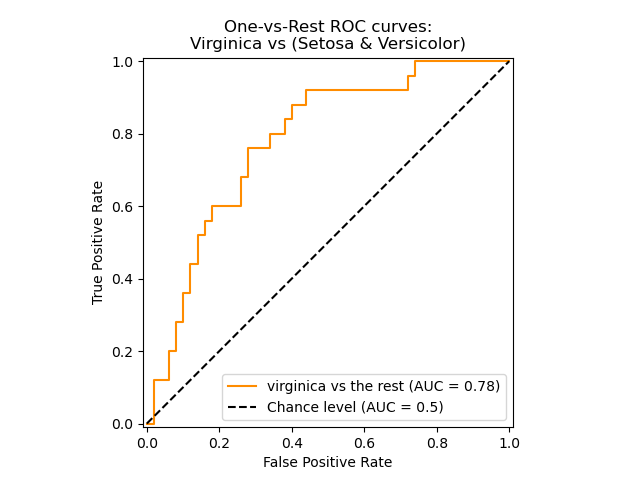
For more information see the Wikipedia article on AUC.
3.3.2.15.1. Binary case
In the binary case, you can either provide the probability estimates, using
the classifier.predict_proba() method, or the non-thresholded decision values
given by the classifier.decision_function() method. In the case of providing
the probability estimates, the probability of the class with the
“greater label” should be provided. The “greater label” corresponds to
classifier.classes_[1] and thus classifier.predict_proba(X)[:, 1].
Therefore, the y_score parameter is of size (n_samples,).
>>> from sklearn.datasets import load_breast_cancer
>>> from sklearn.linear_model import LogisticRegression
>>> from sklearn.metrics import roc_auc_score
>>> X, y = load_breast_cancer(return_X_y=True)
>>> clf = LogisticRegression(solver="liblinear").fit(X, y)
>>> clf.classes_
array([0, 1])
We can use the probability estimates corresponding to clf.classes_[1].
>>> y_score = clf.predict_proba(X)[:, 1]
>>> roc_auc_score(y, y_score)
0.99...
Otherwise, we can use the non-thresholded decision values
>>> roc_auc_score(y, clf.decision_function(X))
0.99...
3.3.2.15.2. Multi-class case
The roc_auc_score function can also be used in multi-class
classification. Two averaging strategies are currently supported: the
one-vs-one algorithm computes the average of the pairwise ROC AUC scores, and
the one-vs-rest algorithm computes the average of the ROC AUC scores for each
class against all other classes. In both cases, the predicted labels are
provided in an array with values from 0 to n_classes, and the scores
correspond to the probability estimates that a sample belongs to a particular
class. The OvO and OvR algorithms support weighting uniformly
(average='macro') and by prevalence (average='weighted').
One-vs-one Algorithm: Computes the average AUC of all possible pairwise
combinations of classes. [HT2001] defines a multiclass AUC metric weighted
uniformly:
[frac{1}{c(c-1)}sum_{j=1}^{c}sum_{k > j}^c (text{AUC}(j | k) +
text{AUC}(k | j))]
where (c) is the number of classes and (text{AUC}(j | k)) is the
AUC with class (j) as the positive class and class (k) as the
negative class. In general,
(text{AUC}(j | k) neq text{AUC}(k | j))) in the multiclass
case. This algorithm is used by setting the keyword argument multiclass
to 'ovo' and average to 'macro'.
The [HT2001] multiclass AUC metric can be extended to be weighted by the
prevalence:
[frac{1}{c(c-1)}sum_{j=1}^{c}sum_{k > j}^c p(j cup k)(
text{AUC}(j | k) + text{AUC}(k | j))]
where (c) is the number of classes. This algorithm is used by setting
the keyword argument multiclass to 'ovo' and average to
'weighted'. The 'weighted' option returns a prevalence-weighted average
as described in [FC2009].
One-vs-rest Algorithm: Computes the AUC of each class against the rest
[PD2000]. The algorithm is functionally the same as the multilabel case. To
enable this algorithm set the keyword argument multiclass to 'ovr'.
Additionally to 'macro' [F2006] and 'weighted' [F2001] averaging, OvR
supports 'micro' averaging.
In applications where a high false positive rate is not tolerable the parameter
max_fpr of roc_auc_score can be used to summarize the ROC curve up
to the given limit.
The following figure shows the micro-averaged ROC curve and its corresponding
ROC-AUC score for a classifier aimed to distinguish the the different species in
the Iris plants dataset:
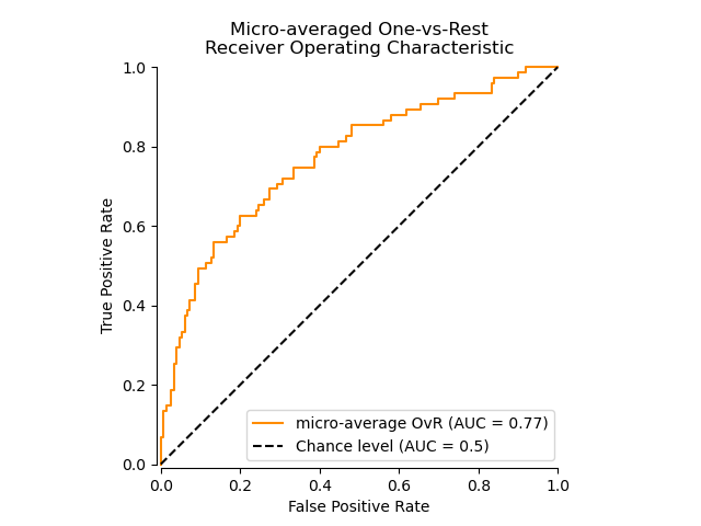
3.3.2.15.3. Multi-label case
In multi-label classification, the roc_auc_score function is
extended by averaging over the labels as above. In this case,
you should provide a y_score of shape (n_samples, n_classes). Thus, when
using the probability estimates, one needs to select the probability of the
class with the greater label for each output.
>>> from sklearn.datasets import make_multilabel_classification
>>> from sklearn.multioutput import MultiOutputClassifier
>>> X, y = make_multilabel_classification(random_state=0)
>>> inner_clf = LogisticRegression(solver="liblinear", random_state=0)
>>> clf = MultiOutputClassifier(inner_clf).fit(X, y)
>>> y_score = np.transpose([y_pred[:, 1] for y_pred in clf.predict_proba(X)])
>>> roc_auc_score(y, y_score, average=None)
array([0.82..., 0.86..., 0.94..., 0.85... , 0.94...])
And the decision values do not require such processing.
>>> from sklearn.linear_model import RidgeClassifierCV
>>> clf = RidgeClassifierCV().fit(X, y)
>>> y_score = clf.decision_function(X)
>>> roc_auc_score(y, y_score, average=None)
array([0.81..., 0.84... , 0.93..., 0.87..., 0.94...])
3.3.2.16. Detection error tradeoff (DET)
The function det_curve computes the
detection error tradeoff curve (DET) curve [WikipediaDET2017].
Quoting Wikipedia:
“A detection error tradeoff (DET) graph is a graphical plot of error rates
for binary classification systems, plotting false reject rate vs. false
accept rate. The x- and y-axes are scaled non-linearly by their standard
normal deviates (or just by logarithmic transformation), yielding tradeoff
curves that are more linear than ROC curves, and use most of the image area
to highlight the differences of importance in the critical operating region.”
DET curves are a variation of receiver operating characteristic (ROC) curves
where False Negative Rate is plotted on the y-axis instead of True Positive
Rate.
DET curves are commonly plotted in normal deviate scale by transformation with
(phi^{-1}) (with (phi) being the cumulative distribution
function).
The resulting performance curves explicitly visualize the tradeoff of error
types for given classification algorithms.
See [Martin1997] for examples and further motivation.
This figure compares the ROC and DET curves of two example classifiers on the
same classification task:
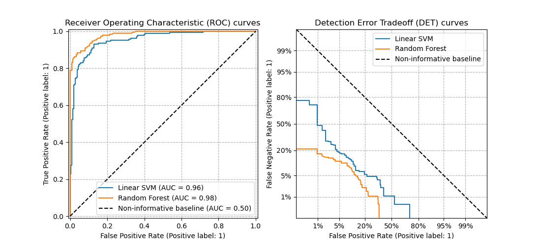
Properties:
-
DET curves form a linear curve in normal deviate scale if the detection
scores are normally (or close-to normally) distributed.
It was shown by [Navratil2007] that the reverse is not necessarily true and
even more general distributions are able to produce linear DET curves. -
The normal deviate scale transformation spreads out the points such that a
comparatively larger space of plot is occupied.
Therefore curves with similar classification performance might be easier to
distinguish on a DET plot. -
With False Negative Rate being “inverse” to True Positive Rate the point
of perfection for DET curves is the origin (in contrast to the top left
corner for ROC curves).
Applications and limitations:
DET curves are intuitive to read and hence allow quick visual assessment of a
classifier’s performance.
Additionally DET curves can be consulted for threshold analysis and operating
point selection.
This is particularly helpful if a comparison of error types is required.
On the other hand DET curves do not provide their metric as a single number.
Therefore for either automated evaluation or comparison to other
classification tasks metrics like the derived area under ROC curve might be
better suited.
3.3.2.17. Zero one loss
The zero_one_loss function computes the sum or the average of the 0-1
classification loss ((L_{0-1})) over (n_{text{samples}}). By
default, the function normalizes over the sample. To get the sum of the
(L_{0-1}), set normalize to False.
In multilabel classification, the zero_one_loss scores a subset as
one if its labels strictly match the predictions, and as a zero if there
are any errors. By default, the function returns the percentage of imperfectly
predicted subsets. To get the count of such subsets instead, set
normalize to False
If (hat{y}_i) is the predicted value of
the (i)-th sample and (y_i) is the corresponding true value,
then the 0-1 loss (L_{0-1}) is defined as:
[L_{0-1}(y, hat{y}) = frac{1}{n_text{samples}} sum_{i=0}^{n_text{samples}-1} 1(hat{y}_i not= y_i)]
where (1(x)) is the indicator function. The zero one
loss can also be computed as (zero-one loss = 1 — accuracy).
>>> from sklearn.metrics import zero_one_loss
>>> y_pred = [1, 2, 3, 4]
>>> y_true = [2, 2, 3, 4]
>>> zero_one_loss(y_true, y_pred)
0.25
>>> zero_one_loss(y_true, y_pred, normalize=False)
1
In the multilabel case with binary label indicators, where the first label
set [0,1] has an error:
>>> zero_one_loss(np.array([[0, 1], [1, 1]]), np.ones((2, 2)))
0.5

>>> zero_one_loss(np.array([[0, 1], [1, 1]]), np.ones((2, 2)),  normalize=False)
1
3.3.2.18. Brier score loss
The brier_score_loss function computes the
Brier score
for binary classes [Brier1950]. Quoting Wikipedia:
“The Brier score is a proper score function that measures the accuracy of
probabilistic predictions. It is applicable to tasks in which predictions
must assign probabilities to a set of mutually exclusive discrete outcomes.”
This function returns the mean squared error of the actual outcome
(y in {0,1}) and the predicted probability estimate
(p = operatorname{Pr}(y = 1)) (predict_proba) as outputted by:
[BS = frac{1}{n_{text{samples}}} sum_{i=0}^{n_{text{samples}} — 1}(y_i — p_i)^2]
The Brier score loss is also between 0 to 1 and the lower the value (the mean
square difference is smaller), the more accurate the prediction is.
Here is a small example of usage of this function:
>>> import numpy as np
>>> from sklearn.metrics import brier_score_loss
>>> y_true = np.array([0, 1, 1, 0])
>>> y_true_categorical = np.array(["spam", "ham", "ham", "spam"])
>>> y_prob = np.array([0.1, 0.9, 0.8, 0.4])
>>> y_pred = np.array([0, 1, 1, 0])
>>> brier_score_loss(y_true, y_prob)
0.055
>>> brier_score_loss(y_true, 1 - y_prob, pos_label=0)
0.055
>>> brier_score_loss(y_true_categorical, y_prob, pos_label="ham")
0.055
>>> brier_score_loss(y_true, y_prob > 0.5)
0.0
The Brier score can be used to assess how well a classifier is calibrated.
However, a lower Brier score loss does not always mean a better calibration.
This is because, by analogy with the bias-variance decomposition of the mean
squared error, the Brier score loss can be decomposed as the sum of calibration
loss and refinement loss [Bella2012]. Calibration loss is defined as the mean
squared deviation from empirical probabilities derived from the slope of ROC
segments. Refinement loss can be defined as the expected optimal loss as
measured by the area under the optimal cost curve. Refinement loss can change
independently from calibration loss, thus a lower Brier score loss does not
necessarily mean a better calibrated model. “Only when refinement loss remains
the same does a lower Brier score loss always mean better calibration”
[Bella2012], [Flach2008].
3.3.2.19. Class likelihood ratios
The class_likelihood_ratios function computes the positive and negative
likelihood ratios
(LR_pm) for binary classes, which can be interpreted as the ratio of
post-test to pre-test odds as explained below. As a consequence, this metric is
invariant w.r.t. the class prevalence (the number of samples in the positive
class divided by the total number of samples) and can be extrapolated between
populations regardless of any possible class imbalance.
The (LR_pm) metrics are therefore very useful in settings where the data
available to learn and evaluate a classifier is a study population with nearly
balanced classes, such as a case-control study, while the target application,
i.e. the general population, has very low prevalence.
The positive likelihood ratio (LR_+) is the probability of a classifier to
correctly predict that a sample belongs to the positive class divided by the
probability of predicting the positive class for a sample belonging to the
negative class:
[LR_+ = frac{text{PR}(P+|T+)}{text{PR}(P+|T-)}.]
The notation here refers to predicted ((P)) or true ((T)) label and
the sign (+) and (-) refer to the positive and negative class,
respectively, e.g. (P+) stands for “predicted positive”.
Analogously, the negative likelihood ratio (LR_-) is the probability of a
sample of the positive class being classified as belonging to the negative class
divided by the probability of a sample of the negative class being correctly
classified:
[LR_- = frac{text{PR}(P-|T+)}{text{PR}(P-|T-)}.]
For classifiers above chance (LR_+) above 1 higher is better, while
(LR_-) ranges from 0 to 1 and lower is better.
Values of (LR_pmapprox 1) correspond to chance level.
Notice that probabilities differ from counts, for instance
(operatorname{PR}(P+|T+)) is not equal to the number of true positive
counts tp (see the wikipedia page for
the actual formulas).
Interpretation across varying prevalence:
Both class likelihood ratios are interpretable in terms of an odds ratio
(pre-test and post-tests):
[text{post-test odds} = text{Likelihood ratio} times text{pre-test odds}.]
Odds are in general related to probabilities via
[text{odds} = frac{text{probability}}{1 — text{probability}},]
or equivalently
[text{probability} = frac{text{odds}}{1 + text{odds}}.]
On a given population, the pre-test probability is given by the prevalence. By
converting odds to probabilities, the likelihood ratios can be translated into a
probability of truly belonging to either class before and after a classifier
prediction:
[text{post-test odds} = text{Likelihood ratio} times
frac{text{pre-test probability}}{1 — text{pre-test probability}},]
[text{post-test probability} = frac{text{post-test odds}}{1 + text{post-test odds}}.]
Mathematical divergences:
The positive likelihood ratio is undefined when (fp = 0), which can be
interpreted as the classifier perfectly identifying positive cases. If (fp
= 0) and additionally (tp = 0), this leads to a zero/zero division. This
happens, for instance, when using a DummyClassifier that always predicts the
negative class and therefore the interpretation as a perfect classifier is lost.
The negative likelihood ratio is undefined when (tn = 0). Such divergence
is invalid, as (LR_- > 1) would indicate an increase in the odds of a
sample belonging to the positive class after being classified as negative, as if
the act of classifying caused the positive condition. This includes the case of
a DummyClassifier that always predicts the positive class (i.e. when
(tn=fn=0)).
Both class likelihood ratios are undefined when (tp=fn=0), which means
that no samples of the positive class were present in the testing set. This can
also happen when cross-validating highly imbalanced data.
In all the previous cases the class_likelihood_ratios function raises by
default an appropriate warning message and returns nan to avoid pollution when
averaging over cross-validation folds.
For a worked-out demonstration of the class_likelihood_ratios function,
see the example below.
3.3.3. Multilabel ranking metrics
In multilabel learning, each sample can have any number of ground truth labels
associated with it. The goal is to give high scores and better rank to
the ground truth labels.
3.3.3.1. Coverage error
The coverage_error function computes the average number of labels that
have to be included in the final prediction such that all true labels
are predicted. This is useful if you want to know how many top-scored-labels
you have to predict in average without missing any true one. The best value
of this metrics is thus the average number of true labels.
Note
Our implementation’s score is 1 greater than the one given in Tsoumakas
et al., 2010. This extends it to handle the degenerate case in which an
instance has 0 true labels.
Formally, given a binary indicator matrix of the ground truth labels
(y in left{0, 1right}^{n_text{samples} times n_text{labels}}) and the
score associated with each label
(hat{f} in mathbb{R}^{n_text{samples} times n_text{labels}}),
the coverage is defined as
[coverage(y, hat{f}) = frac{1}{n_{text{samples}}}
sum_{i=0}^{n_{text{samples}} — 1} max_{j:y_{ij} = 1} text{rank}_{ij}]
with (text{rank}_{ij} = left|left{k: hat{f}_{ik} geq hat{f}_{ij} right}right|).
Given the rank definition, ties in y_scores are broken by giving the
maximal rank that would have been assigned to all tied values.
Here is a small example of usage of this function:
>>> import numpy as np
>>> from sklearn.metrics import coverage_error
>>> y_true = np.array([[1, 0, 0], [0, 0, 1]])
>>> y_score = np.array([[0.75, 0.5, 1], [1, 0.2, 0.1]])
>>> coverage_error(y_true, y_score)
2.5
3.3.3.2. Label ranking average precision
The label_ranking_average_precision_score function
implements label ranking average precision (LRAP). This metric is linked to
the average_precision_score function, but is based on the notion of
label ranking instead of precision and recall.
Label ranking average precision (LRAP) averages over the samples the answer to
the following question: for each ground truth label, what fraction of
higher-ranked labels were true labels? This performance measure will be higher
if you are able to give better rank to the labels associated with each sample.
The obtained score is always strictly greater than 0, and the best value is 1.
If there is exactly one relevant label per sample, label ranking average
precision is equivalent to the mean
reciprocal rank.
Formally, given a binary indicator matrix of the ground truth labels
(y in left{0, 1right}^{n_text{samples} times n_text{labels}})
and the score associated with each label
(hat{f} in mathbb{R}^{n_text{samples} times n_text{labels}}),
the average precision is defined as
[LRAP(y, hat{f}) = frac{1}{n_{text{samples}}}
sum_{i=0}^{n_{text{samples}} — 1} frac{1}{||y_i||_0}
sum_{j:y_{ij} = 1} frac{|mathcal{L}_{ij}|}{text{rank}_{ij}}]
where
(mathcal{L}_{ij} = left{k: y_{ik} = 1, hat{f}_{ik} geq hat{f}_{ij} right}),
(text{rank}_{ij} = left|left{k: hat{f}_{ik} geq hat{f}_{ij} right}right|),
(|cdot|) computes the cardinality of the set (i.e., the number of
elements in the set), and (||cdot||_0) is the (ell_0) “norm”
(which computes the number of nonzero elements in a vector).
Here is a small example of usage of this function:
>>> import numpy as np
>>> from sklearn.metrics import label_ranking_average_precision_score
>>> y_true = np.array([[1, 0, 0], [0, 0, 1]])
>>> y_score = np.array([[0.75, 0.5, 1], [1, 0.2, 0.1]])
>>> label_ranking_average_precision_score(y_true, y_score)
0.416...
3.3.3.3. Ranking loss
The label_ranking_loss function computes the ranking loss which
averages over the samples the number of label pairs that are incorrectly
ordered, i.e. true labels have a lower score than false labels, weighted by
the inverse of the number of ordered pairs of false and true labels.
The lowest achievable ranking loss is zero.
Formally, given a binary indicator matrix of the ground truth labels
(y in left{0, 1right}^{n_text{samples} times n_text{labels}}) and the
score associated with each label
(hat{f} in mathbb{R}^{n_text{samples} times n_text{labels}}),
the ranking loss is defined as
[ranking_loss(y, hat{f}) = frac{1}{n_{text{samples}}}
sum_{i=0}^{n_{text{samples}} — 1} frac{1}{||y_i||_0(n_text{labels} — ||y_i||_0)}
left|left{(k, l): hat{f}_{ik} leq hat{f}_{il}, y_{ik} = 1, y_{il} = 0 right}right|]
where (|cdot|) computes the cardinality of the set (i.e., the number of
elements in the set) and (||cdot||_0) is the (ell_0) “norm”
(which computes the number of nonzero elements in a vector).
Here is a small example of usage of this function:
>>> import numpy as np
>>> from sklearn.metrics import label_ranking_loss
>>> y_true = np.array([[1, 0, 0], [0, 0, 1]])
>>> y_score = np.array([[0.75, 0.5, 1], [1, 0.2, 0.1]])
>>> label_ranking_loss(y_true, y_score)
0.75...
>>> # With the following prediction, we have perfect and minimal loss
>>> y_score = np.array([[1.0, 0.1, 0.2], [0.1, 0.2, 0.9]])
>>> label_ranking_loss(y_true, y_score)
0.0
3.3.3.4. Normalized Discounted Cumulative Gain
Discounted Cumulative Gain (DCG) and Normalized Discounted Cumulative Gain
(NDCG) are ranking metrics implemented in dcg_score
and ndcg_score ; they compare a predicted order to
ground-truth scores, such as the relevance of answers to a query.
From the Wikipedia page for Discounted Cumulative Gain:
“Discounted cumulative gain (DCG) is a measure of ranking quality. In
information retrieval, it is often used to measure effectiveness of web search
engine algorithms or related applications. Using a graded relevance scale of
documents in a search-engine result set, DCG measures the usefulness, or gain,
of a document based on its position in the result list. The gain is accumulated
from the top of the result list to the bottom, with the gain of each result
discounted at lower ranks”
DCG orders the true targets (e.g. relevance of query answers) in the predicted
order, then multiplies them by a logarithmic decay and sums the result. The sum
can be truncated after the first (K) results, in which case we call it
DCG@K.
NDCG, or NDCG@K is DCG divided by the DCG obtained by a perfect prediction, so
that it is always between 0 and 1. Usually, NDCG is preferred to DCG.
Compared with the ranking loss, NDCG can take into account relevance scores,
rather than a ground-truth ranking. So if the ground-truth consists only of an
ordering, the ranking loss should be preferred; if the ground-truth consists of
actual usefulness scores (e.g. 0 for irrelevant, 1 for relevant, 2 for very
relevant), NDCG can be used.
For one sample, given the vector of continuous ground-truth values for each
target (y in mathbb{R}^{M}), where (M) is the number of outputs, and
the prediction (hat{y}), which induces the ranking function (f), the
DCG score is
[sum_{r=1}^{min(K, M)}frac{y_{f(r)}}{log(1 + r)}]
and the NDCG score is the DCG score divided by the DCG score obtained for
(y).
3.3.4. Regression metrics
The sklearn.metrics module implements several loss, score, and utility
functions to measure regression performance. Some of those have been enhanced
to handle the multioutput case: mean_squared_error,
mean_absolute_error, r2_score,
explained_variance_score, mean_pinball_loss, d2_pinball_score
and d2_absolute_error_score.
These functions have a multioutput keyword argument which specifies the
way the scores or losses for each individual target should be averaged. The
default is 'uniform_average', which specifies a uniformly weighted mean
over outputs. If an ndarray of shape (n_outputs,) is passed, then its
entries are interpreted as weights and an according weighted average is
returned. If multioutput is 'raw_values', then all unaltered
individual scores or losses will be returned in an array of shape
(n_outputs,).
The r2_score and explained_variance_score accept an additional
value 'variance_weighted' for the multioutput parameter. This option
leads to a weighting of each individual score by the variance of the
corresponding target variable. This setting quantifies the globally captured
unscaled variance. If the target variables are of different scale, then this
score puts more importance on explaining the higher variance variables.
multioutput='variance_weighted' is the default value for r2_score
for backward compatibility. This will be changed to uniform_average in the
future.
3.3.4.1. R² score, the coefficient of determination
The r2_score function computes the coefficient of
determination,
usually denoted as (R^2).
It represents the proportion of variance (of y) that has been explained by the
independent variables in the model. It provides an indication of goodness of
fit and therefore a measure of how well unseen samples are likely to be
predicted by the model, through the proportion of explained variance.
As such variance is dataset dependent, (R^2) may not be meaningfully comparable
across different datasets. Best possible score is 1.0 and it can be negative
(because the model can be arbitrarily worse). A constant model that always
predicts the expected (average) value of y, disregarding the input features,
would get an (R^2) score of 0.0.
Note: when the prediction residuals have zero mean, the (R^2) score and
the Explained variance score are identical.
If (hat{y}_i) is the predicted value of the (i)-th sample
and (y_i) is the corresponding true value for total (n) samples,
the estimated (R^2) is defined as:
[R^2(y, hat{y}) = 1 — frac{sum_{i=1}^{n} (y_i — hat{y}_i)^2}{sum_{i=1}^{n} (y_i — bar{y})^2}]
where (bar{y} = frac{1}{n} sum_{i=1}^{n} y_i) and (sum_{i=1}^{n} (y_i — hat{y}_i)^2 = sum_{i=1}^{n} epsilon_i^2).
Note that r2_score calculates unadjusted (R^2) without correcting for
bias in sample variance of y.
In the particular case where the true target is constant, the (R^2) score is
not finite: it is either NaN (perfect predictions) or -Inf (imperfect
predictions). Such non-finite scores may prevent correct model optimization
such as grid-search cross-validation to be performed correctly. For this reason
the default behaviour of r2_score is to replace them with 1.0 (perfect
predictions) or 0.0 (imperfect predictions). If force_finite
is set to False, this score falls back on the original (R^2) definition.
Here is a small example of usage of the r2_score function:
>>> from sklearn.metrics import r2_score
>>> y_true = [3, -0.5, 2, 7]
>>> y_pred = [2.5, 0.0, 2, 8]
>>> r2_score(y_true, y_pred)
0.948...
>>> y_true = [[0.5, 1], [-1, 1], [7, -6]]
>>> y_pred = [[0, 2], [-1, 2], [8, -5]]
>>> r2_score(y_true, y_pred, multioutput='variance_weighted')
0.938...
>>> y_true = [[0.5, 1], [-1, 1], [7, -6]]
>>> y_pred = [[0, 2], [-1, 2], [8, -5]]
>>> r2_score(y_true, y_pred, multioutput='uniform_average')
0.936...
>>> r2_score(y_true, y_pred, multioutput='raw_values')
array([0.965..., 0.908...])
>>> r2_score(y_true, y_pred, multioutput=[0.3, 0.7])
0.925...
>>> y_true = [-2, -2, -2]
>>> y_pred = [-2, -2, -2]
>>> r2_score(y_true, y_pred)
1.0
>>> r2_score(y_true, y_pred, force_finite=False)
nan
>>> y_true = [-2, -2, -2]
>>> y_pred = [-2, -2, -2 + 1e-8]
>>> r2_score(y_true, y_pred)
0.0
>>> r2_score(y_true, y_pred, force_finite=False)
-inf
3.3.4.2. Mean absolute error
The mean_absolute_error function computes mean absolute
error, a risk
metric corresponding to the expected value of the absolute error loss or
(l1)-norm loss.
If (hat{y}_i) is the predicted value of the (i)-th sample,
and (y_i) is the corresponding true value, then the mean absolute error
(MAE) estimated over (n_{text{samples}}) is defined as
[text{MAE}(y, hat{y}) = frac{1}{n_{text{samples}}} sum_{i=0}^{n_{text{samples}}-1} left| y_i — hat{y}_i right|.]
Here is a small example of usage of the mean_absolute_error function:
>>> from sklearn.metrics import mean_absolute_error
>>> y_true = [3, -0.5, 2, 7]
>>> y_pred = [2.5, 0.0, 2, 8]
>>> mean_absolute_error(y_true, y_pred)
0.5
>>> y_true = [[0.5, 1], [-1, 1], [7, -6]]
>>> y_pred = [[0, 2], [-1, 2], [8, -5]]
>>> mean_absolute_error(y_true, y_pred)
0.75
>>> mean_absolute_error(y_true, y_pred, multioutput='raw_values')
array([0.5, 1. ])
>>> mean_absolute_error(y_true, y_pred, multioutput=[0.3, 0.7])
0.85...
3.3.4.3. Mean squared error
The mean_squared_error function computes mean square
error, a risk
metric corresponding to the expected value of the squared (quadratic) error or
loss.
If (hat{y}_i) is the predicted value of the (i)-th sample,
and (y_i) is the corresponding true value, then the mean squared error
(MSE) estimated over (n_{text{samples}}) is defined as
[text{MSE}(y, hat{y}) = frac{1}{n_text{samples}} sum_{i=0}^{n_text{samples} — 1} (y_i — hat{y}_i)^2.]
Here is a small example of usage of the mean_squared_error
function:
>>> from sklearn.metrics import mean_squared_error
>>> y_true = [3, -0.5, 2, 7]
>>> y_pred = [2.5, 0.0, 2, 8]
>>> mean_squared_error(y_true, y_pred)
0.375
>>> y_true = [[0.5, 1], [-1, 1], [7, -6]]
>>> y_pred = [[0, 2], [-1, 2], [8, -5]]
>>> mean_squared_error(y_true, y_pred)
0.7083...
3.3.4.4. Mean squared logarithmic error
The mean_squared_log_error function computes a risk metric
corresponding to the expected value of the squared logarithmic (quadratic)
error or loss.
If (hat{y}_i) is the predicted value of the (i)-th sample,
and (y_i) is the corresponding true value, then the mean squared
logarithmic error (MSLE) estimated over (n_{text{samples}}) is
defined as
[text{MSLE}(y, hat{y}) = frac{1}{n_text{samples}} sum_{i=0}^{n_text{samples} — 1} (log_e (1 + y_i) — log_e (1 + hat{y}_i) )^2.]
Where (log_e (x)) means the natural logarithm of (x). This metric
is best to use when targets having exponential growth, such as population
counts, average sales of a commodity over a span of years etc. Note that this
metric penalizes an under-predicted estimate greater than an over-predicted
estimate.
Here is a small example of usage of the mean_squared_log_error
function:
>>> from sklearn.metrics import mean_squared_log_error
>>> y_true = [3, 5, 2.5, 7]
>>> y_pred = [2.5, 5, 4, 8]
>>> mean_squared_log_error(y_true, y_pred)
0.039...
>>> y_true = [[0.5, 1], [1, 2], [7, 6]]
>>> y_pred = [[0.5, 2], [1, 2.5], [8, 8]]
>>> mean_squared_log_error(y_true, y_pred)
0.044...
3.3.4.5. Mean absolute percentage error
The mean_absolute_percentage_error (MAPE), also known as mean absolute
percentage deviation (MAPD), is an evaluation metric for regression problems.
The idea of this metric is to be sensitive to relative errors. It is for example
not changed by a global scaling of the target variable.
If (hat{y}_i) is the predicted value of the (i)-th sample
and (y_i) is the corresponding true value, then the mean absolute percentage
error (MAPE) estimated over (n_{text{samples}}) is defined as
[text{MAPE}(y, hat{y}) = frac{1}{n_{text{samples}}} sum_{i=0}^{n_{text{samples}}-1} frac{{}left| y_i — hat{y}_i right|}{max(epsilon, left| y_i right|)}]
where (epsilon) is an arbitrary small yet strictly positive number to
avoid undefined results when y is zero.
The mean_absolute_percentage_error function supports multioutput.
Here is a small example of usage of the mean_absolute_percentage_error
function:
>>> from sklearn.metrics import mean_absolute_percentage_error
>>> y_true = [1, 10, 1e6]
>>> y_pred = [0.9, 15, 1.2e6]
>>> mean_absolute_percentage_error(y_true, y_pred)
0.2666...
In above example, if we had used mean_absolute_error, it would have ignored
the small magnitude values and only reflected the error in prediction of highest
magnitude value. But that problem is resolved in case of MAPE because it calculates
relative percentage error with respect to actual output.
3.3.4.6. Median absolute error
The median_absolute_error is particularly interesting because it is
robust to outliers. The loss is calculated by taking the median of all absolute
differences between the target and the prediction.
If (hat{y}_i) is the predicted value of the (i)-th sample
and (y_i) is the corresponding true value, then the median absolute error
(MedAE) estimated over (n_{text{samples}}) is defined as
[text{MedAE}(y, hat{y}) = text{median}(mid y_1 — hat{y}_1 mid, ldots, mid y_n — hat{y}_n mid).]
The median_absolute_error does not support multioutput.
Here is a small example of usage of the median_absolute_error
function:
>>> from sklearn.metrics import median_absolute_error
>>> y_true = [3, -0.5, 2, 7]
>>> y_pred = [2.5, 0.0, 2, 8]
>>> median_absolute_error(y_true, y_pred)
0.5
3.3.4.7. Max error
The max_error function computes the maximum residual error , a metric
that captures the worst case error between the predicted value and
the true value. In a perfectly fitted single output regression
model, max_error would be 0 on the training set and though this
would be highly unlikely in the real world, this metric shows the
extent of error that the model had when it was fitted.
If (hat{y}_i) is the predicted value of the (i)-th sample,
and (y_i) is the corresponding true value, then the max error is
defined as
[text{Max Error}(y, hat{y}) = max(| y_i — hat{y}_i |)]
Here is a small example of usage of the max_error function:
>>> from sklearn.metrics import max_error
>>> y_true = [3, 2, 7, 1]
>>> y_pred = [9, 2, 7, 1]
>>> max_error(y_true, y_pred)
6
The max_error does not support multioutput.
3.3.4.8. Explained variance score
The explained_variance_score computes the explained variance
regression score.
If (hat{y}) is the estimated target output, (y) the corresponding
(correct) target output, and (Var) is Variance, the square of the standard deviation,
then the explained variance is estimated as follow:
[explained_{}variance(y, hat{y}) = 1 — frac{Var{ y — hat{y}}}{Var{y}}]
The best possible score is 1.0, lower values are worse.
In the particular case where the true target is constant, the Explained
Variance score is not finite: it is either NaN (perfect predictions) or
-Inf (imperfect predictions). Such non-finite scores may prevent correct
model optimization such as grid-search cross-validation to be performed
correctly. For this reason the default behaviour of
explained_variance_score is to replace them with 1.0 (perfect
predictions) or 0.0 (imperfect predictions). You can set the force_finite
parameter to False to prevent this fix from happening and fallback on the
original Explained Variance score.
Here is a small example of usage of the explained_variance_score
function:
>>> from sklearn.metrics import explained_variance_score
>>> y_true = [3, -0.5, 2, 7]
>>> y_pred = [2.5, 0.0, 2, 8]
>>> explained_variance_score(y_true, y_pred)
0.957...
>>> y_true = [[0.5, 1], [-1, 1], [7, -6]]
>>> y_pred = [[0, 2], [-1, 2], [8, -5]]
>>> explained_variance_score(y_true, y_pred, multioutput='raw_values')
array([0.967..., 1.        ])
>>> explained_variance_score(y_true, y_pred, multioutput=[0.3, 0.7])
0.990...
>>> y_true = [-2, -2, -2]
>>> y_pred = [-2, -2, -2]
>>> explained_variance_score(y_true, y_pred)
1.0
>>> explained_variance_score(y_true, y_pred, force_finite=False)
nan
>>> y_true = [-2, -2, -2]
>>> y_pred = [-2, -2, -2 + 1e-8]
>>> explained_variance_score(y_true, y_pred)
0.0
>>> explained_variance_score(y_true, y_pred, force_finite=False)
-inf
3.3.4.9. Mean Poisson, Gamma, and Tweedie deviances
The mean_tweedie_deviance function computes the mean Tweedie
deviance error
with a power parameter ((p)). This is a metric that elicits
predicted expectation values of regression targets.
Following special cases exist,
-
when
power=0it is equivalent tomean_squared_error. -
when
power=1it is equivalent tomean_poisson_deviance. -
when
power=2it is equivalent tomean_gamma_deviance.
If (hat{y}_i) is the predicted value of the (i)-th sample,
and (y_i) is the corresponding true value, then the mean Tweedie
deviance error (D) for power (p), estimated over (n_{text{samples}})
is defined as
[begin{split}text{D}(y, hat{y}) = frac{1}{n_text{samples}}
sum_{i=0}^{n_text{samples} — 1}
begin{cases}
(y_i-hat{y}_i)^2, & text{for }p=0text{ (Normal)}\
2(y_i log(y_i/hat{y}_i) + hat{y}_i — y_i), & text{for }p=1text{ (Poisson)}\
2(log(hat{y}_i/y_i) + y_i/hat{y}_i — 1), & text{for }p=2text{ (Gamma)}\
2left(frac{max(y_i,0)^{2-p}}{(1-p)(2-p)}-
frac{y_i,hat{y}_i^{1-p}}{1-p}+frac{hat{y}_i^{2-p}}{2-p}right),
& text{otherwise}
end{cases}end{split}]
Tweedie deviance is a homogeneous function of degree 2-power.
Thus, Gamma distribution with power=2 means that simultaneously scaling
y_true and y_pred has no effect on the deviance. For Poisson
distribution power=1 the deviance scales linearly, and for Normal
distribution (power=0), quadratically. In general, the higher
power the less weight is given to extreme deviations between true
and predicted targets.
For instance, let’s compare the two predictions 1.5 and 150 that are both
50% larger than their corresponding true value.
The mean squared error (power=0) is very sensitive to the
prediction difference of the second point,:
>>> from sklearn.metrics import mean_tweedie_deviance
>>> mean_tweedie_deviance([1.0], [1.5], power=0)
0.25
>>> mean_tweedie_deviance([100.], [150.], power=0)
2500.0
If we increase power to 1,:
>>> mean_tweedie_deviance([1.0], [1.5], power=1)
0.18...
>>> mean_tweedie_deviance([100.], [150.], power=1)
18.9...
the difference in errors decreases. Finally, by setting, power=2:
>>> mean_tweedie_deviance([1.0], [1.5], power=2)
0.14...
>>> mean_tweedie_deviance([100.], [150.], power=2)
0.14...
we would get identical errors. The deviance when power=2 is thus only
sensitive to relative errors.
3.3.4.10. Pinball loss
The mean_pinball_loss function is used to evaluate the predictive
performance of quantile regression models.
[text{pinball}(y, hat{y}) = frac{1}{n_{text{samples}}} sum_{i=0}^{n_{text{samples}}-1} alpha max(y_i — hat{y}_i, 0) + (1 — alpha) max(hat{y}_i — y_i, 0)]
The value of pinball loss is equivalent to half of mean_absolute_error when the quantile
parameter alpha is set to 0.5.
Here is a small example of usage of the mean_pinball_loss function:
>>> from sklearn.metrics import mean_pinball_loss
>>> y_true = [1, 2, 3]
>>> mean_pinball_loss(y_true, [0, 2, 3], alpha=0.1)
0.03...
>>> mean_pinball_loss(y_true, [1, 2, 4], alpha=0.1)
0.3...
>>> mean_pinball_loss(y_true, [0, 2, 3], alpha=0.9)
0.3...
>>> mean_pinball_loss(y_true, [1, 2, 4], alpha=0.9)
0.03...
>>> mean_pinball_loss(y_true, y_true, alpha=0.1)
0.0
>>> mean_pinball_loss(y_true, y_true, alpha=0.9)
0.0
It is possible to build a scorer object with a specific choice of alpha:
>>> from sklearn.metrics import make_scorer
>>> mean_pinball_loss_95p = make_scorer(mean_pinball_loss, alpha=0.95)
Such a scorer can be used to evaluate the generalization performance of a
quantile regressor via cross-validation:
>>> from sklearn.datasets import make_regression
>>> from sklearn.model_selection import cross_val_score
>>> from sklearn.ensemble import GradientBoostingRegressor
>>>
>>> X, y = make_regression(n_samples=100, random_state=0)
>>> estimator = GradientBoostingRegressor(
...     loss="quantile",
...     alpha=0.95,
...     random_state=0,
... )
>>> cross_val_score(estimator, X, y, cv=5, scoring=mean_pinball_loss_95p)
array([13.6..., 9.7..., 23.3..., 9.5..., 10.4...])
It is also possible to build scorer objects for hyper-parameter tuning. The
sign of the loss must be switched to ensure that greater means better as
explained in the example linked below.
3.3.4.11. D² score
The D² score computes the fraction of deviance explained.
It is a generalization of R², where the squared error is generalized and replaced
by a deviance of choice (text{dev}(y, hat{y}))
(e.g., Tweedie, pinball or mean absolute error). D² is a form of a skill score.
It is calculated as
[D^2(y, hat{y}) = 1 — frac{text{dev}(y, hat{y})}{text{dev}(y, y_{text{null}})} ,.]
Where (y_{text{null}}) is the optimal prediction of an intercept-only model
(e.g., the mean of y_true for the Tweedie case, the median for absolute
error and the alpha-quantile for pinball loss).
Like R², the best possible score is 1.0 and it can be negative (because the
model can be arbitrarily worse). A constant model that always predicts
(y_{text{null}}), disregarding the input features, would get a D² score
of 0.0.
3.3.4.11.1. D² Tweedie score
The d2_tweedie_score function implements the special case of D²
where (text{dev}(y, hat{y})) is the Tweedie deviance, see Mean Poisson, Gamma, and Tweedie deviances.
It is also known as D² Tweedie and is related to McFadden’s likelihood ratio index.
The argument power defines the Tweedie power as for
mean_tweedie_deviance. Note that for power=0,
d2_tweedie_score equals r2_score (for single targets).
A scorer object with a specific choice of power can be built by:
>>> from sklearn.metrics import d2_tweedie_score, make_scorer
>>> d2_tweedie_score_15 = make_scorer(d2_tweedie_score, power=1.5)
3.3.4.11.2. D² pinball score
The d2_pinball_score function implements the special case
of D² with the pinball loss, see Pinball loss, i.e.:
[text{dev}(y, hat{y}) = text{pinball}(y, hat{y}).]
The argument alpha defines the slope of the pinball loss as for
mean_pinball_loss (Pinball loss). It determines the
quantile level alpha for which the pinball loss and also D²
are optimal. Note that for alpha=0.5 (the default) d2_pinball_score
equals d2_absolute_error_score.
A scorer object with a specific choice of alpha can be built by:
>>> from sklearn.metrics import d2_pinball_score, make_scorer
>>> d2_pinball_score_08 = make_scorer(d2_pinball_score, alpha=0.8)
3.3.4.11.3. D² absolute error score
The d2_absolute_error_score function implements the special case of
the Mean absolute error:
[text{dev}(y, hat{y}) = text{MAE}(y, hat{y}).]
Here are some usage examples of the d2_absolute_error_score function:
>>> from sklearn.metrics import d2_absolute_error_score
>>> y_true = [3, -0.5, 2, 7]
>>> y_pred = [2.5, 0.0, 2, 8]
>>> d2_absolute_error_score(y_true, y_pred)
0.764...
>>> y_true = [1, 2, 3]
>>> y_pred = [1, 2, 3]
>>> d2_absolute_error_score(y_true, y_pred)
1.0
>>> y_true = [1, 2, 3]
>>> y_pred = [2, 2, 2]
>>> d2_absolute_error_score(y_true, y_pred)
0.0
3.3.4.12. Visual evaluation of regression models
Among methods to assess the quality of regression models, scikit-learn provides
the PredictionErrorDisplay class. It allows to
visually inspect the prediction errors of a model in two different manners.
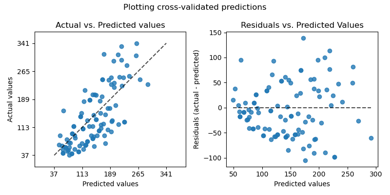
The plot on the left shows the actual values vs predicted values. For a
noise-free regression task aiming to predict the (conditional) expectation of
y, a perfect regression model would display data points on the diagonal
defined by predicted equal to actual values. The further away from this optimal
line, the larger the error of the model. In a more realistic setting with
irreducible noise, that is, when not all the variations of y can be explained
by features in X, then the best model would lead to a cloud of points densely
arranged around the diagonal.
Note that the above only holds when the predicted values is the expected value
of y given X. This is typically the case for regression models that
minimize the mean squared error objective function or more generally the
mean Tweedie deviance for any value of its
“power” parameter.
When plotting the predictions of an estimator that predicts a quantile
of y given X, e.g. QuantileRegressor
or any other model minimizing the pinball loss, a
fraction of the points are either expected to lie above or below the diagonal
depending on the estimated quantile level.
All in all, while intuitive to read, this plot does not really inform us on
what to do to obtain a better model.
The right-hand side plot shows the residuals (i.e. the difference between the
actual and the predicted values) vs. the predicted values.
This plot makes it easier to visualize if the residuals follow and
homoscedastic or heteroschedastic
distribution.
In particular, if the true distribution of y|X is Poisson or Gamma
distributed, it is expected that the variance of the residuals of the optimal
model would grow with the predicted value of E[y|X] (either linearly for
Poisson or quadratically for Gamma).
When fitting a linear least squares regression model (see
LinearRegression and
Ridge), we can use this plot to check
if some of the model assumptions
are met, in particular that the residuals should be uncorrelated, their
expected value should be null and that their variance should be constant
(homoschedasticity).
If this is not the case, and in particular if the residuals plot show some
banana-shaped structure, this is a hint that the model is likely mis-specified
and that non-linear feature engineering or switching to a non-linear regression
model might be useful.
Refer to the example below to see a model evaluation that makes use of this
display.
3.3.5. Clustering metrics
The sklearn.metrics module implements several loss, score, and utility
functions. For more information see the Clustering performance evaluation
section for instance clustering, and Biclustering evaluation for
biclustering.
3.3.6. Dummy estimators
When doing supervised learning, a simple sanity check consists of comparing
one’s estimator against simple rules of thumb. DummyClassifier
implements several such simple strategies for classification:
-
stratifiedgenerates random predictions by respecting the training
set class distribution. -
most_frequentalways predicts the most frequent label in the training set. -
prioralways predicts the class that maximizes the class prior
(likemost_frequent) andpredict_probareturns the class prior. -
uniformgenerates predictions uniformly at random. -
constantalways predicts a constant label that is provided by the user.-
A major motivation of this method is F1-scoring, when the positive class
is in the minority.
Note that with all these strategies, the predict method completely ignores
the input data!
To illustrate DummyClassifier, first let’s create an imbalanced
dataset:
>>> from sklearn.datasets import load_iris
>>> from sklearn.model_selection import train_test_split
>>> X, y = load_iris(return_X_y=True)
>>> y[y != 1] = -1
>>> X_train, X_test, y_train, y_test = train_test_split(X, y, random_state=0)
Next, let’s compare the accuracy of SVC and most_frequent:
>>> from sklearn.dummy import DummyClassifier
>>> from sklearn.svm import SVC
>>> clf = SVC(kernel='linear', C=1).fit(X_train, y_train)
>>> clf.score(X_test, y_test)
0.63...
>>> clf = DummyClassifier(strategy='most_frequent', random_state=0)
>>> clf.fit(X_train, y_train)
DummyClassifier(random_state=0, strategy='most_frequent')
>>> clf.score(X_test, y_test)
0.57...
We see that SVC doesn’t do much better than a dummy classifier. Now, let’s
change the kernel:
>>> clf = SVC(kernel='rbf', C=1).fit(X_train, y_train)
>>> clf.score(X_test, y_test)
0.94...
We see that the accuracy was boosted to almost 100%. A cross validation
strategy is recommended for a better estimate of the accuracy, if it
is not too CPU costly. For more information see the Cross-validation: evaluating estimator performance
section. Moreover if you want to optimize over the parameter space, it is highly
recommended to use an appropriate methodology; see the Tuning the hyper-parameters of an estimator
section for details.
More generally, when the accuracy of a classifier is too close to random, it
probably means that something went wrong: features are not helpful, a
hyperparameter is not correctly tuned, the classifier is suffering from class
imbalance, etc…
DummyRegressor also implements four simple rules of thumb for regression:
-
meanalways predicts the mean of the training targets. -
medianalways predicts the median of the training targets. -
quantilealways predicts a user provided quantile of the training targets. -
constantalways predicts a constant value that is provided by the user.
In all these strategies, the predict method completely ignores
the input data.